Distribution of Benefits in Teacher Retirement Systems and - Eric

Distribution of Benefits in

Teacher Retirement Systems and

Their Implications for Mobility

RobeRt CostRell

and MiChael PodguRsky

w o r k i n g p a p e r 3 9 • d e c e m b e r 2 0 0 9

Distribution of Benefits in Teacher Retirement Systems and Their Implications for Mobility

Robert M. Costrell University of Arkansas

Michael Podgursky

University of Missouri – Columbia

Corresponding authors: Robert M. Costrell ([email protected]), Department of Education Reform, University of Arkansas and Michael Podgursky ([email protected]), Department of Economics, University of Missouri – Columbia.

mailto:[email protected]

mailto:[email protected]

The authors wish to acknowledge support from the National Center on Performance Incentives at Vanderbilt University. They also appreciate the excellent research assistance of Joshua McGee. The authors are also grateful for support from the National Center for Analysis of Longitudinal Data in Education Research (CALDER), supported by Grant R305A060018 to the Urban Institute from the Institute of Education Sciences, U.S. Department of Education.

CALDER working papers have not gone through final formal review and should be cited as working papers. They are intended to encourage discussion and suggestions for revision before final publication.

The Urban Institute is a nonprofit, nonpartisan policy research and educational organization that examines the social, economic, and governance problems facing the nation. The views expressed are those of the authors and should not be attributed to the Urban Institute, its trustees, or any of the funders and organizations. All errors are those of the authors. CALDER, The Urban Institute 2100 M Street N.W., Washington, D.C. 20037 202-261-5739 • www.caldercenter.org

i

http://www.caldercenter.org/

CONTENTS

Abstract iii Introduction 1

How Teacher Pensions Work 4

Pension Wealth and Cumulative Earnings 9

Measuring Redistribution of Benefits in Teacher Retirement Systems 14

Penalties for Mobility 20

Mobility Loss by Age of Move 31

Empirical Relevance 38 Conclusion 39 References 44

ii

Distribution of Benefits in Teacher Retirement Systems and Their Implications for Mobility Robert Costrell and Michael Podgursky CALDER Working Paper No. 39 December 2009

ABSTRACT

While it is generally understood that defined benefit pension systems concentrate benefits on career

teachers and impose costs on mobile teachers, there has been very little analysis of the magnitude of

these effects. The authors develop a measure of implicit redistribution of pension wealth among

teachers at varying ages of separation. Compared to a neutral system, often about half of an entering

cohort’s net pension wealth is redistributed to teachers who separate in their fifties from those who

separate earlier. There is some variation across six state systems. This implies large costs for interstate

mobility. Estimates show teachers who split a thirty-year career between two pension plans often lose

over half their net pension wealth compared to teachers who complete a career in a single system. Plan

options that permit purchases of service years mitigate few or none of these losses. It is difficult to

explain these patterns of costs and benefits on efficiency grounds. More likely explanations include

the relative influence of senior versus junior educators in interest group politics and a coordination

problem between states.

iii

INTRODUCTION Traditional teacher pension plans have long been understood to concentrate benefits on career

teachers and impose costs on mobile teachers. However, there has been little or no attempt to

measure the extent of this redistribution of benefits from short-term to long-term teachers or the

costs of mobility for those who cross state lines. Nor has there been a detailed examination of

the key features of pension plans that account for these phenomena. In this paper we offer the

first measurements of the degree of redistribution and mobility costs imposed by typical pension

systems and an analysis of plan features that generate them.

In recent years, several developments have made these issues timely. The first has been a

heightened focus on teacher quality. This leads directly to questions about whether

compensation systems—including pension policy—are designed to optimally attract and retain

the highest quality teachers at any given cost. Secondly, on the supply side, young educated

workers are highly mobile, and there is evidence that job mobility has grown in recent decades.1

If teacher pension systems lack portability and back-load benefits more so than other sectors, this

may put K-12 employers at a competitive disadvantage in recruiting young college-educated

workers.

In addition to these demand and supply factors, another trend, at work for several

decades, has been the evolution of teacher pension plans themselves. In general, there has been a

tendency to reduce pension plans’ normal retirement age and also to expand or enhance early

retirement provisions. Since life spans have been increasing at the same time, the span of

retirement years widens.

1 See Jaeger and Stevens (1999), Stewart (2002).

1

For this and other reasons, teacher pension plans—like other public pension plans—have

become more costly. Looking at employer contributions alone, figure 1 (updated from Costrell

and Podgursky, 2009b) provides evidence of the growing gap between K-12 and private sector

benefit costs. Here we report BLS quarterly employer retiree benefit costs (including Social

Security) for public school teachers and private sector managers and professionals for the period

since March 2004 (the first quarter in which the data were released). Figure 1 clearly shows that

these costs as a percent of payroll are larger for public schools and that the gap is widening.2 The

gap still does not reflect the increase in amortization payments that will be required to shore up

funding, from the drop in asset values since 2007. As states re-examine their pension plans for

fiscal reasons, it may also be an opportunity to consider their labor market effects.

In earlier work we focused on the peculiar incentives for retirement built into these

systems. Many of these plans feature large spikes in annual pension wealth accrual for teachers in

their fifties that act to keep midcareer teachers in the classroom, pulling them to the spike and

then pushing them into retirement shortly thereafter as pension wealth accrual turns negative

(Costrell and Podgursky, 2007a,b; 2009a). In this paper, we extend this line of research by

focusing on the distribution of these benefits among teachers of varying career lengths and the

closely related mobility penalties for those who work a full career, but who switch pension

systems.

2 Measuring benefits as a percentage of earnings is the usual convention; reasons for that are discussed in Costrell and Podgursky, 2009b, unabridged, pp. 5‐6. The percentages can also be converted to dollars using the dollar value of earnings. The dollar benefit gaps between teaching and private sector professionals, however, depend on whether one considers hourly, weekly, or annual compensation (Costrell and Podgursky, 2009b, unabridged, pp. 10‐12). The appropriate measure—hourly, weekly, or annual—has been much debated, and this is not the place to revisit those arguments.

2

Figure 1. Employer Contributions for Retirement and Social Security: Public School Teachers and Private Professionals and Managers

11.9 11.9 12.2 12.2 12.3 12.412.8 13.0 12.8 12.8

13.2 13.2 13.4 13.413.9

14.5 14.5 14.6 14.6 14.615.1 15.2

10.0 10.1 10.2 10.310.6 10.5 10.7 10.6 10.5 10.4 10.5

10.0 10.1 10.4 10.5 10.5 10.5 10.4 10.3 10.4 10.3

15.3

10.510.2

4

6

8

10

12

14

16

Mar 04

Jun 0

4

Sep 04

Dec 04

Mar 05

Jun 0

5

Sep 05

Dec 05

Mar 06

Jun 0

6

Sep 06

Dec 06

Mar 07

Jun 0

7

Sep 07

Dec 07

Mar 08

Jun 0

8

Sep 08

Dec 08

Mar 09

Jun 0

9

Sep 09

Perc

ent o

f ear

ning

s

Public K-12 teachers Private management and professional

Source: Costrell and Podgursky (2009b), updated.

BLS, National Compensation Survey, Employer Costs for Employee Compensation.

We analyze the distribution of pension wealth by comparing existing defined benefit

teacher pension systems with fiscally equivalent systems that would have distributionally neutral

accrual paths. Compared to such a system, we find that teacher systems often redistribute about

half the net pension wealth of an entering cohort toward those who separate in their mid-fifties,

from those who leave the system earlier.

This trend has immediate implications for the costs that teacher pension systems impose

on mobile teachers. We are not the first to note that these defined benefit systems impose costs

on individuals who separate before normal retirement age or switch systems—a number of policy

reports have called attention to this problem (e.g., Gates, 1996; Ruppert, 2001; Traurig et al.

3

2001). However, we are unaware of any studies of teacher pensions that undertake a careful

analysis of the accrual of pension wealth over a mobile teacher’s career, and how pension plan

features affect that accrual process. While it is widely understood that final average salary

formulas used in calculating pension annuities produce losses for mobile teachers, it is not as

widely understood that service eligibility rules for normal and early retirement compound these

losses.

The effects of complex pension rules are readily measured by their impact on pension

wealth. In this study we examine pension formulas in six state plans and develop measures of the

implicit redistribution of pension wealth in these systems from teachers who separate early to

those who separate later. We then show how this back-loading produces very large losses in

pension wealth for mobile teachers. Compared to a teacher who has worked 30 years in a single

state system, a teacher who has put in the same years but split them between two systems will

often lose well over one-half of her net pension wealth. We also show that rules permitting

service purchases do very little to ameliorate these losses. We find it difficult to justify, on

efficiency grounds, this system of rewards and penalties which generates such unequal benefits.

HOW TEACHER PENSIONS WORK

Public school teachers are almost universally covered by traditional defined benefit (DB) pension

systems. In such a system, the employer has an obligation to provide a regular retirement check

to employees upon their retirement, based on years of service, possibly age, and final average

salary.

4

Typically, a DB teacher pension plan requires that both teachers and employers make a

contribution each year to a pension trust fund. On average, these contributions are smaller for

the majority of teachers who are part of the Social Security system and larger for those who are

not covered (Costrell and Podgursky, 2009b). Contributions must not only cover the currently

accruing liabilities (known as "normal costs"), but also the amortization of previously accrued

unfunded liabilities (the so-called "legacy costs"). The salient characteristic of a traditional DB

system is that for any individual, benefits are not tied to contributions.

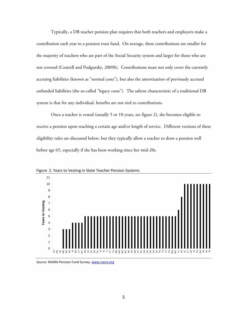
Once a teacher is vested (usually 5 or 10 years, see figure 2), she becomes eligible to

receive a pension upon reaching a certain age and/or length of service. Different versions of these

eligibility rules are discussed below, but they typically allow a teacher to draw a pension well

before age 65, especially if she has been working since her mid-20s.

Figure 2. Years to Vesting in State Teacher Pension Systems

0

1

2

3

4

5

6

7

8

9

10

11

AZ

NH WI

MN

ND

SD IA MS

UT

WY

AR

CA

CO DE

DC HI

ID IL KY LA ME

MD

MO

MT

NE

NV

NM NY

NC

OH

OK

OR PA

SC TN TX VT

VA

WA

WV FL AK AL

CT

GA IN KS

MA MI

NJ RI

Year

s to

Ves

ting

Source: NASRA Pension Fund Survey. www.nasra.org

5

Benefits at retirement are usually determined by a formula of the following sort:

(1) Annual Benefit = m(YOS, Age)·YOS·FAS.

In this expression, YOS denotes years of service, the final average salary (FAS) is an average of the

last few years of salary (typically three) and m is a percentage commonly referred to as the

"multiplier," which may be constant, but is often a function of service and age.3 In Missouri, for

example, teachers at normal retirement earn 2.5 percent for each year of teaching service. Thus,

a teacher with 30 years of service would earn 75 percent of the final average salary. So if the FAS

were $60,000 she would receive:

Annual Benefit = .025 x 30 x $60,000 = $45,000,

payable for life. If the teacher were to separate from service prior to being eligible to receive the

pension, the first draw would be deferred and the amount of the pension would be frozen until

that time. Once the pension draw begins, there is typically some form of inflation adjustment,

although the nature of it varies from state to state.

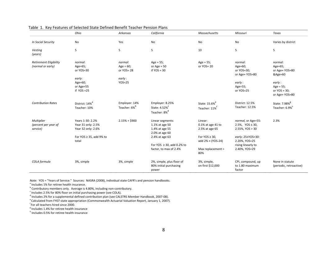
Table 1 summarizes some of the key parameters of DB pension plans in six states. While

not randomly chosen (we inhabit two of these states), they are indicative of many teacher

pension plans.4 More complete versions of such tables are published by the NEA and others,

showing similar variation in these pension parameters across states.5

3 States will often specify a multiplier for "normal" retirement, but also have various "early" retirement provisions that can be expressed as age‐or‐service‐based reductions in the "normal" multiplier.

4 These six states account for 29 percent of total Fall 2004 employment of public school teachers. (U.S. Department of Education, 2007, Table 63). 5 NEA (2004), Loeb and Miller (2006).

6

7

The complexity of the formula varies from state to state. Arkansas, for example, has a

relatively simple formula. Once an educator reaches age 60 or 28 years of service, she can draw a

pension equal to the final average salary times 2.15 percent times years of service (plus $900 per

year).6 She can start drawing the pension earlier, after 25, 26, or 27 years of service, but with an

adjustment of 85, 90, or 95 percent, respectively. The formulas for other states are more

complicated, as we shall see below.

6 This refers to "contributory" members. There has also been a "non‐contributory" option that provides lesser benefits. Our analysis of Arkansas pension wealth, below, also excludes the "T‐DROP" program.

8

Table 1. Key Features of Selected State Defined Benefit Teacher Pension Plans Ohio Arkansas California Massachusetts Missouri Texas

In Social Security

No Yes No No No Varies by district

Vesting (years)

5 5 5 10 5 5

Retirement Eligibility (normal or early)

normal: Age=65; or YOS=30 early: Age=60; or Age=55 if YOS =25

normal: Age = 60; or YOS= 28 early : YOS=25

Age = 55; or Age = 50 if YOS = 30

Age = 55; or YOS= 20

normal: Age=60; or YOS=30; or Age+ YOS=80 early : Age=55; or YOS=25

normal: Age=65; or Age+ YOS=80 &Age=60 early : Age = 55; or YOS = 30; or Age+ YOS=80

Contribution Rates District: 14%

a Teacher: 10%

Employer: 14% Teacher: 6%b

Employer: 8.25% State: 4.52%c

Teacher: 8%d

State: 15.6%e

Teacher: 11%f

District: 12.5% Teacher: 12.5%

State: 7.98%g Teacher: 6.9%h

Multiplier (percent per year of service)

Years 1‐30: 2.2% Year 31 only: 2.5% Year 32 only: 2.6% For YOS ≥ 35, add 9% to total

2.15% + $900 Linear segments: 1.1% at age 50 1.4% at age 55 2.0% at age 60 2.4% at age 63 For YOS ≥ 30, add 0.2% to factor, to max of 2.4%

Linear: 0.1% at age 41 to 2.5% at age 65 For YOS ≥ 30, add 2% × (YOS‐24) Max replacement = 80%

normal, or Age=55: 2.5%, YOS ≤ 30, 2.55%, YOS > 30 early: 25≤YOS<30: 2.20%, YOS=25 rising linearly to 2.40%, YOS=29

2.3%

COLA formula 3%, simple 3%, simple 2%, simple, plus floor of

80% initial purchasing power

3%, simple, on first $12,000

CPI, compound, up to 1.80 maximum factor

None in statute (periodic, retroactive)

Note: YOS = "Years of Service." Sources: NASRA (2008), individual state CAFR’s and pension handbooks. a Includes 1% for retiree health insurance. b Contributory members only. Average is 4.80%, including non‐contributory. c Includes 2.5% for 80% floor on initial purchasing power (see COLA). d Includes 2% for a supplemental defined contribution plan (see CALSTRS Member Handbook, 2007‐08). e Calculated from FY07 state appropriation (Commonwealth Actuarial Valuation Report, January 1, 2007). f For all teachers hired since 2000. g Includes 1.4% for retiree health insurance h Includes 0.5% for retiree health insurance

The composite effect of these systems—whether they are simple or complex—is hard to discern

from the system’s parameters. To appreciate the strong distributional impact of these systems, and thus

make informative comparisons among states, we use these parameters to compute patterns of pension

wealth accumulation by age of separation.7

PENSION WEALTH AND CUMULATIVE EARNINGS

The parameters of teacher pension plans can be used to estimate the value of pension benefits using the

concept of pension wealth. This concept reflects both the size of the annual pension payment and the

number of years for which it is received. When an individual retires under a DB plan he or she is

entitled to a stream of payments that has a lump sum value—the present discounted value—which can

be readily determined using standard actuarial methods.

Formally, consider an individual’s pension wealth, P, at some potential age of separation, As.

The stream of expected payments may begin immediately, or may (perhaps must) be deferred until some

later retirement age. The present value of those payments is:

(2) ( )( ) ( ) ( ),||)( sAA

sAA

s AABAAfi1APs

s ⋅+= ∑≥

−

7 Teacher pension formulas are generally similar in structure to those of state employees. In some states the formulas are identical and in other states the eligibility rules favor earlier retirement for teachers. On the other hand, public safety workers will typically be eligible for earlier retirement than teachers. Among private sector workers, DB pensions are vanishing. Beginning in the 1980s, many private‐sector employers shifted to defined contribution plans. Of those private employers who have maintained DB systems, many have opted for cash balance or hybrid systems. Twenty five percent of private sector workers covered by DB plans are now cash balance DB plans (more on this below). An example of a hybrid plan is the federal civil service, which replaced its traditional DB plan with a hybrid plan combining a thrift (DC) plan, along with a reduced DB pension. See Hansen (2009), Costrell, Johnson, and Podgursky (2009). In the 1980s, when traditional DB plans were more common in the private sector, they were much studied and the accrual patterns were calculated. In examining this literature, we found (Costrell and Podgursky 2009a) that those spikes were dwarfed in size by the teacher pension spikes we have studied, typically by an order of magnitude.

9

where B(A│As) is the defined benefit one will receive at age A, (as specified in equation (1)), given that

one has separated at age As, f(A│As) is the conditional probability of survival to that age, and i is the

discount rate.8

In principle, P(As) represents the market value of the annuity. If, instead of providing a promise

to pay annual benefits, the employer were to provide a lump sum of this magnitude upon separation, the

employee could buy the same annuity on the market. The teacher’s pension wealth, P(As), is the size of

the 401(k) that would be required to generate the same stream of payments she would be owed upon

separation at age As.

Figure 3 depicts pension wealth, in inflation-adjusted dollars, for a 25-year-old entrant to the

Missouri teaching force who works continuously until leaving service at various ages of separation. The

salary schedule assumed is that of the state capital (Jefferson City), under which teachers receive annual

step increases and also lane increases as they move from a bachelor’s degree to a master’s degree. The

entire salary grid is assumed to increase at 2.5 percent inflation. We assume a 5 percent discount rate,9

and use the most current female mortality tables (2004) from the CDC.10 The results are shown for

gross pension wealth, given by P(As), and net pension wealth, subtracting the cumulative value of

employee contributions.

8 The benefit stream may itself be a choice among alternative streams open to the individual, based upon the choice of when to begin receiving payments. Often, the best choice is simply to receive benefits as soon after separation as possible, but not always, since there may be an age reduction in benefits for receipt prior to “normal” retirement age. In modeling pension wealth below, we assume that individuals separating at age As will choose the stream of payments that maximizes present value.

9 There is a dispute between financial economists and actuaries regarding the prudent discount rate. The 5 percent figure here is closer to the economists’ recommendation than that of the actuaries, who typically use about 8 percent. The higher discount rate will affect the dollar amount for Figure 3 (e.g. the gross pension wealth for a teacher separating at age 56 drops from $898,000 to $653,000), but will not have much effect on the shapes of the diagrams. It is the shapes that drive our main results, regarding the percentages of pension wealth redistributed by length of career and lost due to mobility.

10 Most teachers are female. For males, the pension wealth is a bit lower, due to shorter life expectancies, but the curves have very similar shapes.

10

Figure 3. Pension Wealth, Missouri Female Teacher (adjusted for inflation)

$0

$100,000

$200,000

$300,000

$400,000

$500,000

$600,000

$700,000

$800,000

$900,000

$1,000,000

26 27 28 29 30 31 32 33 34 35 36 37 38 39 40 41 42 43 44 45 46 47 48 49 50 51 52 53 54 55 56 57 58 59 60 61 62 63 64 65age at separation (entry age = 25)

Slow growth prior to age 46. pension draw must be deferred to age 60.

Faster growth, from age 46 to 49. “Rule of 80” reduces deferral to age 56.

Jump in pension wealth at age 50.“25-and-out” makes draw immediate: gain 6 years of pension payments.

Phase-down of early retirement penalty.

"Rule of 80" kicks in again.31-year bonus.

net of employee contributions

The accumulation of pension wealth is not smooth and steady, but rises with fits and starts, due to rules

of eligibility for early retirement and the like. To illustrate with the case of Missouri, after vesting at 5

years this teacher’s pension wealth grows steadily to age 45, reaching about $200,000 in gross pension

wealth, representing the present value of a steadily growing annuity collectible at age 60. The curve gets

steeper at age 46, because Missouri’s "rule of 80" would allow such a teacher, leaving with 21 years of

service, to collect her pension for an extra year, starting at age 59. The rule of 80 continues to add an

extra year of pension benefits for each additional year of service up to age 49, at which point she need

only defer her pension to age 56. Then, there is a big jump at age 50, because her 25th year of service

makes her eligible for an immediate pension (albeit with a reduced multiplier). This adds 6 years worth

of pension payments to what she had been eligible for at age 49. Growth continues to be rapid in

subsequent years as the multiplier is increased to its “normal” rate of 2.5 percent. Following a final

11

bump to the multiplier at 31 years of service (age 56), growth in pension wealth slows, and pension

wealth net of employee contributions (shown on the lower curve) actually declines. We have gone

through this detail to illustrate how the complex pension rules, replete with discontinuities, not only

lead to pension wealth curves that are irregularly shaped, but more specifically, bear no resemblance to

the smoothly growing cumulative value of contributions.

Cumulative earnings, with accrued interest, evaluated at the age of separation are:

(3) ( )( ) ( ),)( 1∑<

−−+=s

s

AA

AAs AWi1AE

where W(A) is one’s annual wage at age A. Teacher and employer contributions are typically fixed

percentages of earnings, call them ct and ce, so their cumulative values are simply ct · E(As) and ce · E(As).

Net pension wealth, depicted in Figure 3, is Pnet(As)= P(As) - ct · E(As).

Since pension wealth is the present value of a stream of payments going forward and cumulative

earnings is the present value of a stream of payments going backwards, both evaluated at the same point

in time (at age As), they are comparable measures capitalizing these two components of compensation.

Figure 4 depicts gross and net pension wealth as a percentage of cumulative earnings, P(As)/E(As) and

Pnet(As)/E(As). The two curves differ simply by the teacher’s contribution rate, 12.5 percent in Missouri,

for the year depicted. These measures have a fairly intuitive interpretation. Net pension wealth,

Pnet(As)/E(As), expresses deferred compensation as a percent add-on to compensation during one’s

working life. Thus, an individual separating at age 53 receives gross pension benefits worth 47.8 percent

of cumulative earnings, for a net fringe benefit rate of 35.3 percent. Conversely, an individual

separating at age 30 would receive gross pension benefits worth only 10.3 percent of cumulative

earnings, and negative 2.2 percent net of employee contributions, so this individual (and others up to

12

age 34) would be better off withdrawing her contributions, even though she is vested (that is why, in

figure 3 and other figures, we have bounded net pension wealth at zero).

The pension wealth measure P(As)/E(As) also has a more concrete interpretation from the

funding side. It represents the percentage of earnings that must be set aside each year (from employer

and/or employee) in order to fully fund the pension benefits, for any given age of separation.11 Clearly,

those individuals who retire in their mid-to-late-50s receive significantly more in benefits than has been

contributed to the system on their behalf (employer contribution is also 12.5 percent), while those who

separate from service earlier in their career do not. Figure 4 therefore illustrates the uneven distribution

of benefits that is built into the system. In proportionate terms, the net benefits are even more

unequally distributed than the gross benefits. We now turn to our measure of the distribution of

pension wealth, to get a sense of the magnitude of the phenomenon, and also to help us compare states.

Figure 4. Pension Wealth as Percent of Cumulative Earnings, Missouri Female

-10%

0%

10%

20%

30%

40%

50%

26 28 30 32 34 36 38 40 42 44 46 48 50 52 54 56 58 60 62 64

Age at separation (entry age = 25)

Perc

ent o

f cum

ulat

ive

earn

ings

Gross pension wealth Net of employee contributions

11 This does not include contributions required to amortize unfunded liabilities from previous cohorts.

13

MEASURING REDISTRIBUTION OF BENEFITS IN TEACHER RETIREMENT SYSTEMS

We consider the distribution of net pension wealth. As we have seen, teachers separating in their fifties

receive greater net pension wealth than those separating earlier, as a percentage of cumulative earnings.

To develop a measure of redistribution, we consider a benchmark case where net pension wealth is

proportional to cumulative earnings, for comparison with the traditional DB systems. A cash balance

(CB) system provides such a benchmark. CB systems calculate employee retirement accounts, based on

contributions of employees and employers, with a guaranteed rate of return (usually comparable to the

risk-free discount rate recommended by finance economists). Thus, pension wealth—both gross and

net of employee contributions—is a fixed percentage of cumulative earnings, independent of age of

separation. The curves in figure 4 are flat lines under these simple CB systems.

In dollar terms, net pension wealth grows smoothly under such a system, rather than in fits and

starts, as under many DB plans that exhibit kinks in accrual from age and service eligibility rules. Figure

5 compares the accrual of net pension wealth under Missouri’s DB plan (the S-shaped curve, reproduced

from figure 3) with the smooth accrual under a hypothetical CB plan. This diagram readily illustrates

the redistribution of net pension wealth toward those who separate in their fifties from those who

separate earlier (and from the very few who separate later, as well). We now turn to a quantitative

measurement of this redistribution.

14

Figure 5. Net Pension Wealth, Missouri: Actual DB and Hypothetical Cash Balance (adjusted for inflation)

$0

$100,000

$200,000

$300,000

$400,000

$500,000

$600,000

$700,000

$800,000

26 27 28 29 30 31 32 33 34 35 36 37 38 39 40 41 42 43 44 45 46 47 48 49 50 51 52 53 54 55 56 57 58 59 60 61 62 63 64 65Age at separation (entry age = 25)

Actual DB

Cash balance

First we need to define the fiscally equivalent CB plan. To do so, we need to calculate the cost

of the DB plan for the cohort of 25-year-old entrants. This requires weights for age of separation.

These were estimated from longitudinal teacher-level Missouri data. Using data for the 2002 teaching

workforce, we estimated a smooth polynomial function predicting permanent (i.e., at least three

consecutive years) exits as a function of age and experience.12 We found that separations of 25-year-old

entrants are concentrated in the first years of employment, and then in one’s fifties.

In addition to using these weights, we must also adjust for the differences in present value of

pension wealth evaluated at different ages of separation. Formally, we set ce*, the employer contribution

rate for the fiscally equivalent CB plan to satisfy:

12 We fitted a logit function to individual teacher data with sixth order polynomial terms in age and experience and interactions of age and experience up to quadratic. The fitted values were used as weights in these simulations. Similar results were found with Arkansas data.

15

, ( ) ( ) ( ) ( ) ( ) ( ) ( ) ( ) ( )2565

25

2565

25

* 11)4( −−

=

−−

=

+⋅=+⋅⋅ ∑∑ S

s

S

s

AS

net

A

AS

A

e iAPAgiAEAgc SS

where Pnet(As) and E(As) were defined earlier and g(As) is the proportion of the cohort that separates at

any given age (i.e. the weights discussed above). The right-hand side is the present value, as of entry age

25, of the average cohort member’s net pension wealth under the DB plan, and the left-hand side is the

same concept under the CB plan. Each side is also the present value of the employer’s required

contributions under each plan. (Note that this is a “static” fiscal equivalence, since we do not factor in

any behavioral response in the separation weights to the very different incentives of the two plans.)

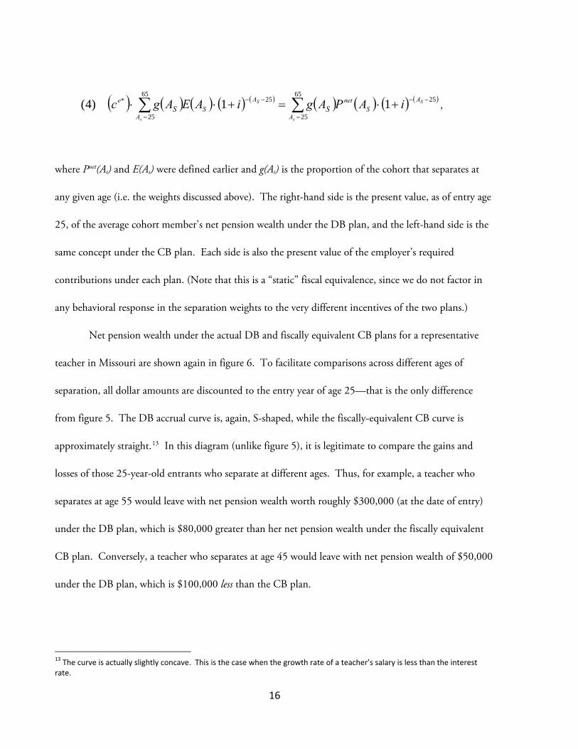
Net pension wealth under the actual DB and fiscally equivalent CB plans for a representative

teacher in Missouri are shown again in figure 6. To facilitate comparisons across different ages of

separation, all dollar amounts are discounted to the entry year of age 25—that is the only difference

from figure 5. The DB accrual curve is, again, S-shaped, while the fiscally-equivalent CB curve is

approximately straight.13 In this diagram (unlike figure 5), it is legitimate to compare the gains and

losses of those 25-year-old entrants who separate at different ages. Thus, for example, a teacher who

separates at age 55 would leave with net pension wealth worth roughly $300,000 (at the date of entry)

under the DB plan, which is $80,000 greater than her net pension wealth under the fiscally equivalent

CB plan. Conversely, a teacher who separates at age 45 would leave with net pension wealth of $50,000

under the DB plan, which is $100,000 less than the CB plan.

13 The curve is actually slightly concave. This is the case when the growth rate of a teacher’s salary is less than the interest rate.

16

We have developed numerical summary statistics for this analysis. Specifically, we calculate the

weighted average of net pension wealth for 25-year-old entrants in Missouri to be $114,283, evaluated

at entry, representing 24 percent of the weighted average of present value of lifetime earnings.14

Compared to the fiscally equivalent CB plan, an average of $52,360 is redistributed—46 percent of

average pension wealth. This represents the average distance between the actual and CB curves in Figure

6. The losers (comprising 65 percent of the cohort, separating at an average age of 36.6) are transferring

an average of $40,299 each to the winners (35 percent of the cohort, separating at an average age of

54.2), who gain an average of $74,726, again evaluated as of entry at age 25.15

Figure 6. PV at Entry of Future Net Pension Wealth, Missouri. 46 Percent of Net Pension Wealth Is Redistributed

$0

$50,000

$100,000

$150,000

$200,000

$250,000

$300,000

$350,000

$400,000


Average gain: $75K

Average loss: $40KCB

DB

14 Note that this far exceeds the 12.5 percent employer contribution rate in Missouri. The reason is that employer contribution rates are calculated to cover liabilities discounted at 8 percent; our discount rate is 5 percent. 15 The average gain or loss, in absolute value, is (0.65 × $40,299) + (0.35 × $74,726) = $52,360, our measure of the average redistribution. This is 46 percent of average net pension wealth, $114,283.

17

We have made the same calculations of the distributional impact of the DB plans in other states.

Table 2 presents summary statistics that provide some basis for rough comparisons. To provide a

common yardstick, each state’s summary statistics are calculated using the same set of separation

weights—the estimated weights from Missouri—even though of course different state pension systems

give somewhat different incentives to separate at various ages. It is possible that comparisons among

states would be affected by using a different state’s set of separation weights. 16 So, for this and other

reasons, the comparisons should not be over-interpreted, especially if states are close in any given

measure.

Table 2. Redistribution of Net Pension Wealth, Compared to Fiscally Equivalent Cash Balance Plan 25‐Year‐Old Entrants a.

Average Net

Pension Wealth Average Redistribution

of Net Gainers Losers

State Dollars

Percent lifetime earnings

Dollars

Percent pension wealth

Share of entrants

Average age at

separation Average gain

Share of entrants

Average age at

separation Average loss

Missouri $114,283 24% $52,360 46% 0.35 54.2 $74,726 0.65 36.6 $40,299

Arkansas $110,911 22% $43,138 39% 0.34 53.9 $62,787 0.66 37.1 $32,856

Ohio $112,400 18% $54,660 49% 0.33 56.4 $83,755 0.67 37.8 $40,567

California $93,401 15% $33,461 36% 0.29 57.8 $56,946 0.71 35.4 $23,690

Texas (new hires) $51,934 10% $24,336 47% 0.35 57.3 $34,601 0.65 34.8 $18,768

Massachusetts $51,812 7% $31,372 61% 0.20 57.1 $80,171 0.80 40.2 $19,502 a All dollar amounts are PV at entry.

That said, some comparisons might be made. The first pair of columns in table 2 provides

estimates of the relative generosity of employer-funded retirement benefits for 25-year-old entrants, both

in dollar terms, and as a percent of lifetime earnings. Missouri, Arkansas, Ohio, and California, with

16It may be argued that by using Missouri weights for other states one underestimates the degree to which teachers in those other states concentrate at the pension spikes, and, therefore, the degree of redistribution. If so, then Missouri’s ranking in degree of distribution may be biased upward.

18

average net pension wealth of approximately $100,000 at entry, are about twice as generous as Texas17

and Massachusetts in dollar terms. As a percent of lifetime earnings, Missouri and Arkansas lead this set

of states, at 22 to 24 percent, while the higher wage states (hence larger denominators) of Ohio and

California follow at 15 to 18 percent. Texas follows at 10 percent (for new hires) and Massachusetts—

the highest wage state, with the lowest average net pension wealth—is the least generous, at 7 percent of

lifetime earnings.

The variations in relative generosity primarily reflect differences in pension wealth for those who

separate in their fifties. They are driven by a few key features of the pension formulas in these states,

including the replacement rate and the eligibility rules for first pension draw. The annuity earned at age

55 is 65-75 percent of final average salary for the top three states in table 2 (Missouri, Arkansas, and

Ohio), as compared to 48-57 percent for the other three states (California, Massachusetts and Texas).

For all six states, a teacher separating at age 55 is eligible for immediate pension (and it is optimal not to

defer), but for those separating a bit earlier, there is important variation in the age of eligibility or

optimality for first draw. For example, upon separating at age 50, the optimal first draw is immediate in

Missouri and Arkansas, which helps explain their relative generosity; for the other states, it is optimal to

defer for three-to-seven years, to ages 53 (Massachusetts), 55 (Ohio and Texas), or 57 (California).18

Our main focus is not the relative generosity, but the degree and nature of each state’s

redistribution of net pension wealth. Column 3 of table 2 provides the average dollar amount of

redistribution. Column 4 represents this as a percent of average net pension wealth (column 1). In all

states, the degree of redistribution is substantial: 36-61 percent of net pension wealth. In Massachusetts,

17 Texas, it should be noted, reduced benefits in 2007—unlike most other states during this period—although this applies only to new hires. For teachers hired before 2006, the average net pension wealth for 25‐year‐old entrants is $73,215 or 14 percent of cumulative earnings, considerably higher than the figures for new hires, $51,934 or 10 percent of cumulative earnings. 18 Employer contributions also vary across these states, so the net pension wealth comparisons are not fully determined by the value and timing of the annuity, but clearly the eligibility rules and replacement rates explain a good portion of the variation in generosity.

19

for example, average pension wealth is low, but most of it is redistributed.19 In all states, the average age

of separation for winners is in the fifties, although there is some variation—the winners are younger in

Missouri and Arkansas than in other states. The average age for losers is usually in the late thirties.20

The redistributive gains are concentrated, while the losses are more dispersed, as indicated in

columns 5 and 8. This is particularly true for Massachusetts, where the gains are concentrated among

one-fifth of the cohort. The average gain in pension wealth for the winners (evaluated at age of entry)

ranges from $34,601 in Texas to over $80,000 in Massachusetts and Ohio. In all states, the losses are

more dispersed, so the average loss is lower, ranging from about $20,000 in California, Texas, and

Massachusetts to about $40,000 in Missouri and Ohio.21

Altogether, there is significant variation among states in the average net pension wealth provided

by their DB systems, and also in the magnitude of the gains and losses relative to a distributionally

neutral CB system. However, all states redistribute net pension wealth to a substantial degree, to those

who separate in their fifties (after about thirty years of service), from those who separate earlier. In

addition to the issue of equity this raises serious issues for educator mobility to which we now turn.

PENALTIES FOR MOBILITY It is widely recognized that DB pensions penalize mobility; however, the sources of these costs are rarely

delineated or quantified in a systematic way. There are several factors that produce pension wealth loss

19 The degree of redistribution increased when Massachusetts enhanced the pension formula in 2001; under the prior formula, the average redistribution was $18,068, or 42 percent of average net pension wealth. 20 The weights for calculating the average ages of winners and losers are the total dollar gains and losses by age of separation. Thus, for example, although 26‐year‐old separators are the most numerous group, their losses are negligible, so they do not weigh heavily in the average age of losers.

21 We are assuming that early separators withdraw their contributions only if that maximizes net pension wealth. It is likely that some (perhaps many) liquidity‐constrained teachers withdraw their contributions even if the net present value of a deferred pension is positive. If that is the case then the redistribution rate from early separators to later separators is larger than we have computed.

20

when a teacher moves. The simplest and most transparent has been termed “non-vested loss.” Teachers

who move before they are vested have no claim on a pension, something new teachers easily understand

(“if I work five years I get a pension; if I quit before then I don’t”). Upon departure, or shortly

thereafter, any teacher contributions are returned with interest (the rate varies, and can be well below

market), but the teacher does not receive employer contributions.22 In general, this is a significant

source of loss for many young teachers, since most teacher pension systems have a vesting period of five

years or longer (figure 2) and the vast majority of early career teacher turnover occurs in the first five

years on the job. That said, our simulations below will assume that teachers move after vesting, so the

mobility loss from not vesting in the first job will not be considered any further.

Even for teachers who are vested there remain potentially large costs from mobility and these are

less transparent. One cost comes from the fact that teacher DB pensions are all final-average-salary

based. When a teacher separates before normal retirement age, the value of her annuity is tied to her

salary at the time of her separation. No adjustment is made for ensuing real salary growth or inflation.

This cost has been termed “deferred pension loss,” but is more accurately referred to as "frozen FAS

loss."23

These costs are routinely identified in policy briefs and reports on DB pension systems and seem

to be understood within the policy community. However, these same reports imply that this is the only,

or at least the predominant, source of loss of pension wealth for mobile vested teachers.24 In fact, there

are other costs to mobility arising from the service eligibility rules for normal and early retirement.

Teachers who separate from a plan with, say, fewer than 20 years of service will often not be able to

22 South Dakota is an interesting and notable exception. See also the next note. 23 South Dakota is an exception on this point as well. That state inflates final salary at 3.1 percent annually up to the normal retirement age. Although the Social Security system indexes earnings to the date of retirement, we are not aware of any state system besides South Dakota that does so. 24 For example, see Ruppert (2001), a reported sponsored by the National Governors Association, the State Higher Education Executive Officers, and the National Conference of State Legislatures.

21

begin collecting their pension until much later than teachers who remain in the plan until meeting

eligibility requirements. This means that at any given age, pension wealth is lower for the mobile

teacher—who has left one system early and entered another system late—simply because she can expect

to collect fewer pension checks. Alternatively, she may be able to draw her pension at the same time as

the teacher who stays in one system, but with a penalty on the multiplier. Either way, as shown below,

the costs associated with these eligibility factors are substantial, and can account for a significant part of

the erosion of pension wealth for a mobile teacher.

Pension wealth calculations such as those in the previous section provide a comprehensive

method for evaluating the costs of mobility. The measures of redistribution illustrate the costs incurred

by a teacher who separates at an early age versus a later age, in the same system. However, in this section

we want to consider the loss in pension wealth for a teacher who changes pension systems. Since we will

be comparing the pension wealth between movers and stayers who retire at the same age—unlike the

previous section’s comparisons—we can revert to calculating wealth as of the date of final separation,

rather than entry.

Specifically, let us continue to assume that a teacher enters at age 25 and works continuously.

However, now rather than assuming that she works continuously in the same system, we assume that at

age 40, after 15 years in state X, she moves to state Y and ultimately separates at age As. (We shall

consider other scenarios below). In this section, we assume she collects two pensions, one in state X and

one in state Y.

Let us also assume that upon re-employment with 15 years experience, she is placed on step 16

of an identical salary grid in her new district, just as if she had been on that grid from entry. In practice,

she probably would not be placed that high, and this would constitute another loss from mobility, not

only in salary, but also in pension (based on final salary), but we leave this aside.

22

Formally, let Pnet(A;Ae,x) denote net pension wealth for a teacher entering in state x at age Ae and

separating at age A. Then the net pension wealth for our mobile teacher, serving 15 years in state X and

ultimately leaving state Y at age As>40 is Pnet(40;25,X)+ Pnet(As;40,Y), where both pieces are evaluated as

of age As. Her loss is:

(6) loss from leaving state X = Pnet(As;25,X) - [Pnet(40;25,X) + Pnet(As;40,Y)]

={[ Pnet(As;25,X) - [Pnet(40;25,X) + Pnet(As;40,X)]}

+{ Pnet(As;40,X) - Pnet(As;40,Y)}.

The second term in braces represents the difference in pension generosity between the two systems, for

teachers spending the latter part of their career in state Y versus state X.25 This can be positive or

negative due to differences in pension formulas. The first term in braces is the pure mobility cost for

state X, and that is what we focus on.

The pure mobility cost for state X can be thought of as the loss from leaving state X and then re-

entering an identical state, with the same pension formula and same pay grid, but with zero creditable

service. It is important to note that in a CB system of the type described earlier, the mobility cost is

zero. That is because the present value of lifetime earnings is the same under either career path (again

assuming no loss in steps upon moving). Therefore, the CB wealth—a fixed percentage of lifetime

earnings—is also unaffected by mobility. But as we have seen in the previous section, the DB wealth

trajectory differs markedly from that of the fiscally equivalent CB plan, redistributing from early

separators to stayers. This inequality is closely related to the cost of mobility.

The hypothetical net wealth trajectory described above—leaving state X and re-entering with

zero service—is illustrated in figure 7 for Missouri. The solid curves depict net pension wealth under

25 A similar calculation for the loss from entering state X from state Y, compared to a full career in state X results in the same expression, except the generosity differential is based on the first years of her career.

23

the DB and fiscally equivalent CB plans, evaluated at date of separation—reproducing figure 5. The

dotted curves represent the wealth trajectories for those who move after 15 years, at age 40. For the CB

plan, the mover’s wealth trajectory lies on top of the stayer’s—there is no loss from mobility.

For the DB plan, however, the paths diverge in year 16 at age 41 and thereafter. The dotted

line is the sum of net pension wealth from the two pensions. For the first five years, the dotted line is

flat since the teacher is not yet vested in the new system. The difference here between the solid and

dotted lines is the vesting loss discussed above, in the second job. However, the loss does not vanish, but

continues to widen in the years immediately following vesting. The stayer’s wealth trajectory accelerates

at certain points, due to the "rule of 80" and "25-and-out" provisions, which advance the first pension

draw. The mover, however, enjoys no such acceleration—her accrual is relatively smooth—because she

never meets the eligibility requirements for retiring before age 60.

Figure 7. Net Pension Wealth, Missouri: Movers vs. Stayers, DB and CB. 65 Percent Loss from Mobility for Age 55 Separator: $407K

$0

$100,000

$200,000

$300,000

$400,000

$500,000

$600,000

$700,000

$800,000


stay move

CB

DB

One pension, at 55

Both pensions deferred to 60

24

Specifically, under a continuous career, she would obtain 30 years of service by age 55 qualifying

her for “normal” retirement benefits immediately at 75 percent of final average salary. This is worth

$626,088 (inflation-adjusted) at age 55. Under the broken career, the teacher receives two annuities,

each of which is for 37.5 percent of final average salary, but the FAS for the first pension is of course

much lower. This is the “frozen FAS loss” described above. In addition, neither the first nor the second

pension would be drawn until “normal” retirement at age 60; “early” retirement options are available,

but the penalties in this case favor deferral. This means that five years of pension payments are lost

(along with the inflation adjustments for those years). These two factors together reduce the net pension

wealth to $219,163, a loss from mobility of $406,925, evaluated at age 55. This is the gap between the

dotted and solid curves in figure 7 at age 55. The cost of mobility is 65 percent of net pension wealth.26

Note that for later separation ages, the mobility loss from delayed first draw diminishes, since

the stayer is forgoing pension payments herself. If she stays to age 60, there is no difference in the

timing of pension checks between her and her mobile alter ego. For final separation beyond age 60, the

mobile teacher actually has an advantage on the first pension, since that can still be collected at age 60.

This contributes to the narrowing of the gap between the dotted and solid DB curves.27 Figures 8-12

similarly depict the costs of mobility for our five other states.

26 For gross pension wealth, the loss is identical in dollars, but lower in percent—47 percent in this case.

27 Indeed, in the case of Massachusetts, those who separate at age 65 fare less well as stayers than as movers, as shown in Figure 12. For movers, the first pension would be optimally collected starting at age 55, a full ten years earlier than for stayers, which outweighs the fact that the first pension’s FAS is smaller. There is another advantage to splitting up the pension in MA, due to the nature of the COLA.

25

Figure 8. Net Pension Wealth, Arkansas: Movers vs. Stayers. 54 Percent Loss from Mobility for Age 55 Separator: $312K

$0

$100,000

$200,000

$300,000

$400,000

$500,000

$600,000

$700,000

$800,000

26 27 28 29 30 31 32 33 34 35 36 37 38 39 40 41 42 43 44 45 46 47 48 49 50 51 52 53 54 55 56 57 58 59 60 61 62 63 64 65


stay move

One pension, at 55


Figure 9. Net Pension Wealth, Ohio: Movers vs. Stayers. 74 Percent Loss from Mobility for Age 55 Separator: $522K

$0

$100,000

$200,000

$300,000

$400,000

$500,000

$600,000

$700,000

$800,000

$900,000

$1,000,000

26 27 28 29 30 31 32 33 34 35 36 37 38 39 40 41 42 43 44 45 46 47 48 49 50 51 52 53 54 55 56 57 58 59 60 61 62 63 64 65


stay move

One pension, at 55


26

Figure 10. Net Pension Wealth, California: Movers vs. Stayers. 41 Percent Loss from Mobility for age 55 Separator: $201K

$0

$100,000

$200,000

$300,000

$400,000

$500,000

$600,000

$700,000

$800,000

$900,000

$1,000,000

26 27 28 29 30 31 32 33 34 35 36 37 38 39 40 41 42 43 44 45 46 47 48 49 50 51 52 53 54 55 56 57 58 59 60 61 62 63 64 65

Age at separation (entry age = 25)stay move

One pension, at 55


Figure 11. Net Pension Wealth, Texas (New Hires): Movers vs. Stayers. 73 Percent Loss from Mobility for Age 55 Separator: $197K

$0

$100,000

$200,000

$300,000

$400,000

$500,000

$600,000

$700,000

$800,000

26 27 28 29 30 31 32 33 34 35 36 37 38 39 40 41 42 43 44 45 46 47 48 49 50 51 52 53 54 55 56 57 58 59 60 61 62 63 64 65


stay move

One pension, at 55


27

Figure 12. Net Pension Wealth, Massachusetts: Movers vs. Stayers. 58 Percent Loss from Mobility for Age 55 Separator: $195K

$0

$100,000

$200,000

$300,000

$400,000

$500,000

$600,000

$700,000

$800,000


stay move

One pension, at 55

Both pensions draw at 55

(but lose 30-yr bump)

28

Table 3 provides summary calculations of these mobility losses for all six states. Again, these are

pension wealth losses for a 25 year-old entrant who spends her first 15 years on another (but similar)

teaching job. Consider the entries for Missouri. The first two columns give the dollar loss from

mobility for a 55-year-old separator, evaluated at age 55 (as depicted in figure 7), and as evaluated at

entry (for comparison with the previous section). Either way, the mover suffers a loss of 65 percent of

her pension wealth as compared to the stayer. A glance down the third column shows substantial

mobility costs in all six states, ranging from 41 percent to 74 percent. The next three columns indicate

the age of first pension draw for 55-year-old separators; for stayers, it is immediate, but for movers, it is

deferred on both pensions, except for Massachusetts.

Table 3. Losses from Mobility. 25‐Year‐Old Entrants, 15 Years in First Job

Age 55 separators: Average separator over 50: loss from mobility vs. DB loss from mobility vs. DB stayers

State

Dollar loss of pension wealth, evaluated at 55

Dollar loss of pension wealth, evaluated at entry

Loss as percent

of stayers' pension wealth

First draw: stayers

First draw: movers, 1st

pension

First draw: movers, 2nd

pension

Dollar loss of pension wealth,

evaluated at entry

Loss as percent of stayers' pension wealth

Missouri $406,925 $197,493 65% 55 60 60 $180,731 62%

Arkansas $312,335 $151,586 54% 55 60 60 $138,074 51%

Ohio $522,865 $253,762 74% 55 60 60 $194,933 67%

California $201,409 $97,750 41% 55 57 57 $80,779 36%

Texas (new hires) $197,220 $95,717 73% 55 63 63 $85,002 65%

Massachusetts $194,627 $94,458 58% 55 55 55 $62,416 47%

The last two columns compute the weighted average loss over all teachers who separate after the

age of 50 (as opposed to just those at 55).28 Again, the losses for the mobile teacher are substantial,

28 Again, the weights are those of Missouri. Note also that the dollar losses cannot be calculated at exit, since we are averaging over different exit years. So they are evaluated at the common entry age.

29

ranging from 36 percent to 67 percent. Overall, the average loss from mobility is roughly half the net

pension wealth of stayers.

Finally, consider figure 13, which decomposes the mobility loss in each of the six states, for 55-

year-old separators who split their career. For each state, the full bar depicts the net pension wealth for a

teacher who stays in a single state system. The bottom bar, in dark gray, depicts the net pension wealth

for the teacher who moves. The other bars, representing the difference between the two, depict the

losses from mobility, decomposed by source.

Figure 13. Decomposition of Loss from Mobility. Entry at 25, Move at 40, Retire at 55a

$(200,000)

$(100,000)

$-

$100,000

$200,000

$300,000

$400,000

$500,000

$600,000

$700,000

$800,000

Missouri Arkansas Ohio California Texas MassachusettsNet

Pen

sion

Wea

lth a

t Age

55

(infla

tion-

adju

sted

)

mobile teacher loss from frozen FAS loss from reduced % FAS loss from delayed 1st draw

Deferral raises pension

Early retirement

penalty

Lose 30-yr bump

60vs.55

60vs.55

60vs.55

63vs.55

57 vs.55

a Losses from each source taken separately over‐explain the mobility loss. In this chart, the interaction term is allocated

proportionately among the three sources

30

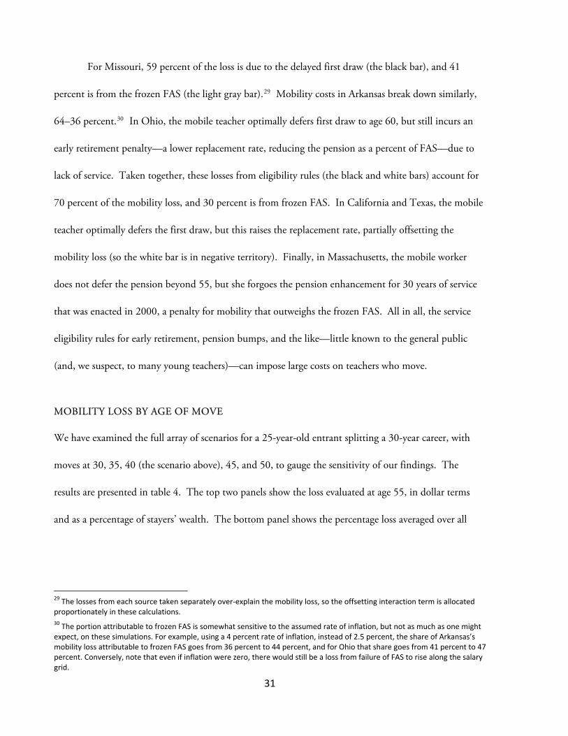
For Missouri, 59 percent of the loss is due to the delayed first draw (the black bar), and 41

percent is from the frozen FAS (the light gray bar).29 Mobility costs in Arkansas break down similarly,

64–36 percent.30 In Ohio, the mobile teacher optimally defers first draw to age 60, but still incurs an

early retirement penalty—a lower replacement rate, reducing the pension as a percent of FAS—due to

lack of service. Taken together, these losses from eligibility rules (the black and white bars) account for

70 percent of the mobility loss, and 30 percent is from frozen FAS. In California and Texas, the mobile

teacher optimally defers the first draw, but this raises the replacement rate, partially offsetting the

mobility loss (so the white bar is in negative territory). Finally, in Massachusetts, the mobile worker

does not defer the pension beyond 55, but she forgoes the pension enhancement for 30 years of service

that was enacted in 2000, a penalty for mobility that outweighs the frozen FAS. All in all, the service

eligibility rules for early retirement, pension bumps, and the like—little known to the general public

(and, we suspect, to many young teachers)—can impose large costs on teachers who move.

MOBILITY LOSS BY AGE OF MOVE

We have examined the full array of scenarios for a 25-year-old entrant splitting a 30-year career, with

moves at 30, 35, 40 (the scenario above), 45, and 50, to gauge the sensitivity of our findings. The

results are presented in table 4. The top two panels show the loss evaluated at age 55, in dollar terms

and as a percentage of stayers’ wealth. The bottom panel shows the percentage loss averaged over all

29 The losses from each source taken separately over‐explain the mobility loss, so the offsetting interaction term is allocated proportionately in these calculations. 30 The portion attributable to frozen FAS is somewhat sensitive to the assumed rate of inflation, but not as much as one might expect, on these simulations. For example, using a 4 percent rate of inflation, instead of 2.5 percent, the share of Arkansas’s mobility loss attributable to frozen FAS goes from 36 percent to 44 percent, and for Ohio that share goes from 41 percent to 47 percent. Conversely, note that even if inflation were zero, there would still be a loss from failure of FAS to rise along the salary grid.

31

separations beyond age 50. Each panel clearly shows that for all states except Texas, the pension loss is

almost as large for moving at ages 35 or 45, as it is for the move at 40.31

Table 4. Losses from Mobility, by Age of Move. 25‐Year‐Old Entrants

Dollar loss of pension wealth, evaluated at 55 MO AR OH CA TX MA Move at age 30 $103,629 $171,436 $325,119 $142,902 $41,191 $165,359 Move at age 35 $382,152 $302,756 $511,689 $199,585 $101,863 $181,455 Move at age 40 $406,925 $312,335 $522,865 $201,409 $197,220 $194,627 Move at age 45 $403,286 $295,605 $518,967 $194,691 $144,596 $187,742 Move at age 50 $29,943 ($1,375) $374,435 $139,454 $82,701 $229,885

Percent loss of pension wealth, evaluated at 55 MO AR OH CA TX MA Move at age 30 17% 29% 46% 29% 15% 49% Move at age 35 61% 52% 72% 41% 38% 54% Move at age 40 65% 54% 74% 41% 73% 58% Move at age 45 64% 51% 73% 40% 54% 56% Move at age 50 5% 0% 53% 28% 31% 68%

Percent loss of pension wealth, average 50+ MO AR OH CA TX MA Move at age 30 31% 36% 44% 23% 16% 34% Move at age 35 55% 49% 65% 35% 40% 42% Move at age 40 62% 51% 67% 36% 65% 47% Move at age 45 62% 48% 66% 34% 51% 56% Move at age 50 1% ‐3% 44% 25% 30% 56%

31 For Texas, having 20 years of service in either the first or second job (accrued by moving at 45 or 35, respectively), allows one to draw the pension at 60 without penalty under the "rule of 80." This is notably better than one can do with only 15 years in each job (accrued by moving at 40), so the loss from mobility is notably lower by moving at 35 or 45 in Texas.

32

Figure 14 illustrates the case of Missouri. The top curve is the stayer’s pension wealth and the

four other curves represent wealth accrual for those who move at ages 30, 35, 40, and 45. The latter

three curves indicate no appreciable difference in pension wealth at 55 for those who move at ages 35–

45.

Figure 14. Net Pension Wealth, Missouri: Movers vs. Stayers, by Age of Move

$0

$100,000

$200,000

$300,000

$400,000

$500,000

$600,000

$700,000

$800,000


stay move at 30 move at 35 move at 40 move at 45

The pension loss is typically much smaller if one moves early, at age 30, since 25 years in the

second job will often suffice to secure an immediate pension at age 55, eliminating much of the loss.32

Conversely, late career moves, at age 50, can also reduce the pension loss, for the same reason, as 25

years on the first job will often allow one to draw the first pension at age 55 or even at 50. Indeed, in

some states, if one is willing to work a few years beyond 55 on the second job, one can do significantly

32 Massachusetts is the main exception among our six states. That is because the main loss from moving at 40 is the failure to secure the 30‐year bump, and that is still true for those who move at age 30.

33

better than staying a full career in one system. As figure 15 shows, for Missouri, such a move can allow

pension wealth to continue accruing after accrual turns negative for the stayer.

Figure 15. Net Pension Wealth, Missouri: Move at 50 vs. Stay

$0

$100,000

$200,000

$300,000

$400,000

$500,000

$600,000

$700,000

$800,000

$900,000


stay move

1st pension at 50, 2nd at 60

One pension, at 55

In theory, the large mobility costs we have calculated could be ameliorated if agreements could be

reached for reciprocity regarding service years between the systems. While there have been discussions

of developing such reciprocity agreements, to date, we are aware of no two states where this exists.33

Given the variation between states in benefit formulas and teacher contribution rates, undoubtedly there

is concern about ensuring even exchanges of net benefits. There is no guarantee that the flows between

two states would be balanced—teachers might start their careers in Maine and end them in Florida. The

fact that teachers in some states are covered by Social Security while others are not further complicates

33 In some states, reciprocity agreements do exist among systems managed by the state, e.g., between state employees and teacher pensions in Missouri. However, they do not exist between teacher pension funds across state lines. Even in regions with considerable teacher and administrator mobility, such as New England, there has been no development of interstate reciprocity in educator retirement systems.

34

matters. In addition to these difficulties, commentators have noted that teacher pension boards tend to

be dominated by long term employees or pension recipients, so the problems of short term, mobile

teachers have traditionally received less attention (Gates, 1996).34

Given the failure to develop interstate reciprocity agreements, it is sometimes claimed that the

mobility problem is partly ameliorated by rules permitting the purchase of service credits by mobile

teachers (Gates, 1996; Ruppert, 2001). When a vested teacher terminates membership in a pension

system, she has the option of withdrawing her contributions. For example, in Texas, teachers who

withdraw from the system can take their contributions plus five percent annual interest. Most states

allow experienced teachers who transfer in to purchase service years for prior experience, up to a limit –

usually the minimum of prior service years or years in the current system. Thus, a teacher with ten years

of teaching experience in a Missouri public school who moves to Texas can purchase a year of experience

for every year of Texas service, up to a maximum of ten years. Arkansas, Florida and Ohio will permit

no more than five years of purchases regardless of the number of years of prior out-of-state experience.

The rules for these purchases can be complicated. Most systems charge prices that reflect the

actuarial cost of service years, either averaged over all teachers or customized for the teacher in question.

Examples of the former are Arkansas, Missouri, and Florida, which charge the teacher the same rate as

the combined employer and employee contributions for the year in which she makes the purchase. This

rate, of course, reflects the normal actuarial costs plus amortization of unfunded liabilities for the entire

system (not just the teacher in question). Other states, such as Texas and California, charge the mobile

teacher an actuarial rate based upon the age of the teacher making the purchase. In this case, the rate is

lower for young teachers and rises with age.

34 Interest in the topic seems to have peaked with the previous bull market in equities (Ruppert, 2001; Traurig, 2001). We could find little discussion of such reforms since.

35

In either case the funds she has available from cashing out of her old system typically fall far

short of what is necessary to purchase the same number of years in the new system or maintain

equivalent pension wealth. The reason for this shortfall is that a teacher typically receives on cashing out

of her pension plan her contributions only, with some rate of annual interest. Teacher contributions are

usually no more than one half of total contributions, as indicated in table 1. Teachers in states with low

teacher contribution rates, in general, are not going to be able to repurchase most of their service years

when they change systems. This point is illustrated in table 5 below for a hypothetical teacher moving

from California to teach in another state.

We assume our representative teacher enters at age 25 and teaches continuously. In this case we

assume that she has taught for 15 years in the Sacramento school district and is thus vested in the

California teacher retirement system. When she moves she has the option of leaving the California system

and withdrawing her contributions along with compound interest of 5.25 percent. Netting out inflation,

fifteen years of her contributions would give her a real balance of $44,296. Assuming that she moved on

to a teaching job that paid what she would have earned had she stayed in Sacramento (again, net of

inflation), how many years of teaching service could she buy in these systems? In no case can she come

close to purchasing 15 years. At best, she can manage between 2.8 and 3.8 years in the new system.

Table 5. Maximum Service Years a Mobile California Teacher Can Purchase by Withdrawing Her Pension System Contributions a

40‐year‐old teacher, 15 years experience in CA, employed at step 16 in State: Years purchased Missouri 2.8 Texas 3.8 Arkansas 3.4 Florida 3.7

36

a A California teacher employed in the Sacramento school district, who contributes 6 percent annually to the state teacher retirement fund, takes a job in the indicated state earning the inflation‐adjusted salary she would have earned at step 16 on the Sacramento schedule. She withdraws her contributions (plus 5.25 percent interest) and purchases the maximum number of service years those funds permit in the new pension system.

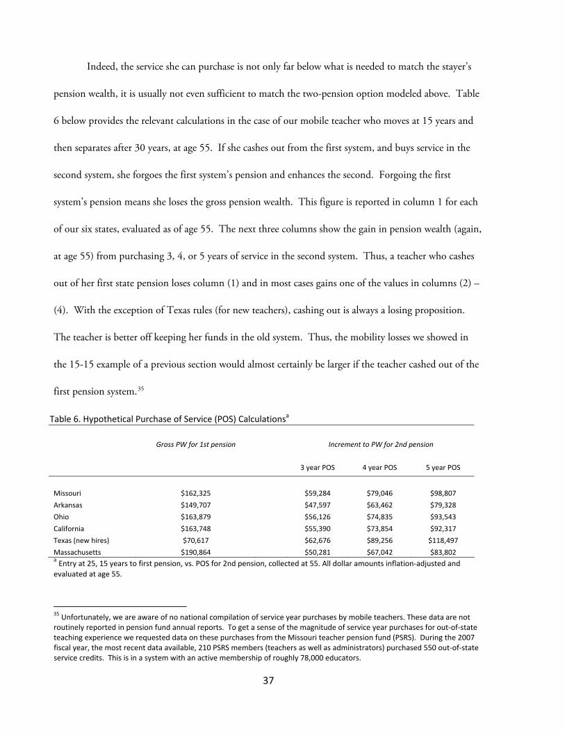
Indeed, the service she can purchase is not only far below what is needed to match the stayer’s

pension wealth, it is usually not even sufficient to match the two-pension option modeled above. Table

6 below provides the relevant calculations in the case of our mobile teacher who moves at 15 years and

then separates after 30 years, at age 55. If she cashes out from the first system, and buys service in the

second system, she forgoes the first system’s pension and enhances the second. Forgoing the first

system’s pension means she loses the gross pension wealth. This figure is reported in column 1 for each

of our six states, evaluated as of age 55. The next three columns show the gain in pension wealth (again,

at age 55) from purchasing 3, 4, or 5 years of service in the second system. Thus, a teacher who cashes

out of her first state pension loses column (1) and in most cases gains one of the values in columns (2) –

(4). With the exception of Texas rules (for new teachers), cashing out is always a losing proposition.

The teacher is better off keeping her funds in the old system. Thus, the mobility losses we showed in

the 15-15 example of a previous section would almost certainly be larger if the teacher cashed out of the

first pension system.35

Table 6. Hypothetical Purchase of Service (POS) Calculationsa Gross PW for 1st pension Increment to PW for 2nd pension

3 year POS 4 year POS 5 year POS

Missouri $162,325 $59,284 $79,046 $98,807

Arkansas $149,707 $47,597 $63,462 $79,328

Ohio $163,879 $56,126 $74,835 $93,543

California $163,748 $55,390 $73,854 $92,317

Texas (new hires) $70,617 $62,676 $89,256 $118,497

Massachusetts $190,864 $50,281 $67,042 $83,802 a Entry at 25, 15 years to first pension, vs. POS for 2nd pension, collected at 55. All dollar amounts inflation‐adjusted and evaluated at age 55.

35 Unfortunately, we are aware of no national compilation of service year purchases by mobile teachers. These data are not routinely reported in pension fund annual reports. To get a sense of the magnitude of service year purchases for out‐of‐state teaching experience we requested data on these purchases from the Missouri teacher pension fund (PSRS). During the 2007 fiscal year, the most recent data available, 210 PSRS members (teachers as well as administrators) purchased 550 out‐of‐state service credits. This is in a system with an active membership of roughly 78,000 educators.

37

EMPIRICAL RELEVANCE What is the empirical relevance of these findings? Specifically, if educator labor markets are local—with

low rates of interstate mobility—does it really matter how large these penalties are? Our examination of

the evidence indicates that interstate mobility is sufficiently important that the penalties for interstate

mobility do matter in practice.36

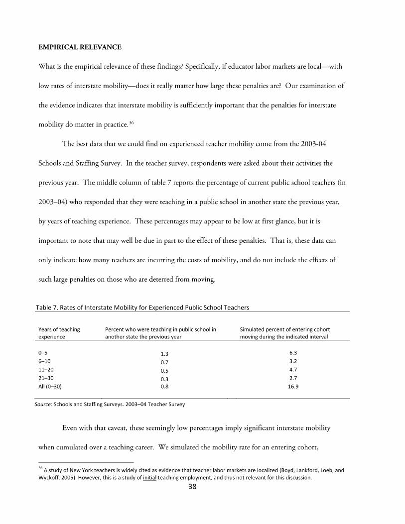
The best data that we could find on experienced teacher mobility come from the 2003-04

Schools and Staffing Survey. In the teacher survey, respondents were asked about their activities the

previous year. The middle column of table 7 reports the percentage of current public school teachers (in

2003–04) who responded that they were teaching in a public school in another state the previous year,

by years of teaching experience. These percentages may appear to be low at first glance, but it is

important to note that may well be due in part to the effect of these penalties. That is, these data can

only indicate how many teachers are incurring the costs of mobility, and do not include the effects of

such large penalties on those who are deterred from moving.

Table 7. Rates of Interstate Mobility for Experienced Public School Teachers

Years of teaching experience

Percent who were teaching in public school in another state the previous year

Simulated percent of entering cohort moving during the indicated interval

0–5 1.3 6.3 6–10 0.7 3.2 11–20 0.5 4.7 21–30 0.3 2.7 All (0–30) 0.8 16.9

Source: Schools and Staffing Surveys. 2003–04 Teacher Survey

Even with that caveat, these seemingly low percentages imply significant interstate mobility

when cumulated over a teaching career. We simulated the mobility rate for an entering cohort,

36 A study of New York teachers is widely cited as evidence that teacher labor markets are localized (Boyd, Lankford, Loeb, and Wyckoff, 2005). However, this is a study of initial teaching employment, and thus not relevant for this discussion.

38

assuming no one moves more than once. The results, reported in the last column of table 7, suggest that

about one-sixth of teachers move across state lines sometime during a 30-year career. Of these, about

one-third would move prior to completing one’s fifth year of service and the median move would be at

8–9 years. It is perhaps not surprising that so many of the moves would be early-career, given both the

intrinsic propensity to move when young, reinforced by the strong penalties for moving later. It is,

however, noteworthy that as many as one-third of the movers do so between 10 and 20 years, despite

being the years of maximum penalty. Thus, a significant number of teachers do incur large mobility

losses, and there are likely more that are deterred from moving by these penalties.

CONCLUSION

This paper contributes to the teacher quality and compensation literature by analyzing the distribution

of net pension benefits among teachers of varying ages of separation and the corresponding costs that

teacher pension systems impose on mobile teachers. We are not the first to note that these defined

benefit systems impose costs on individuals who separate before normal retirement age or switch

systems. However, we are unaware of any studies of teacher pensions that estimate the patterns of such

costs—and the reasons for them—through analysis of the accrual of pension wealth at varying ages of

separation, and the pension plan rules which govern that process.

We examined pension wealth accrual in six state plans and developed measures of the unequal

distribution of benefits. Compared to a distributionally neutral system, we find that typically about half

an entering cohort’s net pension wealth is redistributed to teachers who separate in their fifties, from

those who separate earlier. One of the main reasons for this is that teachers who remain into their fifties

can start collecting their pension immediately, while teachers who separate earlier often must defer their

pension (e.g. to age 60), so they collect fewer payments over their retirement.

39

We showed how this inequality in benefits produces very large losses in pension wealth for

mobile teachers. We estimate that teachers who split a thirty-year career between two pension plans

often lose over half their net pension wealth compared to teachers who complete a career in a single

system. This result is robust with regard to whether the move is made at 10, 15, or 20 years, and in

some states the loss is also large even for moves as early as 5 years. Again, one of the main reasons for

this loss is that teachers who split their career often cannot begin collecting pension payments as early as

those who stay in one system. We also show that rules permitting service purchases do very little to

ameliorate the loss from mobility.

Our discussion has focused on teachers. However, the problems we have identified generalize to

other professional staff in public schools. To the extent that markets extend beyond state borders for

any K–12 professionals, the problem arises. School administrators are always included in teacher

retirement systems and increasingly their market is becoming regional or national in scope. For

example, even modest-sized school districts routinely advertise vacancies for principals and

superintendents regionally or nationally, and hire national consulting firms to conduct these searches. A

visit to the national web sites of professional associations, or perusal of their national publications, finds

many advertisements for vacancies. Yet for mobile administrators, retirement benefit systems with five

to ten year vesting can have a devastating effect on retirement benefits, a fact which has not escaped the

notice of some school administrators (Chion-Kenney 1999; Wilson 2001).37

The impediments to mobility—both for teachers and administrators—may be particularly

problematic for charter schools. Currently, just over one million students are enrolled in charter

schools. Many of these schools are part of organizations (e.g., KIPP Academies, Edison, Imagine 37 Ironically, these features of pension systems can actually raise the already high level of retirement benefit costs. In the current school year in Missouri, the combined contribution rate for retirement benefits is 27 percent, with no salary cap, yet examination of Missouri superintendent contracts finds many that provide additional funds, over and above these mandatory contributions, to purchase retirement annuities for mobile (or potentially mobile) superintendents.

40

Schools) operating in more than one state. Edison Learning, for example, operates schools in 16 states.

As these schools attempt to replicate their school models it is valuable to them to move staff from one

location to another, particularly when starting up new schools, in much the same way business firms

relocate managers. As we have shown, these educator retirement benefit systems make this relocation

very costly.

We find it difficult to justify such a system of rewards and penalties on efficiency grounds.38 To

take yet one final example, consider the large differences in the growth of public school enrollment

between states. Figure 16 reports NCES projections of the growth of public K–12 enrollment between

2005 and 2017 in the fastest and slowest growing states. On the one hand states such as Nevada and

Arizona are forecasted to have enrollment growth in excess of 40 percent over this period. At the same

time, Louisiana, Vermont and Rhode Island can expect declines of ten percent or more. Heavily

populated states such as Michigan and New York can expect declines of between five and six percent. In

a well functioning labor market, one would expect to see mobility of teachers from declining towards

expanding teacher labor markets. Instead, the pension system tends to lock public school teachers into

labor markets in which their skills are in declining demand, by imposing large costs on those who move.

38 There is an economics literature analyzing pensions as efficient market responses (e.g., Lazear, 1986). However, the key features in these models that make pensions efficient labor market contracts—efficiency wages or firm‐specific human capital – seem irrelevant in the K‐12 context. The first type of model, efficiency wages, argues that the prospect of a pension keeps workers from shirking, for fear of dismissal. However, by the time public school teachers are vested in their pension systems they are tenured in their jobs. Dismissal for shirking is simply not an option for most employers. Second, pension models grounded in firm‐specific human capital investments are irrelevant since, in the case of teacher pensions, the “firm” is the entire state. Teachers are free to take their pension benefits, and their human capital, to thousands of schools within the state pension plan. It might be argued that teacher pension systems, by impeding interstate mobility, prevent the efficiency loss of state‐specific human capital, but it seems unlikely that such state‐specificity is very strong.

41

Figure 16. Projections of Public School K‐12 Enrollment: 2005 to 2017

44.843.2

32.9

28.927.5 27.1

23.1

‐12.2 ‐11.7 ‐11.4

‐8.0 ‐7.6‐6.3 ‐6.2 ‐5.2

‐4.0

‐20.0

‐10.0

0.0

10.0

20.0

30.0

40.0

50.0

AZ NV TX FL UT GA NC LA VT RI ME ND CT MI NY MA

Percen

t change

Source: U.S. Department of Education. National Center for Education Statistics.

http://www.nces.ed.gov/programs/projections/projections2017/sec1c.asp

The barriers to reform most likely lie in classical political economy. First, states have a

coordination problem. It is in no state’s individual interest to facilitate mobility out of the state; each

state would like to keep its labor supply large and retain the products of its teacher education programs.

Thus, states are inclined to keep average pension costs low by skimping on benefits for those who

depart. Furthermore, even if states wanted to facilitate mobility, it is difficult to break out of a back-

loaded system. If an individual leaves state X with 15 years of service and a pension worth $100,000,

the state could, in principle, transfer the $100,000 to the teacher’s new state Y for 15 years of credit in

that state. However, those years of credit would typically raise the value of the pension in state Y by far

more than $100,000, due to service-based eligibility rules for early retirement. So state Y would not

42

http://www.nces.ed.gov/programs/projections/projections2017/sec1c.asp

accept $100,000 as the price for granting 15 years of service credit, and state X would not offer more

than $100,000.39

In addition to coordination problems between states, the distribution of benefits within states

between short- and long-termers will be governed by the relative influence of junior versus senior

educators in educator groups and state politics. Influence generally increases with seniority for a variety

of reasons, and these are enhanced in the case of pension politics, because the benefits of pensions are far

more immediate and tangible for senior educators than junior ones. This is especially true, given the

opaque nature of final-average-salary DB systems, with complicated eligibility rules.

These barriers are not insurmountable. Similar issues arise in higher education, and yet the

benefits of academic mobility have led many state and private universities to offer more portable

retirement plans.40 As states grapple with the pension difficulties they now face, they should take the

opportunity to consider systems with smooth wealth accrual such as the CB plan modeled in this paper.

Another alternative to consider might be a hybrid, such as TIAA-CREF, which has features of both CB

and defined contribution that have proven so popular in higher education. Such systems are more

transparent, tie benefits more closely to contributions, and do not penalize mobility or job-shopping

among young teachers. More generally, education policy-makers should consider experiments that

provide actuarially fair alternatives to traditional DB plans for new teaching recruits, and evaluate their

utility in the recruitment and retention of high-quality teachers.

39 We note once again that this market failure would not occur if states X and Y had smooth accrual of pension wealth as in the cash balance benchmark we have used. In this case, the additional pension wealth provided to the teacher in her new state (Y) would simply be the $100,000 paid by state X. She would suffer no loss and neither would state Y.

40 This in fact seems to have been an important element in South Dakota’s unusually portable pension system for K‐12. South Dakota, a small state, merged its various pension systems some years ago, and to maintain satisfaction among its higher education members, portability features were extended to all.

43

REFERENCES

Arkansas Teacher Retirement System. 2007. Policies, Rules, and Regulations. Little Rock, AR. http://artrs.gov/index.php?option=com_content&task=view&id=127&Itemid=1

———. 2008. Comprehensive Annual Financial Report, 2007. Little Rock, AR.

http://artrs.gov/Forms/ATRS_10008_07_Annual_Report%202.pdf Boyd, Donald J., Hamilton Lankford, Susanna Loeb, and James H.Wyckoff. 2005. “The Draw of

Home: How Teachers’ Preferences for Proximity Disadvantage Urban Schools.” Journal of Policy Analysis and Management 24(1): 113–32.

California State Teachers’ Retirement System. 2007. Member Handbook, 2007–08. West Sacramento,

CA. http://www.calstrs.com/Help/forms_publications/printed/2007MBRHB/MH_Entire.pdf ———. 2008. Comprehensive Annual Financial Report, 2007. West Sacramento, CA.

http://www.calstrs.com/Help/forms_publications/printed/CurrentCAFR/CAFRall.pdf Chion-Kenney. 1999. “The Perils of Pension Portability.” The School Administrator. Costrell, Robert M., and Michael J. Podgursky. 2007a. “Efficiency and Equity in the Time Pattern of

Teacher Pension Benefits: An Analysis of Four State Systems.” Working Paper 6. Washington, DC: The National Center for Analysis of Longitudinal Data in Education Research, The Urban Institute. http://www.caldercenter.org/PDF/1001070_Efficiency_Equity.pdf

———. 2007b. “Golden Peaks and Perilous Cliffs: Rethinking Ohio’s Teacher Pension System,”

Washington, D.C.: Thomas B. Fordham Institute. http://edexcellence.net/doc/060707_Pensions_Report.pdf

———. 2009a. “Peaks, Cliffs and Valleys: The Peculiar Incentives in Teacher Retirement Systems and

their Consequences for School Staffing.” Education Finance and Policy 4(2): 175–211. ———. 2009b. “Teacher Retirement Benefits: Are Employer Contributions to Teachers’ Retirement

Higher than for Private-Sector Professionals?” Education Next 9(2): 58–63. http://media.hoover.org/documents/ednext_20092_58_unabridged.pdf.

Costrell, Robert M., Robert W. Johnson, and Michael J. Podgursky. 2009. “Modernizing Teacher Retirement Benefit Systems.” In Creating a New Teaching Profession, edited by Dan Goldhaber and Jane Hannaway. Washington, DC: Urban Institute Press.

Gates, Gary I. 1996. Pension Portability for State and Local Government. New York: Milbank Memorial

Fund. Hansen, Janet. 2009. “An Introduction to Teacher Retirement Benefit Systems.” Nashville, TN:

National Center on Performance Incentives, Peabody College, Vanderbilt University.

44

http://artrs.gov/index.php?option=com_content&task=view&id=127&Itemid=1

http://artrs.gov/Forms/ATRS_10008_07_Annual_Report%202.pdf

http://www.calstrs.com/Help/forms_publications/printed/2007MBRHB/MH_Entire.pdf

http://www.calstrs.com/Help/forms_publications/printed/CurrentCAFR/CAFRall.pdf

http://www.caldercenter.org/PDF/1001070_Efficiency_Equity.pdf

http://edexcellence.net/doc/060707_Pensions_Report.pdf

http://media.hoover.org/documents/ednext_20092_58_unabridged.pdf

Jaeger, David A., and Ann Huff Stevens. 1999. “Is Job Stability in the United States Falling? Reconciling Trends in the Current Population Survey and Panel Study of Income Dynamics.” Journal of Labor Economics 17(4) pt. 2, Changes in Job Stability and Job Security: S1-S28.

Lazear, Edward. 1986. “Retirement from the Labor Force.” In Handbook of Labor Economics, vol. 1,

edited by O. Ashenfelter and R. Layard (305–55). New York: Elsevier Science. Loeb, Susanna, and Luke C. Miller. 2006. “State Teacher Policies: What Are They, What Are Their

Effects, and What Are Their Implications for School Finance?” Stanford University: Institute for Research on Education Policy and Practice.

Massachusetts State Teachers’ Retirement System. 2006. Your MTRS Benefits: A Guide for Active

Members. Cambridge, MA. http://www.mass.gov/mtrs/7pubs/77pdfs/actguids.pdf. National Association of State Retirement Administrators. 2008. Public Fund Survey. Baton Rouge, LA.

http://www.publicfundsurvey.org/www/publicfundsurvey/actuarialfundinglevels.asp. National Education Association. 2004. Characteristics of Large Public Education Pension Plans.

Washington, DC. Public Employee Retirement Administration Commission, Commonwealth of Massachusetts. 2007.

Commonwealth Actuarial Valuation Report, 2007. Boston, MA. http://www.mass.gov/perac/valuation/2007commonwealth.pdf.

Public School and Education Employee Retirement Systems of Missouri. 2007. Comprehensive Annual

Financial Report, 2007. Jefferson City, MO. http://www.psrs-peers.org/Investments/2007%20Annual%20Report/2007%20CAFR%20Financial%20Section.pdf.

Public School Retirement System of Missouri. 2007. Member Handbook, 2007-08. Jefferson City, MO.

http://www.psrs-peers.org/PSRS/2007-2008PSRSHandbook/Service%20Retirement.pdf. Ruppert, Sandra S. 2001. Improving Pension Portability: A Report of the SHEEO Project “Enhancing the

Teaching Profession: The Importance of Mobility to Recruitment and Retention. Denver, CO: State Higher Education Executive Officers.

State Teachers Retirement System of Ohio. 2007a. Comprehensive Annual Financial Report, 2007. http://www.strsoh.org/pdfs/CAFR2007/2007_CAFR.pdf.

———. 2007b. Service Retirement and Plans of Payment. http://www.strsoh.org/pdfs/brochures/15-

126.pdf. Stewart, Jay. 2002. “Recent Trends in Job Stability and Job Security: Evidence from the March CPS.”

Working Paper 356. Washington, DC: Bureau of Labor Statistics, U.S. Department of Labor.

45

http://www.mass.gov/mtrs/7pubs/77pdfs/actguids.pdf

http://www.publicfundsurvey.org/www/publicfundsurvey/actuarialfundinglevels.asp

http://www.mass.gov/perac/valuation/2007commonwealth.pdf

http://www.psrs-peers.org/Investments/2007%20Annual%20Report/2007%20CAFR%20Financial%20Section.pdf



http://www.psrs-peers.org/PSRS/2007-2008PSRSHandbook/Service%20Retirement.pdf

http://www.strsoh.org/pdfs/CAFR2007/2007_CAFR.pdf

http://www.strsoh.org/pdfs/brochures/15-126.pdf

http://www.strsoh.org/pdfs/brochures/15-126.pdf

Teacher Retirement System of Texas. 2007a. Comprehensive Annual Financial Report, 2007. Austin, Texas. http://www.trs.state.tx.us/about/documents/CAFR.pdf#CAFR.

———. 2007b. TRS Benefits Handbook. Austin, Texas.

http://www.trs.state.tx.us/benefits/documents/benefits_handbook.pdf. Traurig, Greenberg LLP. 2001. “Removing Pension Barriers to Teacher Mobility in the Mid-Atlantic

Region.” Temple University: Mid-Atlantic Regional Teachers Project. U.S. Department of Education. 2007. “Digest of Education Statistics 2007.” Washington, DC.

http://www.nces.ed.gov/programs/digest/d07/tables/dt07_063.asp. Wilson, Laval. 2001. “My Perils with Pension Portability.” The School Administrator.

46

http://www.trs.state.tx.us/about/documents/CAFR.pdf#CAFR

http://www.trs.state.tx.us/benefits/documents/benefits_handbook.pdf

http://www.nces.ed.gov/programs/digest/d07/tables/dt07_063.asp

Distribution of Benefits in Teacher Retirement Systems and - Eric

Documents

Transcript of Distribution of Benefits in Teacher Retirement Systems and - Eric