Distribution Network Design: Selection and Sizing of

Congested Connections

Simin Huang, Rajan Batta and Rakesh Nagi

Department of Industrial Engineering, 342 Bell Hall,University at Buffalo (SUNY), Buffalo, NY 14260, USA

Revised: November 2004April 2004

Abstract

This paper focuses on certain types of distribution networks in which commodity flows must

go through connections that are subject to congestion. Connections serve as transshipment

and/or switching points and are modeled asM/G/1 queues. The goal is to select connections,

assign flows to the connections, and size their capacities, simultaneously. The capacities are

controlled by both the mean and the variability of service time at each connection. We

formulate this problem as a mixed integer nonlinear optimization problem for both the fixed

and variable service rate cases. For the fixed service rate case, we prove that the objective

function is convex and then develop an outer approximation algorithm. For the variable

service rate case, both mean and second moment of service time are decision variables. We

establish that the utilization rates at the homogeneous connections are identical for an op-

timal solution. Based on this key finding, we develop a Lagrangian relaxation algorithm.

Numerical experiments are conducted to verify the quality of the solution techniques pro-

posed. The essential contribution of this work is the explicit modeling of connection capacity

(through the mean and the variability of service time) using a queueing framework.

Keywords: Distribution network; Connections; Congestion.

1 Introduction

Certain types of distribution networks require that flows between origin-destination node

pairs pass through connections. These connections serve as transshipment and/or switching

points. The application we had in mind for a connection is a distribution center (DC) –

goods flow into the DC from manufacturing plants and are later shipped to fulfill customer

demand. Several multinational companies use distribution center networks in this manner.

For example, a paper products company needs to distribute paper towels, toilet tissue,

napkins, etc. These products are light but are bulky. They cannot be compressed for

transportation or storage purposes as they will lose their shape. Transportation and storage

cost for such items is very high in comparison to the cost of the items themselves, and their

large storage volume causes congestion in the DC. In such an industry setting, selection and

sizing of distribution centers is a problem of much significance. We further note that our

focus is not on industries where there is relatively less congestion and large economies of

scale are realized by traveling through connections; for example, the hub-and-spoke network

in an airline industry.

For most fast moving consumer goods, demand patterns are quite erratic, being a function

of both sales promotions (i.e., seasonal) and regular demand. In response to this, at the

strategic or aggregate level, the production schedules for individual SKUs (Stock Keeping

Units) in a shared facility can be characterized as random variates. We can therefore model

the flows to a DC as a Poisson process. Items are stored at a DC for an arbitrary period of

time and are later retrieved when a customer demand needs to be fulfilled. The residence

time in a DC is a function of the extent of supply chain coordination and the degree of

1

automation in information and material flow. Much of this is in the control of management,

albeit at a cost. We assume a general distribution for the residence time variable. Effectively,

we model a DC as an M/G/1 queueing system and control its capacity through both the

mean and the variability of service time at each connection. By a judicious choice of flows of

items to DCs we can control these storage delays and also influence transportation cost. We

therefore consider the problem of selecting the connections to open, assigning flows to them,

and sizing their capacities simultaneously, in order to minimize overall system cost, i.e., the

sum of transportation cost, service cost (service time plus waiting time), and connection

installation cost (could be a function of its capacity).

We provide a simple numerical example to demonstrate the importance of modeling

congestion for this problem. Suppose there are four flows with amount 5 units each and

two connection candidates with a fixed charge cost of 10. The flow travel times by way of

connections are as follows:

⎛⎜⎜⎜⎝

F low1 F low2 F low3 F low4

Connection1 1 1 1 1

Connection2 2 2 2 2

⎞⎟⎟⎟⎠

We compare three alternatives in the example: (i) using a fixed charge facility location

model without modeling of congestion; (ii) modeling congestion with a fixed rate; and (iii)

modeling congestion with variable rate. Total cost is the sum of transportation cost, service

cost (service time plus waiting time), and connection installation cost (see details later). In

case (i) and (ii), each connection is an M/G/1 queueing system with fixed mean service time

and its second moment. Suppose that the mean service time is 0.048 and its second moment

is 0.02. According to the models we present later, we have optimal solutions for these cases

2

as follows:

• No modeling of congestion: all flows will go to connection 1 with utilization rate 0.96

and total cost 201.79.

• Fixed rate: 13 units of flow will go to connection 1 with utilization rate 0.62 and 7

units go to connection 2 with utilization rate 0.34. The total cost is 194.86.

• Variable rate: all flows will go to connection 1 with utilization rate 0.60 and total cost

108.65. Its mean service time is 0.03 and the second moment 0.045.

This simple example illustrates that modeling congestion with variable capacity size (or rate)

in such distribution networks can lead to significant saving for the system.

Most earlier work in joint sizing and location are in a deterministic setting (e.g. Huang,

Batta, and Nagi (2003)). The originality of the present paper is the explicit modeling of

connection capacity (controlled by the mean and the variability of service time) using a

queueing framework. The consideration of service time variability is an important issue in

the design of a queueing facility. The influence of the variability is illustrated by Hillier

and So (1991), Melnyk, Denzler, and Fredendall (1992), and Enns (1998). However, this

explicit consideration of capacity introduces numerous technical challenge, since the objective

function and the constraints become highly non-linear. The traditional approaches to deal

with the difficulties are to simplify models by either assuming constant variance or constant

coefficient of variation. The methodology we adopt to address these technical difficulties is

unique. We first establish an equal utilization property for the connections and then use this

property to drive the solution methodology. Without this approach the problem remains

highly intractable.

3

Two cases of the problem are considered in this paper. For the fixed service rate case,

we assume that the capacity of each connection is unchangeable. In the variable service

rate case we assume that the capacity of connections is to be determined. The resulting

mathematical formulations are mixed integer nonlinear programs (MINLP). For the fixed

service rate case, we establish a convexity property and develop an outer approximation

algorithm. For the variable service rate case, we show that the optimal utilization rate

at each selected connection should be equal when the cost of unit capacity is independent

of connection location. This key finding enables us to find bounds for total number of

connections and total service rate. Also, an efficient Lagrangian relaxation algorithm is

developed based on these results.

The rest of this paper is organized as follows: Section 2 reviews related research on this

problem. Section 3 provides some preliminaries. Section 4 analyzes the fixed service rate

case, proves the convexity property of this problem, and develops an outer approximation

algorithm for this case. Section 5 details the variable service rate case. We establish that

the utilization rates at the connections are identical for an optimal solution along with

other properties about how to determine this. Based on this key property, we develop a

Lagrangian relaxation algorithm. Section 6 presents computational performance for both

algorithms. Finally, Section 7 provides a summary and suggests directions for future work.

2 Review of Related Literature

These are several other loosely related models that have been developed in the OR/MS

literature that help view our model in a broader context.

4

The hub-and-spoke network model presented in O’Kelly (1986) involves locating a set

of fully interconnected facilities called hubs, which serve as transshipment points for flows

between specified origin and destination nodes. The major assumption in this model is that

the travel cost for inter-hub movement is less than the cost for movement between a hub

and a spoke (due to economies of scale). Campbell (1994) presents an integer programming

formulation for the capacitated hub location problem, in which he takes the hub installation

cost into consideration and restricts the sum of the flows entering any hub to be less than

the capacity of that hub. Other capacitated hub location problems can be found in Aykin

(1994) and Ebery et al. (2000). The difference between the hub-and-spoke network model

and ours is that while we do not consider economies of scale for travel cost we do consider

the queueing behavior of connections.

Another related work is the flow-capturing (or discretionary service facility) model in-

troduced independently by Berman, Larson, and Fouska (1992) and Hodgon (1990). It is

motivated by applications such as locating gas stations. The problem is formulated on a

transportation network with customers traveling on pre-planned paths. It assumes that a

customer will use a facility only if it lies on the pre-planned path. The objective is to maxi-

mize the utilization by customers. The difference between this problem and ours is that the

flow-capturing model tries to attract more customers while our models try to spread flows

in order to reduce congestion.

There are some other location models that take congestion into consideration. The

stochastic queue median (SQM) model due to Berman and Larson (1982) considers locating

a mobile server to minimize the average response time. Berman, Larson, and Parkan (1987)

develop two heuristics for locating p facilities on a congested network. Batta, Ghose, and

5

Palekar (1989) solve this problem for the Manhattan metric with arbitrary shaped barriers

and convex forbidden regions. In the SQM problem, the arrival rate at each facility is

known and the service rate is a function of facility location. In our case, the arrival rate

at each connection is not fixed and the service rates are possible decision variables. Recent

facility location problems with congestion can be found in Marianov (2003), who formulates

a model to locate multiple-server congestible facilities in order to maximize total expected

demand; and Wang, Batta, and Rump (2002), who study a facility location problem with

stochastic customer demand and immobile servers to minimize customers’ total traveling

cost and waiting cost. Again, the sizing of facilities are not considered in these models.

Capacity planning is considered in the design of flexible manufacturing systems. Queueing

networks are applied to control the service rate, the number of servers, input rates, etc. There

are many pieces of work that use queueing network models e.g., see papers by Yamazaki,

Sakasegawa, and Shanthikumar (1992), Yao and Kim (1987), Shanthikumar and Yao (1988),

Bitran and Tirupati (1989) and Bretthauer (1995). For a comprehensive review of queueing

system design problem the reader is referred to Crabill, Gross, and Magazine (1977) and

Stidham (2002). These models only consider what happens at the facilities and are suitable

for the design problems where the travel distances between facilities can be ignored.

Brimberg, Mehrez, and Wesolowsky (1997) and Brimberg and Mehrez (1997) consider

the allocation of a set of servers across queueing facilities so as to best service demand. This

is another way to define the capacity or size of a facility and is hence related to our work.

However, we note that our model also considers location of facilities in addition to sizing

and flow assignment.

6

3 Preliminaries

We assume that connections will be selected from a set of candidate sitesK and let |K| = nK ,

where | · | denotes a set’s cardinality. Let N be set of origins and destinations; their locations

are assumed to be given, with |N | = nN . Each pair of origin and destination is connected

through a connection facility. A is the set of origin-destination pairs. The term fij represents

the flow amount from origin node i to destination node j, for (i, j) ∈ A. We assume that

fij > 0 for all (i, j) ∈ A. This will simplify our presentation of the formulation, proofs

and analysis. If some fij are equal to zero we can reformulate the problem by only defining

decision variables for i, j combinations that have fij > 0. The terms dik and dkj represent the

shortest distances from node i to connection k and from connection k to node j, respectively;

v is the travel speed of the flows; Fk is the fixed installation cost that is related to connection

k. We let α be the net present value (see, e.g., Park (2002)) of per unit time per unit flow

evaluated over the system’s lifetime.

Let λk, S̄k, and S̄2k be the total flow, mean service time, and the second moment of service

time at connection k, respectively. Let xijk be the fraction of flow i-j by way of connection

k; and yk = 1 if a connection is located at candidate site k, and 0 otherwise.

We use the notation ZP (x) to denote the objective function of a certain problem, where

(P ) indicates the problem and bold x indicates the vector of decision variables.

4 The Fixed Service Rate Case

In this section, we assume that the mean and second moment of service time at each connec-

tion are known constants. The goal of the problem here is to select some number of queueing

7

connections and assign flows to them.

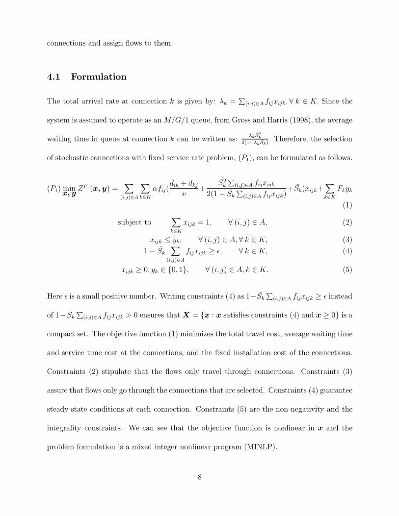
4.1 Formulation

The total arrival rate at connection k is given by: λk =∑

(i,j)∈A fijxijk, ∀ k ∈ K. Since the

system is assumed to operate as an M/G/1 queue, from Gross and Harris (1998), the average

waiting time in queue at connection k can be written as:λkS̄2

k

2(1−λkS̄k). Therefore, the selection

of stochastic connections with fixed service rate problem, (P1), can be formulated as follows:

(P1) minx, y

ZP1(x, y) =∑

(i,j)∈A

∑k∈K

αfij(dik + dkj

v+

S̄2k

∑(i,j)∈A fijxijk

2(1 − S̄k∑

(i,j)∈A fijxijk)+S̄k)xijk+

∑k∈K

Fkyk

(1)

subject to∑k∈K

xijk = 1, ∀ (i, j) ∈ A, (2)

xijk ≤ yk, ∀ (i, j) ∈ A, ∀ k ∈ K, (3)

1 − S̄k

∑(i,j)∈A

fijxijk ≥ ε, ∀ k ∈ K, (4)

xijk ≥ 0, yk ∈ {0, 1}, ∀ (i, j) ∈ A, k ∈ K. (5)

Here ε is a small positive number. Writing constraints (4) as 1−S̄k∑

(i,j)∈A fijxijk ≥ ε instead

of 1− S̄k∑

(i,j)∈A fijxijk > 0 ensures that X = {x : x satisfies constraints (4) and x ≥ 0} is a

compact set. The objective function (1) minimizes the total travel cost, average waiting time

and service time cost at the connections, and the fixed installation cost of the connections.

Constraints (2) stipulate that the flows only travel through connections. Constraints (3)

assure that flows only go through the connections that are selected. Constraints (4) guarantee

steady-state conditions at each connection. Constraints (5) are the non-negativity and the

integrality constraints. We can see that the objective function is nonlinear in x and the

problem formulation is a mixed integer nonlinear program (MINLP).

8

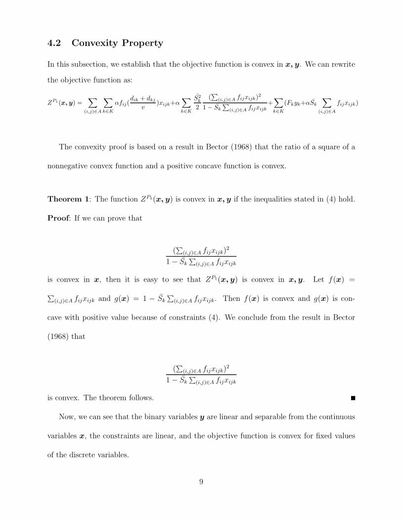
4.2 Convexity Property

In this subsection, we establish that the objective function is convex in x, y. We can rewrite

the objective function as:

ZP1(x, y) =∑

(i,j)∈A

∑k∈K

αfij(dik + dkj

v)xijk+α

∑k∈K

S̄2k

2

(∑

(i,j)∈A fijxijk)2

1 − S̄k

∑(i,j)∈A fijxijk

+∑k∈K

(Fkyk+αS̄k

∑(i,j)∈A

fijxijk)

The convexity proof is based on a result in Bector (1968) that the ratio of a square of a

nonnegative convex function and a positive concave function is convex.

Theorem 1: The function ZP1(x, y) is convex in x, y if the inequalities stated in (4) hold.

Proof: If we can prove that

(∑

(i,j)∈A fijxijk)2

1 − S̄k∑

(i,j)∈A fijxijk

is convex in x, then it is easy to see that ZP1(x, y) is convex in x, y. Let f(x) =

∑(i,j)∈A fijxijk and g(x) = 1 − S̄k

∑(i,j)∈A fijxijk. Then f(x) is convex and g(x) is con-

cave with positive value because of constraints (4). We conclude from the result in Bector

(1968) that

(∑

(i,j)∈A fijxijk)2

1 − S̄k∑

(i,j)∈A fijxijk

is convex. The theorem follows.

Now, we can see that the binary variables y are linear and separable from the continuous

variables x, the constraints are linear, and the objective function is convex for fixed values

of the discrete variables.

9

4.3 Outer Approximation Algorithm

As we mentioned before, the problem formulation (P1) is a mixed integer nonlinear optimiza-

tion problem (MINLP). Major algorithms for solving the MINLP problem include: branch

and bound (Beale (1977)), generalized Benders decomposition (GBD) (Geoffrion (1972)), and

outer approximation (OA) (Duran and Grossman (1986)). Other approximating methods

include: replacing the integer variables by continuous variables and approximating the non-

linear functions by linear functions. The combinatorial search techniques such as simulated

annealing and genetic algorithms have also been used to solve MINLP problems. Watkins

and McKinney (1998) believe that GBD and OA are better if binary variables y are linear

and separable from the continuous variables x, when both accuracy and computational time

are considered.

In this paper, the OA algorithm will be used to solve Problem (P1). The method can be

summarized as follows: It generates an upper bound and a lower bound at each iteration. The

upper bound results from the primal problem, which corresponds to the problem with fixed

integer variables. The lower bound results from the master problem. The master problem is

derived using primal information. As the iterations proceed, it is shown that the sequence of

updated upper-bounds is nonincreasing, the sequence of lower bounds is nondecreasing, and

that the sequence converge in a finite number of iterations. See Duran and Grossman (1986)

and Floudas (1995). The detail of the OA algorithm can be found in the Appendix. The

method is implemented through the use of the general algebraic modeling system (GAMS).

In Section 6.1, we provide some numerical results.

10

5 The Variable Service Rate Case

In this section, capacity is also determined through both the mean and second moment

(or variance) of service time at each connection. However, we assume that the mean and

second moment of service time at each connection are decision variables here. Changing the

mean of service time can be implemented by assigning workforce, machines (e.g., fork-lift

trucks in a distribution center), etc. Controlling variances is far more complicated than

changing the mean of service time. Often the variances encountered in a distribution center

can be the results of many factors in the system. These factors include distribution center

layout, use of warehouse management systems, automated storage and retrieval systems

(AS/RS), workforce training, scheduling, or demand forecasting, among others. For certain

applications, to control variance, these factors must be identified and controlled. See Melnyk,

Denzler, and Fredendall (1992) for more details.

We assume that the connection installation cost function includes two components: the

fixed cost related to the location, Fk, and the cost related to the capacity, c1/S̄k + c2/S̄2k ,

where c1 and c2 are constants. The fixed cost is related to connection location, for example,

the cost of leasing land. The latter is related to connection capacity. The estimation of c1

could be found by a regression analysis (for example, see Ashayeri, Gelders, and Wassenhove

(1985)). While we are not aware of existing literature that discusses the estimation of c2,

we believe that statistical techniques such as multifactor analysis of variance (ANOVA) and

multiple regression could be applied for this purpose. As noted earlier, it is generally more

difficult to reduce the variance than it is to reduce the mean, and we therefore expect c2 > c1.

The goal of this version of the problem is to locate some number of M/G/1 queueing

11

connections, allocate flows to them, and decide the service capacity at each selected connec-

tion.

5.1 Formulation

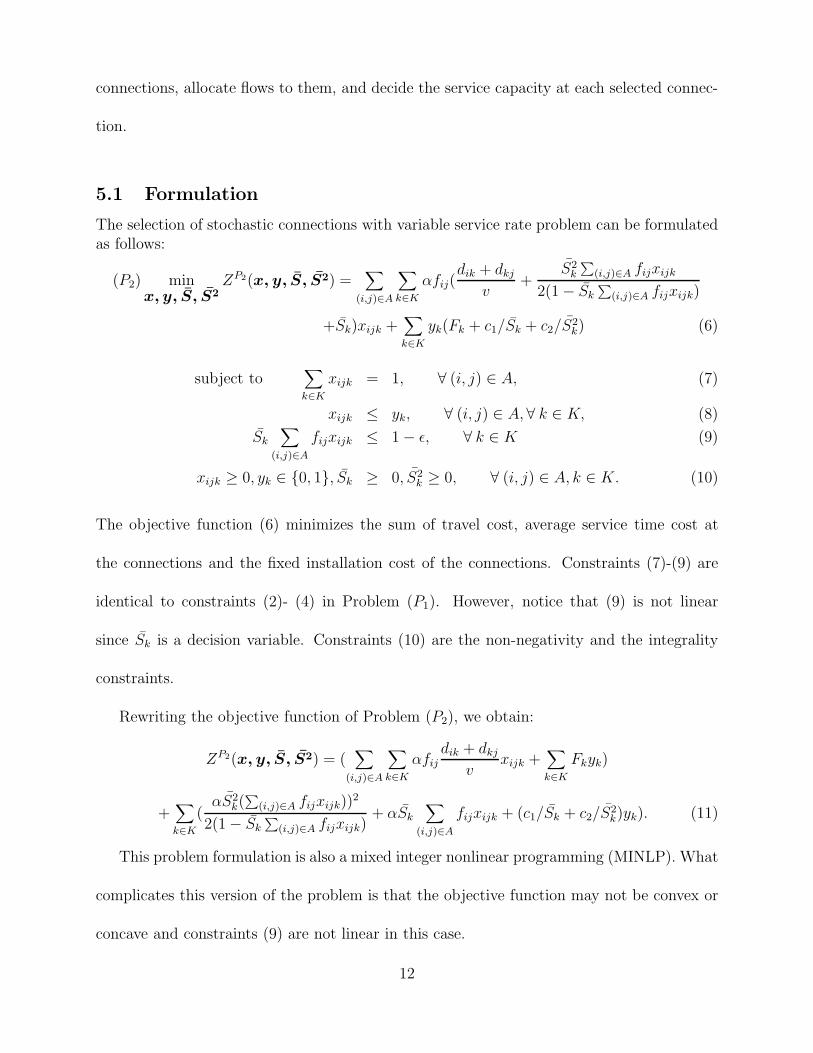
The selection of stochastic connections with variable service rate problem can be formulatedas follows:

(P2) minx, y, S̄, S̄2

ZP2(x, y, S̄, S̄2) =∑

(i,j)∈A

∑k∈K

αfij(dik + dkj

v+

S̄2k

∑(i,j)∈A fijxijk

2(1 − S̄k∑

(i,j)∈A fijxijk)

+S̄k)xijk +∑k∈K

yk(Fk + c1/S̄k + c2/S̄2k) (6)

subject to∑k∈K

xijk = 1, ∀ (i, j) ∈ A, (7)

xijk ≤ yk, ∀ (i, j) ∈ A, ∀ k ∈ K, (8)

S̄k

∑(i,j)∈A

fijxijk ≤ 1 − ε, ∀ k ∈ K (9)

xijk ≥ 0, yk ∈ {0, 1}, S̄k ≥ 0, S̄2k ≥ 0, ∀ (i, j) ∈ A, k ∈ K. (10)

The objective function (6) minimizes the sum of travel cost, average service time cost at

the connections and the fixed installation cost of the connections. Constraints (7)-(9) are

identical to constraints (2)- (4) in Problem (P1). However, notice that (9) is not linear

since S̄k is a decision variable. Constraints (10) are the non-negativity and the integrality

constraints.

Rewriting the objective function of Problem (P2), we obtain:

ZP2(x, y, S̄, S̄2) = (∑

(i,j)∈A

∑k∈K

αfijdik + dkj

vxijk +

∑k∈K

Fkyk)

+∑k∈K

(αS̄2

k(∑

(i,j)∈A fijxijk))2

2(1 − S̄k∑

(i,j)∈A fijxijk)+ αS̄k

∑(i,j)∈A

fijxijk + (c1/S̄k + c2/S̄2k)yk). (11)

This problem formulation is also a mixed integer nonlinear programming (MINLP). What

complicates this version of the problem is that the objective function may not be convex or

concave and constraints (9) are not linear in this case.

12

5.2 Properties

In this subsection we develop some key properties for the problem. These properties can

enable development of efficient solution methods.

5.2.1 The Equal Utilization Rate Property

The first property we seek to establish is that the utilization rates at the connections are

identical for an optimal solution to (P2). In order to do this, we take the following line of

attack:

• Define a subproblem (SP1) of (P2);

• Prove that (SP1) has equal utilization rate property;

• Prove that (P2) has equal utilization rate property.

Subproblem (SP1) Suppose that T is the total number of the selected connections in the

network. For simplicity, we assume that connections 1, 2, · · ·, T are selected. Each connection

is assumed to be an M/G/1 queueing system. Λ is the given total system flow, which is

equal to∑

(i,j)∈A fij. Let λk be the arrival rate at connection k, then∑k=T

k=1 λk = Λ. Let

ρk be the system utilization rate of connection k. Then ρk = λkS̄k. In order to prove the

equal utilization rate property, we use ρk and λk instead of S̄k and λk to formulate the cost

function. We now define the subproblem (SP1) of (P2) as follows:

(SP1) minρ, λ, S̄2

ZSP1(ρ, λ, S̄2) =k=T∑k=1

(αλ2

kS̄2k

2(1 − ρk)+ αρk +

c1λk

ρk+c2

S̄2k

) (12)

13

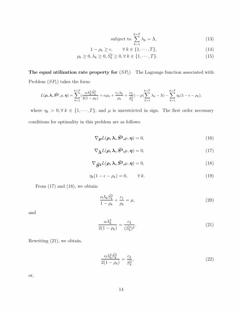
subject tok=T∑k=1

λk = Λ, (13)

1 − ρk ≥ ε, ∀ k ∈ {1, · · · , T}, (14)

ρk ≥ 0, λk ≥ 0, S̄2k ≥ 0, ∀ k ∈ {1, · · · , T}. (15)

The equal utilization rate property for (SP1) The Lagrange function associated with

Problem (SP1) takes the form:

L(ρ, λ, S̄2, µ, η) =k=T∑k=1

(αλ2

kS̄2k

2(1 − ρk)+ αρk +

c1λk

ρk+

c2

S̄2k

) − µ(k=T∑k=1

λk − Λ) −k=T∑k=1

ηk(1 − ε − ρk),

where ηk > 0, ∀ k ∈ {1, · · · , T}, and µ is unrestricted in sign. The first order necessary

conditions for optimality in this problem are as follows:

∇ρL(ρ, λ, S̄2,µ,η) = 0, (16)

∇λL(ρ, λ, S̄2,µ,η) = 0, (17)

∇S̄2L(ρ, λ, S̄2,µ,η) = 0, (18)

ηk(1 − ε− ρk) = 0, ∀ k. (19)

From (17) and (18), we obtain:

αλkS̄2k

1 − ρk+c1ρk

= µ, (20)

and

αλ2k

2(1 − ρk)=

c2

(S̄2k)

2. (21)

Rewriting (21), we obtain,

αλ2kS̄

2k

2(1 − ρk)=c2

S̄2k

, (22)

or,

14

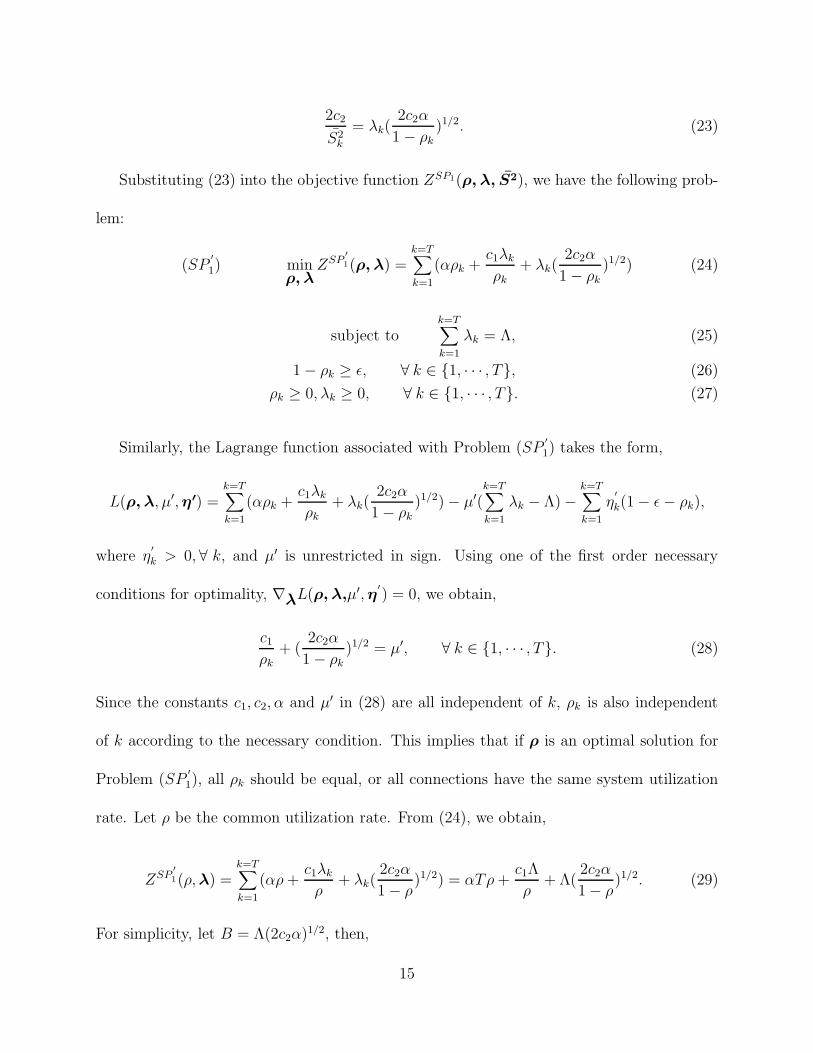
2c2

S̄2k

= λk(2c2α

1 − ρk)1/2. (23)

Substituting (23) into the objective function ZSP1(ρ, λ, S̄2), we have the following prob-

lem:

(SP′1) min

ρ, λZSP

′1(ρ, λ) =

k=T∑k=1

(αρk +c1λk

ρk

+ λk(2c2α

1 − ρk

)1/2) (24)

subject tok=T∑k=1

λk = Λ, (25)

1 − ρk ≥ ε, ∀ k ∈ {1, · · · , T}, (26)

ρk ≥ 0, λk ≥ 0, ∀ k ∈ {1, · · · , T}. (27)

Similarly, the Lagrange function associated with Problem (SP′1) takes the form,

L(ρ, λ, µ′,η′) =k=T∑k=1

(αρk +c1λk

ρk+ λk(

2c2α

1 − ρk)1/2) − µ′(

k=T∑k=1

λk − Λ) −k=T∑k=1

η′k(1 − ε− ρk),

where η′k > 0, ∀ k, and µ′ is unrestricted in sign. Using one of the first order necessary

conditions for optimality, ∇λL(ρ, λ,µ′,η′) = 0, we obtain,

c1ρk

+ (2c2α

1 − ρk)1/2 = µ′, ∀ k ∈ {1, · · · , T}. (28)

Since the constants c1, c2, α and µ′ in (28) are all independent of k, ρk is also independent

of k according to the necessary condition. This implies that if ρ is an optimal solution for

Problem (SP′1), all ρk should be equal, or all connections have the same system utilization

rate. Let ρ be the common utilization rate. From (24), we obtain,

ZSP′1(ρ,λ) =

k=T∑k=1

(αρ+c1λk

ρ+ λk(

2c2α

1 − ρ)1/2) = αTρ+

c1Λ

ρ+ Λ(

2c2α

1 − ρ)1/2. (29)

For simplicity, let B = Λ(2c2α)1/2, then,

15

ZSP′1(ρ,λ) = Z(ρ) = αTρ+

c1Λ

ρ+

B

(1 − ρ)1/2. (30)

From (30), the optimal objective value of Problem (SP′1) can be decided only by ρ. How

to find optimal ρ will be discussed in Section 5.2.2. Notice that λk does not appear in the

objective function but Λ(=∑k=T

k=1 λk) does. Therefore, the optimal solution for Problem

(SP′1) is not unique. In fact, suppose that ρ∗ is optimal solution from (30), then for any

given λk such that∑k=T

k=1 λk = Λ, the solution (ρ∗, λ) is optimal to Problem (SP′1).

Thus, the optimal solution of Problem (SP1) can be found by solving Problem (SP′1) to

obtain a solution for ρ, λ and (23) to obtain S̄2.

The equal utilization rate property for Problem (P2) Recalling that ZP2(x, y, S̄, S̄2)

(see (11)) includes the following two types of costs:

∑(i,j)∈A

∑k∈K

αfijdik + dkj

vxijk +

∑k∈K

Fkyk

and

∑k∈K

(αS̄2

k(∑

(i,j)∈A fijxijk))2

2(1 − S̄k∑

(i,j)∈A fijxijk)+ αS̄k

∑(i,j)∈A

fijxijk + (c1/S̄k + c2/S̄2k)yk).

The first is a “fixed charge facility location” type of cost. Since λk =∑

(i,j)∈A fijxijk, the

second one is the objective function of Problem (SP1) when connection locations are fixed. In

fact, by the discussion above, this cost can be determined without specifying exact connection

locations as long as the total number of selected connections is determined, i.e.,∑

k∈K yk.

Now we prove the following theorem.

Theorem 2: The utilization rates at the connections are identical for an optimal solution

to Problem (P2).

16

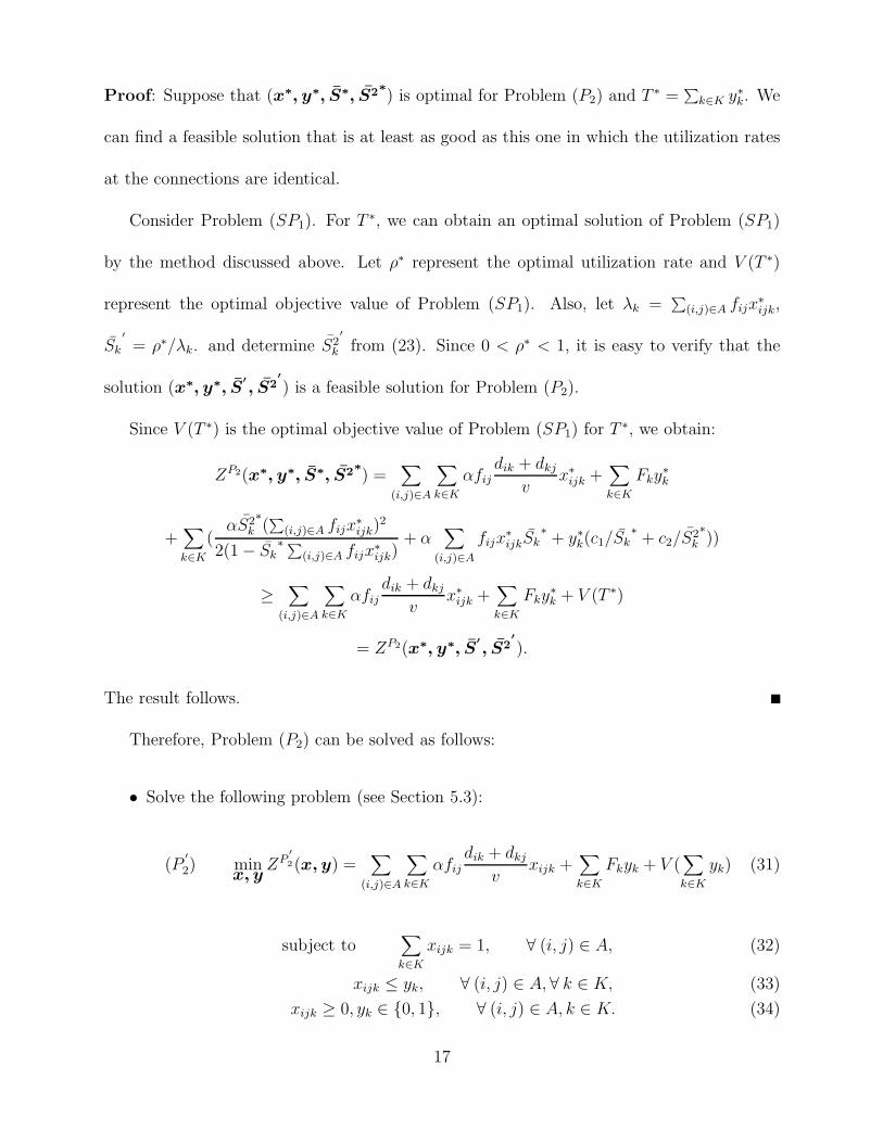
Proof: Suppose that (x∗, y∗, S̄∗, S̄2∗) is optimal for Problem (P2) and T ∗ =

∑k∈K y∗k. We

can find a feasible solution that is at least as good as this one in which the utilization rates

at the connections are identical.

Consider Problem (SP1). For T ∗, we can obtain an optimal solution of Problem (SP1)

by the method discussed above. Let ρ∗ represent the optimal utilization rate and V (T ∗)

represent the optimal objective value of Problem (SP1). Also, let λk =∑

(i,j)∈A fijx∗ijk,

S̄k

′= ρ∗/λk. and determine S̄2

k

′from (23). Since 0 < ρ∗ < 1, it is easy to verify that the

solution (x∗, y∗, S̄′, S̄2

′) is a feasible solution for Problem (P2).

Since V (T ∗) is the optimal objective value of Problem (SP1) for T ∗, we obtain:

ZP2(x∗, y∗, S̄∗, S̄2∗) =

∑(i,j)∈A

∑k∈K

αfijdik + dkj

vx∗ijk +

∑k∈K

Fky∗k

+∑k∈K

(αS̄2

k

∗(∑

(i,j)∈A fijx∗ijk)

2

2(1 − S̄k∗ ∑

(i,j)∈A fijx∗ijk)+ α

∑(i,j)∈A

fijx∗ijkS̄k

∗+ y∗k(c1/S̄k

∗+ c2/S̄2

k

∗))

≥ ∑(i,j)∈A

∑k∈K

αfijdik + dkj

vx∗ijk +

∑k∈K

Fky∗k + V (T ∗)

= ZP2(x∗, y∗, S̄′, S̄2

′).

The result follows.

Therefore, Problem (P2) can be solved as follows:

• Solve the following problem (see Section 5.3):

(P′2) min

x, yZP

′2(x, y) =

∑(i,j)∈A

∑k∈K

αfijdik + dkj

vxijk +

∑k∈K

Fkyk + V (∑k∈K

yk) (31)

subject to∑k∈K

xijk = 1, ∀ (i, j) ∈ A, (32)

xijk ≤ yk, ∀ (i, j) ∈ A, ∀ k ∈ K, (33)

xijk ≥ 0, yk ∈ {0, 1}, ∀ (i, j) ∈ A, k ∈ K. (34)

17

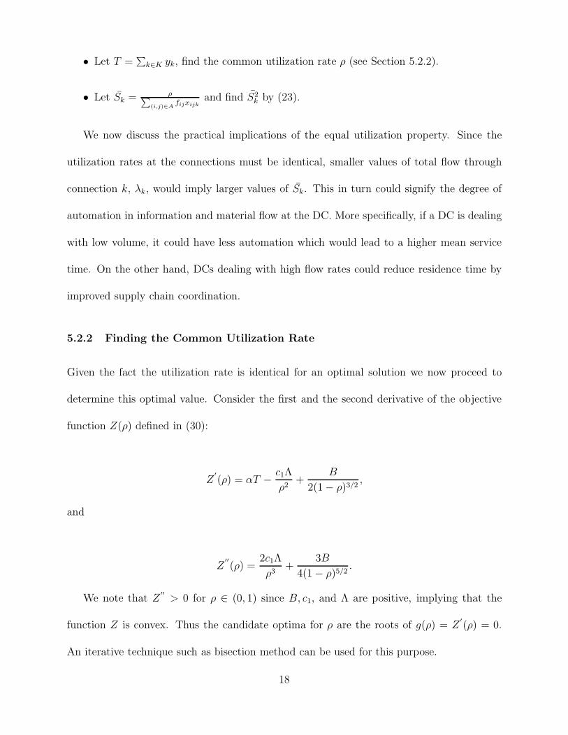
• Let T =∑

k∈K yk, find the common utilization rate ρ (see Section 5.2.2).

• Let S̄k = ρ∑(i,j)∈A

fijxijkand find S̄2

k by (23).

We now discuss the practical implications of the equal utilization property. Since the

utilization rates at the connections must be identical, smaller values of total flow through

connection k, λk, would imply larger values of S̄k. This in turn could signify the degree of

automation in information and material flow at the DC. More specifically, if a DC is dealing

with low volume, it could have less automation which would lead to a higher mean service

time. On the other hand, DCs dealing with high flow rates could reduce residence time by

improved supply chain coordination.

5.2.2 Finding the Common Utilization Rate

Given the fact the utilization rate is identical for an optimal solution we now proceed to

determine this optimal value. Consider the first and the second derivative of the objective

function Z(ρ) defined in (30):

Z′(ρ) = αT − c1Λ

ρ2+

B

2(1 − ρ)3/2,

and

Z′′(ρ) =

2c1Λ

ρ3+

3B

4(1 − ρ)5/2.

We note that Z′′> 0 for ρ ∈ (0, 1) since B, c1, and Λ are positive, implying that the

function Z is convex. Thus the candidate optima for ρ are the roots of g(ρ) = Z′(ρ) = 0.

An iterative technique such as bisection method can be used for this purpose.

18

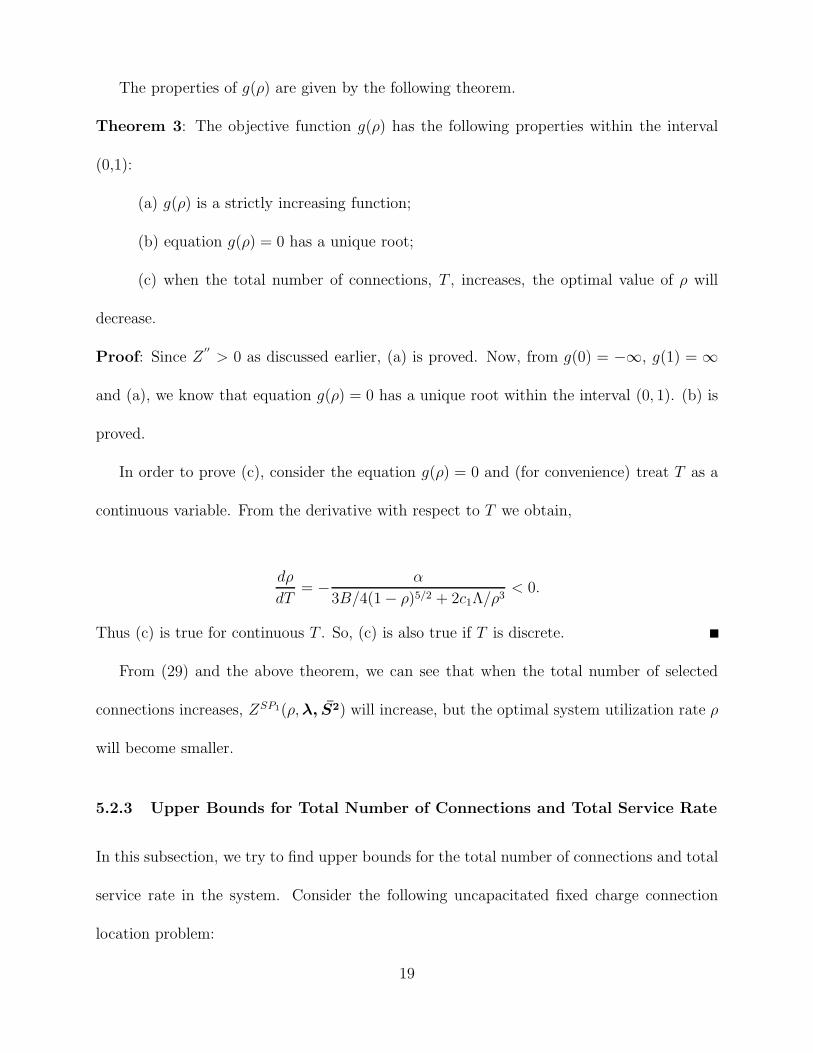
The properties of g(ρ) are given by the following theorem.

Theorem 3: The objective function g(ρ) has the following properties within the interval

(0,1):

(a) g(ρ) is a strictly increasing function;

(b) equation g(ρ) = 0 has a unique root;

(c) when the total number of connections, T , increases, the optimal value of ρ will

decrease.

Proof: Since Z′′> 0 as discussed earlier, (a) is proved. Now, from g(0) = −∞, g(1) = ∞

and (a), we know that equation g(ρ) = 0 has a unique root within the interval (0, 1). (b) is

proved.

In order to prove (c), consider the equation g(ρ) = 0 and (for convenience) treat T as a

continuous variable. From the derivative with respect to T we obtain,

dρ

dT= − α

3B/4(1 − ρ)5/2 + 2c1Λ/ρ3< 0.

Thus (c) is true for continuous T . So, (c) is also true if T is discrete.

From (29) and the above theorem, we can see that when the total number of selected

connections increases, ZSP1(ρ,λ, S̄2) will increase, but the optimal system utilization rate ρ

will become smaller.

5.2.3 Upper Bounds for Total Number of Connections and Total Service Rate

In this subsection, we try to find upper bounds for the total number of connections and total

service rate in the system. Consider the following uncapacitated fixed charge connection

location problem:

19

(SP2) minx, y

ZSP2(x, y) =∑

(i,j)∈A

∑k∈K

αfijdik + dkj

vxijk +

∑k∈K

Fkyk (35)

subject to∑k∈K

xijk = 1, ∀ (i, j) ∈ A, (36)

xijk ≤ yk, ∀ (i, j) ∈ A, ∀ k ∈ K, (37)

xijk ≥ 0, yk ∈ {0, 1}, ∀ (i, j) ∈ A, k ∈ K. (38)

Let (x∗, y∗) be the optimal solution for Problem (SP2) and T ∗ =∑

k∈K y∗k, then, we have

the following theorem.

Theorem 4: The upper bound for total number of connections in Problem (P2) is T ∗.

Proof: Consider Problem (P′2). Since (x∗, y∗) is the optimal solution for Problem (SP2),

opening one more connections will not decrease the objective value of Problem (SP2). On

the other hand, from (30), we know that V (T ) is an increasing function of T . Verifying (31),

the result follows.

Let ρ∗ be the optimal utilization rate for this T ∗. From Theorem 4 (c), we have the following

corollary:

Corollary 1: ρ∗ is the lower bound for the optimal utilization rate of Problem (P2).

Since V (∑

k∈K yk) in Problem (P′2) is not affected by λ, S̄2, we can always find the average

service time S̄k or the average service rate 1/S̄k by S̄k = ρ/∑

(i,j)∈A fijxijk. Thus,

∑k∈K

1

S̄k

=∑k∈K

∑(i,j)∈A fijxijk

ρ=

∑k∈K

∑(i,j)∈A fijxijk

ρ=

Λ

ρ

where Λ =∑

(i,j)∈A fij is the given total system flows. Thus we obtain:

Corollary 2: The upper bound for the optimal total service rate of Problem (P2) is Λ/ρ∗.

20

Corollary 3: If ρ∗ is the optimal utilization rate of Problem (P2), Λ/ρ∗ is the optimal total

service rate of Problem (P2).

5.3 Lagrangian Relaxation Algorithm

In this section, based on some of the previous properties, we develop a Lagrangian relaxation

algorithm to solve Problem (P′2). Let (LRP ) be the Lagrangian relaxation problem corre-

sponding to relaxing the assignment constraints (32) for a given set of Lagrangian multipliers

µ.

(LRP ) minx, y

ZLRP (µ) =∑

(i,j)∈A

∑k∈K

αfijdik + dkj

vxijk +

∑k∈K

ykFk +V (∑k∈K

yk)+∑

(i,j)∈A

µij(1−∑k∈K

xijk) (39)

subject to (33) and (34).

The objective function of (LRP )(µ) can be rewritten as:

(LRP ) minx, y

ZLRP (µ) =∑k∈K

∑(i,j)∈A

(αfijdik + dkj

v− µij)xijk +

∑k∈K

ykFk + V (∑k∈K

yk) +∑

(i,j)∈A

µij . (40)

The ideal choice of multipliers is such that they solve the Lagrangian dual problem, denoted

by (DP ):

(DP ) maxµ

ZDP (µ) (41)

The optimal value of the above problem (DP ) provides the “best” lower bound (using the

Lagrangian method).

For fixed values of the Lagrange multipliers µ, the optimal solution for (LRP ) can be

obtained by the following method:

Calculate pk = Fk +∑

(i,j)∈A min{0, (αfijdik+dkj

v− µij)} for each k. Sort pk in increasing

21

order and let pk1 , pk2, · · · be the sequence after sorting, so that pk1 ≤ pk2 ≤ · · ·. Let

∆V (T ) =

⎧⎪⎪⎪⎪⎪⎨⎪⎪⎪⎪⎪⎩

V (0), if T = 0,

V (T ) − V (T − 1), if T > 0

From the Section 5.2.2, ∆V (T ) ≥ 0. The optimal y value can be obtained by the following

procedure:

Set yk1 = 1;

For j = 2 to |K|,

set ykj= 1, if pkj

+ ∆V (j) < 0;

set ykj= 0, otherwise.

The corresponding optimal x value is

xijk =

⎧⎪⎪⎪⎪⎪⎨⎪⎪⎪⎪⎪⎩

1, if yk = 1 and αfijdik+dkj

v− µij < 0

0, otherwise.

If the solution for the relaxed problem is feasible to the original problem, we compute and

update the upper bound of the original problem. If it is not, i.e., some flows are assigned to

more than one connection or some flows are not assigned to any connection, we can construct

a primal feasible solution by simply opening connections with yk = 1 and assigning flows

to their closest connections. The primal objective will provide us with an upper bound on

the solution. If the termination conditions are satisfied, we stop. Otherwise, we decide if

we need to update the Lagrange multipliers µij. If we decide to terminate the Lagrangian

procedure, the best upper bound gives us a heuristic solution. The following is a step-by-step

description of the procedure:

Step 0. Prepare V (T ) and ∆V (T ) for T ∈ K.

22

Step 1. Relax constraints (32), fix the initial µij (we arbitrarily choose µij=1 here);

Step 2. Solve (LRP ), compute and update the lower bound;

Step 3. If the solution for the relaxed problem is feasible to (P′2), update the upper bound; if

not, find a feasible solution by the method mentioned above, then update the upper

bound;

Step 4. If the termination conditions are satisfied, stop; otherwise, update µij (see Fisher

(1981)), and go to Step 2.

6 Computational Performance

In this section, we present the results of randomly generated problems for both cases. We first

generated each node’s location, which was decided by its x-coordinate and the y-coordinate.

These coordinate values were randomly selected from U(0, 1000), where U denotes a uniform

distribution. The candidate sites of connections were also decided by its x-coordinate and the

y-coordinate, where the x-coordinate values and y-coordinate values were randomly selected

from the minimum value of the x-coordinate and the y-coordinate values of node’s location

to maximum value of x-coordinate and the y-coordinate values of node’s location. For each

pair of distinct nodes, the amount of flow was randomly drawn from U(5, 30). Fk is randomly

selected from U(3000, 5000). We assume α = 1 and v = 1 in both cases. To demonstrate

the performance of the algorithms, we use both “heuristic gap” and CPU time to evaluate

the efficiency of our algorithm. Heuristic gap is defined as (best upper bound - best lower

bound)/best lower bound * 100. Using this term, we can guarantee that the solution for the

23

original problem is near-optimal if the heuristic gap is very small.

6.1 OA Algorithm

In the fixed service rate case, we need to generate the mean service time S̄k and the second

moment of service time S̄2k . Let ψ =

∑(i,j)∈A fij/|K|, where |K| is the total number of

candidate connection sites and ψ is the average flow for the total number of candidate

connection sites. The service rate 1/S̄k is randomly selected from U(3ψ, 4ψ). We let S̄2k =

2S̄k. The OA algorithm was implemented through the use of GAMS using its default settings.

The MILP solver used was CPLEX, and the NLP solver was CONOPT2. The procedure

stops as soon as the bound defined by the objective of the last MILP master problem is

worse than the best NLP solution found (a “crossover” occurred) or the number of cycles is

greater than 50.

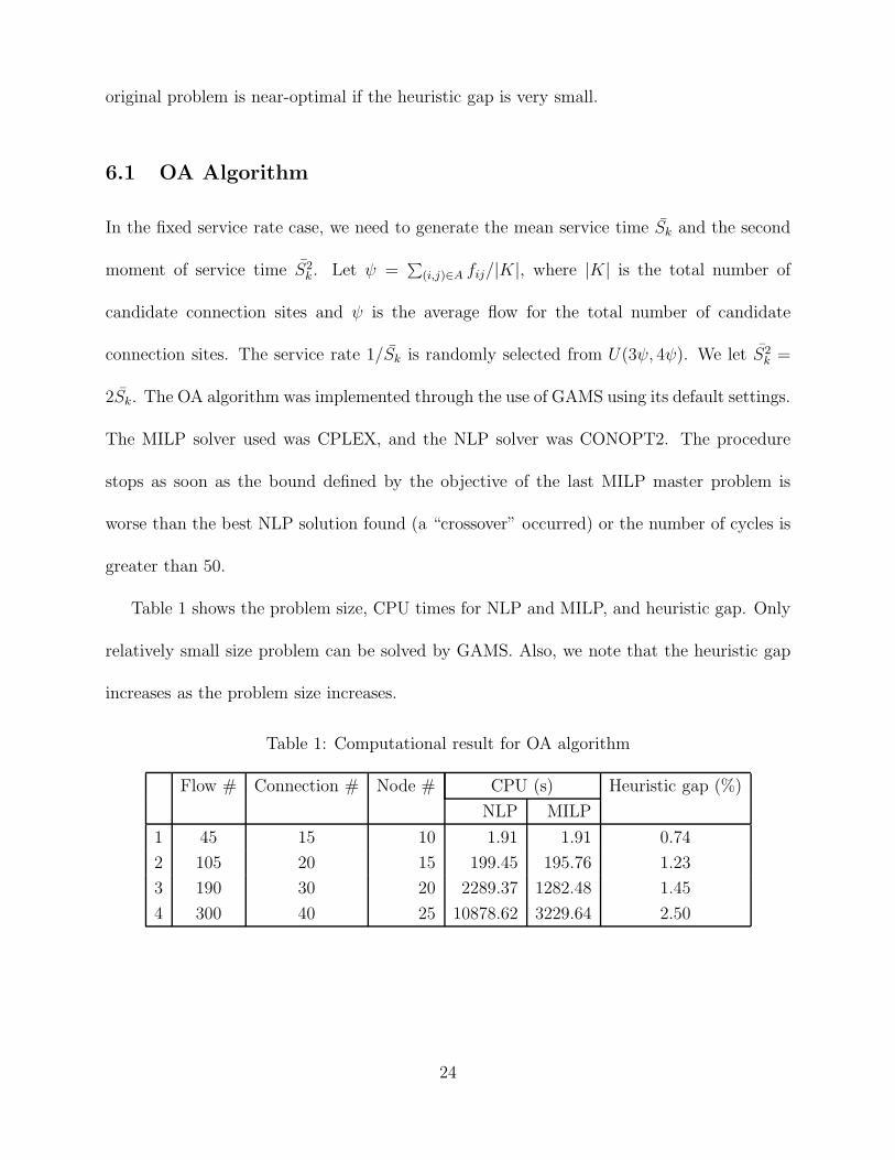
Table 1 shows the problem size, CPU times for NLP and MILP, and heuristic gap. Only

relatively small size problem can be solved by GAMS. Also, we note that the heuristic gap

increases as the problem size increases.

Table 1: Computational result for OA algorithm

Flow # Connection # Node # CPU (s) Heuristic gap (%)

NLP MILP

1 45 15 10 1.91 1.91 0.74

2 105 20 15 199.45 195.76 1.23

3 190 30 20 2289.37 1282.48 1.45

4 300 40 25 10878.62 3229.64 2.50

24

6.2 Lagrangian Relaxation Algorithm

In the variable service rate case, we arbitrarily choose c1 = 1 and c2 = 1. The bisection

method is used to find V (T ) for each T . We terminate the procedure if the heuristic gap is

less than 0.0001 or after 1000 iterations. The algorithm is coded in C++.

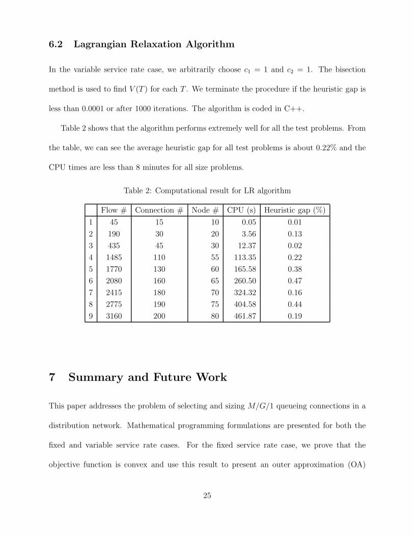
Table 2 shows that the algorithm performs extremely well for all the test problems. From

the table, we can see the average heuristic gap for all test problems is about 0.22% and the

CPU times are less than 8 minutes for all size problems.

Table 2: Computational result for LR algorithm

Flow # Connection # Node # CPU (s) Heuristic gap (%)

1 45 15 10 0.05 0.01

2 190 30 20 3.56 0.13

3 435 45 30 12.37 0.02

4 1485 110 55 113.35 0.22

5 1770 130 60 165.58 0.38

6 2080 160 65 260.50 0.47

7 2415 180 70 324.32 0.16

8 2775 190 75 404.58 0.44

9 3160 200 80 461.87 0.19

7 Summary and Future Work

This paper addresses the problem of selecting and sizing M/G/1 queueing connections in a

distribution network. Mathematical programming formulations are presented for both the

fixed and variable service rate cases. For the fixed service rate case, we prove that the

objective function is convex and use this result to present an outer approximation (OA)

25

algorithm. The algorithm was implemented through the use of GAMS. For the variable

service rate case, we establish that the utilization rates at the connections are identical

for an optimal solution. Based on this key property, we develop a Lagrangian relaxation

algorithm. Compared to the OA algorithm, this algorithm performs very well under both

the accuracy and CPU time criteria. A useful extension to the work presented in this paper

would be to modify the models and solution approaches to treat capacity as a set of discrete

options. Modeling the connections as M/G/k queueing systems could be another challenging

extension.

Appendix

The OA algorithm as applied to the problem (P1) can be stated as follows:

Step 1 : Select initial values for variables y, say, y1 = 1. Set the counter m = 1 and the

current upper bound UBD = +∞. Choose the convergence tolerance δ.

Step 2 : Solve the primal problem PP :

(PP ) minx

ZPP (x) =∑

(i,j)∈A

∑k∈K

αfij(dik + dkj

v+

S̄2k

∑(i,j)∈A fijxijk

2(1 − S̄k∑

(i,j)∈A fijxijk)+S̄k)xijk+

∑k∈K

Fkymk

subject to∑k∈K

xijk = 1, ∀ (i, j) ∈ A,

xijk ≤ ymk , ∀ (i, j) ∈ A, ∀ k ∈ K,

1 − S̄k

∑(i,j)∈A

fijxijk ≥ ε, ∀ k ∈ K,

xijk ≥ 0, ∀ (i, j) ∈ A, k ∈ K.

It gives an optimal primal solution xm and an optimal value of objective function

Z(xm,ym). Update the current upper bound UBD = min{UBD,Z(xm,ym)}. If

26

UBD = Z(xm,ym), set y∗ = ym and x∗ = xm, where x∗,y∗ is the current best

solution.

Step 3 : Solve the following master problem:

(MP ) miny,η

ZMP (y, η) = η +∑k∈K

Fkyk

subject to η ≥ f(xm) + ∇f(xm)T (x − xm), ∀m ∈ {1, 2, · · ·,M},∑k∈K

xijk = 1, ∀ (i, j) ∈ A,

xijk ≤ yk, ∀ (i, j) ∈ A, ∀ k ∈ K,

1 − S̄k

∑(i,j)∈A

fijxijk ≥ ε, ∀ k ∈ K,

η ∈ R1, xijk ≥ 0, yk ∈ {0, 1}, ∀ (i, j) ∈ A, k ∈ K.

Where f(x) =∑

(i,j)∈A

∑k∈K αfij(

dik+dkj

v+

S̄2k

∑(i,j)∈A

fijxijk

2(1−S̄k

∑(i,j)∈A

fijxijk)+ S̄k)xijk. The solution

of the master problem gives ym+1 and ZMP , where ZMP is a lower bound on the

objective function of (P1). If (UBD − ZMP )/UBD ≤ ε, stop, the solution is x∗,y∗;

otherwise, set m = m+ 1 and return to step 2.

Acknowledgments

The authors would like to acknowledge support from the National Science Foundation via

Grant No. DMI-0300370.

27

References

Ashayeri, J., L. F. Gelders, and L. V. Wassenhove (1985). A microcomputer-based opti-

mization model for the design of automated warehouses. International Journal of Pro-

duction Research 23, 825–839.

Aykin, T. (1994). Lagrangian relaxation based approaches to capacitated hub-and-spoke

network design problem. European Journal of Operational Research 79, 501–523.

Batta, R., A. Ghose, and U. S. Palekar (1989). Locating facilities on the Manhattan metric

with arbitrary shaped barriers and convex forbidden regions. Transportation Science 23,

26–36.

Beale, E. M. L. (1977). Integer programming. In D. Jacobs (Ed.), The State of the Art in

Numerical Analysis, pp. 409. Academic Press.

Bector, C. R. (1968). Programming problems with convex fractional functions. Operations

Research 16, 383–391.

Berman, O. and R. C. Larson (1982). The median problem with congestion. Computers

and Operations Research 9, 119–126.

Berman, O., R. C. Larson, and N. Fouska (1992). Optimal location of discretionary service

facilities. Transportation Science 26, 201–211.

Berman, O., R. C. Larson, and C. Parkan (1987). The stochastic queue p-median problem.

Transportation Science 21, 207–216.

Bitran, G. B. and D. Tirupati (1989). Tradeoff curves, targeting and balancing in manu-

facturing queueing networks. Operations Research 37, 547–564.

28

Bretthauer, K. M. (1995). Capacity planning in networks of queues with manufacturing

applications. Mathl. Comput. Modelling 21, 35–46.

Brimberg, J. and A. Mehrez (1997). A note on the allocation of queueing facilities using

a minisum criterion. Journal of the Operational Research Society 48, 195–201.

Brimberg, J., A. Mehrez, and G. O. Wesolowsky (1997). Allocation of queueing facilities

using a minimax criterion. Location Science 5, 89–101.

Campbell, J. F. (1994). Integer programming formulations of discrete hub location prob-

lems. European Journal of Operational Research 72, 387–405.

Crabill, T. B., D. Gross, and M. J. Magazine (1977). A classified bibliography of research

on optimal design and control of queues. Operations Research 25, 219–232.

Duran, M. A. and I. E. Grossman (1986). An outer approximation algorithm for a class

of mixed-integer nonlinear programs. Mathematical Programming 36, 307–339.

Ebery, J., M. Krishnamoorthy, A. Ernst, and N. Boland (2000). The capacitated multi-

ple allocation hub location problem: Formulations and algorithms. European Journal of

Operational Research 120, 614–631.

Enns, S. T. (1998). Work flow analysis using queuing decomposition models. Computers

and Industrial Engineering 34, 371–383.

Fisher, M. L. (1981). The lagrangian relaxation method for solving integer programming

problem. Management Science 27, 1–18.

Floudas, C. A. (1995). Nonlinear and Mixed-Integer Optimization: Fundamentals and

Applications. Oxford University Press, New York.

29

Geoffrion, A. M. (1972). Generalized benders decomposition. J. Opt. Theory and Appl. 10,

237–260.

Gross, D. and C. M. Harris (1998). Fundamentals of Queueing Theory, 3rd Edition. John

Wiley, New York.

Hillier, F. S. and K. C. So (1991). The effect of the coefficient of variation of operation

times on the allocation of storage space in production line systems. IIE Transactions 23,

198–206.

Hodgon, M. J. (1990). A flow-capturing location-allocation model. Geographical Analy-

sis 22, 270–279.

Huang, S., R. Batta, and R. Nagi (2003). Variable capacity sizing and selection of con-

nections in a facility layout. IIE Transactions 35, 49–59.

Marianov, V. (2003). Location of multiple-server congestible facilities for maximizing ex-

pected demand when services are non-essential. Annals of Operations Research 123, 125–

141.

Melnyk, S. A., D. R. Denzler, and L. Fredendall (1992). Variance control vs. dispatching

efficiency. Production and Inventory Management Journal Third Quarter, 6–13.

O’Kelly, M. (1986). The location of interacting hub facilities. Transportation Science 20,

92–106.

Park, C. S. (2002). Contemporary Engineering Economics, 3rd Edition. Prentice-Hall, NJ.

Shanthikumar, J. D. and D. D. Yao (1988). On server allocation in multiple center man-

ufacturing systems. Operations Research 36, 333–342.

30

Stidham, S. (2002). Analysis, design, and control of queueing systems. Operations Re-

search 50, 197–216.

Wang, Q., R. Batta, and C. M. Rump (2002). Algorithms for a facility location prob-

lem with stochastic customer demand and immobile servers. Annals of Operations Re-

search 111, 17–34.

Watkins, D. W. and D. C. McKinney (1998). Decomposition methods for water resources

optimization models with fixed costs. Advances in Water Resources 21, 283–295.

Yamazaki, G., H. Sakasegawa, and J. G. Shanthikumar (1992). On the optimal arrange-

ment of stations in tandem queueing system with blocking. Management Science 39,

137–153.

Yao, D. D. and S. C. Kim (1987). Reducing the congestion in a class of job shops. Man-

agement Science 34, 1165–1172.

31