Distributed OLAP Databases - CMU 15-445/645 · SALES_FACT PRODUCT_FK TIME_FK LOCATION_FK...
46
Database Systems 15-445/15-645 Fall 2018 Andy Pavlo Computer Science Carnegie Mellon Univ. AP Lecture #24 Distributed OLAP Databases
Transcript of Distributed OLAP Databases - CMU 15-445/645 · SALES_FACT PRODUCT_FK TIME_FK LOCATION_FK...
Database Systems
15-445/15-645
Fall 2018
Andy PavloComputer Science Carnegie Mellon Univ.AP
Lecture #24
Distributed OLAP Databases
CMU 15-445/645 (Fall 2018)
UPCOMING DATABASE EVENTS
Swarm64 Tech Talk→ Thursday November 29th @ 12pm→ GHC 8102 ← Different Location!
VoltDB Research Talk→ Monday December 3rd @ 4:30pm→ GHC 8102
2
CMU 15-445/645 (Fall 2018)
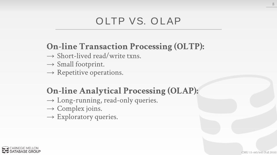
OLTP VS. OL AP
On-line Transaction Processing (OLTP):→ Short-lived read/write txns.→ Small footprint.→ Repetitive operations.
On-line Analytical Processing (OLAP):→ Long-running, read-only queries.→ Complex joins.→ Exploratory queries.
8
CMU 15-445/645 (Fall 2018)
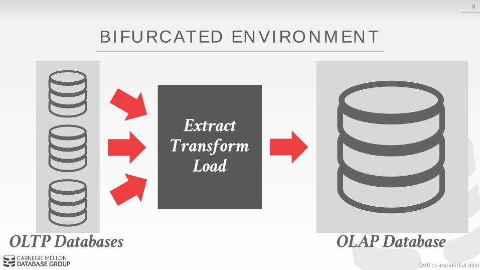
BIFURCATED ENVIRONMENT
9
ExtractTransform
Load
OLAP DatabaseOLTP Databases
CMU 15-445/645 (Fall 2018)
DECISION SUPPORT SYSTEMS
Applications that serve the management, operations, and planning levels of an organization to help people make decisions about future issues and problems by analyzing historical data.
Star Schema vs. Snowflake Schema
10
CMU 15-445/645 (Fall 2018)
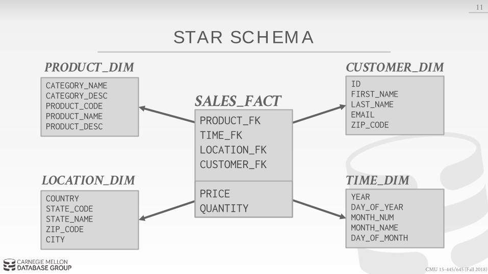
STAR SCHEMA
11
CATEGORY_NAMECATEGORY_DESCPRODUCT_CODEPRODUCT_NAMEPRODUCT_DESC
PRODUCT_DIM
COUNTRYSTATE_CODESTATE_NAMEZIP_CODECITY
LOCATION_DIM
IDFIRST_NAMELAST_NAMEEMAILZIP_CODE
CUSTOMER_DIM
YEARDAY_OF_YEARMONTH_NUMMONTH_NAMEDAY_OF_MONTH
TIME_DIM
SALES_FACTPRODUCT_FKTIME_FKLOCATION_FKCUSTOMER_FK
PRICEQUANTITY
CMU 15-445/645 (Fall 2018)
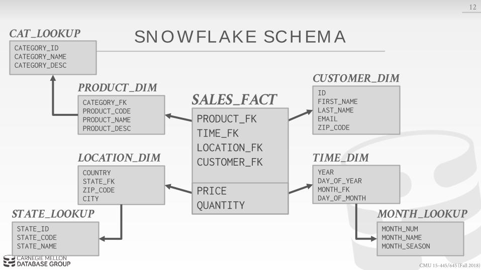
SNOWFL AKE SCHEMA
12
CATEGORY_FKPRODUCT_CODEPRODUCT_NAMEPRODUCT_DESC
PRODUCT_DIM
COUNTRYSTATE_FKZIP_CODECITY
LOCATION_DIM
IDFIRST_NAMELAST_NAMEEMAILZIP_CODE
CUSTOMER_DIM
YEARDAY_OF_YEARMONTH_FKDAY_OF_MONTH
TIME_DIM
SALES_FACTPRODUCT_FKTIME_FKLOCATION_FKCUSTOMER_FK
PRICEQUANTITY
CATEGORY_IDCATEGORY_NAMECATEGORY_DESC
CAT_LOOKUP
STATE_IDSTATE_CODESTATE_NAME
STATE_LOOKUPMONTH_NUMMONTH_NAMEMONTH_SEASON
MONTH_LOOKUP
CMU 15-445/645 (Fall 2018)
STAR VS. SNOWFL AKE SCHEMA
Issue #1: Normalization→ Snowflake schemas take up less storage space.→ Denormalized data models may incur integrity and
consistency violations.
Issue #2: Query Complexity→ Snowflake schemas require more joins to get the data
needed for a query.→ Queries on star schemas will (usually) be faster.
13
CMU 15-445/645 (Fall 2018)
P3 P4
P1 P2
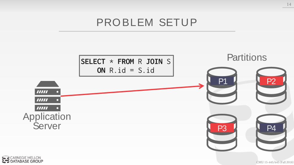
PROBLEM SETUP
14
ApplicationServer
PartitionsSELECT * FROM R JOIN SON R.id = S.id
CMU 15-445/645 (Fall 2018)
P3 P4
P1 P2
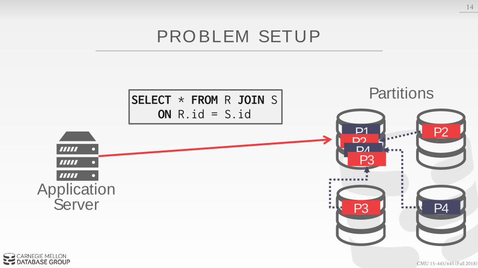
PROBLEM SETUP
14
ApplicationServer
PartitionsSELECT * FROM R JOIN SON R.id = S.id
P2P4P3
CMU 15-445/645 (Fall 2018)
TODAY'S AGENDA
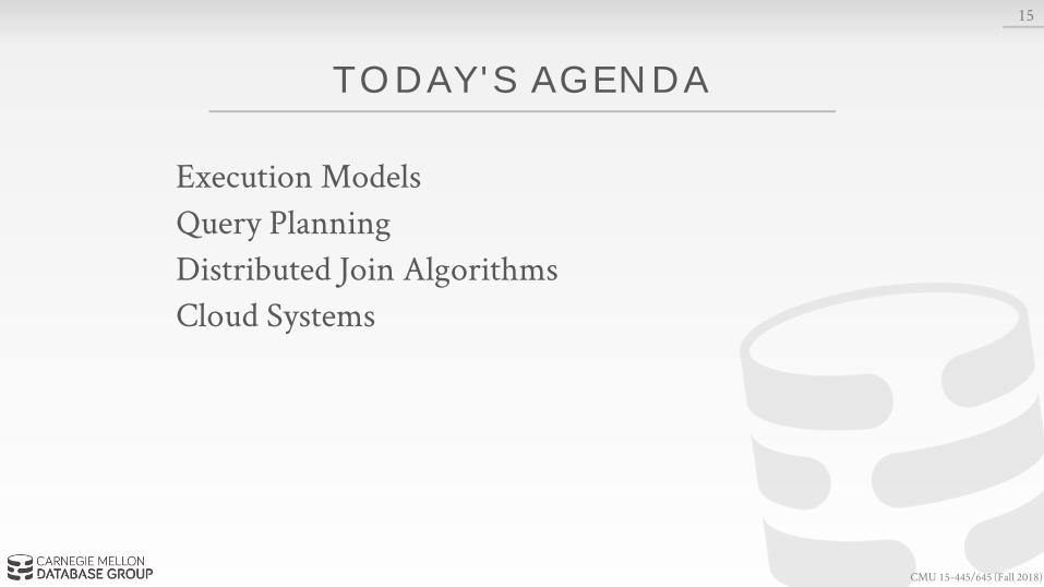
Execution Models
Query Planning
Distributed Join Algorithms
Cloud Systems
15
CMU 15-445/645 (Fall 2018)
PUSH VS. PULL
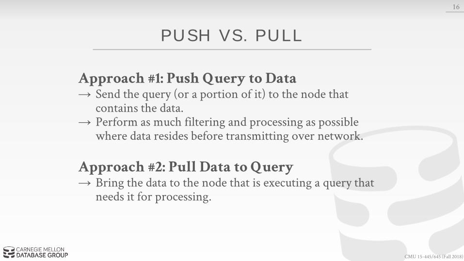
Approach #1: Push Query to Data→ Send the query (or a portion of it) to the node that
contains the data.→ Perform as much filtering and processing as possible
where data resides before transmitting over network.
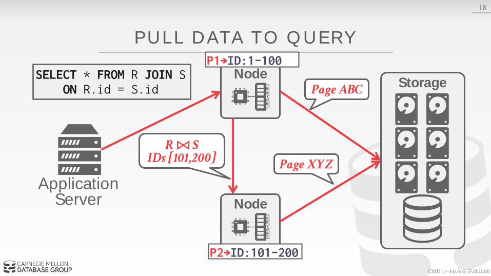
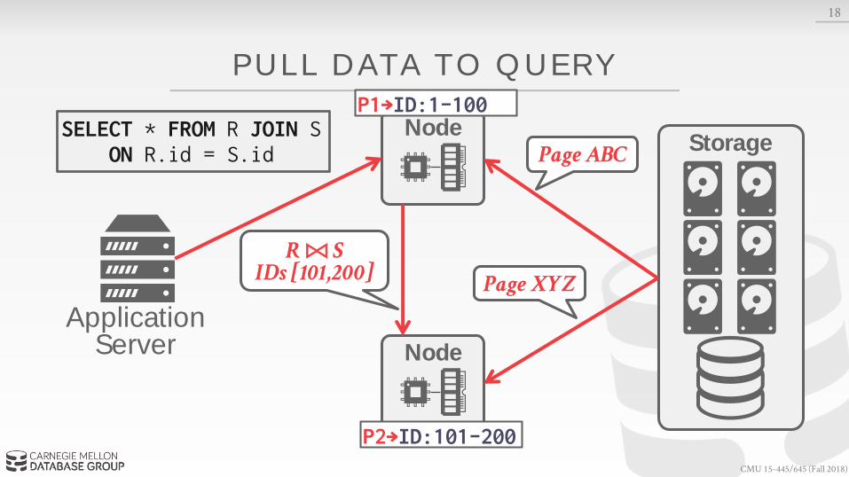
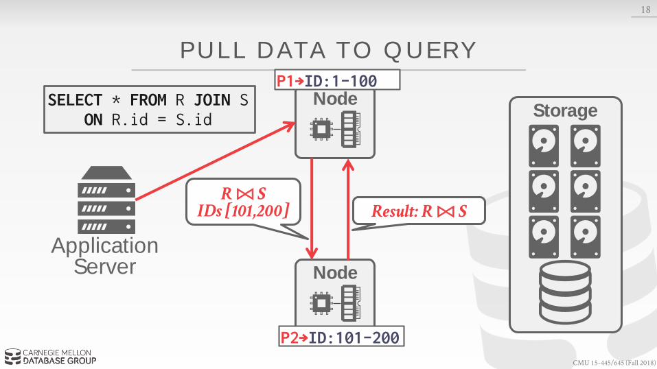
Approach #2: Pull Data to Query→ Bring the data to the node that is executing a query that
needs it for processing.
16

CMU 15-445/645 (Fall 2018)
PUSH QUERY TO DATA
17
Node
ApplicationServer Node
P1→ID:1-100
P2→ID:101-200
SELECT * FROM R JOIN SON R.id = S.id
R ⨝ SIDs [101,200] Result: R ⨝ S
CMU 15-445/645 (Fall 2018)
Storage
PULL DATA TO QUERY
18
Node
ApplicationServer Node
Page ABC
Page XYZ
R ⨝ SIDs [101,200]
P1→ID:1-100
P2→ID:101-200
SELECT * FROM R JOIN SON R.id = S.id
CMU 15-445/645 (Fall 2018)
Storage
PULL DATA TO QUERY
18
Node
ApplicationServer Node
Page ABC
Page XYZ
R ⨝ SIDs [101,200]
P1→ID:1-100
P2→ID:101-200
SELECT * FROM R JOIN SON R.id = S.id
CMU 15-445/645 (Fall 2018)
Storage
PULL DATA TO QUERY
18
Node
ApplicationServer Node
R ⨝ SIDs [101,200]
P1→ID:1-100
P2→ID:101-200
SELECT * FROM R JOIN SON R.id = S.id
Result: R ⨝ S
CMU 15-445/645 (Fall 2018)
FAULT TOLERANCE
Traditional distributed OLAP DBMSs were designed to assume that nodes will not fail during query execution. → If the DBMS fails during query execution, then the whole
query fails.
The DBMS could take a snapshot of the intermediate results for a query during execution to allow it to recover after a crash.
21
CMU 15-445/645 (Fall 2018)
QUERY PL ANNING
All the optimizations that we talked about before are still applicable in a distributed environment.→ Predicate Pushdown→ Early Projections→ Optimal Join Orderings
But now the DBMS must also consider the location of data at each partition when optimizing
22
CMU 15-445/645 (Fall 2018)
QUERY PL AN FRAGMENTS
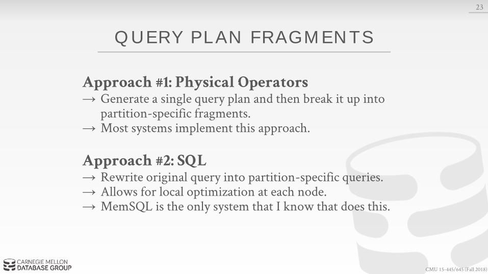
Approach #1: Physical Operators→ Generate a single query plan and then break it up into
partition-specific fragments.→ Most systems implement this approach.
Approach #2: SQL→ Rewrite original query into partition-specific queries.→ Allows for local optimization at each node.→ MemSQL is the only system that I know that does this.
23
CMU 15-445/645 (Fall 2018)
QUERY PL AN FRAGMENTS
25
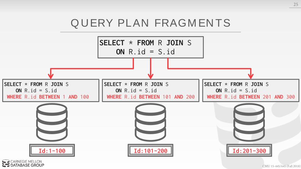
SELECT * FROM R JOIN SON R.id = S.id
Id:1-100
SELECT * FROM R JOIN SON R.id = S.id
WHERE R.id BETWEEN 1 AND 100
Id:101-200
SELECT * FROM R JOIN SON R.id = S.id
WHERE R.id BETWEEN 101 AND 200
Id:201-300
SELECT * FROM R JOIN SON R.id = S.id
WHERE R.id BETWEEN 201 AND 300

CMU 15-445/645 (Fall 2018)
QUERY PL AN FRAGMENTS
25
SELECT * FROM R JOIN SON R.id = S.id
Id:1-100
SELECT * FROM R JOIN SON R.id = S.id
WHERE R.id BETWEEN 1 AND 100
Id:101-200
SELECT * FROM R JOIN SON R.id = S.id
WHERE R.id BETWEEN 101 AND 200
Id:201-300
SELECT * FROM R JOIN SON R.id = S.id
WHERE R.id BETWEEN 201 AND 300
Union the output of each join together to produce final result.
CMU 15-445/645 (Fall 2018)
OBSERVATION
The efficiency of a distributed join depends on the target tables' partitioning schemes.
One approach is to put entire tables on a single node and then perform the join.→ You lose the parallelism of a distributed DBMS.→ Costly data transfer over the network.
26
CMU 15-445/645 (Fall 2018)
DISTRIBUTED JOIN ALGORITHMS
To join tables R and S, the DBMS needs to get the proper tuples on the same node.
Once there, it then executes the same join algorithms that we discussed earlier in the semester.
27
CMU 15-445/645 (Fall 2018)
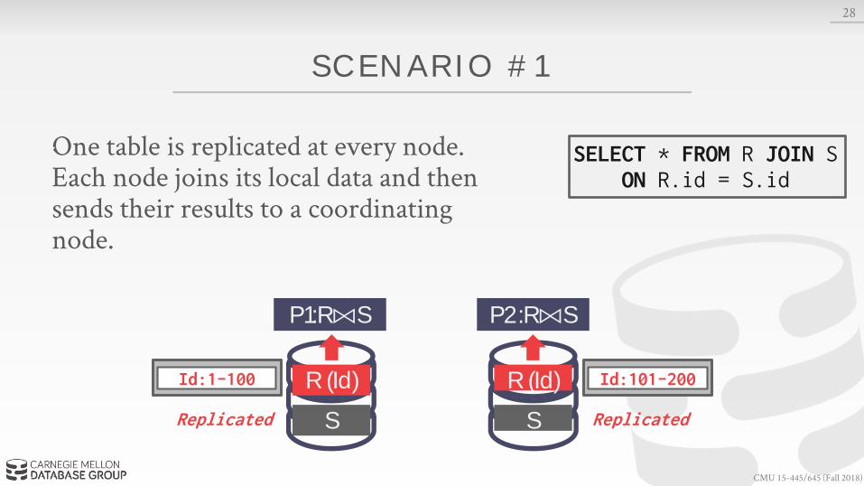
SCENARIO #1
One table is replicated at every node.Each node joins its local data and then sends their results to a coordinating node.
28
R (Id)
S
Id:1-100
Replicated
R (Id)
S
Id:101-200
Replicated
SELECT * FROM R JOIN SON R.id = S.id
P1:R⨝S P2:R⨝S
CMU 15-445/645 (Fall 2018)
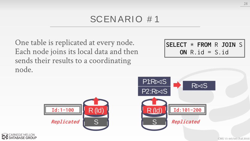
SCENARIO #1
One table is replicated at every node.Each node joins its local data and then sends their results to a coordinating node.
28
R (Id)
S
Id:1-100
Replicated
R (Id)
S
Id:101-200
Replicated
SELECT * FROM R JOIN SON R.id = S.id
P1:R⨝S
P2:R⨝SR⨝S
CMU 15-445/645 (Fall 2018)
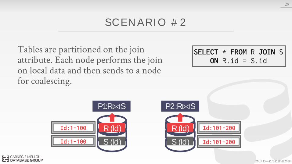
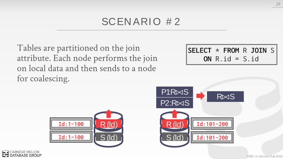
SCENARIO #2
Tables are partitioned on the join attribute. Each node performs the join on local data and then sends to a node for coalescing.
29
R (Id)
S (Id)
Id:1-100 R (Id)
S (Id)
Id:101-200
Id:1-100 Id:101-200
P1:R⨝S P2:R⨝S
SELECT * FROM R JOIN SON R.id = S.id
CMU 15-445/645 (Fall 2018)
SCENARIO #2
Tables are partitioned on the join attribute. Each node performs the join on local data and then sends to a node for coalescing.
29
R (Id)
S (Id)
Id:1-100 R (Id)
S (Id)
Id:101-200
Id:1-100 Id:101-200
P1:R⨝S
P2:R⨝SR⨝S
SELECT * FROM R JOIN SON R.id = S.id

CMU 15-445/645 (Fall 2018)
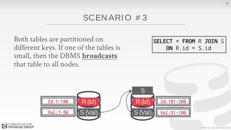
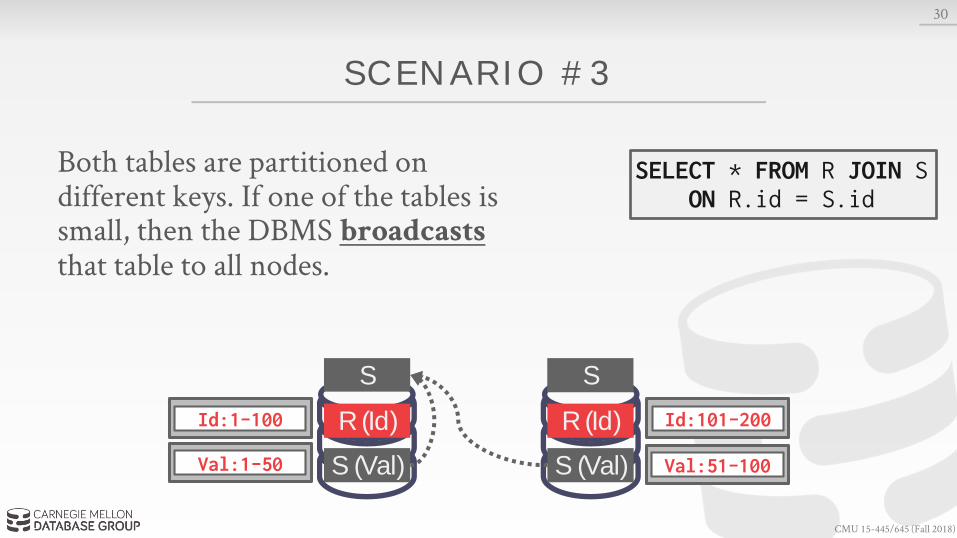
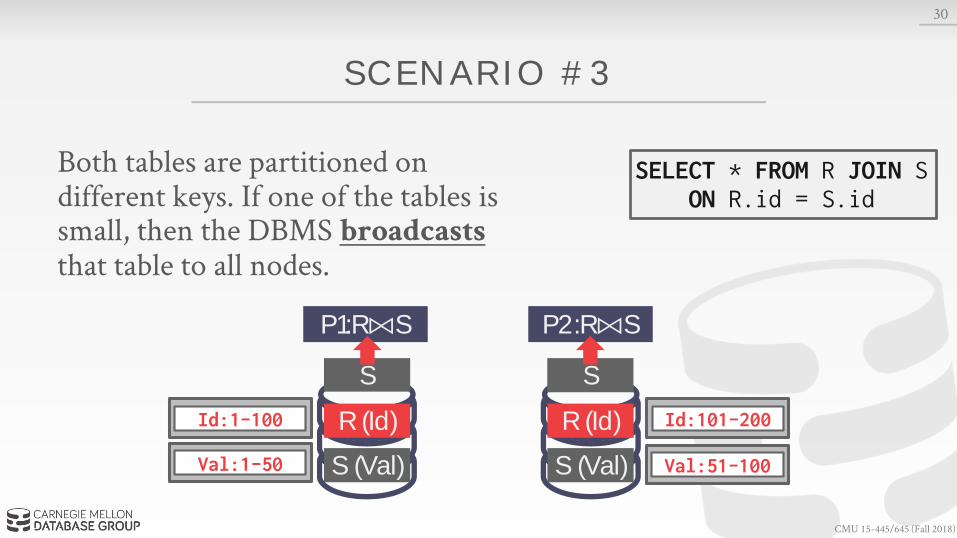
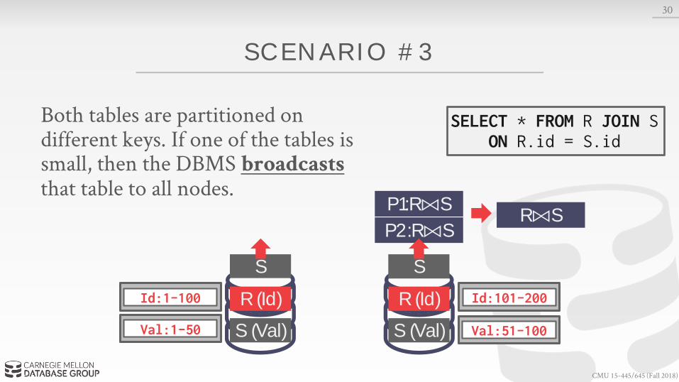
SCENARIO #3
Both tables are partitioned on different keys. If one of the tables is small, then the DBMS broadcaststhat table to all nodes.
30
R (Id)
S (Val)
Id:1-100 R (Id)
S (Val)
Id:101-200
Val:1-50 Val:51-100
SELECT * FROM R JOIN SON R.id = S.id
CMU 15-445/645 (Fall 2018)
SCENARIO #3
Both tables are partitioned on different keys. If one of the tables is small, then the DBMS broadcaststhat table to all nodes.
30
R (Id)
S (Val)
Id:1-100 R (Id)
S (Val)
Id:101-200
Val:1-50 Val:51-100
S
SELECT * FROM R JOIN SON R.id = S.id
CMU 15-445/645 (Fall 2018)
SCENARIO #3
Both tables are partitioned on different keys. If one of the tables is small, then the DBMS broadcaststhat table to all nodes.
30
R (Id)
S (Val)
Id:1-100 R (Id)
S (Val)
Id:101-200
Val:1-50 Val:51-100
S S
SELECT * FROM R JOIN SON R.id = S.id
CMU 15-445/645 (Fall 2018)
SCENARIO #3
Both tables are partitioned on different keys. If one of the tables is small, then the DBMS broadcaststhat table to all nodes.
30
R (Id)
S (Val)
Id:1-100 R (Id)
S (Val)
Id:101-200
Val:1-50 Val:51-100
S S
P1:R⨝S P2:R⨝S
SELECT * FROM R JOIN SON R.id = S.id
CMU 15-445/645 (Fall 2018)
SCENARIO #3
Both tables are partitioned on different keys. If one of the tables is small, then the DBMS broadcaststhat table to all nodes.
30
R (Id)
S (Val)
Id:1-100 R (Id)
S (Val)
Id:101-200
Val:1-50 Val:51-100
S S
P1:R⨝S
P2:R⨝SR⨝S
SELECT * FROM R JOIN SON R.id = S.id
CMU 15-445/645 (Fall 2018)
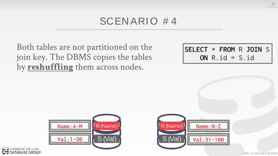
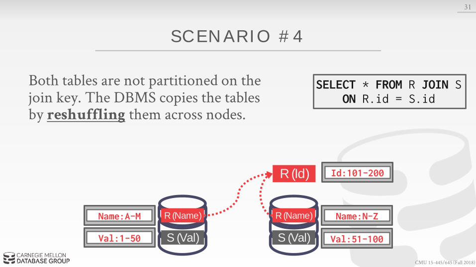
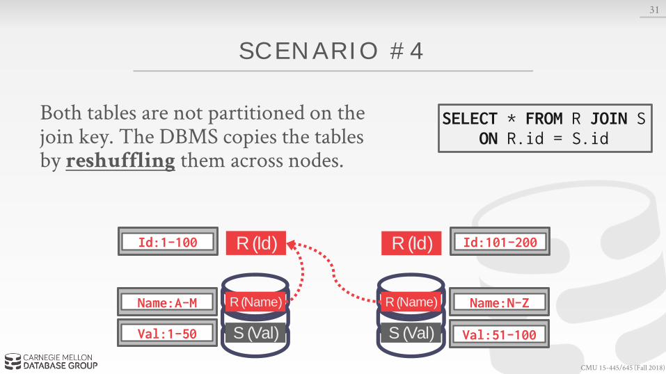
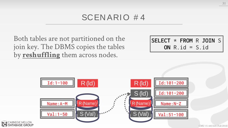
SCENARIO #4
Both tables are not partitioned on the join key. The DBMS copies the tables by reshuffling them across nodes.
31
R (Name)
S (Val)
Name:A-M R (Name)
S (Val)
Name:N-Z
Val:1-50 Val:51-100
SELECT * FROM R JOIN SON R.id = S.id
CMU 15-445/645 (Fall 2018)
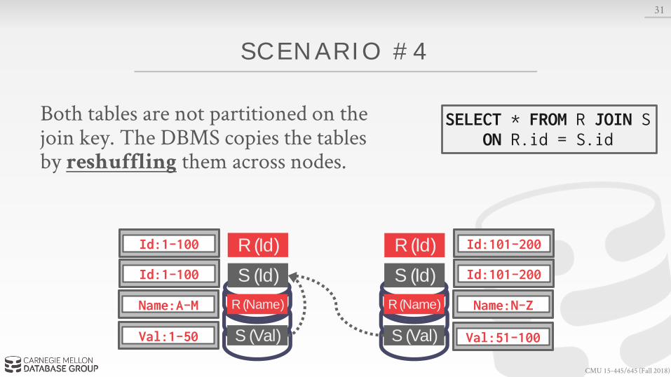
SCENARIO #4
Both tables are not partitioned on the join key. The DBMS copies the tables by reshuffling them across nodes.
31
R (Name)
S (Val)
Name:A-M R (Name)
S (Val)
Name:N-Z
Val:1-50 Val:51-100
R (Id) Id:101-200
SELECT * FROM R JOIN SON R.id = S.id
CMU 15-445/645 (Fall 2018)
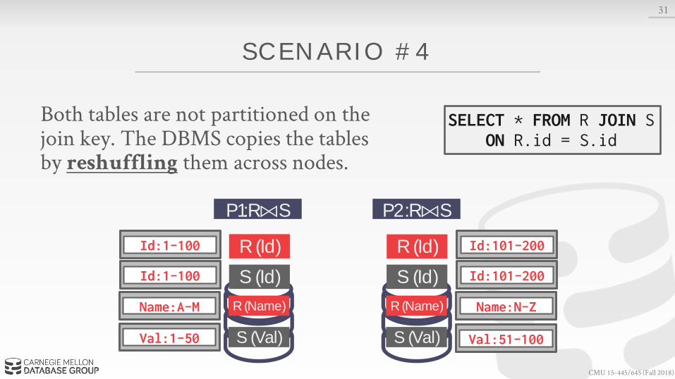
SCENARIO #4
Both tables are not partitioned on the join key. The DBMS copies the tables by reshuffling them across nodes.
31
R (Name)
S (Val)
Name:A-M R (Name)
S (Val)
Name:N-Z
Val:1-50 Val:51-100
R (Id)Id:1-100 R (Id) Id:101-200
SELECT * FROM R JOIN SON R.id = S.id
CMU 15-445/645 (Fall 2018)
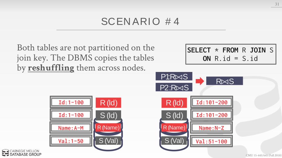
SCENARIO #4
Both tables are not partitioned on the join key. The DBMS copies the tables by reshuffling them across nodes.
31
R (Name)
S (Val)
Name:A-M R (Name)
S (Val)
Name:N-Z
Val:1-50 Val:51-100
Id:101-200S (Id)
R (Id)Id:1-100 R (Id) Id:101-200
SELECT * FROM R JOIN SON R.id = S.id
CMU 15-445/645 (Fall 2018)
SCENARIO #4
Both tables are not partitioned on the join key. The DBMS copies the tables by reshuffling them across nodes.
31
R (Name)
S (Val)
Name:A-M R (Name)
S (Val)
Name:N-Z
Val:1-50 Val:51-100
Id:1-100 S (Id) Id:101-200S (Id)
P1:R⨝S P2:R⨝S
R (Id)Id:1-100 R (Id) Id:101-200
SELECT * FROM R JOIN SON R.id = S.id
CMU 15-445/645 (Fall 2018)
SCENARIO #4
Both tables are not partitioned on the join key. The DBMS copies the tables by reshuffling them across nodes.
31
R (Name)
S (Val)
Name:A-M R (Name)
S (Val)
Name:N-Z
Val:1-50 Val:51-100
Id:1-100 S (Id) Id:101-200S (Id)
P1:R⨝S
P2:R⨝SR⨝S
R (Id)Id:1-100 R (Id) Id:101-200
SELECT * FROM R JOIN SON R.id = S.id
CMU 15-445/645 (Fall 2018)
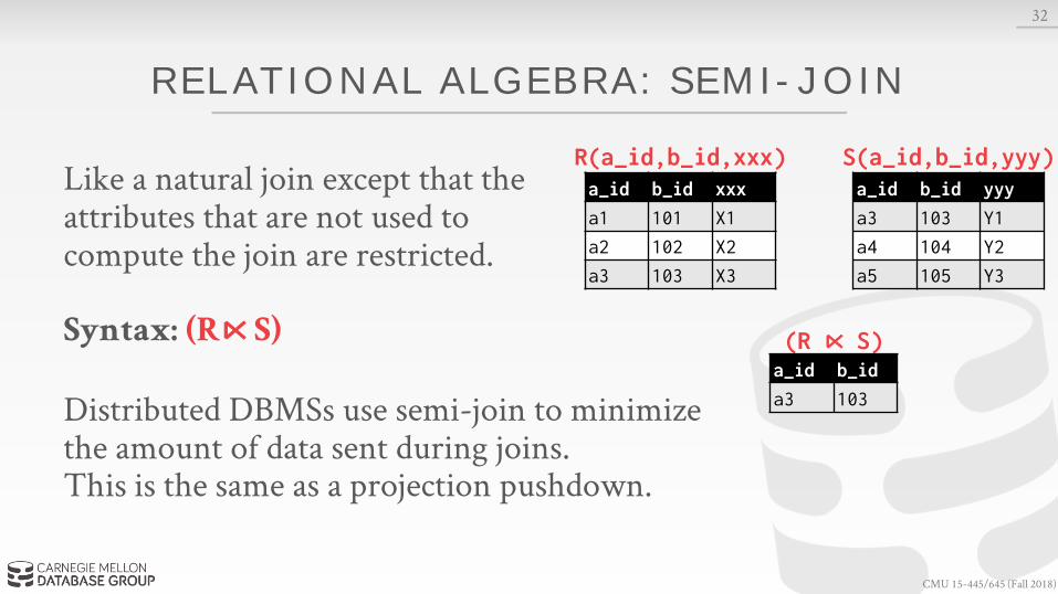
REL ATIONAL ALGEBRA: SEMI-JOIN
Like a natural join except that the attributes that are not used tocompute the join are restricted.
Syntax: (R⋉ S)
32
a_id b_id xxx
a1 101 X1
a2 102 X2
a3 103 X3
R(a_id,b_id,xxx) S(a_id,b_id,yyy)a_id b_id yyy
a3 103 Y1
a4 104 Y2
a5 105 Y3
(R ⋉ S)a_id b_id
a3 103Distributed DBMSs use semi-join to minimize the amount of data sent during joins.This is the same as a projection pushdown.
CMU 15-445/645 (Fall 2018)
CLOUD SYSTEMS
Vendors provide database-as-a-service (DBaaS) offerings that are managed DBMS environments.
Newer systems are starting to blur the lines between shared-nothing and shared-disk.
33

CMU 15-445/645 (Fall 2018)
CLOUD SYSTEMS
Approach #1: Managed DBMSs→ No significant modification to the DBMS to be "aware"
that it is running in a cloud environment.→ Examples: Most vendors
Approach #2: Cloud-Native DBMS→ The system is designed explicitly to run in a cloud
environment. → Usually based on a shared-disk architecture.→ Examples: Snowflake, Google BigQuery, Amazon
Redshift, Microsoft SQL Azure
34
CMU 15-445/645 (Fall 2018)
UNIVERSAL FORMATS
Traditional DBMSs store data in proprietary binary file formats that are incompatible.
One can use text formats (XML/JSON/CSV) to share data across different systems.
There are now standardized file formats.
35

CMU 15-445/645 (Fall 2018)
UNIVERSAL FORMATS
Apache Parquet→ Compressed columnar storage from Cloudera/Twitter
Apache ORC→ Compressed columnar storage from Apache Hive.
HDF5→ Multi-dimensional arrays for scientific workloads.
Apache Arrow→ In-memory compressed columnar storage from Pandas/Dremio
36
CMU 15-445/645 (Fall 2018)
CONCLUSION
Again, efficient distributed OLAP systems are difficult to implement.
More data, more problems…
37
CMU 15-445/645 (Fall 2018)
NEXT CL ASS
VoltDB Guest Speaker
38