Distributed Metric Calibration of Large Camera Networks

Dhanya Devarajan and Richard J. Radke∗

Department of Electrical, Computer, and Systems EngineeringRensselaer Polytechnic Institute, Troy, NY, 12180 USA

devard@rpi.edu,rjradke@ecse.rpi.edu

Abstract

Motivated by applications in surveillance sensor networks,we present a distributed algorithm for the automatic, exter-nal, metric calibration of a network of cameras with nocentralized processor. We model the set of uncalibratedcameras as nodes in a communication network, and pro-pose a distributed algorithm in which each camera onlycommunicates with other cameras that image some of thesame scene points. Each node independently forms aneighborhood cluster on which the local calibration takesplace, and calibrated nodes and scene points are incremen-tally merged into a common coordinate frame. The accu-rate performance of the algorithm is illustrated using ex-amples that model real-world sensor networking situations.

Keywords: camera calibration, metric reconstruction, dis-tributed algorithms, sensor networks, bundle adjustment,structure from motion.

1. Introduction

Existing computer vision research on collections of tensor hundreds of cameras generally takes place in a controlledenvironment with a fixed camera configuration. Traditionalvision tasks such as tracking, 3D visualization, or terrainmapping are typically undertaken in situations where im-ages from all cameras are quickly communicated to a cen-tral processor. In contrast, we are motivated by visionproblems in wireless sensor networks. Such networks willbe essential for 21st century military, environmental, andsurveillance applications [1], but pose many challenges totraditional vision. In a typical scenario, camera nodes arerandomly distributed in an environment and their initial po-sitions are unknown. Even if some nodes are equippedwith GPS receivers, these systems cannot be assumed to

∗This work was supported in part by the US National Science Founda-tion, under the award IIS-0237516.

be highly accurate and reliable [29], and GPS gives no in-formation about the orientation of a directed sensor such asa camera. The nodes are unsupervised after deployment,and generally have no knowledge about the topology of thebroader network [8]. Most nodes are unable to communi-cate beyond a short distance due to power limitations andshort-range antennas, and communication must be kept toa minimum because it is power-intensive.

Furthermore, a realistic camera network is constantly inmotion. The number and location of cameras changes asold cameras wear out and new cameras are deployed to re-place them. Precipitation, wind, and seismic events will joltthe cameras, or remote directives may reposition or reorientthem for a variety of tasks. Mobile cameras mounted in ve-hicles will provide images from time-varying perspectives.Even in a controlled environment like an airport, surveil-lance cameras may be moved randomly to deter terroristswho look for patterns.

This paper is concerned with the problem ofcamera cal-ibration: that is, the estimation of each camera’s 3D posi-tion, orientations, and focal length. Calibration is an essen-tial prerequisite for many computer vision algorithms, suchas multicamera tracking or volume reconstruction. Calibra-tion of a fixed configuration of cameras is an active areaof vision research, and good results are achievable whenthe images are all accessible to a powerful, central proces-sor. On the other hand, here we present adistributedalgo-rithm that can extend todynamicnetworks of cameras. Weview this work as the first step in a new research domain ofdynamic camera networks that incorporates state-of-the-artalgorithms in both computer vision and wireless network-ing.

We model a set of uncalibrated cameras as nodes in acommunication network, and propose a distributed algo-rithm in which each camera only communicates with othercameras that image some of the same scene points. Eachnode independently forms a neighborhood cluster on whichthe local calibration takes place, and calibrated nodes andscene points are incrementally merged into a common co-ordinate frame. The accurate performance of the algorithmis illustrated using examples that model real-world sen-

sor networking situations. Section 2 reviews prior workon multicamera systems and their calibration. Section 3describes our distributed, metric reconstruction algorithm,and Section 4 demonstrates the results of the algorithm forrealistic test data. We conclude in Section 5.

2. Prior Work

This paper concentrates on issues related to computervision, as opposed to explicitly modeling the communi-cation network. We implicitly make several assumptionsbased on active research problems with good preliminarysolutions in the wireless networking community:

1. Nodes that are able to directly communicate can auto-matically determine that they are neighbors. In a realsensor network, these links are formed by radio, in-frared, or optical media [1, 28].

2. If each node knows its one-hop neighbors, a messagefrom one specific node to another can be delivered ef-ficiently (i.e. without broadcasting to the entire net-work) [3, 4, 5, 24].

3. If necessary, a message can be sent efficiently fromone node to all the other nodes [15, 19].

Also, we assume that data communication between nodeshas a much higher cost (e.g. in terms of power consump-tion) than data processing within a node [27], so that mes-sages between nodes should be compact.

In the remainder of this section we discuss prior workrelated to multi-camera calibration. While there has beena substantial amount of work for 1-, 2-, and 3-camerasystems where the cameras share roughly the same pointof view, we are primarily interested in relatively wide-baseline settings where the cameras number in the tens orhundreds and have very different perspectives.

2.1. Multicamera Systems

There are only a few research systems in which tens orhundreds of cameras simultaneously observe a scene, andthese systems are usually housed in a highly controlled lab-oratory environment. Such systems include the VirtualizedReality project at Carnegie Mellon University [17] and sim-ilar stage areas at the University of California at San Diego[23] and the University of Maryland [6]. Such systems aretypically carefully calibrated using test objects of knowngeometry, and an accurate initial estimate of the cameras’positions and orientations.

There are relatively more systems in which a single cam-era acquires many images of a static scene from differentlocations (e.g. [12, 20]), but the cameras in such situa-tions are generally closely spaced. Notable cases in which

many images are acquired from widely spaced positions ofa single camera are include Debevec et al. [7] and Teller etal. [38]. However, in these cases, rough calibration of thecameras was availablea priori, from an explicit model ofthe 3-D scene or from GPS receivers.

From the networking side, various researchers have ex-plored the idea of a Visual Sensor Network (VSN), whereeach node has an image or video sequence that is to beshared/combined/interpreted by other nodes [11, 25, 42,43]. However, most of these discussions have not exploitedthe full potential of the state of the art in computer vision.

2.2. Multicamera Calibration

Typically, a camera is described by two sets of param-eters: internal and external. Internal parameters includethe focal length, position of principal points and the skew.The external parameters describe the placement of the cam-era in a world coordinate system using a rotation matrixand a translation vector. The classical problem of exter-nally calibrating a pair of cameras is well-understood [40];the parameter estimation usually requires a set of featurepoint correspondences in both images. When no pointswith known 3-D locations in the world coordinate frameare available, the cameras can be calibrated up to a sim-ilarity transformation [14]. N -camera calibration can beaccomplished by minimizing a nonlinear cost function ofthe calibration parameters and a collection of unknown 3-Dscene points projecting to matched image correspondences;this process is calledbundle adjustment[39].

Several algorithms have been proposed for calibration ofimage sequences through the estimation of projective trans-formations [18, 30], fundamental matrices [44] or trifocaltensors [10] between nearby images. However, such meth-ods operate only on closely-spaced, explicitly ordered se-quences of images, as might be obtained from a video cam-era, and are designed to obtain a good initial estimate forbundle adjustment to be undertaken at a central processor.Svoboda et al. [36] proposed a multi-camera system wherea person carrying a laser pointer walks around the roomand calibration is obtained by tracking the pointer acrossall images. This is again a centralized calibration problemwhere calibration depends on presence of common scenepoints across all images.

Teller and Antone [37] and Sharp [33] both consideredcalibration of a number of unordered views related by agraph similar to the vision graph we describe in Section 3below. Schaffalitzky and Zisserman [31] recently describedan automatic clustering method for a set of unordered im-ages from different perspectives, which corresponds to con-structing a vision graph containing several complete sub-graphs. We emphasize the main point that sets our workapart from these systems: none of them view the collection

of cameras as the nodes in a communication network, andnone of their algorithms are distributed.

3. Distributed Metric Calibration

We propose to model the sensor network with two undi-rected graphs: acommunication graphand avision graph.We illustrate the idea in Figure 1 with a hypothetical net-work of ten nodes.

A B

C D E F

G H J

K

A B

C D E F

G H J

K

A B

C D E F

G H J

K

(a)

(b) (c)

Communication graph Vision graph

Figure 1. (a) A snapshot of the instantaneous state ofa camera network, indicating the fields of view of tencameras. (b) The associated communication graph.(c) The associated vision graph. Note the presenceof an edge in one graph does not imply the presenceof the same edge in the other graph.

Figure 1a shows a snapshot of the locations and orien-tations of the cameras. Figure 1b illustrates the communi-cation graph for the network; an edge appears between twocameras in this graph if they have one-hop direct commu-nication. This is a common abstraction in wireless ad-hocnetworks (see [13] for a review). The communication graphis mostly determined by the locations of the nodes and thetopography of the environment; in a wireless setting, theinstantaneous power each node can expend towards com-munication is also a factor.

Figure 1c illustrates thevision graphfor the network;an edge appears between two cameras in this graph if they

observe some of the same scene points from different per-spectives. We note that the presence of an edge in the com-munication graph does not imply the presence of the sameedge in the vision graph, since the cameras may be pointedin different directions (for example, camerasA and C).Conversely, an edge can connect two cameras in the visiongraph despite a lack of physical proximity between them(for example, camerasC andF ). In networking terminol-ogy, the vision graph is a called anoverlay graphon thecommunication network.

Ideally, the vision graph should be estimated automati-cally, rather than constructed manually [33] or specifiedapriori [37]. However, for the purposes of this initial investi-gation, we assume that the feature correspondences used inthe calibration procedure are given. We note that establish-ing robust feature correspondences across many images isitself a difficult problem, even in the centralized case. In thefuture, we plan to automatically establish arcs in the visiongraph by detecting and matching invariant features [21, 22].Furthermore, while we consider the static case here, visionand communication graphs in real sensor-networking ap-plications will be dynamic due to the changing presence,position and orientation of each camera in the network, aswell as time-varying channel conditions.

Our goal is to design a calibration system in which eachcamera only communicates with (and possesses knowledgeabout) those cameras connected to it by an edge in the vi-sion graph. We assume that each camera node calibratesindependently of the rest by estimating a metric reconstruc-tion based on a local cluster formed by neighboring cam-eras in the vision graph. We refer to the calibration at anode as thelocal calibration. Arbitrary coordinate framesarising from local calibrations are then aligned iterativelyto a common Coordinate frame. The following sectionsdescribe the details of each of these phases.

3.1. Notation

We assume that the vision graph containsM nodes, eachrepresenting a perspective camera described by a 3x4 ma-trix Pi:

Pi = Ki [Ri, ti] . (1)

Here,Ri ∈ SO(3) andti ∈ R3 are the rotation matrix andtranslation vector comprising the external camera parame-ters. Ki is the intrinsic parameter matrix and is assumedhere to bediag(fi, fi, 1), wherefi is the focal length.1

Each camera images some subset of a set ofN pointsX ∈ R3. This subset is described byVi ⊂ 1, . . . , N.

1Aspect ratio, center of projection and image skew can be easily in-corporated into theK matrix and the following algorithm. Lens distortionmay also be a factor in real camera networks, but this distortion does notneed to be estimated with reference to other cameras.

u11 u22

X1

u12 u21

f1 f2

X2

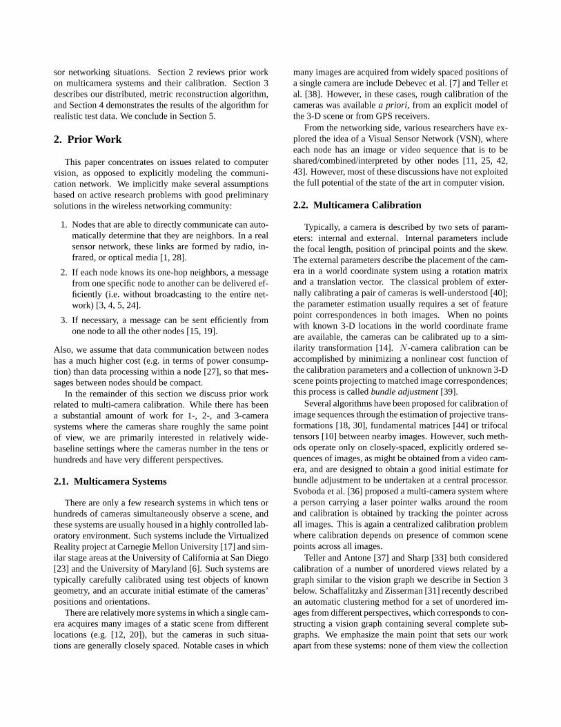
P1 P2

Figure 2. Notation and geometry of the imaging sys-tem.

The projection ofXj onto Pi is given byuij ∈ R2 forj ∈ Vi:

λij

[uij

1

]= Pi

[Xj

1

], (2)

whereλij is called the projective depth [35]. This imageformation process is illustrated in Figure 2. The simplifiedK matrix assumption for the camera is just to provide anexample model for the scheme. The mathematics of thetechnique does accommodate for more generalized models(see below).

Edges are culled from the vision graph based on neigh-borhood sufficiency conditions (i.e. there must be a mini-mal number of neighbors per node that must jointly imagesome minimal number of points). We define a characteris-tic functionχij whereχij = 1 if nodej satisfies the suffi-ciency conditions at nodei. Thus each node is associatedwith a cluster,Ci, on which the local calibration is carriedout:

Ci = j | χij = 1

In our experiments, we chose a minimum cluster size of4 nodes that must share 12 corresponding points. At eachnodei, the local calibration results in an estimate of thelocal camera parametersP i

i as well as the camera param-eters ofi’s neighbors,P i

j , j ∈ Ci. (Conversely, thismeans that each of camerai’s neighbors will have a slightlydifferent estimate of wherei is; we discuss how to rec-oncile these differences below.) The 3D scene points re-constructed ati are given byXi

k, which are estimates ofXk|k ∈

⋂j∈i,Ci Vj. If neighborhood sufficiency con-

ditions are not met at a node, then local calibration doesnot take place (though an estimate can still be obtained; seebelow).

3.2. Local Calibration

Here, we describe the local calibration problem at nodei. We denoteP1, . . . , Pm as the cameras ini’s cluster,wherem = |i, Ci|. Similarly, we denoteX1, . . . , Xnas the 3D points used for calibration, wheren = |Xk|k ∈⋂

j∈i,Ci Vj|. Nodei must estimate the camera parame-tersP as well as the unknown scene pointsX using onlythe 2D image correspondencesuij , i = 1, . . . ,m, j =1, . . . , n.

Taking into account all the image projections, (2) can bewritten as

W =

λ11u11 λ12u12 . . . λ1nu1n

λ21u21 λ22u22 . . . λ2nu2n

...λn1un1 λn2un2 . . . λnnunn

=

P1

P2

...Pm

(Xh

1 Xh2 . . . Xh

n

).

(3)Here,Xh denotesX represented in homogeneous coordi-nates, i.e.Xh = [XT , 1]T .

Sturm and Triggs [35] suggested a factorization methodthat recovers the projective depths as well as the structureand motion parameters from the above equation. They usedrelationships between fundamental matrices and epipolarlines in order to recover the projective depthsλij . Oncethe projective depths are recovered, the structure and mo-tion are recovered by SVD factorization of the best rank-4approximation to the measurement matrixW :

W = U3m×4ΣV4×n

=(U3m×4

√Σ

) (√ΣV4×n

)

=

P1

P2

...Pm

3m×4

(Xh

1 Xh2 . . . Xh

n

)4×n

.

However, there is a projective ambiguity in the reconstruc-tion, since (

PH−1) (

HX)

= P X. (4)

for any 4 × 4 nonsingular matrixH. There exists someHi relating the projective factorization to the true metric(i.e. Euclidean) factorization, given by

PiH−1i = Ki

[Ri ti

]. (5)

This Hi can be estimated by using the dual to absoluteconic, which remains invariant under rigid transformations

[14]. The dual to the absolute conic,Ω, satisfies the equa-tion

PiΩPTi ∝ KiK

Ti = αiωi. (6)

whereωi is the dual to the image of the absolute conic andαi is the constant of proportionality. The homographyHi

satisfiesΩ = HHT . (7)

whereH is the first 3 columns ofHi. Seo, Heyden andCipolla [32] and Pollefeys [26] proposed methods for trans-forming a projective factorization into a metric one basedon (6)-(7). The Euclidean reconstruction so recovered is re-lated to the true camera/scene configuration by an unknownsimilarity transform that cannot be estimated without addi-tional measurements of the scene. As mentioned before theabove schemes also accommodate more generalized cam-era models.

The above scheme might fail under two conditions.First, there may be a small fraction of outliers in the cor-respondences, e.g. caused by repetitive patterns in the im-ages, that can cause the parameter estimates to be inaccu-rate. Standard rejection algorithms such as RANSAC [9]should be able to detect and remove such outliers. It is alsopossible that the camera cluster might be close to a criticalconfiguration of the metric reconstruction and might resultin a poorly conditioned problem. For example, cameraswhose centers are collinear or that have a common centerof focus are critical for metric calibration [34]. Hence, thelocal calibration procedure may yield unreliable estimates.Such failures typically can be detected automatically fromlarge reprojection errors or disproportionately large valuesof the estimated internal parameters. However, the failureof calibration at a particular node can be easily compen-sated for by obtaining one of the neighboring estimates,e.g. nodei can calibrate its camera based on nodej’s esti-mation,P j

i , j ∈ Ci.

3.3. Frame Alignment

The estimates obtained by local calibrations have differ-ent coordinate frames, each offset from the true frame byan unknown similarity transformation (i.e. rotation, trans-lation, and scaling). In order for cameras on the networkto coordinate higher-level vision tasks, we require a dis-tributed algorithm to align all nodes to a common coordi-nate frame.

We assume each node has a unique identifieridi ∈ R,such as a factory serial number, and an alignment indexai that is initially set toidi. Each nodei then continuallyaligns its frame to theavailableneighbor with lowest align-ment indexaj , j ∈ Ci. By “available”, we mean a neighbornode that is not currently aligning its frame to that of nodei. Ultimately, if the vision graph is connected, each frame

will be aligned to the frame of the camera with the lowestidentifier; a similar scheme was presented and analyzed in[16]. The procedure at nodei is as follows.

1. Letjmin = arg minj∈Ciaj , andamin = ajmin .

2. If amin < ai, then

(a) Align nodei to the frame of nodejmin.

(b) Setai = amin.

3. Iterate.

The alignment process in step 2a is accomplished by solv-ing

minS

∑k∈Vi∩Vjmin

‖SXik − Xjmin

k ‖2,

whereS is constrained to be a similarity transform. Thisminimization can be accomplished in closed form byUmeyama’s method [41]. After convergence, there maystill be some disagreement betweenXi

k and Xjk, j ∈ Ci,

which we deal with by averaging all local estimates for agiven pointXk in the common coordinate frame. We notethat this step is not strictly necessary when the main goal isto calibrate the cameras, not to recover the structure.

An interesting question is how to determine, in a dis-tributed manner, the node that requires the fewest numberof alignment transformations (thus minimizing error ac-cumulation). This node (i.e. the barycenter of the visiongraph) could be assigned to have the lowest identifier in theabove scheme.

3.4. Summary

The entire algorithm for distributed calibration is sum-marized below:

1. Form the vision graph from the set of correspondencescontained inM views.

2. At each nodei,

(a) Form a subnetCi with at least 12 common imagemeasurement points and 4 nodes.

(b) Estimate a projective reconstruction on the nor-malized points [35].

3. Calculate the residual reprojection errors. If they arelarge, discard the local calibration process. Otherwise,

(a) Form the equation matrix for metric reconstruc-tion and normalize the rows to have unit norm.

(b) Estimate a metric reconstruction based on theprojective cameras [32].

4. Estimate the focal lengths and also the error inthe principal points (we assume principal points areknown). If the error is large or if the estimated fo-cal lengths seem unreasonable, then discard the localcalibration process.

5. Incrementally align each node to a common frame.

(a) Determine the lowest-labeled available neigh-bor.

(b) Estimate a similarity transformation to align theframes [41].

(c) Perform multiple iterations of alignment untilall nodes are initialized and there are no furtherchanges to the frame alignment.

(d) Average all local estimates of the same scenepoint to ensure all nodes share the same esti-mated structure, if desired.

4. Experiments

We studied the algorithm’s performance for simulateddata by comparing the structure and calibration parametersestimated using the distributed algorithm to ground truth.Both datasets are aligned to the same similarity frame be-fore comparison. The structural error (i.e. error inX ’s) iscalculated as the average distance between the the groundtruth and the reconstructed points, relative to the scene di-ameter. Calibration errors are described by orientation, fo-cal length, and camera center errors. Orientation error ismeasured in terms of the angle between corresponding op-tical axes, and focal length error as the deviation from unityof the ratio of the true and estimated values. Error in thecamera center is calculated as the average distance betweenthe the ground truth and the estimated centers, relative tothe scene diameter.

The following section discusses the details of two exper-iments: one with many realizations of random scene pointsand image noise, and one with a more realistic model ofcamera/scene placement with occlusions.

4.1. Experiment 1

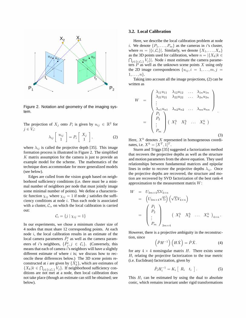
500 scene points were uniformly (randomly) distributedin a 5m-radius sphere and 40 camera nodes (focal length5cm, zero skew and principal points on image center)were positioned randomly on an elliptical band around thesphere. Each camera was oriented to view a random lo-cation inside the scene. Due to limited field of view, eachcamera images only a portion of the scene (see Figure 3).The local calibration cluster at each camera consists ofyet fewer scene points due to the neighborhood sufficiencyconditions.

0 5 10 15 20 25 30 35 400

10

20

30

40

50

60

Node id

% o

f sc

ene

poin

ts

% of scene points in cluster at a node% of scene points imaged at a node

Figure 3. A typical example of the percentage ofscene points imaged at each camera (dashed line)and the percentage of scene points in each local cali-bration cluster (solid line).

Scene points were projected to image planes, and thenperturbed with Gaussian noise of standard deviation of 0.5,1, 1.5, 2 and 2.5 pixels. For each node, the median re-construction error was calculated. The experiment was re-peated with 10 different scene configurations and 10 dif-ferent perturbations for each noise level. The median re-construction errors were then averaged over these multiplerealizations of noise and scene configurations. Quantitativeanalysis of the calibration procedure is summarized in Ta-ble 1, including the reconstruction error in the 3D points,the Mahalanobis reprojection errors, and camera position,orientation, and focal length errors (recovered from the de-composition (1)).

The overall reconstruction accuracy of scene points isquite good, even in the presence of noise: less than 0.7%median relative error. The Mahalanobis reprojection error,defined as

‖u− u‖ =((u− u)T Σ−1(u− u)

)1/2

whereΣ is the covariance of the image pixels, is also low(< 5), indicating reasonably good estimates.

While the camera orientation error is small, less than0.14 radians, the relative positional error in the cameracenters are quite large for larger values of noise variance(e.g. 9% in the worst case). This indicates that the origi-nal and recovered optical axes are nearly parallel, but thatthe reconstructed cameras are mis-positioned. We note thatthis sensitivity in camera center estimation is an expectedphenomenon and not a failure of the algorithm; moving acamera along its optical axis has a relatively small effect

Noise Xerr Cerr ferr Angerr Reprojection errorvariance Mahalanobis Euclidean0 0 0 0 0 0 00.5 0.0897 1.4027 0.0023 0.0261 3.5760 1.78801 0.1993 3.1593 0.0059 0.0527 3.7597 3.75971.5 0.3370 4.7759 0.0070 0.0789 3.4578 5.18682 0.5109 6.1991 0.0133 0.1120 3.5863 7.17262.5 0.6710 9.0693 0.0215 0.1324 4.9618 12.4046

Table 1. Error Table : Xerr : Distance errors in scene recovery (percentage of scene width); Cerr : Errors incamera centers (percentage of scene width); ferr: Focal length error expressed as a relative fraction; Angerr:Orientation error expressed as angular difference between the optical axes (in rad); Reprojection error : Errordistance between the original image and the reprojected image points : Mahalanobis distance (dimensionless)and Euclidean distance (in pixels)

on the position of projected points in the absence of severeperspective effects. Indeed, this error in camera centers haslittle influence on the structure estimation or on the repro-jection error that is the basis for the local calibrations.

As for the internal camera parameters, focal lengths areestimated quite accurately (less than 0.03% error). Herewe have assumed known principal points. If the estimatedprincipal point of the local calibration at nodei is far fromthe known value, the local estimate is rejected and an esti-mate obtained from one of nodei’s neighbors.

Only a portion of the 3D points jointly imaged by all thecameras are reconstructed, due to the neighborhood suffi-ciency constraints. However, after all nodes have been cal-ibrated, it is straightforward to estimate the missing scenepoints via a triangulation procedure [2]. Alternately, it isstraightforward to include the scene points imaged by atleast 2 cluster cameras directly in the optimization functionfor bundle adjustment.

4.2. Experiment 2

We also studied the performance of the algorithm withdata modeling a real-world situation with reasonable di-mensions. The scene consisted of 20 cameras survey-ing two simulated (opaque) structures. The cameras wereplaced randomly on an elliptical band around the “build-ings’”. The configuration of the setup is shown in Figure4. Since the image plane is finite and the “buildings” areopaque, each camera sees only about 25% of the scenepoints. A total of 4000 scene points uniformly distributedalong the walls of the buildings were captured by the 20cameras and the imaged points were then perturbed byGaussian random noise with a standard deviation of 1 pixel.

Figures 5a and 5b show the ground-truth configurationand the recovered configuration, respectively. The qualityof the shape recovery is evident. Most of the cameras are

Figure 4. The field of view of each of the simulatedcameras.

well-recovered; the average orientation error is 0.008 radi-ans, while the relative focal length error is 0.015. The meanerror in estimation of camera positions, relative to the scenewidth, is 2.1%, while the median error is 0.7%. Two cam-eras (marked by circles in Figure 5b) are not calibrated dueto failing the neighborhood sufficiency constraints, whileanother camera is particularly poorly calibrated (marked bya square in Figure 5b). We emphasize that the only dataused to obtain this result were the positions of matchingpoints in the images taken by the cameras.

5. Conclusions

We have demonstrated a distributed metric calibrationalgorithm whose results are comparable to centralized al-gorithms. Furthermore, the algorithm is asynchronous in

(a)

(b)

Figure 5. (a) Ground truth structure and camera positions (b) Recovered structure and camera positions. Thetwo circles indicate cameras that are not calibrated and the square indicates a camera that is particularly poorlycalibrated.

the sense that more than one node can process at a time,and there need be no ordering on the node processing.

Since the emphasis on this paper is on demonstratingthe workability of the distributed calibration scheme, wehave assumed ideal networking conditions. While such as-sumptions do simplify the simulations, they do not changethe overall approach in more complicated cases. Analysisof the associated communication issues under varying con-ditions and topologies (e.g. using a network simulator) is

the next logical step towards developing a more realisticmodel of the distributed network. Eventually, we plan tobuild wireless camera nodes to test the performance of ouralgorithms in real situations.

As mentioned above, we plan to generate the visiongraph automatically based on invariant feature matching.We are currently working to develop more principled ver-sions of the frame alignment process based on the underly-ing probability densities of the estimated camera parame-

ters.Finally, we note that distributed camera calibration is

only the first step towards additional distributed computervision algorithms, such as view synthesis or image-basedquery and routing.

References

[1] I. Akyildiz, W. Su, Y. Sankarasubramaniam, and E. Cayirci.Wireless sensor networks: a survey.Computer Networks,38:393–422, 2002.

[2] M. Anderson and D. Betsis. Point reconstruction from noisyimages.Journal of Mathematical Imaging and Vision, 5:77–90, 1995.

[3] L. Blazevic, L. Buttyan, S. Capkun, S. Giordano, J. Hubaux,and J. L. Boudec. Self-organization in mobile ad-hoc net-works: the approach of terminodes.IEEE CommunicationsMagazine., June 2001.

[4] S. Capkun, M. Hamdi, and J. P. Hubaux. GPS-free posi-tioning in mobile ad-hoc networks. In34th HICSS, January2001.

[5] M. Chu, H. Haussecker, and F. Zhao. Scalable information-driven sensor querying and routing for ad hoc heterogeneoussensor networks.Int’l J. High Performance Computing Ap-plications, 2002. Also Xerox Palo Alto Research CenterTechnical Report P2001-10113, May 2001.

[6] L. Davis, E. Borovikov, R. Cutler, D. Harwood, and T. Hor-prasert. Multi-perspective analysis of human action. InPro-ceedings of Third International Workshop on CooperativeDistributed Vision, November 1999. Kyoto, Japan.

[7] P. E. Debevec, G. Borshukov, and Y. Yu. Efficient view-dependent image-based rendering with projective texture-mapping. In9th Eurographics Rendering Workshop, June1998. Vienna, Austria.

[8] D. Estrin et al.Embedded, Everywhere: A Research Agendafor Networked Systems of Embedded Computers. NationalAcademy Press, 2001. Washington, D.C.

[9] M. A. Fischler and R. C. Bolles. Random sample consen-sus: A paradigm for model fitting with applications to imageanalysis and automated cartography.Comm. of the ACM,24:381–395, 1981.

[10] A. W. Fitzgibbon and A. Zisserman. Automatic camera re-covery for closed or open image sequences. InECCV (1),pages 311–326, 1998.

[11] A. E. Gamal. Collaborative visual sensors, 2004.http://mediax.stanford.edu/projects/cvsn.html .

[12] S. Gortler, R. Grzeszczuk, R. Szeliski, and M. Cohen. Thelumigraph. InComputer Graphics (SIGGRAPH ’96), pages43–54, August 1996.

[13] Z. Haas et al. Wireless ad hoc networks. In J. Proakis, editor,Encyclopedia of Telecommunications. John Wiley, 2002.

[14] R. Hartley and A. Zisserman.Multiple View Geometry inComputer Vision. Cambridge University Press, 2000.

[15] J. Hromkovic, R. Klasing, B. Monien, and R. Peine.Dissemination of information in interconnection networks(broadcasting and gossiping). In F. Hsu and D.-A. Du,editors, Combinatorial Network Theory, pages 125–212.

Kluwer, 1995.[16] R. Iyengar and B. Sikdar. Scalable and distributed gps free

positioning for sensor networks. InIEEE ICC, May 2003.[17] T. Kanade, P. Rander, and P. J. Narayanan. Virtualized re-

ality: Constructing virtual worlds from real scenes.IEEEMultimedia, 4(1):34–47, 1997.

[18] E.-Y. Kang, I. Cohen, and G. Medioni. A graph-based globalregistration for 2D mosaics. In15th International Con-ference on Pattern Recognition(ICPR), 2000. Barcelona,Spain.

[19] D. W. Krumme, G. Cybenko, and K. N. Venkataraman. Gos-siping in minimal time. SIAM J. Comput., 21(1):111–139,1992.

[20] M. Levoy and P. Hanrahan. Light field rendering. InComputer Graphics (SIGGRAPH ’96), pages 31–42, August1996.

[21] D. G. Lowe. Object recognition from local scale-invariantfeatures. InInternational Conference on Computer Vision,pages 1150–1157, September 1999.

[22] K. Mikolajczyk and C. Schmid. An affine invariant inter-est point detector. InEuropean Conference on ComputerVision, volume 1, pages 128–142, 2002.

[23] S. Moezzi, L.-C. Tai, and P. Gerard. Virtual view generationfor 3D digital video. IEEE Multimedia, 4(1):18–26, Jan.-March 1997.

[24] D. Niculescu and B. Nath. Trajectory based forwardingand its applications. Technical report, Rutgers University,2002. http://www.cs.rutgers.edu/dataman/papers/tbftr.pdf .

[25] K. Obraczka, R. Manduchi, and J. Garcia-Luna-Aceves.Managing the information flow in visual sensor networks.In The Fifth International Symposium on Wireless PersonalMultimedia Communication (WMPC), October 2002.

[26] M. Pollefeys, R. Koch, and L. J. V. Gool. Self-calibrationand metric reconstruction in spite of varying and unknowninternal camera parameters. InICCV, pages 90–95, 1998.

[27] J. Pottie and W. Kaiser. Wireless integrated network sensors.Communications of the ACM, 3(5):51–58, May 2000.

[28] N. B. Priyantha, A. Chakraborty, and H. Balakrishnan. TheCricket location-support system. InSixth Annual ACM In-ternational Conference on Mobile Computing and Network-ing (MOBICOM), August 2000.

[29] A. Savvides, C. C. Han, and M. B. Srivastava. Dynamicfine-grained localization in ad-hoc wireless sensor networks.In International Conference on Mobile Computing and Net-working (MobiCom) 2001, July 2001.

[30] H. S. Sawhney, S. Hsu, and R. Kumar. Robust video mo-saicing through topology inference and local to global align-ment. InEuropean Conference on Computer Vision, pages103–119, 1998.

[31] F. Schaffalitzky and A. Zisserman. Multi-view matching forunordered image sets, or “How do I organize my holidaysnaps?”. InEuropean Conference on Computer Vision, vol-ume LNCS 2350, pages 414–431, June 2002. Copenhagen,Denmark.

[32] Y. Seo, A. Heyden, and R. Cipolla. A linear iterative methodfor auto-calibration using dac equation. InCVPR, 2001.

[33] G. Sharp, S. Lee, and D. Wehe. Multiview registration of 3-

D scenes by minimizing error between coordinate frames. InEuropean Conference on Computer Vision, volume LNCS2351, pages 587–597, June 2002. Copenhagen, Denmark.

[34] P. Sturm. Critical motion sequences for monocular self-calibration and uncalibrated euclidean reconstruction. InProceedings of the Conference on Computer Vision and Pat-tern Recognition, Puerto Rico, USA, pages 1100–1105, June1997.

[35] P. Sturm and B. Triggs. A factorization based algorithm formulti-image projective structure and motion. InECCV (2),pages 709–720, 1996.

[36] T. Svoboda, H. Hug, and L. V. Gool. Viroom – low costsynchronized multicamera system and its self-calibration. InLNCS 2449, pages 515–522. Springer, 2002.

[37] S. Teller and M. Antone. Scalable, extrinsic calibrationof omni-directional image networks.International Journalof Computer Vision, 49(2/3):143–174, September/October2002.

[38] S. Teller, M. Antone, Z. Bodnar, M. Bosse, S. Coorg,M. Jethwa, and N. Master. Calibrated, registered imagesof an extended urban area. InIEEE CVPR, December 2001.

[39] B. Triggs, P. McLauchlan, R. Hartley, and A. Fitzgibbon.Bundle adjustment – A modern synthesis. In W. Triggs,A. Zisserman, and R. Szeliski, editors,Vision Algorithms:

Theory and Practice, LNCS, pages 298–375. Springer Ver-lag, 2000.

[40] R. Tsai. A versatile camera calibration technique for high-accuracy 3-D machine vision metrology using off-the-shelfTV cameras and lenses. In L. Wolff, S. Shafer, andG. Healey, editors,Radiometry – (Physics-Based Vision).Jones and Bartlett, 1992.

[41] S. Umeyama. Least-squares estimation of transformationparameters between two point patterns.IEEE Transactionson Pattern Analysis and Machine Intelligence, 13(4):376–380, 1991.

[42] H. Wu and A. Abouzeid. Energy efficient distributedJPEG2000 image compression in multihop wireless net-works. In Proceedings of 4th Workshop on Applicationsand Services in Wireless Networks, Boston, Massachusetts,2004.

[43] H. Wu and A. Abouzeid. Power aware image transmissionin energy constrained wireless networks. InProceedings ofThe 9th IEEE Symposium on Computers and Communica-tions (ISCC’2004), Alexandria, Egypt, June 2004., 2004.

[44] Z. Zhang and Y. Shan. Incremental motion estimationthrough local bundle adjustment. Technical report, MSR-TR-01-54, 2001.