June 2003 • NREL/SR-560-34216

T. Regan and H. Sinnock Orion Engineering Corp. Westford, Massachusetts A. Davis University of Massachusetts Lowell Lowell, Massachusetts

Distributed Energy Neural Network Integration System Year One Final Report

National Renewable Energy Laboratory 1617 Cole Boulevard Golden, Colorado 80401-3393 NREL is a U.S. Department of Energy Laboratory Operated by Midwest Research Institute • Battelle • Bechtel

Contract No. DE-AC36-99-GO10337

June 2003 • NREL/SR-560-34216

Distributed Energy Neural Network Integration System Year One Final Report

T. Regan and H. Sinnock Orion Engineering Corp. Westford, Massachusetts A. Davis University of Massachusetts Lowell Lowell, Massachusetts

NREL Technical Monitor: H. Thomas Prepared under Subcontract No. AAD-0-30605-07

National Renewable Energy Laboratory 1617 Cole Boulevard Golden, Colorado 80401-3393 NREL is a U.S. Department of Energy Laboratory Operated by Midwest Research Institute • Battelle • Bechtel

Contract No. DE-AC36-99-GO10337

NOTICE This report was prepared as an account of work sponsored by an agency of the United States government. Neither the United States government nor any agency thereof, nor any of their employees, makes any warranty, express or implied, or assumes any legal liability or responsibility for the accuracy, completeness, or usefulness of any information, apparatus, product, or process disclosed, or represents that its use would not infringe privately owned rights. Reference herein to any specific commercial product, process, or service by trade name, trademark, manufacturer, or otherwise does not necessarily constitute or imply its endorsement, recommendation, or favoring by the United States government or any agency thereof. The views and opinions of authors expressed herein do not necessarily state or reflect those of the United States government or any agency thereof.

Available electronically at http://www.osti.gov/bridge

Available for a processing fee to U.S. Department of Energy and its contractors, in paper, from:

U.S. Department of Energy Office of Scientific and Technical Information P.O. Box 62 Oak Ridge, TN 37831-0062 phone: 865.576.8401 fax: 865.576.5728 email: reports@adonis.osti.gov

Available for sale to the public, in paper, from:

U.S. Department of Commerce National Technical Information Service 5285 Port Royal Road Springfield, VA 22161 phone: 800.553.6847 fax: 703.605.6900 email: orders@ntis.fedworld.gov online ordering: http://www.ntis.gov/ordering.htm

Printed on paper containing at least 50% wastepaper, including 20% postconsumer waste

iii

Acronyms ART Adaptive Resonance Theory DENNISTM Distributed Energy Neural Network Integration System DG distributed generation DR distributed resource DSM demand-side management FERC Federal Energy Regulatory Commission GUI graphical user interface ISO independent system operator ISO-NE New England Independent System Operator kW kilowatt LOLP loss-of-load probability MPPT maximum power point tracker MW megawatt NEG net excess generation NOAA National Oceanic and Atmospheric Administration NTIC Neighborhood Tie-In Controller PCC point of common coupling PEM proton exchange membrane PSS power-switching station(s) PSS2 Power-Switching Station #2 PURPA Public Utility Regulatory Policies Act QF qualifying facilities RES renewable energy system ROI return on investment TDD total demand distortion THD total harmonic distortion QFs qualifying facilities UMLCEC University of Massachusetts Lowell Center for Energy Conversion UPS uninterruptible power supply

iv

Year One Executive Summary Electricity is an indispensable commodity for sustaining modern life. Yet as we launch into the 21st century, aging power plants, often retrofitted in attempts to meet environmental standards, generate electricity that is distributed through an antiquated system of wires managed with pre-1960 control techniques. The recent deregulation of the electric grid by states and the federal government has sparked wide interest in bringing advanced technology to the power sector. Right now, innovative technologies are poised to disrupt the traditional power market and transform today's one-way power network into a bidirectional energy transfer backbone connecting autonomous groups of generators.

The advent of customer choice and competition in the electric power industry has stimulated increased interest in modular electric generation and storage located near the point of use. The development of small, modular generation technologies such as photovoltaics, microturbines, and fuel cells has contributed to this trend toward a distributed energy architecture. Although the application of distributed generation (DG) and storage can bring many benefits, the technologies and operational concepts to properly integrate them into the power system must be developed. The current power distribution system was not designed to accommodate active generation and storage at the distribution level or to allow them to supply energy to other distribution customers. In particular, there are no systems to coordinate dispatch and control of large numbers of DG units.

Orion Engineering Corp.'s solution is an integration system consisting of intelligent, networked household controllers that interact through a neighborhood "hub" controller. These controllers maximize return on investment for each installation by monitoring utility demand and other parameters to predict and act on future buying and selling opportunities. Through this distributed control architecture, Orion empowers individuals and cooperatives to make choices in their own best interest while achieving the benefits made possible by aggregating distributed resources. Orion has dubbed the technology and control methodology DENNISTM, which is an acronym for Distributed Energy Neural Network Integration System.

Purpose of the Program The Department of Energy's Distribution and Interconnection R&D has been structured to address overall systems operation, reliability, safety, power quality, and institutional issues. This subcontract to develop, model, and test the DENNISTM household/neighborhood controller approach supports the program's R&D focus of strategic research. Specifically, the project meets the needs for automated, adaptive, intelligent interconnection and control as well as technology to enable aggregation, grid support, and ancillary services from distributed resources.

The objective of this subcontract over its 3-year duration is to develop a household controller module and demonstrate the ability of a group of these household controllers to operate through an intelligent, neighborhood controller. The controllers will provide a smart, technologically advanced, simple, efficient, and economic solution for aggregating a community of small distributed generators into a larger single, virtual generator capable of selling power or other services to a utility, independent system operator (ISO), or other entity in a coordinated manner.

v

The goals in Year One were to construct and demonstrate the major subsystems, validate subsystem performance using data collected at the University of Massachusetts Lowell Center for Energy Conversion (UMLCEC), install a fuel cell, and upgrade electronics at UMLCEC.

Task Summary and Results At the completion of the first year of its program, Orion has accomplished all of the goals and tasks set out in its work plan. Specifically, Orion developed all the major subsystems of the DENNISTM system, upgraded facilities at UMLCEC, and developed the economics and marketing strategy for resultant products.

At the core of the work in Year One was the development of the principal subsystems for the DENNISTM household controller. The Control Law Generator was successfully designed and coded into MATLAB. Tests of the Control Law Generator in typical daily scenarios showed that it is able to extract more savings from a DG system than basic control strategies and, using the predictive abilities of the neural network, to create savings on days other systems fail outright. In the cases studied in this report, the Control Law Generator produced daily savings of $0.66 to $0.74 (41% to 55%) over a system without storage, depending on the weather. Against basic charge-controlled systems with storage, the Control Law Generator produced savings of at least 10% on sunny days, with savings performance jumping to $0.48 (35%) on days with only a few hours of rain.

The foundations of the Neural Pattern Database were laid in place by the development of a fuzzy ARTMAP neural network to classify day types based on weather inputs. Using a very limited data set from only a month of weather data, the networks managed to achieve 80% accuracy in classifying the day type based on inputs of insolation, temperature, barometric pressure, and time of day. With only these simple metrics, the program was able to distinguish between rainy, hazy/rainy, and sunny days. Based on published literature on ARTMAP networks, it is entirely reasonable to expect 95% to 100% correct classification of day type with a small amount of additional data.

The weather-classifying neural network is the foundation of the advanced network of the DENNISTM Neural Pattern Database, which will add load, market, and other sensor readings to create an optimal control strategy for a given hour. Based on the speed of training and the prediction accuracy achieved by the Fuzzy ARTMAP weather network, Orion is confident that this neural network architecture will perform extremely well in the DENNISTM system.

In addition to these fundamental DENNISTM algorithms, Orion embarked on a series of upgrades and studies at the UMLCEC laboratories. These activities created and characterized the charge/discharge electronics needed to allow DENNISTM to control the flow of power to and from the grid and storage. Specific upgrades included the following:

1. Switching and power-conversion devices in the laboratory had remote-operation capabilities built in, and each of these devices was tested from a central computer.

2. A 500-W proton exchange membrane (PEM) fuel cell was added to the existing photovoltaic and wind generation capacity installed at the laboratory.

vi

3. A fuzzy model of the fuel cell was developed to help the DENNISTM algorithms determine fuel cost and consumption versus power output.

4. The harmonic content of the primary power conversion devices was measured and found to meet the intent of IEEE 519 and P1547.

5. A method for determining optimal storage sizes in DENNISTM installations was developed. These results will be used in Year Two for laboratory testing with batteries at the UMLCEC and for deployment of storage at external test sites.

Each of these activities helped produce the necessary components of an integrated DENNISTM household controller. Their completion sets the stage for a transition from algorithm development to integration and testing of DENNISTM hardware and software in Year Two. Further, with complete development of the subcomponents, it was possible to do preliminary performance benchmarking of the system based on predictions of the behavior of the integrated system.

The results of the benchmarking studies showed that the DENNISTM system significantly outperforms net metering and avoided cost in compensating residential DG customers for generated power. Through extensive analysis and comparison of DENNISTM with the most common compensation methods, it was concluded that DENNISTM achieves daily electricity savings of 90% to 125% on a photovoltaic installation. This is 35% better performance than net metering programs and 75% better than avoided cost. A hydrocarbon installation achieves 50% savings, which is 15% better than net metering in a situation in which avoided cost cannot generate any savings.

In the process of developing these economic performance measures, Orion developed a working model of the DENNISTM system, including independent control at the household level and an overall integration strategy for aggregating and coordinating DG. The DENNISTM system uses real-time pricing linked directly to demand to ensure fair pricing and to encourage generation at proper times. This approach challenges programs like net metering, which include costs — such as utility profit, transmission fees, and regulatory charges — that should not be part of the compensation rate.

The DENNISTM strategy of discretionary control action at the household level, spread across all controllers in the DENNISTM territory, enables the aggregated community to present a flat load profile to the incumbent utility. The end result is an entirely new aggregation model supporting a variety of utility contracts.

Once the economic return of DENNISTM was quantified, the paybacks of hydrocarbon and photovoltaic systems were compared to evaluate the relative performance of the investment. On a photovoltaic investment of $12,500 or an investment of $5,000 on an engine genset, the DENNISTM system was able to generate a payback at a rate of return of 6% over 15 years. This compares favorably with the common payback times for photovoltaics of 20 years or more. In the process of enabling advanced distributed control of DG, the DENNISTM system makes individual DG more affordable than ever.

vii

Table of Contents

List of Figures ............................................................................................................................................ ix List of Tables .............................................................................................................................................. xi 1. Background of the DENNISTM System................................................................................................ 1

1.1. The DENNISTM System.......................................................................................... 2 1.2. Description of Subsystems...................................................................................... 3

2. The Distributed Power Program Subcontract ................................................................................... 5 3. Task 1 – Data Reduction and Analysis............................................................................................... 7

3.1. Basic Structure of the Database .............................................................................. 7 3.2. Power Production Tables ........................................................................................ 8 3.3. Weather Table......................................................................................................... 8 3.4. Electric Power Price and Demand Table ................................................................ 8 3.5. Section Conclusions................................................................................................ 9

4. Task 2 – Power Electronics ............................................................................................................... 10 4.1. Facility Upgrades and Enhancements ................................................................... 10 4.2. Storage Sizing Analysis ........................................................................................ 12

5. Task 3 – Fuel Cell Characterization and Integration ....................................................................... 24 5.1. Fuel Cell Installation and Commissioning............................................................ 24 5.2. Fuel Cell Fuzzy Logic Model ............................................................................... 27

6. Task 4 – Power Quality Study and Control Switches ..................................................................... 34 6.1. Introduction........................................................................................................... 34 6.2. UML System......................................................................................................... 35 6.3. Results................................................................................................................... 36 6.4. Analysis................................................................................................................. 41 6.5. Conclusions and Recommendations ..................................................................... 42

7. Task 6 – Control Law Generator ....................................................................................................... 43 7.1. Background ........................................................................................................... 43 7.2. Solution................................................................................................................. 46 7.3. Results................................................................................................................... 46 7.4. Section Conclusions.............................................................................................. 53

8. Task 5 – Pattern Database and Pattern Recognition ...................................................................... 54 8.1. Background ........................................................................................................... 54 8.2. Data Analysis ........................................................................................................ 55 8.3. Results................................................................................................................... 61 8.4. Section Conclusions.............................................................................................. 64

9. Task 7 – Economic Analysis and Market Research/Expansion..................................................... 65 9.1. DENNISTM Household Controller Economics ..................................................... 65 9.2. Household Controller Performance Results.......................................................... 66 9.3. Payback Period...................................................................................................... 69 9.4. Utility Revenue Potential ...................................................................................... 69 9.5. Section Conclusions.............................................................................................. 69

10. Conclusions ........................................................................................................................................ 71

viii

Appendix A .............................................................................................................................................. A-1

Appendix B .............................................................................................................................................. B-1

Appendix C .............................................................................................................................................. C-1 C.1 McCulloch-Pitts Neuron ......................................................................................C-1 C.2 Common Neural Network Topologies.................................................................C-2 C.3 ARTMAP.............................................................................................................C-4

Appendix D .............................................................................................................................................. D-1 D.1 DENNISTM Household Controller Economics ................................................... D-1 D.2 Utility Revenue Potential .................................................................................. D-19 D.3 Results............................................................................................................... D-19

ix

List of Figures Figure 1. DENNISTM household (left) and neighborhood (right) controllers................................. 2 Figure 2. UMLCEC distributed power station.............................................................................. 10 Figure 3. Membership functions for fuzzy rules........................................................................... 15 Figure 4. Cost to serve the next megawatt of load for 1998 ......................................................... 19 Figure 5. Example of electric wholesale daily price fluctuations for June 11, 1998.................... 19 Figure 6. Installed fuel cell ........................................................................................................... 25 Figure 7. Interconnection diagram of fuel cell system ................................................................. 26 Figure 8. Measured fuel cell operating curve versus manufacturer's specification ...................... 27 Figure 9. Fuel cell system at UMLCEC........................................................................................ 28 Figure 10. Fuzzifier for normal fuel cell conditions ..................................................................... 30 Figure 11. Fuzzifier for cold start fuel cell conditions.................................................................. 31 Figure 12. Fuzzy model results for fuel cell operating conditions ............................................... 32 Figure 13. Fuzzy model results for required PSS2 duty cycle...................................................... 32 Figure 14. Block diagram of UMLCEC DG system..................................................................... 35 Figure 15. Time domain voltage waveform with inverter off ...................................................... 36 Figure 16. Frequency spectrum of voltage waveform with inverter off ....................................... 37 Figure 17. Current and voltage waveforms at 5 A export............................................................. 38 Figure 18. Frequency spectrum of current waveform with 5 A export ........................................ 38 Figure 19. Frequency spectrum of voltage waveform with 5 A export ........................................ 39 Figure 20. Frequency spectrum of voltage waveform with 15 A export ...................................... 40 Figure 21. Diagram of typical DG installation energy flows........................................................ 44 Figure 22. Load, generation, and utility pricing profiles for a sunny day .................................... 47 Figure 23. Default operating cost of a household with photovoltaic generation .......................... 48 Figure 24. Operating cost of a household with photovoltaic generation and storage................... 48 Figure 25. Optimal cost for household with photovoltaic generation and storage ....................... 49 Figure 26. Load, generation, and utility pricing profiles for a rainy day...................................... 50 Figure 27. Default operating cost of a household with photovoltaic generation on a rainy

day............................................................................................................................... 51 Figure 28. Operating cost for household with photovoltaic generation and storage on a rainy

day............................................................................................................................... 51 Figure 29. Optimal cost for household with photovoltaic generation and storage on a rainy

day............................................................................................................................... 52 Figure 30. ART module ................................................................................................................ 55 Figure 31. 3D clustering program in operation............................................................................. 57 Figure 32. Parameter selection in the 3D clustering program ...................................................... 58 Figure 33. Hourly cluster plots of weather data, plotted versus temperature (x), barometric

pressure (y), and normalized insolation (z) Top: Data for August 2000, 4 a.m.; middle: data for August 2000, 12 p.m.; bottom: data for August 2000, 8 p.m.......... 59

Figure 34. Training and testing data for ARTMAP neural network Pink: insolation reading versus hour of the month; blue: day type training/testing point ................................. 60

Figure 35. Expected versus actual predicted output for ARTMAP neural network with only current data at input .................................................................................................... 62

Figure 36. Filtered expected versus actual predicted output for ARTMAP neural network with only current data at input .................................................................................... 63

x

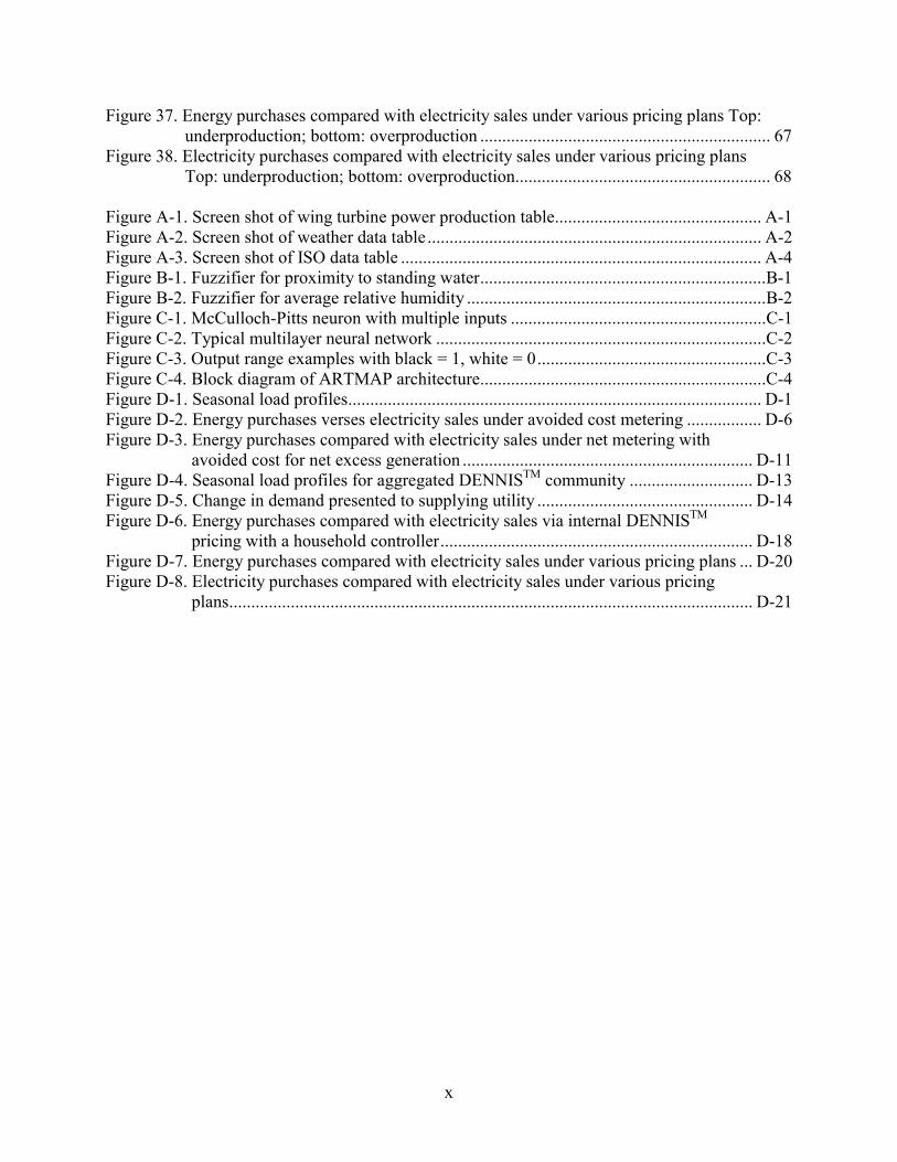
Figure 37. Energy purchases compared with electricity sales under various pricing plans Top: underproduction; bottom: overproduction .................................................................. 67

Figure 38. Electricity purchases compared with electricity sales under various pricing plans Top: underproduction; bottom: overproduction.......................................................... 68

Figure A-1. Screen shot of wing turbine power production table............................................... A-1 Figure A-2. Screen shot of weather data table............................................................................ A-2 Figure A-3. Screen shot of ISO data table .................................................................................. A-4 Figure B-1. Fuzzifier for proximity to standing water.................................................................B-1 Figure B-2. Fuzzifier for average relative humidity ....................................................................B-2 Figure C-1. McCulloch-Pitts neuron with multiple inputs ..........................................................C-1 Figure C-2. Typical multilayer neural network ...........................................................................C-2 Figure C-3. Output range examples with black = 1, white = 0....................................................C-3 Figure C-4. Block diagram of ARTMAP architecture.................................................................C-4 Figure D-1. Seasonal load profiles.............................................................................................. D-1 Figure D-2. Energy purchases verses electricity sales under avoided cost metering ................. D-6 Figure D-3. Energy purchases compared with electricity sales under net metering with

avoided cost for net excess generation .................................................................. D-11 Figure D-4. Seasonal load profiles for aggregated DENNISTM community ............................ D-13 Figure D-5. Change in demand presented to supplying utility ................................................. D-14 Figure D-6. Energy purchases compared with electricity sales via internal DENNISTM

pricing with a household controller....................................................................... D-18 Figure D-7. Energy purchases compared with electricity sales under various pricing plans ... D-20 Figure D-8. Electricity purchases compared with electricity sales under various pricing

plans....................................................................................................................... D-21

xi

List of Tables Table 1. Database Power and Weather Parameters ........................................................................ 7 Table 2. Fuzzy Rule Matrix for Storage Partitioning in DENNISTM............................................ 14 Table 3. Expected Benefit Matrix for a UPS System Supplying Critical Loads Only ................. 17 Table 4. Effect of Discharge Rate and Price Differential on Net Revenue .................................. 21 Table 5. Fuzzy Set Definitions for Normal Fuel Cell Conditions ................................................ 29 Table 6. Fuzzy Set Definitions for Cold Start Fuel Cell Conditions ............................................ 29 Table 7. Fuzzy Model Rule Set for Normal Fuel Cell Conditions ............................................... 30 Table 8. Fuzzy Model Rule Set for Cold Start Fuel Cell Conditions ........................................... 31 Table 9. Relative Magnitude of Harmonics.................................................................................. 37 Table 10. Relative Magnitude of Current Harmonics at 5 A Export ........................................... 39 Table 11. Relative Magnitude of Current Harmonics at 15 A Export ......................................... 40 Table 12. Current Distortion Limits for General Distribution Systems........................................ 41 Table 13. Flow Matrix for Control Law Generator Control Action Outputs................................ 43 Table 14. Relative Cost Performance of Energy Management Systems ...................................... 52 Table 15. Partial Training Data for Neural Network .................................................................... 60 Table 16. Standard Output States.................................................................................................. 61 Table 17. Correct Answer Percentages for Tested Networks ....................................................... 63 Table 18. Net Present Value of Photovoltaic Generation Investment .......................................... 69 Table 19. Net Present Value of Hydrocarbon-Based Generation Investment .............................. 69 Table A-1. Pressure Tendency Codes......................................................................................... A-3 Table D-1. Composite Electricity Price Based on Rate R-1....................................................... D-2 Table D-2. Daily Usage and Price of Electric Power at Residence ............................................ D-3 Table D-3. Savings from Photovoltaic Generation at Avoided Cost.......................................... D-4 Table D-4. Composite Natural Gas Price Based on Residential Rate R-3 ................................. D-4 Table D-5. Savings from Hydrocarbon-Based Generation at Avoided Cost.............................. D-5 Table D-6. Savings from Photovoltaic Generation with Net Metering ...................................... D-7 Table D-7. Savings from Hydrocarbon-Based Generation With Net Metering ......................... D-8 Table D-8. Table D-8. Savings from Photovoltaic Generation With Net Metering and

Avoided Cost Credit for Net Excess Generation ...................................................... D-9 Table D-9. Savings from Hydrocarbon-Based Generation with Net Metering and Avoided

Cost Credit for Net Excess Generation................................................................... D-10 Table D-10. Daily Pricing for Aggregated DENNISTM Community Load .............................. D-13 Table D-11. Savings from Photovoltaic Generation Using DENNISTM Controller ................. D-16 Table D-12. Savings from Hydrocarbon Generation Using DENNISTM Controller ................ D-17 Table D-13. Composite Natural Gas Price Based on Residential Rate R-3 ............................. D-17 Table D-14. Net Present Value of Photovoltaic Generation Investment .................................. D-22 Table D-15. Net Present Value of Hydrocarbon-Based Generation Investment ...................... D-22

1

1. Background of the DENNISTM System Electricity is an indispensable commodity for sustaining modern life. In spite of that, as we launch into the 21st century, electricity continues to be generated by aging power plants that have been retrofitted in attempts to meet environmental standards and distributed through an antiquated system of wires that are managed with pre-1960 control techniques.

Recent deregulation of the electric grid by states and the federal government has sparked wide interest in bringing advanced technology to the power sector. Right now, innovative technologies are poised to disrupt the traditional power market and transform today's one-way power network into a bidirectional energy transfer backbone connecting autonomous groups of generators.

The power industry's vision for the 21st century includes distributed power. Defined simply, distributed power is modular electric generation or storage located near the point of use. Interest in the use of distributed generation (DG) and storage has increased substantially over the past 5 years because of the potential to provide increased reliability and lower-cost power delivery, particularly with customer-sited generation. The advent of customer choice and competition in the electric power industry has, in part, been the stimulus for this increased interest. Also contributing to this trend has been the development of small modular generation technologies, such as photovoltaics, microturbines, and fuel cells. Industry estimates predict that distributed resources (DR) will account for up to 30% of new generation by 2010.

Distributed systems include biomass-based generators, combustion turbines, concentrating solar, photovoltaic systems, fuel cells, wind turbines, microturbines, engine/generator sets, storage, and control technologies. DR can either be grid-connected (grid-parallel) or operate independently (grid-independent). Those connected to the grid are typically interfaced at the distribution system. In contrast to large, central-station power plants, distributed power systems typically range from less than a kilowatt (kW) to a megawatt (MW) in size. Distributed power can produce greater reliability of electric supply, better efficiency in fuel consumption with combined generation of heat and power, improved supply redundancy, wider spread of capital costs in generation equipment, a more diversified mix of energy technologies, and the ability to offset infrastructure investments for transmission and distribution.

As the cornerstone of competition in electric power markets, distributed power will also serve as a key ingredient in the reliability, power quality, security, and environmental friendliness of the electric power system. By supporting customer choice, distributed power may be the long-term foundation of competition in the electric power industry. Now more than ever, the United States must focus on solutions for a secure, reliable, and independent energy supply. The advantages of distributed power promise to significantly reduce the United States' dependence on foreign oil for power generation and home heating and open the door for innovative applications of DG technologies in automobiles and mass transit.

Although the application of DG and storage can bring many benefits, the technologies and operational concepts to properly integrate them into the power system must be developed. The current power distribution system was not designed to accommodate active generation and storage at the distribution level or to allow such systems to supply energy to other distribution customers. The technical issues to allow this type of operation are significant. For example, control architectures to allow safe and reliable distributed power operation, and particularly to exploit the

2

potential for distributed power to provide grid support, will require system protection redesign. This will require large amounts of information fed to intelligent local controllers that can quickly reconfigure and operate local distribution areas for both local and transmission-level benefits.

Orion's solution is an integration system consisting of intelligent, networked household controllers that interact with the electric grid and one another through a single neighborhood “hub” controller. The household controllers maximize return on investment to the purchaser by monitoring utility demand and other parameters to predict future selling and buying opportunities. The neighborhood controller enables bulk electricity transactions on the wholesale market and provides additional power reliability to the entire system. This technology turns a community of distributed generators into a single large generator capable of selling locally generated power in a coordinated manner similar to commercial power plants. Orion’s DENNISTM is a crucial technology for managing the deployment and optimal use of DG. Its intelligent distributed controls empower individuals and cooperatives to make choices in their own best interest.

1.1. The DENNISTM System Diagrams illustrating the proposed design of the DENNISTM system are shown in Figure 1. The household controller contains means for measuring the real-time market price for electricity, the actual load of the household (state of storage and rate of discharge), current weather, and available power from on-site generation sources.

These measurements are fed into a neural network structure that serves as an evolving pattern database that can correlate the measured parameters to established weather, load, demand and available power profiles. The selected pattern can be used to predict trends in all parameters, and therefore, becomes the basis for generating a control law. The control law is chosen using a linear programming algorithm and neural networks, and its main objective is to maximize the potential profit or minimize the cost to the household depending on whether the household is a net seller or purchaser of electricity. By predicting trends in weather and load, the control law can be programmed to take future demand and generation potential into account. The controller will not seek short-term profits at the cost of long-term gains. The controller also contains power-switching circuitry to distribute energy between household storage and the power grid in accordance with the control law.

Figure 1. DENNISTM household (left) and neighborhood (right) controllers

3

Reliability of the system is guaranteed through a tie-in to the neighborhood grid. The Neighborhood Tie-In Controller (NTIC) coordinates the activities of multiple household controllers through real-time pricing signals. The NTIC, shown on the right in Figure 1, monitors weather, load demand within the neighborhood, available generating capacity, the state of a central storage facility, and electricity demand on the power grid. Like a household controller, the NTIC uses neural networks to create a pattern database and learn weather and neighborhood load demands. It uses this information in an optimization routine that acts in conjunction with an intelligent agent for buying, selling, or storing energy based on aggregated neighborhood needs.

The unique aspect of this system is that it allows the neighborhood to act as a small generating company. Because the NTIC is the nexus of an aggregated generation capacity that could be 100 kW to 200 kW for 100 homes, it represents an appropriate block of energy for wholesale trading. The NTIC therefore provides the means for several small power producers to sell their generation to the grid in the most profitable manner.

1.2. Description of Subsystems

1.2.1. Neural Pattern Database The theoretical basis for the Neural Pattern Database is Adaptive Resonance Theory (ART), developed by Stephen Grossberg and Gail Carpenter of Boston University. ART uses feedback between its two layers to create resonance. Resonance occurs when the output in the first layer after feedback from the second layer matches the original pattern used as input for the first layer in that processing cycle. A match of this type does not have to be perfect. Instead, it must exceed a predetermined level, called the vigilance parameter.

An input vector, when applied to an ART system, is first compared with existing patterns in the system. If there is a close enough match within a specified tolerance, then that stored pattern is made to resemble the input pattern further, and the classification operation is complete. If the input pattern does not resemble any of the stored patterns in the system, then a new category is created with a new stored pattern that resembles the input pattern.

In the DENNISTM pattern database, the combined outputs of the system will be used to determine and continuously refine a specific set of operating conditions for use by the Control Law Generator. These outputs will include predictions of available power, weather, load, and demand for the succeeding 24-hour period.

1.2.2. Control Law Generator The Control Law Generator uses a fuzzy rule set to interpret the selected patterns from the Neural Pattern Database and uses these to select an appropriate set of linear constraint equations. These equations represent the following constraints: the need to meet predicted load of the house, predicted generation capacity, cost of generation, and state of capacity of the household storage. An optimization routine based on principles of linear programming determines the operating parameters governing the behavior of the Charge/Discharge Controller. The optimization attempts to maximize return on investment or minimize cost to the owner of a DG resource. A performance-indicating measurement is continually monitored by a dynamic tuning system that perturbs the constraint equations to seek the true optimum operating condition.

4

1.2.3. Charge/Discharge Controller This component is the muscle of the DENNISTM system. The Charge/Discharge Controller contains all the power circuitry necessary to safely transfer electricity among generation sources, storage, and the grid. Its normal mode of operation is governed by the control algorithm generated by the Control Law Generator. The controller contains DC-DC converters to step up or step down voltages between the generation sources and the batteries, an inverter to transfer energy from the batteries to the grid, and a rectifier and charge controller to transfer energy from the grid into storage.

5

2. The Distributed Power Program Subcontract The federal government has an interest and role in the systems aspect of distributed power because of its effects on competition in the electric industry, the reliability and security of the electric power supply, and the environment and because of federal investments in DG and storage technologies. The federal government has also invested heavily in the research and development of DG and storage technologies. As a result, it is important to provide leadership and mission-oriented resources to address the system integration issues that are fundamental to the employment of these technologies in the real world, especially in light of pending deregulation and anticipated changing market and customer needs. The system integration issues related to distributed power are national issues that cut across a number of industries. There is a federal leadership role to bring together these various parties — hardware manufacturers (of photovoltaics, wind turbines, fuel cells, gas turbines, batteries, etc.), utilities, energy service companies, codes and standards organizations, state regulators and legislators, and others — to address the technical, institutional, and regulatory barriers to distributed power. In fact, these very groups have asked for assistance.

The Department of Energy's Distribution and Interconnection R&D has been structured to address overall systems operation, reliability, safety, power quality, and institutional issues. This subcontract to develop, model, and test the DENNISTM household/neighborhood controller approach supports the program's research and development focus of strategic research. Specifically, the project meets the need for automated, adaptive intelligent interconnection and control and technology to enable aggregation, grid support, and ancillary services from DR.

Program Objectives The objective of this subcontract over its 3-year duration is to develop a household controller module and demonstrate the ability of a group of these household controllers to operate through an intelligent neighborhood controller to provide a smart, technologically advanced, simple, efficient, and economic solution for aggregating a community of small distributed generators into a large single, virtual generator capable of selling power or other services to a utility, ISO, or other entity in a coordinated manner.

The goals in Year One were to construct and demonstrate the major subsystems, validate subsystem performance using data collected at the University of Massachusetts Lowell Center for Energy Conversion (UMLCEC), install a fuel cell, and upgrade electronics at UMLCEC. The following technical objectives were pursued to prove the feasibility of the household controller design presented above and explore the economics of the entire DENNISTM system:

• Construct and demonstrate the performance of the main subsystems, including the Neural Pattern Database, Control Law Generator, and Charge/Discharge Controller.

• Analyze the data collected by UMLCEC on the performance of the solar and wind generators to permit proper validation of the Neural Pattern Database performance.

• Develop new neural network and fuzzy models of state-of-the-art PEM fuel cells that will provide an additional source of power when solar and wind energy are not available.

6

• Characterize the harmonic content of the power generated by the wind turbines, solar panels, fuel cells, and switchgear as a function of various parameters such as battery bank voltage and wind speed.

• Modify power-handling systems in the UMLCEC to handle energy transfer among the interconnected DG sources, battery bank, and utility interconnection.

• Develop an assessment of the economic effect of the DENNISTM system.

To meet these objectives, Orion developed a work plan consisting of seven tasks. Each of these tasks is described in detail in the sections that follow.

7

3. Task 1 – Data Reduction and Analysis The purpose of this task was to provide real-world, reliable data to support the development of DENNISTM subcomponents. Orion examined and reduced energy production data gathered over the past 6 years at UMLCEC from its DG capacity. This capacity comprises three wind turbines, a solar array, battery storage, and a utility interconnect. Data have been logged continuously in 5-minute intervals by UMLCEC and include wind speed, wind-generated DC current, wind-generated voltage, insolation, photovoltaic voltage, photovoltaic DC current, battery voltage, AC voltage to utility, AC current to utility, and power delivered to the utility. The data have been strategically arranged within a Microsoft Excel database so that they can be easily categorized, summarized, and reported.

3.1. Basic Structure of the Database The core of the database is a table of raw data collected from UMLCEC. This table contains hourly average measurements of the power and weather parameters listed below.

Table 1. Database Power and Weather Parameters

Column Label and Description Units DATE and TIME mm/dd/yy and hh:mm:ss (24-hour clock) Date and ending hour of hourly data average VBAT DC volts (VDC) DC voltage at the main bus of the storage batteries ABAT Amperes (A) DC current measured on the storage battery mains 300 DCA Amperes (A) DC current delivered by the 300-W wind turbine 500 DCA Amperes (A) DC current delivered by the 500-W wind turbine 1500 DCA Amperes (A) DC current delivered by the 1,500-W wind turbine 300 DCW Watts (W) Power delivered by the 300-W wind turbine 500 DCA Watts (W) Power delivered by the 500-W wind turbine 1500 DCA Watts (W) Power delivered by the 1,500-W wind turbine

8

300 WIND Miles per hour (mph) Wind speed measured by an anemometer installed on the tower of the 300-W wind turbine 500 WIND Miles per hour (mph) Wind speed measured by an anemometer installed on the tower of the 500-W wind turbine 1500 WIND Miles per hour (mph) Wind speed measured by an anemometer installed on the tower of the 1,500-W wind turbine SUN Watts per square meter (W/m2) Insolation measured by a solar cell located at the photovoltaic panel installation MPPT DCV DC volts (VDC) DC voltage of the photovoltaic installation measured at the high-voltage side MPPT DCA Amperes (A) DC current delivered by the photovoltaic installation measured at the high-voltage side INV ACA Amperes – RMS (Arms) RMS AC current delivered to the grid through the inverter at 120 VAC

A number of tables have also been created with values derived from the baseline UMLCEC data to support the various tasks.

3.2. Power Production Tables Power production tables, as illustrated by Figure A-1 in Appendix A, represent the amount of power generated by each device in the UMLCEC facility. The devices listed are the fuel cell; wind turbines rated 300 W, 500 W, and 1,500 W; and photovoltaic panels rated at 2,500 W. An additional table reports the amount of AC electricity exported to the grid.

3.3. Weather Table The weather table (Appendix A, Figure A-2) captures several variables that characterize the current weather in the Lowell/Lawrence region. The Lowell data are collected at each of the generators. Wind speed and direction are recorded at each turbine, and insolation is recorded at the PV bank. Additional data are supplied from National Oceanic and Atmospheric Administration (NOAA) records. NOAA maintains an unattended Automated Surface Observing System (ASOS) weather monitoring station in Lawrence, Mass. Lawrence is located approximately 10 miles from Lowell and experiences substantially similar weather.

3.4. Electric Power Price and Demand Table This table (see Appendix A, Figure A-3) reports data published by the New England Independent System Operator (ISO-NE), the authority that establishes the real-time wholesale price for electricity in the New England region. This table may be expanded in the future to include similar data from California and/or New York.

9

3.5. Section Conclusions The UMLCEC has collected excellent data from 1998 forward and has reasonably complete data from 1994 to 1998. Using additional data pulled from sources such as NOAA and ISO-NE, Orion has been able to create a very complete database of operational data. Efforts to improve and refine the data included in the database will continue throughout the program.

Data on power production was summarized and converted to a set of generation profiles to simulate different types of generation mixes (e.g., a PV-only installation, a PV/wind installation, or a fuel cell installation). These profiles were then assigned an operating cost based on the historical price of fuel. The cost performance was computed using the corresponding daily ISO hourly clearing price and appropriate assumptions about the timing of electricity sales and purchases. The weather data were used to develop and refine weather learning and prediction neural networks.

10

4. Task 2 – Power Electronics 4.1. Facility Upgrades and Enhancements The first activity in this task was to upgrade all power-switching components to enable remote control by computer. This upgrade was necessary to allow automatic control of the power system by the DENNISTM programs running on nearby computers. Figure 2 shows a block diagram of the DENNISTM project installed at UMLCEC, with the power-switching stations (PSS) identified. The PSS are specialized conversion components that convert electric power from one form to another and control the flow of electric power between storage and other conversion components.

Figure 2. UMLCEC distributed power station

4.1.1. Identifying Relevant Power Switching Stations The first step in the DENNISTM integration procedure was to identify which of the power switching stations need control by DENNISTM. In general, these are the PSS controlling energy flow to the utility grid and in and out of storage because the primary function of DENNISTM is controlling power transfer to the grid based on available energy, including stored energy. Only two of the PSS at UMLCEC need to interface with the DENNISTM controller: the renewable energy system (RES) inverter and the fuel cell controller.

Because renewable energy sources such as wind and solar have no fuel cost and operate whenever their energy resource is available, the energy converters for these devices are allowed to operate whenever energy is available. Their energy will either be stored or used, never wasted. The rectifiers and maximum power point trackers associated with the wind and photovoltaic converters are fully automatic devices. Their major role is to match the electrical supply type from the converters to that required by the battery bank and RES inverter.

11

The RES inverter performs the electrical conversion necessary to interface the common DC bus for the laboratory's generation with the utility grid and controls the flow of electrical power in and out of the battery storage unit.

The fuel cell controller performs the same role as the RES inverter: it interfaces the fuel cell electrical output with the batteries and electric grid and controls the flow of power out of the hydrogen storage unit and into the battery storage unit. 4.1.2. Establishing Standard Communications with the Relevant PSS Because distributed power stations may have a variety of configurations and generator types that may be significantly different from the UMLCEC setup, a standardized procedure for interfacing DENNISTM was developed.

The serial communication protocol RS232 was chosen as the standard communication method for the DENNISTM prototype because the protocol is easily adapted to longer distance transmission as RS485 or by modem for remote control and because most sophisticated electronic equipment has provisions for handling serial communication via RS232.

At UMLCEC, the RES inverter has an RS232 option, which was purchased, installed, and tested. The fuel cell PSS is currently being designed with a Motorola 68HC12 microcontroller, which can communicate serially.

Translator program code modules translate a command from the DENNISTM main controller to the specific command sequence required by a particular PSS. Commands from the DENNISTM controller specify the transfer of power to a specific component, at a specified level, in response to certain criteria. For example, DENNISTM may issue a command to sell 2 kW of electricity for 4 hours at the midday peak based on information processed in the DENNISTM modules that predict fuel pricing, load requirements, and weather. The sell command may be contingent on keeping a specified amount of energy on reserve for critical loads in the event of a utility outage. The translator module would issue this “sell” command to the PSS using the appropriate language and protocol.

4.1.3. Section Conclusions The Trace SW4024 Series Inverter (RES Inverter) was identified as the primary PSS to be controlled by DENNISTM. An additional PSS is being developed for the fuel cell. The PSS modulates power flow through energy storage — in this case, a battery bank — to the utility grid. The DENNISTM controller instructs the PSS when and at what power level power transfer operations are to occur.

Communications between DENNISTM and the PSS is established using the RS232 serial communications protocol and can occur through direct cable or by modem or wireless. Communications between DENNISTM and the PSS are handled through translator code modules that use routines written by UML and a third-party, serial-communications software library. This standardized structure allows DENNISTM to communicate with a variety of PSS equipment. Only the specific translator code to process a DENNISTM standard command into a machine-specific format must be developed for each new piece of equipment.

12

To communicate serially with the PSS, the PSS equipment had to be upgraded to a new internal software version. Serial communications were established successfully with the PSS through its native software and through the custom C programming language routines. The translator code module format was developed and tested successfully. The DENNISTM controller now has a standard means of communicating its commands to the PSS, which will then precisely control energy transfer through the utility grid and battery storage.

4.2. Storage Sizing Analysis The next item was to examine the use of storage for decoupling generated electricity from the connected load. In most DG applications, the DG is used in one of two modes. One mode uses the energy to offset customer load, and the other puts the generated electricity directly onto the grid. The mode chosen often depends on the type of DG installed, and traditional installations will generally employ only one strategy based on what is expected to give the best cost benefit.

This process leaves a great deal of guesswork in the economics of the system and ultimately cheats the utility and customer out of more productive uses for the DG asset. For passive generating technologies such as wind and solar photovoltaics, the energy produced is a function of weather, so the generation is typically connected to feed internal loads. Although solar generation tends to coincide with the utility peak demand, the generation uncertainty caused by weather makes it impractical to connect the panels directly to the grid for contract energy resale. Net metering has been used in this mode to provide benefit for the customer, but net metering does not benefit the utility. For DG systems such as internal combustion engines, turbines, microturbines, and large fuel cells, the utility may opt to dispatch the generation for load shedding at times when the grid is congested or demand is especially high. The value of these emergency transactions is determined by special contract with the utility. The generation can also be used by the facility to shave demand and lower utility prices. In each of these cases, the optimal use of the generation resource may not be achieved because of the limited deployment of the source to meet a specialized need.

4.2.1. The Role of Energy Storage Energy storage equipment can be used in a DENNISTM application to decouple the availability of the generation resources with the demands of the load. With storage, DENNISTM can implement many simultaneous strategies, including demand side management applications such as load leveling and uninterruptible power supplies. The DENNISTM system also provides a new opportunity for energy storage in the wholesale or real-time pricing markets: that of reserving power for times when the market is experiencing a supply shortage while also providing a sink for surplus supply. The purpose of this task was to demonstrate the techniques developed to size storage capacity to cost-effectively perform its role in a DENNISTM application. The primary storage methods discussed here are batteries and fuel cells. Fuel cells are considered storage if coupled with electrolysis. 4.2.2. The Role of DENNISTM in Increasing the Realized Value of Excess Generation DENNISTM provides an opportunity for excess generation to be valued at current market rates — not just monthly average avoided cost — and for it to be bid into premium price markets, such as emergency power sales. DENNISTM provides this function by estimating the amount of excess generation available for a certain time period based on predictions of fuel prices, weather, load, and status of energy reserves and then providing a means of communicating this information to a system aggregator. The system aggregator may be the DENNISTM NTIC. The aggregator collects bids on behalf of its member constituents and then bids into the wholesale markets and

13

communicates scheduling information back to the household DENNISTM units. The system aggregator also sets the wholesale and retail energy prices for the portions of the grid under its control based on current internal demand, contracts with outside customers and agencies, and available generation.

The presence of energy storage with each unit of DG allows DENNISTM to decide to temporarily hold excess generation and release what is available when the best financial opportunity appears. The storage can then be recharged from future excess generation or during off-peak hours. Real-time retail pricing provides similar opportunities for DENNISTM-equipped customers to provide power when market prices are highest and consume when they are lowest. Of course, over time and with a large penetration of DENNISTM units on the grid, electricity prices will tend to flatten, and smaller gains will be realized from the buy-low sell-high scenario.

In a grid-independent application, storage for a DG resource is often sized to meet a reliability level, expressed by the loss-of-load probability (LOLP). Because the costs associated with storage can be substantial, the designer is faced with the challenge of balancing the cost of the system with a desired LOLP. A great deal of research has been devoted to the optimal sizing of storage and generation for grid-independent installations. This corresponds with the first mode of operation discussed in the introduction. At this point, the body of research jumps to grid-parallel DG with no storage. If storage is mentioned in relation to these systems, it is to provide load following where the transient behavior of the DG is not fast enough to meet the dynamics of the load.

DENNISTM sits between these two modes in the realm of grid-parallel DG with significant storage. This extra storage allows DENNISTM to perform market-based buy and sell transactions that are not accessible to either of the two other systems. Whereas the energy storage in these other cases is often sized based on worst-case scenarios, the DENNISTM intelligent controller can allocate energy in storage dynamically as needed to realize the maximum benefit from real conditions. DENNISTM will store energy if its monetary value in the next 24 hours is higher than its present monetary value. Determination of energy's value requires consideration of strategies and desires for the energy, including reliability, demand side management, and sale potential.

Accordingly, DENNISTM first determines if the energy available in storage commands the highest value if it is held to help meet customer load at some future time. For example, under demand-side management (DSM) load-leveling strategies, stored energy has a high value if a load peak or on-peak pricing is approaching. For UPS applications, stored energy has a high value if inclement weather makes a generation shortage especially likely. Such a shortage leaves the customer at the mercy of market electricity prices if there is inadequate energy stored to help the customer ride through high price/demand times. On the other hand, stored energy may not be needed in the future if adequate energy is expected to come from renewable resources or the load will be especially low, as during a factory shutdown.

If any portion of the stored energy is not likely to be needed in the near future, DENNISTM determines if it will be more profitable to use that stored energy to offset current load demand or to request a bid into the wholesale market at some future time. Because there are energy loss penalties associated with holding storage for a long time and increased error in long-range predictions, DENNISTM examines the best opportunities within a 24- to 72-hour window.

14

Implementing this type of optimization strategy with a fuzzy control system can enable DENNISTM to decide how to allocate regions of storage for different strategies. With this approach, DENNISTM can provide UPS services, power sales, and demand-side management from a single storage bank. Table 2 shows a fuzzy rule matrix for storage partitioning, and Figure 3 shows the appropriate membership functions for the fuzzy matrix's variables.

A major issue that must be resolved is determining the capacity of energy storage in a DENNISTM application system that ultimately realizes the best economic returns. Energy storage has recharge costs, capital costs, and maintenance costs associated with it, so the benefits from the desired capacity must be carefully weighed. The following section describes the methodology to conduct this analysis.

The sizing of storage ultimately depends on the primary task the storage is intended to perform. The following five scenarios are examined: UPS, peak shaving, real-time pricing, offsetting time-of-use charges, and decoupling the load from energy generation.

Table 2. Fuzzy Rule Matrix for Storage Partitioning in DENNISTM

Future Load Future Price Future Generation Storage Capacity Required

H H L H

H H H M

H L L M

H L H M

L H L M

L H H M

L L L M

L L H L

15

1.0

0.0

HL

GENERATION

1.0

0.0

HL

LOAD

1.0

0.0

HL

PRICE

1.0

0.0

L HM

STORAGE CAPACITY

Figure 3. Membership functions for fuzzy rules

4.2.3. Storage Sizing for UPS Systems UPS systems are usually sized for the worst-case scenario. The worst-case scenario is complete absence of power supply, either from on-site generation or from the grid, for any duration of time. So storage must provide 100% of what is required by the load for that time. The duration of time that the supplies from all sources are expected to be absent is determined by Loss of Load Probabilities.

Generally, loads can be separated into critical, which cause high-value losses if they are not supplied, and non-essential, which cause minimal or convenience-value losses if they are not supplied. The non-essential loads may have a segment identified as semi-critical loads, which means they do not need to be supplied indefinitely but they may cause problems if they are suddenly interrupted. Some examples are computers, lighting, and certain machinery. The UPS system must be able to provide for the semi-critical loads for a short duration of time until they can be safely shed.

The optimum size for energy storage is that which minimizes losses at the least cost. The optimum storage size to minimize loss will also maximize benefit from Bayes’ criterion. The expected benefit of providing an amount of storage is given by:

16

( ) ( )[ ]∑ Ω=Ωj

jijij PE θ (1)

where:

θj represents an actual event

Ωij is the benefit associated with action ai when the actual event was θj

P(θj) is the probability that the event θj will occur.

The optimum storage size is given by:

ai, for MAXi [E(Ωij)/C(ai)] (2)

where:

C(ai) is the cost for action ai.

For a UPS,

θj represents the duration of an outage in minutes

ai is the amount of storage provided

Ωij is the benefit associated with providing storage ai when the loss of supply lasts θj

P(θj) is the probability that the loss of supply will last θj

C(ai) is the cost of storage ai.

In particular,

Ωij = base loss + θj * loss rate (3)

C(ai) = cost/unit * n units (4)

n = ceil [(time/capacity @ discharge rate] (5) where:

“base loss” is the economic loss from any interruption of power, no matter the duration

“loss rate” is the continued economic loss caused by failure to supply critical loads

“time” is the duration the load is supplied

“capacity @ discharge rate” is the time the storage unit can supply the given discharge rate.

17

Table 3 shows an expected benefit matrix for a system with the following properties:

C(ai) = $100/unit * n units

n = ceil [(θj/60)/10] (for discharge @ 10-hour rate to provide power for critical loads)

Ωij = for ai < θj; $100/min * (ai +1)

for ai ≥ θj; $100/min * (θj + 1).

Table 3. Expected Benefit Matrix for a UPS System Supplying Critical Loads Only

0.1 1 10 100 1,000 10,000

0.833 0.083 0.05 0.025 0.008 0.001AvailableStorage Expected Storage Benefit/Cost

(Minutes) Benefit Cost Ratio10 $110 $200 $1,100 $1,100 $1,100 $1,100 $201 $100 2.01

100 $110 $200 $1,100 $10,100 $10,100 $10,100 $507 $100 5.071,000 $110 $200 $1,100 $10,100 $100,100 $100,100 $1,317 $200 6.58

Loss of Supply (Minutes)

Probability of Occurrence

From the table, it can be seen that the optimal storage size is on the order of 1,000 minutes. The actual benefit realized will be less the cost of energy to account for inefficiencies. This can be accounted for by reducing the loss rate accordingly. This table is based on the assumed loss rate. Ultimately, the value of the expected benefit must be determined by what consumers will pay for a specific level of reliability.

4.2.4. Storage Sizing for Peak Shaving The usual objective of owning storage capacity for peak shaving purposes is to avoid the demand charges imposed for providing high power service to the customer. Energy storage and controls can be used to cap the amount of power drawn from the utility grid. If the load requires more power, that power must be drawn from storage, or the load must be reduced. The storage is then recharged over time when the rest of the building load is low. The load factor is the ratio between the peak load and the average load. A high load factor indicates a high peak, which has a short duration. A load factor of unity equals a flat load profile versus time. The peak-shaving strategy realizes the most savings for loads with a high load factor. The specific loads causing the high peak are usually known. The storage can be sized for peak-shaving applications using the same methodology as outlined in the previous section, with the following adaptations:

For peak-shaving,

θ represents the actual size of the peak load, which is known

ai is the amount at which the peak is capped

Ωi is the benefit associated with providing storage to cap the peak at ai with peak load of θ

18

P(θ) is the probability that the peak load will be θ, which is 1

C(ai) is the cost of storage for a cap at ai.

In particular,

( ) ( )

−

−

−

−=Ω ∫ kWh

akW

ah

iii$

11$ θ

ηθ (6)

where:

$/kW is the demand charge

h is the duration of the peak in hours

η is the efficiency of the system

$/kWh is the energy charge.

For a DENNISTM application, such as a municipal utility district fed by a transmission line and substation, the size of the transmission capacity may be limited. Additional power for the district will be met by local generation and storage tied in at the distribution level. This is done to provide savings for ratepayers in the district. The generation in the system is designed to meet some fraction of the maximum load based on knowledge of load diversity, and some required safety margin is provided. Storage is therefore being used as bidirectional spinning reserve, and the size is dictated by the system rule-of-thumb requirements. The optimal size for storage will depend on the economics of the alternatives for spinning reserve. The benefits for storage in this system equal the revenue received for the energy released from storage. Other benefits are reduction in stress on other generators.

4.2.5. Storage Sizing for Real-Time Pricing Under a real-time pricing scenario, a customer would be encouraged to conserve power when prices are high. In a DENNISTM system, the additional possibility exists of transferring power to the grid when prices are high and more supply is most needed to receive the best monetary compensation for that power. If energy storage is present in the customer’s system, then energy can be released from storage when prices are high and the storage replenished when prices are low.

The following methodology optimally sizes storage for a buy-low sell-high scenario for DENNISTM-equipped energy storage. An assumption for this methodology is that electricity prices follow periodic daily and seasonal cycles in addition to linear annual inflation and other random influences.

The first step is to determine the equation describing historical electricity prices. Wholesale prices are used for this analysis and are assumed to be similar to real-time prices. Figure 4 shows wholesale price variations over the year 1998. Figure 5 shows a close-up view of a particular day, including process action limits.

19

$0$10$20$30$40$50$60

130

160

190

112

0115

0118

0121

0124

0127

0130

0133

0136

0139

01

Cos

t ($/

MW

)

3999

4253

4507

4761

5015

5269

5523

5777

6031

6285

6539

6793

7047

7301

7555

7809

Hour of the Year 1998

7999

8253

8507

Figure 4. Cost to serve the next megawatt of load for 1998

$0

$10

$20

$30

$40

$50

$60

1 3 5 7 9 11 13 15 17 19 21 23Hour

Who

lesa

le P

rice

($/M

W)

Figure 5. Example of electric wholesale daily price fluctuations for June 11, 1998

The forecast for wholesale electric prices for the next hour is given empirically by:

Y = b0 + b1t + b2sin 15t° + b3cos 15t° + b4sin 0.082t° + b5cos 0.082t° (7)

where:

Y is the forecast wholesale electricity price

t is the next hour of the year

b0 - b5 are the fitted coefficients describing the trend of electricity price.

The next step is to determine the process action limits. DENNISTM will generate an automatic release command when the electricity price rises above the high limit, and an automatic store command will be issued when the electric rate drops below the lower limit. Process action limits can be set to take advantage of daily cyclical fluctuations or to take advantage of the price spikes during the year. Long-term trends can be removed from the data using the forecast equation.

20

In general, it would seem that the best economic gain is realized when the process limits are set as close as possible to the peaks. DENNISTM should release as much power as possible at the highest possible price and store as much power as possible at the lowest possible price. As the process limits are shifted closer to the average value, more units of power will be released at lower prices, and more units of power will be stored at higher prices, decreasing returns.

The amount of storage capacity for the system therefore seems to be limited only by the maximum amount of power that can be transferred during the smallest time block and the capital cost a person is willing to invest. Larger systems are favored because of their better cost-power ratio. The number of storage units required to provide this power is sized based on the units’ maximum discharge rate.

However, this is usually not the optimum situation. First, the utility company is not likely to want a huge, sudden spike of power on its lines and may levy financial penalties for such behavior. Second, the effective capacity of storage, especially if it is a battery bank, changes with respect to the discharge rate. In addition, the life span of the storage may be reduced significantly if it is repeatedly charged and discharged at peak rates. Therefore, the same initial capital investments on the same physical units may have very different ROIs for systems operated differently.

With this in mind, the optimum storage capacity for a DENNISTM-equipped energy storage system is given by first determining the optimum discharge rate and process action limits for a single unit. The optimum discharge rate is the one that realizes the best revenue per storage unit. The process action limits are perturbed closer to the average price. This represents longer discharge times at lower rates. The capacity of a single storage unit operated under these conditions is then determined. The benefit of operating the storage unit under these conditions is determined from the net value of the energy transferred, and the best combination is identified.

The pricing information used to run this analysis is the typical pricing for the time period for which optimization is desired. Generally, optimization will be desired daily, weekly, or seasonally. The total number of units in the system is still limited by the power transfer capability of the connecting equipment and capital cost.

The benefits are given by:

( )( )kWhPPR SR −∆= (8) where:

R is net revenue for energy released from storage ∆(PR – PS) is the average price differential between power bought and power sold PR is the average price received for power released from storage PS is the average price spent on power stored kWh is the amount of power transferred, corresponding to a given discharge rate.

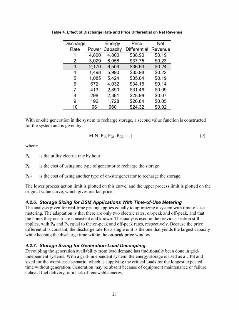
Table 4 shows an example of a system with battery storage. Two opposing forces are at work. The energy transferred (kWh) tends to increase with lower discharge rates and longer discharge times, but the average price differential decreases. As shown in the table, the best revenue per storage unit is at the 3-hour discharge rate, and each unit provides 2 kW.

21

Table 4. Effect of Discharge Rate and Price Differential on Net Revenue

Discharge Rate Power

Energy Capacity

Price Differential

Net Revenue

1 4,800 4,800 $38.90 $0.192 3,029 6,058 $37.75 $0.233 2,170 6,509 $36.63 $0.244 1,498 5,990 $35.98 $0.225 1,085 5,424 $35.04 $0.196 672 4,032 $34.15 $0.147 413 2,890 $31.46 $0.098 298 2,381 $28.98 $0.079 192 1,728 $26.84 $0.0510 96 960 $24.32 $0.02

With on-site generation in the system to recharge storage, a second value function is constructed for the system and is given by:

MIN [PU, PG1, PG2, …] (9)

where:

PU is the utility electric rate by hour

PG1 is the cost of using one type of generator to recharge the storage

PG2 is the cost of using another type of on-site generator to recharge the storage.

The lower process action limit is plotted on this curve, and the upper process limit is plotted on the original value curve, which gives market price. 4.2.6. Storage Sizing for DSM Applications With Time-of-Use Metering The analysis given for real-time pricing applies equally to optimizing a system with time-of-use metering. The adaptation is that there are only two electric rates, on-peak and off-peak, and that the hours they occur are consistent and known. The analysis used in the previous section still applies, with PR and PS equal to the on-peak and off-peak rates, respectively. Because the price differential is constant, the discharge rate for a single unit is the one that yields the largest capacity while keeping the discharge time within the on-peak price window. 4.2.7. Storage Sizing for Generation-Load Decoupling Decoupling the generation availability from load demand has traditionally been done in grid-independent systems. With a grid-independent system, the energy storage is used as a UPS and sized for the worst-case scenario, which is supplying the critical loads for the longest expected time without generation. Generation may be absent because of equipment maintenance or failure, delayed fuel delivery, or a lack of renewable energy.

22

In a grid-interactive DENNISTM application, decoupling the generated energy from the load demand energy is accomplished by providing enough energy storage to hold the daily excess generation until some specified future date. At that time, it will either be used to meet load and will be valued at retail pricing, or, if it still is excess, it will be made available for sale on the wholesale market. This arrangement gives DENNISTM owners the freedom to do whatever they want with their excess generation (i.e., they can use it immediately or later). Obviously, one does not need to hold the entire excess for the day or limit the storage size to the excess of one day. The daily time constraint is a design specification of DENNISTM, and storage is sized accordingly.

The storage sizing method for DENNISTM operation will be a basic dynamic optimization in which a strategy for a range of operation is decided at once. The cost function for the benefit provided by storage is formulated as:

( ) ( )

×−×= ∑

=

N

kkkkkDUopt UPQDC

kk 1,max (10)

subject to the following constraints for k = 1 to N hour-long periods

kkkk WUXX −+=+1 (11)

0XX N = (12)

kk UU max,≤ (13)

maxXX k ≤ (14)

0≥kU (15)

0≥kX (16)

where the symbol X refers to storage, U refers to electricity consumption, and W refers to demand for electricity. The demand comprises internal load, L, and external demand, D, such that:

kkk DLW += . (17)

The electricity consumption over the 24-hour period, U, for a given demand is chosen by solving the optimization problem in equations 18 through 24. The constraint in Equation 12 ensures that the energy used over the 24-hour period in W is replaced by an equal amount of energy from U. Equation 13 constrains the energy consumption in any period to less than the value of Umax in that particular period. The value of Umax in any interval is provided by analysis of the neural pattern database predictions of available generation, power from the grid, or hand-off power from an area of storage for another function. Equation 14 constrains the amount of stored energy to the amount of available storage. The optimal value of Xmax is chosen iteratively prior to each optimization step. The benefit-to-cost ratio for each value of Xmax can be calculated for each iteration with Xmax using typical day parameters for the site. The optimal value of Xmax will have the highest benefit-to-cost ratio.

23

4.2.8. Section Conclusion Orion developed several methods for optimally sizing storage with and without a DENNISTM unit for the following applications: UPS, DSM peak shaving, DSM time-of-use offset, real-time pricing, and decoupling generation from load. For UPS applications, Orion developed a framework for comparing system benefits and costs using Bayes' criterion. Using modest benefit functions, the optimal storage size for a loss rate of $100/min was found to be about 1,000 minutes. Ultimately, however, the true cost-benefit function can only be generated with a complete knowledge of system outage probabilities and a free-market value for reliability.

DSM applications use a methodology in which the dollar savings in demand charges are balanced against the dollar costs in kWh to make up the difference between actual and capped demand. The optimal storage size is that which produces the highest savings on the cost function compared with storage cost. The actual size of storage has to be determined in situ. For real-time pricing applications, a methodology was developed for sizing storage using historical price predictions and natural process limits. In this context, it was discovered that the quantity of energy bought and sold is constrained by the discharge rates of the storage technology and/or utility limits on maximum discharge of energy from storage. Using a method that balances best buy/sell price points against safe discharge rates for batteries, it was determined that a 3-hour discharge rate is optimal. Storage capacity is approximately 6.5 kWh. Storage sizing for load decoupling is determined by an optimization over 24 to 72 hours. The optimizing cost function balances the cost of electricity supplied from DG or the grid with cost benefits supplied by any of the three strategies examined above.

In the end, it was concluded that there are no cut-and-dried formulas for computing the optimal storage size without detailed knowledge of the site and its rate structures. Although it was possible to estimate storage sizes based on assumptions about market rates, these are approximations at best. The fundamental conclusion is that DENNISTM may need to be deployed with oversized storage, and the DENNISTM system can then partition that storage among the three strategies as it learns the neighborhood market patterns. If, for example, DENNISTM is installed with 10 kWh of storage, it may discover through its optimization routines that it should dedicate1 kWh to UPS, 2 kWh for DSM, and 4 kWh for real-time pricing. The remaining 3 kWh could be used as storage for neighborhood-level transactions, with control of that block handed off to the neighborhood DENNISTM controller. The available storage for the neighborhood controller would therefore not be a solid block at one location but consist of several smaller blocks distributed among all the households inside the DENNISTM neighborhood. This strategy may reduce the transportation of electricity on the grid because the neighborhood controller will often charge its storage from individual households. Instead of each house dispatching electricity to the grid for central storage, they can instead charge the portion of storage dedicated to neighborhood transactions.

There is now a working set of equations and a methodology for performing storage optimization at any DENNISTM site. The DENNISTM approach will ensure better use of any DG asset than is currently possible with pre-engineered DG systems. The dynamic allocation of storage among several competing strategies ensures that the system is optimally configured for making money even when utility conditions change.

24

5. Task 3 – Fuel Cell Characterization and Integration 5.1. Fuel Cell Installation and Commissioning A 500-W fuel cell was added to the existing facilities at UMLCEC to serve as an immediately dispatchable generation source. The ability to operate the fuel cell at any time complements the weather-dependent solar and wind generators already installed at the site. The fuel cell has the added benefit of serving as a renewable resource with energy storage if the hydrogen is manufactured by renewably powered electrolysis and stored in devices such as metal hydride solid-state storage. 5.1.1. Selection The fuel cell was chosen to be large enough to reasonably represent a possible residential system and to be on the same order of magnitude as the other generators in the system but not to be so large as to overload the existing electrical power system. Additional criteria for selection were that the fuel cell had to: be commercially available, have minimal operation and maintenance requirements, be feasible inside a public building with adjacent classrooms, and have a cost within the project budget. The fuel cell chosen was the PS500 PowerPEM from H Power.

5.1.2. Hydrogen Supply Hydrogen is a colorless gas with no odor. It is not toxic; the immediate health hazard is that it may cause thermal burns. It is flammable and explosive in mixtures of between 4% and 75% hydrogen. Hydrogen may react violently if combined with oxidizers, such as air, oxygen, and halogens. Hydrogen is an asphyxiant and may displace oxygen in a workplace atmosphere. However, the concentrations at which flammable or explosive mixtures form are much lower than the concentration at which asphyxiation risk is significant.

Because a 4% concentration (by volume) of hydrogen gas in a room is extremely flammable, and because it is stored under high pressure in the prototype system, the first step of installing the fuel cell was to establish the safety requirements and allowable system parameters. This was done with the supervision of the university’s Department of Work and Safety and Plant Services Department. It included determining the applicable requirements as dictated by the National Fire Protection Agency and developing a standard operating procedure for the fuel cell. Based on the requirements, the use of a 500-W fuel cell system was approved, a limitation on the amount of on-site hydrogen pressurized storage was established, and major modifications to the facility were undertaken. The main portion of the modifications was to construct an isolated, explosion-proof ventilation system and vent hood to exhaust any hydrogen to the outside, above roof level, where it is harmlessly diluted in the atmosphere. Part of this construction involved asbestos removal. 5.1.3. Installation and Training Because of initial problems with manufacturing the PS500, the ship date of this fuel cell model was significantly delayed. The university’s Work and Safety Department and Plant Services Department would not begin design work on the mechanical system until a fuel cell arrived. The discovery and subsequent remediation of asbestos-containing materials in the vicinity of the fuel cell created additional time delays. This remediation was necessary because the existing hydrogen ventilation fan system was not capable of servicing the expanded flow requirements of an additional ventilation hood. UMLCEC spent approximately $20,000 in unbudgeted funds to design and upgrade the ventilation facilities.

25

When the 500-W PowerPEM finally arrived, a hydrogen supplier was chosen. After verifying the ventilation system was satisfactory, the supplier outfitted the facility with a hydrogen cylinder, piping, a two-stage adjustable pressure regulator with gauges, and a flash suppressor. At installation, the system was checked for leaks, and the designated personnel were trained to use the system. Figure 6 shows the installed fuel cell, and Figure 7 shows an interconnection diagram of the system.

The area around the hydrogen cylinder was cleared and painted bright yellow to keep the area clear of objects and combustible materials. Appropriate signs, Materials Safety Data Sheets, and emergency contact information were posted. The facility was already equipped with the appropriate fire-extinguishing equipment.

Figure 6. Installed fuel cell

26

H2

Fuel Line

Fuel Cell

Fused Safety Switch

Fuel Line

To Battery To PC

DC/DC Converter

DAS Transducers &Signal Conditioning

ElectricalOutput

FlashSuppressor

Two-stage pressureregulator:

Tank to 4,000 psi, then4,000 psi to 20 psi

To Roof

Vent Hood

From Batteries

Figure 7. Interconnection diagram of fuel cell system

5.1.4. Testing Following the installation, training, and final approval of the university's Work and Safety Department, the fuel cell was tested for proper operation. A variable load was constructed from electric resistance heat. The load was constructed in modules that could be wired in series and parallel combinations to supply various load combinations to the fuel cell. The fuel cell voltage and corresponding current were measured for each load combination and compared with manufacturer specifications.

Initial tests (see Figure 8) showed the fuel cell output was well below specifications. The fuel cell managed to produce electric power up to 50% of rated output before the load rating was exceeded. After extensive discussions with H Power, the problem was discovered to be a faulty power regulator. After replacement of the defective part, the fuel cell produced rated power.

27

30

35

40

45

50

55

60

65

0 2.5 5 7.5 10 12.5 15

Fuel Cell Current (Amps)

Fuel

Cel

l Vol

tage

(Vol

ts)

Manufacturer's Curve Test Data

Figure 8. Measured fuel cell operating curve versus manufacturer's specification

5.2. Fuel Cell Fuzzy Logic Model With intelligent control and dispatch of generation such as that provided by the DENNISTM system, the output of fuel-based generators is controlled based on the perceived future value of power outputs. To accurately determine that value, the DENNISTM system must know the relationship between power output and fuel input. In addition, the dynamics and methods for on/off and power level control must be fully characterized to achieve proper delivery of power when it is needed.

In this task, a fuzzy logic-based model was developed for the fuel cell system installed at UMLCEC. The model allows DENNISTM to determine the duty cycle of the PSS interface needed to produce the desired power output and determines the amount of hydrogen fuel that will be used. The model was developed using a technique that translates the manufacturer’s specifications into a fuzzy model. The advantages of this approach are that it is fast and standardized and can be easily adjusted after the fact using actual test data. In the DENNISTM system, the parameters of the fuzzy model will be adjusted online using performance data from actual generators.

5.2.1. Fuel Cell System Description The fuel cell is connected to the main power system DC bus through a DC-DC converter labeled Power Switching Station #2 (PSS2). The power system DC bus is a stiff 24-V system maintained by a large-capacity battery bank. PSS2 is a computer-controlled DC-DC converter that regulates the voltage on the fuel cell output side of the system. By varying the fuel cell output voltage, PSS2 is able to achieve some amount of control over the power output of the fuel cell stack. In this way, the power level of the fuel cell is kept within proper operating limits and can be moved to various set points if necessary. A diagram of the system is shown in Figure 9.

28

DC Bus

Battery Storage

65 VDC

24 VDC

24 VDC

120 VAC,1 φ

Grid

Fuel Cell Stack

Hydrogen Supply

Figure 9. Fuel cell system at UMLCEC

5.2.2. Fuzzy Model

Function of the Fuzzy Model Based on the desired power level, as determined by the DENNISTM scheduling algorithm, the fuzzy model determines the corresponding fuel cell operating point (voltage and current), the PSS2 duty cycle to obtain this operating point, and the hydrogen fuel use.

For the UMLCEC system, the fuzzy model has been developed to predict fuel cell current, fuel cell voltage, PSS2 duty cycle, and hydrogen flow rate under cold start and normal operating temperatures. Both fuzzy models are run for a given desired power level. A second stage in the fuzzy model uses actual measured temperature (or expected operating temperature for predictions) as an input to determine the degree to which each of the two possible results applies to current (or expected) conditions. This strategy minimizes the number of rules and number of comparisons that must be made to determine the applicability of each rule.

The fuzzy model linearly interpolates between test operating condition data points. When there is a straight-line relationship between input and output, only the beginning and end points are needed in the model. However, the relationship between the data points for the fuel cell are not linear because of factors such as efficiency and temperature of the fuel cell.

When operating conditions are functions of other variables, such as temperature or battery state of charge, the fuzzy model described above is partitioned and duplicated for each significant operating condition, and then a second fuzzy model is used to interpolate between the possible resultant values. Alternatively, a second fuzzy model can be used to modify the results of the first model. Speed of real-time execution, as determined by the number of operations, will determine the method used.

29

The purpose of the model is to provide accurate predictions of fuel cell performance for the computations performed in the DENNISTM Control Law Generator. Real-time modification of the PSS2 duty cycle in response to battery state of charge is done with an analog or digital feedback loop using terminal voltages at the DC bus and fuel cell output.

Background The basis of fuzzy logic is the fuzzy set. It allows one to define degrees of truth or fitness as opposed to the 'crisp' true/false or probabilistic memberships of traditional sets. The approach for the fuel cell fuzzy model uses the elements of the fuzzy set theory described in Appendix B.

Fuel Cell Fuzzy Model Approach The individual sets are operating data provided by the manufacturer, shown in Table 5 and Table 6. During fuzzification, a desired output power level is mapped to membership in the set described by each of the operating points.

Table 5. Fuzzy Set Definitions for Normal Fuel Cell Conditions

Current Voltage Duty Cycle Hydrogen Flow Desired Power(A) (VDC) (L/min) (% Max)

Set 1 0 60 0.4 0 0Set 2 2.5 54 0.44 1.9 27Set 3 5 52 0.46 3.6 52Set 4 7.5 50 0.48 5.3 75Set 5 10 48 0.5 6.7 96Set 6 12.5 46 0.52 8.1 115Set 7 15 44 0.55 9.2 132

Table 6. Fuzzy Set Definitions for Cold Start Fuel Cell Conditions

Current Voltage Duty Cycle Hydrogen Flow Desired Power(A) (VDC) (L/min) (% Max)

Set 1 1.6 52 0.46 0.9 17Set 2 3 50 0.48 1.8 30Set 3 6 40 0.6 3.1 48Set 4 6 40 0.6 3.1 75Set 5 6 40 0.6 3.1 96Set 6 6 40 0.6 3.1 115Set 7 6 40 0.6 3.1 132

Relating this concept to traditional mathematics, one could say that each of the fuzzifiers is mapping the scalar power level input to an N-dimensional vector space, where N is the number of fuzzy sets. The fuzzifier mapping essentially interpolates the value of the output vector from the basis functions described by the fuzzifier.

Figure 10 shows the fuzzifier for normal temperature operating conditions, and Table 7 shows the rule set used in the fuzzy model to determine the fuel cell system operating conditions for a desired power level. The values in Table 7 are computed by multiplying the current, voltage, etc., level of each set by the point's membership in each set. In the case of 65% desired power level, the point has 52.2% membership in Set 3 and 47.8% membership in Set 4.

30

Set 1

0

0.2

0.4

0.6

0.8

1

0 10 20 30 40 50 60 70 80 90 100 110 120 130 140

Desired Power Level (%)

Mem

eber

ship

Gra

de

0 60 0 0 0

2.554

0.441.90

552

0.463.60

7.550

0.485.30

1048

0.506.70

12.5 46 0.52 8.1 0

15 44

0.55 9.2 0

Current Voltage

Duty Cycle Hydrogen Flow

Set 2 Set 3 Set 4 Set 5 Set 6 Set 7

Figure 10. Fuzzifier for normal fuel cell conditions

Table 7. Fuzzy Model Rule Set for Normal Fuel Cell Conditions

Antecedent Consequent IF desired power is 27%, THEN Fuel cell current = 2.5 A

Fuel cell voltage = 54 V

PSS2 duty cycle = 0.44

Hydrogen flow rate = 1.9 L/min IF desired power is 65%, THEN Fuel cell current = 6.4 A

Fuel cell voltage = 50.9 V

PSS2 duty cycle = 0.47

Hydrogen flow rate = 4.6 L/min IF desired power is 115%, THEN Fuel cell current = 12.5 A

Fuel cell voltage = 46 V

PSS2 duty cycle = 0.52

Hydrogen flow rate = 8.1 L/min

31

The model can also be modified to account for a range of temperature effects or other operating conditions, as shown in Figure 11 and Table 8. The fuzzy model for cold start after long periods of disuse was developed from UML test data and uses arbitrary hydrogen fuel conversion efficiencies for example only. This model assumes that the fuel cell desired power level would not be reachable at initial start-up. When the duty cycle is increased to transfer more power, the fuel cell voltage drops below acceptable levels so that the power transfer level is temporarily capped.

0

0.2

0.4

0.6

0.8

1

0 10 20 30 40 50 60 70 80 90 100 110 120 130 140

Desired Power Level (%)

Mem

eber

ship

Gra

de

1.652.460.90

350.481.80

640.603.10

CurrentVoltage

Duty cycleHydrogen Flow

640.603.10

640.603.10

640.603.10

640.603.10

Set 1 Set 2 Set 3 Set 4 Set 5 Set 6 Set 7

Figure 11. Fuzzifier for cold start fuel cell conditions

Table 8. Fuzzy Model Rule Set for Cold Start Fuel Cell Conditions

Antecedent Consequent

Fuel cell current = 3 A IF desired power is 30% AND operating temperature is LOW, THEN Fuel cell voltage = 50 V PSS2 duty cycle = 0.48 Hydrogen flow rate = 1.8 L/min

Fuel cell current = 5 A IF desired power is 42% AND operating temperature is LOW, THEN Fuel cell voltage = 43.3 V PSS2 duty cycle = 0.56 Hydrogen flow rate = 2.7 L/min

Fuel cell current = 6 A IF desired power is 115% AND operating temperature is LOW, THEN Fuel cell voltage = 40 V PSS2 duty cycle = 0.60 Hydrogen flow rate = 3.1 L/min

32

5.2.3. Fuzzy Model Results Figure 12 and Figure 13 show the outputs of the fuzzy model for any desired fuel cell power level. This model was developed using the manufacturer’s specifications and assumes that the output values are a function of power level and temperature only. The existing membership functions, as shown in the fuzzifier diagrams of Figure 10 and Figure 11, create nearly linear outputs under normal operating conditions and distinctly nonlinear outputs in cold-start conditions.

0

10

20

30

40

50

60

0 50 100 150

Desired Power Level (%) Cur

rent

(A),

Volta

ge (V

), H

ydro

gen

Fl

ow (L

/min

)

Current Voltage

Hydrogen Flow

Current - Cold Start

Voltage - Cold start

Hydrogen Flow -Cold Start

Figure 12. Fuzzy model results for fuel cell operating conditions

0.00 0.10 0.20 0.30 0.40 0.50 0.60 0.70 0.80 0.90 1.00

0 50 100 150

Desired Power Level Cur

rent

(A),

Volta

ge (V

), H

ydro

gen

Fl

ow (L

/min

)

Duty Cycle

Duty Cycle -Start

Figure 13. Fuzzy model results for required PSS2 duty cycle

33

5.2.4. Section Conclusions A working fuzzy model was developed to determine the output voltage and current of the fuel cell, the duty cycle of the DC-DC converter needed to produce the desired power output, and the amount of hydrogen fuel that will be used. Initial results are limited by available data, but the model has proved to be very flexible and readily adaptable for any need that may arise.

In the DENNISTM system, the desired power output is signaled from the main algorithm. An accurate fuzzy model of the fuel cell system allows DENNISTM to accurately predict the cost and energy performance of the system with the fuel cell functioning. The ability to update and train the fuzzy model based on new data will be a considerable asset to the system.

The model was developed using a technique that translates the manufacturer’s specifications, operator’s long-term experience, and specific laboratory test results into a fuzzy model that interpolates linearly in real-time between the different test conditions to account for any desired operating value. The advantages of this approach are that it is fast and standardized and can be easily adjusted.

Further validation of the fuzzy model will occur as more DENNISTM equipment is built into the system at the UMLCEC laboratory. The tests will involve measuring hydrogen flow rate, fuel cell temperature, current, and voltage for different PSS2 duty cycles during fuel cell warm-up and operation. Using this data, more accurate fuzzifiers and fuzzy rule sets can be derived for normal and cold-start conditions. Also planned is an algorithm to automatically update a baseline fuzzy model as more data become available to the DENNISTM system. The controlled laboratory measurements in Year Two will be used as a benchmark for that algorithm.

34

6. Task 4 – Power Quality Study and Control Switches Orion measured and characterized the harmonic content of the multisource generation facility at the UMLCEC. This analysis focused on the characterization of total harmonic distortion (THD) from individual generation resources at UMLCEC and the interfacing of these resources to the utility interconnect. From this analysis, Orion could then take steps to ensure that the power produced by the laboratory system would meet power quality standards set forth by IEEE standards 519 and 1547.

6.1. Introduction A key component of both the technical viability of DG systems and interconnection agreements is the power quality of generation systems where they interface with sensitive appliances and the utility grid. The voltage and current waveforms must be sinusoidal with a minimum of distortion, and the frequency and amplitude of the supply voltage waveform must be within specific limits. Some of these requirements are dictated for DG systems with aggregated capacity under 10 MVA by IEEE P1547 Standard for Interconnecting Distributed Resources with Electric Power Systems. Recommended power quality levels are described in IEEE 519 IEEE Recommended Practices and Requirements for Harmonic Control in Electrical Power Systems. Power quality requirements for an installation may also include specifications for ensuring the number and duration of power outages are kept below a certain level.

Current harmonics are generated by many different types of equipment, such as static power converters, static VAR compensators, inverters, electronic phase control systems, and switch-mode power supplies. Each of these processes contains nonlinear loads that distort the current waveform. The ultimate effect of these current distortions on the voltage waveform depends on the impedance, reactance, and loading of the specific line to which the equipment is attached.

The hazard created by electric power system harmonics is a function of the susceptibility of the equipment attached to the system. Heating equipment is generally the least susceptible, and equipment that requires a perfect sine wave is most susceptible.

According to IEEE 519, harmonic voltages and currents can cause increased heating in rotating machines because of iron and copper losses. They also can give rise to higher audible noise emission. Harmonic pairs, such as the 5th and 7th harmonics, can give rise to mechanical oscillations and place undue stress on rotors. These higher-order harmonics can even induce current in rotors, which can create heating and pulsating or reduced torques. The overall effect is a loss of efficiency and reduction of rotating machine life. Similarly, harmonic currents cause heating and reduced efficiency in transformers. The higher-frequency components may also increase the amount of audible noise. Power cables can be subjected to stress and corona and experience heating beyond normal operation. Capacitors are loaded by higher-frequency components and, therefore, experience greater heating and dielectric stresses in a system with higher-order harmonics.

Power electronic equipment may malfunction when exposed to higher-order harmonics. This equipment is often dependent on accurate determination of voltage zero crossings or other aspects of the voltage wave shape. Distortion causes these points to shift. Electronic equipment can malfunction in subtle ways when fed by power with significant distortion.

35

Current harmonics are of particular concern because of their degrading heating and torque effects on electrical equipment and interference with communications circuits. Low-frequency harmonics are the most difficult to filter out and cause the most problems.

Evaluation of the effects of current harmonics must be done on a case-by-case basis because specific characteristics of each system determine how it will react to high-frequency components. Systems may exhibit resonance modes near certain multiples of the fundamental frequency that will exaggerate the effects of voltage or current harmonics. Reactive elements in the system may work to damp the effect of higher-frequency components, or they may form oscillating tank circuits. Sensitive equipment attached to the line may fail or malfunction when presented with certain combinations of harmonic frequency. Fundamentally, the amount of distortion in the voltage waveform that occurs as a result of nonlinear loads on the line is a function of the type of loads attached, how they interact on the line, and the behavior of reactive and resistive devices on the line.

6.2. UML System The prototype power system at UMLCEC is fed by a 2.5-kW photovoltaic array, three wind turbines rated at 2.3 kW, and a 500-W fuel cell. All power generated by these devices is fed onto a stiff 24-VDC bus anchored by a large set of batteries. A Trace SW4024 inverter fed from the DC bus provides the AC connection to load appliances and the utility grid. A diagram of the system is shown in Figure 14.

BatteryStorage

24VDC

120VAC,1φ

Grid

Fuel CellStack

DC Bus

PhotovoltaicArray

WindTurbines

Figure 14. Block diagram of UMLCEC DG system

Because the Trace inverter is the point of common coupling (PCC) of the UMLCEC system with the utility grid, the study of power quality can be confined to that component and its direct connection with the utility circuit.

The inverter is certified to meet UL 1741, which states that it has been tested in accordance with the UL procedure to verify the inverter meets the requirements of IEEE 929. From this alone, one

36

might assume that power quality would not be an issue. Nevertheless, the Orion team felt it wise to verify that the manufacturer’s specifications are applicable with the inverter connected to the UML prototype system.

The inverter is currently set up as a grid-connected system with an optional attached load. Under normal operating conditions, the load is not connected, and all power produced by the inverter is injected onto the grid. Therefore, the power quality of the inverter output voltage waveform shape, amplitude, and frequency is identical to that of the utility grid.

The power quality item of concern, then, is the harmonic content of the current waveform injected onto the grid by the inverter. Current harmonic content is of special interest in the UML system because the inverter acts as a gateway, transmitting power from other sources through to the utility power grid. It is possible that the inverter would inject not only its own harmonics but also harmonics generated by these other sources. This is especially likely with wind turbines, which generate power at a low-frequency AC most of the time.

6.3. Results The first measurement was a baseline voltage at the inverter output with the inverter outputting no power. Figure 15 shows the baseline utility voltage at the PCC. It is substantially sinusoidal, with only minimal higher-order harmonic content. Figure 16 shows the frequency spectrum of the voltage signal through the 13th harmonic. The relative magnitudes of the harmonics in the voltage waveform are listed in Table 9.

-200.0

-150.0

-100.0

-50.0

0.0

50.0

100.0

150.0

200.0

0.0 3.4 6.9 10.3

13.7

17.2

20.6

24.0

27.5

30.9

34.3

37.7

41.2

44.6

48.0

51.5

54.9

58.3

61.8

65.2

68.6

72.1

75.5

78.9

82.4

85.8

89.2

92.6

96.1

Time (ms)

Volts

Figure 15. Time domain voltage waveform with inverter off

37

0.00%

10.00%

20.00%

30.00%

40.00%

50.00%

60.00%

70.00%

80.00%

90.00%

100.00%

0 28 56 84 112

140

168

196

224

252

280

308

336

364

392

420

448

476

504

532

560

588

616

644

672

700

728

756

784

Frequency (Hz)

Rel

ativ

e A

mpl

itude

Figure 16. Frequency spectrum of voltage waveform with inverter off

Table 9. Relative Magnitude of Harmonics

Harmonic

Frequency (Hz)

Relative Magnitude

Fundamental 60 1.000

3rd 180 0.014

5th 300 0.023

7th 420 0.005

9th 540 0.002

In the next set of measurements, the objective was to measure the current and voltage waveforms for the inverter at different output current settings. If harmonics are present in the current waveform, then measuring these at different output current amplitudes indicates how the waveform scales and shows the ability of the utility circuit to absorb higher-order harmonics.

Figure 17 shows the current and voltage waveforms at the PCC when the inverter is set to export 5 A to the utility.

38

-200

-150

-100

-50

0

50

100

150

200

0.0 3.4 6.9 10.3

13.7

17.2

20.6

24.0

27.5

30.9

34.3

37.7

41.2

44.6

48.0

51.5

54.9

58.3

61.8

65.2

68.6

72.1

75.5

78.9

82.4

85.8

89.2

92.6

96.1

Time (ms)

Volts

-10

-8

-6

-4

-2

0

2

4

6

8

10

Am

ps

Voltage Time Domain Current Time Domain

Figure 17. Current and voltage waveforms at 5 A export

The current waveform contains a fair amount of harmonic content and is shown in Figure 18.

0%

10%

20%

30%

40%

50%

60%

70%

80%

90%

100%

0 28 56 84 112

140

168

196

224

252

280

308

336

364

392

420

448

476

504

532

560

588

616

644

672

700

728

756

784

Frequency (Hz)

Rel

ativ

e M

agni

tude

Figure 18. Frequency spectrum of current waveform with 5 A export

39

The relative magnitudes of the harmonic components of the current waveform are listed in Table 10, below.

Table 10. Relative Magnitude of Current Harmonics at 5 A Export

Harmonic

Frequency (Hz)

Relative Magnitude

Fundamental 60 1.000 2nd 120 0.051 3rd 180 0.107 4th 240 0.028 5th 300 0.122 6th 360 0.014 7th 420 0.113 8th 480 0.000 9th 540 0.127

10th 600 0.009 11th 660 0.105 12th 720 0.003 13th 780 0.011

Despite the very noisy current waveform, the voltage waveform remains very close to its shape with no inverter current. The measured current waveform has little effect on the voltage waveform, as shown in Figure 17. Figure 19 shows the frequency spectrum of this voltage waveform.

0%

10%

20%

30%

40%

50%

60%

70%

80%

90%

100%

0 28 56 84 112

140

168

196

224

252

280

308

336

364

392

420

448

476

504

532

560

588

616

644

672

700

728

756

784

Frequency (Hz)

Rel

ativ

e M

agni

tude

Figure 19. Frequency spectrum of voltage waveform with 5 A export

40

Measurements of current and voltage waveforms when the inverter is set to export 15 A show very similar results. The frequency spectrum analysis of the current waveform is shown Table 11.

Table 11. Relative Magnitude of Current Harmonics at 15 A Export

Harmonic

Frequency (Hz)

Relative Magnitude

Fundamental 60 1.000 2nd 120 0.038 3rd 180 0.157 4th 240 0.023 5th 300 0.100 6th 360 0.013 7th 420 0.067 8th 480 0.004 9th 540 0.106

10th 600 0.004 11th 660 0.044 12th 720 0.004 13th 780 0.048

As before, the voltage waveform is still relatively sinusoidal with only small magnitudes of higher-order harmonics. The frequency spectrum of the voltage waveform is shown in Figure 20.

0.00%

10.00%

20.00%

30.00%

40.00%

50.00%

60.00%

70.00%

80.00%

90.00%

100.00%

0 28 56 84 112

140

168

196

224

252

280

308

336

364

392

420

448

476

504

532

560

588

616

644

672

700

728

756

784

Frequency (Hz)

Rel

ativ

e M

agni

tude

Figure 20. Frequency spectrum of voltage waveform with 15 A export

41

6.4. Analysis Comparison of the various current waveform measurements shows that the harmonic content did not change dramatically as inverter output current levels increased. In fact, the current waveform scaled almost linearly. This suggests that the source of the harmonics is not the inverter but rather other devices on the line.

An investigation of the utility feed at the PCC showed that the inverter is tied into a subpanel in the engineering building. This building is home to several computer and electronics labs and to several plastics-processing laboratories with electronically controlled machines. In light of this, it is assumed that the bulk of the current noise on the line is a result of switching power supplies and other nonlinear power converters scattered throughout the building.

Table 12 shows the IEEE 519 recommended current limits for this installation. The current waveforms we measured are well outside the ranges recommended in IEEE 519.

Table 12. Current Distortion Limits for General Distribution Systems

Maximum Harmonic Current Distortion in Percent of IL Individual Harmonic Order (Odd Harmonics)

ISC/IL <11 11≤h<17 17≤h<23 23≤h<35 35≤h TDD

<20 4.0 2.0 1.5 0.6 0.3 5.0

Even harmonics are limited to 25% of the odd harmonic limits above.

The Total Demand Distortion (TDD) is the total root-sum-square harmonic current distortion in percent of the maximum demand load current (15- or 30-minute demand). When the calculation in Equation 18 is performed on the UMLCEC current data, the TDD is found to be about 26.5%, which is five times the recommended level.

DIIII

TDDL2

725

23 ++

= (18)

Ultimately, however, UMLCEC meets the intent of the IEEE 519 recommended practice. The guide states:

The objectives of the current limits are to limit the maximum individual frequency voltage harmonic to 3% of the fundamental and the voltage THD to 5% for systems without a major parallel resonance at one of the injected harmonic frequencies.

Each of the measured voltage waveforms is well within these recommended ranges, which demonstrates that the various loads in the system are able to absorb the large current harmonics. As a result, no actions to mitigate the inverter output harmonics are required at this time.

A preliminary investigation of the effects of the wind generators was performed over the course of a few windy days. Measurements were taken with the wind generators connected under low and

42

high wind conditions. The wind turbines produce harmonics from the windings of the generator and from the AC-DC power conversion required to interface them with the DC bus. The wind test results were compared with the inverter base case to determine if any significant low-frequency harmonics were passed through the inverter.

Examination of the voltage output from the largest turbine and the current outputs from the 500-W and 300-W turbines showed that the battery-connected wind turbines produce harmonics as a result of their internal structure and power conversions, which could be a potential problem. These harmonics might amplify harmonics already present in the DC-to-AC conversion taking place in the grid interface equipment.

To test the hypothesis, the inverter output was observed in 15-mph winds with the wind turbines transferring power to the system. Fifteen- to twenty-mph winds are low enough for the turbines to potentially produce low-frequency (40–60 Hz fundamental) harmonics while producing appreciable power. However, no appreciable change in harmonic distortion was observed, suggesting that the wind turbines are not a factor in system performance. The battery bank is more than capable of maintaining a stiff DC voltage on the bus, even while its state of charge is constantly in a slight flux.

6.5. Conclusions and Recommendations The output current and voltage waveforms from the UMLCEC DG system were measured to evaluate their effect on the utility circuit. Although there were significant harmonics in the current waveform, it is believed that these are products of switch-mode power supplies and other nonlinear loads in the building. The resultant voltage waveform is well within the parameters suggested by IEEE 519. Specifically, no single harmonic in the voltage waveform exceeded the 3% limit despite the fact that the TDD of the current waveform was about 26.5%.

The two other components that could create harmonics are the photovoltaic array maximum power point tracker (PV MPPT) and the fuel cell DC-DC converter. The PV MPPT switches at 20 kHz and has a large inductance; hence, the output current to the batteries is nearly perfect DC. Any high-frequency components not damped by the battery are likely to be filtered out by the large inverter transformer inductances. The fuel cell DC-DC converter has not yet been tested under all possible operating conditions. However, the fuel cell and PV array both output DC current, so the prototype power system performance with these two components is not expected to differ significantly from the performance of the system with batteries only.

43

7. Task 6 – Control Law Generator The Control Law Generator is a fundamental software component of the DENNISTM system. The bulk of this task involved designing and testing the algorithms required to make the control law subsystem function.

The goal of the Control Law Generator is to optimize energy flows among generation, supply, and points of use to minimize operating cost or maximize profit on systems with DG. These energy-flow objectives are translated by the DENNISTM hardware abstraction layer into control actions for the attached equipment. The output of the Control Law Generator is a set of total energy flows for a given period issued as a set of vectors that represent recommended energy flows from source to destination over each hour. These flows can be expressed more clearly in a flow matrix such as that shown in Table 13. The flow matrix shows the allocation of energy to each destination. For example, 0.5455 kWh have been allocated from available generation to charge storage for the next hour. Similarly, 0.8959 kWh of energy from storage is being sent to the grid in a sale transaction.

The Control Law Generator uses a linear optimization process to convert inputs from the sensors into meaningful control objectives that can be carried out by the distribution subsystem.

Table 13. Flow Matrix for Control Law Generator Control Action Outputs

DESTINATION SOURCE Storage, Hour 1 Internal Load Grid

Total Supply

Storage, Hour 0 0.0000 kWh 0.2355 kWh 0.8959 kWh 1.1314 kWh Grid 0.0000 kWh 0.8732 kWh 0.0000 kWh 0.8732 kWh Generation 0.5455 kWh 0.1089 kWh 0.0000 kWh 0.6544 kWh Total Demand 0.5455 kWh 1.2176 kWh 0.8959 kWh 2.6590 kWh

7.1. Background Figure 21 shows the expected energy flow transactions that could occur in a typical DG installation. The arrows indicate energy flows. The "generation" block allows multiple generation sources to be attached to the system. Energy from the grid or from generation can be stored to serve load or the grid at later times.

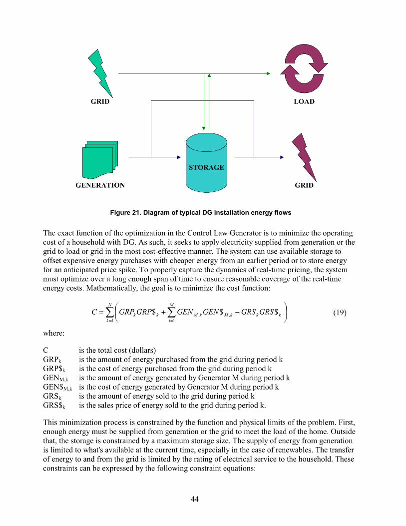
44

STORAGE

GRID

GENERATION GRID

LOAD

Figure 21. Diagram of typical DG installation energy flows

The exact function of the optimization in the Control Law Generator is to minimize the operating cost of a household with DG. As such, it seeks to apply electricity supplied from generation or the grid to load or grid in the most cost-effective manner. The system can use available storage to offset expensive energy purchases with cheaper energy from an earlier period or to store energy for an anticipated price spike. To properly capture the dynamics of real-time pricing, the system must optimize over a long enough span of time to ensure reasonable coverage of the real-time energy costs. Mathematically, the goal is to minimize the cost function:

∑ ∑= =

−+=

N

k

M

ikkkMkMkk GRSGRSGENGENGRPGRPC

1 1,, $$$ (19)

where:

C is the total cost (dollars) GRPk is the amount of energy purchased from the grid during period k GRP$k is the cost of energy purchased from the grid during period k GENM,k is the amount of energy generated by Generator M during period k GEN$M,k is the cost of energy generated by Generator M during period k GRSk is the amount of energy sold to the grid during period k GRS$k is the sales price of energy sold to the grid during period k.

This minimization process is constrained by the function and physical limits of the problem. First, enough energy must be supplied from generation or the grid to meet the load of the home. Outside that, the storage is constrained by a maximum storage size. The supply of energy from generation is limited to what's available at the current time, especially in the case of renewables. The transfer of energy to and from the grid is limited by the rating of electrical service to the household. These constraints can be expressed by the following constraint equations:

45

kkkkkk GRSLGRPGENSS −−++=+1 (20)

0SSN = (21)

MAXk LL ≤ (22)

0≥kL (23)

MAXk SS ≤ (24)

0≥kS (25)

MAXMkM GENGEN ,, ≤ (26)

0, ≥kMGEN (27)

where:

Sk, Sk+1 are the storage levels in periods k and k+1, respectively Lk is the household load during period k LMAX is the maximum possible load SMAX is the maximum amount of storage GENM,MAX is the maximum amount of generation possible from Generator M.

The structure of the constraint equations is such that all energy is routed through storage on its way to a destination. The aim is to include the energy balance, but there are many different ways that could be expressed. Given the complexity of the problem, however, this expression is more intuitively obvious than other methods. In practice, energy flows will be routed depending on the nature of the power electronics. Generation may be routed through storage to provide voltage stability, but grid-to-load energy transfers may occur directly through an AC bus. Either way, the solution provided by equations 19 through 27 will be adequate for the situation.

It should also be noted that Equation 21 sets a constraint that storage at the end of N periods should be equal to the starting storage state. This constraint is necessary to provide a bound to the entire sequence of storage states. Where the other constraints provide limits on magnitude of energy in any given period, the Equation 21 constraint provides a limit on the entire problem over N periods. The constraint applies only to storage because the energy balance equation is expressed in terms of the state of storage.

The cost (objective) function and constraint equations provide the basis for finding an optimal solution. The constraint equations confine the operating region of the system to an n-dimensional hyperspace. Within the hyperspace, every point has an associated cost in accordance with Equation 19. The goal of the optimization program is to find the single point of operation within that hyperspace that provides the lowest operating cost.

46

7.2. Solution Once the basic functionality of the system was clear, it was relatively easy to apply linear programming methods to compose a cost-minimizing objective function and appropriate constraints. Although a detailed discussion of the actual procedures used to solve the equations framed above is outside the scope of this document, it should be noted that the solution arose from recognizing and exploiting the supply/demand structure of the problem. In this manner, it was possible to greatly simplify the solution, allowing use of simpler and faster algorithms for solving the optimization problem.

Surrounding a basic optimizing engine with iterative routines for storage allocation and grid demand created a complete code capable of optimizing energy transactions over 24 hours. The code was tested and run in MATLAB on five separate cases and found to operate consistently and correctly.

7.3. Results Two straightforward scenarios that could be readily solved and verified on a spreadsheet were prepared to demonstrate the operation of the program. The Control Law Generator program was tested in these scenarios to quantify the performance of the Control Law Generator subsystem.

The basis for the scenarios is a household with 1.5 kW of photovoltaic generation and a load of approximately 21 kWh/day. On a sunny day, the photovoltaic generation provides about 14 kWh of electric energy, which is nearly enough to independently power the building. At peak generation, the power generated by the photovoltaic system exceeds the actual demand. It is assumed that a real-time pricing signal for electricity is available to the home. A price structure based on an average daily electricity rate of $0.125 and typical consumer behavior has been created for the scenario. This household does not export power to the grid but uses generation and onsite storage to offset energy purchases.

7.3.1. Case A: Sunny Day The load and generation characteristics for the house along with the utility pricing structure for a single day are shown in Figure 22.

47

0

0.2

0.4

0.6

0.8

1

1.2

1.4

1.6

1.8

1 2 3 4 5 6 7 8 9 10 11 12 13 14 15 16 17 18 19 20 21 22 23 24Hour

Ener

gy (k

Wh)

0

0.02

0.04

0.06

0.08

0.1

0.12

0.14

0.16

0.18

0.2

Elec

tric

ity P

rice

($)

LoadGenerationPrice

Figure 22. Load, generation, and utility pricing profiles for a sunny day

If this household uses no intelligent control and simply lets generation offset electricity use when available, the cost structure is that shown in Figure 23. The photovoltaic energy does a nice job of offsetting the high electricity prices that occur around mid-day but fails to mitigate the high prices later in the day. If, instead, the excess energy is stored in batteries for use at later times as is typical with battery charging systems, the household can save additional money. To keep the simulation realistic, the amount of storage available is capped at 5 kWh. The cost result of that situation is illustrated in Figure 24.

48

$-

$0.05

$0.10

$0.15

$0.20

$0.25

Cos

t ($)

1 2 3 4 5 6 7 8 9 10 11 12 13 14 15 16 17 18 19 20 21 22 23 24Hour

Total Cost: $1.3323

Figure 23. Default operating cost of a household with photovoltaic generation

$-

$0.02

$0.04

$0.06

$0.08

$0.10

$0.12

$0.14

$0.16

$0.18

$0.20

Cos

t ($)

1 2 3 4 5 6 7 8 9 10 11 12 13 14 15 16 17 18 19 20 21 22 23 24Hour

Total Cost: $0.6837

Figure 24. Operating cost of a household with photovoltaic generation and storage

49

By comparing Figure 23 and Figure 24, one can see that the ability to charge storage from generation in the middle of the day improved the household's cost performance in the evening and created savings of $0.65 (49%) over the system without storage.

Given the same system, the Control Law Generator optimizer recommends energy transactions that produce the cost structure shown in Figure 25.

$-

$0.02

$0.04

$0.06

$0.08

$0.10

$0.12

$0.14

$0.16

Cos

t ($)

1 2 3 4 5 6 7 8 9 10 11 12 13 14 15 16 17 18 19 20 21 22 23 24Hour

Total Cost: $0.5969

Figure 25. Optimal cost for household with photovoltaic generation and storage

The optimized system uses cheap electricity rates in the early morning hours to charge batteries from the grid in anticipation of needing more stored energy later in the day. The result is a savings of $0.09 (13%) over the basic charging system and $0.74 (55%) over the system without storage.

The key element to the success of the optimized system is the predictive ability that is implied in its operation. The optimization program operates on a solid knowledge of market prices and load for the entire 24-hour period it studies. In contrast, the charging system is reacting "in the moment" to available generation, load, and state of storage. This means that savings achieved through optimization reflect the overall strategy of predictive optimization that the DENNISTM system is creating. Without the predictions of generation, load, and market price, the system could not successfully store energy prior to an anticipated shortfall.

50

7.3.2. Case B: Rainy Day The simulations in Case A assumed that weather conditions were such that generation from the 1.5-kW photovoltaic unit were maximized. Case B considers the case in which a morning rainstorm gives way to a sunny afternoon. Because of the reduced insolation, the charged storage system is unable to pre-charge the batteries with photovoltaic power prior to the afternoon and evening demand increase. The total energy generated by the photovoltaic panels is just under 9 kWh. Figure 26 shows the load, generation, and price profiles for the rainy day case.

0

0.2

0.4

0.6

0.8

1

1.2

1.4

1.6

1.8

1 2 3 4 5 6 7 8 9 10 11 12 13 14 15 16 17 18 19 20 21 22 23 24Hour

Ener

gy (k

Wh)

0

0.02

0.04

0.06

0.08

0.1

0.12

0.14

0.16

0.18

0.2

Elec

trici

ty P

rice

($)

LoadGenerationPrice

Figure 26. Load, generation, and utility pricing profiles for a rainy day

As in Figure 23, where no storage is present and the available photovoltaic generation offsets current energy demand, Figure 27 shows the cost structure created by rainy day insolation levels.

The only meaningful reduction in load occurs during the 2 p.m. to 4 p.m. timeframe, when late afternoon sun is available to generate substantial electricity. About 6 hours of prime generation were unavailable to the system on this day, creating an operating cost increase of $0.28 (20%).

Using storage to capture some of the late afternoon solar energy creates some cost saving in the evening. But the storage cannot be fully charged on the limited energy available, so the system is vastly underused. The resultant cost is shown in Figure 28. One can see that the limited energy available kept the savings to a modest $0.18 (11%), much less than the $0.65 savings from a sunny day. The stored energy was applied against two high-demand hours in the evening, and that gave the homeowner some cost relief.

51

$-

$0.05

$0.10

$0.15

$0.20

$0.25

Cos

t ($)

1 2 3 4 5 6 7 8 9 10 11 12 13 14 15 16 17 18 19 20 21 22 23 24Hour

Total Cost: $1.6092

Figure 27. Default operating cost of a household with photovoltaic generation on a rainy day

$-

$0.05

$0.10

$0.15

$0.20

$0.25

Cos

t ($)

1 2 3 4 5 6 7 8 9 10 11 12 13 14 15 16 17 18 19 20 21 22 23 24Hour

Total Cost: $1.4257

Figure 28. Operating cost for household

with photovoltaic generation and storage on a rainy day

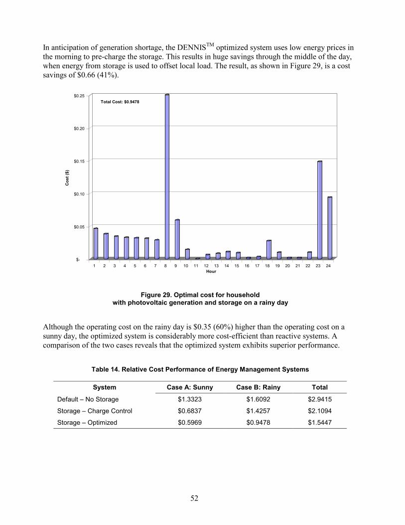
52

In anticipation of generation shortage, the DENNISTM optimized system uses low energy prices in the morning to pre-charge the storage. This results in huge savings through the middle of the day, when energy from storage is used to offset local load. The result, as shown in Figure 29, is a cost savings of $0.66 (41%).

$-

$0.05

$0.10

$0.15

$0.20

$0.25

Cos

t ($)

1 2 3 4 5 6 7 8 9 10 11 12 13 14 15 16 17 18 19 20 21 22 23 24Hour

Total Cost: $0.9478

Figure 29. Optimal cost for household with photovoltaic generation and storage on a rainy day

Although the operating cost on the rainy day is $0.35 (60%) higher than the operating cost on a sunny day, the optimized system is considerably more cost-efficient than reactive systems. A comparison of the two cases reveals that the optimized system exhibits superior performance.

Table 14. Relative Cost Performance of Energy Management Systems

System Case A: Sunny Case B: Rainy Total

Default – No Storage $1.3323 $1.6092 $2.9415

Storage – Charge Control $0.6837 $1.4257 $2.1094

Storage – Optimized $0.5969 $0.9478 $1.5447

53

7.4. Section Conclusions In this phase of the project, a mathematical description of the energy management problem and the objective of the optimizing routine were developed. A basic reclassification of the function of the Control Law Generator allowed clear definition of the inputs, outputs, and function of the module.

Once the basic functionality of the system was clear, it was relatively easy to apply linear programming methods to compose a cost-minimizing objective function and appropriate constraints. By exploiting the supply/demand structure of the problem, it was possible to greatly simplify the solution of the optimization problem by reframing the equations. This approach allowed the use of simpler and faster algorithms for solving the optimization problem.

In early benchmark comparisons of the optimized system and unoptimized systems, the Control Law Generator consistently met or beat the cost performance of the other systems. In the cases studied in this report, the Control Law Generator produced savings of $0.66 to $0.74 (41% to 55%) over a system without storage, depending on the weather. Against basic charge-controlled systems with storage, the Control Law Generator produced savings of at least 10%, with savings performance jumping to $0.48 (35%) on days with only a few hours of rain.

The focus of this task, however, was not on the absolute cost savings generated by the Control Law Generator in specific situations but on demonstrating that the optimizer operated correctly and met or exceeded the cost performance of unoptimized systems. The initial results presented here demonstrate that the optimization module is functioning as intended. Future efforts will focus on more efficient computation of the optimal energy transaction profile and provide proper interfaces to describe the generation system and associated storage.

54

8. Task 5 – Pattern Database and Pattern Recognition This section describes the development and operational results of a weather-classifying component of the Neural Pattern Database system for DENNISTM. The Neural Pattern Database applies readings from attached sensor systems to glean information about the past, present, and future operating conditions of the generator, household, and grid. The information provided by this system is used to develop an optimized control solution for dispatch of generation resources to attached load and the grid. Knowledge of weather conditions gives indications of their effect on load because of heating and cooling demands as well as future available generation from renewable resources. Knowing the amount of generation available from renewable sources lets the DENNISTM system store energy in advance of anticipated energy shortages, giving the system the ability to take advantage of real-time grid pricing by avoiding purchases or making a well-timed sale.

This section describes the pattern database work proposed in the Year One work plan. The network developed here is the foundation of the advanced network of the DENNISTM system to be tested in Year Two, which will add load, market, and other sensor readings to create an optimal control strategy for a given hour.

8.1. Background The problem of tracking weather requires unique properties that make common neural network topologies, such as backpropagation, unsuitable (see Appendix C for further information about neural network topologies). In addition to its many convergence problems, a backpropagation network will retrain and overwrite previously trained information when presented with new information that doesn’t fit learned patterns. What is needed for this application is a network that selectively learns new patterns when it can't find an appropriate match with existing patterns.

This problem is addressed directly by the ART neural networks developed by Stephen Grossberg and Gail Carpenter of Boston University. There are many varieties of ART, including ART1 for binary input patterns, ART2 for analog and binary input patterns, ART3 with a chemical reset, ARTMAP for supervised learning, and ART-EMAP for distributed learning. All of these systems are based on the basic ART block shown in Figure 30.

DENNISTM uses Fuzzy ARTMAP to process inputs to outputs. Fuzzy ARTMAP is a supervised learning network — that is, a network that is trained with known input-output pairs. Because a set of input-output pairs must be available to train the network before it provides useful classification, the network seems at odds with the DENNISTM system goal of automatic learning in the field. However, DENNISTM uses a novel feedback system that allows continuous retraining of the neural network. This constant retraining gives DENNISTM the ability to do online learning, or the ability to update the function of the neural network while it processes inputs in real time. As a result, the DENNISTM system becomes more accurate at finding optimal operating points the longer it remains in service at a given site. More complete details of the ARTMAP topology are given in Appendix C.

In all ART networks (see Figure 30), Layer F1 processes the input vector and presents it to Layer F2 through a set of weights. Based on the inner product of the F1 output and the weights, a best fit winning neuron is chosen in Layer F2. The F2 layer uses competitive feedback to select and enhance a single winning neuron while suppressing all other neurons. When F2 already contains

55

learned patterns, the F2 neuron representing the pattern that most closely resembles the input pattern is chosen. When no patterns have been learned yet, the first neuron is chosen. In the next step, the winning neuron presents its stored pattern to the Orienting Subsystem, which compares it with the input for a match. A comparison between the input pattern and the F2 pattern is made, and the result is compared against a vigilance parameter. The vigilance parameter indicates the minimum acceptable ratio between the two patterns and is always in the range 0≤ρ≤1. If the vigilance criterion is not met, Layer F2 is reset, and the previously winning neuron is suppressed until a replacement neuron can be selected. This will either represent the next closest pattern or an empty pattern. When the two patterns are adequately matched, a "resonance" condition occurs in which the stored pattern in the F2 category is made to resemble the input pattern. The speed at which this resonance transformation occurs is dependent on the programmed dynamics of the network. The change can be done either instantly or very slowly. The choice of network dynamics is totally up to the network designer. This resonance/suppression process is the key component to creating a neural network that doesn't overwrite patterns.

ρLayer F1

Layer F2

Reset

p1 p2 p3 p4

1w1,1-71w4,1-7

a1 a2 a3

2w3,1 2w3,3

2:1w3,1-4

Figure 30. ART module

For example, a summer sunny day pattern might be sufficiently different from a winter sunny day pattern that the vigilance criterion would not be met if the winter pattern were presented against the summer pattern. The ART neural network would instead seek out another category for match. Finding none, the network would create a new pattern to represent the winter sunny day.

8.2. Data Analysis ARTMAP uses supervised training to learn associations between a set of inputs and the appropriate outputs. It is imperative, therefore, to develop accurate sets of input-output pairs for training and testing. Because the function of the ARTMAP network developed here is to

56

categorize day types based on weather inputs, it was necessary to characterize available weather data and determine which day types were represented. On a given day, determining whether it is rainy or sunny is fairly easy for humans, but the process is not so obvious to machines. To help clarify information provided by the weather parameters, a clustering analysis was performed. The goal was to determine whether the data could be separated into reasonably distinct clusters for various sets of inputs. If data can be clustered in a way that generally represents different day types, then it is possible to create a neural network that will separate those clusters into output classes.

The method chosen was k-means clustering, in which the set of data points is arbitrarily divided into k clusters of data. Then, one by one, the mean of each data point is compared with the mean of each cluster to determine whether the data point is in the cluster that most closely matches its mean. The process repeats over and over until all data points are assigned to the best cluster.

Two graphical user interface (GUI)-based testing systems were developed in MATLAB to allow rapid characterization of input data. A snapshot of the 3D program in operation is shown in Figure 31. The program allows the selection of parameters and normalization levels through a pop-up screen, as shown in Figure 32. Three parameters can then be chosen to create a basic plot of the data. The lower menu areas allow the selection of an appropriate range of days and hours to test.

The GUI interfaces were used to test many combinations of input variables to find a reduced set of inputs that provided adequate clustering and characterization. Reducing the size of the input space reduces the complexity of the resulting neural network and speeds processing of data. The tradeoff comes between pre- and post-analysis of data. All data can be fed to the neural network for it to find the optimal cluster from that data, or data can be interpreted ahead of time to reduce complexity before neural processing. The latter was chosen in this case to enable an empirical understanding of the data and to select appropriate output categories for training.

Ultimately, the best clustering and prediction result from inputs of time, temperature, pressure, and insolation (normalized to approximately 1). Insolation helps predict the day type during hours when the sun is shining, but the pressure balances out the prediction in evening hours. Temperature provides another data point to complete and stabilize the information provided by other variables.

57

Figure 31. 3D clustering program in operation

58

Figure 32. Parameter selection in the 3D clustering program

Typical hourly cluster plots of these data are shown in Figure 33. The x axis (50 to 80) represents the temperature, the y axis (1,000 to 1,030) represents the barometric pressure, and the z axis (0 to 1) represents the normalized insolation. Each data point is the hourly sensor reading for one hour. An entire month of data is presented in each plot, so that the point labeled "10" is Aug. 10, 2000. The figures represent 4 a.m., 12 p.m., and 8 p.m., respectively. A different color has been assigned to each cluster so, with a glance, one can tell how well the data have been separated. They also indicate whether different hours from a single day are clustered the same. The latter test can only be applied generally, as some days have weather that changes from morning to evening. Nevertheless, the plots show that days such as August 18 are consistently clustered in a group that would probably be called "rainy."

59

Figure 33. Hourly cluster plots of weather data, plotted versus temperature (x), barometric pressure (y), and normalized insolation (z)

Top: Data for August 2000, 4 a.m.; middle: data for August 2000, 12 p.m.; bottom: data for August 2000, 8 p.m.

60

Using the clustering results with some basic adjustments from the other sensor readings, the training set shown in Figure 34 and Table 15 was developed. The two curves represent insolation (pink) and predicted output state (blue).

0.0

200.0

400.0

600.0

800.0

1000.0

1200.0

0 100 200 300 400 500 600 700

Cumulative Hour of Month

Inso

latio

n (W

/m^2

)

0.5

1.5

2.5

3.5

Day

Typ

e

Figure 34. Training and testing data for ARTMAP neural network Pink: insolation reading versus hour of the month; blue: day type training/testing point

Table 15. Partial Training Data for Neural Network

Date Time Temp Pressure Insolation 2 Hour 1 Hour Current8/1/00 1:00 63 1018.1 0 3 3 38/1/00 3:00 62.8 1017.4 0 3 3 38/1/00 6:00 62.7 1016.5 0 3 3 38/1/00 8:00 62.8 1016.1 33 3 3 38/1/00 11:00 63.1 1015.4 140 3 3 38/1/00 13:00 63.5 1014.6 226 3 3 38/1/00 16:00 64.1 1013.8 145 3 3 38/1/00 18:00 64.2 1013.2 45 3 2 28/1/00 21:00 64.3 1012.7 0 2 2 28/1/00 23:00 64.2 1013.1 0 2 2 28/2/00 2:00 62.6 1012.3 0 2 2 28/2/00 4:00 62.5 1011.6 0 2 2 28/2/00 7:00 62.4 1011.4 13 2 2 28/2/00 9:00 62.6 1011.4 124 2 2 28/2/00 12:00 63.8 1011 248 2 2 28/2/00 14:00 64.8 1010.7 208 2 2 28/2/00 17:00 66.8 1008.7 319 2 2 28/2/00 19:00 68.1 1008.1 102 2 2 28/2/00 22:00 69 1008.6 0 2 2 28/3/00 0:00 69.1 1008.6 0 2 2 18/3/00 3:00 72.3 1008.7 0 1 1 18/3/00 5:00 72.6 1008.5 0 1 1 1

TRAINING DATA

61

Three distinct output states represent rainy, hazy/partly cloudy, and sunny days. The corresponding output states are 1, 2, and 3. Table 15 contains a partial listing of the training set to demonstrate the information available for training the network. Several data points from each day are chosen to train the network. Validation of network performance is done using the remaining points. The day type for previous hours is included in the training data used as an input to the neural network. In experiments with the network, feeding back information about the past output state of the neural network helped stabilize the output so that it fluctuated less. More details of network performance will be discussed in the next section.

From Figure 34 shows that, in general, the classification of day type is related to the amount of insolation, but there are exceptions. Toward the end of the month when the sun is shining bright but the day type is indicated as hazy, the relative humidity is up around 100%. Without barometric pressure as an input, it is impossible for the ARTMAP network to accurately identify the hazy condition.

8.3. Results The network was trained with basic combinations of past and current data to decide which gave the best results. To guarantee the validity of the results, the network was trained using one set of data and tested using an entirely different set. Maintaining this separation ensures that data on the accuracy of the networks are not distorted by points from the training set and that the network will correctly classify 100% of the time.

In general, using more past hourly data stabilized the output but caused the network to gloss over temporary changes in weather. On the other hand, using only current data made the network output extremely noisy and made it difficult to extract a meaningful prediction without further processing.

Figure 35 shows the raw output using only present inputs. The plot chosen is representative of the network performance with this input set. Actual network performance varies with the order in which data are presented and with the choice of various network parameters. Each of these networks was trained with multiple random presentations of input data to minimize the effects of presentation order.

Standard output states are as follows:

Table 16. Standard Output States

State Interpretation 3 Raining 2 Hazy/Misty/Light Rain 1 Sunny 0 Not Classified

62

0

1

2

3

4

0 100 200 300 400 500 600 700

Cumulative Hour of Month

Pred

icte

d O

utpu

t Sta

teTraining Data Neural Net Prediction

Figure 35. Expected versus actual predicted output for ARTMAP neural network with only current data at input

Using only data from the present leaves significant noise in the output. The addition of past data reduces the noise in the output, but at the cost of prediction accuracy. Past data increase the probability that the network will stay in its current state and often bypass significant weather events. The output profile plotted in Figure 35 is virtually useless as is because of noise, but such noise can be filtered to produce meaningful data. By following the regions of highest plot density, it is possible to see that without the high-frequency variations, the output data will produce the correct result.

Adding a basic low-pass filter to screen out some of the noise gives a much more stable pattern. Figure 36 shows the present data-only output from Figure 35 run through a basic first-order, low-pass filter. The time constant of the filter network is five, which provides a fairly narrow passband that effectively filters off any changes that occur within a window of several hours' duration. The more gradual shifts in output state that are associated with weather trends are preserved while the random noise is filtered off.

63

0

1

2

3

4

0 100 200 300 400 500 600 700

Cumulative Hour of Month

Pred

icte

d O

utpu

t Sta

teTraining Data Neural Net Prediction

Figure 36. Filtered expected versus actual predicted output for ARTMAP neural network with only current data at input

The resulting output shows that the network is able to correctly distinguish among the three output states in most situations. This particular network showed some difficulty classifying the sunny weather around Hour 500 but eventually settled into a sunny classification. A short while later, at around hour 550, the network was right on top of a transition to hazy/misty weather.

Table 17 shows the percentage of correct answers from the neural network for filtered and unfiltered output.

Table 17. Correct Answer Percentages for Tested Networks

Network Program Raw Filtered Current plus 2 hours past data 57.40% correct 53.59% correct Current plus 1 hour past data 63.45% correct 65.92% correct Current data only 60.99% correct 78.03% correct

The best prediction accuracy achieved with any of the ARTMAP networks on this data set was around 80%. This is a very good result considering that the network was trained with a modest number of points from about a month of operation. Given the significant burden of performing clustering analysis and manually classifying large data sets, only about 1,000 data points were selected to split between training and testing. Because weather information is available several

64

times during every hour of every day, it is reasonable to expect this network to train to nearly 100% correct after a few months in service. ARTMAP networks are excellent at pattern recognition and typically exhibit correct prediction percentages in the range of 95% to 100% after only limited training.

In the DENNISTM system, the input-output data set is generated automatically from data processed at the site. As a result, the extensive data analysis that preceded the development of this piece of the network will not be necessary in the field. Further analysis of typical input sets will precede the development of the full neural network in order to determine a reduced data set for the input vector.

8.4. Section Conclusions The network developed in Year One is the foundation of the advanced network of the DENNISTM Neural Pattern Database, which will add load, market, and other sensor readings to create an optimal control strategy for a given hour. Based on the speed of training and the prediction accuracy achieved by the Fuzzy ARTMAP weather network, Orion is confident that this neural network architecture will perform extremely well in the DENNISTM system.

Using a very limited data set from about a month of weather data, the networks managed to achieve 80% accuracy in classifying the day type based on inputs of insolation, temperature, barometric pressure, and time of day. With only these simple metrics, the program was able to distinguish among rainy, hazy/rainy, and sunny days. Based on published literature on ARTMAP networks, it is entirely reasonable to expect 95% to 100% correct classification of day type with data from an additional month or two.

The development process also yielded several excellent tools that will be helpful in Year Two neural network development. The GUI-based programs for k-means clustering and data visualization will be essential for determining input data in the comprehensive system being developed in the UMLCEC laboratory.

65

9. Task 7 – Economic Analysis and Market Research/Expansion To evaluate the economic feasibility and market placement of the DENNISTM concept, Orion quantified the potential value of DENNISTM generation management technology. The focus of the investigation was the value for a residential customer with DG. The goal was to establish the economic benefit for the owner of the DG and the utility serving that customer. The analysis assumes a house with an average residential load profile and some installed generation capacity.

9.1. DENNISTM Household Controller Economics The basic operating cost of two types of generation is considered to determine the effect of generating technology on daily cost benefit. The first type of generation is solar energy collected with roof-mounted photovoltaic panels. The second is a generic hydrocarbon-based distributed generator, such as a fuel cell, microturbine, or engine genset. The concurrent evaluation of these sources gives a reasonable indication of the performance of weather-dependent versus dispatched DG. Further, in every pricing scenario, two distinct cases are considered:

1. Underproduction: the homeowner uses more power than is generated 2. Overproduction: the homeowner uses less power than is generated.

The effectiveness of the DENNISTM system is dependent on what savings can be achieved when a customer uses DR to counteract electricity consumption. The most important factor determining the savings is the monetary compensation provided to the homeowner for generated power. In the analysis that follows, several price and use scenarios are examined and related to what can be achieved using DENNISTM technology. Cost flows for the homeowner are examined under a number of electricity pricing scenarios. Energy purchases can be made at real-time or flat retail rates, and sales profit is created using avoided cost, net metering, and DENNISTM internal rates.

9.1.1. Avoided Cost Metering The avoided cost scenario uses the pricing plan mandated by the Public Utility Regulatory Policies Act (PURPA) of 1978. PURPA requires utilities to purchase generation from “qualifying facilities” (QFs) at “avoided cost.” QFs are defined in PURPA and described by related Federal Energy Regulatory Commission (FERC) rules. Generally speaking, QFs are cogenerators using fossil fuels or other small power producers using solar, wind, or geothermal energy. QFs also include projects using "alternative fuels" such as biomass, municipal wastes, or landfill gases. Avoided cost is essentially the marginal cost for a public utility to produce one more unit of power. Because QFs reduce the utility's need to produce this additional power itself, the price the utility pays for QF power has been set to this marginal cost. The utility’s avoided cost rate is determined by its state regulatory commission through a series of public hearings.

9.1.2. Net Metering Under net metering, the homeowner is compensated for power at the retail electricity rate. This provides a fantastic compensation rate for any electricity the homeowner produces and lets the consumer offset electric energy use on a 1:1 ratio with generated electricity.

Nevertheless, when the homeowner is a net exporter of energy, the compensation rate for the net difference between energy generated and energy used is only avoided cost. In practice, this means that the excellent compensation rates for the homeowner's DG disappear once he tries to become a net exporter of power.

66

9.1.3. DENNISTM Metering The DENNISTM concept uses intelligent controllers and an aggregated community to compute fair buying and selling prices for electricity. Much of the interaction of DENNISTM with the traditional utility occurs in a manner similar to that of municipal utilities or large businesses. Municipal utilities handle purchases from the grid and distribute the power to residents. Because the utility makes large purchases, it can negotiate contracts for generation and it can make special contracts. The individual customer attached to a DENNISTM community receives the dual benefit of lower electricity prices and markets for locally generated electric power.

A DENNISTM neighborhood utility acts as the aggregator for all attached DENNISTM customers. In this role, the utility purchases electricity from an outside supplier, for example, another utility, an independent generator, or the ISO. Because the DENNISTM utility is purchasing in bulk, it gets a price break. It uses the price break to create an initial cost savings that can be leveraged to create incentives for attached DG units.

In the DENNISTM system, all buy and sell transactions are cost-driven. The individual DENNISTM household controllers are designed to learn and respond to real-time market price signals. Because of this, the mechanism for getting the internal generators to buy and supply electricity at the right times is adjusting the internal electricity price over time. Energy is purchased by the home or business at the DENNISTM real-time retail rate and is sold back to the utility at the DENNISTM real-time wholesale rate. Using its adaptive intelligence, each DENNISTM unit will evaluate the historical real-time price profiles for purchases and sales and decide on the best pattern to meet the energy needs of the home or business. Further, the system will use any available storage to adjust the timing of these sales or purchases to maximize the economic benefit.

9.2. Household Controller Performance Results With the various methods by which homeowners receive value from their power management defined, the analysis proceeds to comparing all the methods. The economic performance of a household was evaluated under each of the pricing plans, and the results are summarized in Figure 37 and Figure 38. These graphs show the daily savings from discounted energy purchases (blue) and selling generation (yellow) subtracted from a base electricity cost of $2.90/day for a home with no generation. The remaining daily electricity cost is indicated by the white bar. Figure 37 shows the expected daily electricity purchases and sales for photovoltaic generation based on each type of metering. The complete analysis can be found in Appendix D.

From this side-by-side comparison, it is clear that DENNISTM offers the best price performance of all three pricing options. Although the DENNISTM photovoltaic generator does not receive as much money for generated power as it would under net metering, the electricity purchases from the DENNISTM utility are $2.35 less per day.

Figure 38 shows the same comparison for hydrocarbon-based generation. Under avoided cost or net metering, hydrocarbon-based generation shows unimpressive cost performance. However, paired with the DENNISTM system, it achieves savings of about 50%. The principal difference is in peak reduction achieved through intelligent storage and release of energy. The DENNISTM controller began storing energy early in the day prior to the energy demand peak, enabling the home to effectively pull itself off the grid in the late afternoon. Without the DENNISTM neural networks, the other methods are unable to achieve the same level of cost performance. They simply lack the ability to predict load and market parameters.

67

Avoided CostNet Metering

DENNIS(TM)

$2.16

$-

$0.74

$1.12

$-

$1.78

$0.24

$2.27

$0.39

$-

$0.50

$1.00

$1.50

$2.00

$2.50

Sales IncomePurchase SavingsDiscounted Price

Total Savings:$2.66 (92%)

Total Savings:$1.78 (61%)

Total Savings:$0.74 (26%)

Avoided CostNet Metering

DENNIS(TM)

$1.79

$-

$1.11

$0.68

$-

$2.22

$(0.67)

$2.35

$1.22

$-

$0.50

$1.00

$1.50

$2.00

$2.50

Sales IncomePurchase SavingsDiscounted Price

Total Savings:$3.57 (123%)

Total Savings:$2.22 (77%)

Total Savings:$1.11 (38%)

Figure 37. Energy purchases compared with electricity sales under various pricing plans Top: underproduction; bottom: overproduction

68

Avoided CostNet Metering

DENNIS(TM)

$2.90

$-$-

$1.90

$-

$1.00

$1.51

$1.38

$0.01

$-

$0.50

$1.00

$1.50

$2.00

$2.50

Sales IncomePurchase SavingsDiscounted Price

Total Savings:$1.39 (48%)

Total Savings:$1.00 (34%)

Total Savings:$0.00 (0%)

Avoided CostNet Metering

DENNIS(TM)

$2.90

$-$-

$1.86

$-

$1.04

$1.44

$1.37

$0.09

$-

$0.50

$1.00

$1.50

$2.00

$2.50

Sales IncomePurchase SavingsDiscounted Price

Total Savings:$1.46 (50%)

Total Savings:$1.04 (36%)

Total Savings:$0.00 (0%)

Figure 38. Electricity purchases compared with electricity sales under various pricing plans Top: underproduction; bottom: overproduction

69

9.3. Payback Period Three distinct pricing plans that describe how a home or business owner pays for generation and storage equipment have been presented. Based on the energy output levels required for overproduction in the analyses presented above, the initial investment for solar and hydrocarbon generation are assumed to be $12,500 and $5,000 respectively. This allows $5/W installed for photovoltaics and sufficient capital for generator, pad, and labor for a typical engine genset. Table 18 and Table 19 show the net present value of these investments based on a 15-year projection and 6% interest rate.

Table 18. Net Present Value of Photovoltaic Generation Investment

Initial Annual Discounted Net Present Cost Savings Savings Value

Avoided Cost 12,500 $ 405 $ $3,933 ($8,567) Net Metering 12,500 $ 810 $ $7,867 ($4,633) DENNIS 12,500 $ 1,303 $ $12,655 $155

Photovoltaic Generation

Table 19. Net Present Value of Hydrocarbon-Based Generation Investment

Initial Annual Discounted Net Present Cost Savings Savings Value

Avoided Cost 5,000 $ (372) $ ($3,613) ($8,613) Net Metering 5,000 $ 380 $ $3,691 ($1,309) DENNIS 5,000 $ 532 $ $5,167 $167

Hydrocarbon-Based Generation

9.4. Utility Revenue Potential Depending on whether the DENNISTM utility acts as an aggregator or DG dispatch coordinator, it will extract revenue either as the difference between retail and wholesale energy price or a fixed fee from the incumbent utility. In both cases, the rate is $0.05 per kilowatt-hour, on average.

To create the savings shown above, the net difference in actual energy demand to contract energy demand was approximately 3,125 kWh/day. For coordinating the dispatch and control of the attached DG, the DENNISTM utility makes $0.05/kWh x 3,125 kWh/day = $156/day, or $57,030/year. Considering that this calculation supports 258 users, we expect average annual revenue of $221/customer. In a territory with 100,000 customers, the DENNISTM utility should generate $22.1 million in revenue. This will vary with the mix of customers in the territory, the amount of peak demand, the price structure of the incumbent utility, and many other factors.

9.5. Section Conclusions The results of the benchmarking studies showed that the DENNISTM system significantly outperforms net metering and avoided cost in compensating residential DG customers for generated power. Through extensive analysis and comparison of DENNISTM with the most common compensation methods, it was concluded that DENNISTM achieves daily electricity

70

savings of 90% to 125% on a photovoltaic installation. This is 35% better performance than net metering programs and 75% better than avoided cost. A hydrocarbon installation achieves 50% savings, which is 15% better than net metering in a situation in which avoided cost cannot generate any savings.

Orion Engineering asserts that net metering is ultimately a weak method for compensating DG. Net metering fails to properly account for costs that should not be included in the price of electricity, such as utility profit, transmission fees, and regulatory charges.

By contrast, the DENNISTM system uses real-time pricing linked directly to demand to ensure fair pricing and encourage generation at proper times. Advanced control provided by the DENNISTM neural networks allows these units to learn and coordinate generation behavior in response to real demand. In most simulations, the DENNISTM controller began storing energy early in the day prior to the energy demand peak, enabling the home to effectively pull itself off the grid in the late afternoon. This was the strategic element that most improved the cost performance of the DENNISTM systems simulated in this study. Without the DENNISTM neural networks, the other methods are unable to achieve the same level of cost performance. They simply lack the ability to predict load and market parameters.

Further, the cost-based decision to remove the household from the grid greatly reduces the household's energy cost while simultaneously acting to reduce the electricity demand of the neighborhood. It is this discretionary control action, spread across all controllers in the DENNISTM territory, that enables the neighborhood utility to present a flat load profile to the incumbent utility. The result is an entirely new aggregation model supporting a variety of utility contracts.

Finally, the paybacks of hydrocarbon and photovoltaic systems were compared to evaluate the relative performance of the investments. On a photovoltaic investment of $12,500 or an investment of $5,000 on an engine genset, the DENNISTM system was able to generate a payback at a rate of return of 6% over 15 years. This compares favorably with the common payback times of 20 years or more for photovoltaics. In the process of enabling advanced distributed control of DG, the DENNISTM system makes individual DG more affordable than ever.

71

10. Conclusions At the completion of the first year of its program, Orion has accomplished all of the goals and tasks set out in its work plan. Specifically, Orion developed all the major subsystems of the DENNISTM system, upgraded facilities at UMLCEC, and developed the economics and marketing strategy for resultant products.

At the core of the work in the first year was the development of the principal subsystems for the DENNISTM household controller. The Control Law Generator was successfully designed and coded into MATLAB. Tests of the Control Law Generator in typical daily scenarios showed that it is able to extract more savings from a DG system than basic control strategies and, using the predictive abilities of the neural network, is able to create savings on days in which other systems fail outright. In the cases studied in this report, the Control Law Generator produced savings of $0.66 to $0.74 (41% to 55%) over a system without storage, depending on the weather. Against basic charge-controlled systems with storage, the Control Law Generator produced savings of at least 10%, with savings performance jumping to $0.48 (35%) on days with only a few hours of rain.

The foundations of the Neural Pattern Database were laid in place by the development of a fuzzy ARTMAP neural network to classify day types based on weather inputs. Using a very limited data set from only a month of weather data, the networks managed to achieve 80% accuracy in classifying the day type based on inputs of insolation, temperature, barometric pressure, and time of day. With only these simple metrics, the program was able to distinguish between rainy, hazy/rainy, and sunny days. Based on published literature on ARTMAP networks, it is entirely reasonable to expect 95% to 100% correct classification of day type with a small amount of additional data.

The weather-classifying neural network is the foundation of the advanced network of the DENNISTM Neural Pattern Database, which will add load, market, and other sensor readings to create an optimal control strategy for a given hour. Based on the speed of training and the prediction accuracy achieved by the Fuzzy ARTMAP weather network, Orion is confident that this neural network architecture will perform extremely well in the DENNISTM system.

In addition to these fundamental DENNISTM algorithms, Orion embarked on a series of upgrades and studies at the UMLCEC laboratories. These activities created and characterized the charge/discharge electronics needed to allow DENNISTM to control the flow of power to and from the grid and storage. Specific upgrades included:

1. Switching and power conversion devices in the laboratory had remote-operation capabilities built in, and each of these devices was tested from a central computer.

2. A 500-W PEM fuel cell was added to the existing photovoltaic and wind generation capacity installed at the laboratory.

3. A fuzzy model of the fuel cell was developed to help the DENNISTM algorithms determine fuel cost and consumption versus power output.

72

4. The harmonic content of the primary power conversion devices was measured and found to meet the intent of IEEE 519 and P1547.

5. A method for determining optimal storage sizes in DENNISTM installations was developed. These results will be used in Year Two for laboratory testing with batteries at UMLCEC and for deployment of storage at external test sites.

Each of these activities helped produce the necessary components of an integrated DENNISTM household controller. Their completion sets the stage for a transition from algorithm development to integration and testing of DENNISTM hardware and software in Year Two. Further, with complete development of the subcomponents, it was possible to do preliminary performance benchmarking of the system based on predictions of the behavior of the integrated system.

The results of the benchmarking studies showed that the DENNISTM system significantly outperforms net metering and avoided cost in compensating residential DG customers for generated power. Through extensive analysis and comparison of DENNISTM with the most common compensation methods, it was concluded that DENNISTM achieves daily electricity savings of 90% to 125% on a photovoltaic installation. This is 35% better performance than net metering programs and 75% better than avoided cost. A hydrocarbon installation achieves 50% savings, which is 15% better than net metering in a situation in which avoided cost cannot generate any savings.

In the process of developing these economic performance measures, Orion developed a working model of the DENNISTM system, including independent control at the household level and an overall integration strategy for aggregating and coordinating DG. The DENNISTM system uses real-time pricing linked directly to demand to ensure fair pricing and to encourage generation at proper times. This approach challenges programs like net metering, which include costs that should not be part of the compensation rate, such as utility profit, transmission fees, and regulatory charges.

The DENNISTM strategy of discretionary control action at the household level, spread across all controllers in the DENNISTM territory, enables the aggregated community to present a flat load profile to the incumbent utility. The end result is an entirely new aggregation model supporting a variety of utility contracts.

Once the economic return of DENNISTM had been quantified, the paybacks of hydrocarbon and photovoltaic systems were compared to evaluate the relative performance of the investments. On a photovoltaic investment of $12,500 or an investment of $5,000 on an engine genset, the DENNISTM system was able to generate a payback at a rate of return of 6% over 15 years. This compares favorably with the common payback times of 20 years or more for photovoltaics.

In the process of enabling advanced distributed control of DG, the DENNISTM system makes individual DG more affordable than ever.

A-1

Appendix A.

Figure A-1. Screen shot of wind turbine power production table

Typical fields are: VBAT battery voltage in volts XXX DCA DC current generated by each turbine or PV measured in amps XXX DCW Real power generated by each turbine or PV measured in watts INV ACA RMS AC current exported through inverter reported in amps-RMS INV W Real power exported through inverter reported in watts

A-2

Figure A-2. Screen shot of weather data table

The items reported on this table are: XXX WIND Hourly average wind measured at each turbine SUN Hourly average insolation

SKY COND Hourly observation of cloud cover. Sky condition contractions are for each layer in ascending order. Numbers following the contractions are base heights in hundreds of feet above ground level (AGL). The contractions are:

• CLR Clear below 12,000 feet • FEW 0/8–2/8 sky cover • SCT (scattered) 3/8– 4/8 sky cover • BKN (broken) 5/8–7/8 sky cover • OVC (overcast) 8/8 sky cover

VVXXX Indefinite ceiling with the vertical visibility (XXX) indicated in hundreds of feet. When clouds are composed of towering cumulus or cumulonimbus, TCU or CB (respectively) follows cloud height

VISIB Visibility in statute miles

A-3

PHENOM Weather phenomena such as tornado, funnel cloud, thunderstorm, snow, hail, haze, smoke, volcanic ash, sandstorm, squall, etc.

DRY BULB Dry bulb temperature measured in degrees Fahrenheit DEW PT Dew point temperature measured in degrees Fahrenheit WET BULB Wet bulb temperature measured in degrees Fahrenheit RH% Relative humidity percentage WIND Wind speed in knots WIND DIR Wind direction measured in tens of degrees from true north. VRB indicates variable wind with speed equal to

or less than 6 knots GUSTS Wind characteristic gusts in knots WIND CHAR Value for wind character in whole units. This item describes unusual wind characteristics such as strong gusts

(14 knots or higher) and variability (more than 60 compass degrees) PRESS Station pressure measured in inches of mercury PR TEND Pressure tendency. Assigned an integer according to the following table:

Table A-1. Pressure Tendency Codes

Primary Requirement Description

Code Figure

Increasing, then decreasing 0

Increasing, then steady, or increasing then increasing more slowly 1

Increasing steadily or unsteadily 2

Atmospheric pressure now higher than 3

hours ago Decreasing or steady, then increasing; or increasing, then increasing more rapidly 3

Increasing, then decreasing 0 Steady 4

Atmospheric pressure now same as 3 hours

ago Decreasing, then increasing 5

Decreasing, then increasing 5 Decreasing, then steady; or decreasing, then decreasing more slowly 6

Decreasing steadily or unsteadily 7

Atmospheric pressure now lower than 3 hours

ago Steady or increasing, then decreasing; or decreasing, then decreasing more rapidly 8

A-4

SL PRESS Sea level pressure PRECIP Hourly total precipitation

Figure A-3. Screen shot of ISO data table

The fields included in this table are:

SYS LOAD Electricity demand from the system during the previous 1-hour period, reported in megawatt-hours ENERGY $ Hourly marginal wholesale price for electricity bids to the energy pool, reported in dollars per megawatt-hour ENERGY STS Operational status of the energy pool TMSR $ 10-minute spinning reserve hourly marginal wholesale price, reported in dollars per megawatt-hour TMSR STS Operational status of the TMSR pool TMNSR $ 10-minute non-spinning reserve hourly marginal wholesale price, reported in dollars per megawatt-hour TMNSR STS Operational status of the TMNSR pool TMOR $ 30-minute operating reserve hourly marginal wholesale price, reported in dollars per megawatt-hour

A-5

TMOR STS Operational status of the TMOR pool AGC $ Automatic generation control hourly marginal wholesale price, reported in dollars per megawatt-hour AGC STS Operational status of the AGC pool EMER SALE Emergency electricity sales to power regions outside NE-ISO, measured in megawatt-hours EMER Emergency electricity purchases from power regions outside NE-ISO, measured in megawatt-hours

PURCH

B-1

Appendix B. The basis of fuzzy logic is the fuzzy set. The fuzzy set allows one to define degrees of truth or fitness, in contrast to the “crisp” true/false or probabilistic memberships of traditional sets. As an example, consider the task of classifying an area of ground as wet, dry, or variable (wet after heavy rainfall) based on general survey and meteorological data. A two-dimensional vector [a b] is defined to represent the description of the piece of ground, and the individual elements can assume any value between 0 and 1. For regions in which surface water is directly visible all year, it can be said with certainty that the ground is wet. In this situation, the ground-description vector might be defined as [1 0]. Similarly, one might define ground in the desert as [0 1]. For other land areas, such as a forest floor or a dry riverbed, where ground moisture differs with varying amounts of rainfall, it is more difficult to define the appropriate vector. It is this kind of situation for which fuzzy logic exists. Using traditional methods, a few options are available. The first option is to simply define a third case [1 1] or [0 0] to indicate a mixed location. Alternatively, one might opt to use probabilistic descriptions to impart some information about the probability of the ground being wet or dry at any given time. This would result in vectors such as [0.5 0.5] or [0.2 0.8] where each element represents the probability of wet or dry land. To accurately define these vectors, however, one must have a good set of observations of the ground quality over time to make a proper assignment. By contrast, fuzzy logic allows one to define the degree of truth for each element. The value of each element can be defined by a fuzzy rule that maps certain environmental conditions to membership in sets called 'wet' and 'dry', corresponding to [1 0] and [0 1] in the crisp set cases. Figure B-1 and Figure B-2 show fuzzifiers for proximity to standing water and average relative humidity of the area.

0 5 25 125 625 3125Distance from Standing Water (ft.)

0.8

0.4

0.6

0.2

WET DRY

Figure B-1. Fuzzifier for proximity to standing water

B-2

0 20 40 60 80 100Average Relative Humidity (%RH)

0.8

0.4

0.6

0.2

WETDRY

Figure B-2. Fuzzifier for average relative humidity

In an initial survey of two adjacent patches of land, it is discovered that the first patch of ground is 3 feet from a swamp and the second is 6 feet from the swamp. Using the fuzzifier in Figure B-1, the first patch of land is mapped to a wet/dry vector of [0.6 0], and the second patch is mapped to the vector [0.1 0.06]. A survey of the meteorological records of the local climate shows an average relative humidity of 70%. Based on this data and the fuzzy mapping in Figure B-2, both land patches are assigned wet/dry vectors of [0.25 0.15]. What remains now is to formulate a single two-dimensional descriptive vector from the two wet/dry vectors for each patch of ground. To do this, we enlist the aid of the fuzzy union operator. The fuzzy union operator works much like the union operator in traditional set theory. It seeks to describe the unique and overlapping area covered by two sets. The value of the fuzzy union operator is the maximum of each element in the included sets. The first patch of ground would have a fuzzy union of [0.6 0.15]. The 0.6 wet value for location-to-standing-water fuzzification is greater than the 0.25 wet value for relative humidity fuzzification. Similarly, the 0.15 dry value for relative humidity fuzzification is greater than the 0 dry value for location-to-standing-water fuzzification. The fuzzy union operation favors the factor that most directly affects the properties of the patch of ground. To demonstrate, consider two extreme cases. A patch of ground is located in the middle of a pond, but in a region with 50% RH (arid). The location-to-standing water would produce a wet value of 1, and the relative humidity would give 0. The fuzzy union operation chooses 1, which is the correct answer. Another patch of ground is in a rainforest. The ground is miles from the nearest standing water but in a region with 100% relative humidity (always raining or misting). The location-to-standing-water fuzzification gives 0, but the relative humidity gives 1. The fuzzy union result is 1, which is correct because the ground will be soggy. Applying this methodology to the two original patches of ground described above, the first patch is described by the vector [0.6 0.15], and the second is described by [0.25 0.25]. After the original fuzzification, we have two vectors representing confidence of wetness or dryness that were derived from directly measurable data. The fuzzifiers, such as those shown in Figure B-1 and Figure B-2 are developed and shaped by empirical understanding of the relationship between

B-3

wetness, dryness, and the individual parameters. The boundaries of the fuzzifier can be shifted as more data are available so that the fuzzy model becomes more refined over time. Given a group of fuzzy vectors, some additional processing may be needed to translate the fuzzy values to meaningful answers. For example, [0.6 0.15] may not be as useful as “wet,” “dry,” “probably wet,” or “65% likely to be wet.” To achieve this level of categorization, one may perform a defuzzification to convert the fuzzy input vectors to output categories. The details of that operation are omitted for brevity, but the concept is analogous to what was demonstrated in fuzzifying the patches of ground. The values of the elements in each fuzzy vector determine which output category is selected on the basis of a regional mapping. Alternatively, one can translate the fuzzy vectors into probabilities by normalizing the magnitude of the vectors to unity. For example, the probability that the ground is wet in the first patch is 80%, as calculated in Equation 28.

8.015.06.0

6.0=

+=wetP (28)

C-1

Appendix C. C.1. McCulloch-Pitts Neuron A neural network is a computational system derived from the study of biological processes. Most networks are based on simplified theoretical models of neuronal functions based on observed behavior of neuron and brain behavior in laboratory experiments. The basic building block for most neural networks is the McCulloch-Pitts neuron, developed in 1943.

Σ

inputs

p1p2p3p4

pR

b

w1

wR

n

ƒ(n)

a

neuron

Figure C-1. McCulloch-Pitts neuron with multiple inputs

(Adapted from notation of Hagan, Demuth, and Beale1)

Multiple inputs, pi, are fed into the neuron structure, and each is multiplied by a weight wi. The inputs are summed, and the result is added to a bias term, b, and fed into a transfer function that determines the appropriate output. The transfer function shown in Figure C-1 is a hard limit function for which the output is 1 if the result of the summation exceeds some threshold value and is zero otherwise. Many transfer functions are available to the designer of neural networks, and each lends unique properties to the resultant computation. The most common transfer functions are hard limit, linear, and log-sigmoid. The computation implemented by a single McCulloch-Pitts neuron, hereafter simply called a “neuron,” is:

)( bfa += Wp (29)

where: W is the vector of individual signal weights, wi [1xR]

p is the vector of input signals [Rx1]

b is the bias term (scalar)

ƒ() is the transfer function of the neuron

a is the neuron output (scalar).

1 Hagan, Martin T.; H. Demuth; M. Beale. Neural Network Design. PWS Publishing Co., Boston, 1996.

C-2

C.2. Common Neural Network Topologies The most common neural network is probably the perceptron. The perceptron and a related learning rule for training single-layer perceptron networks were proposed in a paper by Rosenblatt in 1958.2 Figure C-2 shows the topology of a multilayer perceptron neural network and outlines some of the neural network terminology.

Layer 1(Input)

Layer 2(Hidden)

Layer 3(Output)

1w1,1

1w1,2

1w2,1

1w2,2

1w3,1

1w3,2

2w1,1

2w1,2

2w1,3

2w2,1

2w2,2

2w2,3

a1

a2

a3

p1

p2

p3

Figure C-2. Typical multilayer neural network

Each AND-gate shaped symbol represents a neuron. The transfer function implemented by each neuron is depicted graphically inside the body of the neuron graphic. From the figure, one can see that the neurons in layers 1 and 2 have a linear transfer function, and the third-layer neurons have a log-sigmoid transfer function. The term “layer” refers to the ranks of neurons in the neural network. The network in Figure C-2 has three layers. The first layer in a multilayer network is usually called the input layer and is typically used to gather input signals and perform any normalization or noise cancellation that might be necessary. The last layer is the output layer because each neuron presents an element of the neural network output. In the case of a binary output signal, each neuron would represent a single bit. Any layers between the input and output layers are called hidden layers because they do not provide any direct connection to the outside of the network. Hidden layers are accorded the names 1st Hidden Layer, 2nd Hidden Layer, etc., depending on the order in which they appear from input to output. The hidden layers typically perform either a translation of the

2 F. Rosenblatt. "The Perceptron: A Probabilistic Model for Information Storage and Organization in the Brain," Psychological Review, Vol. 65, pp. 386–408, 1958.

C-3

transfer function implemented in the output layer or initial grouping of the input signals before a final grouping in the output layer. The role of the hidden layer varies widely with the type of neural network and the desired network function. A single-layer perceptron is capable of creating linear separations of the output space. This design is limited in that it is incapable of directly separating more complex regions in which the grouping is not linearly separable (see Figure C-3).

Figure C-3. Output range examples with black = 1, white = 0

Left: linearly separable with one neuron; middle: linearly separable with two neurons; right: not linearly separable with one neuron

Fortunately, adding additional layers to the perceptron readily solves this problem. This multilayer perceptron can use additional layers to assign output values to combinations of the linear separation boundaries. For example, the middle figure in Figure C-3 requires two neurons to separate the space. Each illustrated boundary marks the line at which one neuron chooses to output a 1 or a 0. Therefore, the output of a single layer network would be a 2-bit binary signal in which the output can be considered 0 for two of the four possible output states (i.e., [0 0] and [1 1]), 1 for just one of the four output states ([1 0]), and "Does Not Exist" for the last state ([0 1]). The single-layer perceptron is unable to yield a single 1 or 0 answer for a given input as in the left figure; instead, the user must interpret the 2-bit signal. By adding one more layer to translate the first-layer output into a single 1 or 0 answer, the perceptron can be built to provide a complete classification. This second layer would associate an output state of 0 with the two valid outputs from the first layer (i.e., [0 0] or [1 1] → [0]) and an output state of 1 with the remaining valid output from the first layer (i.e. [1 0] → [1]). In the examples presented thus far, the weights are assumed to be properly trained to separate the output space. The task in using multilayer perceptrons for practical purposes is to find methods for training the weights between neurons to create the appropriate transfer function that maps inputs to outputs. The backpropagation algorithm to train the weights of multilayer perceptron networks was developed in 1974 by Paul Werbos and later independently by Rumelhart, Hinton, and Williams. The fundamental process is to solve the network in the forward direction by feeding an input, computing the output, and then comparing that output to predicted output. The error is then "backpropagated" from the output layer back to the input layer. Adjustments to the individual weights in each layer are based on the product of the magnitude of the error and the sensitivity of the output to each weight. The backpropagation algorithm is intuitively simple, but most backpropagation training takes many iterations to converge to a solution. For example,

C-4

converging to a solution for a simple three-layer, seven-neuron network can take tens of thousands or even millions of iterations. The backpropagation algorithm is also very sensitive to the initial state of the network and is easily led along a path that converges to a stable local minimum where it becomes trapped so it can never find the global minimum. Many tricks have been developed to speed convergence of backpropagation networks and kick the solution out of local minima, but these networks remain stubborn for most applications. Given the simplicity of the training method, however, the backpropagation algorithm and multilayer perceptrons are very popular for neural network applications in real-world applications. C.3. ARTMAP ARTMAP stands for Adaptive Resonance Theory with MAPping. An ARTMAP network consists of two side-by-side ART modules as shown in Figure C-4. The first ART, ARTA, processes the inputs to detect categories of inputs. The second ART, ARTB, examines the set of known outputs for output categories. The expectation, or winning pattern, from each ART is compared in a Mapping Field for a match.

ρΑLayer F1A

Layer F2A

Reset

p1 p2 p3 p4

1wA1,1-7

1wA4,1-7

a1A a2

A anA

2wA3,1

2wA3,n

2:1wA3,1-4

ρΒLayer F1B

Layer F2B

Reset

a1 a2

1wB1,1-7

1wB2,1-7

a1B a2

B anB

2wB5,1

2wB5,n

2:1wB5,1-2

Inter-ARTAssociative

Memory... ...

Inter-ART Reset

ρ

Figure C-4. Block diagram of ARTMAP architecture

An input vector is applied to the ARTA network (left). The ART network processes the input and selects the appropriate category in layer F2

A based on the setting of the vigilance parameter ρA. The pattern associated with the winning F2

A category is presented to the Mapping Field, which is labeled on the diagram as Inter-ART Associative Memory. Similarly, the paired output vector associated with the input vector is applied to the input of the ARTB network (right). The ART network then determines an appropriate output category for the ARTB input. The pattern associated with the winning F2

B category is also presented to the Mapping Field.

C-5

The two patterns are then compared with each other in the Mapping Field and held up against the Inter-ART vigilance parameter, ρ. If the match between the ARTA and ARTB output vectors are suitable, then the weights between Layer F2

A and the Mapping Field are adjusted to match the pattern presented by Layer F2

B. Simultaneously, the ARTA network resonates and learns its input pattern. When the patterns at the Mapping Field do not meet the vigilance criterion, an Inter-Art Reset is issued. During the Inter-Art Reset, the vigilance parameter of the ARTA network is raised just far enough so that the winning neuron of ARTA no longer wins the competition. This causes the ARTA network to seek or create a new category in Layer F2

A. This particular feedback ensures that a new category is selected for data that doesn't fit the current pattern set. By dynamically adjusting the ARTA vigilance, the ARTMAP network ensures that there will be just enough categories created to cover all possible input-output pairs. ARTMAP also trains significantly faster than backpropagation, so it is much more practical for the task of learning patterns.

D-1

Appendix D. D.1. DENNISTM Household Controller Economics This report presents a preliminary economic analysis of a single house using DENNISTM technology. The analysis assumes a house with average residential load profile and some generation capacity installed. The type of generation source is considered in relation to the basic operating cost to determine its effect on electricity price. We assume two types of generation. The first is solar energy collected with roof-mounted photovoltaic panels. The second is a generic hydrocarbon-based distributed generator such as a fuel cell, microturbine, or engine genset. The selection of these sources gives a reasonable indication of the performance of weather-dependent versus free-running DG. The purpose of the analysis is to approximate the benefits that a single homeowner may receive from using DENNISTM technology. Specifically, it examines the cost flows for the homeowner under a number of electricity pricing scenarios. For purchases, it looks at retail purchases from the utility and retail purchases inside a DENNISTM neighborhood. For sales, it examines avoided cost, net metering, and DENNISTM internal sales. Base Case Figure D-1 shows seasonal load profiles for a typical residence. The profiles are representative days from class-average load shape data published by the Massachusetts Electric Company.

0

0.2

0.4

0.6

0.8

1

1.2

1.4

1 2 3 4 5 6 7 8 9 10 11 12 13 14 15 16 17 18 19 20 21 22 23 24

Time of Day

Ave

rage

Loa

d (k

W)

FallWinterSpringSummer

Figure D-1. Seasonal load profiles

The retail cost of electricity for this residence is based on residential rate structure R-1 (Residential General Use). The composite price per kilowatt-hour is computed in Table D-1.

D-2

Table D-1. Composite Electricity Price Based on Rate R-1

Average Monthly Usage: 575 kWh

Monthly Charges: Customer Charge $6.43/month/575 0.0112 $ /kWh Distribution Charge 0.0390 $ /kWh Transmission Charge 0.0065 $ /kWh Transition Charge 0.0156 $ /kWh Demand Side Mgmt Charge 0.0025 $ /kWh Renewables Charge 0.0008 $ /kWh

Supplier Service 0.0639 $ /kWh

0.1394 $ /kWh Composite Unit Price: To produce this unit rate, the monthly customer charge had to be unitized, but this is really a fixed cost. In the analyses that follow, the customer uses about 575 kWh per month, so the customer charge is reasonably applied. At this consumption level, the customer would pay $80.16 per month for electricity. To assess the effectiveness of the DENNISTM system, Orion is interested in what happens when this customer uses distributed resources to counteract electricity consumption. The most important consideration is the monetary value of the generated power. In the analyses that follow, several price and use scenarios are examined and related to what can be achieved using DENNISTM technology. In all cases, the concern is with the value of the homeowner’s power. D.1.1. Avoided Cost Metering Under the avoided cost scenario, the analysis considers the pricing plan mandated by PURPA in 1978. PURPA requires utilities to purchase generation from “qualifying facilities” (QFs) at “avoided cost.” QFs are defined in PURPA and described by related FERC rules. Generally speaking, QFs are cogenerators that use fossil fuels or other small power producers that use solar, wind, or geothermal energy. QFs also include projects that use "alternative fuels" such as biomass, municipal wastes, or landfill gases. Avoided cost is essentially the marginal cost for a public utility to produce one more unit of power. Because QFs reduce the utility's need to produce this additional power itself, the price the utility pays for QF power has been set to this marginal cost. The utility’s avoided cost rate is determined by state regulatory commissions through a series of public hearings. In every pricing scenario, two distinct cases must be considered: (1) the homeowner uses more power than is generated and (2) the homeowner uses less power than is generated. How the type of generation resource affects the value of generated power must also be examined.

D-3

D.1.1.1. Photovoltaic Generation The resident adds 2 kWp of photovoltaic panels to his roof to offset the residence’s daily load. The daily usage and price of electric power for the residence are listed in Table D-2.

Table D-2. Daily Usage and Price of Electric Power at Residence

Composite Electricity Rate per kWh: 0.1394$

Time of Day Load Cost Load Cost Load Cost Load Cost

1 0.54 0.08 $ 0.68 0.09$ 0.47 0.07$ 0.71 0.10 $ 2 0.5 0.07 $ 0.63 0.09$ 0.43 0.06$ 0.6 0.08 $ 3 0.46 0.06 $ 0.61 0.09$ 0.39 0.05$ 0.54 0.08 $ 4 0.44 0.06 $ 0.61 0.09$ 0.38 0.05$ 0.51 0.07 $ 5 0.47 0.07 $ 0.59 0.08$ 0.39 0.05$ 0.5 0.07 $ 6 0.53 0.07 $ 0.72 0.10$ 0.47 0.07$ 0.49 0.07 $ 7 0.63 0.09 $ 1.01 0.14$ 0.6 0.08$ 0.54 0.08 $ 8 0.69 0.10 $ 1.05 0.15$ 0.67 0.09$ 0.63 0.09 $ 9 0.77 0.11 $ 0.85 0.12$ 0.69 0.10$ 0.76 0.11 $

10 0.77 0.11 $ 0.77 0.11$ 0.71 0.10$ 0.92 0.13 $ 11 0.87 0.12 $ 0.73 0.10$ 0.76 0.11$ 0.99 0.14 $ 12 0.9 0.13 $ 0.73 0.10$ 0.65 0.09$ 1.04 0.14 $ 13 0.87 0.12 $ 0.75 0.10$ 0.64 0.09$ 1.05 0.15 $ 14 0.75 0.10 $ 0.68 0.09$ 0.65 0.09$ 0.99 0.14 $ 15 0.65 0.09 $ 0.69 0.10$ 0.66 0.09$ 0.97 0.14 $ 16 0.73 0.10 $ 0.76 0.11$ 0.69 0.10$ 0.97 0.14 $ 17 0.88 0.12 $ 0.94 0.13$ 0.76 0.11$ 1.02 0.14 $ 18 1.05 0.15 $ 1.23 0.17$ 0.84 0.12$ 1.03 0.14 $ 19 1.13 0.16 $ 1.25 0.17$ 0.92 0.13$ 1.11 0.15 $ 20 1.11 0.15 $ 1.28 0.18$ 0.92 0.13$ 1.1 0.15 $ 21 1.05 0.15 $ 1.25 0.17$ 0.99 0.14$ 1.21 0.17 $ 22 0.97 0.14 $ 1.13 0.16$ 0.97 0.14$ 1.16 0.16 $ 23 0.76 0.11 $ 0.95 0.13$ 0.79 0.11$ 1.07 0.15 $ 24 0.67 0.09 $ 0.72 0.10$ 0.59 0.08$ 0.92 0.13 $

18.19 20.61 16.03 20.83 2.54 $ 2.87$ 2.23$ 2.90 $

Average Daily Load: 18.915 kWhAverage Daily Cost: 2.64 $

Fall (11/11/98) Winter (2/9/99) Spring (04/22/99) Summer (07/19/98)

The photovoltaic panels generate throughout the day, producing electric power that can then be sold back to the utility at avoided cost. We assume here that any generation is sold to the utility and not used inside the home. The result of this generation is a credit against daily electricity costs. The savings are quantified in Table D-3. The results clearly show that the homeowner has a net payment to the utility even when he generates more than he consumes. Adding 1 kW of generation only resulted in a $0.37/day savings on electric energy and still left a net purchase of $1.79 each day. What the analysis shows is that the homeowner is unable to match the cost of electricity purchased with the sales of energy from generation. The avoided cost structure does not properly value the generation and therefore offers only a meager incentive to the homeowner.

D-4

Table D-3. Savings from Photovoltaic Generation at Avoided Cost

Composite Electricity Rate per kWh: 0.1394$ Avoided Cost Rate per kWh Generated: $0.0400

Time of Day Insolation Load Purchase Generation Sale Generation Sale

1 0 0.71 0.10$ 0.00 -$ 0.00 - $ 2 0 0.6 0.08$ 0.00 -$ 0.00 - $ 3 0 0.54 0.08$ 0.00 -$ 0.00 - $ 4 0 0.51 0.07$ 0.00 -$ 0.00 - $ 5 0 0.5 0.07$ 0.00 -$ 0.00 - $ 6 2.598371 0.49 0.07$ 0.00 -$ 0.00 - $ 7 177.1201 0.54 0.08$ 0.35 0.01$ 0.53 0.02 $ 8 394.0469 0.63 0.09$ 0.79 0.03$ 1.18 0.05 $ 9 778.2333 0.76 0.11$ 1.56 0.06$ 2.33 0.09 $

10 968.0322 0.92 0.13$ 1.94 0.08$ 2.90 0.12 $ 11 1078.37 0.99 0.14$ 2.16 0.09$ 3.24 0.13 $ 12 1117.987 1.04 0.14$ 2.24 0.09$ 3.35 0.13 $ 13 1110.269 1.05 0.15$ 2.22 0.09$ 3.33 0.13 $ 14 1038.268 0.99 0.14$ 2.08 0.08$ 3.11 0.12 $ 15 938.434 0.97 0.14$ 1.88 0.08$ 2.82 0.11 $ 16 771.9666 0.97 0.14$ 1.54 0.06$ 2.32 0.09 $ 17 465.8908 1.02 0.14$ 0.93 0.04$ 1.40 0.06 $ 18 302.1267 1.03 0.14$ 0.60 0.02$ 0.91 0.04 $ 19 100.6527 1.11 0.15$ 0.20 0.01$ 0.30 0.01 $ 20 32.25627 1.1 0.15$ 0.06 0.00$ 0.10 0.00 $ 21 0.166131 1.21 0.17$ 0.00 -$ 0.00 - $ 22 -0.077558 1.16 0.16$ 0.00 -$ 0.00 - $ 23 0 1.07 0.15$ 0.00 -$ 0.00 - $ 24 0 0.92 0.13$ 0.00 -$ 0.00 - $

20.83 18.55 27.822.90$ 0.74$ 1.11 $

Typical Daily Load: 20.83Typical Daily Purchases: 2.90$ 2.90 $ Typical Daily Sales: 0.74$ 1.11 $ Net Daily Electricity Expense: 2.16$ 1.79 $

Production – 2 kW Production – 3 kW Consumption

D.1.1.2. Hydrocarbon-Based Generation Photovoltaic generation is constrained by weather and time of day, so the case of hydrocarbon-based DG, such as microturbines or fuel cells, is also considered. These technologies permit generation throughout the day and night as long as fuel is available. The price and savings structure is different because of fuel costs. The composite natural gas price per kilowatt-hour is computed in Table D-4.

Table D-4. Composite Natural Gas Price Based on Residential Rate R-3

Average Monthly Usage: 4,170kWh

Monthly Charges: Customer Charge $6.65/month/4,170 0.00159 $ /kWh Distribution Charge 0.01195 $ /kWh Distribution Adjustment 0.00025 $ /kWh

Cost of Gas 0.01307 $ /kWh 0.02687 $ /kWh Composite Unit Price:

D-5

This assumes the same residence and cost structure from Table D-2 and Table D-3, but the generation availability and pricing have changed. Table D-5 shows an economic analysis for a natural-gas generator with 35% efficiency. This is midway between the efficiency of microturbines and fuel cells. It was chosen simply to identify a reasonable efficiency point for most hydrocarbon-based DG. The generator runs 24 hours a day but only at a level to match the output of the photovoltaic systems in the previous section. This should permit a direct comparison of operating costs and net sales of electricity.

Table D-5. Savings from Hydrocarbon-Based Generation at Avoided Cost

Composite Electricity Rate per kWh: 0.1394 $ Composite Gas Rate per kWh: 0.0269 $ Avoided Cost Rate per kWh Generated: 0.0400 $

Time of Fuel Day Price Load Purchase Generation Fuel Use Fuel Cost Sale Net Sale Generation Fuel Use Fuel Cost Sale Net Sale

1 0 0.71 0.10 $ 0.77 2.21 0.0593$ 0.03$ (0.03)$ 1.16 3.31 0.0890 $ 0.05 $ (0.04)$ 2 0 0.6 0.08 $ 0.77 2.21 0.0593$ 0.03$ (0.03)$ 1.16 3.31 0.0890 $ 0.05 $ (0.04)$ 3 0 0.54 0.08 $ 0.77 2.21 0.0593$ 0.03$ (0.03)$ 1.16 3.31 0.0890 $ 0.05 $ (0.04)$ 4 0 0.51 0.07 $ 0.77 2.21 0.0593$ 0.03$ (0.03)$ 1.16 3.31 0.0890 $ 0.05 $ (0.04)$ 5 0 0.5 0.07 $ 0.77 2.21 0.0593$ 0.03$ (0.03)$ 1.16 3.31 0.0890 $ 0.05 $ (0.04)$ 6 2.598371 0.49 0.07 $ 0.77 2.21 0.0593$ 0.03$ (0.03)$ 1.16 3.31 0.0890 $ 0.05 $ (0.04)$ 7 177.1201 0.54 0.08 $ 0.77 2.21 0.0593$ 0.03$ (0.03)$ 1.16 3.31 0.0890 $ 0.05 $ (0.04)$ 8 394.0469 0.63 0.09 $ 0.77 2.21 0.0593$ 0.03$ (0.03)$ 1.16 3.31 0.0890 $ 0.05 $ (0.04)$ 9 778.2333 0.76 0.11 $ 0.77 2.21 0.0593$ 0.03$ (0.03)$ 1.16 3.31 0.0890 $ 0.05 $ (0.04)$

10 968.0322 0.92 0.13 $ 0.77 2.21 0.0593$ 0.03$ (0.03)$ 1.16 3.31 0.0890 $ 0.05 $ (0.04)$ 11 1078.37 0.99 0.14 $ 0.77 2.21 0.0593$ 0.03$ (0.03)$ 1.16 3.31 0.0890 $ 0.05 $ (0.04)$ 12 1117.987 1.04 0.14 $ 0.77 2.21 0.0593$ 0.03$ (0.03)$ 1.16 3.31 0.0890 $ 0.05 $ (0.04)$ 13 1110.269 1.05 0.15 $ 0.77 2.21 0.0593$ 0.03$ (0.03)$ 1.16 3.31 0.0890 $ 0.05 $ (0.04)$ 14 1038.268 0.99 0.14 $ 0.77 2.21 0.0593$ 0.03$ (0.03)$ 1.16 3.31 0.0890 $ 0.05 $ (0.04)$ 15 938.434 0.97 0.14 $ 0.77 2.21 0.0593$ 0.03$ (0.03)$ 1.16 3.31 0.0890 $ 0.05 $ (0.04)$ 16 771.9666 0.97 0.14 $ 0.77 2.21 0.0593$ 0.03$ (0.03)$ 1.16 3.31 0.0890 $ 0.05 $ (0.04)$ 17 465.8908 1.02 0.14 $ 0.77 2.21 0.0593$ 0.03$ (0.03)$ 1.16 3.31 0.0890 $ 0.05 $ (0.04)$ 18 302.1267 1.03 0.14 $ 0.77 2.21 0.0593$ 0.03$ (0.03)$ 1.16 3.31 0.0890 $ 0.05 $ (0.04)$ 19 100.6527 1.11 0.15 $ 0.77 2.21 0.0593$ 0.03$ (0.03)$ 1.16 3.31 0.0890 $ 0.05 $ (0.04)$ 20 32.25627 1.1 0.15 $ 0.77 2.21 0.0593$ 0.03$ (0.03)$ 1.16 3.31 0.0890 $ 0.05 $ (0.04)$ 21 0.166131 1.21 0.17 $ 0.77 2.21 0.0593$ 0.03$ (0.03)$ 1.16 3.31 0.0890 $ 0.05 $ (0.04)$ 22 -0.077558 1.16 0.16 $ 0.77 2.21 0.0593$ 0.03$ (0.03)$ 1.16 3.31 0.0890 $ 0.05 $ (0.04)$ 23 0 1.07 0.15 $ 0.77 2.21 0.0593$ 0.03$ (0.03)$ 1.16 3.31 0.0890 $ 0.05 $ (0.04)$ 24 0 0.92 0.13 $ 0.77 2.21 0.0593$ 0.03$ (0.03)$ 1.16 3.31 0.0890 $ 0.05 $ (0.04)$

20.83 18.55 53.00 1.42$ 27.82 79.49 2.14 $ 0.74$ 1.11 $

2.90 $ (0.68)$ (1.02)$

Typical Daily Load: 20.83 Typical Daily Purchases: 2.90$ 2.90$ Typical Daily Sales: (0.68)$ (1.02)$ Net Daily Electricity Expense: 3.59$ 3.93$

Under Production Over Production Consumption

The startling result of this analysis is that hydrocarbon-based DG cannot be run to obtain a cost benefit under avoided cost metering. Running the generator costs the homeowner $0.0768 per kilowatt-hour generated. The $0.04 per kilowatt-hour avoided cost rate is insignificant against this kind of fuel cost. The DG resource only has value as a backup to utility power. D.1.1.3. Results Figure D-2 shows a comparison of electricity costs to electricity sales at avoided cost as a function of generation technology. Considering the huge gap between what the homeowner pays and what the homeowner is paid for electricity, it is clear that the homeowner is not receiving the full value of his electricity. Reducing this gap is crucial to making DG viable. The price performance of DG is improved considerably when the price field is leveled by net metering.

D-6

$(1.00)

$(0.50)

$-

$0.50

$1.00

$1.50

$2.00

$2.50

$3.00

Photovoltaic Hydrocarbon

PurchaseSell

$(1.50)

$(1.00)

$(0.50)

$-

$0.50

$1.00

$1.50

$2.00

$2.50

$3.00

Photovoltaic Hydrocarbon

PurchaseSell

Figure D-2. Energy purchases verses electricity sales under avoided cost metering

Top: underproduction; bottom: overproduction D.1.2. Net Metering Under net metering, the homeowner is compensated for power at the retail electricity rate. This, of course, is great for the homeowner because it is a fantastic rate for the electricity he produces. This lets the consumer offset electric energy usage on a 1:1 ratio with generated electricity. Assuming the same load profile and retail electricity costs as were used in Section 9, the resulting cost savings under solar and hydrocarbon-based generation are computed in Table D-6 and Table D-7.

D-7

Table D-6. Savings from Photovoltaic Generation with Net Metering

Composite Electricity Rate per kWh: 0.1394$

Time of Day Insolation Load Purchase Generation Sale Generation Sale

1 0 0.71 0.10$ 0.00 -$ 0.00 -$ 2 0 0.6 0.08$ 0.00 -$ 0.00 -$ 3 0 0.54 0.08$ 0.00 -$ 0.00 -$ 4 0 0.51 0.07$ 0.00 -$ 0.00 -$ 5 0 0.5 0.07$ 0.00 -$ 0.00 -$ 6 2.59837 0.49 0.07$ 0.00 -$ 0.00 -$ 7 177.1201 0.54 0.08$ 0.35 0.05$ 0.53 0.07$ 8 394.0469 0.63 0.09$ 0.79 0.11$ 1.18 0.16$ 9 778.2333 0.76 0.11$ 1.56 0.22$ 2.33 0.33$

10 968.0322 0.92 0.13$ 1.94 0.27$ 2.90 0.40$ 11 1078.37 0.99 0.14$ 2.16 0.30$ 3.24 0.45$ 12 1117.987 1.04 0.14$ 2.24 0.31$ 3.35 0.47$ 13 1110.269 1.05 0.15$ 2.22 0.31$ 3.33 0.46$ 14 1038.268 0.99 0.14$ 2.08 0.29$ 3.11 0.43$ 15 938.434 0.97 0.14$ 1.88 0.26$ 2.82 0.39$ 16 771.9666 0.97 0.14$ 1.54 0.22$ 2.32 0.32$ 17 465.8908 1.02 0.14$ 0.93 0.13$ 1.40 0.19$ 18 302.1267 1.03 0.14$ 0.60 0.08$ 0.91 0.13$ 19 100.6527 1.11 0.15$ 0.20 0.03$ 0.30 0.04$ 20 32.25627 1.1 0.15$ 0.06 0.01$ 0.10 0.01$ 21 0.166131 1.21 0.17$ 0.00 -$ 0.00 -$ 22 -0.077558 1.16 0.16$ 0.00 -$ 0.00 -$ 23 0 1.07 0.15$ 0.00 -$ 0.00 -$ 24 0 0.92 0.13$ 0.00 -$ 0.00 -$

20.83 18.55 27.82 2.90$ 2.59$ 3.88$

Typical Daily Load: 20.83Typical Daily Purchases: 2.90$ 2.90$ Typical Daily Sales: 2.59$ 3.88$ Net Daily Electricity Expense: 0.32$ (0.97)$

Under Production Over ProductionConsumption

D-8

Table D-7. Savings from Hydrocarbon-Based Generation With Net Metering

Composite Electricity Rate per kWh: 0.1394 $ Composite Gas Rate per kWh: 0.0269 $

Time of Fuel Day Price Load Purchase Generation Fuel Use Fuel Cost Sale Net Sale Generation Fuel Use Fuel Cost Sale Net Sale

1 0 0.71 0.10 $ 0.77 2.21 0.0593$ 0.1077$ 0.0484$ 1.16 3.31 0.0890 $ 0.1616 $ 0.0726$ 2 0 0.6 0.08 $ 0.77 2.21 0.0593$ 0.1077$ 0.0484$ 1.16 3.31 0.0890 $ 0.1616 $ 0.0726$ 3 0 0.54 0.08 $ 0.77 2.21 0.0593$ 0.1077$ 0.0484$ 1.16 3.31 0.0890 $ 0.1616 $ 0.0726$ 4 0 0.51 0.07 $ 0.77 2.21 0.0593$ 0.1077$ 0.0484$ 1.16 3.31 0.0890 $ 0.1616 $ 0.0726$ 5 0 0.5 0.07 $ 0.77 2.21 0.0593$ 0.1077$ 0.0484$ 1.16 3.31 0.0890 $ 0.1616 $ 0.0726$ 6 2.598371 0.49 0.07 $ 0.77 2.21 0.0593$ 0.1077$ 0.0484$ 1.16 3.31 0.0890 $ 0.1616 $ 0.0726$ 7 177.1201 0.54 0.08 $ 0.77 2.21 0.0593$ 0.1077$ 0.0484$ 1.16 3.31 0.0890 $ 0.1616 $ 0.0726$ 8 394.0469 0.63 0.09 $ 0.77 2.21 0.0593$ 0.1077$ 0.0484$ 1.16 3.31 0.0890 $ 0.1616 $ 0.0726$ 9 778.2333 0.76 0.11 $ 0.77 2.21 0.0593$ 0.1077$ 0.0484$ 1.16 3.31 0.0890 $ 0.1616 $ 0.0726$

10 968.0322 0.92 0.13 $ 0.77 2.21 0.0593$ 0.1077$ 0.0484$ 1.16 3.31 0.0890 $ 0.1616 $ 0.0726$ 11 1078.37 0.99 0.14 $ 0.77 2.21 0.0593$ 0.1077$ 0.0484$ 1.16 3.31 0.0890 $ 0.1616 $ 0.0726$ 12 1117.987 1.04 0.14 $ 0.77 2.21 0.0593$ 0.1077$ 0.0484$ 1.16 3.31 0.0890 $ 0.1616 $ 0.0726$ 13 1110.269 1.05 0.15 $ 0.77 2.21 0.0593$ 0.1077$ 0.0484$ 1.16 3.31 0.0890 $ 0.1616 $ 0.0726$ 14 1038.268 0.99 0.14 $ 0.77 2.21 0.0593$ 0.1077$ 0.0484$ 1.16 3.31 0.0890 $ 0.1616 $ 0.0726$ 15 938.434 0.97 0.14 $ 0.77 2.21 0.0593$ 0.1077$ 0.0484$ 1.16 3.31 0.0890 $ 0.1616 $ 0.0726$ 16 771.9666 0.97 0.14 $ 0.77 2.21 0.0593$ 0.1077$ 0.0484$ 1.16 3.31 0.0890 $ 0.1616 $ 0.0726$ 17 465.8908 1.02 0.14 $ 0.77 2.21 0.0593$ 0.1077$ 0.0484$ 1.16 3.31 0.0890 $ 0.1616 $ 0.0726$ 18 302.1267 1.03 0.14 $ 0.77 2.21 0.0593$ 0.1077$ 0.0484$ 1.16 3.31 0.0890 $ 0.1616 $ 0.0726$ 19 100.6527 1.11 0.15 $ 0.77 2.21 0.0593$ 0.1077$ 0.0484$ 1.16 3.31 0.0890 $ 0.1616 $ 0.0726$ 20 32.25627 1.1 0.15 $ 0.77 2.21 0.0593$ 0.1077$ 0.0484$ 1.16 3.31 0.0890 $ 0.1616 $ 0.0726$ 21 0.166131 1.21 0.17 $ 0.77 2.21 0.0593$ 0.1077$ 0.0484$ 1.16 3.31 0.0890 $ 0.1616 $ 0.0726$ 22 -0.077558 1.16 0.16 $ 0.77 2.21 0.0593$ 0.1077$ 0.0484$ 1.16 3.31 0.0890 $ 0.1616 $ 0.0726$ 23 0 1.07 0.15 $ 0.77 2.21 0.0593$ 0.1077$ 0.0484$ 1.16 3.31 0.0890 $ 0.1616 $ 0.0726$ 24 0 0.92 0.13 $ 0.77 2.21 0.0593$ 0.1077$ 0.0484$ 1.16 3.31 0.0890 $ 0.1616 $ 0.0726$

20.83 18.55 53.00 1.42$ 27.82 79.49 2.14 $ 2.59$ 3.88 $

2.90 $ 1.16$ 1.74$

Typical Daily Load: 20.83 Typical Daily Purchases: 2.90$ 2.90$ Typical Daily Sales: 1.16$ 1.74$ Net Daily Electricity Expense: 1.74$ 1.16$

Under Production Over Production Consumption

Net metering gives a strong return for photovoltaics but is less forgiving with hydrocarbon-based DG. The cost of fuel to run these DG resources consumes a significant amount of the profit from electricity sales. The analysis performed above ignores a crucial component of most net metering programs: the concept of Net Excess Generation (NEG). When the homeowner generates more electricity than he uses, the compensation rate drops back to avoided cost. Once again, the homeowner does not receive a reasonable value for the generation produced. To see the effect of this policy, refer to Table D-8 and Table D-9, which repeat the net metering analysis giving only avoided cost for NEG.

D-9

Table D-8. Savings from Photovoltaic Generation With Net Metering and Avoided

Cost Credit for Net Excess Generation

Composite Electricity Rate per kWh: 0.1394 $ Avoided Cost Rate per kWh Generated: 0.0400 $

Time of Day Insolation Load Purchase Generation Sale Generation Sale

1 0 0.71 0.10 $ 0.00 -$ 0.00 - $ 2 0 0.6 0.08 $ 0.00 -$ 0.00 - $ 3 0 0.54 0.08 $ 0.00 -$ 0.00 - $ 4 0 0.51 0.07 $ 0.00 -$ 0.00 - $ 5 0 0.5 0.07 $ 0.00 -$ 0.00 - $ 6 2.598371 0.49 0.07 $ 0.00 -$ 0.00 - $ 7 177.1201 0.54 0.08 $ 0.35 0.0494 $ 0.53 0.0741 $ 8 394.0469 0.63 0.09 $ 0.79 0.0941 $ 1.18 0.1099 $ 9 778.2333 0.76 0.11 $ 1.56 0.1378 $ 2.33 0.1689 $

10 968.0322 0.92 0.13 $ 1.94 0.1689 $ 2.90 0.2076 $ 11 1078.37 0.99 0.14 $ 2.16 0.1847 $ 3.24 0.2278 $ 12 1117.987 1.04 0.14 $ 2.24 0.1928 $ 3.35 0.2375 $ 13 1110.269 1.05 0.15 $ 2.22 0.1932 $ 3.33 0.2376 $ 14 1038.268 0.99 0.14 $ 2.08 0.1815 $ 3.11 0.2230 $ 15 938.434 0.97 0.14 $ 1.88 0.1715 $ 2.82 0.2090 $ 16 771.9666 0.97 0.14 $ 1.54 0.1582 $ 2.32 0.1891 $ 17 465.8908 1.02 0.14 $ 0.93 0.1299 $ 1.40 0.1573 $ 18 302.1267 1.03 0.14 $ 0.60 0.0842 $ 0.91 0.1263 $ 19 100.6527 1.11 0.15 $ 0.20 0.0281 $ 0.30 0.0421 $ 20 32.25627 1.1 0.15 $ 0.06 0.0090 $ 0.10 0.0135 $ 21 0.166131 1.21 0.17 $ 0.00 -$ 0.00 - $ 22 -0.077558 1.16 0.16 $ 0.00 -$ 0.00 - $ 23 0 1.07 0.15 $ 0.00 -$ 0.00 - $ 24 0 0.92 0.13 $ 0.00 -$ 0.00 - $

20.83 18.55 27.82 2.90 $ 1.78 $ 2.22 $

Typical Daily Load: 20.83 Typical Daily Purchases: 2.90 $ 2.90 $ Typical Daily Sales: 1.78 $ 2.22 $ Net Daily Electricity Expense: 1.12 $ 0.68 $

Under Production Over Production Consumption

D-10

Table D-9. Savings from Hydrocarbon-Based Generation with Net Metering and

Avoided Cost Credit for Net Excess Generation Composite Electricity Rate per kWh: 0.1394 $ Composite Gas Rate per kWh: 0.0269 $ Avoided Cost Rate per kWh Generated: 0.0400 $

Time of Fuel Day Price Load Purchase Generation Fuel Use Fuel Cost Sale Net Sale Generation Fuel Use Fuel Cost Sale Net Sale

1 0 0.71 0.10 $ 0.77 2.21 0.0593$ 0.1015$ 0.0422$ 1.16 3.31 0.0890 $ 0.1169 $ 0.0279$ 2 0 0.6 0.08 $ 0.77 2.21 0.0593$ 0.0906$ 0.0312$ 1.16 3.31 0.0890 $ 0.1060 $ 0.0170$ 3 0 0.54 0.08 $ 0.77 2.21 0.0593$ 0.0846$ 0.0253$ 1.16 3.31 0.0890 $ 0.1000 $ 0.0111$ 4 0 0.51 0.07 $ 0.77 2.21 0.0593$ 0.0816$ 0.0223$ 1.16 3.31 0.0890 $ 0.0971 $ 0.0081$ 5 0 0.5 0.07 $ 0.77 2.21 0.0593$ 0.0806$ 0.0213$ 1.16 3.31 0.0890 $ 0.0961 $ 0.0071$ 6 2.598371 0.49 0.07 $ 0.77 2.21 0.0593$ 0.0796$ 0.0203$ 1.16 3.31 0.0890 $ 0.0951 $ 0.0061$ 7 177.1201 0.54 0.08 $ 0.77 2.21 0.0593$ 0.0846$ 0.0253$ 1.16 3.31 0.0890 $ 0.1000 $ 0.0111$ 8 394.0469 0.63 0.09 $ 0.77 2.21 0.0593$ 0.0935$ 0.0342$ 1.16 3.31 0.0890 $ 0.1090 $ 0.0200$ 9 778.2333 0.76 0.11 $ 0.77 2.21 0.0593$ 0.1065$ 0.0471$ 1.16 3.31 0.0890 $ 0.1219 $ 0.0329$

10 968.0322 0.92 0.13 $ 0.77 2.21 0.0593$ 0.1077$ 0.0484$ 1.16 3.31 0.0890 $ 0.1378 $ 0.0488$ 11 1078.37 0.99 0.14 $ 0.77 2.21 0.0593$ 0.1077$ 0.0484$ 1.16 3.31 0.0890 $ 0.1448 $ 0.0558$ 12 1117.987 1.04 0.14 $ 0.77 2.21 0.0593$ 0.1077$ 0.0484$ 1.16 3.31 0.0890 $ 0.1497 $ 0.0608$ 13 1110.269 1.05 0.15 $ 0.77 2.21 0.0593$ 0.1077$ 0.0484$ 1.16 3.31 0.0890 $ 0.1507 $ 0.0617$ 14 1038.268 0.99 0.14 $ 0.77 2.21 0.0593$ 0.1077$ 0.0484$ 1.16 3.31 0.0890 $ 0.1448 $ 0.0558$ 15 938.434 0.97 0.14 $ 0.77 2.21 0.0593$ 0.1077$ 0.0484$ 1.16 3.31 0.0890 $ 0.1428 $ 0.0538$ 16 771.9666 0.97 0.14 $ 0.77 2.21 0.0593$ 0.1077$ 0.0484$ 1.16 3.31 0.0890 $ 0.1428 $ 0.0538$ 17 465.8908 1.02 0.14 $ 0.77 2.21 0.0593$ 0.1077$ 0.0484$ 1.16 3.31 0.0890 $ 0.1478 $ 0.0588$ 18 302.1267 1.03 0.14 $ 0.77 2.21 0.0593$ 0.1077$ 0.0484$ 1.16 3.31 0.0890 $ 0.1488 $ 0.0598$ 19 100.6527 1.11 0.15 $ 0.77 2.21 0.0593$ 0.1077$ 0.0484$ 1.16 3.31 0.0890 $ 0.1567 $ 0.0677$ 20 32.25627 1.1 0.15 $ 0.77 2.21 0.0593$ 0.1077$ 0.0484$ 1.16 3.31 0.0890 $ 0.1557 $ 0.0667$ 21 0.166131 1.21 0.17 $ 0.77 2.21 0.0593$ 0.1077$ 0.0484$ 1.16 3.31 0.0890 $ 0.1616 $ 0.0726$ 22 -0.077558 1.16 0.16 $ 0.77 2.21 0.0593$ 0.1077$ 0.0484$ 1.16 3.31 0.0890 $ 0.1616 $ 0.0726$ 23 0 1.07 0.15 $ 0.77 2.21 0.0593$ 0.1077$ 0.0484$ 1.16 3.31 0.0890 $ 0.1527 $ 0.0637$ 24 0 0.92 0.13 $ 0.77 2.21 0.0593$ 0.1077$ 0.0484$ 1.16 3.31 0.0890 $ 0.1378 $ 0.0488$

20.83 18.55 53.00 1.42$ 27.82 79.49 2.14 $ 2.42$ 3.18 $

2.90 $ 1.00$ 1.04$

Typical Daily Load: 20.83 Typical Daily Purchases: 2.90$ 2.90$ Typical Daily Sales: 1.00$ 1.04$ Net Daily Electricity Expense: 1.91$ 1.86$

Under Production Over Production Consumption

Accounting for the NEG has further reduced the benefit of using hydrocarbon-based DG and seriously diminished the benefit from the photovoltaics. Results The savings from photovoltaics and hydrocarbon-based DG are summarized in Figure D-3.

D-11

$-

$0.50

$1.00

$1.50

$2.00

$2.50

$3.00

Photovoltaic Hydrocarbon

PurchaseSell

$-

$0.50

$1.00

$1.50

$2.00

$2.50

$3.00

Photovoltaic Hydrocarbon

PurchaseSell

Figure D-3. Energy purchases compared with electricity sales under net metering with

avoided cost for net excess generation Top: underproduction; bottom: overproduction

In addition to the cost difficulties, the long-term viability of a program such as net metering must be considered. Net metering exists to encourage renewables and small generation, but it artificially imposes a market price for electricity. The economics of net metering are difficult to work out from a utility’s perspective. To illustrate, consider the components of electricity cost. They are, essentially, distribution, transmission, generation, stranded, and regulatory costs.

D-12

Generation The cost to generate electricity, including fuel, labor, capital costs, etc. Transmission The cost to transport electricity from the source of generation to the

substation, where is distributed to individual homes. Distribution The cost of lines, equipment, and maintenance to bring electricity from

the transmission lines to the point of use. Stranded The cost recovery fee paid to utilities for capital investments they made

prior to deregulation. Regulatory Costs for state and local programs such as demand-side management,

energy research, and renewable incentives.

When the homeowner generates his own power to be used nearby, should he really be compensated for every one of these charges that go into the unit price of electricity? The electrons he produces do not travel through transmission lines, and he should not really be entitled to credit for profit that the utility takes. In other words, the unit price for electricity contains the utility’s overhead and fees, and the homeowner is receiving credit for these under net metering. If NEG exceeded 50% of the load in any area, the utility would actually lose its entire profit margin. A fairer price for everyone involved would pay the homeowner for the value of his generation while including only the fees incurred in moving the power from generator to consumer. The DENNISTM system contains mechanisms to accomplish the buying and selling of power in this manner. D.1.3. DENNISTM Metering The DENNISTM concept uses intelligent controllers and an aggregated community to compute fair buying and selling prices for electricity. Much of the interaction of DENNISTM with the traditional utility occurs in a manner similar to that of municipal utilities or large businesses. Municipal utilities handle purchases from the grid and distribute the power to residents. Because the utility makes large purchases, it can negotiate contracts for generation, and it can make special contracts. The individual customer attached to a DENNISTM community receives the dual benefit of lower electricity prices and markets for locally generated electric power. D.1.3.1. Aggregate Economics Consider an aggregated DENNISTM community that presents seasonal load profiles such as that shown in Figure D-4. This figure is based on the typical distribution of power consumption for Massachusetts. The aggregated load contains 258 individual loads: 229 residential customers, 24 small businesses, and 5 medium businesses. We assume that large commercial and industrial customers will seek their own power contracts outside the DENNISTM community. The daily pricing for this load, based on General Rate G-3, is computed in Table D-10.

D-13

0

100

200

300

400

500

600

1 2 3 4 5 6 7 8 9 10 11 12 13 14 15 16 17 18 19 20 21 22 23 24

FallWinterSpringSummer

Figure D-4. Seasonal load profiles for aggregated DENNISTM community

Table D-10. Daily Pricing for Aggregated DENNISTM Community Load Hour Load (kW) Energy Cost

0 301.77 3.078$ 1 264.96 2.703$ 2 243.21 2.481$ 3 231.67 2.363$ 4 227.34 2.319$ 5 226.31 2.308$ 6 242.62 2.475$ 7 274.2 2.797$ 8 318.55 3.249$ 9 371.87 10.873$ Peak

10 402.66 11.774$ Peak11 423.56 12.385$ Peak12 430.11 12.576$ Peak13 419.16 12.256$ Peak14 416.3 12.173$ Peak15 412.51 12.062$ Peak16 423.19 12.374$ Peak17 418.01 12.223$ Peak18 429.32 12.553$ Peak19 419.96 4.284$ 20 447.02 4.560$ 21 431.46 4.401$ 22 399.03 4.070$ 23 350.8 3.578$

8525.59 165.914$

Daily Charges:Monthly Fee: 7.65$ Dist. Demand Charge: 168.14$ Transit. Demand Charge: 76.57$ Transmission Charge: 38.93$

TOTAL DAILY COST: 457.203$ Average Cost per kWh: 0.0536271

D-14

To achieve an economic benefit, the DENNISTM neighborhood utility decides to limit demand to 225 kW, as shown in Figure D-5. The neighborhood utility can create a net benefit for the DENNISTM customer and a profit for itself under a few basic scenarios. Two promising methods are discussed here.

0

50

100

150

200

250

300

350

400

450

500

1 2 3 4 5 6 7 8 9 10 11 12 13 14 15 16 17 18 19 20 21 22 23 24

Hour of Day

Load

(kW

)

Actual LoadReduced Load

Figure D-5. Change in demand presented to supplying utility

D.1.3.2. Cost Benefit Option 1: Aggregation of Load and Generation In this scenario, the DENNISTM neighborhood utility acts as the aggregator for all attached DENNISTM customers. In this role, the utility purchases electricity from an outside supplier, for example, another utility, an independent generator, or the ISO. Because the DENNISTM utility is purchasing in bulk, it gets a price break. It uses the price break to create an initial cost savings that can be leveraged to create incentives for attached DG units. In the DENNISTM system, all buy and sell transactions are cost-driven. The individual DENNISTM household controllers are designed to learn and respond to real-time market price signals. Because of this, the mechanism for getting the internal generators to buy and supply at the right times is adjusting the internal electricity price over time. D.1.3.3. Cost Benefit Option 2: Generation Dispatch Control Services In this scenario, the DENNISTM neighborhood utility supplies the service of coordinating dispatch of locally connected DG for the incumbent utility. The individual DENNISTM units are activated in the same manner as in Option 1, and the cost structure remains the same.

D-15

The DENNISTM utility is paid a monthly or annual fee by the incumbent utility to supply a flat load at the physical or virtual PCC for the neighborhood. From the incumbent utility's perspective, a flat demand profile for the connected load means that it can avoid expensive power purchases at times of extreme demand. In exchange, the incumbent utility, in effect, pays a premium for power generated inside the DENNISTM neighborhood 365 days a year. On average, over 5 to 10 years, the utility expects to pay less for power purchases as a result of improved dispatch of locally connected DG. In this configuration, the DENNISTM neighborhood becomes a tool for mitigating the risk of electric price volatility. With further penetration of renewable DG inside DENNISTM neighborhoods, the effects of fuel price volatility can also be mitigated.

D.1.3.4. Household DENNISTM Cost Performance Regardless of the role the DENNISTM utility adopts, energy is purchased by the home or business at the DENNISTM real-time retail rate and is sold back to the utility at the DENNISTM real-time wholesale rate. Using its adaptive intelligence, each DENNISTM unit will evaluate the historical real-time price profiles for purchases and sales and decide on the best pattern of purchases and sales to meet the energy needs of the home or business. Further, the system will use any available storage to adjust the timing of these sales or purchases to maximize the economic benefit. Using matched generation potential in both photovoltaics and hydrocarbon-based DG, the DENNISTM controller generates the cost profiles in Table D-11 and Table D-12. DENNISTM can plot a buy/sell strategy for the photovoltaic generator that results in a net profit to the generation owner. The DENNISTM solution for the hydrocarbon-based generation creates a significant reduction of daily electricity costs by using generation to avoid expensive purchases from the grid. Small additional cost savings were generated by selling excess energy back to the grid during peak demand.

D-16

Table D-11. Savings from Photovoltaic Generation Using DENNISTM Controller

Time of Day Insolation Load Generation Purchase Sale Generation Purchase Sale

1 0 0.71 0.00 0.0008$ -$ 0.00 0.0008 $ - $ 2 0 0.6 0.00 -$ -$ 0.00 -$ - $ 3 0 0.54 0.00 0.0023$ -$ 0.00 0.0023 $ - $ 4 0 0.51 0.00 0.0164$ -$ 0.00 0.0164 $ - $ 5 0 0.5 0.00 0.0255$ -$ 0.00 0.0295 $ - $ 6 2.598371 0.49 0.00 0.0349$ -$ 0.00 0.0208 $ - $ 7 177.1201 0.54 0.35 -$ -$ 0.53 0.0006 $ - $ 8 394.0469 0.63 0.79 -$ -$ 1.18 -$ - $ 9 778.2333 0.76 1.56 -$ -$ 2.33 -$ - $

10 968.0322 0.92 1.94 -$ -$ 2.90 -$ - $ 11 1078.37 0.99 2.16 -$ -$ 3.24 -$ - $ 12 1117.987 1.04 2.24 -$ -$ 3.35 -$ - $ 13 1110.269 1.05 2.22 -$ -$ 3.33 -$ 0.2735 $ 14 1038.268 0.99 2.08 -$ -$ 3.11 -$ - $ 15 938.434 0.97 1.88 -$ -$ 2.82 -$ - $ 16 771.9666 0.97 1.54 -$ -$ 2.32 -$ - $ 17 465.8908 1.02 0.93 0.0121$ -$ 1.40 -$ - $ 18 302.1267 1.03 0.60 0.0571$ -$ 0.91 0.0159 $ - $ 19 100.6527 1.11 0.20 0.0041$ -$ 0.30 0.0124 $ - $ 20 32.25627 1.1 0.06 0.0347$ -$ 0.10 0.0013 $ - $ 21 0.166131 1.21 0.00 0.0015$ 0.3902$ 0.00 0.0015 $ 0.5244 $ 22 -0.077558 1.16 0.00 0.0028$ -$ 0.00 0.0097 $ 0.4222 $ 23 0 1.07 0.00 0.1333$ -$ 0.00 0.1333 $ - $ 24 0 0.92 0.00 0.3035$ -$ 0.00 0.3035 $ - $

20.83 18.55 27.820.63$ 0.39$ 0.55 1.22 $

Typical Daily Load: 20.83Typical Daily Purchases: 0.63$ 0.55 $ Typical Daily Sales: 0.39$ 1.22 $ Net Daily Electricity Expense: 0.24$ (0.67) $

Over Production Under Production

D-17

Table D-12. Savings from Hydrocarbon Generation Using DENNISTM Controller

Composite Gas Rate per kWh: 0.0269 $ Time of Fuel

Day Price Load Unit Generation Fuel Use Fuel Cost Purchase Sale Generation Fuel Use Fuel Cost Purchase Sale1 0.0269 $ 0.71 0.0829 $ 0.01 0.03 0.0008$ -$ -$ 0.01 0.03 0.0008 $ - $ -$ 2 0.0269 $ 0.6 0.0671 $ 0.00 0.00 -$ -$ -$ 0.00 0.00 - $ - $ -$ 3 0.0269 $ 0.54 0.0578 $ 0.00 0.00 -$ 0.0023$ -$ 0.00 0.00 - $ 0.0023 $ -$ 4 0.0269 $ 0.51 0.0529 $ 0.00 0.00 -$ 0.0164$ -$ 0.00 0.00 - $ 0.0164 $ -$ 5 0.0269 $ 0.5 0.0510 $ 0.00 0.00 -$ 0.0270$ -$ 0.00 0.00 - $ 0.0321 $ -$ 6 0.0269 $ 0.49 0.0506 $ 0.00 0.00 -$ 0.2256$ -$ 0.00 0.00 - $ 0.2205 $ -$ 7 0.0269 $ 0.54 0.0576 $ 0.00 0.00 -$ 0.0311$ -$ 0.00 0.00 - $ 0.0311 $ -$ 8 0.0269 $ 0.63 0.0711 $ 0.00 0.00 -$ 0.0448$ -$ 0.00 0.00 - $ 0.0448 $ -$ 9 0.0269 $ 0.76 0.0901 $ 0.76 2.17 0.0583$ -$ -$ 0.06 0.17 0.0046 $ - $ -$

10 0.0269 $ 0.92 0.1130 $ 0.77 2.20 0.0591$ 0.0056$ -$ 0.02 0.06 0.0015 $ - $ -$ 11 0.0269 $ 0.99 0.1262 $ 0.77 2.20 0.0591$ 0.0025$ -$ 0.59 1.69 0.0453 $ - $ -$ 12 0.0269 $ 1.04 0.1351 $ 0.77 2.20 0.0591$ -$ 0.0026$ 1.16 3.31 0.0890 $ - $ 0.0102$ 13 0.0269 $ 1.05 0.1379 $ 0.77 2.20 0.0591$ -$ 0.0018$ 1.16 3.31 0.0890 $ - $ 0.0097$ 14 0.0269 $ 0.99 0.1332 $ 0.77 2.20 0.0591$ 0.0027$ -$ 1.16 3.31 0.0890 $ - $ 0.0142$ 15 0.0269 $ 0.97 0.1320 $ 0.77 2.20 0.0591$ -$ -$ 1.16 3.31 0.0890 $ - $ 0.0074$ 16 0.0269 $ 0.97 0.1304 $ 0.77 2.20 0.0591$ -$ -$ 1.16 3.31 0.0890 $ - $ 0.0153$ 17 0.0269 $ 1.02 0.1350 $ 0.77 2.20 0.0591$ 0.0067$ -$ 1.16 3.31 0.0890 $ - $ 0.0119$ 18 0.0269 $ 1.03 0.1327 $ 0.77 2.20 0.0591$ -$ 0.0033$ 1.16 3.31 0.0890 $ - $ 0.0108$ 19 0.0269 $ 1.11 0.1376 $ 0.77 2.20 0.0591$ 0.0041$ -$ 1.16 3.31 0.0890 $ - $ 0.0044$ 20 0.0269 $ 1.1 0.1336 $ 0.77 2.20 0.0591$ 0.0040$ -$ 1.16 3.31 0.0890 $ - $ 0.0050$ 21 0.0269 $ 1.21 0.1452 $ 0.77 2.20 0.0591$ 0.0058$ -$ 1.16 3.31 0.0890 $ - $ 0.0048$ 22 0.0269 $ 1.16 0.1385 $ 0.77 2.20 0.0591$ -$ -$ 1.16 3.31 0.0890 $ - $ -$ 23 0.0269 $ 1.07 0.1246 $ 0.77 2.20 0.0591$ -$ -$ 1.07 3.06 0.0821 $ - $ -$ 24 0.0269 $ 0.92 0.1039 $ 0.77 2.20 0.0591$ 0.1923$ -$ 0.92 2.63 0.0706 $ - $ -$

20.83 12.32 35.20 0.95$ 0.57$ 15.43 44.09 1.18 $ 0.35 $ 0.01$ 0.09$

Typical Daily Load: 20.83 20.83Typical Daily Purchases: 1.52$ 1.53$ Typical Daily Sales: 0.01$ 0.09$ Net Daily Electricity Expense: 1.51$ 1.44$

Under Production Over Production

An additional advantage of the DENNISTM community is the ability to aggregate fuel loads. The natural gas price used in these analyses assumed a gas rate based on a single residential or small-business customer. If the DENNISTM neighborhood utility makes a bulk natural gas purchase on behalf of the entire community, then the price per kilowatt-hour will drop accordingly. The DENNISTM utility might undertake this venture in the interest of encouraging generation within the community. Under the G53 – High Load Factor General Service – Large rate structure, the composite price of gas per kilowatt-hour would be that calculated in Table D-13.

Table D-13. Composite Natural Gas Price Based on Residential Rate R-3

Average Monthly Usage: 1,075,860 kWh

Monthly Charges: Customer Charge 15.10/month/1,075,860 $ 0.00001 $ /kWh Distribution Charge 0.00585 $ /kWh Distribution Adjustment (0.00010) $ /kWh

Cost of Gas 0.01307 $ /kWh 0.01884 $ /kWh Composite Unit Price:

D-18

With this price reduction, DENNISTM is able to extract additional savings of $0.28 for underproduction and $0.38 for overproduction, bringing the net daily expense to $1.23 and $1.06, respectively. D.1.3.5. Results Figure D-6 shows a comparison of energy costs to electricity sales for a single household in the DENNISTM system.

$-

$0.20

$0.40

$0.60

$0.80

$1.00

$1.20

$1.40

$1.60

Photovoltaic Hydrocarbon

PurchaseSell

$-

$0.20

$0.40

$0.60

$0.80

$1.00

$1.20

$1.40

$1.60

Photovoltaic Hydrocarbon

PurchaseSell

Figure D-6. Energy purchases compared with electricity sales via internal DENNISTM

pricing with a household controller Top: underproduction; bottom: overproduction

D-19

D.2. Utility Revenue Potential In the case presented above, the net difference between actual energy demand to contract energy demand was approximately 3,125 kWh/day. For coordinating the dispatch and control of the attached DG, the DENNISTM utility makes $0.05/kWh x 3,125 kWh/day = $156/day, or $57,030/year. Considering that this calculation supports 258 users, we expect average annual revenue of $221/customer. In a territory with 100,000 customers, the DENNISTM utility should generate $22.1 million in revenue. This number will vary with the mix of customers in the territory, the amount of peak demand, the price structure of the incumbent utility, and many other factors. D.3. Results Now that we’ve analyzed the various methods by which homeowners receive value from their generation, we compare all of the methods. Figure D-7 shows the expected daily electricity purchases and sales for photovoltaic generation based on each type of metering.

D-20

$-

$0.50

$1.00

$1.50

$2.00

$2.50

$3.00

Avoided Net Metering DENNIS

PurchaseSell

$-

$0.50

$1.00

$1.50

$2.00

$2.50

$3.00

Avoided Net Metering DENNIS

PurchaseSell

Figure D-7. Energy purchases compared with electricity sales under various pricing plans

Top: underproduction; bottom: overproduction

D-21

From this side-by-side comparison, it is clear that DENNISTM offers the best price performance of all three pricing options. Although the DENNISTM photovoltaic generator does not get as much as the same generator under net metering, the energy purchases are $2.35 less per day — a significant reduction. Figure D-8 shows the same comparison but for hydrocarbon-based generation.

$(1.50)

$(1.00)

$(0.50)

$-

$0.50

$1.00

$1.50

$2.00

$2.50

$3.00

Avoided Net Metering DENNIS

PurchaseSell

$(2.50)

$(2.00)

$(1.50)

$(1.00)

$(0.50)

$-

$0.50

$1.00

$1.50

$2.00

$2.50

$3.00

Avoided Net Metering DENNIS

PurchaseSell

Figure D-8. Electricity purchases compared with electricity sales under various pricing plans

Top: underproduction; bottom: overproduction

D-22

Hydrocarbon-based generation does not fare well under avoided cost or net metering, especially in overproduction, but does quite well in the DENNISTM system. The principal difference is in peak reduction achieved through intelligent storage and release of energy. The DENNISTM controller began storing energy early in the day in advance of the energy demand peak, enabling the home to effectively pull itself off the grid in the late afternoon. Without the solid predictions of load and market parameters by the DENNISTM neural networks, the other methods are unable to achieve the same level of cost performance. Payback Period We've examined three distinct pricing plans that describe how a home or business owner pays for generation and storage equipment. Based on the energy output levels required for overproduction in the analyses above, the initial investments for solar and hydrocarbon generation are assumed to be $12,500 and $5,000, respectively. This allows $5/W installed for photovoltaics and sufficient capital for generator, pad, and labor for a typical engine genset. Table D-14 and Table D-15 show the net present value of these investments based on a 15-year projection and 6% interest rate.

Table D-14. Net Present Value of Photovoltaic Generation Investment

Initial Annual Discounted Net Present Cost Savings Savings Value

Avoided Cost 12,500 $ 405 $ $3,933 ($8,567) Net Metering 12,500 $ 810 $ $7,867 ($4,633) DENNIS 12,500 $ 1,303 $ $12,655 $155

Photovoltaic Generation

Table D-15. Net Present Value of Hydrocarbon-Based Generation Investment

Initial Annual Discounted Net Present Cost Savings Savings Value

Avoided Cost 5,000 $ (372) $ ($3,613) ($8,613) Net Metering 5,000 $ 380 $ $3,691 ($1,309) DENNIS 5,000 $ 532 $ $5,167 $167

Hydrocarbon-Based Generation

REPORT DOCUMENTATION PAGE

Form Approved OMB NO. 0704-0188

Public reporting burden for this collection of information is estimated to average 1 hour per response, including the time for reviewing instructions, searching existing data sources, gathering and maintaining the data needed, and completing and reviewing the collection of information. Send comments regarding this burden estimate or any other aspect of this collection of information, including suggestions for reducing this burden, to Washington Headquarters Services, Directorate for Information Operations and Reports, 1215 Jefferson Davis Highway, Suite 1204, Arlington, VA 22202-4302, and to the Office of Management and Budget, Paperwork Reduction Project (0704-0188), Washington, DC 20503. 1. AGENCY USE ONLY (Leave blank)

2. REPORT DATE

June 2003

3. REPORT TYPE AND DATES COVERED

Subcontract Report

4. TITLE AND SUBTITLE Distributed Energy Neural Network Integration System: Year One Final Report

6. AUTHOR(S) T. Regan, H. Sinnock, and A. Davis

5. FUNDING NUMBERS

DP03.1001

7. PERFORMING ORGANIZATION NAME(S) AND ADDRESS(ES)

Orion Engineering Corporation University of Massachusetts Lowell PO Box 2073 One University Avenue Westford, MA 01886 Lowell, MA 01854

8. PERFORMING ORGANIZATION

REPORT NUMBER

9. SPONSORING/MONITORING AGENCY NAME(S) AND ADDRESS(ES)

National Renewable Energy Laboratory 1617 Cole Blvd. Golden, CO 80401-3393

10. SPONSORING/MONITORING

AGENCY REPORT NUMBER NREL/SR-560-34216

11. SUPPLEMENTARY NOTES

NREL Technical Monitor: Holly Thomas 12a. DISTRIBUTION/AVAILABILITY STATEMENT

National Technical Information Service U.S. Department of Commerce 5285 Port Royal Road

Springfield, VA 22161

12b. DISTRIBUTION CODE

13. ABSTRACT (Maximum 200 words) This report describes the work of Orion Engineering Corp. to develop a DER energy management module for households and small businesses and demonstrate the ability of a group of these controllers to operate through an intelligent, neighborhood controller. The controllers will provide a smart, technologically advanced, simple, efficient, and economic solution for aggregating a community of small distributed generators into a larger single, virtual generator capable of selling power or other services to a utility, independent system operator (ISO), or other entity in a coordinated manner.

15. NUMBER OF PAGES

14. SUBJECT TERMS

distributed energy neural network; DENNIS; aggregation; distributed energy; distributed power; distributed generation; National Renewable Energy Laboratory; NREL

16. PRICE CODE

17. SECURITY CLASSIFICATION

OF REPORT Unclassified

18. SECURITY CLASSIFICATION

OF THIS PAGE Unclassified

19. SECURITY CLASSIFICATION

OF ABSTRACT Unclassified

20. LIMITATION OF ABSTRACT

UL

NSN 7540-01-280-5500 Standard Form 298 (Rev. 2-89) Prescribed by ANSI Std. Z39-18 298-102