
New proximity estimate for incremental update of non uniformly distributed clusters
Upload
calin-andrei-burloiuCategory
view
55download
0description

University “Politehnica” of Bucharest
Automatic Control and Computers Faculty,Computer Science and Engineering Department
National University of Singapore
School of Computing
MASTER THESIS
Distributed Code Analysis overComputer Clusters
Scientific Advisers: Author:Prof. Khoo Siau Cheng (NUS) Călin-Andrei BurloiuProf. Nicolae T, ăpus, (UPB)
Bucharest, 2012
Universitatea “Politehnica” Bucures,ti
Facultatea de Automatică s, i Calculatoare,Catedra de Calculatoare
National University of Singapore
School of Computing
LUCRARE DE DISERTAT, IE
Analiza de cod în mod distribuitpeste clustere de calculatoare
Conducători S, tiint, ifici: Autor:Prof. Khoo Siau Cheng (NUS) Călin-Andrei BurloiuProf. Nicolae T, ăpus, (UPB)
Bucures,ti, 2012

I would like to thank my parents and my brother for their care and support. I would also liketo thank Professor Nicolae T, ăpus, for offering me the opportunity to have an internship at
National University of Singapore where I had the chance to contribute to this interesting andpromising project. Many thanks to Professor Khoo Siau Cheng for his involvement into the
project and for guiding my work to the right direction.
Abstract
This master thesis marks the first steps towards building an Internet-scale source code searchengine, forked from Sourcerer infrastructure [4]. The first part of the work is a deep analysisof the appropriateness of using a Hadoop stack for scaling up Sourcerer. The second describesthe design and implementation of the storage layer for the code analysis engine of the system,by using HBase, a distributed database for Hadoop. The third part is an implementation overHadoop MapReduce of an algorithm named Generalized CodeRank for scoring code entitiesby their popularity, as an extended application of Google’s PageRank. As far we know thisapproach is unique because it considers all entities during calculation, not only subsets ofparticular types. The results show that Generalized CodeRank gives relevant results althoughall entity types are used for computation.
Aceată lucrare de disertat, ie face primii pas, i către construirea unui motor de căutare pentru codsursă la scara Internetului, pornind de la infrastructura Sourcerer. Prima parte reprezintă oanaliză profundă a posibilităt, ii de a utiliza stiva de aplicat, ii Hadoop pentru a scala Sourcerer. Adoua parte descrie proiectarea s, i implementarea nivelului de stocare pentru motorul de analizăde cod al sistemului, folosing HBase, o bază de date distribuită pentru Hadoop. În a treiaparte este descrisă proiectarea s, i implementarea algoritmul de CodeRank generalizat pentrucalcularea scorului de popularitate a entităt, ilor de cod, ca o aplicat, ie extinsă a algoritmuluiPageRank de la Google. După cons,tint,ele mele, această abordare este unică prin faptul căinclude în calcul toate entităt, ile de code, nu doar cele de un anumit tip. Rezultatele arată căalgoritmul de CodeRank generalizat oferă rezultate relevante, în condit, iile în care entităt, i detoate tipurile sunt folosite pentru calcul.
ii

Contents
Acknowledgements i
Abstract ii
1 Introduction 11.1 Overview . . . . . . . . . . . . . . . . . . . . . . . . . . . . . . . . . . . . . . . . 21.2 Sourcerer: A Code Search and Analysis Infrastructure . . . . . . . . . . . . . . . 3
2 The Choice for Cluster Computing Technologies 52.1 Motivation . . . . . . . . . . . . . . . . . . . . . . . . . . . . . . . . . . . . . . . 52.2 MapReduce and Hadoop . . . . . . . . . . . . . . . . . . . . . . . . . . . . . . . . 6
2.2.1 MapReduce Algorithm . . . . . . . . . . . . . . . . . . . . . . . . . . . . . 62.2.2 Storage . . . . . . . . . . . . . . . . . . . . . . . . . . . . . . . . . . . . . 6
2.3 HDFS . . . . . . . . . . . . . . . . . . . . . . . . . . . . . . . . . . . . . . . . . . 62.3.1 Fault Tolerance . . . . . . . . . . . . . . . . . . . . . . . . . . . . . . . . . 72.3.2 Data Sharding . . . . . . . . . . . . . . . . . . . . . . . . . . . . . . . . . 72.3.3 High Throughput for Sequential Data Access . . . . . . . . . . . . . . . . 7
2.4 NoSQL . . . . . . . . . . . . . . . . . . . . . . . . . . . . . . . . . . . . . . . . . 72.4.1 Context . . . . . . . . . . . . . . . . . . . . . . . . . . . . . . . . . . . . . 82.4.2 Reasons . . . . . . . . . . . . . . . . . . . . . . . . . . . . . . . . . . . . . 8
2.5 HBase . . . . . . . . . . . . . . . . . . . . . . . . . . . . . . . . . . . . . . . . . . 82.5.1 Data Structuring . . . . . . . . . . . . . . . . . . . . . . . . . . . . . . . . 92.5.2 Node Roles and Data Distribution . . . . . . . . . . . . . . . . . . . . . . 92.5.3 Data Mutations . . . . . . . . . . . . . . . . . . . . . . . . . . . . . . . . . 92.5.4 Data Retrieval . . . . . . . . . . . . . . . . . . . . . . . . . . . . . . . . . 102.5.5 House Keeping . . . . . . . . . . . . . . . . . . . . . . . . . . . . . . . . . 10
2.6 The Reasons for the Chosen Technologies . . . . . . . . . . . . . . . . . . . . . . 102.6.1 Why Hadoop? . . . . . . . . . . . . . . . . . . . . . . . . . . . . . . . . . 102.6.2 ACID . . . . . . . . . . . . . . . . . . . . . . . . . . . . . . . . . . . . . . 112.6.3 CAP Theorem and PACELC . . . . . . . . . . . . . . . . . . . . . . . . . 122.6.4 SQL vs. NoSQL . . . . . . . . . . . . . . . . . . . . . . . . . . . . . . . . 13
2.7 Summary . . . . . . . . . . . . . . . . . . . . . . . . . . . . . . . . . . . . . . . . 13
3 Database Schema Design and Querying 143.1 Database Purpose . . . . . . . . . . . . . . . . . . . . . . . . . . . . . . . . . . . 143.2 Design Principles . . . . . . . . . . . . . . . . . . . . . . . . . . . . . . . . . . . . 153.3 Projects Data . . . . . . . . . . . . . . . . . . . . . . . . . . . . . . . . . . . . . . 15
3.3.1 Former SQL Database . . . . . . . . . . . . . . . . . . . . . . . . . . . . . 153.3.2 Functional Requirements . . . . . . . . . . . . . . . . . . . . . . . . . . . 163.3.3 Schema Design . . . . . . . . . . . . . . . . . . . . . . . . . . . . . . . . . 163.3.4 Querying . . . . . . . . . . . . . . . . . . . . . . . . . . . . . . . . . . . . 17
3.4 Files Data . . . . . . . . . . . . . . . . . . . . . . . . . . . . . . . . . . . . . . . . 17
iii

CONTENTS iv
3.4.1 Former SQL Database . . . . . . . . . . . . . . . . . . . . . . . . . . . . . 183.4.2 Functional Requirements . . . . . . . . . . . . . . . . . . . . . . . . . . . 183.4.3 Schema Design . . . . . . . . . . . . . . . . . . . . . . . . . . . . . . . . . 183.4.4 Querying . . . . . . . . . . . . . . . . . . . . . . . . . . . . . . . . . . . . 19
3.5 Entities Data . . . . . . . . . . . . . . . . . . . . . . . . . . . . . . . . . . . . . . 193.5.1 Former SQL Database . . . . . . . . . . . . . . . . . . . . . . . . . . . . . 193.5.2 Functional Requirements . . . . . . . . . . . . . . . . . . . . . . . . . . . 193.5.3 Schema Design . . . . . . . . . . . . . . . . . . . . . . . . . . . . . . . . . 203.5.4 Querying . . . . . . . . . . . . . . . . . . . . . . . . . . . . . . . . . . . . 22
3.6 Relations Data . . . . . . . . . . . . . . . . . . . . . . . . . . . . . . . . . . . . . 223.6.1 Former SQL Database . . . . . . . . . . . . . . . . . . . . . . . . . . . . . 223.6.2 Functional Requirements . . . . . . . . . . . . . . . . . . . . . . . . . . . 223.6.3 Schema Design . . . . . . . . . . . . . . . . . . . . . . . . . . . . . . . . . 233.6.4 Querying . . . . . . . . . . . . . . . . . . . . . . . . . . . . . . . . . . . . 24
3.7 Dangling Entities Cache . . . . . . . . . . . . . . . . . . . . . . . . . . . . . . . . 253.8 Summary . . . . . . . . . . . . . . . . . . . . . . . . . . . . . . . . . . . . . . . . 25
4 Generalized CodeRank 264.1 Reputation, PageRank and CodeRank . . . . . . . . . . . . . . . . . . . . . . . . 26
4.1.1 PageRank . . . . . . . . . . . . . . . . . . . . . . . . . . . . . . . . . . . . 264.1.2 The Random Web Surfer Behavior . . . . . . . . . . . . . . . . . . . . . . 264.1.3 CodeRank . . . . . . . . . . . . . . . . . . . . . . . . . . . . . . . . . . . . 274.1.4 The Random Code Surfer Behavior . . . . . . . . . . . . . . . . . . . . . . 28
4.2 Mathematical Model . . . . . . . . . . . . . . . . . . . . . . . . . . . . . . . . . . 284.2.1 CodeRank Basic Formula . . . . . . . . . . . . . . . . . . . . . . . . . . . 284.2.2 CodeRank Matrix Representation . . . . . . . . . . . . . . . . . . . . . . 29
4.3 Computing Generalized CodeRank with MapReduce . . . . . . . . . . . . . . . . 304.3.1 Storing Data in HBase . . . . . . . . . . . . . . . . . . . . . . . . . . . . . 304.3.2 Hadoop Jobs . . . . . . . . . . . . . . . . . . . . . . . . . . . . . . . . . . 31
4.4 Experiments . . . . . . . . . . . . . . . . . . . . . . . . . . . . . . . . . . . . . . . 324.4.1 Setup . . . . . . . . . . . . . . . . . . . . . . . . . . . . . . . . . . . . . . 324.4.2 Convergence . . . . . . . . . . . . . . . . . . . . . . . . . . . . . . . . . . 324.4.3 Probability Distribution . . . . . . . . . . . . . . . . . . . . . . . . . . . . 334.4.4 Entities CodeRank Top . . . . . . . . . . . . . . . . . . . . . . . . . . . . 344.4.5 Performance Results . . . . . . . . . . . . . . . . . . . . . . . . . . . . . . 35
5 Implementation 365.1 Database Implementation . . . . . . . . . . . . . . . . . . . . . . . . . . . . . . . 36
5.1.1 Data Modeling . . . . . . . . . . . . . . . . . . . . . . . . . . . . . . . . . 365.1.2 Database Retrieval Queries API . . . . . . . . . . . . . . . . . . . . . . . 385.1.3 Database Insertion Queries API . . . . . . . . . . . . . . . . . . . . . . . . 395.1.4 Indexing Data from Database . . . . . . . . . . . . . . . . . . . . . . . . . 40
5.2 CodeRank Implementation . . . . . . . . . . . . . . . . . . . . . . . . . . . . . . 415.2.1 CodeRank and Metrics Calculation Jobs . . . . . . . . . . . . . . . . . . . 415.2.2 Utility Jobs . . . . . . . . . . . . . . . . . . . . . . . . . . . . . . . . . . . 42
5.3 Database Querying Tools . . . . . . . . . . . . . . . . . . . . . . . . . . . . . . . 425.4 Database Utility Tools . . . . . . . . . . . . . . . . . . . . . . . . . . . . . . . . . 435.5 Database Indexing Tools . . . . . . . . . . . . . . . . . . . . . . . . . . . . . . . . 435.6 CodeRank Tools . . . . . . . . . . . . . . . . . . . . . . . . . . . . . . . . . . . . 44
6 Conclusions 466.1 Summary . . . . . . . . . . . . . . . . . . . . . . . . . . . . . . . . . . . . . . . . 466.2 Future Work . . . . . . . . . . . . . . . . . . . . . . . . . . . . . . . . . . . . . . 466.3 Related Work . . . . . . . . . . . . . . . . . . . . . . . . . . . . . . . . . . . . . . 47

CONTENTS v
A Model Types 48
B Top 100 Entities CodeRank 51
List of Figures
1.1 A Java code graph example . . . . . . . . . . . . . . . . . . . . . . . . . . . . . . 21.2 Sourcerer system architecture (as it appears in [4]) . . . . . . . . . . . . . . . . . 3
4.1 CodeRank Example . . . . . . . . . . . . . . . . . . . . . . . . . . . . . . . . . . 294.2 Variation of Euclidean distance with the growth of iteration illustrating the con-
vergence of Generalized CodeRank algorithm . . . . . . . . . . . . . . . . . . . . 334.3 Probability distribution represented by CodeRanks vector . . . . . . . . . . . . . 334.4 log-log plot for CodeRanks distribution and a power law distribution . . . . . . 344.5 Left: Top 10 Entities CodeRank chart; Right: Distribution of Top 10 Entities
CodeRanks within the whole set of entities . . . . . . . . . . . . . . . . . . . . . 35
vi

List of Tables
3.1 Columns for projects MySQL table . . . . . . . . . . . . . . . . . . . . . . . . 163.2 projects HBase Table . . . . . . . . . . . . . . . . . . . . . . . . . . . . . . . . 163.3 Columns for files MySQL table . . . . . . . . . . . . . . . . . . . . . . . . . . 183.4 files HBase Table . . . . . . . . . . . . . . . . . . . . . . . . . . . . . . . . . . 183.5 Columns for entities MySQL table . . . . . . . . . . . . . . . . . . . . . . . . 203.6 entities_hash HBase Table . . . . . . . . . . . . . . . . . . . . . . . . . . . . 213.7 entities HBase Table . . . . . . . . . . . . . . . . . . . . . . . . . . . . . . . . 213.8 Columns for relations MySQL table . . . . . . . . . . . . . . . . . . . . . . . 233.9 relations_hash HBase Table . . . . . . . . . . . . . . . . . . . . . . . . . . . 233.10 relations_direct HBase Table . . . . . . . . . . . . . . . . . . . . . . . . . . 243.11 relations_inverse HBase Table . . . . . . . . . . . . . . . . . . . . . . . . . 24
4.1 Top 10 Entities CodeRank . . . . . . . . . . . . . . . . . . . . . . . . . . . . . . . 344.2 Experiments and jobs running time . . . . . . . . . . . . . . . . . . . . . . . . . . 35
5.1 Common CLI arguments for Hadoop tools (CodeRank and Database indexingtools) . . . . . . . . . . . . . . . . . . . . . . . . . . . . . . . . . . . . . . . . . . 44
5.2 Common CLI arguments for CodeRankCalculator tool . . . . . . . . . . . . . . . 455.3 Common CLI arguments for CodeRankUtil tool . . . . . . . . . . . . . . . . . . . 45
A.1 Project Types . . . . . . . . . . . . . . . . . . . . . . . . . . . . . . . . . . . . . . 48A.2 File Types . . . . . . . . . . . . . . . . . . . . . . . . . . . . . . . . . . . . . . . . 48A.3 Entity Types . . . . . . . . . . . . . . . . . . . . . . . . . . . . . . . . . . . . . . 49A.4 Relation Types . . . . . . . . . . . . . . . . . . . . . . . . . . . . . . . . . . . . . 50A.5 Relation Classes . . . . . . . . . . . . . . . . . . . . . . . . . . . . . . . . . . . . 50
B.1 Top 100 Entities CodeRank (No. 1-33) . . . . . . . . . . . . . . . . . . . . . . . . 51B.2 Top 100 Entities CodeRank (No. 34-67) . . . . . . . . . . . . . . . . . . . . . . . 52B.3 Top 100 Entities CodeRank (No. 68-100) . . . . . . . . . . . . . . . . . . . . . . 53
vii

Chapter 1
Introduction
This work marks the first steps into the project “Semantic-based Code Search” initiated atUniversity of Singapore, School of Computing by Professor Khoo Siau Cheng. Its main objectiveis building a Internet-scale search engine for source code. The implementation is a fork ofSourcerer [11], a code search platform developed at University California of Irvine. My workconcentrates on putting the foundation of a code search and analysis platform by scaling upSourcerer to Internet-scale. My contribution can be divided into three parts. The first part isa deep analysis of the appropriateness of using a Hadoop stack for scaling up Sourcerer. Thesecond describes the design and implementation of the storage layer for the code analysis engine,by using HBase, a distributed database for Hadoop. And the third part is an implementationover Hadoop MapReduce of an algorithm for ranking code entities by their popularity, as anextended application of Google’s PageRank.
In the last years we assist to an increase of popularity of open-source and free software. Itmay be possible that the Web had a big impact on this by allowing everyone to share contentwith others. To make this more accessible to people, web hosting services offered access to freetechnologies like LAMP1 stack. By having a lot of users, the open-source communities becamemotivated to developed better and better software.
The expansion of open-source software also had an impact on IT business. A lot of companieslike Google, Yahoo!, Cloudera, DataStax and MapR are financing open-source projects at theexchange of payed support and premium services. On the other side of the business field, moreand more companies are starting to adopt open-source projects, technologies and libraries intotheir products not only because are free, but also because of the big communities around themwhich are able to offer good support.
The open-source movement also changed the way software architects and developers work.They need to reserve a lot of time to find libraries or technologies capable of accomplishing aparticular task or to figure out how to use them. In this context a search engine provides agood way to start by finding pieces of code, documentation, code examples or to download thesource code. During development with open-source technologies, programmers often encounterissues and searching the Web for similar problems with the purpose of finding code snippets,code examples and solutions is often part of the development phase.
Currently Google dominates the market of mainstream search engines [53]. Developers often usethis kind of search engines to download code, to find code snippets, examples and to solve theirissues, although they are not adapted for this purpose. For better results a dedicated sourcecode search engines would be more appropriate. But searching for code that is capable toaccomplish a particular task is not easy. Others tried to implement code search engines, like
1Linux, Apache, MySQL, PHP
1

CHAPTER 1. INTRODUCTION 2
the commercial solutions Koders [48], Krugle [49], Codase [14] and Google Code Search. Thefact that none of them is very popular and that users prefer to use mainstream search enginesproves the fact that state of the art code search does not satisfy users’ needs. Google CodeSearch has been shut down in 2012 most likely because of the unsolved challenges in this field.
1.1 Overview
When we started working at the “Semantic-based Code Search” project we wanted to incorporatebasic state of the art code search techniques without the need to reinvent the wheel. So wesearched for an open-source code search platform that we could extend by building our ownalgorithms on top of it. After analyzing multiple alternatives we stopped at Sourcerer [4].
One of the first reasons to choose it was that fact that as our system it aimed at an Internet-scalesearch engine. Secondly, it had the basic information retrieval techniques already implemented.The important thing was that it included a MySQL [61] database with information extractedfrom code which can be used as a basis for a lot of code analysis tools and algorithms. Sourcereronly handles Java code. We named our Sourcerer fork [11] Distributed Sourcerer because itruns on a cluster of computers, a set of tightly coupled commodity hardware computers whichwork together to a common task.
After getting deep into Sourcerer by studying its architecture and source code, as well as bytesting it, we soon realized that it would not scale to Internet size as its authors aimed, as itwill be discussed in the next section. The basic idea was that each of its components could onlyrun on a single machine. So I started to redesign it to run on a computer cluster.
My area of investigation is the code analysis part of Sourcerer infrastructure, which providesalgorithms vital to a code search engine, such as code indexing techniques, ranking of codeentities, code clone detection and code clustering.
The code analysis field investigates the structure and the semantics of program code andit is part of program analysis field which focuses on behavior. Code analysis algorithm canbe classified as compile based and non-compile based, depending on their need to compile thesource code before performing analysis or not. Non-compile based algorithms are generallyfaster because they perform static code analysis and can cope with code that contains errors,which is not compilable because of this reason. The main disadvantage of this algorithms is thatthey cannot analyze dynamically loaded code entities, like Java classes loaded during runtime.Compile-based code analysis algorithms do not have this disadvantage, but are generally slower.
Figure 1.1: A Java code graph example
Code analysis usually deals with code graphs, like the one presented in Figure 1.1. Their nodesare code entities like classes, methods, primitives and variables and their edges are relations

CHAPTER 1. INTRODUCTION 3
like “returns” in “method returns primitive” (see Figure 1.1). When a code graph only containsmethod nodes and “calls” relations it is called call graph. In a similar way graphs that onlycatch the class inheritance hierarchy or class connections can be constructed. More detailsabout entities and relations can be found in Section 3.1. A full list of all entity types andrelation types as well as an explanation of them can be found in Appendix A.
When talking about big scale systems, the data takes an important role because of its size anddifficulties to access it. A recent solution for large scale data processing is Hadoop platform [24],an open-source implementation of Google’s MapReduce programming paradigm [15]. Chapter 2presents the investigations of using this platform, as well as the reasons we decided to port theMySQL [61] database to a Hadoop-compliant database named HBase [25]. The design schemaof the new database, the reasons behind it and the techniques used to implement queries to itare explained in Chapter 3.
After porting the storage layer of the system to HBase, I implemented a ranking algorithmfor the search engine (see Chapter 4), named Generalized CodeRank, which is a PageRank[63] adaption for code analysis used for calculating entities popularity. Other state of the artworks implemented CodeRank before [64][51][55], but our approach differs from theirs by thefact that we applied the algorithm to all entities and relations from the database. Portfolio [55]only applies it to C functions and their call relations. Puppin et al. [64] apply it only to classes.As far as we know, an older version of Sourcerer [51] only applied it to several types of entities,but not simultaneously.
1.2 Sourcerer: A Code Search and Analysis Infrastructure
Developed at University California of Irvine mostly by S. Bajracharya, J. Ossher and C. Lopes,Sourcerer is a code search infrastructure which aims to grow to Internet-scale.
Figure 1.2: Sourcerer system architecture (as it appears in [4])
A crawler downloads source code found on the Internet in various repositories and stores thedata in three different forms:

CHAPTER 1. INTRODUCTION 4
1. In the Managed Repository (referred from now as repository) which keeps the originalcode and additional libraries.
2. In the Code Database named SourcererDB [62] which stores data as a metamodelobtained by parsing the code from the repository (details in Chapter 3).
3. In the Code Index which is an inverted index for keywords extracted from the code.
The system architecture is illustrated in Figure 1.2. At its core, Sourcerer applies basic informa-tion retrieval techniques to index tokenized source code into the Code Index implemented withApache Lucene [26], an open-source search engine library. To hide the complexity of Lucene, ahigher level technology is used, that is Apache Solr [29], a search server.
In 2010, Sourcerer team published a paper [5] which proposed an innovative way to efficientlyretrieve code examples. Their technique associates keywords to source code entities that havesimilar API usage. This similarity is obtained from the Code Database and the keywordsassociated are stored in the Code Index. The Code Database is a relational MySQL [61]database, which stores metamodels of projects, files, entities and relations into tables. Moreabout this in Chapter 3.
The data obtained by the crawler from the web is first stored in the Managed Repository. Inorder to populate the Code Database and the Code Index the extractor is used, which isimplemented as a headless Eclipse [37] plugin. This component is able to parse the source codeand obtain code entities and code relations data.
An older version of Sourcerer [51] implemented CodeRank, the PageRank-like algorithm forranking code entities, but the current version does not implement this any more.
Chapter 2 will talk more about the limitations of Sourcerer with respect to scalability andwill propose changing the database with a distributed one called SourcererDDB (SourcererDistributed Database). Chapter 3 will describe in detail the schema design of the new databaseand Chapter 4 will present Generalized CodeRank algorithm which runs on SourcererDDB’sdata.

Chapter 2
The Choice for Cluster ComputingTechnologies
This chapter presents the cluster computing technologies used for scaling up Sourcerer and thereason they were chosen instead of considering other alternatives.
2.1 Motivation
Chapter 1.2 described Sourcerer an open-source project from which our implementation started.Although its goals of building a large-scale system match our goals we soon realized the limi-tations regarding Sourcerer scalability:
1. SourcererDB (Sourcerer database), which uses MySQL, showed poor performance forrepositories of hundreds of gigabytes and for difficult queries required by some applica-tions.
2. The extractor, implemented as an Eclipse [37] headless plugin, can only run on a singlemachine and parsing hundreds of gigabytes takes days.
3. The real time code search application uses Apache Solr [29], a search server based onApache Lucene [26] search library. Solr runs on a single machine mode so it’s not capableto scale. There is a multi-machine version, called Distributed Solr, but currently lackssome of the Solr features. Other Lucene-based search servers like ElasticSearch [18] shouldbe investigated in the future.
Our basic idea is to port Sourcerer for technologies capable of running in a distributed manneron a computer cluster. This master thesis deals only with the first point above, by investigatingsolutions to scale the database and by designing and implementing a new distributed databasecalled SourcererDDB (Sourcerer Distributed Database), capable of scaling to thousands ofmachines and to deal with petabytes of data. The database design schema for storing code datais presented in Chapter 3 and an algorithm, Generalized CodeRank, implemented on top of itis presented in Chapter 4.
The next three sections present the technologies we chose for running our data on a computercluster. We are using HBase [25], a large-scale distributed database, and Hadoop [24], a platformfor running distributed computing computation based on MapReduce programming model [15].These technologies are capable of scaling linearly and horizontally on commodity hardware.
5

CHAPTER 2. THE CHOICE FOR CLUSTER COMPUTINGTECHNOLOGIES 6
2.2 MapReduce and Hadoop
Hadoop [24] is an open-source framework for running distributed applications developed byApache Software Foundation [28]. Its implementation is based on two Google papers, oneabout MapReduce [15] and the other about Google File System [39]. For the later the Hadoophomologous implementation is named HDFS and is described in Section 2.3, while the formerwill be detailed in this section. By the time of writing this thesis, Hadoop is very popular andwidely used in the industry by important companies like Facebook, Yahoo!, Twitter, IBM andAmazon.[35] For example, a news published on gigaom.com states that Facebook has a 100 GiBHadoop cluster [41].
MapReduce [15] is a programming model and framework which can be used to solve embarrass-ingly parallel problems consisting of very large amounts of data distributed across a cluster ofcomputers.
2.2.1 MapReduce Algorithm
MapReduce problem solving model involves two main functions, map and reduce, inspiredfrom functional programming. The execution of map functions is supervised by Map tasks andthe execution of reduce functions by Reduce tasks. From a distributed system point of view,there is a master node which coordinates jobs, and multiple slave nodes which execute tasks.The master is responsible with job scheduling by assigning tasks to slave nodes, coordinatingslaves activity and monitoring. The domain and range of the map and reduce functions arevalues structured as (key, value) pairs.[15][72]
In Hadoop, the input data is passed to an InputFormat class implementation which splits thedata into multiple parts. The master assigns a split to each slave which uses a RecordReaderto parse the input data split into input (key, value) pairs. During the map stage, each mapfunction will receive a pair and by processing it will output a set of intermediate (key, value)pairs. After the completion of all Map tasks from the whole cluster the map stage is finished.During sort and shuffling stage the master schedules the allocation of intermediate (key,values) to Reduce tasks. During reduce stage, each reduce function will receive as input aset of intermediate (key, value) pairs having the same key and through processing will outputa set of output (key, value) pairs.[15][72]
2.2.2 Storage
Hadoop stores input and output data into a distributed file system or in a distributed database[72]. It comes with its own distributed file system implementation, which is HDFS, but otherimplementation ca be used. The most common distributed database used with Hadoop isApache HBase [25], but other solutions like Apache Cassandra [22] can be used as well. Theresources shared by the cluster nodes are stored in the distributed file system.
Hadoop achieves data locality by trying to allocate tasks on the same nodes where the data islocated or if it’s not possible in the same rack.
2.3 HDFS
Hadoop framework comes with HDFS, a distributed file system which offers the following fea-tures:
1. Fault tolerance in case of node failures

CHAPTER 2. THE CHOICE FOR CLUSTER COMPUTINGTECHNOLOGIES 7
2. Data sharding across the cluster
3. High throughput for streaming data access
HDFS is based on the Google File System paper [39] and exposes to the client an API thatprovides access to the file system with similar UNIX semantics.
2.3.1 Fault Tolerance
Fault tolerance guarantees that in case of a node failure all files continue to be available andthe system will continue to work. This is provided thorough block replication. Each file is madeof a set of blocks and each block is replicated by default on two other nodes, one in the samerack and the other in another rack. This ensures that in case of a node failure the in-rack replicacan be used without losing data locality. In case of a rack failure the replica from another rackis used to serve data. Data replication is done automatically transparent for the client.[34]
2.3.2 Data Sharding
Files are automatically sharded on cluster nodes without user’s intervention. DataNodes storethe blocks and a master node, named NameNode, keeps track where each block is located.The client only talks with the master to find which DataNodes store the desired blocks. TheNameNode is not susceptible to overloading because transferring blocks between clients andDataNodes does not involve the master and blocks’ location is cached to the client. New blocksare written in a daisy chain, i.e., while a DataNode receives data (from a client or anotherDataNode) and writes to disk, it also sends the data in pipeline to the next replica.[34][39][72]
2.3.3 High Throughput for Sequential Data Access
When HDFS was designed, besides the need to create a distributed system that offers a con-sistent view of the files for all cluster nodes, it was desired to transfer data from commodityhard-disks with a superior speed then from traditional Linux files systems. HDFS provides highthroughput for sequential data access. It is known that the biggest bottleneck in a hard-diskare disk seeks and not the transfer rate. Using larger data blocks diminishes the chance of diskseeks and improves throughput, but grows the access latency. For an average user this is notacceptable because small files are frequently accessed and having big latency to each file affectsuser experience. But in the case of MapReduce which aims at processing large amounts of datahaving high throughput it’s a must and high latencies are not a concern if only big files areused. HDFS data blocks typically have 64 or 128 MiB. For the best performance, files shouldbe larger than the block size. By using large block sizes data is read from disk at transfer rate,not at seek rate.[34][39]
2.4 NoSQL
NoSQL (No SQL or Not Only SQL) is an emerging database category which proposes dif-ferent approaches to store data then the ubiquitous relational database management systems(RDBMS) based on SQL. It has been stated that there are so many differences between NoSQLdatabases that they were grouped together based on what they don’t have in common [54].Usually the main differences against RDBMS are the following [68][6]:
1. They do not have a relational model, so there is no SQL support.

CHAPTER 2. THE CHOICE FOR CLUSTER COMPUTINGTECHNOLOGIES 8
2. Are usually column based or offer a different way of structuring data.
3. They sacrifice some constraints such as ACID (Atomicity, Consistency, Isolation, Dura-bility). For details about what ACID means see Section 2.6.
2.4.1 Context
NoSQL databases appeared in the context of the Web expansion which required much moredata to store and many more users to access it. Web applications that need to store largedata sets, also known as big data [73], started to appear. The limits in terms of scalability ofSQL-based databases started to show. Big Web sites like Facebook, Twitter, Reddit and Diggstarted to experience problems with their SQL databases and as a consequence they begin tolook for alternatives. Databases like MongoDB [1], CouchDB[23], HBase and Cassandra [22]come with different approaches to structure data and with different guarantees.[68][6]
2.4.2 Reasons
There are three reasons one would chose a NoSQL solution instead of SQL. Usually the reasonis the need for more scalability which is typically obtained through distributed computing.RDBMS offer a lot of guarantees like strong consistency and durability (see Section 2.6) whichhave a big overhead in a distributed environment or just make scaling difficult and expensive.Running computation in a distributed system also creates availability problems. Web appli-cations have availability requirements, because if a site goes down its owner may lose a lotof money and clients. Ensuring scalability, high availability and low latency comes with theexpense of consistency which is usually weaken. Users don’t typically care if they don’t see thelatest version of a post as long as they still can access the site to some extent. For applicationswhere consistency is important like banking, SQL databases are still the best choice.[68][6]
The second reason for choosing NoSQL and giving up SQL is because of the availability require-ments. This reason is strongly linked with the first one. On large scale the database runs on acluster of computers. For commodity hardware failures are usually the norm, not the exceptionand as Section 2.6 will expose SQL databases cannot meet theses availability guarantees atlarge scale.
The third reason why one would choose NoSQL is the situation when RDBMS way to structuredata and the relational model does not feet the needs [68][6]. NoSQL databases are usuallycolumn-based and scale horizontally, as opposed to SQL which scales vertically. In SQL theschema is fixed, but databases like HBase, Cassandra and MongoDB support an arbitrarynumber of columns to be stored on a row with any name. Others, like Amazon Dynamo [16],Amazon S3 [52] and memcached [56] are based on key-values and are optimized for fast retrievalby key. Neo4j [57] is well suited for graph structured data like maps.
2.5 HBase
Storing data in files is not always advantageous and there are many scenarios when a database,which offers a more structured data access, is more profitable. With these thoughts in mindHBase was developed, a NoSQL database based on Google’s BigTable paper [13]. Nicknamed“The Hadoop Database”, it offers a good integration with MapReduce and is able to scale tomillions of rows and billions of column. It is used with success in the industry by a lot ofimportant companies such as Facebook, Twitter, Yahoo! and Abobe [33][9][3]. Facebook usesit to store all user private messages and chats [9][3] and has a 100 petabytes Hadoop cluster[41].

CHAPTER 2. THE CHOICE FOR CLUSTER COMPUTINGTECHNOLOGIES 9
2.5.1 Data Structuring
As in RDBMS, data is organized in tables, rows and columns. The difference is that any numberof columns with any names can be stored on each row. Columns on a row are independent ofthe columns from another row, for instance if row a has columns x, y and z, row b may havecolumns m, n and o (without having any column of a). The column names are called columnqualifiers. A table can have one or more column families, which group together columns. Inorder to identify a column, both the column family and the column qualifier need to be given,pair which is called column key.
HBase stores data internally as key-value pairs having three-dimensional keys with coordinatesrow key, column key and timestamp. The former coordinate is a way to store multiple versionsfor a table value based on the number of milliseconds from the Epoch. By default when a newvalue is inserted the current time is used as a timestamp, but a custom value can be used aswell. The key-value pairs are sorted first by row key, then by column key and then in decreasingorder by timestamp, such that the newest versions are retrieved first.[38][25]
When a new table is created only the column families and configuration parameters for eachone need to be given, because new rows and columns can be freely created when performinginserts.
2.5.2 Node Roles and Data Distribution
The data range for each table, consisting of key-value pairs, is split into regions which can bestored on different nodes in the cluster, known as region servers. Clients talk directly with thisservers which are responsible to serve data reads and writes to clients, for the regions they areassigned to. If a region grows beyond a threshold because of new data, the region is split anda new region is assigned to a different region server, so HBase scales automatically.[38][25]
HBase relies on HDFS for data persistence, replication and availability. Because region serversserve data reads and writes, data locality is achieved. This is because HDFS first writes datalocally and then updates other replicas from other nodes in a daisy chain. In case of a regionserver failure, its regions are assigned to other region servers and data locality is temporarilylost. However, compactions, described in Subsection 2.5.5 reestablish data locality after a while.
A master node is responsible with region assignment. To do this, it uses ZooKeeper [44], adistributed, highly available, reliable and persistent coordination and configuration service. Forclient bootstrap, ZooKeeper is also necessary, because it stores contact information to reachcatalog regions, which are able to tell on which region server a row-key is stored. Clients cacheregions to region servers mappings for efficient future requests.[38][25]
2.5.3 Data Mutations
Data mutations are insertions or updates to the database. HBase keeps some key-value pairs inmemory in MemStore. In order to guarantee durability, mutations received from the client arefirst persisted to a log in HDFS, named write-ahead log (WAL) and then the information is alsoupdated in MemStore. By doing this no data loss occurs in case of a failure like a power outage,when memory data is lost. When MemStore data grows beyond a threshold, it is persisted todisk to HDFS in a HFile. This files offer an efficient way to store data to disk because theycontain an index which is used for fast location of key-values within the file. When the HFileis completely written, the WAL can be discarded.[38][25]
Mutations in HBase are atomic on a row basis.[38]
CHAPTER 2. THE CHOICE FOR CLUSTER COMPUTINGTECHNOLOGIES 10
2.5.4 Data Retrieval
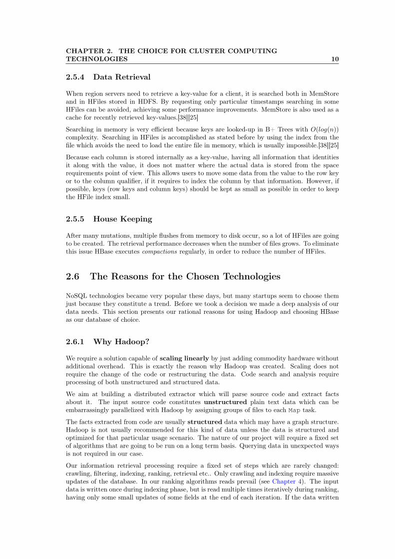
When region servers need to retrieve a key-value for a client, it is searched both in MemStoreand in HFiles stored in HDFS. By requesting only particular timestamps searching in someHFiles can be avoided, achieving some performance improvements. MemStore is also used as acache for recently retrieved key-values.[38][25]
Searching in memory is very efficient because keys are looked-up in B+ Trees with O(log(n))complexity. Searching in HFiles is accomplished as stated before by using the index from thefile which avoids the need to load the entire file in memory, which is usually impossible.[38][25]
Because each column is stored internally as a key-value, having all information that identitiesit along with the value, it does not matter where the actual data is stored from the spacerequirements point of view. This allows users to move some data from the value to the row keyor to the column qualifier, if it requires to index the column by that information. However, ifpossible, keys (row keys and column keys) should be kept as small as possible in order to keepthe HFile index small.
2.5.5 House Keeping
After many mutations, multiple flushes from memory to disk occur, so a lot of HFiles are goingto be created. The retrieval performance decreases when the number of files grows. To eliminatethis issue HBase executes compactions regularly, in order to reduce the number of HFiles.
2.6 The Reasons for the Chosen Technologies
NoSQL technologies became very popular these days, but many startups seem to choose themjust because they constitute a trend. Before we took a decision we made a deep analysis of ourdata needs. This section presents our rational reasons for using Hadoop and choosing HBaseas our database of choice.
2.6.1 Why Hadoop?
We require a solution capable of scaling linearly by just adding commodity hardware withoutadditional overhead. This is exactly the reason why Hadoop was created. Scaling does notrequire the change of the code or restructuring the data. Code search and analysis requireprocessing of both unstructured and structured data.
We aim at building a distributed extractor which will parse source code and extract factsabout it. The input source code constitutes unstructured plain text data which can beembarrassingly parallelized with Hadoop by assigning groups of files to each Map task.
The facts extracted from code are usually structured data which may have a graph structure.Hadoop is not usually recommended for this kind of data unless the data is structured andoptimized for that particular usage scenario. The nature of our project will require a fixed setof algorithms that are going to be run on a long term basis. Querying data in unexpected waysis not required in our case.
Our information retrieval processing require a fixed set of steps which are rarely changed:crawling, filtering, indexing, ranking, retrieval etc.. Only crawling and indexing require massiveupdates of the database. In our ranking algorithms reads prevail (see Chapter 4). The inputdata is written once during indexing phase, but is read multiple times iteratively during ranking,having only some small updates of some fields at the end of each iteration. If the data written

CHAPTER 2. THE CHOICE FOR CLUSTER COMPUTINGTECHNOLOGIES 11
during indexing is structured properly Hadoop performs well when it reads repeatedly duringranking phase.
The last reason for choosing Hadoop is its good support and well written documentation.Being used by major actors from IT, boosts its support and stability making it a reliablesolution.
2.6.2 ACID
RDBMSs generally offer ACID guarantees, which is an abbreviation from atomicity, consistency,isolation and durability. This subsection will explain the concepts and analyze if they arerequired for our system. If not, we can drop some of them in order to gain other advantages.All these guarantees are most of the time linked with the concept of transaction which is a unitof work in a database which may involve more steps.[6]
Atomicity guarantees that a transaction can either be successful or can fail [6]. In case somestep failed in the middle of the transaction, the system must return to the original state whereit was before starting the transaction and declare a failure. HBase guarantees atomic rowmutations [32][38], which meets our requirements for the Generalized CodeRank algorithm. Wedo have updates that expand to more rows at a time and even to more tables during indexingphase, but a failure which will let a data field inconsistent with the other will statistically havean insignificant impact on our system. Besides that such indexing errors are easy to recoverwithout data loss.
Consistency in ACID sense differs from the same concept found in distributed systems whichwill be discussed in the next subsection. Here consistency guarantees that a transaction willbring the system from one valid state to another [6]. This means that if after the transactionsome constraints, triggers or cascades are not valid the transaction must be rolled back and thesystem must return to its original state. So, consistency copes with the logical conditions ofthe system, as opposed to atomicity which copes with failures and errors.
HBase consistency guarantees are linked to its atomic row mutations feature. Retrieval ofa row will return a complete image of that row that existed at some point in history [32].Additionally “time travel” or updates from the past are not possible. HBase does not comewith any other consistency guarantees in ACID sense, but developers are free to implementthis logic in their application either on the client side or on the server side thorough an HBasefeature called coprocessors. This could come with some performance penalties especially whenit is implemented on client side. However for our application ACID-consistency is not required.Logical constraints can be invalidated only through programming errors and there is no reasonto sacrifice performance for constraints checking if those are not very likely to occur.
Isolation ensures that a transaction will not influence other concurrent transactions, i.e., trans-actions are independent of each other [6]. HBase offers atomic row mutations [38] and as aconsequence isolation is guaranteed at the same granularity [32]. It is not very likely that forour applications a higher isolation guarantee is required. We are not planning to run concur-rent algorithms that require atomic operations on multiple rows or tables. We plan to runread queries or distributed, non-concurrent MapReduce algorithms in batch jobs. Most of ourusage patterns will consist of reads. Isolation violations can only occur due to human error orprogramming errors which are expected anyway in a system.
Durability guarantees that when a transaction is reported as successful data mutations willalready be persisted, such that in cause of a system failure (like a power outage) there are nodata losses [6]. HBase aims at offering complete durability through the WAL by ensuring thatany mutation is not reported as successful until writing to the log has not finished. Howeverthere are still issues on this feature and at the time of this writing the only guarantee is that thedata has been flushed to the operating system buffer [42]. If an outage occurs before the buffer

CHAPTER 2. THE CHOICE FOR CLUSTER COMPUTINGTECHNOLOGIES 12
is flushed to disk the data is lost. This is not an HBase issue, but an HDFS one, which hasbeen recently solved [36], but its integration to HBase is pending [21]. It is very likely that thenext HBase version will support full durability. However, small data losses from an unflushedOS buffer are not critical for our applications. Usually our data is obtained from crawling orfrom other data through processing, thus data can be easily recovered.
2.6.3 CAP Theorem and PACELC
Eric Brewer conceived in 2000 the CAP principles, CAP being an abbreviation from consistency,availability and partition-tolerance. In 2002, Nancy Lynch formalized them into a theorem [40]and since then it became a fundamental model for describing distributed databases.
CAP Theorem: It is impossible to have in a distributed system all three qualities of consis-tency, availability and partition-tolerance in the same time.[20][40]
As stated in the previous section, consistency has a different meaning in distributed systemscontext then in ACID. Actually, this semantics is the one which is usually considered whenreferring to the term. Consistency in distributed systems sense subsumes the atomic andconsistent meaning from ACID concepts [40], so it may be defined as atomic consistency.
Consistency in a distributed system (or atomic consistency) guarantees that any observerwill always see the latest version of the data no matter what replica is read.[6][40][20]
Availability ensures that the system will continue to work as a whole even when a node fails,i.e. a response is always received for a request.[40][20]
Partition-tolerance requires a distributed system to continue to operate even if arbitrarilymany messages between two nodes are lost, when a partition in the network appears.
A model for better describing CAP Theorem was proposed by Daniel Abadi, named PACELC[2]. Each letter from this abbreviation is marked with bold and capital letters in the followingscheme:
if Partition:trade between Availability and Consistency
Else:trade between low Latency and Consistency
PACELC model explains the fact that in case of a network partitioning (the P from PACELC)a system needs to make trades between either availability (the A), either consistency (the C).E lse (the E), the system must decide if either providing a low latency (the L) is more importantor a stronger consistency (the C).
As stated atomic consistency covers both the atomicity and consistency terms from ACID.Thus, HBase guarantees the consistency condition in distributed systems terms. Availabilityis weakened in the sense that in case a region server fails it takes some time until the masterreassigns its region and the new assigned region server replays the failed server log (WAL). Bydefault it takes up to three minutes for ZooKeeper to figure out that a region server failed.This can also have implications on latency and data locality in case the data from one of theremaining replicas is not located on the same machine as the new allocated region server. Butthis problem is solved when compactions are performed.
The tradeoff made by HBase at the expense of availability are not a big concern for DistributedSourcerer because the database is not designed to be used by critical realtime applications likecode search. Algorithms are usually using the database, which can be programmed to copewith this kind of situations by waiting for the region to be recovered.

CHAPTER 2. THE CHOICE FOR CLUSTER COMPUTINGTECHNOLOGIES 13
In PACELC semantics, HBase can be characterized as a PC/EC system, because in case of anetwork partition will prefer keeping consistency and weakening availability to some extent andin case of normal operation writes have a larger latency because of the consistency requirementsof the underlying HDFS implementation. Also, latency has to suffer in the case of reassignedregions, but this is just temporarily. However, the consistency is weaker than in RDBMS, suchthat latency is kept within a controllable range.
2.6.4 SQL vs. NoSQL
By applying the CAP Theorem [40] it is know obvious why SQL and RDBMS do not scalefor big data. By ensuring ACID constraints the atomic consistency is guaranteed, which is astrong consistency requirement, which in PACELC semantics translates to a PC/EC distributedsystem. This sacrifices availability and latency for the benefit of consistency. As the systemgrows, the latency also gets larger and parts of the data become unavailable due to failureswhich are normal in a commodity hardware cluster.
As described in the previous section, HBase is also a PC/EC system, but with more relaxedconsistency requirements. Only row mutations are atomic, there are no transactions and noconstraints between columns. By giving up joins, data denormalization and duplication isencouraged, such that only one big table is queried, reducing the overhead. However, this givessome limitations in some scenarios when a relational model is more appropriate.
Another problem with SQL databases are the algorithms they use. Most of them use B+ Treesto store indexes [38], which offer a good performance in O(log(n)) complexity for reads, updatesand inserts. But as the database size grows, more updates are performed and the B+ Trees getimbalanced. Rebalancing is a very expensive operation which can significantly slow down thedatabase. On the other hand, HBase uses a more appropriate design for big data by storing theB+ Trees in the MemStore for recently accessed key-values and by using an index for HFiles,which are stored on disk in HDFS [38]. An overhead occurs during compactions, but those areperformed in two different stages which lowers the impact on performance.
SQL databases are able run on a cluster in a distributed way, but scaling them involves a bigoperational overhead [38]. HBase scales automatically without human intervention. When aregion grows beyond a limit it is automatically split into two regions as described in Section 2.5.
2.7 Summary
We saw in this chapter that HBase by offering atomic row mutations guarantees enough con-sistency for our usage requirements. Reading latency is kept low as the system grows ensuringgood performance for MapReduce. The availability at scale is way more better than what SQLcan offer and the partial outages are controllable and predictable (they are not longer than 3minutes by default). No data losses can occur in case of hardware failures, because mutationsare always persisted to the log first. Since all this HBase advantages fit our needs and alldisadvantages are not a concern for our applications we decided to use HBase to reimplementSourcererDB into what we call SourcererDDB.
Chapter 3
Database Schema Design andQuerying
This chapter presents the motivations behind schema design decisions for the HBase databaseused in Distributed Sourcerer. The former database based on MySQL is also presented bycomparison highlighting differences.
3.1 Database Purpose
As described in Chapter 1.2, Sourcerer uses a database to store information about code entitiesand relations between them, as well as information about projects and files. The extractor parsesJava source files, JARs and class files from the repository in order to extract this informationwhich is described by using the following models [62]:
• Projects: The biggest division in a repository is a project which consists of a set offiles that comprise the same system, are typically developed by the same team and inthe same company or organization. For each project there is a database entry whichstores metadata fields like project name, description, type, version and path within therepository.
• Files: The repository stores Java source files (with .java extension), JAR (Java archive)files (with .jar extension) and Java class files (with .class extension) which are byte codecompiled files contained within the JAR files. Class files not packed into JARs are ignoredby Sourcerer. For each file metadata fields are stored into database like path, file type,file hash and the project ID that contains it.
• Entities: The smallest metamodel divisions extracted from code are represented by en-tities such as methods, variables, classes, interfaces, packages etc.
• Relations: The relationship between entities are modeled by relations such as a callingrelationship between two methods, an inheritance relationship between two classes or acontainment relationship between a class and a method.
Various algorithms can be built on top of the infrastructure to use as input the file structure ofthe projects and the relations between code entities. Chapter 4 describes such an algorithm forcomputing CodeRank, a metric used to rank code entities based on their popularity in a similarway PageRank from Google is used to rank web pages popularity. Code entities relations areused as input to compute CodeRank for each entity from the database.
14

CHAPTER 3. DATABASE SCHEMA DESIGN AND QUERYING 15
The database API can be used to search projects, files, entities and relations matching severalcriteria. For example we can assume that an application needs to retrieve all methods calledfrom a particular class instance, in a particular project. This chapter describes how HBasedatabase was designed in order to facilitate searching based on several matching criteria andhow querying is performed on this schema design.
3.2 Design Principles
All schema design decisions were made such that processing time for database operations isminimized. The most important factor that was considered was reading time because algorithmsthat work with the database perform faster for low latency and high throughput when readingtheir input. Usually only a small number of small size fields are updated in the database. Themost complex writing process takes place at the beginning when the database is populated,but after this stage most operations are reads accompanied by some updates. Some algorithmsrequire reading of large amounts of data in a repeated manner. For instance CodeRank runsiteratively until convergence is reached, so it must read repeatedly all relations from database.In these kind of situations loading large batches of relations into memory with high throughputand low latency are vital. On the other hand writing into the database requires a smalleramount of information to be written in the case of CodeRank. After each iteration the currentCodeRank (a double floating point value) must be written for each entity. The number ofentities is much more smaller than the number of relations.
There is no best design that can perform well in all situations so compromises need to be doneto optimize performance for some particular scenarios. This scenarios were chosen by studyingall MySQL SELECT queries used in Sourcerer as well as studying the data requirements tocompute CodeRank for the entities.
As it was described in Chapter 2, No-SQL schema design principles for databases such asHBase differ substantially from their relational counterparts. Because join operations are notnatively supported and an arbitrary number of columns with arbitrary names can be used fora row, normalization is not required. On the contrary, according to DDI (Denormalization,Duplication, Intelligent keys) principle [19], denormalization should be used instead. Byusing this principle fewer reads are needed to retrieve the data because all the columns requiredcan be stored on the same row, not on different rows from different tables as in relationalnormalized data. Denormalization is often used with duplication if the required data mustbe retrieved by different matching criteria. In this way no secondary indexes must be createdas in SQL databases. In HBase data is sorted by keys, so an intelligent key design must bechosen such that the most common search criteria are optimized. Additionally, as discussed inChapter 2, because data is stored in HFiles as KeyValues, it makes no difference for storagerequirements if data is stored in the key part or in the value part.
3.3 Projects Data
Projects metadata is stored in HBase in a similar way to MySQL. The main difference, detailedin the following sections, lies in the way the row key was designed. The project types definedin Sourcerer are described in Table A.1 [60][62][59].
3.3.1 Former SQL Database
The original MySQL database used in Sourcerer has the columns described in Table 3.1 [60][62][59].Most of the columns can have a null value, thus are optional and important columns like

CHAPTER 3. DATABASE SCHEMA DESIGN AND QUERYING 16
project_id and project_type are indexed for fast retrieval in O(log n).
Table 3.1: Columns for projects MySQL tableColumn Is Indexed Null Descriptionproject_id yes no Numerical unique ID of the project.project_type yes no Type of the project.name yes no Name of the project from the original repository.description no no An optional human readable project description.version no yes Version number for MAVEN projects.groop yes yes Group for MAVEN projects.path no yes Project path within the repository.hash yes yes Project MD5 hash for JAR and MAVEN projects.has_source yes no Whether the project has or does not have source files.
An additional SQL table named project_metrics exists which stores metrics for projectslike the number of lines of code and the number of lines of code with non-whitespace lines. Eachrow contains the project ID, the metric type and the metric value. Thus, a join by project_idis required in order to obtain the metric values for a project.
3.3.2 Functional Requirements
The distributed database should be able to retrieve fast a project by its ID. As it can be seenin the next sections, files, entities and relations are attached to a project by referring to its ID.In case more information about a project is required it can be searched by its ID.
1 SELECT project_id, project_type, path, hash FROM projects2 WHERE project_type = ?
Listing 3.1: SQL Query used to retrieve projects by their type
There are a few methods implemented in Sourcerer that retrieve information about projects bytheir ID by using SQL queries like the one from Listing 3.1. The new database needs to providean efficient way to retrieve project entries by their type.
3.3.3 Schema Design
Each project must be uniquely identified by an ID. An MD5 hash can be used to generate suchan ID. Some of the metadata fields used to describe a project can be hashed to generate theunique MD5. For JAVA_LIBRARY and CRAWLED projects the path from the repository isused as a hash seed since any project has a unique path. But other types of projects do not havethis field so different fields are used to generate an unique ID. For JAR and MAVEN projectsthe hash field is used. For the two SYSTEM projects the ID is a 16 byte array containing theASCII string primitives or unknowns respectively, right padded with null bytes.
Table 3.2: projects HBase TableRow Key <projectType><projectID>Default Column Family name, description, version, groop, path, hasSourceMetrics Column Family linesOfCode, nonWhitespaceLinesOfCode

CHAPTER 3. DATABASE SCHEMA DESIGN AND QUERYING 17
Project metadata is stored into projects HBase table described in Table 3.2. Each projectentry can be assigned to one row creating a tall-narrow table with a lot of rows and just afew columns having the same meaning as the SQL columns in Table 3.1. Part of these fieldscan be stored in the key part to achieve efficient retrieval. All the other columns, which arehomologous to the ones from the SQL schema, can be grouped together as default columnfamily. Because an arbitrary number of columns can be stored on each row there is no need tostore null values, so only those metadata fields that are available can be set as HBase columns.Another column family, named metrics is used to store any metric defined for the project fromthat row. Currently Sourcerer only uses two metrics, but more metrics can be added with nocost in the future.
The main question that arises is how to design the row key for efficient retrieval by both projectID and project type? If the project ID is used as a row key, any project can be efficientlyretrieved with a get operation by using its ID. Using a hash function for all projects IDs, exceptfor the two SYSTEM projects, causes project row entries to be randomly distributed acrossregions, no matter what type they have. So row scans cannot be used to efficiently retrieveprojects by type if project ID is used as row key. Filtering only project rows that have aparticular type is very inefficient because it requires scanning the whole table of projects. Theproject type can be encoded as a single byte and placed in the row key before the 16 byte projectID hash as described in Table 3.2. In this way data locality is achieved and by using row scansall project entries with a particular type can be retrieved. There is no project type that seemsto appear more often than all other types in the dataset so region hotspotting [38] shouldn’tbe a problem. The issue with this approach is that project entries can no longer be retrievedby their ID without knowing the type in advance. If this is not known a get operation can betried for each project type and a particular ID. All this requests can be served in parallel andfor a big dataset requests will be served by different regions exploiting the distributed nature ofHBase. Additionally the number of types to be tried is very small. There are very few projectsof JAVA_LIBRARY type and only two projects of type SYSTEM, so the number of projectsof these types can be neglected. Most of the projects have type CRAWLED and JAR and someof them have type MAVEN. So basically there are only three project types to be tried makingthis approach very efficient.
3.3.4 Querying
As described in Subsection 3.3.3 efficient retrieval of project entries is done when project typeis known. All projects of a particular type can be retrieved by doing row scans. The start rowis set as the 1 byte project type and the stop row is the same byte incremented by 1.
By using a get operation for a row key which includes the project type as the first byte andthe project ID as the rest of the bytes a particular project entry can be retrieved. If projecttype is not known the techniques described previously of trying all types can be applied. Asdescribed, this does not endure serious performance penalties.
Querying by any other other criteria, like path, is not efficient when using this schema design.It is possible to do it by using value filters, but it requires scanning the whole table which cantake a long time.
3.4 Files Data
For files the database only stores metadata as for projects. That is why the schema designfor HBase in this case is also similar to the SQL one. The file types defined in Sourcerer aredescribed in Table A.2[60][62][59].
CHAPTER 3. DATABASE SCHEMA DESIGN AND QUERYING 18
3.4.1 Former SQL Database
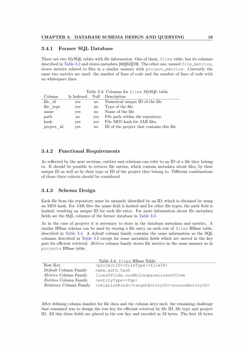
There are two MySQL tables with file information. One of them, files table, has its columnsdescribed in Table 3.3 and stores metadata [60][62][59]. The other one, named file_metrics,stores metrics related to files in a similar manner with project_metrics. Currently thesame two metrics are used: the number of lines of code and the number of lines of code withno whitespace lines.
Table 3.3: Columns for files MySQL tableColumn Is Indexed Null Descriptionfile_id yes no Numerical unique ID of the file.file_type yes no Type of the file.name yes no Name of the file.path no yes File path within the repository.hash yes yes File MD5 hash for JAR files.project_id yes no ID of the project that contains this file.
3.4.2 Functional Requirements
As reflected by the next sections, entities and relations can refer to an ID of a file they belongto. It should be possible to retrieve file entries, which contain metadata about files, by theirunique ID as well as by their type or ID of the project they belong to. Different combinationsof those three criteria should be considered.
3.4.3 Schema Design
Each file from the repository must be uniquely identified by an ID, which is obtained by usingan MD5 hash. For JAR files the name field is hashed and for other file types, the path field ishashed, resulting an unique ID for each file entry. For more information about file metadatafields see the SQL columns of the former database in Table 3.3.
As in the case of projects it is necessary to store in the database metadata and metrics. Asimilar HBase schema can be used by storing a file entry on each row of files HBase table,described in Table 3.4. A default column family contains the same information as the SQLcolumns described in Table 3.3 except for some metadata fields which are moved in the keypart for efficient retrieval. Metrics column family stores file metrics in the same manner as inprojects HBase table.
Table 3.4: files HBase TableRow Key <projectID><fileType><fileID>Default Column Family name, path, hashMetrics Column Family linesOfCode, nonWhitespaceLinesOfCodeEntities Column Family <entityType><fqn>Relations Column Family <relationKind><targetEntityID><sourceEntityID>
After defining column families for file data and the column keys used, the remaining challengethat remained was to design the row key for efficient retrieval by file ID, file type and projectID. All this three fields are placed in the row key and encoded as 33 bytes. The first 16 bytes

CHAPTER 3. DATABASE SCHEMA DESIGN AND QUERYING 19
represent the project ID, the next byte encodes the file type and the last 16 bytes represent thefile ID, as illustrated in Table 3.4. For efficient retrieval of a file entry both the file ID and theID of the project it belongs to need to be known in advance. It is not very important to knowthe file type since all the three types can be tried without sacrificing performance so much.A similar approach was described in Subsection 3.3.3 for trying all project types to retrieve aproject entry. In the case of files, there are even less types to try – only three.
3.4.4 Querying
As discussed in the previous section efficient retrieval of a file entry is achieved when queryingHBase by both file ID and project ID. As discussed, knowing also the file type would not bringsubstantial performance improvements. Knowing the project ID is not a problem for the currentdesign of the database, because as it can be seen in the next sections, when file ID is stored foran entity or relation also the project ID is kept. However, in case project ID is not known, itis possible to retrieve a file entry by using a filter. A custom row filter has been implementedwhich passes all rows that contain into their row key suffix (the last 16 bytes) the file ID. Usingthis retrieval approach is not optimal since it requires scanning of the whole table, but at leastit makes the scenario possible.
Retrieving all files from a project is possible by doing a row scan of all rows that begin with the16 bytes of the project ID. If an additional byte representing the file type is added only files ofa particular type are retrieved from that project.
If it is required to retrieve all files from the repository of a particular type the whole table mustbe scanned and a custom row filter can be used which passes only rows that have the 17th byteset to the correspondent value of the file type.
Querying by other matching fields can be achieved in a non-efficient way by using column valuefilters and scanning the whole table, which can take some time for big datasets.
3.5 Entities Data
Code entities have a lot of information fields that describe them. In order to achieve efficientretrieval by matching several fields duplication design principle [19], described in Section 3.2,will be applied. Thus, entities data will be stored redundantly into multiple HBase tables. Theentity types available in Sourcerer are described in Table A.3 [60][62][59].
3.5.1 Former SQL Database
As in the case of projects and files two MySQL tables are used to store entities information.General information used to describe them is placed in entities table [60] [60][62][59]. Metricinformation is stored in entity_metrics in the same way as for projects and files. Table 3.5describes the columns used in entities SQL table.
3.5.2 Functional Requirements
Schema design for relations HBase tables should provide efficient retrieval by the following datafields:
• FQN (Fully-Qualified Name)

CHAPTER 3. DATABASE SCHEMA DESIGN AND QUERYING 20
Table 3.5: Columns for entities MySQL tableColumn Is Indexed Null Descriptionentity_id yes no Numerical unique ID of the entity.entity_type yes no Type of the entity.fqn yes yes FQN (Fully-Qualified Name) of the entity.modifiers no yes Java modifiers for entity types that are allowed to have them.multi no yes Multipurpose column for additional information.project_id yes no ID of the project that contains the entity.file_id yes yes ID of the file that contains the entity.offset no yes Byte offset of the entity in the source file.length no yes Byte length of the entity in the source file.
• entity type
• project ID
• file ID
This requirements are found in Sourcerer API to the SQL database, where a lot of SQL queriesselect rows by these criteria. For example, Listing 3.2 shows three queries extracted fromSourcerer’s code. All of them filter results by entity type, marking this field as being veryimportant. One of the queries searches entity entries that have a particular FQN prefix, sopartial FQNs should be a searching criteria, not only exact FQNs. The other two queriessearch by project ID and file ID respectively.
1 -- Retrieval by FQN prefix and filtering by entity type:2 SELECT entity_id, entity_type, fqn, project_id FROM entities3 WHERE fqn LIKE ’${PREFIX}%’4 AND entity_type NOT IN (’PARAMETER’, ’LOCAL_VARIABLE’)56 -- Retrival by project ID and filtering by entity type:7 SELECT entity_id, entity_type, fqn, project_id FROM entities8 WHERE project_id = ?9 AND entity_type IN (’ARRAY’, ’WILD_CARD’, ’TYPE_VARIABLE’,
10 ’PARAMETRIZED_TYPE’, ’DUPLICATE’)1112 -- Retrieval by file ID and filtering by entity type:13 SELECT entity_id, entity_type, fqn, project_id FROM entities14 WHERE file_id = ?15 AND entity_type IN (’CLASS’, ’INTERFACE’, ’ANNOTATION’, ’ENUM’)
Listing 3.2: SQL Queries used to retrieve entities data
The former SQL database uses secondary indexes for all these four fields, confirming theirimportance (see Table 3.5).
3.5.3 Schema Design
Entities data is stored redundantly in three HBase tables by applying duplication design prin-ciple [19], thus ensuring efficient retrieval by several criteria.
Each entity is uniquely identified by an MD5 hash ID, calculated by using the following fieldsdescribed in Table 3.5: entity type, FQN, modifiers, multi, project ID, file ID, offset and length.entities_hash HBase table, described in Table 3.6, stores entity data by entity ID. It does

CHAPTER 3. DATABASE SCHEMA DESIGN AND QUERYING 21
this by storing the unique ID as a row key and the other fields as columns in default columnfamily. Entity IDs are used in relations data, so this table can be useful when it is required toretrieve more information about an entity.
Table 3.6: entities_hash HBase TableRow Key <entityID>Default Column Family entityType, fqn, modifiers, multi, projectID, fileID,
fileType, offset, lengthMetrics Column Family linesOfCode, nonWhitespaceLinesOfCodeRelations Column Family sourceEntityType, codeRank, targetEntitiesCount,
targetEntities, relationIDs
To achieve efficient retrieval by the four fields mentioned in the previous section, i.e. FQN,entity type, file ID and project ID, they need to be stored in the key part of two of the tableswhich store entities data, whether this key part is the row key or the column qualifier. Theother remaining fields, which are not stored in the key part, are serialized in the value part.For scenarios when searching by project ID or file ID is required, entities data is stored intofiles HBase table, previously described in Table 3.4 and Subsection 3.4.3. When searchingentities by FQN or FQN prefix a special table is used, named entities table (see Table 3.7).
Table 3.7: entities HBase TableRow Key <fqn>0x00<projectID><fileID>Default Column Family <entityType>
By using the row key design from files table entities can be efficiently searched by projectID, file type and file ID. Entities column family is used to separate entities data from filesmetadata, which is stored in the default and metrics column families as described in Table 3.4.Entity type and FQN fields are placed in this order in the column qualifiers of entities columnfamily.
The one byte entity type and the 16 bytes MD5 hashes for file ID and project ID require exactmatching when performing a search. But for FQN it must be possible to search all entities thathave a particular FQN prefix. The most efficient way to do this is by putting this field at thebeginning of row keys of entities table and performing a scan by the required FQN prefix.After the FQN field the row key includes a null byte which is useful for exact FQN matches.For example let’s assume we need to search an entity which has the exact FQN java.lang.If we perform a scan only by this string other entities with different FQNs but the same prefixwill be returned, such java.lang.Object, java.lang.String etc. But by adding theadditional null byte to the scanning start row string, i.e. "java.lang\0", the exact FQN willbe matched. The next fields found in the row key are the MD5 hashes of project ID and fileID (see Table 3.7), which can help narrowing results by these two other criteria. In all threequeries from Listing 3.3 it is required to narrow the results by including or excluding entitieswith a particular type. By placing the entity type byte in column qualifiers makes this filteringpossible when searching by FQN or FQN prefix. All this columns associated with entity typesare placed into the default column family.

CHAPTER 3. DATABASE SCHEMA DESIGN AND QUERYING 22
3.5.4 Querying
As mentioned in the previous section retrieving en entity entry by its ID is performed inentities_hash table. If entities need to be searched by several criteria the other two tablescan be used, i.e. files table and entities table.
When FQN or an FQN prefix is known, entities table should be used. The following scenarioscover the use cases for this table:
• FQN or an FQN prefix is known
• both the exact FQN and project ID are known
• exact FQN, project ID and file ID are known
Since these three fields presented above are placed in the row key, the scenarios are implementedby doing row scans or using get operations. In the first case the FQN is used as the start rowand in the second the null byte and the project ID are added. In the third case a get operationcan be performed, because by adding the file ID the whole row key is known. Column qualifiershold entity types, so by requesting only some columns to be returned the results are narrowedby the corresponding entity type.
When FQN or an FQN prefix is not known, operations in entities column family of files tableshould be performed. Usually, the use cases of this table are covered when the project ID orfile ID is known. Similar scenarios where presented in Subsection 3.4.4 when searching for files.Here the same matching requirements are desired but for entities instead of files, so entitiescolumn family is used. Narrowing results to some specific entity type can be implemented witha column qualifier prefix filter which passes only those columns that have the required value asthe first byte.
3.6 Relations Data
Storing relations data into HBase requires the same design principle of duplication in order toachieve efficient retrieval for the desired scenarios. Data is stored redundantly in multiple HBasetables, each one being used for a particular scenario. The relation types defined in Sourcererare described in Table A.4 [60][62][59]. Besides its type, a relation also has a class which definesthe location of the target entity as described in Table A.5 [60][62][59].
3.6.1 Former SQL Database
There is only one MySQL table which stores relations data, which is named relations.Table 3.8 describes its columns [60][60][62][59].
3.6.2 Functional Requirements
Retrieval of relation entries should be optimized for the following fields, explained in Table 3.8:
• source entity ID
• target entity ID
• relation type and relation class
• project ID

CHAPTER 3. DATABASE SCHEMA DESIGN AND QUERYING 23
Table 3.8: Columns for relations MySQL tableColumn Is Indexed Null Descriptionrelation_id yes no Numerical unique ID of the relation.relation_type yes no Type of the relation.relation_class no no Class of the relation.lhs_eid yes no ID for the source entity of the relation.rhs_eid yes no ID for the target entity of the relation.project_id yes no ID of the project that contains the relation.file_id yes yes ID of the file that contains the relation.offset no yes Byte offset of the relation in the source file.length no yes Byte length of the relation in the source file.
• file ID
All this requirements can be found in SQL queries from Sourcerer source code, except for sourceentity ID. Two of those SQL queries are available in Listing 3.3. Optimizations for source entityID field were considered for practical reasons and because its column in relations MySQLtable is indexed.
1 -- Retrieve relations by target entity ID and type:2 SELECT project_id FROM relations3 WHERE rhs_eid = ? AND relation_type IN ?45 -- Retrieve relations by project and type:6 SELECT * FROM relations7 WHERE project_id = ? AND relation_type IN ?
Listing 3.3: SQL Queries used to retrieve relations data
3.6.3 Schema Design
Duplication design principle [19] has been applied in order to achieve efficient retrieval by severalcriteria. Thus, relations data has been stored redundantly in multiple HBase tables. Dependingon the application some tables may not be implemented. For example, there is a table namedrelations_hash, described in Table 3.9, which stores relations data by their ID, similar toentities_hash. Currently, there is no feature or algorithm that uses it, so in future it maybe dropped if it’s not required.
Table 3.9: relations_hash HBase TableRow Key <relationID>Default Column Family relationKind, sourceEntityID, sourceEntityType,
targetEntityID, targetEntityType, projectID,fileID, fileType, offset, length
The fields by which the retrieval should be optimized are stored in the key part of the tablesrelations_direct (see Table 3.10), relations_inverse (see Table 3.11) and files(see Table 3.4). The other remaining fields, i.e. offset and length are serialized in the valuepart of those tables.

CHAPTER 3. DATABASE SCHEMA DESIGN AND QUERYING 24
Table 3.10: relations_direct HBase TableRow Key <sourceEntityID><relationKind><targetEntityID>Default Column Family <projectID><fileID>
Table 3.11: relations_inverse HBase TableRow Key <targetEntityID><relationKind><sourceEntityID>Default Column Family <projectID><fileID>
Relation type and relation class are combined together in a single byte in HBase tables resultinga field named relation kind. The three most significant bits are used for relation class and thenext 5 bits for relation type. Relation IDs are calculated by using an MD5 hash on the followingfields: relation kind, source entity ID, target entity ID, project ID, file ID, offset and length.
Efficient retrieval by source entity ID is achieved by querying relations_direct HBasetable, described in Table 3.10, which contains in its row key the following fields in this order:source entity ID (16 bytes), relation kind (1 byte) and target entity ID (16 bytes). Retrievalof all relations with a particular source entity ID and optionally with a particular relationkind is possible through row scanning. The same principles are applied for relations_-inverse table, described in Table 3.11, optimized for retrieval by target entity ID which hasthe following fields in its row key in this order: target entity ID, relation kind, source entity ID.Here scanning can be performed by target entity ID or by both target entity ID and relationkind. Both relations_direct and relations_inverse tables have the same columnkeys design. They have a default column family and column qualifiers contain the project IDand the file ID in this order. Selecting only specific columns or by using column qualifier filtersrelations results can be narrowed to only those that are part of a particular project or sourcefile.
Relations data is also stored in relations column family of files HBase table, described inTable 3.4, similar to entities data in entities column family or to files data in default columnfamily. By using the row key design of this table efficient retrieval by project ID and file IDcan be performed. The other important relation fields are stored in column qualifiers in thefollowing order: relation kind, target entity ID and source entity ID. Narrowing results bymatching this fields is achieved by selecting particular columns or by using column qualifierfilters.
The Generalized CodeRank algorithm described in Chapter 4 gets relations information fromentities_hash table (see Table 3.6), from relations column family. The row key representsthe source entity ID. Target entity IDs of the relations that have this source entity ID, as wellas their relation kinds are serialized in the targetEntities column. The current code rankof the source entity ID defined on the row key is stored in codeRank column.
3.6.4 Querying
A relation entry can be retrieved by its ID by using relations_hash table, which stores theID on the row key.
If efficient retrieval by source entity ID and relation kind or just by source entity ID is desired,relations_direct table should be used. If instead of source entity ID, target entity IDneeds to be matched relations_inverse should be used. Both these two tables have thesame column qualifier design. Requesting specific columns will only retrieve those relations thatare included in the files and projects identified by the columns. If only a particular project is

CHAPTER 3. DATABASE SCHEMA DESIGN AND QUERYING 25
required and all files from the project need to be included a column qualifier prefix filter canbe used which only matches the first 16 bytes of the project ID MD5 hash. A custom filterhas been implemented which can match the last 16 bytes of the qualifier if filtering by file IDis required.
Relations can be efficiently retrieved by project ID, file type and file ID from relations columnfamily of files table. If only those or part of those fields need to be matched the same approachas the one to retrieve files or entities from this table must be applied. Further narrowing of theresults can be performed by selecting specific columns or by using column qualifier filters. Forinstance, the first byte can be matched to select a specific relation kind. The bytes from the2nd to the 17th can be matched to narrow results to a particular target entity ID and finallythe last 16 bytes can be matched for a specific source entity ID (see Table 3.4).
The CodeRank algorithm described in Chapter 4 queries relations data into entities_hashtable, column family relations. The current CodeRank of an entity is also stored here. Efficientretrieval by source entity ID is provided here.
3.7 Dangling Entities Cache
Generalized CodeRank algorithm described in Chapter 4 needs a fast way to retrieve all danglingentities without scanning the whole entities_hash table and checking each entity if it isdangling. Obtaining dangling entities and their CodeRanks can be done by querying danglingentities cache. The cache needs to be rewritten each time a dangling entity’s rank is updated.
Dangling entities cache is implemented by redundantly storing all dangling entities at the endof entities_hash table. This is accomplished through row key design. Each cache entry isa row that has as row keys 16 bytes with the maximum value (FF hex value) followed by adangling entity ID. Because keys are byte ordered the 16 bytes prefix ensures that there is noother entity placed after the cache rows. Performing a row scan having the start row the 16maximum value bytes makes possible the retrieval of all dangling entities.
3.8 Summary
As it can be observed from this chapter, a schema design needs to be engineered for someparticular querying requirements or some data access patterns. A one-size-fits-all design whichworks for every problem is not possible. SQL is more flexible from this point of view, butunfortunately is does not scale to our needs as shown in Chapter 2. This chapter presented ademonstrative schema design which tries to match as close as possible the original Sourcererdata access patterns. All lot of changes can occur to this schema in future development ifneeded.

Chapter 4
Generalized CodeRank
This chapter presents the design of a code analysis algorithm, named Generalized CodeR-ank, which ranks code entities by their popularity within the repository. Inspired by GooglePageRank [63], instead of considering the links between web pages, it uses relations betweencode entities to compute ranks.
4.1 Reputation, PageRank and CodeRank
This section introduces the concept of PageRank, illustrates how it can be applied to codeby introducing the concept of CodeRank and describes how the general concept of PageRankmodels the reputation of nodes within a graph.
4.1.1 PageRank
The PageRank algorithm was first published in the article “The anatomy of a large-scalehypertextual Web search engine” by the Google Inc. founders Brin and Page [10]. Since then,it sparkled a lot of research around it and a lot of variants, improvements and alternativeuses appeared besides its original use for the web. PageRank uses the graph structure of theweb created by the links between web pages to rank those pages’ popularity. The algorithmis inspired by academic citation literature [10] where an article is considered important if alot of other articles cite it. Taking the idea beyond, PageRank ranks higher pages that havemore inbound links and more importantly pages that are linked by other important pages.The algorithm’s philosophy is that when a page links to another page it trusts its content andguarantees for its quality. The same thing happens in the academia, when a paper cites anotherone it takes its content as granted. It is a way to measure a page’ s reputation within the webcontext. If a popular and thus important page, such as one from CNN 1 or Yahoo! 2, links toa web page, it might be ranked higher then another page which has a lot of inbound links fromnon-popular pages.
4.1.2 The Random Web Surfer Behavior
PageRank models the random surfer behavior [10] which starts from a random web page andkeeps following random links without using browser’s back button. After a while he gets bored
1http://www.cnn.com/2http://www.yahoo.com/
26

CHAPTER 4. GENERALIZED CODERANK 27
and jumps to a random page from the web. If he reaches a dangling page, also known as a sinkpage, which has no outbound links, he goes to a random page. The set of all PageRanks canbe viewed like a vector of probability distribution. So the PageRank for a page has a valuebetween 0 and 1 and represents the probability that a user reaches that page by following therandom surfer behavior. Because all PageRanks make up a probability distribution their sumshould be 1.
Web surfing can be modeled with a Markov chain where each page can be viewed as a stateand the links between them are the probabilities of passing to other states. In the case of arandom surfer there is an equal probability to move from one page to another linked page. Morecomplex PageRank models can assign different probabilities in order to better model the realuser behavior which can choose pages by different criteria, such as their topic or the languageare written in or the location of the link on the page.
4.1.3 CodeRank
The general concept of PageRank can be generalized such that the algorithm can be appliedin other fields than the web. To do this, the Web link structure can be viewed as a graphwhere web pages are nodes and links are edges. Thus, for any directed graph PageRank canbe applied. This has been already used in several other fields. One example is a proposal toreplace ISI IF (Institute for Scientific Information, Impact Factor) ranking of science and socialscience journals, which only counts the number of citations for two years, with a PageRank-likeprestige rank.[8] Another usage example is for ecosystem modeling in order to determine whichspecies are important for the health of the environment.[12]
Following this idea, state of the art research in code search and code analysis proposed ap-plications of PageRank to measure the importance of methods, classes, packages and othercode entities [64][51][55]. The name CodeRank for this approach was proposed in an olderimplementation of Sourcerer [51].
The concepts of code entities and relations are explained in Chapter 3. Calculating CodeR-ank follows the principles of PageRank algorithm, but considers entities instead of nodes andrelations between them instead of graph edges. The result is a hierarchy of the most popularentities from the source code used as input. For instance the classes java.lang.Object orjava.lang.String should be very popular for Java source code.
This master thesis proposes a PageRank-like approach to rank all code entities from a reposi-tory following all relations between them, not just for some code entities like methods, classesor packages. From this point, we will refer to the algorithm that follows this approach as Gen-eralized CodeRank. As far as we know calculating PageRank on code entities by taking intoaccount all entities and all relations from a repository has not been done until now.
There are a lot of useful applications for CodeRank:
• Improving results ranking in source code search engines.
• Creating a top of the most important projects from a repository.
• Listing the most important packages, classes and methods from a project to help devel-opers get started with a new project. If they must read the code in order to understandhow it works, they might start with the important packages and read the code of the mostimportant methods of the most important classes.
• In the context of a Web-scale source code repository a top of the most important librariesfor a specific purpose can be computed. This might be useful for project managers thatneed to chose the best library or technology that accomplishes a desired task in theirproject.

CHAPTER 4. GENERALIZED CODERANK 28
As proved by state of the art, CodeRank was successfully used to improve source code searchengines results ranking providing better results to the user.[51][55]
4.1.4 The Random Code Surfer Behavior
The original PageRank algorithm was used in the Web context and models the web surfer be-havior of following links from page to page. Generalized CodeRank could be imagined modelinga programmer’s behavior of surfing source code.
For better understanding we can assume the following scenario. A new developer is hired in acompany to work in a software system implemented in Java which already has a big code baseof multiple tightly coupled projects. Additionally other third-party libraries are used, such asJUnit and Apache Commons. Before the new employee stars coding, it needs to understandhow the already written code works and how it is organized. So he will start from a mainmethod to surf the code to facilitate understanding. While doing this, he will read code entitieslike methods, fields, local variables, classes, packages and follow the relations between them.For example while he reads a method he may follow the call relation to another method and soon. While doing this he may jump to a random point in the source code, i.e. a random entity,from time to time or when he reaches a dangling entity (sink entity), which has no outboundrelations.
By following this model we can interpret CodeRank as the probability that a programmer willencounter an entity while surfing source code. Entities encountered more often are more popularand thus the chance that someone might search them in a source code search engine is bigger.
4.2 Mathematical Model
This section will describe the mathematics behind PageRank concept as it can be applied onany directed graph, no matter if the nodes are web pages, code entities or any other conceptand no matter if the edges are links or code entity relations. However, throughout this sectionwe will use the term CodeRank instead of PageRank, for consistency with the topic describedby this chapter. The concept CodeRank of an entity can be used interchangeably with rank ofan entity.
4.2.1 CodeRank Basic Formula
The CodeRank of an entity is a probability, so it has a value between 0 and 1. When an entityhas outbound relations to other entities it transfers its rank to each of them as illustrated inFigure 4.1. According to the most simple form of CodeRank algorithm an entity rank sums upthe rank amount propagated from all inbound relations as illustrated by the following formula[63]:
R(u) =∑v∈Bu
R(v)
Nv(4.1)
R(u) is the CodeRank of an entity u, Bu is the set of entities that have outbound relations toentity u and Nv is the number of outbound relations of entity v. It can be noticed from theformula that by dividing the rank of an entity by the number of outbound relations, an equalamount of its rank is transfered to each target entity of the outbound relations as it happensin Figure 4.1.

CHAPTER 4. GENERALIZED CODERANK 29
Figure 4.1: CodeRank Example
According to the code surfer model, a programmer might get bored of following relations throughentities and suddenly can jump to a random entity, action known in the literature as telepor-tation [55]. A damping factor d, which represents the probability to follow relations withoutteleporting, is introduced to the previous formula to model this behavior:
R(u) = d∑v∈Bu
R(v)
Nv+ (1− d)
1
n(4.2)
In this formula the value n represents the total number of the entities.
4.2.2 CodeRank Matrix Representation
The set of all CodeRanks for each entity can be grouped together in a vector r. If M is atransition matrix that models code surfer’s behavior of moving from one entity to another, thefollowing formula holds:
r = M · r (4.3)
PageRanks vector r is the dominant eigenvector of the transition matrix M . Computing r fromthe equation is not possible because of the size of matrix M , but the ranks vector r can beapproximated with the formula r = M j ·r0, where r0 is an initial CodeRanks vector. The valuesof the initial ranks are not important because for a large enough j an approximative value of ris obtained. r0 is typically set to an uniform distribution, where each rank is 1/n, n being thesize of the vector. An ideal r would be obtained if j tends to infinity:
r = limj→∞
M j · r0 (4.4)
Transition matrix can be decomposed like this:
M = dP + (1− d)Q = d(A+D) + (1− d)Q (4.5)
d is the damping factor, A is the adjacency matrix which models relations graph, D modelstransitions from dangling entities and Q models teleportation, i.e. random transition to anyentity. Elements ai,j of matrix A are 0 if there is no relation between entity j and entity i. Each

CHAPTER 4. GENERALIZED CODERANK 30
element ai,j represents the probability that the random surfer will go from entity j to entity i.Each column of A sums to 1, making A a stochastic matrix.
From a dangling entity there are no outbound relations, so in order to model random codesurfer behavior, we state that there is equal probability to have an outbound relation to anyother entity. This behavior is modeled by transition matrix D. If an entity j is dangling (sink),then all elements of column j from matrix D are 1/n, because there is equal probability to havea transition to any other entity. Otherwise (j is not dangling), all elements of the column are0. The first equation below describes a way to decompose D, where e is a vector having all itselements 1 and sT is the transposed vector of sink entities, i.e. element j of s is 1 if entity j isdangling and 0 otherwise (4.9).[58]
D = e · sT /n ⇐⇒ D · r = e · (sT · r)/n (4.6)
Computing D · r for CodeRank equation (4.3) is basically reduced to calculating the innerproduct sT · r, as it can be seen in the equations above. Calculating this inner product,referred from now on as dangling entities inner product (DEIP), is equivalent with summingthe CodeRanks of all dangling entities.
By replacing D from (4.6) in (4.5) and M from (4.5) in (4.3) the basic CodeRank formula (4.2)can be rewritten:
R(0)
R(1)
...R(n− 1)
= d
a0,0 a0,1 · · · a0,n−1
a1,0 a1,1 · · · a1,n−1...
.... . .
...an−1,0 an−1,1 · · · an−1,n−1
R(0)
R(1)
...R(n− 1)
+
+d
1
1
...1
[s0 s1 · · · sn−1]
R(0)
R(1)
...R(n− 1)
+ (1− d)
1n1n
...1n
(4.7)
ai,j =
{0 if there is no relation from entity j to entity i1Nj
if there is a relation from entity j to entity i(4.8)
sj =
{0 if j is not a dangling entity1 if j is a dangling entity (4.9)
4.3 Computing Generalized CodeRank with MapReduce
As shown in the previous section, computing CodeRanks vector is performed by repeatedlymultiplying the transition matrix with the current CodeRanks vector. This section will showhow to accomplish this by using Hadoop MapReduce.
4.3.1 Storing Data in HBase
In Chapter 3, Subsection 3.5.3 described how entities_hash HBase table stores data re-quired by Generalized CodeRank algorithm in relations column family. The row key is an entity
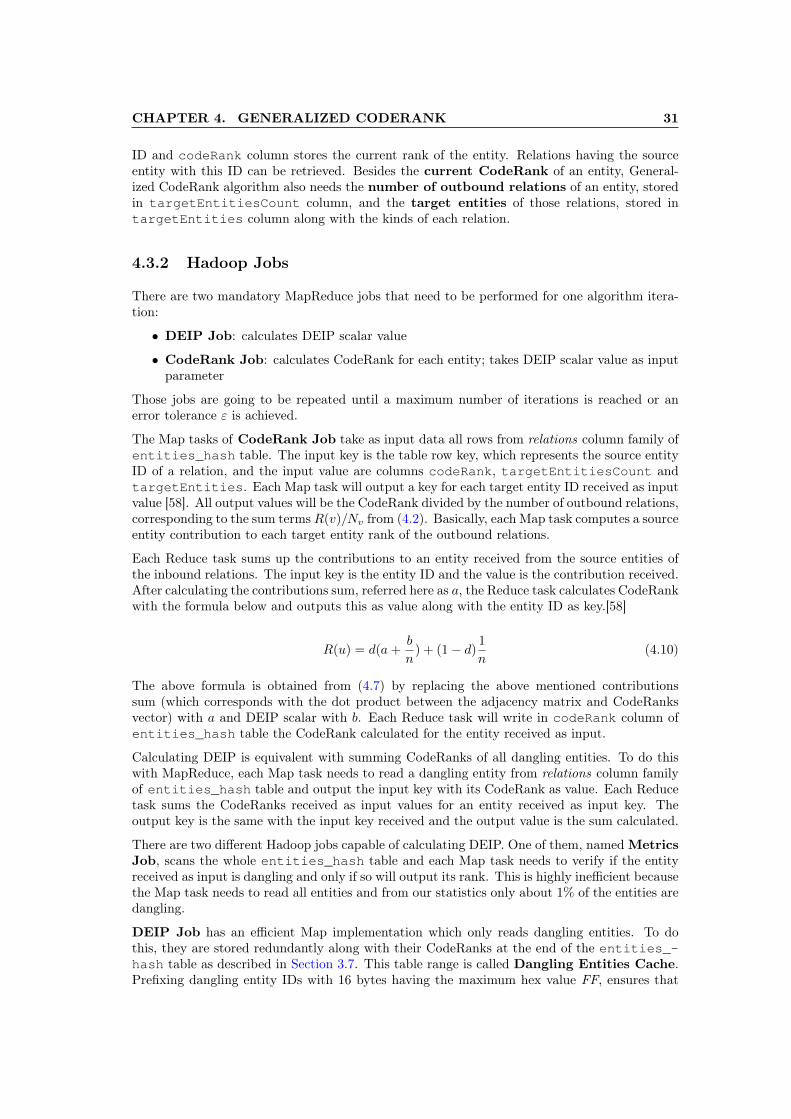
CHAPTER 4. GENERALIZED CODERANK 31
ID and codeRank column stores the current rank of the entity. Relations having the sourceentity with this ID can be retrieved. Besides the current CodeRank of an entity, General-ized CodeRank algorithm also needs the number of outbound relations of an entity, storedin targetEntitiesCount column, and the target entities of those relations, stored intargetEntities column along with the kinds of each relation.
4.3.2 Hadoop Jobs
There are two mandatory MapReduce jobs that need to be performed for one algorithm itera-tion:
• DEIP Job: calculates DEIP scalar value
• CodeRank Job: calculates CodeRank for each entity; takes DEIP scalar value as inputparameter
Those jobs are going to be repeated until a maximum number of iterations is reached or anerror tolerance ε is achieved.
The Map tasks of CodeRank Job take as input data all rows from relations column family ofentities_hash table. The input key is the table row key, which represents the source entityID of a relation, and the input value are columns codeRank, targetEntitiesCount andtargetEntities. Each Map task will output a key for each target entity ID received as inputvalue [58]. All output values will be the CodeRank divided by the number of outbound relations,corresponding to the sum termsR(v)/Nv from (4.2). Basically, each Map task computes a sourceentity contribution to each target entity rank of the outbound relations.
Each Reduce task sums up the contributions to an entity received from the source entities ofthe inbound relations. The input key is the entity ID and the value is the contribution received.After calculating the contributions sum, referred here as a, the Reduce task calculates CodeRankwith the formula below and outputs this as value along with the entity ID as key.[58]
R(u) = d(a+b
n) + (1− d)
1
n(4.10)
The above formula is obtained from (4.7) by replacing the above mentioned contributionssum (which corresponds with the dot product between the adjacency matrix and CodeRanksvector) with a and DEIP scalar with b. Each Reduce task will write in codeRank column ofentities_hash table the CodeRank calculated for the entity received as input.
Calculating DEIP is equivalent with summing CodeRanks of all dangling entities. To do thiswith MapReduce, each Map task needs to read a dangling entity from relations column familyof entities_hash table and output the input key with its CodeRank as value. Each Reducetask sums the CodeRanks received as input values for an entity received as input key. Theoutput key is the same with the input key received and the output value is the sum calculated.
There are two different Hadoop jobs capable of calculating DEIP. One of them, named MetricsJob, scans the whole entities_hash table and each Map task needs to verify if the entityreceived as input is dangling and only if so will output its rank. This is highly inefficient becausethe Map task needs to read all entities and from our statistics only about 1% of the entities aredangling.
DEIP Job has an efficient Map implementation which only reads dangling entities. To dothis, they are stored redundantly along with their CodeRanks at the end of the entities_-hash table as described in Section 3.7. This table range is called Dangling Entities Cache.Prefixing dangling entity IDs with 16 bytes having the maximum hex value FF, ensures that

CHAPTER 4. GENERALIZED CODERANK 32
they are placed at the end of the table. By scanning all rows that start with 16 FF -valuedbytes all dangling entities are retrieved.
Metrics Job can be used to calculate useful metrics:
• Euclidean distance between current CodeRank vector and the one from the previousiteration
• sum of all CodeRanks (should be approximatively 1 if computation was correct)
• DEIP
Generalized CodeRank algorithm continues to run until a maximum number of iterations isreached. An optional stopping condition can be set such that the algorithm stops when a toler-ance is reached, i.e., Euclidean distance metric falls below a threshold ε. When this conditionis set DEIP Job is replaced by Metrics Job which calculates both DEIP scalar and Euclideandistance metric. If desired, also sum can be calculated. Metrics Job is inefficient for DEIP cal-culation, but if calculating metrics is desired, this compromise must be done, because Euclideandistance and sum require all CodeRanks of all entities.
4.4 Experiments
This section presents our experiments with the Generalized CodeRank algorithm by describingour data input, the infrastructural setup and the results accompanied by statistical remarks.
4.4.1 Setup
A sample repository of about 333 MiB was used to populate the database. We did not testedwith a bigger repository because currently the extractor is not yet ported to run on the clus-ter. Populating our HBase database involves a lot of overhead because at the moment we areimporting data from the old MySQL database, which takes a lot of time. After running the ex-tractor the HBase database contained 111 projects, 29, 236 files, 611, 262 entities and 1, 936, 757relations.
Hadoop and HBase were deployed on an 9 node cluster reserved from Tembusu Cluster ofNational University of Singapore, School of Computing. Each is a Dell PC with 2 x Quad-Core Xeon E5620 2.4GHz CPU, 24 GiB RAM. It runs CensOS GNU/Linux operating systeminstalled on a 500 GiB hard-disk. Two additional hard-disks are used to store HDFS data, eachwith 1 TiB, connected in a RAID matrix.
On one node we run the HBase master, Hadoop JobTracker and HDFS NameNode. On eachof the others we placed HBase RegionServers, Hadoop TaskTrackers and HDFS DataNodes.Three of these former nodes hosted a ZooKeeper cluster.
4.4.2 Convergence
In a first experiment 29 iterations of Generalized CodeRank algorithm have been run and foreach one the Euclidean distance between the current CodeRank vector and the one from theprevious iteration has been calculated. Figure 4.2 shows how this Euclidean distance varieswith each iteration. A desired tolerance of 10−5 is reached after 15 iterations, which is enoughfor good CodeRank results.

CHAPTER 4. GENERALIZED CODERANK 33
Figure 4.2: Variation of Euclidean distance with the growth of iteration illustrating the conver-gence of Generalized CodeRank algorithm
When metrics like Euclidean distance are calculated, Metrics Job instead of DEIP Job is exe-cuted. In order to test with DEIP Job also, another experiment was run with 15 iteration. Theresults shown in the next subsectios are obtained from this second experiment.
4.4.3 Probability Distribution
The mathematical model of CodeRank states that CodeRanks vector is a probability distribu-tion. This distribution is plotted in Figure 4.3 for the first 40 largest CodeRank values. Theranks are ordered in decreasing order and indexed from 0 to 38. x axis has index values and yaxis has rank values.
Figure 4.3: Probability distribution represented by CodeRanks vector
It is known from previous studies that PageRank follows a power law distribution with the powervalue of approximatively 1 [71]. Figure 4.4 plots the CodeRanks distribution obtained from thesecond experiment and a power law distribution f(x) modeled by the following equation:
f(x) =max(r)
x+ 1(4.11)

CHAPTER 4. GENERALIZED CODERANK 34
Figure 4.4: log-log plot for CodeRanks distribution and a power law distribution
r is the CodeRanks vector and max(r) is the biggest CodeRank, i.e., the one that has indexx = 0 in Figure 4.3. Both axes of Figure 4.4 are on logarithmic scale, so PageRank points havecoordinate (logx, logR(x)) and power law’s points have (logx, logf(x)).
log f(x) = logmax r
x+ 1⇐⇒ log f(x) = logmax r − log (x+ 1) ⇐⇒
⇐⇒ g(log (x+ 1)) = k − log (x+ 1) ⇐⇒ g(x) = k − x(4.12)
In the above equation log f(x) = g(log (x+ 1)) and k = logmax r is a constant. Equationg(x) = k − x which describes the power law from Figure 4.4 is linear, so its graphic is aline. The CodeRank points from the figure are very close to the power law line, proving thatCodeRanks follow a power law distribution like PageRanks from the web.
4.4.4 Entities CodeRank Top
Table 4.1 describes the 10 entities with the largest CodeRank expressed as percents. An ex-tended version of this table which shows 100 entities instead of 10 can be found in Appendix BTheir importance in the repository is very big because those 10 entities from a total of 611, 262sum 21.42% from the total amount of CodeRank as illustrated in the right side of Figure 4.5.
Table 4.1: Top 10 Entities CodeRank# Entity Type FQN CodeRank1 package java.lang 4.72%2 primitive void 4.24%3 class java.lang.Object 4.06%4 primitive int 2.29%5 class java.lang.String 2.20%6 primitive boolean 1.12%7 package java.io 1.03%8 interface java.io.Serializable 1.00%9 interface java.lang.CharSequence 0.39%10 parametrized type java.lang.Comparable<java.lang.String> 0.37%

CHAPTER 4. GENERALIZED CODERANK 35
Figure 4.5: Left: Top 10 Entities CodeRank chart; Right: Distribution of Top 10 EntitiesCodeRanks within the whole set of entities
It can be observed that the 10 most popular entities are all either from the Java StandardLibrary or are primitives ubiquitous in any Java application. The reason for this is thatany Java program need them in order to work. java.lang, which takes the first place, isthe default package, so it’s imported by default. Any program should have at least a mainmethod, which has type void, primitive that occupies the second place. The base of all classesis java.lang.Object – third place. A Java program must have at least one class which bydefault inherits Object.
We can conclude that the correctness of the results is justified by both the relevance of CodeR-anks Top and also by having the same statistical model (i.e. CodeRank and PageRank followthe same power law distribution).
4.4.5 Performance Results
Table 4.2 contains the time required by Generalized CodeRank to run the experiments, as wellas the time for each job involved in the process.
Table 4.2: Experiments and jobs running timeExperiment / Job TimeExperiment 1 (with metrics), 29 iterations 4485 s (74 min 45 s)Experiment 2 (without metrics), 15 iterations 1882 s (31 min 22 s)Experiment 3 (with metrics), 15 iterations 2255 s (37 min 35 s)DEIP Job (for Experiment 2) 41 sMetrics Job (for Experiment 1 and 3) 69 s (1 min 9 s)CodeRank Job 84 s (1 min 24 s)
As explained in this chapter DEIP, can be calculated either with a DEIP Job or a Metrics Job.The results from the table show that by using dangling entities cache, DEIP Job achieves aperformance boost of 68.29%. The computation of Generalized CodeRank as a whole benefitsfrom a performance boost of 19.82%.

Chapter 5
Implementation
The original Sourcerer code search infrastructure has been developed in Java at UniversityCalifornia of Irvine. This master thesis describes the work around a fork of Sourcerer, namedDistributed Sourcerer, which aims at scaling up Sourcerer to Internet-scale.
The original database implementation, which relied on MySQL, has been rewritten from scratchin order to work with HBase. The implementation details and the new API to the database isdescribed in Section 5.1. A higher level interface to the new database, as a set of command-lineinterface (CLI) tools, is described in Section 5.3.
The Generalized CodeRank algorithm, described in Chapter 4, has been implemented overHadoop MapReduce as described in Section 5.2. A CLI user interface which facilitates CodeR-ank calculation is described in Section 5.6.
5.1 Database Implementation
The new distributed database implementation is called SourcererDDB and is located indistributed-database Eclipse project, path “infrastructure/tools/java/distributed-database” fromDistributed Sourcerer repository [11]. Its implementation can be divided into three parts de-scribed in the next subsections:
• Subsection 5.1.1: classes used to model data, HBase tables and model types
• Subsection 5.1.2: classes that provide the programming interface to retrieve data fromHBase tables
• Subsection 5.1.3: classes that provide the programming interface to insert data to HBasetables
• Subsection 5.1.4: Hadoop MapReduce jobs which duplicates data into additional tablesfor efficient retrieval
5.1.1 Data Modeling
The data modeling part of the implementation is compounded from three Java packages de-scribed as follows:
1. edu.nus.soc.sourcerer.ddb.tables
• Eclipse project: distributed-database
36

CHAPTER 5. IMPLEMENTATION 37
• Path: infrastructure/tools/java/distributed-database/src/edu/nus/soc/sourcerer/ddb/tables/
• Description: classes from this package contain information about HBase tables andprovide access to them.
2. edu.uci.ics.sourcerer.model
• Eclipse project: model
• Path: infrastructure/tools/java/model/src/edu/uci/ics/sourcerer/model/
• Description: this package contains classes that abstract the model types describedin Appendix A for projects, files, entities and relations.
3. edu.nus.soc.sourcerer.model.ddb
• Eclipse project: distributed-database
• Path: infrastructure/tools/java/distributed-database/src/edu/nus/soc/sourcerer/model/ddb/
• Description: classes used to abstract data exchanged with HBase in an object-oriented way.
Each HBase table has an associated class from package edu.nus.soc.sourcerer.ddb.tables,named <name>HBTable. <name> identifies the table, so the camel case of the table namewas chosen. So, for example, relations_inverse HBase table is associated with classRelationsInverseHBTable.
All classes associated with tables follow singleton design pattern and extend HBTable abstractclass. A unique instance of a class is obtained with getInstance()method. The only abstractmethod that needs to be overridden is getName(), which returns the associated table’s name.The base class HBTable provides the implementation of getHTable() method which returnsan HTable instance for the associated table, which is used to access the table as described inHBase documentation [38]. When the instance is created for the first time setupHTable()methods is called, where special configuration code for an HTable instance can be added.
Besides the table name, classes associated with tables also contain static final fields whichstore column family names and column qualifier names. An HTableDescriptor (see HBasedocumentation [38]) can be obtained by calling the static method getTableDescriptor().The obtained instance can be used to create new tables, modify tables schema, delete tablesetc.. These administrative operations are implemented in class DatabaseInitializer frompackage edu.nus.soc.sourcerer.ddb.tools. Updating tables schema is not currentlyimplemented and a NotImplementedException is thrown.
Package edu.uci.ics.sourcerer.model, which contains enums that abstract model types,was included in the original Sourcerer implementation. Project types, file types, entity types, re-lation types and relation classes are abstracted in classes Project, File, Entity, Relationand RelationClass, respectively. I modified those classes in order to encode a byte valuefor each type, which can be returned by using getValue() method.
Classes from package edu.nus.soc.sourcerer.model.ddb are used to model data ex-changed with HBase. All of them implement Model interface and have their name ended inModel. Some of them implement the interface indirectly by extending class ModelWithID.Method computeId from this class returns an MD5 hash of the class fields passed as param-eters. The data from those fields is obtained through Java reflection and the returned valuecan be used to set an id field for a model. For most models that extend ModelWithID this isdone in the constructor.

CHAPTER 5. IMPLEMENTATION 38
5.1.2 Database Retrieval Queries API
Package edu.nus.soc.sourcerer.ddb.queries from Eclipse project distributed-databaseprovides specialized classes to retrieve and add data about projects, files, entities and relationsdata. Listing 5.1 presents an example of retrieving relations by several criteria.
1 try {2 /* Instatiate the object used to retrieve relations3 from HBase.*/4 RelationsRetriever rr = new RelationsRetriever();56 /* Results are going to be printed as they are retrieved7 from HBase.*/8 ModelAppender<Model> appender = new PrintModelAppender<Model>();9
10 /* Retrieve relations call.*/11 rr.retrieveRelations(appender, sourceID, kind, targetID,12 projectID, fileID, fileType);13 } catch (HBaseConnectionException e) {14 LOG.fatal("Could not connect to HBase database: "15 + e.getMessage());16 } catch (HBaseException e) {17 LOG.fatal("An HBase error occured: "18 + e.getMessage());19 }
Listing 5.1: Retrieving relations example
In order to retrieve logical entries from HBase, referred from now as models, the following APIsteps must be followed. Each step is exemplified in Listing 5.1. The models are implementedin package edu.nus.soc.sourcerer.model.ddb.
1. A retrieval class is used to search HBase tables.
• In the example from Listing 5.1, RelationsRetriever class is used.
2. A retrieval method of that class is called. The first parameter is always a ModelAppenderobject. Subsequent parameters represent several searching criteria. If one of these pa-rameters is null, searching will not be performed by that criteria. Depending on whatsearching criteria parameters are not null, the method will figure out in which HBasetable to look up for the entries in order to optimize the query.
• In the example, method retrieveRelations from line 11 is called. After the appender,the following searching criteria are passed respectively: source entity ID, relation kind(byte representing relation type and relation class), target entity ID, project ID, file IDand file type. Depending on which of these criteria parameters are null, HBase will look inrelations_direct, relations_inverse or files table.
3. Inside the retrieval method, HBase client API is used which retrieves table rows as results.In some tables each row is mapped to exactly one model, but in others a row is mappedto multiple models. A result-to-model(s) method is used to convert a table row resultto a model or a set of models.
• In the example, HBase client API will retrieve table rows as results from relations_-direct, relations_inverse or files table, depending on the criteria parameterswhich are not null. In relations_hash table each row is mapped to exactly one re-lation entry, but in relations_direct or relations_inverse tables, a row may con-tain more relation entries. relationsInverseResultToRelationsGroupedModels
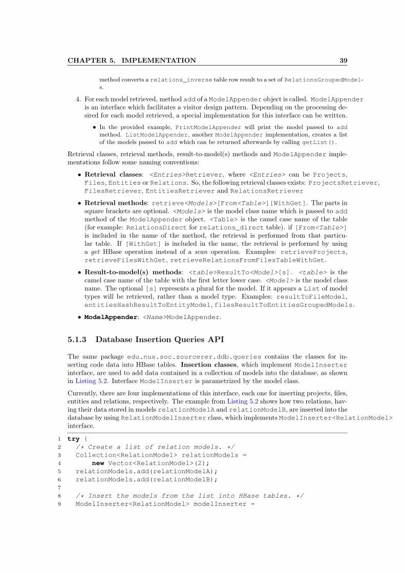
CHAPTER 5. IMPLEMENTATION 39
method converts a relations_inverse table row result to a set of RelationsGroupedModel-s.
4. For each model retrieved, method add of a ModelAppender object is called. ModelAppenderis an interface which facilitates a visitor design pattern. Depending on the processing de-sired for each model retrieved, a special implementation for this interface can be written.
• In the provided example, PrintModelAppender will print the model passed to addmethod. ListModelAppender, another ModelAppender implementation, creates a listof the models passed to add which can be returned afterwards by calling getList().
Retrieval classes, retrieval methods, result-to-model(s) methods and ModelAppender imple-mentations follow some naming conventions:
• Retrieval classes: <Entries>Retriever, where <Entries> can be Projects,Files, Entities or Relations. So, the following retrieval classes exists: ProjectsRetriever,FilesRetriever, EntitiesRetriever and RelationsRetriever
• Retrieval methods: retrieve<Models>[From<Table>][WithGet]. The parts insquare brackets are optional. <Models> is the model class name which is passed to addmethod of the ModelAppender object. <Table> is the camel case name of the table(for example: RelationsDirect for relations_direct table). if [From<Table>]is included in the name of the method, the retrieval is performed from that particu-lar table. If [WithGet] is included in the name, the retrieval is performed by usinga get HBase operation instead of a scan operation. Examples: retrieveProjects,retrieveFilesWithGet, retrieveRelationsFromFilesTableWithGet.
• Result-to-model(s) methods: <table>ResultTo<Model>[s]. <table> is thecamel case name of the table with the first letter lower case. <Model> is the model classname. The optional [s] represents a plural for the model. If it appears a List of modeltypes will be retrieved, rather than a model type. Examples: resultToFileModel,entitiesHashResultToEntityModel, filesResultToEntitiesGroupedModels.
• ModelAppender: <Name>ModelAppender.
5.1.3 Database Insertion Queries API
The same package edu.nus.soc.sourcerer.ddb.queries contains the classes for in-serting code data into HBase tables. Insertion classes, which implement ModelInserterinterface, are used to add data contained in a collection of models into the database, as shownin Listing 5.2. Interface ModelInserter is parametrized by the model class.
Currently, there are four implementations of this interface, each one for inserting projects, files,entities and relations, respectively. The example from Listing 5.2 shows how two relations, hav-ing their data stored in models relationModelA and relationModelB, are inserted into thedatabase by using RelationModelInserter class, which implements ModelInserter<RelationModel>interface.
1 try {2 /* Create a list of relation models. */3 Collection<RelationModel> relationModels =4 new Vector<RelationModel>(2);5 relationModels.add(relationModelA);6 relationModels.add(relationModelB);78 /* Insert the models from the list into HBase tables. */9 ModelInserter<RelationModel> modelInserter =

CHAPTER 5. IMPLEMENTATION 40
10 new RelationModelInserter(2);11 modelInserter.insertModels(relationModels);12 } catch (HBaseException e) {13 LOG.fatal("An HBase error occured: "14 + e.getMessage());15 }
Listing 5.2: Inserting relations example
All ModelInserter implementations should have their name following the format <ModelClass>Inserter.ProjectModelInserter adds data to projects table, FileModelInserter to filestable, EntityModelInserter inserts data to entities_hash table and RelationModelInserterto relations_hash table.
Currently class MySQLImporter uses all these insertion classes mentioned to import code datafrom the old MySQL database (SourcererDB) to the new database (SourcererDDB), based onHBase. The next section shows how the new imported data is indexed into more tables forefficient retrieval.
5.1.4 Indexing Data from Database
The insertion classes described in the previous subsection only populate one table for each ofthe metamodels projects, files, entities and relations. This tables are basically hash tables forefficient retrieval by MD5 hash ID. In order to have an optimized retrieval by several othersearching criteria, other tables need to be populated for redundancy, as explained in Chapter 3.To achieve this some Hadoop MapReduce jobs need to be run. By running those jobs duplicationand denormalization principles are satisfied for the data [38]. For projects and files, two HBasetables are enough. But for entities and relations storing data redundantly is required.
All Hadoop MapReduce classes are currently organized in distributed-database Eclipse project.Classes which implement MapReduce Job-s are placed in edu.nus.soc.sourcerer.ddb.mapreduce.jobspackage, Map classes in edu.nus.soc.sourcerer.ddb.mapreduce.map, and Reduceclasses in edu.nus.soc.sourcerer.ddb.mapreduce.reduce.
In order to index entities a MapReduce job needs to be run. Its class name, as well as theircorresponding Map and Reduce class implementations are as follows:
• EntitiesIndexerJob: indexes entities by duplicating their data from entities_-hash table to entities table and entities column family of files table.
– Map task class: EntitiesMapper
– Reduce task class: EntitiesReducer
In order to index relations two MapReduce jobs need to be run. Their class names, as well astheir corresponding Map and Reduce class implementations are as follows:
• RelationsIndexerJob: indexes relations by duplicating their data from relations_-hash table to relations_direct table, relations_inverse table and relationscolumn family of files table.
– Map task class: RelationsMapper
– Reduce task class: RelationsReducer
• CRRelationsIndexerJob: indexes relations for efficient retrieval during CodeRankcalculation. Data from relations_hash table is redundantly stored in relations columnfamily of entities_hash table, as explained in Chapter 4.

CHAPTER 5. IMPLEMENTATION 41
– Map task class: RelationsSourceMapper
– Reduce task class: RelationsSourceReducer
5.2 CodeRank Implementation
Chapter 4 explained in details what MapReduce jobs are required to calculate CodeRank andhow these jobs need to be combined and repeated in order to achieve a final result. As aconsequence, most of Subsection 5.2.1 will specify which classes are used for each job and whichmap and reduce task classes are used for them. Subsection 5.2.2 will describe some additionalutility jobs that have been implemented.
Generalized CodeRank source code is located in distributed-database Eclipse project. The samepackage structure for MapReduce jobs, Map tasks and Reduce tasks was used as specified inSubsection 5.1.4.
5.2.1 CodeRank and Metrics Calculation Jobs
If the database has just been populated and indexed, the values from relations column fam-ily of entities_hash table need to be initialized. An initialization job does the followingoperations:
• The initial CodeRank for all entities is set to 1/n, where n is the total number ofentities.
• Dangling Entities Cache is created with its initial values of CodeRank (1/n, as previ-ously stated).
• For entities with no outbound relations, target entities count column must store avalue of 0, such that they can be identified as dangling entities in a MetricsJob.
CodeRank and metrics calculation job class names, as well as their corresponding Map andReduce class implementations are as follows:
• CRInitJob: the initialization job described above.
– Map task class: CRInitMapper
– Reduce task class: not available
• CRJob: the CodeRank Job described in Subsection 4.3.2.
– Map task class: CRMapper
– Combine task class: CRCombiner
– Reduce task class: CRReducer
• DEIPJob: the DEIP Job described in Subsection 4.3.2.
– Map task class: DEIPMapper
– Combine task class: DEIPReducer
– Reduce task class: DEIPReducer
• CRMetricsJob: the Metrics Job described in Subsection 4.3.2.
– Map task class: CRMetricsMapper
– Combine task class: CRMetricsCombiner
CHAPTER 5. IMPLEMENTATION 42
– Reduce task class: CRMetricsReducer
5.2.2 Utility Jobs
Currently there is only one utility job which is used to output in an HDFS text file the entitiestop by their CodeRank. Entities formatted in descendant order are each stored on a line. Thereare four tab separated columns:
• CodeRank (as a subunit value, not percent)
• entity ID (hex representation of the MD5 hash)
• entity types
• FQN (Fully-Qualified Name)
The job class name, as well as their corresponding Map and Reduce class implementations areas follows:
• CRTop
– Map task class: CRTopMapper
– Reduce task class: not available
5.3 Database Querying Tools
Database querying tools have their source code in Eclipse project distributed-database, mainclass edu.nus.soc.sourcerer.ddb.tools.Main.
When running the tools at the command line their name and their arguments are prefixed bydouble-minus --. The following list presents the tools. Parameter --help for any tool willprint usage information, including arguments explanation. All tools that work with the HBasedatabase support --hbase-table-prefix, which appends the specified prefix to all tablenames that are going to be accessed. Argument --properties-file can be used to pass aJava properties file where predefined arguments are stored as key-value pairs, separated by theequal = sign.
• --retrieve-projects: search projects from the database
– --pt: project type as upper case string
– --pid: project ID as a hex of the MD5 hash
• --retrieve-files: search files from the database
– --pid: project ID as a hex of the MD5 hash
– --ft: file type as upper case string
– --fid: file ID as a hex of the MD5 hash
• --retrieve-entities: search entities from the database
– --eid: entity ID as a hex of the MD5 hash
– --et: entity type as upper case string
– --fqn: fully-qualified name
– --fqn-prefix: fully-qualified name prefix

CHAPTER 5. IMPLEMENTATION 43
– --pid: project ID as a hex of the MD5 hash
– --fid: file ID as a hex of the MD5 hash
– --ft: file type as upper case string
• --retrieve-relations: search relations from the database
– --rid: relation ID as a hex of the MD5 hash
– --seid: source entity ID as a hex of the MD5 hash
– --teid: target entity ID as a hex of the MD5 hash
– --rk: relation kind as upper case string compound from relation type and relationclass separated by a double colon
– --fqn: fully-qualified name
– --fqn-prefix: fully-qualified name prefix
– --pid: project ID as a hex of the MD5 hash
– --fid: file ID as a hex of the MD5 hash
– --ft: file type as upper case string
• --retrieve-relations-by-source: retrieve relations by source entity ID from re-lations column family, entities_hash table
– --eid: entity ID as a hex of the MD5 hash
• --retrieve-code-rank: prints the CodeRank of an entity by its ID
– --eid: entity ID as a hex of the MD5 hash
5.4 Database Utility Tools
Utility tools share the same main class as querying tools. The following list presents the tools:
• --initialize-db: tool used to initialize HBase database by creating the tables
– --empty-existing: if a table already exists, it is empty (by deleting it andcreating it again)
– --update-existing: if a table already exists, its configuration and column fam-ilies definition is updated if necessary. This feature is not currently implemented
• --import-mysql: imports data from an old SourcererDB database, based on MySQL
– --database-url
– --database-user
– --database-password
5.5 Database Indexing Tools
Database indexing tools are used to duplicate data in multiple tables for efficient retrieval asdiscussed in Section 5.1.4 and have their main classes located in distributed-database project,in package edu.nus.soc.sourcerer.ddb.mapreduce. Tools that use Hadoop have adifferent library for parsing command-line arguments. Other database tools rely on Sourcerer

CHAPTER 5. IMPLEMENTATION 44
library, but database indexing and CodeRank tools rely on Apache Commons library. For eachHadoop tool there is a different main class and arguments have both a short one letter formprefixed by one hyphen - and a long form prefixed by two hyphens --. There is a set of commonarguments for all tools described in Table 5.1.
Table 5.1: Common CLI arguments for Hadoop tools (CodeRank and Database indexing tools)Long arg. Short arg. Description--hbase-table-prefix -p Prefix appended to HBase table names--debug -d Turn on debug
In order to index entities, the tool with the main class EntitiesIndexer must be used. Toindex relations, the tool with the main class RelationsIndexer must be used.
5.6 CodeRank Tools
CodeRank tools are basically used for CodeRank calculation and have their main classes locatedin distributed-database project, in package edu.nus.soc.sourcerer.ddb.mapreduce. Be-ing Hadoop applications they also use Apache Commons CLI arguments parsing library, asexplained in the previous section.
The most important tool is the one used to calculate CodeRanks for all entities. Its main classis CodeRankCalculator and the command line arguments are described in Table 5.2.
Arguments --num-iter and --entities-count are mandatory. If the initialization jobneeds to be run as explained in Subsection 5.2.1, then --init argument must be set. If it is de-sired to iterate the algorithm until a tolerance is reached --tolerance argument must be pro-vided with a small floating point value. Setting this requires setting --metric-euclidian-distancealso. By setting any argument which starts with --metric-, Metric Job will be used insteadof DEIP Job, as discussed in Subsection 4.3.2. The performance is affected, but it is the onlyway to do it if metric calculation or iterating until a tolerance is reached is required.
Another tool which has its main class CodeRankUtil is used to exclusively calculate metrics orto output in HDFS a text file with entities top by CodeRank. Its CLI arguments are describedin Table 5.3.

CHAPTER 5. IMPLEMENTATION 45
Table 5.2: Common CLI arguments for CodeRankCalculator toolLong arg. Short arg. Description--num-iter -n The number of CodeRank iterations to
run--init -i Initialize database before CodeRank
calculation. Required if tables has justbeen populated
--entities-count -c The number of entities--teleportation-probab -r Probability of jumping from one entity
to another random one. Defaults to0.15
--metric-euclidian-distance -e Calculate euclidian distance betweencurrent CodeRank vector and the pre-vious one. Use --tolerance / -t argu-ment to set a distance when computa-tion should stop
--tolerance -t Euclidian distance between currenct it-eration and the previous one whichstops computation if it is reached. Re-quires setting --metric-euclidian-dist /-e argument
--metric-coderanks-sum -s Calculate the sum of CodeRanks for allentities. Should be close to 1 if compu-tation was correct
--metrics-output -o Output directory in HDFS where met-rics should be saved (one file foreach iteration). This argument is ig-nored if calculation of no metric isrequested. One of the arguments --metric-euclidian-dist / -e or --metric-coderanks-sum / -s should be set. Out-put file(s) will contain by default anadditional metric which is “deip” (dan-gling entities inner product)
Table 5.3: Common CLI arguments for CodeRankUtil toolLong arg. Short arg. Description--coderank-top -T Generate a file with the top of all entities by
CodeRank--metric-euclidian-dist -e Calculate euclidian distance between current
CodeRank vector and the previous one--metric-coderanks-sum -s Calculate the sum of CodeRanks for all enti-
ties. Should be close to 1 if computation wascorrect
--metric-deip -D Calculate DEIP (Dangling Entities InnerProduct)

Chapter 6
Conclusions
This chapter exposes a summary of the contributions of this work, presents an outlook of futureresearch to the “Semantic-based Code Search” project and takes a look to the past by comparingthis work with state of the art contributions.
6.1 Summary
I have chosen a cluster computing technology stack, based on Hadoop and HBase, as a basis foran Internet-scale code search and code analysis platform. By performing a rigorous analysis Iproved that an SQL database would not scale for our needs because of the big latencies involved.We showed that the tradeoff made by moving to HBase, such as giving up some consistencyguarantees affects our applications in a negligible way. The system can now scale linearly byjust adding new commodity hardware machines and benefits from using the popular HadoopMapReduce platform, which is highly used in the industry and has a big community around it,both of volunteers and of companies with commercial interest.
I have engineered an HBase database schema design for the storage layer of the system. Itallows basic code queries to be performed and stores the data needed to calculate General-ized CodeRank. I have showed that there is no schema that meets any application need andexemplified why the chosen schema wouldn’t be appropriate for other data access patterns.
I implemented [11] a PageRank variant for ranking code entities, which as far we know it isunique by considering all entities during calculation and not only subsets of particular types.I proved the validity of the results by coming with both statistical proofs and intuitive facts.Those results show that CodeRank gives relevant results even when all entity types are con-sidered during computation. The algorithm was implemented over Hadoop MapReduce andterminates in reasonable time – about 30 minutes for a Java repository of about 300 MiB. Theranked entities improve code search as state of the art shows [51][55].
6.2 Future Work
The next step for building our code search engine is the parallelize the extractor such that itcan run on a cluster. Our idea is to use Hadoop for this purpose by running on each Map anextractor instance. The files need to be accessible to each Map. Putting files in HDFS is not agood idea, because this file system performs good for sequential access to big files, but sourceand jar files are small. To address this issue we could write source files in HBase, because are
46
CHAPTER 6. CONCLUSIONS 47
small enough to fit as values. Additionally random access to particular files is possible withgood performance. Jar files can embed a lot of files, hence they can grow larger and storingthem in HBase can create problems [31]. This files can be stored in HDFS as SequenceFiles, byconcatenating multiple jars in a big HDFS file. Thus, sequential access is achieved for optimumMapReduce performance. The only drawback is having a bigger overhead for random access toa particular jar file.
The second task that we want to accomplish in the future is scaling up the search server. Asdiscussed in Chapter 2, Sourcerer uses Solr as a search server. Its distributed version, namedDistributed Solr [30], is currently limited in comparison with single machine Solr. We areconsidering to use ElasticSearch [18] instead of Solr, which also uses Lucene [26] and performsbetter than Solr for realtime access to a large-scale index [67].
Our third plan is linked to a contribution we want to make to code search field. We arecurrently investigating a way to improve the results by using code clone detection techniquesand clustering.
6.3 Related Work
Besides Sourcerer [4] from which our system has been forked there are several other infrastruc-tures for code search or code analysis. Portfolio [55] is a code search system for C programminglanguage which focuses on retrieval and visualization of relevant functions and their usages.Similar to my work it implements PageRank for code, but it only uses functions and their callrelation. Besides this, it also proposes a technique called SAN (Spreading Activation Network)to improve ranking. For the purpose of indexing, it uses Lucene like Sourcerer.
An older version of Sourcerer use to implement CodeRank [51], but currently this component isnot available any more. Another search tool that relies on Sourcerer is CodeGenie [50], whichuses test-cases to search and reuse source code.
Another code search engine which uses test-cases is a prototype of Reiss et al. presented in [66].Besides test-cases and standard keyword based retrieval techniques it also uses contracts andsecurity constraints. The distinctive characteristic of this engine is its ability to apply programtransformations to adapt to user requirements.
Keinvaloo et al. proposed another Internet-scale code search infrastructure called SE-CodeSearch[45], based on semantic web. Instead of relying on a relational model like Sourcerer, this in-frastructure uses an ontology to represent facts about source code and inference to acquire newknowledge about missing code entities.
For the purpose of querying source code based on its entities and relations, different other math-ematical models have been proposed besides relational algebra (used in relational databases)and description logics (used in semantic-web ontologies). It is important to notice that the stor-age solution proposed in this work, although it uses HBase which is not a relational database,it uses a relational model.
Query languages using relational algebra have been implemented, like SemmleCode [70] andJGraLab [17]. Similar to Codd’s relational algebra is Tarski’s Binary Relational Calculus [69].Grok [43], Rscript [46] and JRelCal [65] use this formalism. Other approaches use predicatelogic like CrocoPat [7] and JTransformer [47].

Appendix A
Model Types
Table A.1: Project TypesProject Type DescriptionSYSTEM Project type used for only two core projects. One of them groups prim-
itive types provided by the Java language and the other one unknownentities with unresolved references.
JAVA_LIBRARY Projects associated Java Standard Library JARs, like rt.jar.CRAWLED Projects downloaded by the crawler from online repositories.JAR All unique JARs aggregated from the CRAWLED projects are also
considered a project on their own.MAVEN Used for MAVEN projects.[27]
Table A.2: File TypesFile Types DescriptionSOURCE Files containing Java source code from any project except SYSTEM.CLASS Files containing Java byte code from any project except SYSTEM and
CRAWLED. Class files are extracted from jar files. The extractor ignorescrawled class files which are not packed into a jar.
JAR Jar files from CRAWLED projects.
48

APPENDIX A. MODEL TYPES 49
Table A.3: Entity TypesEntity Type DescriptionUNKNOWN used for an undefined typePACKAGE package declarationCLASS class declarationINTERFACE interface declarationENUM enum declarationANNOTATION annotation declarationINITIALIZER for instance or static initializer declarationFIELD field declarationENUM_CONSTANT enum constant declarationCONSTRUCTOR constructor declarationMETHOD method declarationANNOTATION_ELEMENT annotation type element declarationPARAMETER formal parameter declarationLOCAL_VARIABLE local variable declarationPRIMITIVE only used in primitives SYSTEM projectARRAY array declarationTYPE_VARIABLE type variable declarationWILDCARD wildcard declarationPARAMETRIZED_TYPE parametrized type declarationDUPLICATE an entity created when it is unclear exactly
which type was referenced by a relation

APPENDIX A. MODEL TYPES 50
Table A.4: Relation TypesRelation Types DescriptionUNKNOWN used for an undefined type.INSIDE physical containment. Example: METHOD INSIDE
CLASS.EXTENDS class inheritance. Example: CLASS EXTENDS CLASS.IMPLEMENTS interface implementation or inheritance. Example: CLASS
IMPLEMENTS INTERFACE or INTERFACE IMPLE-MENTS INTERFACE.
HOLDS defines the type of a field. Example: FIELD HOLDS CLASS.RETURNS defines the return type of a method. Example: METHOD
RETURNS CLASS.READS a field being read. Example: METHOD READS FIELD.WRITES a field being written. Example: METHODWRITES FIELD.CALLS method invocation. Example: METHOD CALLS
METHOD.USES type reference. Example: METHOD USES CLASS.INSTANTIATES constructor invocation for object instantiation. Example:
METHOD INSTANTIATES CONSTRUCTOR.THROWS defines a throws clause. Example: METHOD THROWS
CLASS.CASTS defines a cast expression. Example: METHOD CASTS
CLASS.CHECKS defines an instanceof expression: METHOD CHECKS
CLASS.ANNOTATED_BY an entity is annotated. Example: METHOD ANNO-
TATED_BY CLASS.HAS_ELEMENTS_OF defines the item type from an array. Example: ARRAY
HAS_ELEMENTS_OF CLASS.PARAMETRIZED_BY defines the type parameters for an entity. Example:
METHOD PARAMETRIZED_BY TYPE_VARIABLE.HAS_BASE_TYPE defines the base type of a parametrized type. Example:
PARAMETRIZED_TYPE HAS_BASE_TYPE CLASS.HAS_TYPE_ARGUMENT defines the bounding of a type parameter to a specific
type. Example: PARAMETRIZED_TYPE HAS_TYPE_-ARGUMENT CLASS.
HAS_UPPER_BOUND defines the upper bound of a wildcard. Example: WILD-CARD HAS_UPPER_BOUND CLASS.
HAS_LOWER_BOUND defines the lower bound of a wildcard. Example: WILD-CARD HAS_LOWER_BOUND CLASS.
OVERRIDES defines when a method overrides a parent class/interfacemethod. Example: METHOD OVERRIDES METHOD.
MATCHES defines when a DUPLICATE type matches a number oftypes. Example: DUPLICATE MATCHES CLASS.
Table A.5: Relation ClassesRelation Classes DescriptionUNKNOWN It is unknown where the target entity is.JAVA_LIBRARY The target entity is located in the JAVA_LIBRARY project.INTERNAL The target entity is in the same project.EXTERNAL The target entity is in an external project.NOT_APPLICABLE It makes no sense to classify the target entity as internal or external.

Appendix B
Top 100 Entities CodeRank
Table B.1: Top 100 Entities CodeRank (No. 1-33)# Entity Type FQN CodeRank1 package java.lang 4.715620%2 primitive void 4.242388%3 class java.lang.Object 4.059280%4 primitive int 2.293895%5 class java.lang.String 2.199717%6 primitive boolean 1.116965%7 package java.io 1.034111%8 interface java.io.Serializable 1.000685%9 interface java.lang.CharSequence 0.388675%10 parameterized type java.lang.Comparable<java.lang.String> 0.374038%11 package java.util 0.304947%12 primitive long 0.251881%13 interface java.lang.Comparable 0.232919%14 package java.awt 0.222480%15 interface java.lang.Cloneable 0.221790%16 primitive byte 0.200660%17 package javax.swing 0.195239%18 type variable <T+java.lang.Object> 0.163133%19 primitive short 0.155148%20 class java.lang.Exception 0.139547%21 package java.sql 0.138024%22 package sun.awt.X11 0.136395%23 unknown java.lang.Object 0.136028%24 package org.w3c.dom 0.130180%25 primitive float 0.108922%26 type variable <E+java.lang.Object> 0.099308%27 primitive double 0.096172%28 package javax.accessibility 0.094041%29 class java.lang.Throwable 0.089935%30 package org.omg.CORBA 0.089068%31 package com.lowagie.text.pdf 0.088002%32 class java.util.Vector 0.087758%33 class java.util.ListResourceBundle 0.087504%
51

APPENDIX B. TOP 100 ENTITIES CODERANK 52
Table B.2: Top 100 Entities CodeRank (No. 34-67)# Entity Type FQN CodeRank34 primitive char 0.083407%35 interface javax.accessibility.Accessible 0.080270%36 interface org.w3c.dom.Node 0.079507%37 class javax.swing.JComponent 0.075495%38 package org.xml.sax 0.074926%39 package sun.org.mozilla.javascript 0.073773%40 interface java.util.List 0.072944%41 interface java.util.EventListener 0.071246%42 package org.biomage.Interface 0.070408%43 unknown java.lang.String 0.067242%44 class java.lang.Class 0.066851%45 package net.sf.pizzacompiler.compiler 0.065243%46 package java.lang.reflect 0.063781%47 class java.io.InputStream 0.062156%48 type variable <E> 0.060435%49 package java.awt.event 0.059796%50 package ru.novosoft.uml.foundation.core 0.059524%51 array byte[] 0.058651%52 package com.sun.java.swing.plaf.nimbus 0.058159%53 package org.hsqldb 0.057687%54 package org.hsqldb 0.057557%55 class java.awt.Color 0.057352%56 class java.awt.Component 0.056617%57 package javax.swing.text 0.056141%58 class java.io.File 0.055589%59 package com.sun.media.sound 0.054086%60 package java.security 0.052590%61 package com.sun.org.apache.bcel.internal.generic 0.051423%62 package javax.swing.plaf.basic 0.050802%63 package com.ibm.db2.jcc.b 0.050419%64 interface org.w3c.dom.Element 0.049696%65 class java.util.Hashtable 0.049590%66 class java.util.ResourceBundle 0.049359%67 interface java.lang.Runnable 0.048984%

APPENDIX B. TOP 100 ENTITIES CODERANK 53
Table B.3: Top 100 Entities CodeRank (No. 68-100)# Entity Type FQN CodeRank68 interface java.util.Collection 0.048234%69 constructor java.lang.Object.<init>() 0.047192%70 package java.awt.image 0.046850%71 package antlr 0.046490%72 interface java.util.Map 0.045774%73 class java.sql.SQLException 0.045667%74 interface java.sql.Wrapper 0.045381%75 package javax.swing.plaf 0.045180%76 interface java.io.Closeable 0.045055%77 package java.net 0.044337%78 package xjavadoc 0.043616%79 package com.sun.org.apache.xalan.internal.xsltc.compiler 0.043496%80 class javax.swing.JPanel 0.042380%81 package org.w3c.dom.svg 0.042105%82 package ca.gcf.util 0.041985%83 class com.sun.java.swing.plaf.nimbus.AbstractRegionPainter 0.041813%84 class java.lang.RuntimeException 0.041065%85 class java.lang.Integer 0.040916%86 class java.io.OutputStream 0.040798%87 class com.sun.corba.se.impl.logging.ORBUtilSystemException 0.039915%88 class java.io.Writer 0.038651%89 class java.awt.Container 0.038380%90 package com.lowagie.text 0.038072%91 package java.nio 0.037661%92 interface java.util.Iterator 0.037292%93 array java.lang.String[] 0.037119%94 type variable <V+java.lang.Object> 0.036814%95 package com.ibm.db2.jcc.a 0.036752%96 interface java.sql.ResultSet 0.036514%97 interface sun.awt.X11.XKeySymConstants 0.036440%98 class java.util.ArrayList 0.036350%99 class com.sun.corba.se.spi.logging.LogWrapperBase 0.035903%100 package javax.management 0.035815%

Bibliography
[1] Inc. 10gen. MongoDB. http://www.mongodb.org/, August 2012.
[2] Daniel Abadi. Problems with CAP, and Yahoo’s little known NoSQL system. http://dbmsmusings.blogspot.ro/2010/04/problems-with-cap-and-yahoos-little.html, April 2010.
[3] Amitanand S. Aiyer, Mikhail Bautin, Guoqiang Jerry Chen, Pritam Damania, PrakashKhemani, Kannan Muthukkaruppan, Karthik Ranganathan, Nicolas Spiegelberg, LiyinTang, and Madhuwanti Vaidya. Storage Infrastructure Behind Facebook Messages: UsingHBase at Scale. IEEE Data Eng. Bull., 35(2):4–13, 2012.
[4] Sushil Bajracharya, Joel Ossher, and Cristina Lopes. Sourcerer: An internet-scale softwarerepository. In Proceedings of the 2009 ICSE Workshop on Search-Driven Development-Users, Infrastructure, Tools and Evaluation, SUITE ’09, pages 1–4, Washington, DC, USA,2009. IEEE Computer Society.
[5] Sushil Krishna Bajracharya, Joel Ossher, and Cristina Videira Lopes. Leveraging usagesimilarity for effective retrieval of examples in code repositories. In Gruia-Catalin Romanand Kevin J. Sullivan, editors, SIGSOFT FSE, pages 157–166. ACM, 2010.
[6] Daniel Bartholomew. SQL vs. NoSQL. Linux Journal, 2010(195), Jully 2010.
[7] D. Beyer, A. Noack, and C. Lewerentz. Efficient relational calculation for software analysis.31:137– 149, 2005.
[8] Johan Bollen, Marko A. Rodriguez, and Herbert Van de Sompel. Journal status. Sciento-metrics, volume 69, number 3, pp. 669-687, 2006, December 2006.
[9] Dhruba Borthakur, Jonathan Gray, Joydeep Sen Sarma, Kannan Muthukkaruppan, Nico-las Spiegelberg, Hairong Kuang, Karthik Ranganathan, Dmytro Molkov, Aravind Menon,Samuel Rash, Rodrigo Schmidt, and Amitanand Aiyer. Apache hadoop goes realtime atfacebook. In Proceedings of the 2011 ACM SIGMOD International Conference on Man-agement of data, SIGMOD ’11, pages 1071–1080, New York, NY, USA, 2011. ACM.
[10] Sergey Brin and Lawrence Page. The anatomy of a large-scale hypertextual web searchengine. Comput. Netw. ISDN Syst., 30(1-7):107–117, April 1998.
[11] Călin-Andrei Burloiu. Distributed sourcerer code on github. https://github.com/calinburloiu/Sourcerer, September 2012.
[12] Judith Burns. Google trick tracks extinctions. http://news.bbc.co.uk/2/hi/science/nature/8238462.stm, September 2009.
[13] Fay Chang, Jeffrey Dean, Sanjay Ghemawat, Wilson C. Hsieh, Deborah A. Wallach, MikeBurrows, Tushar Chandra, Andrew Fikes, and Robert E. Gruber. Bigtable: A distributedstorage system for structured data. ACM Trans. Comput. Syst., 26(2):4:1–4:26, June 2008.
[14] Codase. Codase. http://www.codase.com/, September 2012.
54

BIBLIOGRAPHY 55
[15] Jeffrey Dean and Sanjay Ghemawat. MapReduce: Simplified Data Processing on LargeClusters. InOSDI ’ 04: Sixth Symposium on Operating System Design and Implementation,San Francisco, CA, 2004.
[16] Giuseppe DeCandia, Deniz Hastorun, Madan Jampani, Gunavardhan Kakulapati, AvinashLakshman, Alex Pilchin, Swaminathan Sivasubramanian, Peter Vosshall, and Werner Vo-gels. Dynamo: amazon’s highly available key-value store. SIGOPS Oper. Syst. Rev.,41(6):205–220, October 2007.
[17] Jürgen Ebert, Daniel Bildhauer, Hannes Schwarz, and Volker Riediger. Using DifferenceInformation to Reuse Software Cases. Softwaretechnik-Trends, 27(2), 2007.
[18] Elasticsearch. Elasticsearch. http://www.elasticsearch.org/, September 2012.
[19] D. Salmen et al. Cloud data structure diagramming techniques and de-sign patterns. https://www.data-tactics-corp.com/index.php/component/jdownloads/finish/22-white-papers/68-cloud-data-structure-diagramming, November 2009.
[20] Dietrich Featherston. Cassandra: Principles and application. http://dfeatherston.com/cassandra-cs591-su10-fthrstn2.pdf.
[21] Apache Software Foundation. Allow proper fsync support for HBase. https://issues.apache.org/jira/browse/HBASE-5954, August 2012.
[22] Apache Software Foundation. Apache cassandra. http://cassandra.apache.org/, September2012.
[23] Apache Software Foundation. Apache CouchDB. http://couchdb.apache.org/, August 2012.
[24] Apache Software Foundation. Apache hadoop. http://hadoop.apache.org/, September 2012.
[25] Apache Software Foundation. Apache HBase. http://hbase.apache.org/, September 2012.
[26] Apache Software Foundation. Apache lucene. http://lucene.apache.org/, September 2012.
[27] Apache Software Foundation. Apache Maven Project. http://maven.apache.org/, August2012.
[28] Apache Software Foundation. Apache software foundation. http://www.apache.org/,September 2012.
[29] Apache Software Foundation. Apache solr. http://lucene.apache.org/solr/, September 2012.
[30] Apache Software Foundation. Distributed solr. http://wiki.apache.org/solr/DistributedSearch, September 2012.
[31] Apache Software Foundation. HBase – FAQ Design. http://wiki.apache.org/hadoop/Hbase/FAQ_Design#A3, September 2012.
[32] Apache Software Foundation. HBase ACID Properties. http://hbase.apache.org/acid-semantics.html, September 2012.
[33] Apache Software Foundation. HBase/PoweredBy - Hadoop Wiki. http://wiki.apache.org/hadoop/Hbase/PoweredBy, September 2012.
[34] Apache Software Foundation. HDFS architecture guide. http://hadoop.apache.org/docs/r1.0.3/hdfs_design.html, August 2012.
[35] Apache Software Foundation. Powered by – hadoop wiki. http://wiki.apache.org/hadoop/PoweredBy, September 2012.
[36] Apache Software Foundation. Support hsync in HDFS. https://issues.apache.org/jira/browse/HDFS-744, August 2012.

BIBLIOGRAPHY 56
[37] Eclipse Foundation. Eclipse. http://eclipse.org/, September 2012.
[38] Lars George. HBase: The definitive guide. O’Reilly, September 2011.
[39] Sanjay Ghemawat, Howard Gobioff, and Shun-Tak Leung. The google file system. SIGOPSOper. Syst. Rev., 37(5):29–43, October 2003.
[40] Seth Gilbert and Nancy Lynch. Brewer’s conjecture and the feasibility of consistent, avail-able, partition-tolerant web services. SIGACT News, 33(2):51–59, June 2002.
[41] Derrick Harris. How Facebook keeps 100 petabytes of Hadoop data online. http://gigaom.com/cloud/how-facebook-keeps-100-petabytes-of-hadoop-data-online/, September 2012.
[42] Lars Hofhansl. HBase, HDFS and durable sync. http://hadoop-hbase.blogspot.ro/2012/05/hbase-hdfs-and-durable-sync.html, May 2012.
[43] Richard C. Holt. Structural manipulations of software architecture using tarski relationalalgebra. In Proceedings of the Working Conference on Reverse Engineering (WCRE’98),WCRE ’98, pages 210–, Washington, DC, USA, 1998. IEEE Computer Society.
[44] Patrick Hunt, Mahadev Konar, Flavio P. Junqueira, and Benjamin Reed. Zookeeper: wait-free coordination for internet-scale systems. In Proceedings of the 2010 USENIX conferenceon USENIX annual technical conference, USENIXATC’10, pages 11–11, Berkeley, CA,USA, 2010. USENIX Association.
[45] Iman Keivanloo, Laleh Roostapour, Philipp Schugerl, and Juergen Rilling. SE-CodeSearch:A scalable Semantic Web-based source code search infrastructure. In Proceedings of the2010 IEEE International Conference on Software Maintenance, ICSM ’10, pages 1–5,Washington, DC, USA, 2010. IEEE Computer Society.
[46] Paul Klint. How understanding and restructuring differ from compiling – a rewritingperspective. In Proceedings of the 11th IEEE International Workshop on Program Com-prehension, IWPC ’03, pages 2–, Washington, DC, USA, 2003. IEEE Computer Society.
[47] Gunter Kniesel and Uwe Bardey. An analysis of the correctness and completeness of aspectweaving. In Proceedings of the 13th Working Conference on Reverse Engineering, WCRE’06, pages 324–333, Washington, DC, USA, 2006. IEEE Computer Society.
[48] Koders. Koders. http://koders.com/, September 2012.
[49] Krugle. Krugle. http://krugle.com/, September 2012.
[50] Otávio Augusto Lazzarini Lemos, Sushil Krishna Bajracharya, and Joel Ossher. Codege-nie: : a tool for test-driven source code search. In Richard P. Gabriel, David F. Bacon,Cristina Videira Lopes, and Guy L. Steele Jr., editors, OOPSLA Companion, pages 917–918. ACM, 2007.
[51] Erik Linstead, Sushil Bajracharya, Trung Ngo, Paul Rigor, Cristina Lopes, and PierreBaldi. Sourcerer: mining and searching internet-scale software repositories. Data Miningand Knowledge Discovery, 18:300–336, 2009.
[52] Amazon Web Services LLC. Amazon s3. http://aws.amazon.com/s3/, August 2012.
[53] Karma Snack LLC. Search engine market share. http://www.karmasnack.com/about/search-engine-market-share/, September 2012.
[54] M. Loukides. What is data science? http://radar.oreilly.com/2010/06/what-is-data-science.html, August 2012.
[55] Collin McMillan, Mark Grechanik, Denys Poshyvanyk, Qing Xie, and Chen Fu. Portfolio:finding relevant functions and their usage. In Proceedings of the 33rd International Con-

BIBLIOGRAPHY 57
ference on Software Engineering, ICSE ’11, pages 111–120, New York, NY, USA, 2011.ACM.
[56] memcached. memcached. http://memcached.org/, August 2012.
[57] neo4j.org. Neo4j graph database. http://neo4j.org/, August 2012.
[58] Michael Nielsen. Using MapReduce to compute PageRank. http://michaelnielsen.org/blog/using-mapreduce-to-compute-pagerank/, January 2009.
[59] University California of Irvine. Sourcerer code on github. https://github.com/sourcerer/Sourcerer, September 2012.
[60] University California of Irvine. SourcererDB web page. http://sourcerer.ics.uci.edu/sourcerer-db.html, September 2012.
[61] Oracle. MySQL. http://www.mysql.com/, September 2012.
[62] Joel Ossher, Sushil Bajracharya, Erik Linstead, Pierre Baldi, and Cristina Lopes. Sourcer-erDB: An aggregated repository of statically analyzed and cross-linked open source javaprojects. In Proceedings of the 2009 6th IEEE International Working Conference on Min-ing Software Repositories, MSR ’09, pages 183–186, Washington, DC, USA, 2009. IEEEComputer Society.
[63] Lawrence Page, Sergey Brin, Motwani Rajeev, andWinograd Terry. The PageRank citationranking: Bringing order to the web. Technical report, Stanford University, 1998.
[64] Diego Puppin and Fabrizio Silvestri. The social network of java classes. In Proceedings ofthe 2006 ACM symposium on Applied computing, SAC ’06, pages 1409–1413, New York,NY, USA, 2006. ACM.
[65] Peter Rademaker. Binary relational querying for structural source code analysis. 2008.
[66] Steven P. Reiss. Semantics-based code search. In Proceedings of the 31st InternationalConference on Software Engineering, ICSE ’09, pages 243–253, Washington, DC, USA,2009. IEEE Computer Society.
[67] Ryan Sonnek. Realtime Search: Solr vs Elasticsearch. http://blog.socialcast.com/realtime-search-solr-vs-elasticsearch/, May 2011.
[68] Michael Stonebraker. SQL databases v. NoSQL databases. Commun. ACM, 53(4):10–11,April 2010.
[69] A. Tarski. On the calculus of relations. Journal of Symbolic Logic, 6(3):73–89, September1941.
[70] Mathieu Verbaere, Elnar Hajiyev, and Oege de Moor. Improve software quality withSemmleCode: an eclipse plugin for semantic code search. In Richard P. Gabriel, David F.Bacon, Cristina Videira Lopes, and Guy L. Steele Jr., editors, OOPSLA Companion, pages880–881. ACM, 2007.
[71] Yana Volkovich, Nelly Litvak, and Debora Donato. Determining factors behind the PageR-ank log-log plot. In Proceedings of the 5th international conference on Algorithms and mod-els for the web-graph, WAW’07, pages 108–123, Berlin, Heidelberg, 2007. Springer-Verlag.
[72] Tom White. Hadoop: The definitive guide (third edition). O’Reilly, Yahoo! Press, January2012.
[73] Wikipedia. Big data. http://en.wikipedia.org/wiki/Big_data, August 2012.


![[slides] Parallel and Distributed Computing on Low Latency Clusters](https://static.fdocuments.us/doc/165x107/5466a74cb4af9ff5748b4830/slides-parallel-and-distributed-computing-on-low-latency-clusters.jpg)
