1

Distributed Algorithms for Optimal Power FlowProblem

Albert Y.S. Lam, Baosen Zhang, and David Tse

Abstract—Optimal power flow (OPF) is an important problemfor power generation and it is in general non-convex. Withthe employment of renewable energy, it will be desirable ifOPF can be solved very efficiently so its solution can be usedin real time. With some special network structure, e.g. trees,the problem has been shown to have a zero duality gap andthe convex dual problem yields the optimal solution. In thispaper, we propose a primal and a dual algorithm to coordinatethe smaller subproblems decomposed from the convexified OPF.We can arrange the subproblems to be solved sequentially andcumulatively in a central node or solved in parallel in distributednodes. We test the algorithms on IEEE radial distribution testfeeders, some random tree-structured networks, and the IEEEtransmission system benchmarks. Simulation results show thatthe computation time can be improved dramatically with ouralgorithms over the centralized approach of solving the problemwithout decomposition, especially in tree-structured problems.The computation time grows linearly with the problem size withthe cumulative approach while the distributed one can have size-independent computation time.

I. INTRODUCTION

AN ELECTRIC power system is the main facility todistribute electricity in modern societies. It is a network

connecting power supplies (e.g., thermoelectric generators andturbine steam engines) to consumers. A power grid is generallycomposed of several subsystems: generation, transmission,substation, distribution, and consumers. The generators gen-erate power which is delivered to the substations at highvoltages through the transmission network. The power voltageis stepped down and then distributed to the consumers viathe distribution networks. In a typical power system, a fewhundreds of generators interconnect to several hundreds ofsubstations. The substations distribute the power to millions ofconsumers with relatively simpler radial networks with tree-like structures.

In the past, research on power systems mainly focusedon the core of the network, i.e., from the generation, viatransmission, to the substations. All of the control, planningand optimization was done by a single entity (e.g. an ISO).With the integration of renewal energy and energy storage,self-healing ability, and demand response, the focus is shiftedtoward the consumer side, i.e. distribution networks, and thisnew paradigm is called the smart grid [1].

The optimal power flow (OPF) is one of the most importantproblems in power engineering and it aims to minimize thegeneration cost subject to demand constraints and the network

The authors are with the Department of Electrical Engineering and Com-puter Sciences, University of California, Berkeley, CA, 94720 USA (e-mail:ayslam, zhangbao, dtse@eecs.berkeley.edu).

physical constraints, e.g. bus voltage limits, bus power limits,thermal line constraint, etc. Due to the quadratic relationsbetween voltage and power, OPF is non-convex. In general,heuristic approaches have been employed to solve the OPFbut they are not guaranteed to yield the optimal solution. Tosimplify the calculation, with assumptions on lossless powerline, constant voltage and small voltage angles, OPF canbe linearized and this approximation is also called DC-OPF,which is not accurate under all circumstances [2]. For thecomplex OPF, [3] suggested solving the problem in its dualform and studied the conditions of the power network withzero duality gap. In [4], it was shown that the duality gapis always zero for network structures such as trees whichmodel distribution networks well. [5], as an independent workof this paper, decomposes the OPF in terms of cycles andbranches and formulates the problem as an second-order coneprogram for tree networks which is equivalent to that given in[6]. In traditional power systems, OPF is mainly for planningpurpose. For example, it is used to determine the system statein the day-ahead market with the given system information.In the smart grid paradigm, due to highly intermittent natureof the renewable, the later the prediction is made, the morereliable it is. If OPF can be solved very efficiently, we maysolve the OPF in real time thus mitigating some of theunpredictability.

We aim at solving OPF efficiently. When the system size(e.g. the number of buses) increases, solving the problemin a centralized manner is not practical (this will be veri-fied in the simulation). One possible way is to tackle theproblem distributedly by coordinating several entities in thesystem, each of which handle part of the problem and theircollaborative effort solves the whole problem. To do this, acommunication protocol is needed to define what informationshould be conveyed among the entities. We can learn fromthe networking protocol development to design a commu-nication protocol for OPF. The earliest form of protocolsfor the Internet was proposed in 70’s. They were designedto handle the increasing volume of traffic sent over theInternet in an ad hoc manner. In 1998, Kelly et al. studiedTransmission Control Protocol (TCP), which is one of thecore protocols in TCP/IP [7]. They showed that TCP can beanalyzed with a fundamental optimization problem for ratecontrol and the algorithms developed from the optimizationfit the ad hoc designed variants of TCP. This lays down aframework to design communication protocols for complexsystems with reasoning. In this framework, we start with anoptimization problem representing the system. By optimizationdecomposition [8], the problem is decomposed into (sim-

arX

iv:1

109.

5229

v1 [

mat

h.O

C]

24

Sep

2011

2

pler) subproblems which can be solved by different entitiesin the system independently. The coordination between thesubproblems define the communication protocols (i.e. whatand how the data exchange between the entities). [9] showsthat many problems in communications and networking canbe cast under this framework and protocols can be designedthrough primal and dual decomposition. In this paper, we studyOPF by decomposing it into subproblems with primal anddual decomposition. Then we propose the primal and dualalgorithms, respectively, to solve OPF in a distributed mannerand the algorithms determine the communication protocols.Our algorithms do not assume the existence of a communica-tion overlay with topology different from the power network.In other words, a bus only needs to communicate with itsone-hop neighbors in the power network. The algorithms canemployed to any power network as long as the strong dualityholds. We test the algorithms on IEEE radial distribution testfeeders, some random tree-structured networks, and the IEEEtransmission system benchmarks. Simulation results show thatthe algorithms can solve OPF distributively and they arescalable, especially when applied to the distribution network.If we apply the algorithm distributedly, the computationaltime is independent of the number of buses. If we apply thealgorithms (with the problem decomposed) in a central node,the computational time grows linearly with the number ofbuses.

The rest of this paper is organized as follows. In Section II,we give the OPF formulation and the necessary background.Section III describes the primal and dual algorithms and themechanism to recover the optimal voltage from the results ofthe algorithms. We illustrate the algorithms with two examplesin Section V and present the simulation results in Section VI.In Section VII, we discuss the characteristics of the algorithmsand conclude the paper in Section VIII.

II. PRELIMINARIES

A. Problem Formulation

Assume that there are n buses in the power network. Forbuses i and k, i ∼ k means that they are connected by a powerline and i 6∼ k otherwise. Let zik and yik be the compleximpedance and admittance between i and k, respectively, andwe have yik = 1

zik. We denote Y = (Yik, 1 ≤ i, k ≤ n) as the

admittance matrix, where

Yik =

∑l∼i yil if i = k

−yik if i ∼ k0 if i 6∼ k.

Let v = (V1, V2, . . . , Vn)T ∈ Cn and i = (I1, I2, . . . , In)T ∈Cn be the voltage and current vectors, respectively. By Ohm’sLaw and Kirchoff’s Current Law, we have i = Yv. Theapparent power injected at bus i is Si = Pi + jQi = ViI

Hi ,

where Pi and Qi are the real and reactive power, respectively,and H means Hermitian transpose. We have the real powervector p = (P1, P2, . . . , Pn)T = Rediag(vvHYH), wherediag(vvHYH) forms a diagonal matrix whose diagonal isvvHYH . We define the cost function of Bus i as costi(Pi) =

ci2P2i + ci1Pi + ci0, where ci0, ci1, ci2 ∈ R and ci2 ≥ 0,∀i.

OPF can be stated as

minimizen∑i=1

costi(Pi) (1a)

subject to

Vi ≤ |Vi| ≤ Vi,∀i (1b)

Pi ≤ Pi ≤ P i,∀i (1c)

Pik ≤ P ik,∀i, k (1d)

p = Rediag(vvHYH) (1e)

where Vi, Vi, Pi, Pi, and P ik are the lower and upper voltagelimits of bus i, the lower and upper power limits of bus i, andthe real power flow limit between buses i and k, respectively.Eq. (1b) is the nodal voltage constraint limiting the magnitudeof bus voltage. Eq. (1c) is the nodal power constraint limitingthe real power generated or consumed and (1d) is the flowconstraint. Eq. (1e) describes the physical properties of thenetwork. In this formulation, p and v are the variables. Eqs.(1c) and (1d) are box constraints with respect to p whichare the variables of the objective function (1a) and they arerelatively easy to handle. Eq. (1b) together with (1e) makethe problem non-convex and hard to solve. To illustrate thealgorithms, we first consider a simplified version of OPF withci2 = ci0 = 0,∀i and neglect (1c) and (1d). Having ci0 = 0will not affect the optimal solution of the original problem. Wewill explain how to handle non-zero ci2 later. By introducinga n × n complex matrix W = (Wik, 1 ≤ i, k ≤ n) = vvH ,we can write the simplified OPF in the sequel:

minimizen∑i=1

ci1Pi (2a)

subject to

Vi2 ≤Wii ≤ Vi

2,∀i (2b)

rank(W ) = 1 (2c)

p = Rediag(vvHYH) (2d)

Let C = diag(c11, c21, . . . , cn1) and M = (Mik, 1 ≤ i, k ≤n) = 1

2 (YHC + CY). By relaxing the rank constraint (29c),we have the following semidefinite program (SDP):

minimize Tr(MW) (3a)subject to

Vi2 ≤Wii ≤ Vi

2,∀i (3b)

W 0 (3c)

where Tr(·) is the trace operator. We can solve this SDPat a central control center. However, current algorithms forSDP, e.g. primal-dual interior-point methods [10], can onlyhandle problems with size up to several hundreds. We willdecompose the problem into smaller ones by exploring thenetwork structure.

B. Zero Duality Gap

By [4], the simplified OPF and SDP share the equivalentoptimal solution provided that the network has a tree structure,

3

is a lossless cycle, or a combination of tree and cycle. Forthese kinds of network structures which are typically foundin distribution networks, the optimal solution computed from(3) is exactly the same as that from (2). Targeting distributionnetworks, we can merely focus on (3). For completeness, theapproach in [4] is outlined below.

The dual of (3) is given by

maximizen∑i=1

(−λiV2

i + λiV2i ) (4)

subject to λi ≥ 0, λi ≥ 0 ∀iΛ +M < 0,

where λi and λi are the Lagrangian multipliers associated withthe constraints Wii ≤ V

2

i and V 2i ≤ Wii respectively. From

the KKT conditions, [4] showed that (3) always has a solutionthat is rank 1.

C. Graph Structure

We will use the following graph structures to decomposeSDP.

Consider a graph G = (V,E), where V = i|1 ≤ i ≤ nare vertices and E = (i, k) ∈ V × V are edges. Verticesi and k are adjacent if (i, k) ∈ E. A clique C is a sub-set of V whose induced subgraph is fully connected, i.e.,(i, k) ∈ E,∀i, k ∈ C. A clique is maximal if it cannot beextended to form a larger one by including any adjacent vertexto the clique. In other words, there does not exist a cliquewhose proper subset is a maximal clique. A chord is an edgewhich connects two non-adjacent vertices in a cycle. A graphis chordal if each of its cycles with four or more verticescontains a chord. Thus a chordal graph does not a cycle withfour or more vertices. If G is not chordal, we can produce acorresponding chordal graph G = (V, E), where E = E ∪Efand Ef = (i, j) ∈ V × V − E are chords of G, called fill-in edges. G is not unique. From G, we can compute the setof all possible maximal cliques C = C1, . . . , C|C|, whereCi = j ∈ V whose induced subgraph is complete andmaximal. If G is a tree, each pair of vertices connecting byan edge forms a maximal clique. For a tree with n vertices, itcan be decomposed into n− 1 maximal cliques.

For M in (3a), we can induce the corresponding G by havingV = i|1 ≤ i ≤ n and E = (i, k)|Mi,k 6= 0. G has a veryclose relationship with the power network structure because ofY. If all ci1,∀i are non-zero, G directly represents the network.

We use the following procedure to produce C from M.1) Construct a graph G = (V,E) from M.2) From G, compute Maximum Cardinality Search [11] to

construct an elimination ordering σ of vertices [12].3) With σ, perform Fill-In Computation [13] to obtain a

chordal graph G.4) From G, determine the set of maximal cliques C by the

Bron-Kerbosch algorithm [14].Note that similar ideas about maximal cliques have been

utilized to develop a parallel IPM for SDP [15]–[17]. However,we make use of the ideas to decompose SDP into smallerproblems, which can be tackled by any appropriate SDP

algorithm, not necessarily IPM. Therefore, our approach ismore flexible on that any future efficient SDP algorithm canbe incorporated into our framework.

III. ALGORITHMS

In this section, we will first present the primal and dualalgorithms whose outputs are positive semidefinite matrices.Then we will explain the mechanism to convert such a matrixinto the voltage vector.

A. Primal Algorithm

The objective function (3a) can be expressed as

Tr(MW) =

n∑i,k=1

MHikWik, (5)

where each term MHikWik can be classified into one of the

following three categories:

1) Ignored termsEach of which has Mik = 0. Let I = (i, k)|Mik = 0.

2) Unique termsFor Mik 6= 0, both i and k belong to a unique maximalclique. If i, k ∈ Cl, then i, k /∈ Cr,∀r 6= l. Let U =(i, k)|i, k ∈ Cl,∀l, i, k /∈ Cr,∀r 6= l.

3) Shared termsFor Mik 6= 0, both i and k belongs to more than onemaximal clique.

Then (5) becomes

Tr(MW) =∑

i,k|(i,k)∈I

MHikWik +

∑i,k|(i,k)∈U−I

MHikWik

+∑

i,k|(i,k)/∈I∪U

MHikWik, (6)

where all the ignored terms can be ignored. Since each uniqueterm is unique to each maximal clique, (6) becomes

Tr(MW) =∑

i,k∈Cl,∀Cl∈C|(i,k)∈U−I

MHikWik +

∑i,k|(i,k)/∈I∪U

MHikWik.

(7)

Eq. (3b) gives bounds to each Wii, 1 ≤ i ≤ n and it isequivalent to

V 2i ≤Wii ≤ V

2

i ,∀i ∈ Cl,∀Cl ∈ C. (8)

By [18], a matrix is positive semidefinite if all its subma-trices corresponding to the maximal cliques induced by thematrix are all positive semidefinite. Let WClCl

be the partialmatrix of W with rows and columns indexed according to Cl.Eq. (3c) is equivalent to

WClCl 0,∀Cl ∈ C. (9)

4

Hence, (3) is written as

minimize∑

i,k∈Cl,∀Cl∈C|(i,k)∈U−I

MHikWik +

∑i,k|(i,k)/∈I∪U

MHikWik

(10a)subject to

V 2i ≤Wii ≤ V

2

i ,∀i ∈ Cl,∀Cl ∈ C (10b)WClCl

0,∀Cl ∈ C. (10c)

If we fix all Wik in the shared terms (those in the secondsummation in (10a), (10) can be decomposed into |C| subprob-lems, each of which corresponds to a maximal clique. For Cl,we have the subproblem l, as follows:

minimize∑

i,k∈Cl|(i,k)∈U−I

MHikWik (11a)

subject to

V 2i ≤Wii ≤ V

2

i ,∀i ∈ Cl, i /∈ Cr,∀r 6= l (11b)WClCl

0. (11c)

In (11), only the semidefinite constraint (11c) involves thosevariables which are not unique to Cl, i.e., Wik such that(i, k) /∈ U . By introducing a slack variable Xik,l = Wik

for each shared Wik in subproblem l, we define WClCl=

(Wik, i, k ∈ Cl) and MClCl= (Mik, i, k ∈ Cl) where

Wik =

Wik if (i, k) ∈ UXik,l otherwise

and

Mik =

Mik if (i, k) ∈ U0 otherwise.

Then (11) becomes

minimize Tr(MClClWClCl

) (12a)subject to

V 2i ≤Wii ≤ V

2

i ,∀i ∈ Cl, i /∈ Cr,∀r 6= l (12b)

WClCl 0 (12c)

Xik,l = Wik,∀i, k|(i, k) /∈ U . (12d)

Note that Wik’s in (12d) are given to the subproblem.When given such Wik’s, all subproblems are independentand can be solved in parallel. Let the domain of (12) beΦl. Given Wik where (i, k) /∈ U , let φl(Wik|(i, k) /∈ U) =infWClCl

∈ΦkTr(MClCl

WClCl). (10) becomes

minimize∑∀Cl∈C

φl(Wik|(i, k) /∈ U) +∑

i,k|(i,k)/∈U

MHikWik

(13a)subject to

V 2i ≤Wii ≤ V

2

i ,∀i|(i, i) /∈ U . (13b)

Eq. (13) is the master problem which minimizes those Wik

shared by the maximal cliques. With those shared Wik com-puted in (13), we minimize the Wik unique to each subproblemgiven in (12).

In (13), those shared Wik can be further classified accordingto nodes and edges:

1) NodesLet λii,l be the Lagrangian multiplier for (12d) withi = k. The subgradient of Wii with respect to sub-problem l is −λii,l [19]. Thus the overall subgradient is∑l|i∈Cl

(−λii,l) + MHii . At iteration t, we update Wii

by

W(t+1)ii = Proj

W (t)ii − α

(t)

∑l|i∈Cl

(−λii,k) +MHii

,

(14)

where

Proj(x) =

V 2i if x < V 2

i ,

V2

i if x > V2

i ,x otherwise,

α(t) is the step size at iteration t, and W(t)ii represents

Wii at iteration t.2) Edges in E

We consider (12d) with i 6= k. Since Wik and Xik,l

are complex numbers, we can handle the real andimaginary parts separately, i.e. ReXik,l = ReWikand ImXik,l = ImWik. Let λRe

ik,l and λImik,l be their

corresponding Lagrangian multipliers for subproblem l,respectively. In (20a), ∀i 6= k, the ik and ki terms alwayscome in a pair. We have

MHikWik +MH

kiWki =2ReMHik ReWik

− 2ImMikImWik.

A subgradient of the real part of Wik is∑l|i,k∈Cl

(−λReik,l) + 2ReMH

ik . At iteration t,

we update ReW (t)ik by

ReW (t+1)ik =ReW (t)

ik −

α(t)

∑l|i,k∈Cl

(−λReik,l) + 2ReMH

ik

.

(15)

Similarly, for the imaginary part, we have

ImW (t+1)ik =ImW (t)

ik −

α(t)

∑l|i,k∈Cl

(−λReik,l)− 2ImMH

ik

.

(16)

3) Edges in EfRecall that fill-in edges are “artificial” edges added to Gto make G. For (i, k) ∈ Ef , we have Mik = 0, i 6= k.Similarly, at iteration k, we update its real and imaginaryparts by

ReW (t+1)ik = ReW (t)

ik − α(t)

∑l|i,k∈Cl

(−λReik,l)

,

(17)

5

and

ImW (t+1)ik = ImW (t)

ik − α(t)

∑l|i,k∈Cl

(−λImik,l)

.

(18)

We can interpret the updating mechanism as follows: certainmaximal cliques share a component Wik (if i = k, itcorresponds to a node; otherwise, it corresponds to an edgeor a fill-in edge). Wik represents electricity resources and−MH

ik is its default price. An agent (i.e. a node responsible forcomputing the update) which is common to all those maximalcliques sharing the resource determines how much resourceshould be allocated to each maximal clique. In other words, itfixes Wik and every party gets this amount. Xik,l is the actualresource required by Cl and λik,l corresponds to the priceof the resources when Wik is allocated to it. If Cl requiresmore resource than those allocated, i.e., Xik,l > Wik, thenλik,l > 0. If the net price, i.e.

∑l|i,k∈Cl

λik,l−Mik, is positive,the agent should increase the amount of resource allocating tothe maximal cliques because it can earn more. If the net priceis negative, then supply is larger than demand and it shouldreduce the amount of allocated resources.

From (14)–(18), all shared Wik can be updated indepen-dently. The update of each Wik only involves those Cl|Cl ∈C, i, k ∈ Cl. In other words, (13) can be further computedseparately according to those maximal cliques shared by eachWik.

The pseudocode of the primal algorithm is as follows:

Algorithm 1 Primal Algorithm

Given Q,V , V , C1. Construct (12) for each maximal clique2. while stopping criteria not matched do

3. for each subproblem l (in parallel) do4. Given Wik with (i, k) /∈ U , solve (12)5. Return λik,l∀i, k|(i, k) /∈ U

6. end for7.Given λik,l∀l|i, k ∈ Cl, update the shared Wik with

(14)–(18) (in parallel)8. end while

B. Dual Algorithm

Let Ωik = Cl|i, k ∈ Cl,∀l. Problem (5) can be writtenas

Tr(MW)

=∑

i,k|(i,k)∈U

MHikWik +

∑i,k|(i,k)/∈U

|Ωik|MHikWik

|Ωik|

=∑Cl∈C

∑i,k∈Cl|(i,k)∈U

MHikWik +

∑i,k∈Cl|(i,k)/∈U

MHikWik

|Ωik|

.

(19)

Problem (3) becomes

minimize∑Cl∈C

∑i,k∈Cl

|(i,k)∈U

MHikWik +

∑i,k∈Cl

|(i,k)/∈U

MHikWik

|Ωik|

(20a)

subject to

V 2i ≤Wii ≤ V

2

i ,∀i ∈ Cl,∀Cl ∈ C (20b)WClCl

0,∀Cl ∈ C. (20c)

Problem (20) can be separated into subproblems basedon the maximal cliques. However, the subproblems are notcompletely independent of each other as (20c) involves somecommon variables shared between the subproblems. Similar tothe primal algorithm, we can replace WClCl

with WClCl. For

each Wik|(i, k) /∈ U , let Xik,l be a copy of Wik in Cl ∈ Ωik.To make all WClCl

consistent, we should have

Wik = Xik,l1 = Xik,l2 = · · · = Xik,l|Ωik|,∀lr|Clr ∈ Ωik,

∀Wik|(i, k) /∈ U ,(21)

or simply

Xik,l1 = Xik,l2 = · · · = Xik,l|Ωik|,∀lr|Clr ∈ Ωik,

∀i, k|(i, k) /∈ U . (22)

For each (i, k) /∈ U , (22) can be written into |Ωik| − 1equalities, e.g.,

Xik,l1 = Xik,l2 ,

Xik,l2 = Xik,l3 ,

... (23)Xik,l|Ωik|−1

= Xik,l|Ωik|.

As shown later, the update mechanism of the dual algorithmdepends only on how we arrange (22) into equalities. In fact,there are many ways to express the |Ωik| − 1 equalities pro-vided that each Xik,l appears in at least one of the equalities.Suppose the rth equality be Xik,r(1) = Xik,r(2). We assigna Lagrangian multiplier υik,r to it. Then we have

υik,1(Xik,1(1)− Xik,1(2)) = 0

υik,2(Xik,2(1)− Xik,2(2)) = 0

... (24)

υik,|Ωik|−1(Xik,|Ωik|−1(1)− Xik,|Ωik|−1(2)) = 0

When we sum all these equalities up, each Xik,l will be as-sociated with an aggregate Lagrangian multiplier υik,l, whichis composed of all υik associated with Xik,l. For example,in (23), we have Xik,1(1) = Xik,l1 , Xik,1(2) = Xik,l2 ,and Xik(2, 1) = Xik,l2 . Thus υik,l1 = υik,1 and υik,l2 =υik,2 − υik,1.

In (24), ∀1 ≤ i, k ≤ n, the corresponding rth equality forthe (i, k) pair implies the one for the (k, i) pair, i.e.,

Xik,r(1) = Xik,r(2)⇒ Xki,r(1) = Xki,r(2),

6

due the positive semidefinite property of W given in (3c). Wehave

υik,rXik,r(1) = υik,rXik,r(2)

⇒ (υik,rXik,r(1))H = (υik,rXik,r(2))H

⇒ υHik,rXHik,r(1) = υHik,rX

Hik,r(2)

⇒ υHik,rXki,r(1) = υHik,rXki,r(2).

Thus the aggregate Lagrangian multiplier for Xki,l can becomputed directly from that for Xik,l, i.e., υki,l = υHik,l.

Let υ = (υik,lr , i, k ∈ Cl|(i, k) /∈ U ,∀Cl ∈ C; lr|Clr ∈Ωik). We form the dual function d(υ,W) by aggregating (22)into (19). We have

d(υ,W)

=∑Cl∈C

∑i,k∈Cl|(i,k)∈U

MHikWik +

∑i,k∈Cl|(i,k)/∈U

MHikWik

|Ωik|

+

∑i,k|(i,k)/∈U

|Ωik|∑r=1|Clr∈Ωik

υik,lrXik,lr

=∑Cl∈C

∑i,k∈Cl

|(i,k)∈U

MHikWik +

∑i,k∈Cl

|(i,k)/∈U

(MHikWik

|Ωik|+ υik,lXik,l

),∑Cl∈C

d(υ, WClCl) (25)

Given υ, (20) becomes

minimize∑Cl∈C

d(υ, WClCl) (26a)

subject to

V 2i ≤Wii ≤ V

2

i ,∀i ∈ Cl,∀Cl ∈ C (26b)

WClCl 0,∀Cl ∈ C. (26c)

Then problem (26) can be divided into subproblems accordingto the maximal cliques and each of them is independent ofeach other. Subproblem l is stated as:

minimize∑i,k∈Cl

|(i,k)∈U

MHikWik +

∑i,k∈Cl

|(i,k)/∈U

(MHik

|Ωik|+ υik,l

)Xik,l

(27a)subject to

V 2i ≤Wii ≤ V

2

i ,∀i ∈ Cl|(i, i) ∈ U , (27b)

V 2i ≤ Xii,l ≤ V

2

i ,∀i ∈ Cl|(i, i) /∈ U , (27c)

WClCl 0. (27d)

By solving (27), we denote the optimal Xik,r(z) for the rthequality in (24) by Xopt

ik,r(z), where z ∈ 1, 2. The gradientof −d(υ, WClCl

)1 with respect to υik,r is

− ∂d

∂υik,r= Xopt

ik,r(2)− Xoptik,r(1).

1In the dual form, we maximize infW d(υ, W) over υ. In minimization,we consider −d(υ, WClCl

).

Let υ(t)ik,r, α

(t) > 0, and X(t)ik,l(z) be the Lagrangian multiplier

of the rth equality associated with Wik, the step size, Xoptik,l(z),

respectively, at time t. Then we can update υik,r in (24) by

υ(t+1)ik,r = υ

(t)ik,r − α

(t)(X

(t)ik,r(2)− X(t)

ik,r(1)). (28)

If X(t)ik,r(2) < X

(t)ik,r(1), then υ

(t+1)ik,r > υ

(t)ik,r. This will

make the coefficient corresponding to Xik,r(1) larger whilemaking that corresponding to Xik,r(2) smaller. At time t +

1, the subproblem will obtain X(t+1)ik,r (1) < X

(t)ik,r(1) and

X(t+1)ik,r (2) > X

(t)ik,r(2). Hence, |X(t+1)

ik,r (2) − X(t+1)ik,r (1)| <

|X(t)ik,r(2) − X

(t)ik,r(1)|. On the other hand, if X

(t)ik,r(2) >

X(t)ik,r(1), then υ(t+1)

ik,r < υ(t)ik,r. This will make the coefficient

corresponding to Xik,r(1) smaller while making that corre-sponding to Xik,r(2) larger. Then we will get X(t+1)

ik,r (1) >

X(t)ik,r(1) and X

(t+1)ik,r (2) < X

(t)ik,r(2). This will also make

|X(t+1)ik,r (2) − X(t+1)

ik,r (1)| < |X(t)ik,r(2) − X(t)

ik,r(1)|. Therefore,(28) drives Xik,l’s in (22) become closer to each other in valuewhen the algorithm evolves. In other words, (28) tries to makeequality (22) hold when the algorithm converges.

At any time before the algorithm converges, i.e.,(22) does not hold, the solution W with the computedXik,l,∀i, k|(i, k) /∈ U ,∀l|Cl ∈ Ωik is an infeasible solution.We can always construct a feasible W with Wik which is theaverage of all Xik,l in (22).

The purpose of (28) is to make the two entity X(t)ik,r(1)

and X(t)ik,r(2) closer to each other. As long as X(t)

ik,r(1) andX

(t)ik,r(2) have been computed (from two subproblems), we

can update υik,r with 28. Thus different υik can be updatedasynchronously. Since the only co-ordination between sub-problems is through (28), synchronization is not required indual algorithm.

We can interpret the updating mechanism as follows: υik,ris the price assigned to equality Xik,r(1) = Xik,r(2). Wecan treat Xik,r(1) and Xik,r(2) as demand and supply ofelectricity resources, respectively. If the demand is larger thanthe supply, i.e., Xik,r(1) > Xik,r(2), we should increase theprice so as to suppress the demand and to equalize the supplyand demand. On the other hand, if the supply is larger thanthe demand, i.e. Xik,r(1) < Xik,r(2), we should reduce theprice in order to boost the demand.

The pseudocode of the dual algorithm is as follows:

C. Computation of Voltage

When either the primal or the dual algorithm converges,assuming zero duality gap, we obtain the optimal W = vvH .To obtain each bus voltage and voltage flown on each line,we first compute the voltage magnitude at each bus, |Vi| =√Wii, 1 ≤ i ≤ n. For 1 ≤ i, k ≤ n, if there is a line between

nodes i and k, the corresponding line voltage angle differenceθik can be found by solving Wik = |Vi||Vk|ejθik at eitherbus i or k. For the former, bus k needs to send |Vk| to busi, and vice versa. By fixing the voltage angle of a particularbus to zero, the voltages of the whole network can be foundsubsequently.

7

Algorithm 2 Dual Algorithm

Given Q,V , V , C1. Pair up slack variables for the shared variables into equalities2. Construct (27) for each maximal clique3. while stopping criteria not matched do

4. for each subproblem l (in parallel) do5. Given υik, solve (27)6. Return Xik,l,∀i, k|(i, k) /∈ U

7. end for8.Given Xik,lr , update the price υik,lr with (28) (in parallel

and asynchronously)9. end while

IV. QUADRATIC COST FUNCTION

Up to now we have focused on the OPF problem with alinear objective function. In practice, sometimes a quadraticcost function is used. If this is the case, the methods developedso far can be used as subroutines to solve the OPF problemby adding a outer loop to the iteration.

Let costi(Pi) = ci2P2i + ci1Pi be the cost function as-

sociated with Pi. We assume this function is convex for allbuses, that is, ci2 > 0 ∀i. From (1e), Pi = Tr(Aivv

H), whereAi = 1

2 ((Y HEi) + EiY) and Ei is the matrix with 1 in the(i, i)th entry and zero everywhere else. Now the OPF problemis (compare with (2))

minimizen∑i=1

ci2Tr(AiW )2 + ci1Tr(AiW ) (29a)

subject to

Vi2 ≤Wii ≤ Vi

2,∀i (29b)

rank(W ) = 1 (29c)

p = Rediag(vvHYH) (29d)

. Using Schur’s complement, we may write (29) equivalentlyas

minimizen∑i=1

(ti + ci1Tr(AiW ) (30a)

subject to[

ti√ci2Tr(AiW)√

ci2Tr(AiW) 1

] 0 ∀i (30b)

Vi2 ≤Wii ≤ Vi

2,∀i

rank(W ) = 1.

Relax the the rank 1 constraint and taking the dual, we get

maximizen∑i=1

(−λiV2

i + λiV2i − ui) (31a)

subject ton∑i=1

(ci1Ai − 2√ci2ziAi) + Λ < 0 (31b)[

1 zizi ui

]< 0 ∀i, (31c)

where the constraint (31c) corresponds to the Schur’s compli-ment constraint in (30). The constraint (31c) can be rewrittenas ui ≥ z2

i , for a given zi, the maximizing ui is z2i . Therefore

1 2

n

n-1...

(a) Toplogy

l n

Primal

Wnn

λnn,l

Dual

υnn,l-1

Xnn,l

(b) Communications betweennodes l and n

Fig. 1. n-bus radial network

the we may drop the constraints (31c) and replace the ui in theobjective function by z2

i . If we fix the zi’s, then (31) becomesa function of zi’s

J(z) = maximizen∑i=1

(−λiV2

i + λiV2i − z2

i ) (32)

subject ton∑i=1

(ci1Ai − 2√ci2ziAi) + Λ < 0.

For fixed z, (32) is in the form of (4). Therefor J(z) is a dual ofthe optimization problem with linear cost functions with costs(c11 − 2

√c12z1, c21 − 2

√c22z2, . . . , cn1 − 2

√cn2zn). To find

the optimal solution of (32) we may use any of the algorithm inthe previous sections. Let W ∗(z) denote the optimal solutionto J(z). To find the optimal z, we use a gradient algorithm.The Lagrangian of (32) is

L(λ,W ) =

n∑i=1

(−λiV2

i + λiV2i − z2

i )

+ Tr((n∑i=1

(ci1Ai − 2√ci2ziAi) + Λ)W ). (33)

By a standard result in convex programming, the gradient ofJ(z) is given by J(z)

zi= ∂L(λ∗,W∗)

∂zi= −2Tr(

√ci2AiW

∗) −2zi, where (λ∗,W ∗) is a pair of optimal dual-primal solu-tions (dependent on z). Therefore, to solve the problem withquadratic cost functions, we add an additional outer loop tothe solution algorithms for the linear cost functions.

V. ILLUSTRATIVE EXAMPLES

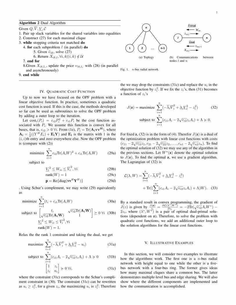
In this section, we will consider two examples to illustratehow the algorithms work. The first one is a n-bus radialnetwork with height equal to one while the other is a five-bus network with a four-bus ring. The former gives ideashow many maximal cliques share a common bus. The latterdemonstrates multiple-level bus and edge sharing. We will alsoshow where the different components are implemented andhow the communication is accomplished.

8

A. n-Bus Radial Network

Consider the topology of the network given in Fig. 1(a). Wehave

M =

M11 0 0 · · · M1n

0 M22 0 · · · M2n

0 0 M33 · · · M3n

......

.... . .

...Mn1 Mn2 Mn3 · · · Mnn

.

1) Primal Algorithm: Eq. (7) becomes

Tr(MW) =

n−1∑l=1

(MHnlWnl +MH

lnWln +MHll Wll)︸ ︷︷ ︸

unique terms

+MHnnWnn.︸ ︷︷ ︸

shared term

Each branch with the end nodes forms a maximal clique. Wehave C = Cl|1 ≤ l ≤ n − 1 where Cl = l, n and U =(n, n). By introducing a slack variable Xnn,l for Wnn to Cl,we have

WClCl=

(Wll Wln

Wnl Xnn,l

).

Let

Ml =

(Mll Mln

Mnl 0

).

Given Wnn, subproblem l for Cl is stated as

minimize Tr(MlWClCl)

subject to V 2l ≤ Tr

(1 00 0

)WClCl

≤ V 2

l

Tr(

0 00 1

)WClCl

= Wnn

WClCl 0

(34)

which is an SDP with a 2 × 2 variable. Recall that φl(Wnn)is the optimal value of subproblem l given Wnn. The masterproblem is

minimize∑n−1l=1 φl(Wnn) +MH

nnWnn

subject to V 2n ≤Wnn ≤ V

2

n.

λnn,l is the Lagrangian multiplier for equality Xnn,l = Wnn

of subproblem l. We update Wnn by

W (t+1)nn = Proj

(W (t)nn − α(t)

(n−1∑l=1

(−λnn,l) +MHnn

))(35)

in [V 2n, V

2

n].In iteration t, bus n broadcasts W (t)

nn to bus l, 1 ≤ l ≤ n−1.After receiving W (t)

nn , For all l, bus l solves its own subproblem(34) by any suitable SDP method, e.g. primal-dual IPM [10],in parallel and then returns λnn,l to bus n.2 After receivingall λnn,l, node n updates Wnn by (35). The communicationpattern is shown in Fig. 1(b).

2For most of the interior-point methods, primal and dual solutions come inpair. When the algorithm finds the optimal WClCl

, it will also give λnn,l.Thus no extra calculation is required to determine λnn,l.

2) Dual Algorithm: Eq. (19) becomes

Tr(MW ) =

n−1∑l=1

(MHnlWnl +MH

lnWln +MHll Wll +

MHnnWnn

n− 1)

As only Wnn is common to all maximal cliques, we haveΩnn = C1, . . . , Cn−1 and

Xnn,1 = Xnn,2 = · · · = Xnn,n−1 = Wnn. (36)

Assume that (36) is arranged as follows. We assign Lagrangianmulipliers to the equalities and we have

υnn,1(Xnn,1 −Xnn,2) = 0

υnn,2(Xnn,1 −Xnn,3) = 0

... (37)υnn,n−2(Xnn,1 −Xnn,n−1) = 0.

For 1 ≤ l ≤ n − 2, Xnn,l(1) = Xnn,1 and Xnn,l(2) =Xnn,l+1. Then we have

υnn,1 = υnn,1 + · · ·+ υnn,n−2,

υnn,l = −υnn,l−1, 2 ≤ l ≤ n− 1.

Let

Ml =

(Mll Mln

Mnl Ml

)where

Ml =

(Mnn

n−1 + υnn,1 + · · ·+ υnn,n−2

), l = 1(

Mnn

n−1 − υnn,l−1

), 2 ≤ l ≤ n− 1

and

WClCl=

(Wll Wln

Wnl Xnn,l

).

Subproblem l is stated as

minimize Tr(MlWClCl)

subject to V 2l ≤ Tr

(1 00 0

)WClCl

≤ V 2

l

V 2n ≤ Tr

(0 00 1

)WClCl

≤ V 2

n

WClCl 0

(38)

which is also an SDP with a 2 × 2 variable. We update theprice by, for 1 ≤ r ≤ n− 2,

υ(t+1)nn,r = υ(t)

nn,r − α(t) (Xnn,r+1 −Xnn,1) . (39)

At time t, node l from Cl, 1 ≤ l ≤ n − 1, solves (38)3,e.g., by IPM, in parallel and sends Xnnl

from the optimalWClCl

to bus n. Whenever any pair of Xnn specified in (47)(e.g., Xnn,1 and Xnn,l for C1 and Cl, respectively) reach busn, price υnn,l−1 can be updated with (39) by bus n and theupdated υnn,l−1 is multicast back to the corresponding buses(e.g., nodes 1 and l). The communication pattern is shown inFig. 1(b).

9

1

2 3

4 5

W22 , W

23

λ 22,1

λ22,2

W44

λ44,3

W22, W

23

λ33,1

λ 33,2

W33

W33

(a) Primal algorithm

1

2 3

4 5

υ 22,1, υ

23,1,

υ 33,1

υ22,1 , υ

23,1 , υ33,1

X 22,1, X

23,1,

X 33,1

X22,2 ,

X23,2 , X

33,2

υ44,1

X44,3

(b) Dual algorithm

Fig. 2. Structure and communication patterns for the five-bus network witha four-bus ring

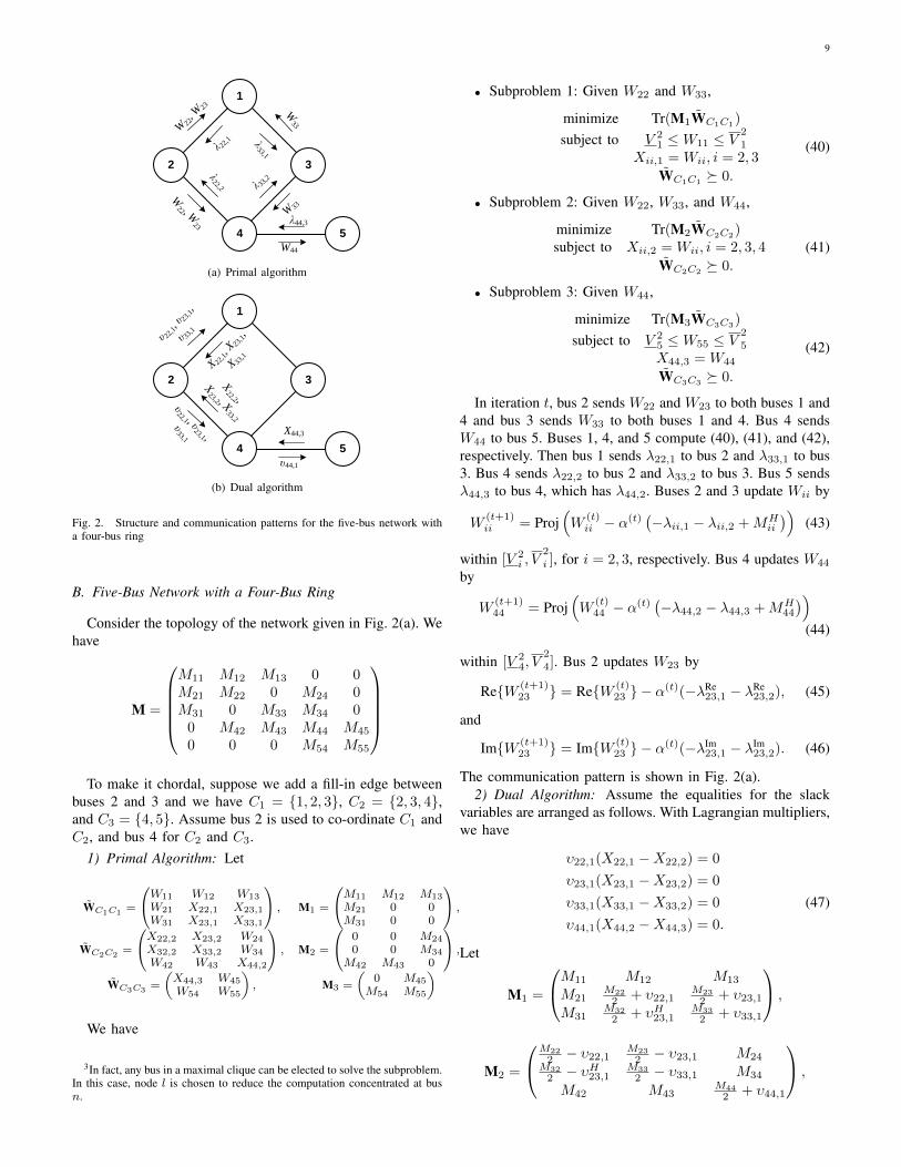
B. Five-Bus Network with a Four-Bus Ring

Consider the topology of the network given in Fig. 2(a). Wehave

M =

M11 M12 M13 0 0M21 M22 0 M24 0M31 0 M33 M34 0

0 M42 M43 M44 M45

0 0 0 M54 M55

To make it chordal, suppose we add a fill-in edge between

buses 2 and 3 and we have C1 = 1, 2, 3, C2 = 2, 3, 4,and C3 = 4, 5. Assume bus 2 is used to co-ordinate C1 andC2, and bus 4 for C2 and C3.

1) Primal Algorithm: Let

WC1C1 =

W11 W12 W13

W21 X22,1 X23,1

W31 X23,1 X33,1

, M1 =

M11 M12 M13

M21 0 0M31 0 0

,

WC2C2=

X22,2 X23,2 W24

X32,2 X33,2 W34

W42 W43 X44,2

, M2 =

0 0 M24

0 0 M34

M42 M43 0

,

WC3C3 =

(X44,3 W45

W54 W55

), M3 =

(0 M45

M54 M55

)

We have

3In fact, any bus in a maximal clique can be elected to solve the subproblem.In this case, node l is chosen to reduce the computation concentrated at busn.

• Subproblem 1: Given W22 and W33,

minimize Tr(M1WC1C1)

subject to V 21 ≤W11 ≤ V

2

1

Xii,1 = Wii, i = 2, 3

WC1C1 0.

(40)

• Subproblem 2: Given W22, W33, and W44,

minimize Tr(M2WC2C2)

subject to Xii,2 = Wii, i = 2, 3, 4

WC2C2 0.

(41)

• Subproblem 3: Given W44,

minimize Tr(M3WC3C3)

subject to V 25 ≤W55 ≤ V

2

5

X44,3 = W44

WC3C3 0.

(42)

In iteration t, bus 2 sends W22 and W23 to both buses 1 and4 and bus 3 sends W33 to both buses 1 and 4. Bus 4 sendsW44 to bus 5. Buses 1, 4, and 5 compute (40), (41), and (42),respectively. Then bus 1 sends λ22,1 to bus 2 and λ33,1 to bus3. Bus 4 sends λ22,2 to bus 2 and λ33,2 to bus 3. Bus 5 sendsλ44,3 to bus 4, which has λ44,2. Buses 2 and 3 update Wii by

W(t+1)ii = Proj

(W

(t)ii − α

(t)(−λii,1 − λii,2 +MH

ii

))(43)

within [V 2i , V

2

i ], for i = 2, 3, respectively. Bus 4 updates W44

by

W(t+1)44 = Proj

(W

(t)44 − α(t)

(−λ44,2 − λ44,3 +MH

44

))(44)

within [V 24, V

2

4]. Bus 2 updates W23 by

ReW (t+1)23 = ReW (t)

23 − α(t)(−λRe23,1 − λRe

23,2), (45)

and

ImW (t+1)23 = ImW (t)

23 − α(t)(−λIm23,1 − λIm

23,2). (46)

The communication pattern is shown in Fig. 2(a).2) Dual Algorithm: Assume the equalities for the slack

variables are arranged as follows. With Lagrangian multipliers,we have

υ22,1(X22,1 −X22,2) = 0

υ23,1(X23,1 −X23,2) = 0

υ33,1(X33,1 −X33,2) = 0 (47)υ44,1(X44,2 −X44,3) = 0.

Let

M1 =

M11 M12 M13

M21M22

2 + υ22,1M23

2 + υ23,1

M31M32

2 + υH23,1M33

2 + υ33,1

,

M2 =

M22

2 − υ22,1M23

2 − υ23,1 M24M32

2 − υH23,1

M33

2 − υ33,1 M34

M42 M43M44

2 + υ44,1

,

10

TABLE INORMALIZED CPU TIME FOR DISTRIBUTION TEST FEEDERSa

Numberof buses Centralized

Cumulative DistributedPrimal Dual Primal Dual

8 1.85 7.21 5.62 1.52 1.0034 298.68 37.79 33.89 1.94 1.70

123 –b 143.39 126.48 2.24 1.64a The CPU times are normalized by 0.0857s.b The solver cannot be applied because of the out-of-memory problem.

and

M3 =

(M44

2 − υ44,1 M45

M54 M55

).

We have• Subproblem 1: Given υ22,1, υ23,1, and υ33,1,

minimize Tr(M1WC1C1)

subject to V 2i ≤Wii ≤ V

2

i , i = 1, 2, 3

WC1C1 0.

(48)

• Subproblem 2: Given υ22,1, υ23,1, υ33,1, and υ44,1,

minimize Tr(M2WC2C2)

subject to V 2i ≤Wii ≤ V

2

i , i = 2, 3, 4

WC2C2 0.

(49)

• Subproblem 3: Given υ44,1,

minimize Tr(M3WC3C3)

subject to V 2i ≤Wii ≤ V

2

i , i = 4, 5

WC3C3 0.

(50)

At time t, bus 2 announces υ22,1, υ23,1, and υ33,1 to buses1 and 4, and bus 4 sends υ44,1 to bus 5. Buses 1, 4, and5 solve (48), (49), and (50), respectively. Then bus 1 sendsX22,1, X23,1, and X33,1 to bus 2. Bus 4 sends X22,2, X23,2,and X33,2 to bus 2. Bus 5 sends X44,3 to bus 4. Bus 2 updatesυ22,1, υ23,1 and υ33,1 by

υ(t+1)ik,1 = υ

(t)ik,1 − α

(t) (Xik,2 −Xik,1) , i, k = 2, 3, i ≤ k,(51)

and bus 4 updates υ44,1 by

υ(t+1)44,1 = υ

(t)44,1 − α(t) (X44,3 −X44,2) . (52)

The communication pattern is shown in Fig. 2(b).

VI. SIMULATION RESULTS

To evaluate the performance of the algorithms, we performextensive simulations on various network settings. Since OPFis formulated as an SDP, the optimal solution can be computedin polynomial time by any popular SDP algorithms, e.g. IPM.Recall that the primal or dual algorithm aims to divide theoriginal problem into smaller ones and to coordinate thesubproblems, which of each can be solved by any SDP solverindependently. The primal and dual algorithms perform coor-dination by indicating what problem data should be allocatedto each subproblem and do simple calculations to update theshared terms (for the primal) and the prices (for the dual).

TABLE IINORMALIZED CPU TIME FOR IEEE POWER TRANSMISSION SYSTEM

BENCHMARKSa

Numberof buses

Centralized Cumulativedual

Distributeddual

iterations Initialstep size

14 5.38 5.38 1.00 1 3030 45.29 58.60 5.38 6 3057 1696.79 49.08 4.28 4 30118 –b 704.46 13.51 9 300a The simulations for this problem set are done on MacBook Pro with 2.4 GHz Intelcore i5 and 4 GB RAM. The CPU times are normalized by 0.1410s.b The solver cannot be applied because of the out-of-memory problem.

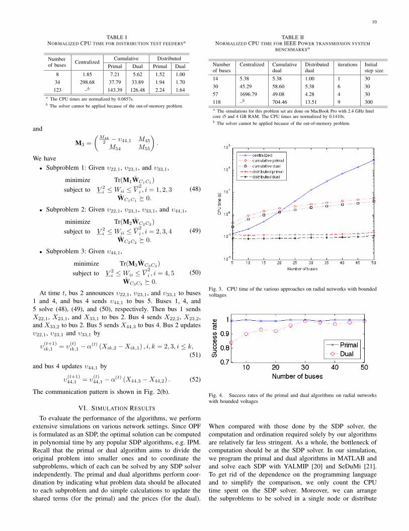
Fig. 3. CPU time of the various approaches on radial networks with boundedvoltages

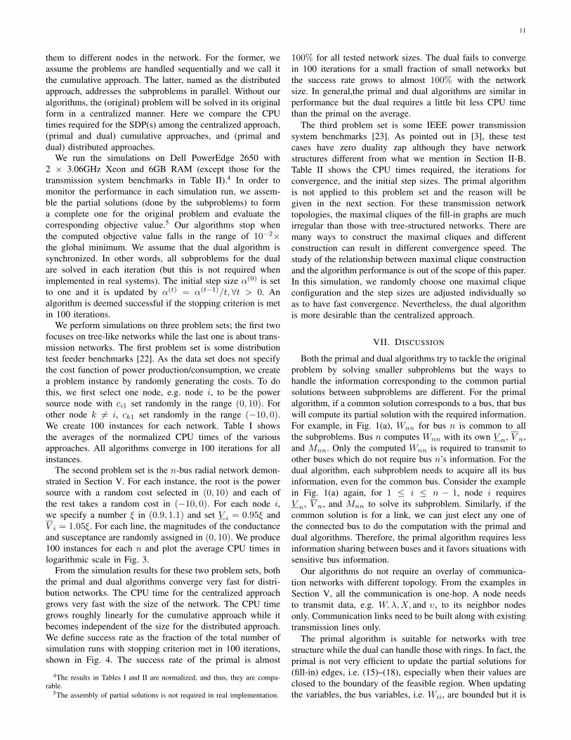
Fig. 4. Success rates of the primal and dual algorithms on radial networkswith bounded voltages

When compared with those done by the SDP solver, thecomputation and ordination required solely by our algorithmsare relatively far less stringent. As a whole, the bottleneck ofcomputation should be at the SDP solver. In our simulation,we program the primal and dual algorithms in MATLAB andand solve each SDP with YALMIP [20] and SeDuMi [21].To get rid of the dependence on the programming languageand to simplify the comparison, we only count the CPUtime spent on the SDP solver. Moreover, we can arrangethe subproblems to be solved in a single node or distribute

11

them to different nodes in the network. For the former, weassume the problems are handled sequentially and we call itthe cumulative approach. The latter, named as the distributedapproach, addresses the subproblems in parallel. Without ouralgorithms, the (original) problem will be solved in its originalform in a centralized manner. Here we compare the CPUtimes required for the SDP(s) among the centralized approach,(primal and dual) cumulative approaches, and (primal anddual) distributed approaches.

We run the simulations on Dell PowerEdge 2650 with2 × 3.06GHz Xeon and 6GB RAM (except those for thetransmission system benchmarks in Table II).4 In order tomonitor the performance in each simulation run, we assem-ble the partial solutions (done by the subproblems) to forma complete one for the original problem and evaluate thecorresponding objective value.5 Our algorithms stop whenthe computed objective value falls in the range of 10−2×the global minimum. We assume that the dual algorithm issynchronized. In other words, all subproblems for the dualare solved in each iteration (but this is not required whenimplemented in real systems). The initial step size α(0) is setto one and it is updated by α(t) = α(t−1)/t, ∀t > 0. Analgorithm is deemed successful if the stopping criterion is metin 100 iterations.

We perform simulations on three problem sets; the first twofocuses on tree-like networks while the last one is about trans-mission networks. The first problem set is some distributiontest feeder benchmarks [22]. As the data set does not specifythe cost function of power production/consumption, we createa problem instance by randomly generating the costs. To dothis, we first select one node, e.g. node i, to be the powersource node with ci1 set randomly in the range (0, 10). Forother node k 6= i, ck1 set randomly in the range (−10, 0).We create 100 instances for each network. Table I showsthe averages of the normalized CPU times of the variousapproaches. All algorithms converge in 100 iterations for allinstances.

The second problem set is the n-bus radial network demon-strated in Section V. For each instance, the root is the powersource with a random cost selected in (0, 10) and each ofthe rest takes a random cost in (−10, 0). For each node i,we specify a number ξ in (0.9, 1.1) and set V i = 0.95ξ andV i = 1.05ξ. For each line, the magnitudes of the conductanceand susceptance are randomly assigned in (0, 10). We produce100 instances for each n and plot the average CPU times inlogarithmic scale in Fig. 3.

From the simulation results for these two problem sets, boththe primal and dual algorithms converge very fast for distri-bution networks. The CPU time for the centralized approachgrows very fast with the size of the network. The CPU timegrows roughly linearly for the cumulative approach while itbecomes independent of the size for the distributed approach.We define success rate as the fraction of the total number ofsimulation runs with stopping criterion met in 100 iterations,shown in Fig. 4. The success rate of the primal is almost

4The results in Tables I and II are normalized, and thus, they are compa-rable.

5The assembly of partial solutions is not required in real implementation.

100% for all tested network sizes. The dual fails to convergein 100 iterations for a small fraction of small networks butthe success rate grows to almost 100% with the networksize. In general,the primal and dual algorithms are similar inperformance but the dual requires a little bit less CPU timethan the primal on the average.

The third problem set is some IEEE power transmissionsystem benchmarks [23]. As pointed out in [3], these testcases have zero duality zap although they have networkstructures different from what we mention in Section II-B.Table II shows the CPU times required, the iterations forconvergence, and the initial step sizes. The primal algorithmis not applied to this problem set and the reason will begiven in the next section. For these transmission networktopologies, the maximal cliques of the fill-in graphs are muchirregular than those with tree-structured networks. There aremany ways to construct the maximal cliques and differentconstruction can result in different convergence speed. Thestudy of the relationship between maximal clique constructionand the algorithm performance is out of the scope of this paper.In this simulation, we randomly choose one maximal cliqueconfiguration and the step sizes are adjusted individually soas to have fast convergence. Nevertheless, the dual algorithmis more desirable than the centralized approach.

VII. DISCUSSION

Both the primal and dual algorithms try to tackle the originalproblem by solving smaller subproblems but the ways tohandle the information corresponding to the common partialsolutions between subproblems are different. For the primalalgorithm, if a common solution corresponds to a bus, that buswill compute its partial solution with the required information.For example, in Fig. 1(a), Wnn for bus n is common to allthe subproblems. Bus n computes Wnn with its own V n, V n,and Mnn. Only the computed Wnn is required to transmit toother buses which do not require bus n’s information. For thedual algorithm, each subproblem needs to acquire all its businformation, even for the common bus. Consider the examplein Fig. 1(a) again, for 1 ≤ i ≤ n − 1, node i requiresV n, V n, and Mnn to solve its subproblem. Similarly, if thecommon solution is for a link, we can just elect any one ofthe connected bus to do the computation with the primal anddual algorithms. Therefore, the primal algorithm requires lessinformation sharing between buses and it favors situations withsensitive bus information.

Our algorithms do not require an overlay of communica-tion networks with different topology. From the examples inSection V, all the communication is one-hop. A node needsto transmit data, e.g. W,λ,X, and υ, to its neighbor nodesonly. Communication links need to be built along with existingtransmission lines only.

The primal algorithm is suitable for networks with treestructure while the dual can handle those with rings. In fact, theprimal is not very efficient to update the partial solutions for(fill-in) edges, i.e. (15)–(18), especially when their values areclosed to the boundary of the feasible region. When updatingthe variables, the bus variables, i.e. Wii, are bounded but it is

12

not the case for the edge variables, i.e. Wik, i 6= k. When thestep size is too large, (15)–(18) may drive the current pointout of the feasible region. If so, the obtained λ cannot beused to form a subgradient, and thus (15)–(18) fail. Whenreaching an infeasible point from a feasible one, we can alwaysstep back and choose a smaller step for an update again.When approaching the optimal solution which is located onthe boundary for SDP, this step-back procedure is not veryefficient. The dual algorithm does not have this problem whenupdating υ with (28). As mentioned, we can always constraina feasible solution by averaging the shared variables.

Tree networks have a very nice property with respect tomaximal clique construction; each branch with its attachednodes form a maximal clique. Hence, it is straightforward todecompose the problem into subproblems. However, when itcomes to a more irregular network like those IEEE transmis-sion system benchmarks, the number of ways to decomposethe problem grows with the size of the network. The perfor-mance of our algorithms also depends on how we form themaximal cliques and the initial step size needs to be adjustedaccordingly. For problems with tree structure, the performanceis easier to predict and the algorithms converge faster.

The dual algorithm is more resistant to communicationdelay than the primal. For the primal, an update of a sharedvariable requires λ from all involved subproblems and thussynchronization is required. Delay of computing or transmit-ting an λ from any subproblem can affect the whole algorithmproceed. On the other hand, an update of an υ requires theX from two pre-associated subproblems according to thearrangement of the inequalities in 22. Delay of computingor transmitting a particular X can affect the update of somebut not all the υ. Thus the dual algorithm is asynchronous.Moreover, we can pair the variables in (22) into equalitiesdifferently and secretly whenever we start the dual algorithm.In some sense, the dual algorithm is more robust to attackstemmed from communication on the communication links.

VIII. CONCLUSION

OPF is very important in planning the schedule of powergeneration. In the smart grid paradigm, more renewable energysources will be incorporated into the system, especially indistribution networks, and the problem size will also growtremendously. As problems with some special structures (e.g.trees for distribution networks) have a zero duality gap, we canfind the optimal solution by solving the convex dual problem.In this paper, we propose the primal and dual algorithms (withrespect to the primal and dual decomposition techniques) tospeed up the computation of the convexified OPF problem.The problem is decomposed into smaller subproblems, eachof which can be solved independently and effectively. Theprimal algorithm coordinates the subproblems by controllingthe shared terms (related to electricity resources) while thedual one manages them by updating the prices. From thesimulation results for tree-structure problems, the computationtime grows linearly with the problem size if we solve thedecomposed problem in a central node with our algorithms.The computation time becomes independent of the problem

size when the subproblems are solved in parallel in differentnodes. Even without nice network structure such as a tree, thedual algorithm outperforms the centralized approach withoutdecomposition. Therefore, the primal and dual algorithms areexcellent in addressing OPF, especially for distribution net-works. In future, we will improve the algorithm by incorporatemore constraints into the OPF problem and move to nonlinearobjective functions.

REFERENCES

[1] P. P. Varaiya, F. F. Wu, and J. W. Bialek, “Smart operation of smartgrid: Risk-limiting dispatch,” Proc. IEEE, vol. 99, pp. 40–57, 2011.

[2] B. Stott, J. Jardim, and O. Alsac, “Dc power flow revisited,” IEEE Trans.Power Syst., vol. 24, pp. 1290–1300, 2009.

[3] J. Lavaei and S. H. Low, “Zero duality gap in optimal power flowproblem,” IEEE Trans. Power Syst., in press.

[4] B. Zhang and D. Tse, “Geometry of feasible injection region of powernetworks,” To appear in proc. Allerton, 2011.

[5] S. Sojoudi and J. Lavaei, “Network topologies guaranteeing zero dualitygap for optimal power flow problem,” Submitted to IEEE Trans. PowerSyst., 2011.

[6] R. A. Jabr, “Radial distribution load flow using conic programming,”IEEE Trans. Power Syst., vol. 21, pp. 1458–1459, 2006.

[7] F. Kelly, A. Maulloo, and D. Tan, “Rate control in communicationnetworks: shadow prices, proportional fairness and stability,” Journalof the Operational Research Society, vol. 49, pp. 237–252, 1998.

[8] D. P. Bertsekas, Nonlinear programming, 2nd ed. Belmont, MA, USA:Athena Scientific, 1999.

[9] M. Chiang, S. H. Low, A. R. Calderbank, and J. C. Doyle, “Layeringas optimization decomposition: A mathematical theory of networkarchitectures,” Proc. IEEE, vol. 95, pp. 255–312, Jan. 2007.

[10] S. Wright, Primal-dual interior-point methods. Philadelphia, PA, USA:Society for Industrial and Applied Mathematics, 1997.

[11] R. E. Tarjan and M. Yannakakis, Simple linear-time algorithms to testchordality of graphs, test acyclicity of hypergraphs, and selectivelyreduce acyclic hypergraphs. Philadelphia, PA, USA: Society forIndustrial and Applied Mathematics, July 1984, vol. 13.

[12] D. R. Fulkerson and O. A. Gross, “Incidence matrices and intervalgraph,” Pacific J. Math., vol. 15, no. 3, pp. 835–855, 1965.

[13] R. E. Neapolitan, Probabilistic reasoning in expert systems: theory andalgorithms. New York, NY, USA: John Wiley & Sons, Inc., 1990.

[14] E. A. Akkoyunlu, “The enumeration of maximal cliques of large graphs,”SIAM Journal on Computing, vol. 2, pp. 1–6, 1973.

[15] K. Nakata, M. Yamashita, K. Fujisawa, and M. Kojima, “A parallelprimal-dual interior-point method for semidefinite programs using pos-itive definite matrix completion,” Parallel Comput., vol. 32, pp. 24–43,Jan. 2006.

[16] M. Fukuda, M. Kojima, K. Murota, and K. Nakata, “Exploiting sparsityin semidefinite programming via matrix completion I: General frame-work,” SIAM J. on Optimization, vol. 11, pp. 647–674, March 2000.

[17] K. Nakata, K. Fujisawa, M. Fukuda, M. Kojima, and K. Murota,“Exploiting sparsity in semidefinite programming via matrix completionII: implementation and numerical results,” Mathematical Programming,vol. 95, pp. 303–327, 2003.

[18] R. Grone, C. R. Johnson, E. M. Sa, and H. Wolkowicz, “Positivedefinite completions of partial hermitian matrices,” Linear Algebra andIts Applications, vol. 58, pp. 109–124, 1984.

[19] S. Boyd and L. Vandenberghe, Convex Optimization. New York, NY,USA: Cambridge University Press, 2004.

[20] J. Lofberg, “YALMIP : A toolbox for modeling and optimizationin MATLAB,” in Proc. International Symposium on Computer AidedControl Systems Design, Sep. 2004, pp. 284–289.

[21] J. F. Sturm, “Using sedumi 1.02, a matlab toolbox for optimization oversymmetric cones,” 1998.

[22] W. H. Kersting, “Radial distribution test feeders,” in Proc. IEEE PowerEngineering Society Winter Meeting, vol. 2, 2001, pp. 908–912.

[23] University of washington, power systems test case archive. [Online].Available: http://www.ee.washington.edu/research/pstca