Distributed Algorithms 6.046J, Spring, 2015

Part 2

Nancy Lynch

1

This Week • Synchronous distributed algorithms:

– Leader Election – Maximal Independent Set – Breadth-First Spanning Trees – Shortest Paths Trees (started)

– Shortest Paths Trees (finish)

• Asynchronous distributed algorithms: – Breadth-First Spanning Trees – Shortest Paths Trees

2

Distributed Networks • Based on undirected graph G = (V, E).

– n = V

– r(u), set of neighbors of vertex u. – deg u = |r u |, number of neighbors of vertex u.

• Associate a process with each graph vertex. • Associate two directed communication channels

with each edge.

3

Synchronous Distributed Algorithms

4

Synchronous Network Model • Processes at graph vertices, communicate using messages. • Each process has output ports, input ports that connect to

communication channels.

• Algorithm executes in synchronous rounds. • In each round:

– Each process sends messages on its ports. – Each message gets put into the channel, delivered to the process

at the other end. – Each process computes a new state based on the arriving

messages.

5

Leader Election

6

n-vertex Clique

• Theorem: There is no algorithm consisting of deterministic, indistinguishable processes that is guaranteed to elect a leader in G.

• Theorem: There is an algorithm consisting of deterministic processes with UIDs that is guaranteed to elect a leader. – 1 round, n2 messages.

• Theorem: There is an algorithm consisting of randomized, indistinguishable processes that eventually elects a leader, with probability 1.

1– Expected time < . 1-€

– With probability > 1 - E, finishes in one round.

7

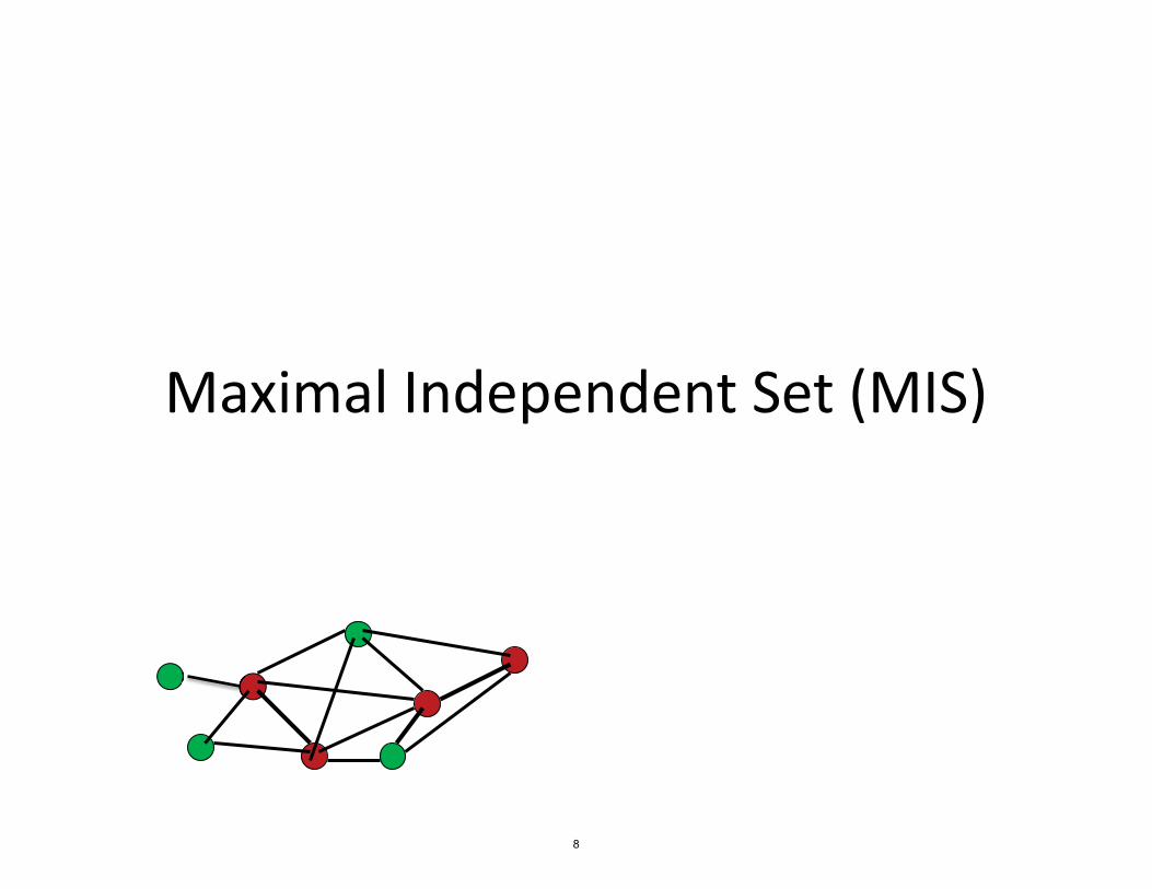
Maximal Independent Set (MIS)

8

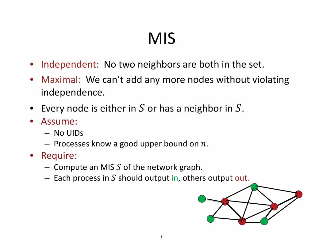
MIS • Independent: No two neighbors are both in the set. • Maximal: We can’t add any more nodes without violating

independence. • Every node is either in S or has a neighbor in S. • Assume:

– No UIDs – Processes know a good upper bound on n.

• Require: – Compute an MIS S of the network graph. – Each process in S should output in, others output out.

9

Luby’s Algorithm • Initially all nodes are active. • At each phase, some active nodes decide to be in, others decide to be

out, the rest continue to the next phase.

• Behavior of active node at a phase: • Round 1:

– Choose a random value r in 1,2, … , n5 , send it to all neighbors. – Receive values from all active neighbors. – If r is strictly greater than all received values, then join the MIS, output in.

• Round 2: – If you joined the MIS, announce it in messages to all (active) neighbors. – If you receive such an announcement, decide not to join the MIS, output out. – If you decided one way or the other at this phase, become inactive.

10

Luby’s Algorithm

• Theorem: If Luby’s algorithm ever terminates, then the final set S is an MIS.

• Theorem: With probability at least 1 - 1

�,all

nodes decide within 4 log n phases.

11

Breadth-First Spanning Trees

12

Breadth-First Spanning Trees • Distinguished vertex va. • Processes must produce a Breadth-First

Spanning Tree rooted at vertex va. • Assume:

– UIDs. – Processes have no knowledge about the graph.

• Output: Each process i = ia should output parent j .

13

Simple BFS Algorithm � Processes mark themselves as they get incorporated into the tree. � Initially, only i

0 is marked.

� Algorithm for process i: � Round 1:

� If i = i0 then process i sends a search message to its neighbors.

� If process i receives a message, then it: � Marks itself. � Selects i

0 as its parent, outputs parent i

� Plans to send at the next round. � Round r > 1:

� If process i planned to send, then it sends a search message to its neighbors.

� If process i is not marked and receives a message, then it: � Marks itself. � Selects one sending neighbor, j, as its parent, outputs parent j . � Plans to send at the next round.

a .

14

Correctness � State variables, per process:

� a,marked, a Boolean, initially true for i false for others � parent, a UID or undefined � a,send, a Boolean, initially true for i false for others � uid

� Invariants: – At the end of r rounds, exactly the processes at distance < r

from v are marked. a

– A process = i has its parent defined iff it is marked. a

– For any process at distance d from va, if its parent is defined, then it is the UID of a process at distance d - 1 from v .a

15

Complexity � Time complexity:

� Number of rounds until all nodes outputs their parentinformation.

� Maximum distance of any node from va, which is < diam

� Message complexity: � Number of messages sent by all processes during the entire

execution. � O( E )

16

Bells and Whistles

• Child pointers: – Send parent/nonparent responses to search

messages. • Distances:

– Piggyback distances on search messages. • Termination:

– Convergecast starting from the leaves. • Applications:

– Message broadcast from the root – Global computation

17

Shortest Paths Trees 1

1

1

1

1

1

1

1

16 12

14 3

4

5

6

18

Shortest Paths • Generalize the BFS problem to allow weights on the graph

edges, weight u,v for edge {u, v} • Connected graph G = V, E , root vertex v , process ia a.

• Processes have UIDs.

• Processes know their neighbors and the weights of their incident edges, but otherwise have no knowledge about the graph.

1

1

1

1

1

1

1

1

16 12

14 3

4

5

6

19

Shortest Paths • Processes must produce a Shortest-Paths Spanning

Tree rooted at vertex va. • Branches are directed paths from va.

– Spanning: Branches reach all vertices. – Shortest paths: The total weight of the tree branch to

each node is the minimum total weight for any path from v in G.a

• Output: Each process i = i should outputaparent j , distance(d), meaning that: – j’s vertex is the parent of i’s vertex on a shortest path

from v ,a– d is the total weight of a shortest path from v to j.a

20

Bellman-Ford Shortest Paths Algorithm � State variables:

� dist, a nonnegative real or 0, representing the shortest known distance from v . Initially 0 for process i , 0 for the others. a a

� parent, a UID or undefined, initially undefined. � uid

� Algorithm for process i: � At each round:

� Send a distance(dist) message to all neighbors. � Receive messages from neighbors; let dj be the distance

received from neighbor j. � Perform a relaxation step: dist : min (dist, min(dj + weight i,j ) .

j

� If dist decreases then set parent : j, where j is any neighbor that produced the new dist.

21

Correctness � Claim: Eventually, every process i has:

� dist = minimum weight of a path from i to i, anda

� if i = ia, parent = the previous node on some shortest path from i to i.a

� Key invariant: – For every r, at the end of r rounds, every process i = i has itsa

dist and parent corresponding to a shortest path from i to ia

among those paths that consist of at most r edges; if there is no such path, then dist = 0 and parent is undefined.

22

Complexity � Time complexity:

� Number of rounds until all the variables stabilize to their final values.

� n - 1 rounds � Message complexity:

� Number of messages sent by all processes during the entireexecution.

� O(n · E )

� More expensive than BFS: � diam rounds, � O E messages

� Q: Does the time bound really depend on n?

23

Child Pointers • Ignore repeated messages. • When process i receives a message that it does not use

to improve dist, it responds with a nonparent message. • When process i receives a message that it uses to

improve dist, it responds with a parent message, and also responds to any previous parent with a nonparent message.

• Process i records nodes from which it receives parent messages in a set children.

• When process i receives a nonparent message from a current child, it removes the sender from its children.

• When process i improves dist, it empties children.

24

Termination • Q: How can the processes learn when the shortest-

paths tree is completed? • Q: How can a process even know when it can output

its own parent and distance?

• If processes knew an upper bound on n, then theycould simply wait until that number of rounds havepassed.

• But what if they don’t know anything about the graph?

• Recall termination for BFS: Used convergecast. • Q: Does that work here?

25

Termination • Q: How can the processes learn when the shortest-

paths tree is completed? • Q: Does convergecast work here? • Yes, but it’s trickier, since the tree structure changes.

• Key ideas: – A process = i can send a done message to its current a

parent after: • It has received responses to all its distance messages, so it

believes it knows who its children are, and • It has received done messages from all of those children.

– The same process may be involved several times in the convergecast, based on improved estimates.

26

100

Termination

100

100

1

1 1 1

1

11

ia 0

1

100

1

1 1 1

1

11

ia

100

1

100

100 0

1

100

100

1

1 1 1

1

11

ia

1

1

51

50

1

505

leaf leaf

27

Asynchronous Distributed Algorithms

28

Asynchronous Network Model • Complications so far:

– Processes act concurrently. – A little nondeterminism.

• Now things get much worse: – No rounds---process steps and message deliveries happen at

arbitrary times, in arbitrary orders. – Processes get out of synch. – Much more nondeterminism.

• Understanding asynchronous distributed algorithms is hard because we can’t understand exactly how they execute.

• Instead, we must understand abstract properties of executions.

29

Aynchronous Network Model • Lynch, Distributed Algorithms, Chapter 8. • Processes at nodes of an undirected graph G = (V, E), communicate using messages.

• Communication channels associated with edges (one in each direction on each edge). – eu,v, channel from vertex u to vertex v.

• Each process has output ports and input ports that connect it to its communication channels.

• Processes need not be distinguishable.

30

Channel Automaton eu,v • Formally, an input/output automaton. • Input actions: send m u,v • Output actions: receive m u,v • State variable:

– mqueue, a FIFO queue, initially empty. • Transitions:

– send m u,v • Effect: add m to mqueue.

– receive m u,v • Precondition: m = head(mqueue) • Effect: remove head of mqueue

eu,v send m u,v receive m u,v

31

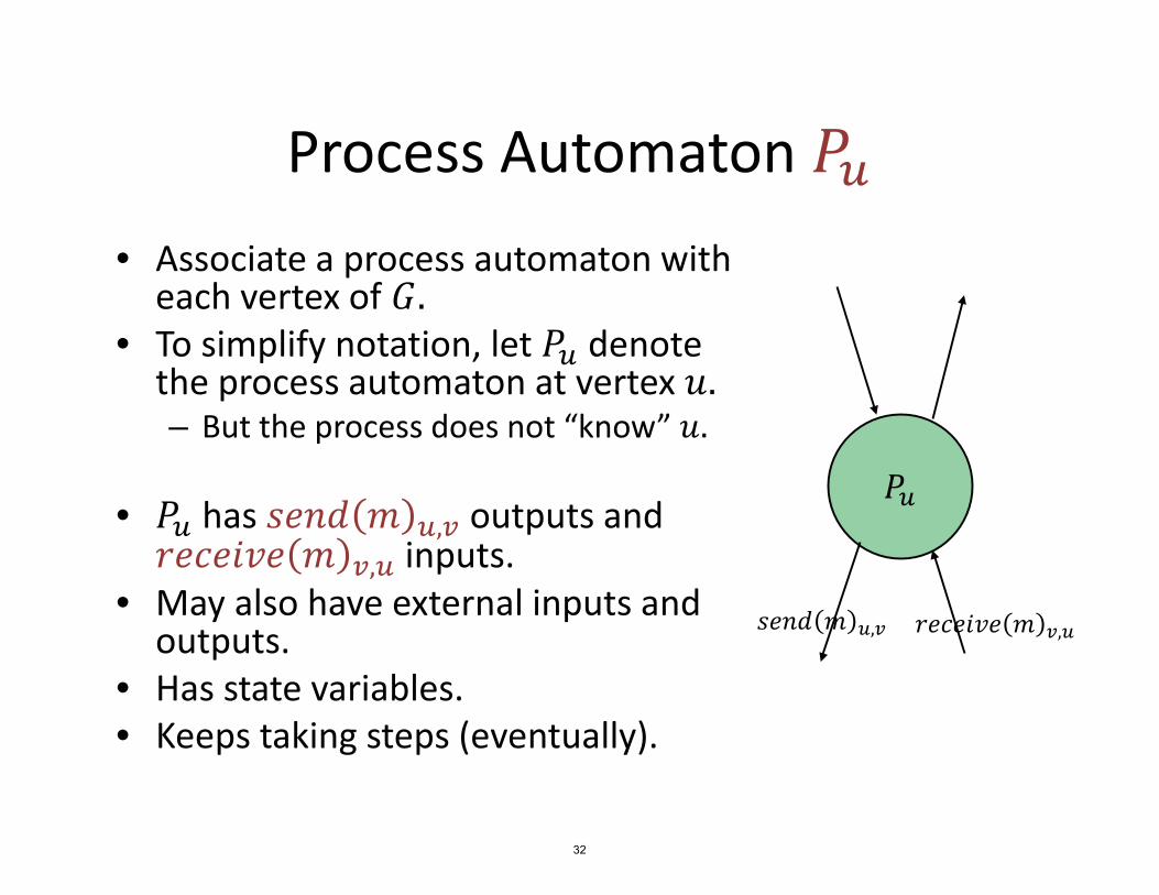
Process Automaton Pu • Associate a process automaton with

each vertex of G. • To simplify notation, let P denote u

the process automaton at vertex u. – But the process does not “know” u.

• P has send m outputs andu u,v receive m inputs.v,u

• May also have external inputs and send m u,v receive

Pu

m v,u outputs. • Has state variables. • Keeps taking steps (eventually).

32

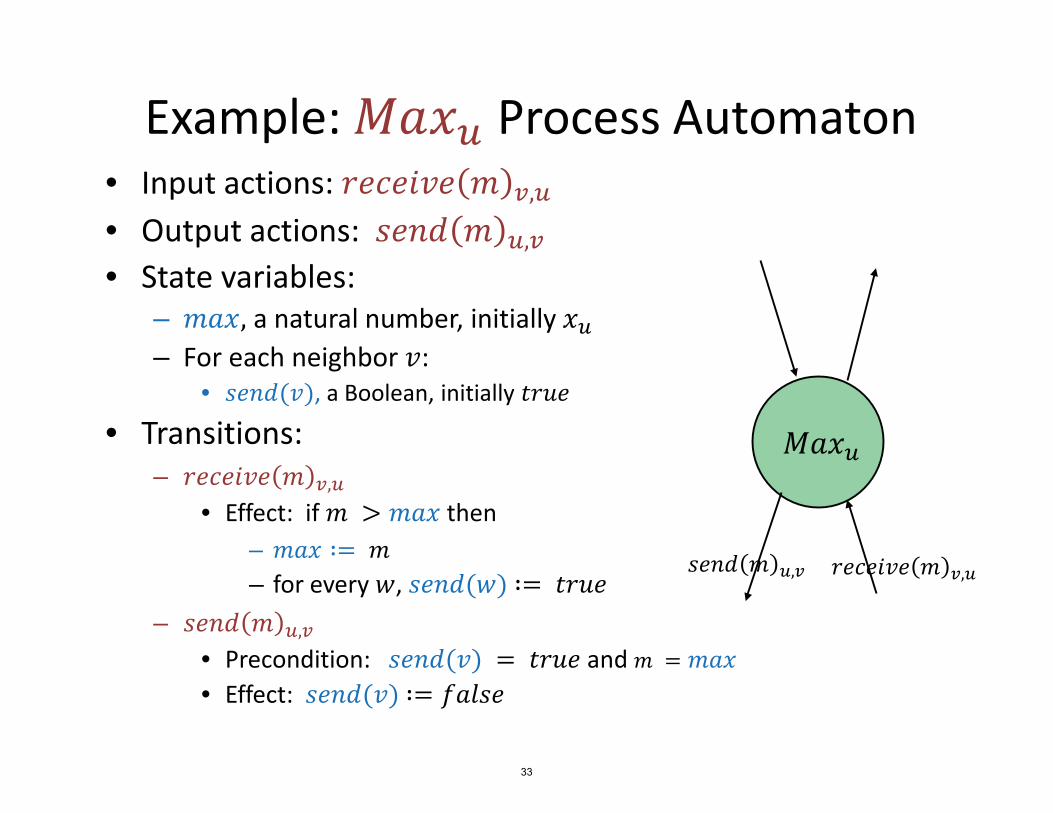
Example: Max Process Automaton u

• Input actions: receive m v,u • Output actions: send m u,v • State variables:

– max, a natural number, initially xu – For each neighbor v:

• send(v), a Boolean, initially true

• Transitions: – receive m v,u

• Effect: if m > max then – max := m

send m u,v receive

Maxu

m v,u – for every w, send(w) := true

– send m u,v • Precondition: send(v) = true and m = max • Effect: send(v) := false

33

Combining Processes and Channels

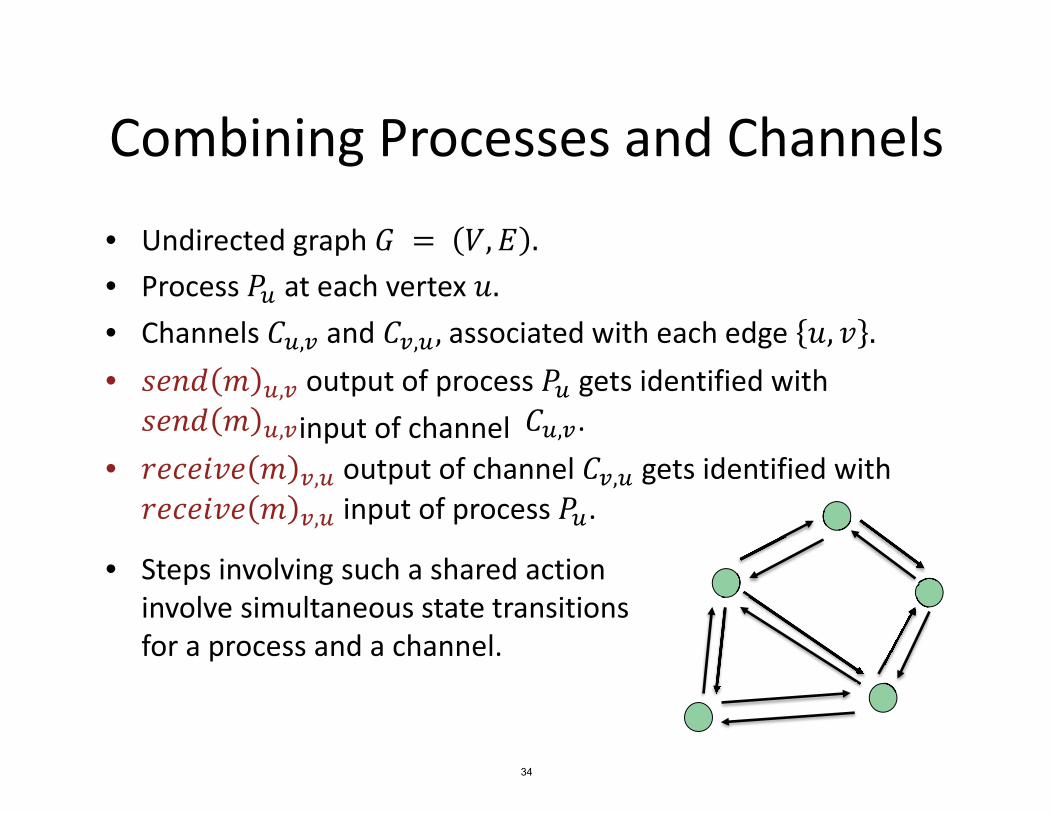
• Undirected graph G = • Process P at each vertex u.u

• Channels e and ev,u, associated with each edge u,v

• send m output of process P gets identified with u,v u

send m input of channel e .u,v u,v

• receive m output of channel e gets identified with v,u v,u

receive m input of process P .v,u u

• Steps involving such a shared action involve simultaneous state transitions for a process and a channel.

V, E .

u, v .

34

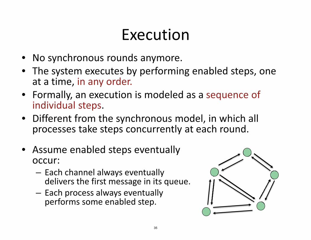
Execution • No synchronous rounds anymore. • The system executes by performing enabled steps, one

at a time, in any order. • Formally, an execution is modeled as a sequence of

individual steps. • Different from the synchronous model, in which all

processes take steps concurrently at each round.

• Assume enabled steps eventually occur: – Each channel always eventually

delivers the first message in its queue. – Each process always eventually

performs some enabled step.

35

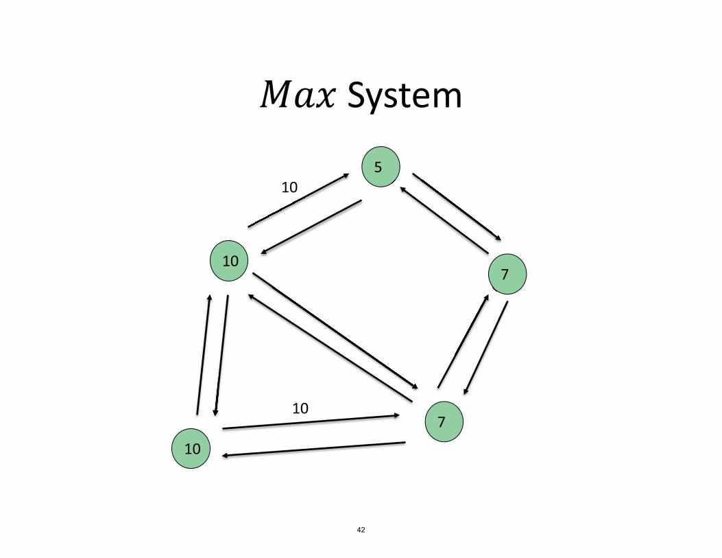
Combining Max Processes and Channels

• Each process Max starts with an initial value xu u.

• They all send out their initial values, and propagate their max values, until everyone has the globally-maximum value.

• Sending and receiving steps can happen in many different orders, but in all cases the global max will eventually arrive everywhere.

36

Max System

5

3

4

10

7

37

Max System

5

3

4

10

7

5

38

Max System

5

3

4

10

7

5

7

39

Max System

5

5

4

10

7

7

10 7

40

Max System

10

5

4

10

7

7

10

7

10

41

Max System

10

5

7

10

7 10

10

42

Max System

10

10

7

10

10

43

Max System

10

10

7

10

10

7

7 10

44

Max System

10

10

10

10

10

45

Complexity � Message complexity:

� Number of messages sent by all processes during the entireexecution.

� O(n · E )

� Time complexity: � Q: What should we measure? � Not obvious, because the various components are taking

steps in arbitrary orders---no “rounds”. � A common approach:

� Assume real-time upper bounds on the time to perform basic steps: � d for a channel to deliver the next message, and � l for a process to perform its next step.

� Infer a real-time upper bound for solving the overall problem.

46

Complexity � Time complexity:

� Assume real-time upper bounds on the time to perform basic steps: � d for a channel to deliver the next message, and � l for a process to perform its next step.

� Infer a real-time upper bound for solving the problem.

� For the Max system: � Ignore local processing time (l = 0), consider only channel

sending time. � Straightforward upper bound: O(diam · n · d)

� Consider the time for the max to reach any particular vertex u, along a shortest path in the graph.

� At worst, it waits in each channel on the path for every other value, which is at most time n · d for that channel.

47

Breadth-First Spanning Trees

48

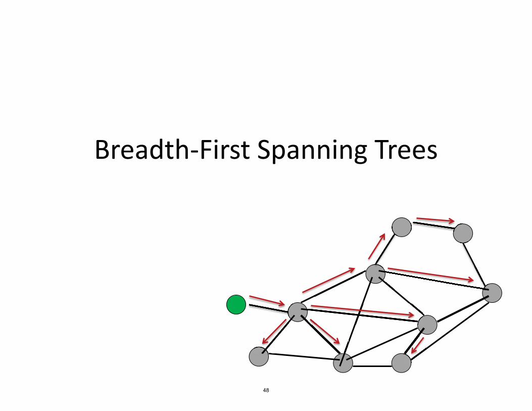
Breadth-First Spanning Trees • Problem: Compute a Breadth-First Spanning Tree in an

asynchronous network. • Connected graph G = (V, E). • Distinguished root vertex v .a• Processes have no knowledge about the graph. • Processes have UIDs

– i is the UID of the root v .a a

– Processes know UIDs of their neighbors, and know which ports are connected to each neighbor.

• Processes must produce a BFS tree rooted at va. • Each process i = i should output parent j , meaninga

that j’s vertex is the parent of i’s vertex in the BFS tree.

49

First Attempt • Just run the simple synchronous BFS algorithm

asynchronously. • Process i sends search messages, which everyone a

propagates the first time they receive it. • Everyone picks the first node from which it receives a search message as its parent.

• Nondeterminism: – No longer any nondeterminism in process decisions. – But plenty of new nondeterminism: orders of message

deliveries and process steps.

50

Process Automaton Pu • Input actions: receive search v,u • Output actions: send search ; parent vu,v u

• State variables: – parent: r u u { 1}, initially 1 – reported: Boolean, initially false – For every v E r u :

• send v E {search, 1}, initially search if u = v , else 1a

• Transitions: –

• Effect: if u = v and parent = 1 thena

– parent := v – for every w, send(w) := search

receive search v,u

51

Process Automaton Pu • Transitions:

–

• Effect: if u = v and parent = 1 thena

– parent := v

– for every w, send(w) := search

–

• Precondition: send(v) = search • Effect: send(v) :1

– parent v u • Precondition: parent = v and reported = false

• Effect: reported : true

receive search v,u

send search u,v

52

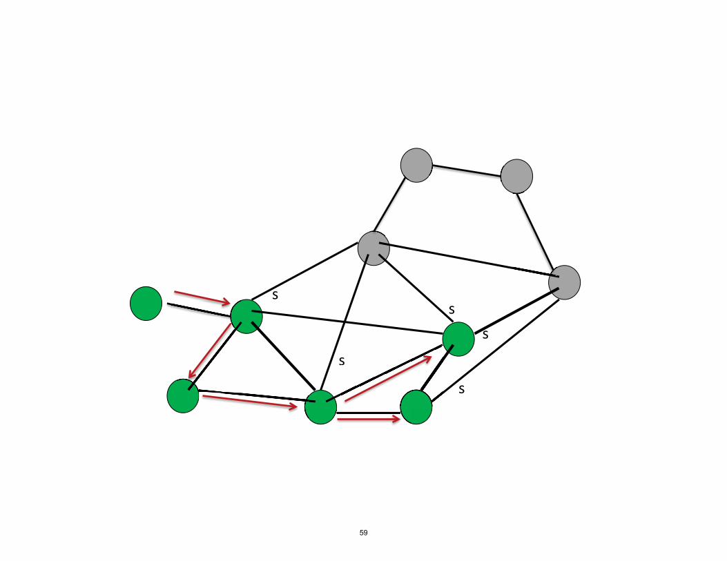
Running Simple BFS Asynchronously

53

54

s

s s s

55

s

s s

s

56

s

s

s s

s

s

57

s

s

s

s s

s

s s

s

s

s s

58

s

s

s

s

s s

59

s s

s

s

ss

s s

s

s

s

60

Final Spanning Tree

61

Actual BFS

62

Anomaly • Paths produced by the algorithm may be

longer than the shortest paths. • Because in asynchronous networks, messages

may propagate faster along longer paths.

63

Complexity � Message complexity:

� Number of messages sent by all processes during the entireexecution.

� O( E )

� Time complexity: � Time until all processes have chosen their parents. � Neglect local processing time. � O( diam · d)

� Q: Why diam, when some of the paths are longer? � The time until a node receives a search message is at most

the time it would take on a shortest path.

64

Extensions • Child pointers:

– As for synchronous BFS. – Everyone who receives a search message sends back a parent or nonparent response.

• Termination: – After a node has received responses to all its search its

messages, it knows who its children are, and knows they are marked.

– The leaves of the tree learn who they are. – Use a convergecast strategy, as before. – Time complexity: After the tree is done, it takes time O(n · d) for the done information to reach ia.

– Message complexity: O(n)

65

Applications

� Message broadcast: - Process i can use the tree (with child pointers) to a

broadcast a message. - Takes O(n · d) time and n messages.

� Global computation: - Suppose every process starts with some initial value,

and process i should determine the value of some a

function of the set of all processes’ values. - Use convergecast on the tree. - Takes O(n · d) time and n messages.

66

Second Attempt

• A relaxation algorithm, like synchronous Bellman-Ford. • Before, we corrected for paths with many hops but low

weights. • Now, instead, correct for errors caused by asynchrony. • Strategy:

– Each process keeps track of the hop distance, changes its parent when it learns of a shorter path, and propagates the improved distances.

– Eventually stabilizes to a breadth-first spanning tree.

67

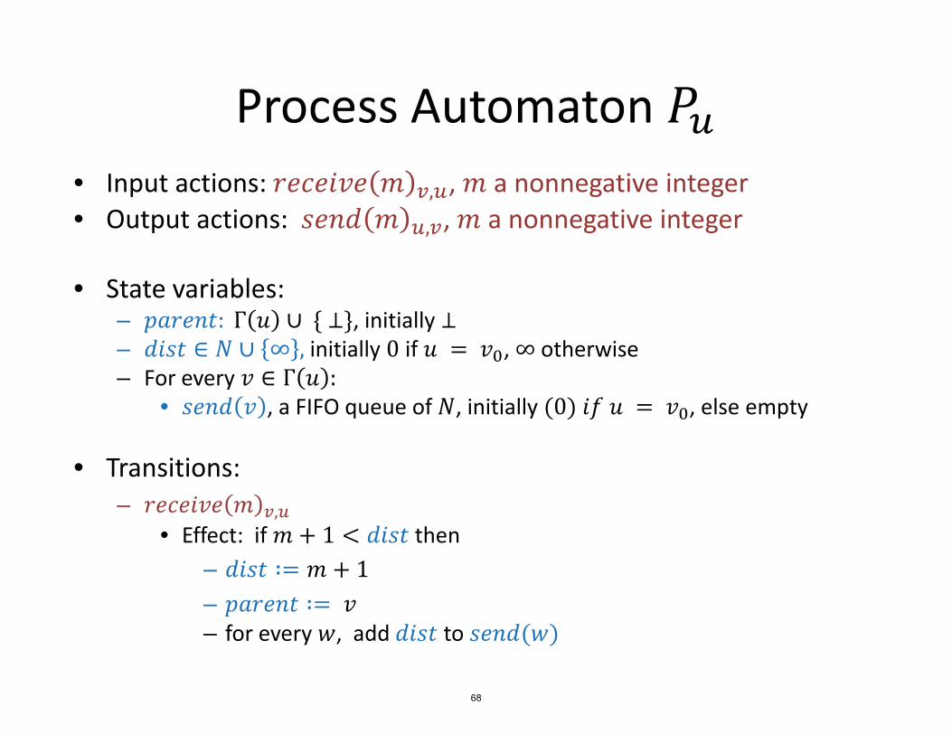
Process Automaton Pu

0 , initially 0 if u = For every v E r u :

v

• Input actions: receive m , m a nonnegative integer v,u

• Output actions: send m , m a nonnegative integer u,v

• State variables: – parent: r u u { 1}, initially 1 – dist E N u v , 0 otherwise a

– • send , a FIFO queue of N, initially (0) if u = v , else empty a

• Transitions: – receive m v,u

• Effect: if m+ 1 < dist then – dist := m + 1

– parent := v – for every w, add dist to send(w)

68

Process Automaton Pu • Transitions:

– receive m v,u • Effect: if m + 1 < dist then

– dist := m + 1

– parent := v

– for every w, add m + 1 to send w – send m u,v

• Precondition: m = head(send v ) • Effect: remove head of send(v)

• No terminating actions…

69

Correctness • For synchronous BFS, we characterized precisely the

situation after r rounds. • We can’t do that now. • Instead, state abstract properties, e.g., invariants and

timing properties, e.g.: • Invariant: At any point, for any node u = v , if itsa

dist = 0, then it is the actual distance on some path from v to u, and its parent is u’s predecessor on such a

a path. • Timing property: For any node u, and any r, 0 < r < diam, if there is an at-most-r-hop path from v to u, then by time r · n · d, node u’s dist is < r. a

70

Complexity � Message complexity:

� Number of messages sent by all processes during the entire execution.

� O(n E )

� Time complexity: � Time until all processes’ dist and parent values have

stabilized. � Neglect local processing time. � O diam · n · d

� Time until each node receives a message along a shortest path, counting time O(n · d) to traverse each link.

71

Termination • Q: How can processes learn when the tree is completed? • Q: How can a process know when it can output its own dist and parent?

• Knowing a bound on n doesn’t help here: can’t use it to count rounds.

• Can use convergecast, as for synchronous Bellman-Ford: – Compute and recompute child pointers. – Process = v sends done to its current parent after: a

• It has received responses to all its messages, so it believes it knows all its children, and

• It has received done messages from all of those children. – The same process may be involved several times, based on

improved estimates.

72

Uses of Breadth-First Spanning Trees

• Same as in synchronous networks, e.g.: – Broadcast a sequence of messages – Global function computation

• Similar costs, but now count time d instead of one round.

73

Shortest Paths Trees

1

1

1

1

1

1

1

1

16 12

14 3

4

5

6

74

Shortest Paths • Problem: Compute a Shortest Paths Spanning Tree in an

asynchronous network. • Connected weighted graph, root vertex v .a• weight u,v for edge u, v . • Processes have no knowledge about the graph, except for

weights of incident edges. • UIDs

• Processes must produce a Shortest Paths spanning tree rooted at va.

• Each process u = v should output its distance and parent ain the tree.

75

Shortest Paths • Use a relaxation algorithm, once again. • Asynchronous Bellman-Ford.

• Now, it handles two kinds of corrections: – Because of long, small-weight paths (as in synchronous

Bellman-Ford). – Because of asynchrony (as in asynchronous Breadth-First

search). • The combination leads to surprisingly high message

and time complexity, much worse than either type of correction alone (exponential).

76

Asynch Bellman-Ford, Process Pu

0 , initially 0 if u = For every v E r u :

v

• Input actions: receive m , m a nonnegative integer v,u

• Output actions: send m , m a nonnegative integer u,v

• State variables: – parent: r u u { 1}, initially 1 – dist E N u v , 0 otherwise a

– • send , a FIFO queue of N, initially (0) if u = v , else empty a

• Transitions: – receive m v,u

• Effect: if m+ weight v,u < dist then – dist := m + weight v,u

– parent := v – for every w, add dist to send(w)

77

Asynch Bellman-Ford, Process Pu • Transitions:

– receive m v,u • Effect: if m+ weight v,u < dist then

– dist := m + weight v,u

– parent := v – for every w, add dist to send(w)

– send m u,v • Precondition: m = head(send v ) • Effect: remove head of send(v)

• No terminating actions…

78

Correctness: Invariants and Timing Properties

• Invariant: At any point, for any node u = v , if itsadist = 0, then it is the actual distance on some path from v to u, and its parent is u’s predecessor on such a path. a

• Timing property: For any node u, and any r, 0 < r < diam, if p is any at-most-r-hop path from v to u, then by atime ???, node u’s dist is < total weight of p.

• Q: What is ??? ? • It depends on how many messages might pile up in a

channel. • This can be a lot!

79

�

Complexity � O(n!) simple paths from v0 to any other node u, which

is O(nn). � So the number of messages sent on any channel is O nn . � nMessage complexity: O E .

� Time complexity: O(nn · n · d).

� Q: Are such exponential bounds really achievable?

21 200

0 0 v -1 v

0 v1

0

0

2k-1

v v v �1 20

2k-2

k

0

80

Complexity � Q: Are such exponential bounds really achievable? � Example:

There is an execution of the network below in which node v�

sends 2k � 2n/2 messages to node vk+1. k

� Message complexity is O(2n/2). � Time complexity is O(2n/2 d).

v -1 v0

v1

0

0

2k-1

v20

2k-2 21

vk

0

0

20

0

0

v �1

81

Complexity • Execution in which node v

k sends 2k messages to node vk+1.

• Possible distance estimates for vk are 2k – 1, 2k – 2,… , 0.

• Moreover, vk can take on all these estimates in sequence: – First, messages traverse upper links, 2k – 1. – Then last lower message arrives at v , 2k – 2. – Then lower message vk-2 � vk-1 arrives, reduces vk-1’s estimate by 2,

message vk-1 � vk arrives on upper links, 2k – 3. – Etc. Count down in binary. – If this happens quickly, get pileup of 2k search messages in e , �1.

v -1v0

v1

0

0

2k-1

v20

2k-2 21

vk

0

0

20

0

0

v �1

82

𝑘

𝑘

Termination • Q: How can processes learn when the tree is

completed? • Q: How can a process know when it can output its own dist and parent?

• Convergecast, once again – Compute and recompute child pointers. – Process = v sends done to its current parent after: a

• It has received responses to all its messages, so it believes it knows all its children, and

• It has received done messages from all of those children. – The same process may be involved several (many) times,

based on improved estimates.

83

Shortest Paths

• Moral: Unrestrained asynchrony can cause problems.

• What to do?

• Find out in 6.852/18.437, Distributed Algorithms!

84

What’s Next? • 6.852/18.437 Distributed Algorithms • Basic grad course • Covers synchronous, asynchronous,

and timing-based algorithms

• Synchronous algorithms: – Leader election – Building various kinds of spanning trees – Maximal Independent Sets and other network structures – Fault tolerance – Fault-tolerant consensus, commit, and related problems

85

Asynchronous Algorithms • Asynchronous network model • Leader election, network structures. • Algorithm design techniques:

– Synchronizers – Logical time – Global snapshots, stable property detection.

• Asynchronous shared-memory model • Mutual exclusion, resource allocation

• Fault tolerance • Fault-tolerant consensus and related problems • Atomic data objects, atomic snapshots • Transformations between models. • Self-stabilizing algorithms

p1

p2

pn

x1

x2

86

And More • Timing-based algorithms

– Models – Revisit some problems – New problems, like clock synchronization.

• Newer work (maybe): – Dynamic network algorithms – Wireless networks – Insect colony algorithms and other biological distributed

algorithms

87

MIT OpenCourseWarehttp://ocw.mit.edu

6.046J / 18.410J Design and Analysis of AlgorithmsSpring 2015

For information about citing these materials or our Terms of Use, visit: http://ocw.mit.edu/terms.