Distinguishing Different Industry Technologies and - AgEcon Search

1

Distinguishing Different Industry Technologies and

Localized Technical Change

Catherine J. Morrison Paul

Department of Agricultural and Resource Economics University of California, Davis [email protected]

Johannes Fritz Sauer

Department of Economics University of Manchester, UK

[email protected]

Selected Paper prepared for Presentation at the Agricultural & Applied Economics Association 2010

AAEA, CAES, & WAEA Joint Annual Meeting, Denver, Colorado, July 25-27, 2010

Copyright 2010 by the authors. All rights reserved. Readers may make verbatim copies of this document for non-commercial purposes by any means, provided that this copyright notice appears on all such copies.

2

Distinguishing Different Industry Technologies and

Localized Technical Change*

Abstract

When different technologies are present in an industry, assuming a homogeneous technology will lead to misleading implications about technical change and inefficient policy recommendations. In this paper a latent class modelling approach and flexible estimation of the production structure is used to distinguish different technologies for a representative sample of E.U. dairy producers, as an industry exhibiting significant structural changes and differences in production systems in the past decades. The model uses a transformation function to recognize multiple outputs; separate technological classes based on multiple characteristics, a flexible generalized linear functional form, a variety of inputs, and random effects to capture firm heterogeneity; and measures of first- and second-order elasticities to represent technical change and biases. We find that if multiple production frontiers are embodied in the data, different firms exhibit different output or input intensities and changes associated with different production systems that are veiled by overall (average) measures. In particular, we find that farms that are larger and more capital intensive experience greater productivity, technical progress and labor savings, and enjoy scale economies that have increased over time.

* This research commenced when the second author was a visiting scholar in the ARE Department at UC Davis. Funding for this research was provided by the British Academy (SG-48134). The authors are grateful to Jakob Vesterlund Olsen, Landscentret, Skejby, Denmark for making the data available. Senior authorship is equally shared. We thank numerous colleagues for comments on an earlier version of this study, including A. Alvarez and L. Orea.

3

Introduction

In most industries different firms operate with different technologies or production systems.

Recognizing these differences is key to understanding structural change, which is likely to involve

varying technical change patterns for different systems or movements toward different systems. That

is, as an industry evolves, technical change does not just increase the amount of output possible from a

given amount of inputs (productivity growth) and induce substitution among inputs (technical change

biases), as is traditionally recognized in productivity analysis. It also involves new production systems

with different characteristics in terms of output and input mix, which may be in the form of a continuum

with discrete changes or may involve entirely different production frontiers.

The presence of different technologies in an industry means that empirical analysis of technical

change, and its drivers and effects, is more complex than is typically modeled by shifts and twists in a

common production frontier or function. In fact, it will be misleading to assume that technology is the

same for different firms, as estimated coefficients of a common technology will be econometrically

biased (Griliches, 1957). This has been recognized in the literature on localized technical change, which

posits differential “drivers” of economic performance depending on the kind of technology used by a

firm (Atkinson and Stigliz, 1969). Modeling and measuring localized technical change in this context

involves first distinguishing the different technologies, and then characterizing the production patterns

associated with these technologies and how they change over time, as we do in this study.1

In particular, the technological specification used for empirical analysis of production

technologies and technical change should accommodate both different points on a production frontier

and separate frontiers for different firms, which we do using a latent class model (LCM) with multiple

1 It also involves productive response to specific factors such as learning by doing and knowledge spillovers that may be technology-specific, which are beyond the scope of this study but will be addressed in subsequent work.

4

characteristics acting as separating variables. We also accommodate firm heterogeneity through firm

random effects and distinguishing two outputs and a variety of inputs.

Recognizing the presence of different output and input mixes and technologies may reduce

apparent substitution elasticities, as substitution possibilities for a specific technology are likely more

limited than implied by a single common production frontier that combines movements within and

between production systems or frontiers. We thus distinguish different technical change patterns,

including the rate of and input biases associated with technical change, using flexible transformation

functions for the different classes that allow for multiple outputs, second-order substitution patterns

and scale economies.

One industry that has exhibited significant structural changes and production system differences

in the past few decades, in both the U.S. and E.U. countries, is the dairy industry. Dairy farms have

experienced a considerable increase in size and reduction in numbers, and have moved toward new

production systems that might be expected to embody different technological characteristics and trends

that we wish to explore. To distinguish farms by their different technologies, researchers have

sometimes categorized producers into, for example, organic versus conventional operations (e.g.,

Kumbhakar et al., 2009). However, such a grouping may be both arbitrary and incomplete. In this study

we instead use our latent class model to group dairy producers into “classes” based on their probability

of having a variety of characteristics (separating variables or q-variables) that proxy different

technologies or production systems.

For example, for dairy operations, one might use characteristics such as cows/hectare or

fodder/cow to proxy the use of pasture or purchased feed (extensive vs. intensive production) and

labor/cow or capital/cow to proxy input intensity (associated with different milking practices). The

latent class model allows us to represent a variety of classes (with the number of classes determined

empirically), based on a combination of differences in such variables as well as multiple netput (output

5

and input) variables. We then use our transformation function model of the production structure to

characterize the technology of the farms in terms of output elasticities for the normalizing output (milk)

that represent input mix, returns to scale, and technical change for each class or group of producers.

The technological differences thus can be summarized by class in terms of summary statistics, estimated

parameters of the underlying multinomial logit (MNL) model, and estimates of the technology.

In particular, class-specific elasticities of the transformation functions with respect to variables

representing technical change indicate the extent to which such factors enhance milk production. As

our focus is on distinguishing productivity growth and input biases for the different technologies, we

represent disembodied technical change by including a time trend as an argument of the transformation

function for each class, with cross-terms for all arguments of the function. We consider which

production systems appear to be the most productive overall, and then evaluate productivity growth

patterns by class through first- and second-order elasticities with respect to the trend term that

measure increased output production given input use and associated input intensity changes.

We also evaluate technical change in terms of, for example, substitutability of chemicals and of

fodder with other inputs. That is, we evaluate the input intensity implications of input biases to

consider trends in chemicals use (and thus environmental issues from leaching and runoff), or use of

purchased feed (and thus environmental issues from intensive production and resulting animal waste).

Additional information about technical change is gained by evaluating returns to scale patterns by

technology, and assessing the extent to which producers switch between classes or production systems.

Specifically, we apply our model to data on Danish dairy farms that are a representative sample

of EU agricultural production and its substantial recent and evolving structural and technological

change. We use our data for 304 farms for 1986-2005, with 3188 observations (an unbalanced panel),

to distinguish the technologies used by these producers and estimate technical change, returns to scale

and substitutability for each group. The separating- or q-variables representing technology differences

6

for these farms in our LCM model include proxies for intensive versus extensive and organic versus

conventional production, input (labor) intensity, and production diversity. Our flexible primal

production structure model with random effects recognizes multiple (milk and non-milk) outputs and

inputs, including separately materials inputs such as chemicals and fodder.

We find that overall average measures do not well reflect individual firms’ production patterns if

the technology of an industry is heterogeneous. That is, we find more than one type of production

frontier embodied in the data, so farms exhibit different technical changes associated with different

production systems, which should be recognized for policy design and implementation. In particular,

larger more capital intensive farms experience greater productivity, technical progress, labor savings,

and scale economies than other farms in our data, and have become more specialized over time,

consistent with trends in the industry toward this type of farm structure.

The Technological Model

For our purposes, a transformation function is desirable for modeling technological processes because

multiple outputs are produced by Danish dairy farms (milk, livestock and crops), precluding estimation

of the production technology by a production function (as in Alvarez and del Corral, 2009), yet we wish

to avoid the disadvantages of normalizing by one input or output, as is required for a distance function.

That is, imposing linear homogeneity on an input (output) distance function requires normalizing the

inputs (outputs) by the input (output) appearing on the left hand side of the estimating equation. This

raises issues not only about what variable should be chosen as the numeraire, but also about

econometric endogeneity because the right hand side variables are expressed as ratios with respect to

the left hand side variable. Although a common approach in input distance function-based agricultural

studies is to normalize by land (e.g., Paul and Nehring, 2005), to express the function in input-per-acre

7

terms, this is questionable when a key issue to be addressed is whether different kinds of farms with

potentially different productivity use land more or less intensively.

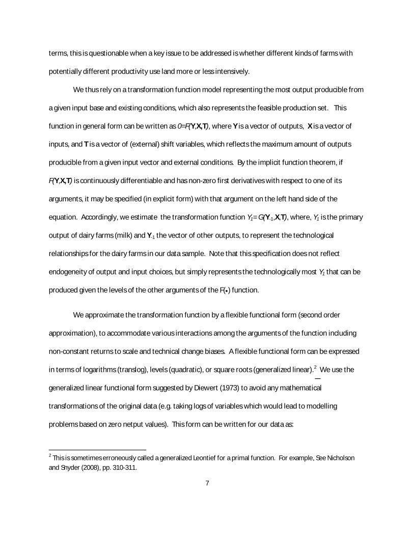
We thus rely on a transformation function model representing the most output producible from

a given input base and existing conditions, which also represents the feasible production set. This

function in general form can be written as 0=F(Y,X,T), where Y is a vector of outputs, X is a vector of

inputs, and T is a vector of (external) shift variables, which reflects the maximum amount of outputs

producible from a given input vector and external conditions. By the implicit function theorem, if

F(Y,X,T) is continuously differentiable and has non-zero first derivatives with respect to one of its

arguments, it may be specified (in explicit form) with that argument on the left hand side of the

equation. Accordingly, we estimate the transformation function Y1= G(Y-1,X,T), where, Y1 is the primary

output of dairy farms (milk) and Y-1 the vector of other outputs, to represent the technological

relationships for the dairy farms in our data sample. Note that this specification does not reflect

endogeneity of output and input choices, but simply represents the technologically most Y1 that can be

produced given the levels of the other arguments of the F( ) function.

We approximate the transformation function by a flexible functional form (second order

approximation), to accommodate various interactions among the arguments of the function including

non-constant returns to scale and technical change biases. A flexible functional form can be expressed

in terms of logarithms (translog), levels (quadratic), or square roots (generalized linear).2 We use the

generalized linear functional form suggested by Diewert (1973) to avoid any mathematical

transformations of the original data (e.g. taking logs of variables which would lead to modelling

problems based on zero netput values). This form can be written for our data as:

2 This is sometimes erroneously called a generalized Leontief for a primal function. For example, See Nicholson and Snyder (2008), pp. 310-311.

8

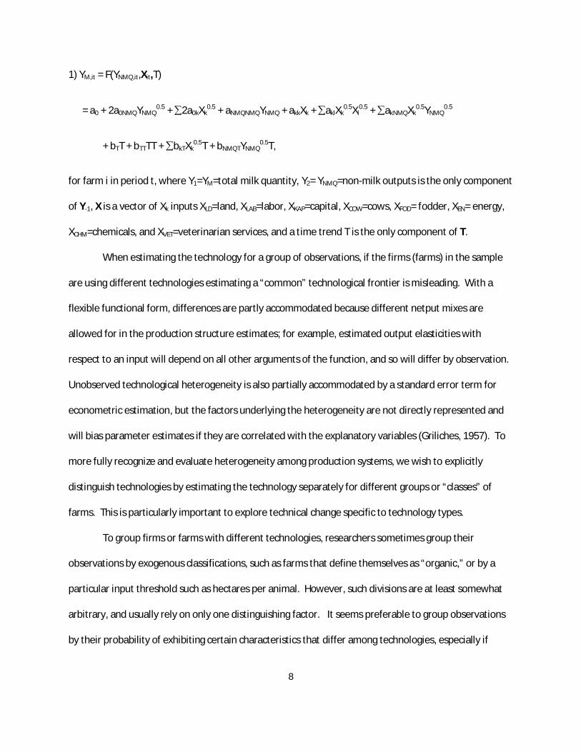
1) YM,it = F(YNMQ,it,Xit,T)

= a0 + 2a0NMQYNMQ0.5 + 2a0kXk

0.5 + aNMQNMQYNMQ + akkXk + aklXk0.5Xl

0.5 + akNMQXk0.5YNMQ

0.5

+ bTT + bTTTT + bkTXk0.5T + bNMQTYNMQ

0.5T,

for farm i in period t, where Y1=YM=total milk quantity, Y2= YNMQ=non-milk outputs is the only component

of Y-1, X is a vector of Xk inputs XLD=land, XLAB=labor, XKAP=capital, XCOW=cows, XFOD= fodder, XEN= energy,

XCHM=chemicals, and XVET=veterinarian services, and a time trend T is the only component of T.

When estimating the technology for a group of observations, if the firms (farms) in the sample

are using different technologies estimating a “common” technological frontier is misleading. With a

flexible functional form, differences are partly accommodated because different netput mixes are

allowed for in the production structure estimates; for example, estimated output elasticities with

respect to an input will depend on all other arguments of the function, and so will differ by observation.

Unobserved technological heterogeneity is also partially accommodated by a standard error term for

econometric estimation, but the factors underlying the heterogeneity are not directly represented and

will bias parameter estimates if they are correlated with the explanatory variables (Griliches, 1957). To

more fully recognize and evaluate heterogeneity among production systems, we wish to explicitly

distinguish technologies by estimating the technology separately for different groups or “classes” of

farms. This is particularly important to explore technical change specific to technology types.

To group firms or farms with different technologies, researchers sometimes group their

observations by exogenous classifications, such as farms that define themselves as “organic,” or by a

particular input threshold such as hectares per animal. However, such divisions are at least somewhat

arbitrary, and usually rely on only one distinguishing factor. It seems preferable to group observations

by their probability of exhibiting certain characteristics that differ among technologies, especially if

9

multiple characteristics may distinguish production systems, as well as to estimate the groups and the

technology together to allow for differences in netput levels and mix. To accomplish this, we combine

the estimation of the production structure with a latent class structure (Greene, 2002, 2005).

The Latent Class Model

Various methods to explicitly allow for heterogeneity in a dairy production model have been used in the

production literature. Some researchers have chosen their data sample based on some criterion of

homogeneous production, such as Tauer and Belbase (1987) who delete farms in their sample with

technologies too different from the norm.3 Some have chosen particular characteristic to divide the

sample and estimate different frontiers, such as location, breed, production process or conventional

versus organic (Hoch, 1962; Bravo-Ureta, 1986; Newman and Matthews, 2006; Tauer, 1998; Kumbhakar

et al., 2009; Gillespie et al., 2009).

Researchers such as Maudos et al. (2002) and Alvarez et al. (2008) accommodate multiple

criteria for separating farms using cluster analysis based on output and input ratios, which divides the

sample according to similarities in specific characteristics by maximizing the variance between groups

and minimizing the variance within groups. Further, Kalirajan and Obwona (1994), Huang (2004), and

Greene (2005) rely on random coefficient models that essentially model each farm as a separate

technology in the form of continuous parameter variation.

It has increasingly been recognized, however, particularly in the stochastic frontier (technical

inefficiency) context that is the focus of most of these studies, that latent class models are desirable for

representing heterogeneity (Greene, 2002, 2005; Orea and Kumbhakar, 2004). This approach separates

3 Tauer and Belbase (1987) deleted dairy farms from their data sample that participated in a particular (dairy diversion) program, that purchased most of their feed or replacement livestock, or that had a large proportion of non-milk sales.

10

the data into multiple technological “classes” according to estimated probabilities of class membership

based on multiple specified characteristics. Each firm/farm can then be assigned to a specific class

based on these probabilities. This method distinguishes the classes based on homogeneity among

firms/farms in terms of both the estimated technological and probability (multinominal logit, MNL)

relationships, rather than looking for similarity in specific variables.

The LCM structure estimates a MNL model together with the estimation of the overall

technological structure (although the number of parameters that may be estimated simultaneously by

LIMDEP is limited by degrees of freedom for multiple output/input specifications). Statistical tests can

be done to choose the number of classes or technologies that should be distinguished. A random

effects model assuming firm-specific random terms along with the technological groupings can be

incorporated to further capture firm heterogeneity, as developed by Greene (2005) and Cameron and

Trivedi (2005) and applied by Abdulai and Tietje (2007) and Alvarez and del Corral (2009). As we focus

on the technological structure and technical change rather than on unobserved “inefficiency,” we do not

include a one-sided error as in a stochastic frontier model. Our specification of multiple technologies

based on multiple characteristics, outputs and inputs, along with random effects and a flexible

functional form, instead accommodates heterogeneity in our sample of Danish dairy farms.

More specifically, we can write the latent class model in general form as equation (1) for class j:

2) YM,it = F(YNMQ,it,Xit,T) j

where j denotes the class or group containing farm i and the vertical bar means a different function for

each class j. As we are assuming that the error term for this function is normally distributed, the

likelihood function for farm i at time t for group j, LFijt, has the standard OLS form. In addition, as in

Greene (2005), the unconditional likelihood function for farm i in group j, LFij, is the product of the

11

likelihood functions in each period t, and the likelihood function for each farm, LFi, is the weighted sum

of the likelihood functions for each group j (with the prior probabilities of class j membership as the

weights): LFi = j Pij LFij.

The prior probabilities Pij are typically parameterized as a multinomial logit (MNL) model, based

on the farm-specific characteristics used to distinguish the technologies or determine the probabilities

of class membership (called separating- or q-variables), qi, and the parameters of the MNL to be

estimated for each class (relative to one group chosen as numeraire), j. That is,

3) Pij = exp( jqi)/[ j exp( jqi)], or,

4) Pij=exp( 0j + n nj qnit)/[ j exp ( 0j + n nj qnit)],

where the qnit are the N q-variables for farm i in time period t.

For our application we include four types of features that are key to distinguishing technologies

and may be represented by alternative ratios.4 One important feature of dairy farms is the intensive or

extensive nature of production, which may be reflected by pasture versus purchased feed; two variables

that could capture this are thus qCOW,HA=cows/hectare and qFOD,COW=fodder/cow. The extent of organic

production may be captured by qCHM,HA=chemicals/hectare or qORG,TOT= organic milk revenue/total

revenue.5 The input intensity of production may be represented by qLABCOW=labor/cow or

4 Variables in levels such as the numbers of cows or hectares could also be included. However, as they are essentially “size” variables that are already included as production structure arguments, and thus are also taken into account in the LCM model, we only included the ratio measures. In preliminary investigation when we did try including such variables, however, their estimated coefficients tended to be quite significant.

5We initially used a organic subsidies/total subsidies variable but it had many missing values as there is only limited information for these categories of farms before 1990, and is also quite highly correlated with the chemicals ratios.

12

qKAP,COW=capital/cow.6 Finally, production diversity or specialization is reflected in the ratio of outputs,

qM,TOT=milk/total output.

We chose our preferred q-variables by trying different combinations of the four types of

indicators and evaluating the latent class model (LCM) q-variable coefficient’s estimates’ significance

and the resulting posterior probabilities for the individual classes. The number of classes is determined

by AIC/SBIC tests suggested by Greene (2002, 2005) that “test down” to show whether fewer classes are

statistically supported. Further, the base model incorporates a panel data specification where each

farm is recognized as a separate entity that is assigned to a particular class:

5) yM,it j = a0 + 2a0NMQ,j yNMQ,it0.5 + 2a0k,j xk,it

0.5 + aNMQNMQ,j yNMQ,it + akk,j xk,it + akl,jxk,it0.5xl.it

0.5 + akNMQ,j xk,it0.5

yNMQ,it0.5 + bT,j tit + bTT,j tittit + bkT,j xk,it

0.5 tit + bNMQT,j yNMQ,it0.5 tit + it j,

for farm i in time period t and class j, with denoting an iid standard error term. However, as an

alternative specification we allow each observation to be a separate entity, allowing farms to switch

between classes to identify changes in production systems over time (i.e. a cross-sectional specification):

6) yM,i j = a0 + 2a0NMQ,j yNMQ,i0.5 + 2a0k,j xk,i

0.5 + aNMQNMQ,j yNMQ,i + akk,j xk,i + akl,jxk,i0.5xl.i

0.5 + akNMQ,j xk,i0.5

yNMQ,i0.5 + bT,j ti + bTT,j titi + bkT,j xk,i

0.5 ti + bNMQT,j yNMQ,i0.5 ti + i j,

for observation i and class j.

The probabilities Pij are therefore functions of the parameters of the MNL model, and the

likelihoods LFij are functions of the parameters of the technology for class j farms, so the likelihood

function for firm i is a function of both these sets of parameters. The overall log-likelihood function for

6 A measure of labor per total output rather than labor per cow was also tried in preliminary estimations.

13

our model, defined as the sum of the individual log-likelihood functions LFi, can be maximized using

standard econometric methods.

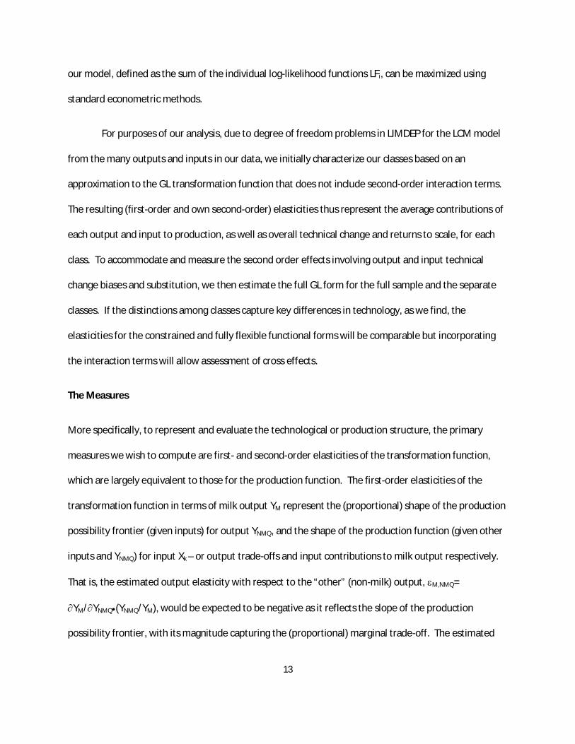
For purposes of our analysis, due to degree of freedom problems in LIMDEP for the LCM model

from the many outputs and inputs in our data, we initially characterize our classes based on an

approximation to the GL transformation function that does not include second-order interaction terms.

The resulting (first-order and own second-order) elasticities thus represent the average contributions of

each output and input to production, as well as overall technical change and returns to scale, for each

class. To accommodate and measure the second order effects involving output and input technical

change biases and substitution, we then estimate the full GL form for the full sample and the separate

classes. If the distinctions among classes capture key differences in technology, as we find, the

elasticities for the constrained and fully flexible functional forms will be comparable but incorporating

the interaction terms will allow assessment of cross effects.

The Measures

More specifically, to represent and evaluate the technological or production structure, the primary

measures we wish to compute are first- and second-order elasticities of the transformation function,

which are largely equivalent to those for the production function. The first-order elasticities of the

transformation function in terms of milk output YM represent the (proportional) shape of the production

possibility frontier (given inputs) for output YNMQ, and the shape of the production function (given other

inputs and YNMQ) for input Xk – or output trade-offs and input contributions to milk output respectively.

That is, the estimated output elasticity with respect to the “other” (non-milk) output, M,NMQ=

YM/ YNMQ (YNMQ/YM), would be expected to be negative as it reflects the slope of the production

possibility frontier, with its magnitude capturing the (proportional) marginal trade-off. The estimated

14

output elasticity with respect to input k, M,k= YM/ Xk (Xk/YM), would be expected to be positive, with its

magnitude representing the (proportional) marginal productivity of Xk.

Second-order own-elasticities may be computed to confirm that the curvature of these

functions satisfies regularity conditions; the marginal productivity would be expected to be increasing at

a decreasing rate, and the output trade-off decreasing at an increasing rate, so second derivatives with

respect to both YNMQ and Xk would be negative (concavity with respect to both outputs and inputs).

Returns to scale may be computed as a combination of the YM elasticities with respect to the

non-milk output(s) and inputs. For example, for a production function returns to scale is defined as the

sum of the input elasticities. Similarly for a transformation function such a measure must control for the

other output(s). Formally, returns to scale are defined for the transformation function similarly to the

treatment for the distance function in Caves, Christensen and Diewert (1982) – for our purposes as

M,X= k M,k M,NMQ).7

Technical change is measured by shifts in the overall production frontier over time. As our only

technical change variable is the trend term T, productivity/technical change is estimated as the output

elasticity with respect to T, M,T= lnYM/ T= YM/ T (1/YM). This represents how much more milk may be

produced on an annual basis in proportional terms, given the levels of the inputs and other output(s).

These measures may be computed for each observation and presented as a averages over a

subset of observations (such as for the full sample, a farm, a time period or a particular class), or may be

7 The adaptation of this treatment for the transformation function was outlined by W. Erwin Diewert in private correspondence. Essentially, given the transformation function defined in equation (1), if all inputs are increased by a scale factor S, and one looks for another scalar factor (US) such that U times the initial vector of outputs Y is still on the transformation function, U(S) is implicitly defined by: U(S)Y1=F(U(S)Y2,SX,T). The implicit function rule

can then be used to calculate the derivative U’(S) evaluated at S=1: U’(1) = ( kdlnF(Y2,X)/dlnXk)/(1-dlnF(Y2,X)/dlnY2). If this measure exceeds one, it implies increasing returns to scale.

15

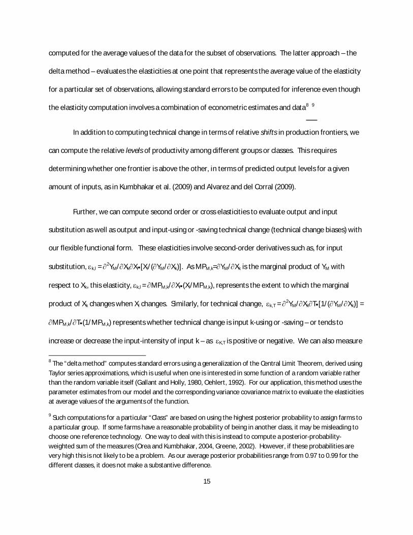
computed for the average values of the data for the subset of observations. The latter approach – the

delta method – evaluates the elasticities at one point that represents the average value of the elasticity

for a particular set of observations, allowing standard errors to be computed for inference even though

the elasticity computation involves a combination of econometric estimates and data8 9

In addition to computing technical change in terms of relative shifts in production frontiers, we

can compute the relative levels of productivity among different groups or classes. This requires

determining whether one frontier is above the other, in terms of predicted output levels for a given

amount of inputs, as in Kumbhakar et al. (2009) and Alvarez and del Corral (2009).

Further, we can compute second order or cross elasticities to evaluate output and input

substitution as well as output and input-using or -saving technical change (technical change biases) with

our flexible functional form. These elasticities involve second-order derivatives such as, for input

substitution, k,l = 2YM/ Xk Xl [Xl/( YM/ Xk)]. As MPM,k= YM/ Xk is the marginal product of YM with

respect to Xk, this elasticity, k,l = MPM,k/ Xl (Xl/MPM,k), represents the extent to which the marginal

product of Xk changes when Xl changes. Similarly, for technical change, k,T = 2YM/ Xk T [1/( YM/ Xk)] =

MPM,k/ T (1/MPM,k) represents whether technical change is input k-using or -saving – or tends to

increase or decrease the input-intensity of input k – as K,T is positive or negative. We can also measure

8 The “delta method” computes standard errors using a generalization of the Central Limit Theorem, derived using Taylor series approximations, which is useful when one is interested in some function of a random variable rather than the random variable itself (Gallant and Holly, 1980, Oehlert, 1992). For our application, this method uses the parameter estimates from our model and the corresponding variance covariance matrix to evaluate the elasticities at average values of the arguments of the function.

9 Such computations for a particular “Class” are based on using the highest posterior probability to assign farms to a particular group. If some farms have a reasonable probability of being in another class, it may be misleading to choose one reference technology. One way to deal with this is instead to compute a posterior-probability-weighted sum of the measures (Orea and Kumbhakar, 2004, Greene, 2002). However, if these probabilities are very high this is not likely to be a problem. As our average posterior probabilities range from 0.97 to 0.99 for the different classes, it does not make a substantive difference.

16

whether returns to scale are increasing or decreasing over time (with technical change) for each class by

computing Y,X,T= Y,X/ T.

The Data

The Danish dairy sector is undergoing a strong restructuring where the traditional farm model – herds of

about 40 tied-up cows based on grazing – rapidly is disappearing. It is being replaced by another model

which emphasizes larger herds (100 to 120 cows) in loose-housing systems with cubicles, based on

mixed feed and fodder.

Danish dairy farms have on average a herd of 94 cows for an agricultural area of 95 hectares,

and with a national milk quota of about 4.5 million tons provide approximately 3% of the milk

production of the European Union (EU 27). In comparison to other European countries, Danish dairy

farms are characterized by very high labor productivity (Perrot et al 2007); for example, in 2005 5,900

Danish dairy farms, mainly located in Jutland (the West border of the country), produced as much milk

as the French region Brittany where there are three times as many producers. Along with Spain and Italy

(where farms remain, however, much smaller), restructuring of the Danish dairy sector has been the

most spectacular in the EU: the herd size has doubled during the last ten years (from 45 cows in 1995)

and the number of farms correspondingly halved. The mean annual milk production per farm reached

850,000 kg in 2006, a record level in the EU (Perrot et al. 2007).

Our data are for 304 Danish dairy farms for 1986-2005, with 3188 observations. The data used

for our empirical investigation are for milk (total and organic) and non-milk outputs, and land, labor,

capital, cow, fodder, energy, veterinary and chemicals inputs, as well as deflators (producer price

indexes for milk and dairy products, agricultural materials, and machinery and buildings). The data are

taken from Landscentret, Denmark (“Regnskabsdatabase”: an economic farm account database

17

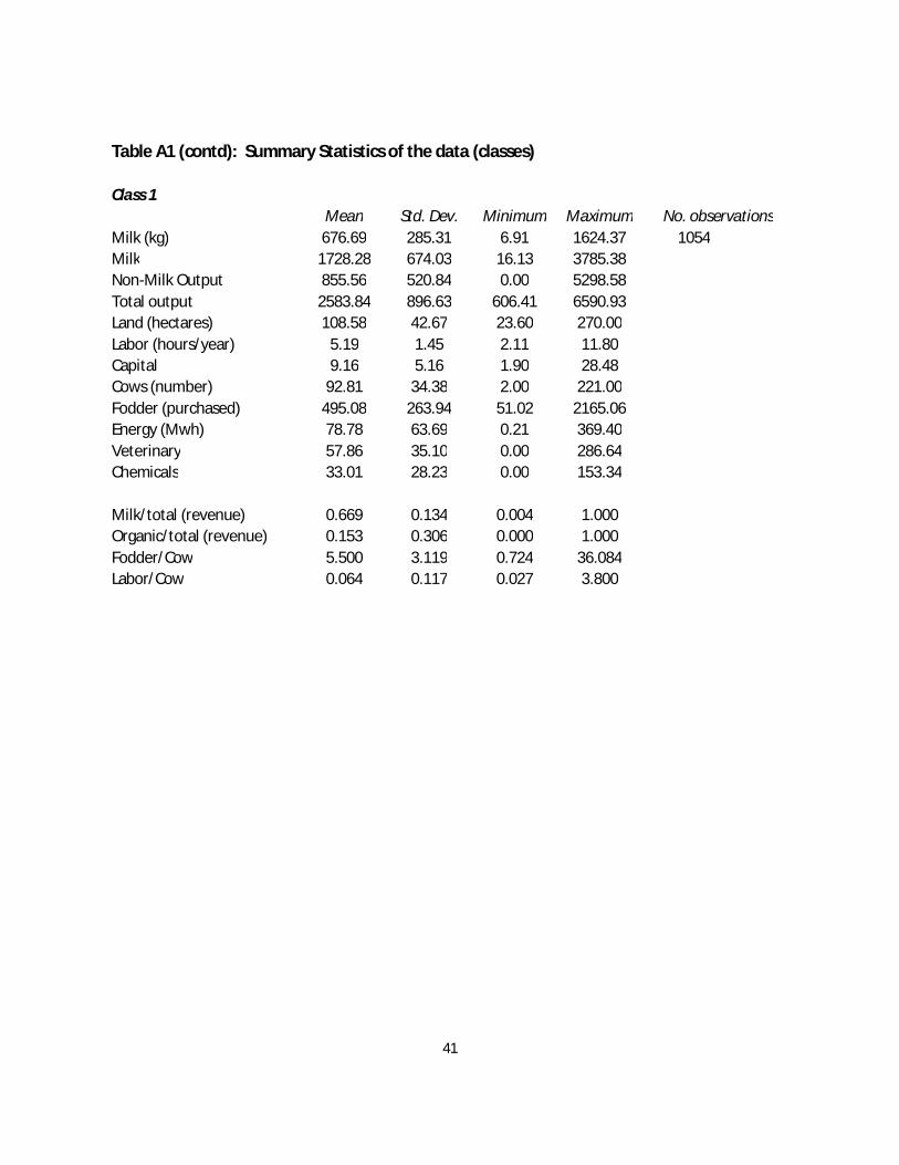
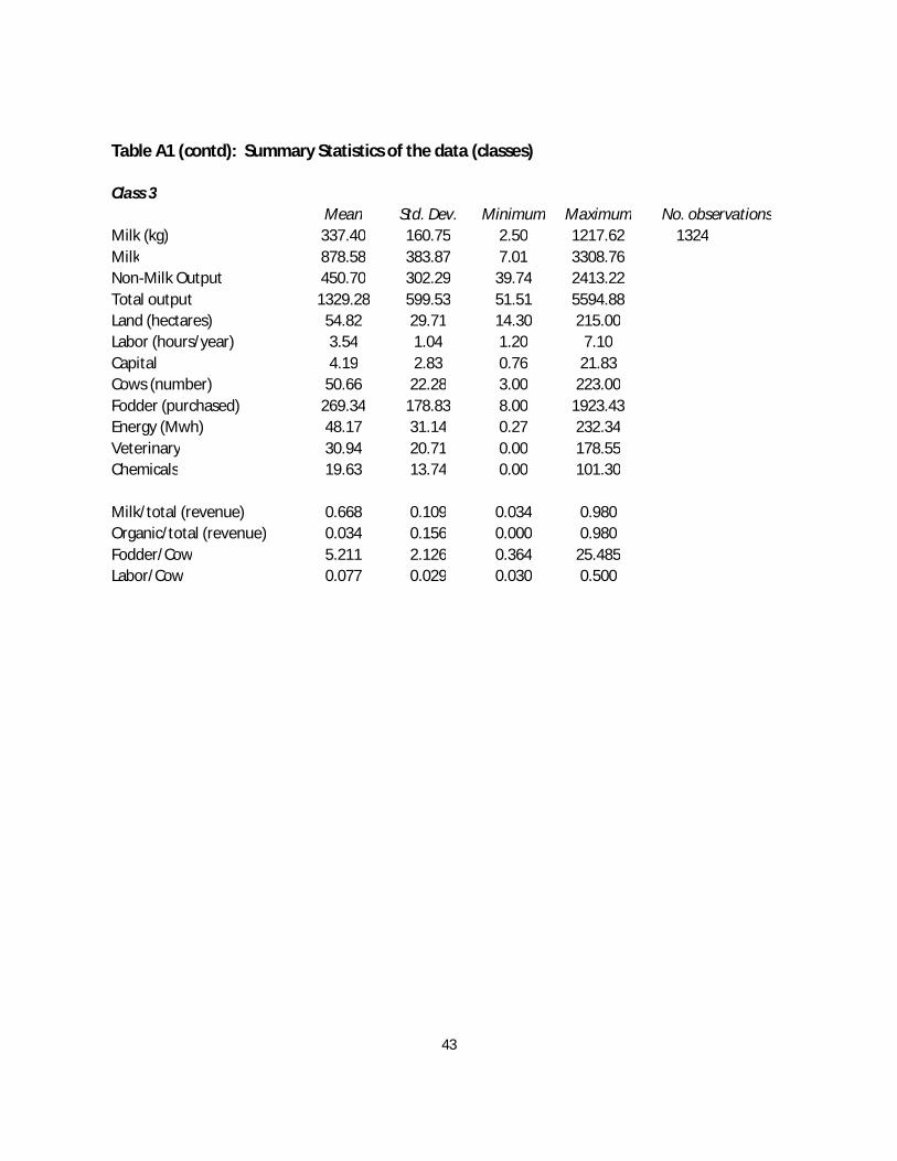
collected for various years) and Danmark Statistic (various agricultural price indexes). Summary

statistics for the data overall, and by the final preferred (3) classes and for the first and last years of our

data sample are presented in Appendix Table A1.

Overall, milk was about two-thirds of total production for these farms, which averaged about 77

hectares with about 68 cows, 4300 labor hours/year, 6.2 million Danish Kronor in capital, and about

5600 Kronor in feed/cow/year, with revenue of about 1,800,000 Kronor/year (in 1986 monetary units).

When divided into classes (as discussed below), class 1 farms tend to be larger operations with about

2,500,000 Kroner/year in revenue, more cows and land (about 93 cows and 109 hectares), less labor and

more capital input per cow, and more organic production and fodder/cow on average – although the

range for all of the variables is very large. Class 3 is the reverse – seemingly more traditional farms that

are smaller, somewhat more diversified, with more labor and less land, capital and fodder per cow.

Class 2 is in the middle in terms of size, with the least milk/total revenue (more diversification) and

organic/total production.

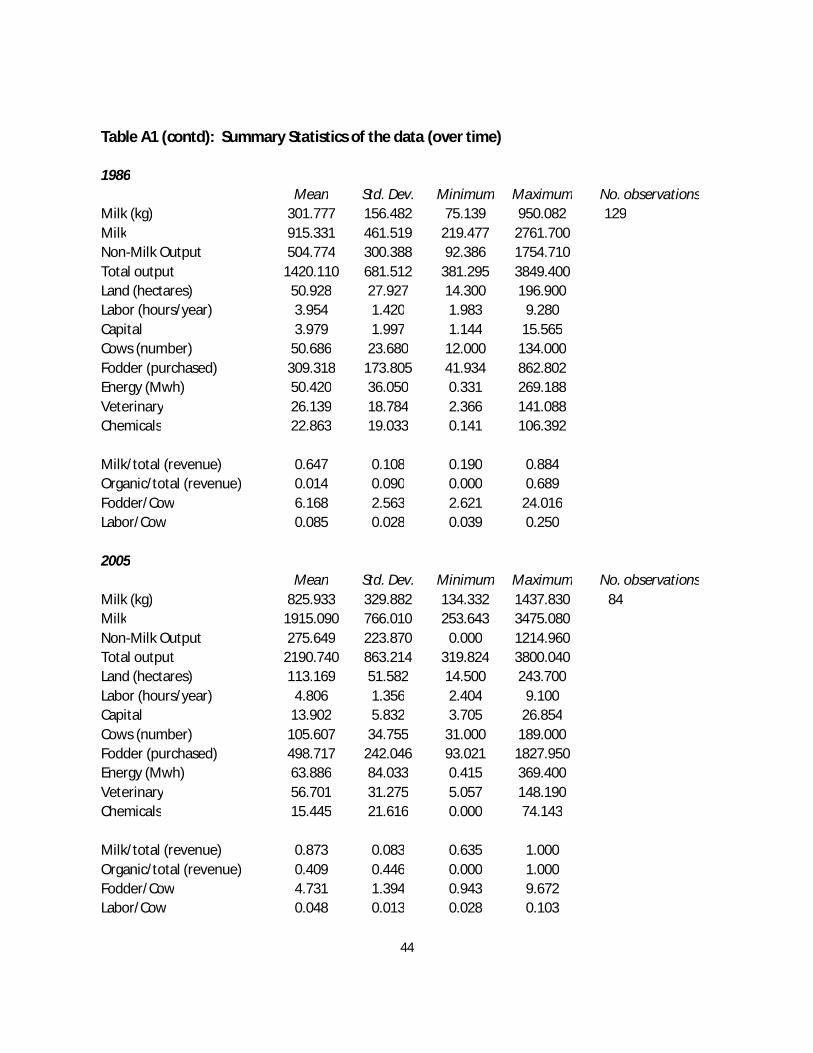
Differences over time for the data for the first and last years of the sample show a dramatic

increase in milk production per farm (nearly three-fold) and proportion of organic milk while non-milk

output was dropping, combined with much more capital and land, less chemicals use, more than twice

as many cows per farm, and less labor and fodder per cow. These trends are consistent with those for

dairy farms in other EU countries and especially the U.S. toward larger more specialized farms and more

capital-intensive production systems.

The Results

We estimated our LCM model by Maximum Likelihood (ML) methods using LIMDEP 9.0. As noted, our

base production structure model includes all first order and own second order terms, but it does not

18

include cross-terms between outputs and inputs as there were too many parameters to distinguish

classes with the fully flexible model in the LIMDEP algorithm. The first-order elasticities representing

output and input composition and technical change would be expected, however, to be well

approximated by such estimates (as we will see below), so the fundamental characteristics of the

different farms are taken into account for the separation of the farms into classes.

The parameter estimates for this production structure model are presented in the first panel of

Appendix Table A2 for the full sample.10 As discussed above, however, the measures of interest for our

analysis are computed as combinations of these parameters. The first measures to evaluate are thus

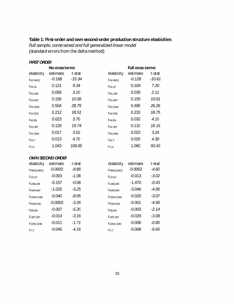
the elasticity measures presented in the first panel of Table 1 for the full data sample. These first order

output (milk, YM) elasticity estimates reflect output tradeoffs, input contributions, returns to scale and

technical change, evaluated at the mean values of the variables for all farms in our data.

(table 1)

The (proportional) tradeoffs between the outputs are given by the M,NMQ elasticity, where M

and NMQ denote YM and YNMQ. The estimate for this elasticity of approximately -0.17 shows that

producing one percent more milk, given input use, on average involves about 17 percent less “other”

outputs for the farms in our data. The (proportional) productive contributions of the inputs are given by

the M,k elasticities (k= LD, LAB, KAP, COW, FOD, EN, VET, CHM). These output elasticities with respect to

the inputs show that livestock (XCOW) comprises the largest marginal input “share” or contribution to

output at about 50 percent, fodder is about 21 percent, capital is next at about 16 percent, and land and

veterinary care follow at about 12-13 percent. Labor has a small productive contribution of about 6

percent, and chemicals and energy even less at about 2 percent. In combination, these estimates result 10 We did not provide all the estimates for all the classes as the elasticities rather than the parameter estimates are our primary results to analyze. However, the full set of estimates is available from the authors upon request.

19

in a slightly increasing returns to scale ( Y,X) estimate of 1.04; a one percent increase in all netputs

generates an increase in milk production of about 1.04 percent.

In turn, our technical change measure presented in the first panel of Table 1, reflecting changes

in potential output (milk) production over time holding input use and non-milk production constant, is

statistically as well as economically significant at about 0.013; on average milk output per unit of input

has increased about 1.3 percent per year for the farms in our sample. Note also that second order own-

elasticity estimates confirm the appropriate curvature on the relationships represented by the first

order output elasticities; as non-milk production YNMQ increases the opportunity cost in terms of milk

production increases on the margin, and the (proportional) marginal products of all inputs are (positive

but) diminishing. The rate of technical change is also decreasing over time.

A fundamental premise of our study, however, is that such overall (average) measures over the

whole sample do not well reflect individual firms’/farms’ production patterns if the technology is

heterogeneous. That is, if there is more than one type of production frontier embodied in the data, it

should be recognized that different farms may exhibit different output or input intensities and changes

associated with different production systems.

To distinguish and evaluate such technologies and associated technical change, we needed to

specify the q- or separating-variables underlying the different technologies, and determine the number

of different technologies or classes in which to group our data. For the first of these problems, we used

different combinations of possible variables reflecting four distinctions among farm technologies we

believe to be important for dairy farms – extensive/intensive, organic/conventional, input (labor and

capital) intensity, and diversification/specialization. Although the models using different subsets of

these potential q-variables are not nested and thus cannot be directly tested, we evaluated their

20

relevance based on the significance of the resulting MNL coefficient ( nj) estimates. These experiments

suggested that the empirically most relevant variables for grouping were qFOD,COW=fodder/cow, qORG,TOT=

organic revenue/total revenue, qLAB,COW=labor/cow and qM,TOT=milk/total output.

(table 2)

To determine how many classes are statistically supported, it is now recognized in the literature

that one should “test down” from the most classes to determine whether restricting classes is justified

by statistical tests. Although likelihood ratio tests may be used, Greene (2005) showed that it is

preferable to use AIC and SBIC tests – in this case to test down from four classes. Such tests showed for

our specification that three classes were statistically supported but two classes were not.

The o and n estimates for this model are presented in Table 2. All of the constant terms are

statistically significant at the 1 percent level, suggesting that even without the q-variables the different

farm production structures show significantly distinct technologies. However, the q-variables identify

additional separating characteristics. Also note that the prior probabilities for our preferred three class

model are about 0.39. 0.08 and 0.54 for classes 1-3 but the average posterior probabilities for the farms

within each of these classes are about 0.99, 0.97 and 0.98 (for the 110, 74 and 120 farms in those

categories), respectively, indicating a very good “fit” for our classification scheme.

A primary distinguishing factor among these farms – in terms of statistical significance – appears

to be the amount of milk relative to total output. For our three class model, Class 3 becomes the base

class with the highest prior probability, and the estimated parameters show that farms in other classes

have a lower milk share, holding all else constant, although summary statistics show a slightly lower milk

share for Class 3 overall. Farms in both Class 1 and Class 2 also use less labor/cow than those in Class 3,

21

and those in Class 1 sell relatively more organic milk and in Class 2 (with a less than 10 percent prior

probability of being in this class) purchase less fodder/cow, as evident from the summary statistics.

Given the division of classes into three groups based on the chosen q-variables and first order

technological specification, the next step is representing the full production technology for the separate

classes to identify substitution patterns. First, to evaluate the desirability of including additional cross-

terms, as well as the appropriateness of using the base constrained (first order) model for distinguishing

the classes, we estimated a fully flexible version of equation (1) for comparison. The parameter

estimates for this model are presented in the second panel of Appendix Table A1, and the first order and

own second order elasticities in the second panel of Table 1. Tests of the joint significance of the cross-

effects relative to constraining them to zero showed that a fully flexible form is statistically supported.11

For our full analysis of the production structure, therefore, we wish to use the fully flexible model.

Although degrees of freedom problems with the LIMDEP LCM algorithm precludes using such a

model for the first step, the validity of using the base model for distinguishing classes but the flexible

model for evaluating the full production structure may be inferred by comparing the elasticities for the

constrained and unconstrained models from Table 1. Such a comparison shows that, although the cross-

terms will provide us with additional insights about underlying substitution relationships, the overall

netput composition patterns are effectively captured by the constrained model.

In particular, although the first order input elasticities for land and labor are somewhat smaller

when interactions among the other arguments of the function are allowed for, they are roughly within

two standard deviations of each other and the remaining elasticities are statistically equivalent. The

most substantial differences are the technical change term that is nearly twice as large for the full GL

11 The P-value for likelihood ratio tests for the different sets of constraints are all zero to at least six decimal places.

22

model (but similarly significant), and the non-milk output elasticity that is somewhat smaller but

comparable in terms of both magnitude and significance. The estimated second order elasticities are

also all the same sign and mainly similar in magnitude, with some insignificance evident. This supports

using the unconstrained model to explore the class production structure further.

First consider the different productivity levels implied by the different production technologies.

One way to consider whether different technologies are more or less productive is to evaluate the fitted

output (milk quantity) levels for the data for the different classes based on the parameters of the other

classes (Kumbhakar et al., 2009, Alvarez and del Corral, 2009). To pursue this, we used the average data

for the variables for each class, as reported in Table 3.

Table 3: Fitted Productivity Levels, average data for different groups

Sample

Technology full sample

Class 1 sample

Class 2 sample

Class 3 sample

1st class 497.19 717.31 459.62 354.59

2nd class 403.03 540.29 381.60 301.86

3rd class 483.22 643.77 387.49 316.02

For example, for the average data for the full sample, the fitted value of YM is highest for farms

in Class 1 and lowest for those in Class 2, suggesting that the Class 1 technology is generally the most

productive. The fitted values for the different classes support this conclusion; for example, the fitted

values for Class 1 farms using their own estimated technological parameters is 717.31, but using those

for the other classes is lower and for Class 2 is the lowest. For the data for the other classes, in reverse,

using the Class 1 parameters gives a higher fitted output level than using the parameters for their own

23

class. This supports the implication from our discussion of the descriptive statistics that Class 1 farms

are more productive.12,13

Next consider the first-order and own second-order elasticities for the separate classes and the

fully flexible model, presented in Table 4, which represent the production characteristics of each

technology.14 Note that, as the first order elasticities reflect each output’s and input’s marginal product

weighted “share” (e.g., M,k=[( YM/ Xk) Xk]/YM), high values of these elasticities may arise either from a

large marginal product or a large amount of input Xk. Note also that the primary interpretation of the

second order elasticities is in terms of curvature; all the estimates are negative, consistent with the

concavity requirements of the transformation function.

(table 4)

The first-order elasticities for non-milk outputs for all classes are negative, as they should be by

regularity conditions, and the larger (in absolute value) estimate for Class 1 indicates for that technology

that an increase in milk production on the margin involves a greater decrease in other outputs –

consistent with the summary statistics that suggest somewhat more specialization for these farms. The

marginal contributions of cows, and especially land and chemicals, are also larger for Class 1 than the

other classes. This appears consistent with high marginal products for each of these inputs, as their

12 Note that this might underestimate the efficiency of class 2 farms as they are more diversified and this only represents the milk production rather than total production.

13 If these fitted values are based on less aggregated data the results are roughly the same, although for class 3 the fitted values for either the class 1 or class 3 technology is virtually equivalent, potentially because the smaller farms’ characteristics are not commensurate with taking advantage of the scale economies of the larger farms in class 1. This is true both when the fitted values are computed by observation and then averaged (this also results in a virtually identical fitted value for each own-class compared to the descriptive statistics) and when the results are fitted for the average values for each farm and then averaged.

14 These estimates are again comparable to those for the constrained model for each class; those estimates are available from the authors upon request.

24

levels are comparable (relative to milk production) or lower (for chemicals) for this class relative to the

other classes, again confirming the relatively high productivity of these farms. In reverse, the marginal

contribution of capital is higher for Classes 2 and 3, suggesting that more capital investment might

enhance productivity.

In turn, returns to scale are essentially constant for Class 3 farms, even though they are

somewhat smaller, suggesting that the production systems of these farms must be adapted to take

advantage of returns to scale as they grow – for example to become more capital and less labor

intensive. Increasing returns to scale are evident for the other two technologies – especially for Class 2.

Further, technical progress is evident for all the technologies, but the most for the farms in Class 1; milk

output given non-milk production and input use is growing at about three percent per year for farms in

Class 1 and roughly half that for the other two kinds of farms. It is also increasing at a decreasing rate,

as evident from the second order elasticity.

The fully flexible model also provides insights about the input- and output-specific patterns or

“biases” of technical change, which underlie the overall technical change elasticity. This is evident from

the cross elasticities reported in Table 5 in matrix form for the full sample. The bottom row of this table

presents the elasticities of M,NMQ and each M,k elasticity with respect to T, which are primarily

significant. These elasticities show that on average for the full sample milk production growth over time

has been associated with: (i) a greater trade-off between milk and non-milk production (consistent with

a trend toward more specialization) ; (ii) a slightly greater marginal contribution of land (while land has

been increasing slightly faster on average than cows), (iii) a greater marginal contributions of both labor

and capital (while labor and capital use per cow have been falling and rising, respectively); (iv) a smaller

marginal contribution of cows (as cows per farm has expanded); (v) a greater marginal contribution of

fodder (while fodder purchases have not increased on average as much as cows); and (vi) essentially the

25

same contributions of chemical and vet use (while chemical use per hectare has been decreasing

substantially and vet services per cow have stayed approximately stable). Note also that returns to

scale have been increasing over time even while farm size has been increasing.

(table 5)

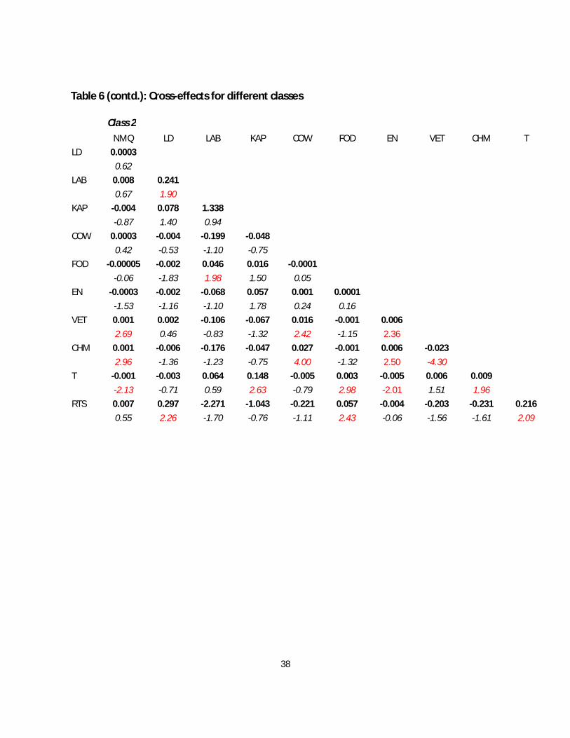
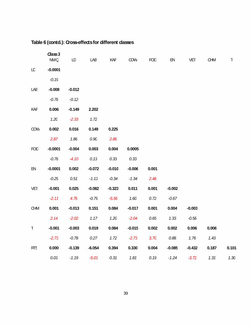
When these elasticities are presented for the different classes, in Table 6, it is clear that

different technical change bias patterns are occurring for the different technologies. In particular, for

Class 1 the marginal contribution of labor is larger and of capital is smaller and less significant –

apparently due to a larger marginal product of labor with its lower levels and a marginal product of

capital that has fallen somewhat with higher capital levels. Returns to scale are also increasing even

faster than on average, even though these farms tend to be the largest farms. By contrast, both the

marginal contributions of labor and capital are smaller for both other classes.

(table 6)

Another question about technical change is the extent to which (and which) farms switch

between classes (move to different production systems) or exit the industry. Our “preferred” estimates

with random effects for each farm and based on a panel data specification, however, group the

observations into class by farm rather than by observation, precluding consideration of such changes.

To address this question we thus must categorize the observations rather than the farms into classes.

This model is not nested and thus not directly comparable to the random effects farm-based

specification, and in fact would be expected to yield biased estimates without the panel-related random

effects. Estimating the model allows us, however, to consider whether the results are comparable and

assess farm switching and exit patterns.

26

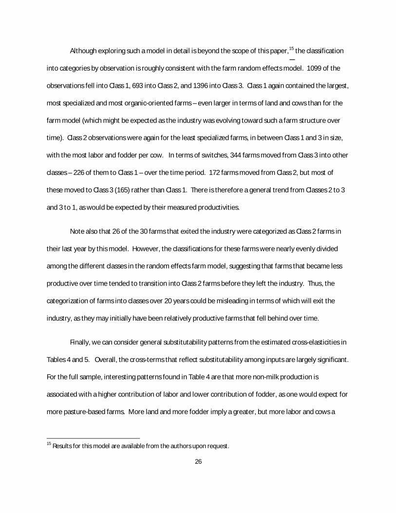
Although exploring such a model in detail is beyond the scope of this paper,15 the classification

into categories by observation is roughly consistent with the farm random effects model. 1099 of the

observations fell into Class 1, 693 into Class 2, and 1396 into Class 3. Class 1 again contained the largest,

most specialized and most organic-oriented farms – even larger in terms of land and cows than for the

farm model (which might be expected as the industry was evolving toward such a farm structure over

time). Class 2 observations were again for the least specialized farms, in between Class 1 and 3 in size,

with the most labor and fodder per cow. In terms of switches, 344 farms moved from Class 3 into other

classes – 226 of them to Class 1 – over the time period. 172 farms moved from Class 2, but most of

these moved to Class 3 (165) rather than Class 1. There is therefore a general trend from Classes 2 to 3

and 3 to 1, as would be expected by their measured productivities.

Note also that 26 of the 30 farms that exited the industry were categorized as Class 2 farms in

their last year by this model. However, the classifications for these farms were nearly evenly divided

among the different classes in the random effects farm model, suggesting that farms that became less

productive over time tended to transition into Class 2 farms before they left the industry. Thus, the

categorization of farms into classes over 20 years could be misleading in terms of which will exit the

industry, as they may initially have been relatively productive farms that fell behind over time.

Finally, we can consider general substitutability patterns from the estimated cross-elasticities in

Tables 4 and 5. Overall, the cross-terms that reflect substitutability among inputs are largely significant.

For the full sample, interesting patterns found in Table 4 are that more non-milk production is

associated with a higher contribution of labor and lower contribution of fodder, as one would expect for

more pasture-based farms. More land and more fodder imply a greater, but more labor and cows a

15 Results for this model are available from the authors upon request.

27

lower, contribution of chemicals – perhaps as the marginal product of chemicals is larger for larger

farms. Further, more capital is associated with greater contributions of both cows and fodder,

consistent with trends toward larger farms with more intensive production.

When the sample is broken down into classes these patterns are quite different. For example,

more non-milk production is not associated with labor contribution for any class, and only implies a

lower fodder contribution for Class 1. It is, however, associated with a greater marginal contribution of

cows for Class 3, and of chemicals for both Class 2 and Class 3. More cows are also associated with a

greater contribution of chemicals for Class 2 but both more cows and more land imply a lower

contribution of chemicals for Class 3, while there is very little association of any other netput with

chemicals use for Class 1. Distinguishing the technologies thus appears important for representing

substitutability, but seems to imply different substitutability rather than lower overall substitutability.

Conclusions

In this study we use a latent class modelling approach to distinguish different technologies for a

representative sample of E.U. dairy producers, as an industry exhibiting significant structural changes

and differences in production systems in the past decades. The production technologies and

productivity patterns are then modelled and evaluated for the different kinds of farms using a flexible

form of a transformation function and measures of first- and second-order elasticities.

We find that overall (average) measures of technical change and biases do not well reflect

individual firms’ experiences if the technology of an industry is heterogeneous, potentially leading to

misleading policy implications. For our application, measures of various farm characteristics reflecting

intensive vs. extensive production, input intensity, organic production and specialization were used to

divide our sample of Danish farms into three classes with different technological characteristics. A fully

28

flexible form of the transformation function is supported for our data but the overall characteristics of

production in terms of netput composition seem appropriately represented by the constrained model

used to distinguish the technologies. Farms in class 1 tend to be the largest and most productive farms

with more capital intensity relative to labor. They also enjoy economies of scale that are increasing over

time, which is not evident for the smaller more traditional class 3 farms, and have the greatest rate of

technical progress. Technical change biases show a trend toward increased specialization, and

increasing marginal contributions of land, labor and fodder (which have been falling in input intensity

relative to capital and cows). Switches over time in farm types also tended to be toward the more

productive farm “model” of class 1, while substitution within technologies appears different across

technologies but somewhat limited.

These results show that overall (average) measures do not well reflect individual firms’

production patterns if the technology of an industry is heterogeneous. That is, if there is more than one

type of production frontier embodied in the data, firms with different technologies can be expected to

have different technical change patterns, both in terms of overall magnitudes and associated relative

output and input mix changes. Assuming a uniform homogenous technology, as is typical for policy

implementation and evaluation, would result in inefficient policy recommendations leading to

suboptimal industry outcomes.

In particular, the reforms of the EU dairy sector, in line with the CAP (Common Agricultural

Policy) reform in general and in anticipation of the final CAP Health Check decisions, has aimed at a

greater market orientation of production. Direct revenue support is now fully decoupled and subject to

public and animal health and environmental standards. The current quota system will be adapted over

time by increasing quotas by 1% each year from 2009 until 2013. Support for "dairy restructuring" was

acknowledged as a priority theme under the second pillar of the CAP, which targets funds to support

29

dairy farmers in preparing for the end of quotas. These measures are meant to support increased

competitiveness and help milk producers prepare for future challenges on the international scene, while

providing limited income support by way of direct payments (see Commission 2009).

However, implementation and evaluation of these policy measures treat farm’s technology as a

homogenous black box, which our results show will result in suboptimal industry guidance. That is, our

results suggest that European dairy firms at different restructuring levels exhibit different output and

input intensities, operate with different technologies and show different technical change patterns.

Policy measures aiming to foster, change or slow down such industry restructuring have to take these

technological heterogenities into account when designing effective and efficient incentive mechanisms

to trigger desired production decisions at the firm level. This seems to be especially relevant for

environmentally motivated policy measures to support less intensive production systems.

30

References

Abdulai, A. and H. Tietje. 2007. “Estimating Technical Efficiency under Unobserved Heterogeneity with Stochastic Frontier Models: Application to Northern German Dairy Farms.” European Review of Agricultural Economics 34: 393-416.

Alvarez, A., J. del Corral, D. Solis, and J.A. Perez, “Does Intensification Improve the Economic Efficiency of Dairy Farms?” Journal of Dairy Science 91:3693-3698.

Alvarez, A. and J. del Corral. 2009. “Identifying Different Technologies Within a Sample Using a Latent Class Model: Extensive Versus Intensive Dairy Farms.” Forthcoming, European Review of Agricultural Economics.

Alvarez, A., J. del Corral, and L.W. Tauer. 2009. “Detecting Technological Heterogeneity in New York Dairy Farms.” Cornell University Working Paper.

Antonelli C. 1995. The Economics of Localized Technological Change and Industrial Dynamics. Dordrecht:Kluwer.

Atkinson, B.A. and J. Stiglitz. 1969. “A New View of Technological Change. “ The Economic Journal 79:573-578.

Battese, G., P. Rao, and C. O’Donnell. 2004. “A Metafrontier Production Function for Estimation of Technical Efficiencies and Technology Gaps for Firms Operating under Different Technologies.” Journal of Productivity Analysis 21: 91-103.

Cameron, C. and P.K. Trivedi. 2005. Microeconometrics: Methods and Applications. Cambridge University Press, New York.

Caves, D.W., L.R. Christensen and W.E. Diewert. 1982. "The Economic Theory of Index Numbers and the Measurement of Input, Output and Productivity.” Econometrica 50:1393-1414.

Commission of the European Communities. 2009. Communication from the Commission to the Council – Dairy Market Situation 2009. Brussels 27/7/2009.

Diewert, W.E., 1973. “Functional Forms for Profit and Transformation Functions.” Journal of Economic Theory 6:284-316.

Felthoven, R.G., M. Torres and C.J.M Paul. 2009. “Measuring Productivity Change and its Components for Fisheries: The Case of the Alaskan Pollock Fishery, 1994-2003” Natural Resource Modeling 22(1):105-136.

Gallant, A.R. and A. Holly. 1980. “Statistical Inference in an Implicit, Nonlinear, Simultaneous Equation Model in the Context of Maximum Likelihood Estimation.” Econometrica 48:697–720.

31

Gillespie, J., R. Nehring, C. Hallahan, C. J. Morrison Paul and C. Sandretto, 2009. “Economics and Productivity of Organic versus Non-organic Dairy Farms in the United States.” Manuscript, ERS/USDA.

Greene, W. 2002. “Alternative Panel Data Estimators for Stochastic Frontier Models.” Working Paper, Department of Economics, Stern School of Business, NYU.

Greene, W. 2005. “Reconsidering Heterogeneity in Panel Data Estimators of the Stochastic Frontier Model.” Journal of Econometrics 126(2):269-303.

Griliches, Z. 1957. “Specification Bias in Estimates of Production Functions.” Journal of Farm Economics 49:8-20.

Hoch, I. 1962. “Estimation of Production Function Parameters Combining Time-Series and Cross-Section Data.” Econometrica 30: 34-53.

Huang, H. 2004. “Estimation of Technical Inefficiencies with Heterogeneous Technologies.” Journal of Productivity Analysis 21: 277-296.

Kalirajan, K.P. and M.B. Obwona. 1994. “Frontier Production Function: The Stochastic Coefficients Approach.” Oxford Bulletin of Economics and Statistics 56: 87-96.

Kumbhakar, S., E. Tsionas and T. Sipiläinen. 2009. “Joint Estimation of Technology Choice and Technical Efficiency: an Application to Organic and Conventional Dairy Farming.” Forthcoming, Journal of Productivity Analysis.

Maudos, J., J. Pastor, and F. Pérez. 2002. “Competition and Efficiency in the Spanish Banking Sector: the Importance of Specialization.: Applied Financial Economics 12: 505-516.

Newman, C. and A. Matthews. 2006. “The Productivity Performance of Irish Dairy Farms 1984-2000: a Multiple Output Distance Function Approach.” Journal of Productivity Analysis 26: 191-205.

Nicholson, W., and C. Snyder. 2008. “Microeconomic Theory.” 10th ed., Thomson South-Western Publishers, Ohio.

Oehlert, G.W. 1992. “A Note on the Delta Method.” American Statistician 46:27-29.

Orea, L. and S.C. Kumbhakar. 2004. “Efficiency Measurement Using a Latent Class Stochastic Frontier Model.” Empirical Economics. 29:169-183

Paul, C.J.M. and R. Nehring. 2005. “Product Diversification, Production Systems, and Economic Performance in U.S. Agricultural Production.” Journal of Econometrics 126:525-548

Perrot, C., C., Coulomb, G., You and V. Chatellier. 2007. Labour Productivity and Income in North-European Dairy Farms - Diverging Models. INRA Nr. 364.

Tauer, L.W., and K. Belbase. 1987. “Technical Efficiency of New York Dairy Farms.” Northeastern Journal of Agricultural and Resource Economics 16:10-16.

32

Tauer, L.W., 1998. “Cost of Production for Stanchion versus Parlor Milking in New York.” Journal of Dairy Science 81:567-569.

(table A1)

(table A2)

33

Table 1: First-order and own second-order production structure elasticities

Full sample, constrained and full generalized linear model

(standard errors from the delta method)

FIRST ORDER No cross terms Full cross-terms

elasticity estimate t-stat elasticity estimate t-stat

M,NMQ -0.168 -15.34 M,NMQ -0.128 -10.61

M,LD 0.121 9.34 M,LD 0.104 7.20

M,LAB 0.056 3.10 M,LAB 0.039 2.11

M,KAP 0.156 10.58 M,KAP 0.159 10.61

M,COW 0.504 28.79 M,COW 0.495 26.28

M,FOD 0.212 18.51 M,FOD 0.233 18.75

M,EN 0.023 3.70 M,EN 0.032 4.19

M,VET 0.129 19.74 M,VET 0.110 16.19

M,CHM 0.017 3.02 M,CHM 0.023 3.24

M,T 0.013 4.70 M,T 0.025 4.30

Y,X 1.043 106.80 Y,X 1.060 93.43

OWN SECOND ORDER elasticity estimate t-stat elasticity estimate t-stat

NMQ,NMQ -0.0002 -8.89 NMQ,NMQ -0.0002 -4.60

LD,LD -0.003 -1.08 LD,LD -0.013 -3.02

LAB,LAB -0.157 -0.08 LAB,LAB -1.470 -0.43

KAP,KAP -1.025 -3.25 KAP,KAP -3.046 -4.95

COW,COW -0.040 -8.05 COW,COW -0.020 -3.07

FOD,FOD -0.0003 -3.26 FOD,FOD -0.001 -4.56

EN,EN -0.007 -5.20 EN,EN -0.003 -2.14

VET,VET -0.014 -3.16 VET,VET -0.029 -3.08

CHM,CHM -0.011 -1.71 CHM,CHM -0.006 -0.80

T,T -0.045 -4.16 T,T -0.068 -6.65

34

Table 2: q-variable coefficients for technology classes

Three classes Class 1 estimate t-stat

0 4.851 2.60

FOD/COW 0.049 0.66

ORG/TOT 2.434 3.16

LAB/COW -32.173 -3.79

MLK/TOT -13.445 -2.12

Class 2

0 15.369 5.38

FOD/COW -0.176 -1.82

ORG/TOT -0.027 -0.01

LAB/COW -51.947 -3.94

MLK/TOT -51.116 -5.52

Class 3 0 0

FOD/COW 0

ORG/TOT 0

LAB/COW 0

MLK/TOT 0

prior class probabilities

Class 1 Class 2 Class 3

0.388 0.077 0.535

posterior probabilities

(average for each class grouping) 0.987 0.974 0.978

35

Table 4: 1st order and own 2nd order elasticities for different classes

Full generalized linear model

FIRST ORDER Class 1 Class 2 Class 3

elasticity estimate t-stat elasticity estimate t-stat elasticity estimate t-stat

M,NMQ -0.184 -10.19 M,NMQ -0.080 -4.68 M,NMQ -0.058 -5.33

M,LD 0.138 6.32 M,LD 0.032 1.46 M,LD 0.029 2.47

M,LAB 0.109 3.96 M,LAB 0.245 8.85 M,LAB 0.089 5.80

M,KAP 0.124 5.40 M,KAP 0.196 9.16 M,KAP 0.208 15.64

M,COW 0.523 18.57 M,COW 0.451 16.79 M,COW 0.463 25.81

M,FOD 0.203 11.39 M,FOD 0.144 8.16 M,FOD 0.201 17.09

M,EN 0.023 2.43 M,EN 0.055 4.06 M,EN 0.012 1.64

M,VET 0.087 8.61 M,VET 0.041 4.15 M,VET 0.057 9.40

M,CHM 0.029 3.23 M,CHM 0.001 0.06 M,CHM 0.006 1.16

M,T 0.029 3.07 M,T 0.013 1.90 M,T 0.016 2.63

Y,X 1.043 65.63 Y,X 1.079 63.04 Y,X 1.008 97.27

OWN SECOND ORDER elasticity estimate t-stat elasticity estimate t-stat elasticity estimate t-stat

NMQ,NMQ -0.0004 -0.98 NMQ,NMQ -0.0002 -2.88 NMQ,NMQ -0.0001 -0.91

LD,LD -0.002 -0.41 LD,LD -0.011 -1.69 LD,LD -0.004 -0.65

LAB,LAB -11.239 -2.01 LAB,LAB -3.329 -0.75 LAB,LAB -8.442 -2.62

KAP,KAP -1.465 -1.83 KAP,KAP -2.376 -3.18 KAP,KAP -1.640 -1.61

COW,COW -0.017 -2.24 COW,COW -0.014 -0.99 COW,COW -0.049 -3.31

FOD,FOD -0.0002 -1.35 FOD,FOD -0.001 -4.44 FOD,FOD -0.001 -3.28

EN,EN -0.004 -2.64 EN,EN -0.004 -2.65 EN,EN -0.002 -1.15

VET,VET -0.034 -2.77 VET,VET -0.031 -2.24 VET,VET -0.059 -4.87

CHM,CHM -0.002 -0.24 CHM,CHM -0.010 -1.41 CHM,CHM -0.020 -2.03

T,T -0.068 -3.01 T,T -0.050 -4.70 T,T -0.062 -8.68

36

Table 5: Cross-elasticities for full generalized linear model Full Sample

NMQ LD LAB KAP COW FOD EN VET CHM T

LD -0.00001

-0.04

LAB 0.046 0.067

5.10 0.75

KAP 0.003 -0.030 -0.530

0.86 -0.84 -0.51

COW -0.0005 0.008 -0.074 0.183

-1.08 1.64 -0.54 3.43

FOD -0.0002 0.0004 0.017 0.022 -0.001

-3.20 0.74 1.01 3.35 -0.68

EN -0.0003 -0.005 -0.003 -0.009 0.009 0.0002

-1.73 -2.69 -0.06 -0.41 3.64 0.72

VET 0.002 -0.003 -0.486 -0.008 0.027 0.0001 0.0002

5.54 -0.78 -5.17 -0.20 5.58 0.23 0.12

CHM -0.0003 0.019 -0.535 -0.029 -0.010 0.002 0.004 -0.00008

-0.64 4.73 -4.83 -0.56 -1.90 2.98 2.17 -0.02

T -0.002 0.018 0.177 0.209 -0.030 0.002 -0.005 0.004 -0.003

-5.27 4.82 1.92 4.39 -5.92 2.93 -2.69 0.98 -0.61

RTS 0.049 0.044 -3.161 -3.457 0.121 0.041 -0.005 -0.499 -0.555 0.371

5.43 0.50 -3.03 -3.41 0.85 2.43 -0.11 -5.34 -4.85 4.19

37

Table 6: Cross-effects for different classes Class 1


LD 0.0004

1.18

LAB 0.023 -0.071

1.82 -0.60

KAP 0.003 0.013 -2.229

0.83 0.31 -1.57

COW -0.0005 -0.011 -0.007 0.202

-0.81 -1.79 -0.04 2.79

FOD -0.0002 0.002 0.015 -0.002 -0.002

-2.66 3.29 0.64 -0.22 -2.38

EN -0.001 0.003 -0.122 0.004 0.002 0.0004

-2.48 1.34 -1.77 0.14 0.74 0.87

VET 0.002 -0.016 -0.513 -0.057 0.037 -0.001 -0.006

5.62 -4.03 -4.20 -1.13 5.75 -0.80 -2.18

CHM -0.001 0.004 -0.056 -0.019 -0.004 0.001 0.001 0.016

-1.69 0.70 -0.34 -0.25 -0.57 1.29 0.53 2.51

T -0.003 0.017 0.611 0.109 -0.027 0.002 -0.005 0.011 0.010

-5.66 2.84 3.42 1.33 -3.29 1.91 -1.56 1.82 1.26

RTS 0.026 -0.078 -14.549 -3.563 0.200 0.013 -0.120 -0.574 -0.059 0.726

2.10 -0.66 -9.99 -2.55 1.00 0.59 -1.69 -4.83 -0.36 4.43

38

Table 6 (contd.): Cross-effects for different classes Class 2


LD 0.0003

0.62

LAB 0.008 0.241

0.67 1.90

KAP -0.004 0.078 1.338

-0.87 1.40 0.94

COW 0.0003 -0.004 -0.199 -0.048

0.42 -0.53 -1.10 -0.75

FOD -0.00005 -0.002 0.046 0.016 -0.0001

-0.06 -1.83 1.98 1.50 0.05

EN -0.0003 -0.002 -0.068 0.057 0.001 0.0001

-1.53 -1.16 -1.10 1.78 0.24 0.16

VET 0.001 0.002 -0.106 -0.067 0.016 -0.001 0.006

2.69 0.46 -0.83 -1.32 2.42 -1.15 2.36

CHM 0.001 -0.006 -0.176 -0.047 0.027 -0.001 0.006 -0.023

2.96 -1.36 -1.23 -0.75 4.00 -1.32 2.50 -4.30

T -0.001 -0.003 0.064 0.148 -0.005 0.003 -0.005 0.006 0.009

-2.13 -0.71 0.59 2.63 -0.79 2.98 -2.01 1.51 1.96

RTS 0.007 0.297 -2.271 -1.043 -0.221 0.057 -0.004 -0.203 -0.231 0.216

0.55 2.26 -1.70 -0.76 -1.11 2.43 -0.06 -1.56 -1.61 2.09

39

Table 6 (contd.): Cross-effects for different classes Class 3


LD -0.0001

-0.19

LAB -0.008 -0.012

-0.78 -0.12

KAP 0.006 -0.149 2.202

1.20 -2.33 1.72

COW 0.002 0.016 0.149 0.225

2.87 1.86 0.90 2.86

FOD -0.0001 -0.004 0.003 0.004 0.0005

-0.78 -4.10 0.13 0.33 0.33

EN -0.0001 0.002 -0.072 -0.010 -0.006 0.001

-0.29 0.51 -1.13 -0.34 -1.34 2.48

VET -0.001 0.025 -0.082 -0.323 0.011 0.001 -0.002

-2.11 4.78 -0.79 -5.56 1.60 0.72 -0.67

CHM 0.001 -0.013 0.151 0.084 -0.017 0.001 0.004 -0.003

2.14 -2.02 1.17 1.20 -2.04 0.65 1.33 -0.58

T -0.001 -0.003 0.019 0.084 -0.015 0.002 0.002 0.006 0.006

-2.73 -0.78 0.27 1.72 -2.73 3.70 0.88 1.76 1.43

RTS 0.000 -0.139 -6.054 0.394 0.330 0.004 -0.085 -0.432 0.187 0.101

0.03 -1.19 -5.03 0.31 1.81 0.19 -1.24 -3.72 1.31 1.30

40

Table A1: Summary Statistics of the data (whole sample, classes, and over time)

Full Sample Mean Std. Dev. Minimum Maximum No. observations

Milk (1000 kg) 453.91 263.35 2.50 1624.37 3188 Milk 1204.06 647.73 7.01 3785.38 Non-Milk Output 624.09 445.50 0.00 5298.58 Total output 1828.15 925.92 51.51 6590.93 Land (hectares) 76.80 44.33 14.30 270.00 Labor (000 hours/year) 4.27 1.49 1.20 11.80 Capital (million Kronor) 6.23 4.60 0.76 33.00 Cows (number) 68.21 33.59 2.00 223.00 Fodder (purchased) 357.51 228.38 8.00 2165.06 Energy (Mwh) 62.60 49.29 0.21 369.40 Veterinary 40.88 29.14 0.00 286.64 Chemicals 26.27 22.73 0.00 154.73

Milk/total (revenue) 0.661 0.126 0.004 1.000 Organic/total (revenue) 0.069 0.218 0.000 1.000 Fodder/Cow 5.311 2.525 0.364 36.084 Labor/Cow 0.071 0.071 0.027 3.800

Note: All variables for which units are not specified are in thousands of Danish Kroner deflated to the base year 1986 using a producer price index (for agricultural materials, milk and dairy products, or machinery and buildings, as appropriate) Source: Landscentret Denmark and Danmark Statistic

41

Table A1 (contd): Summary Statistics of the data (classes)

Class 1

Mean Std. Dev. Minimum Maximum No. observations Milk (kg) 676.69 285.31 6.91 1624.37 1054 Milk 1728.28 674.03 16.13 3785.38 Non-Milk Output 855.56 520.84 0.00 5298.58 Total output 2583.84 896.63 606.41 6590.93 Land (hectares) 108.58 42.67 23.60 270.00 Labor (hours/year) 5.19 1.45 2.11 11.80 Capital 9.16 5.16 1.90 28.48 Cows (number) 92.81 34.38 2.00 221.00 Fodder (purchased) 495.08 263.94 51.02 2165.06 Energy (Mwh) 78.78 63.69 0.21 369.40 Veterinary 57.86 35.10 0.00 286.64 Chemicals 33.01 28.23 0.00 153.34


42


Class 2 Mean Std. Dev. Minimum Maximum No. observations

Milk (kg) 354.47 167.97 7.48 1144.15 810 Milk 1053.95 516.28 11.80 3213.86 Non-Milk Output 606.31 400.01 0.00 2759.72 Total output 1660.26 750.72 213.34 5080.33 Land (hectares) 71.36 42.33 14.50 238.50 Labor (hours/year) 4.27 1.49 1.60 10.10 Capital 5.75 4.17 1.06 33.00 Cows (number) 64.87 28.14 20.00 177.00 Fodder (purchased) 322.62 154.59 33.90 1309.90 Energy (Mwh) 65.13 44.91 0.41 286.11 Veterinary 35.04 21.65 0.00 172.12 Chemicals 28.35 23.52 0.00 154.73


43


Class 3 Mean Std. Dev. Minimum Maximum No. observations



44

Table A1 (contd): Summary Statistics of the data (over time)

1986 Mean Std. Dev. Minimum Maximum No. observations



2005

Mean Std. Dev. Minimum Maximum No. observations Milk (kg) 825.933 329.882 134.332 1437.830 84 Milk 1915.090 766.010 253.643 3475.080 Non-Milk Output 275.649 223.870 0.000 1214.960 Total output 2190.740 863.214 319.824 3800.040 Land (hectares) 113.169 51.582 14.500 243.700 Labor (hours/year) 4.806 1.356 2.404 9.100 Capital 13.902 5.832 3.705 26.854 Cows (number) 105.607 34.755 31.000 189.000 Fodder (purchased) 498.717 242.046 93.021 1827.950 Energy (Mwh) 63.886 84.033 0.415 369.400 Veterinary 56.701 31.275 5.057 148.190 Chemicals 15.445 21.616 0.000 74.143


45

Table A2: Transformation function estimates Full sample, constrained and full generalized linear model

No cross-terms Full cross-terms coefficient estimate t-stat coefficient estimate t-stat

a0 -69.430 -1.89 a0 -17.680 -0.41 aLDEN -1.276 -2.69

a0NMQ 6.764 6.52 a0NMQ 0.157 0.06 aLDVET -0.584 -0.78

a0LD 9.891 1.81 a0LD -16.857 -1.91 aLDCHM 3.416 4.73

a0LAB 4.560 0.10 a0LAB 25.762 0.41 aLABKAP -10.939 -0.51

a0KAP -23.565 -1.65 a0KAP -34.823 -1.20 aLABCOW -5.056 -0.54

a0COW -41.561 -5.40 a0COW -0.392 -0.03 aLABFOD 2.667 1.01

a0FOD 9.088 4.99 a0FOD 0.289 0.08 aLABEN -0.168 -0.06

a0EN -8.799 -4.80 a0EN -6.232 -1.43 aLABVET -25.674 -5.17

a0VET 15.674 5.01 a0VET 13.261 2.25 aLABCHM -22.684 -4.83

a0CHM -3.042 -1.29 a0CHM 20.401 3.37 aKAPCOW 15.074 3.43

bT 5.031 4.31 bT 3.291 1.13 aKAPFOD 4.224 3.35

bTT -0.197 -3.06 bTT -0.507 -5.17 aKAPEN -0.746 -0.41

aNMQNMQ -0.257 -13.63 aNMQNMQ -0.307 -6.71 aKAPVET -0.492 -0.20

aLDLD 0.154 0.54 aLDLD -1.327 -2.10 aKAPCHM -1.492 -0.56

aLABLAB 4.884 0.44 aLABLAB -8.398 -0.29 aCOWFOD -0.360 -0.68

aKAPKAP 16.077 7.23 aKAPKAP -26.330 -3.54 aCOWEN 2.336 3.64

aCOWCOW 5.870 13.58 aCOWCOW 0.560 0.63 aCOWVET 5.615 5.58

aFODFOD 0.029 0.68 aFODFOD -0.189 -1.80 aCOWCHM -1.758 -1.90

aENEN 0.722 5.72 aENEN 0.557 3.25 aFODen 0.150 0.72

aVETVET 0.204 0.89 aVETVET -1.332 -3.84 aFODVET 0.063 0.23

aCHMCHM 0.587 2.44 aCHMCHM 0.083 0.22 aFODCHM 0.923 2.98 aNMQLD -0.009 -0.04 aENVET 0.046 0.12

aNMQLAB 9.543 5.10 aENCHM 0.710 2.17

aNMQKAP 0.688 0.86 aVETCHM -0.010 -0.02

aNMQCOW -0.411 -1.08 bNMQT -0.568 -5.27

aNMQFOD -0.334 -3.20 bLDT 1.933 4.82

aNMQEN -0.254 -1.73 bLABT 4.614 1.92

aNMQCHM 1.127 5.54 bKAPT 6.565 4.39

aNMQVET -0.138 -0.64 bCOWT -3.104 -5.92

aLDLAB 4.838 0.75 bFODT 0.461 2.93

aLDKAP -2.638 -0.84 bENT -0.523 -2.69

aLDCOW 2.373 1.64 bVETT 0.284 0.98

aLDFOD 0.278 0.74 bCHMT -0.164 -0.61

Distinguishing Different Industry Technologies and - AgEcon Search

Documents

Transcript of Distinguishing Different Industry Technologies and - AgEcon Search