Display Advertising Pricing in Exchange Markets

Hana Choi∗ Carl F. Mela†

November 10, 2019

Abstract

This paper considers how a publisher should set reserve prices for real-time bidding

(RTB) auctions when selling display advertising impressions through ad exchanges, a

$50 billion market and growing. Through a series of field experiments, we find that

setting the reserve price increases publisher’s revenues by 32%, thereby affirming the

importance of reserve price in maximizing publisher’s revenues from auctions. Further,

we find that advertisers increase their bids in response to an experimental increase in

reserve price and show this behavior is consistent with the use of a minimum impression

constraint to ensure advertising reach.

Based on this insight, we construct an advertiser bidding model and use it to infer

the overall demand curve for advertising as a function of reserve prices. Using this

demand model, we solve the publisher pricing problem. Incorporating the minimum

impression constraint into the reserve price setting process yields a 50% increase over a

solution that does not incorporate the constraint and an additional increase in profits

of nine percentage points.

∗Assistant Professor of Marketing at the Simon School of Business, Univeristy of Rochester (email:hana.choi@rochester.edu, phone: 585-275-0790)†The T. Austin Finch Foundation Professor of Business Administration at the Fuqua School of Business,

Duke University (email: mela@duke.edu, phone: 919-660-7767).The authors thank Santiago Balseiro, Bryan Bollinger, Giuseppe Lopomo, Hema Yoganarasimhan, and

seminar participants at Boston University, City University of Hong Kong, the University College London,Cornell University, Duke-UNC Brownbag, the University of Georgia, Harvard University, HEC Paris, HKUST,the University of Illinois at Urbana-Champaign, Johns Hopkins University, Lingnan University, the Universityof Miami, Northwestern University, the University of Notre Dame, Rice University, the University of Rochester,Southern Methodist University, Stanford University, the University of Texas at Austin, Tilburg University,and Yonsei University for comments and suggestions.

1 Introduction

1.1 Overview

Display advertising (display ad herein) markets exist to match advertisers to publishers. This

paper considers how a publisher should set reserve prices for auctions when selling display

advertising impressions in real-time through ad exchanges, a topic of growing economic

importance. Display ad markets are estimated to be $49.8 billion in the US in 2018, growing

considerably from $39.4 billion in 2017.1 Drivers behind this 26% double-digit growth

rate include an upswing in mobile activities, a proliferation in online video ad formats, and

technological advancements in real-time buying (RTB) through ad exchange auctions. Display

ad spending have surpassed even search ad spending and is forecasted to continue its rapid

revenue ascent.2 In spite of this, empirical research into publisher’s strategies and advertiser

behaviors in display markets is limited. This paper seeks to begin filling this void.

Publishers in display ad markets (e.g., CNN, Wall Street Journal, Facebook, Youtube) are

selling a growing number of their advertising impressions on their sites through ad exchanges.3,4

Ad exchanges (e.g., DoubleClick Ad Exchange, OpenX, Rubicon) are centralized marketplaces

where publishers supply and advertisers demand display advertising impressions in real time,

as consumers browse the pages upon the publishers’ sites. To achieve this aim, the publisher

first makes the impression available to the ad exchange. Second, the ad exchange then runs

an auction for this incoming impression and requests bids from the advertisers. Ad exchanges

typically conduct a second-price, sealed-bid auction for each impression instantaneously as it

becomes available, thus selling and buying through ad exchanges is often called real-time

buying or real-time bidding (RTB). Finally, the winner’s ad is served to the consumer. The

1 https://www.iab.com/wp-content/uploads/2019/05/Full-Year-2018-IAB-Internet-Advertising-Revenue-Report.pdf2 Search advertising revenue totaled $48.4 billion in 2018, a little below display advertising, and the growthrate is abating (19.2%).3 https://www.emarketer.com/content/more-than-80-of-digital-display-ads-will-be-bought-programmatically-in-20184 In 2018, RTB accounts for 35% of the total display ad market in the US, and its share of the display marketis quickly increasing.

1

entire process of selling, buying, and ad serving is typically done within milliseconds.5, 6

One reason RTB is an ascendant approach to selling display advertising is that it offers

advertisers a litany of information regarding demographics, interests, and past behaviors

of the person seeing the impression on the publisher’s page, thereby affording advertisers

considerable latitude when targeting customers. The broad array of impression-level user

characteristics often integrate information from publishers (e.g., the type of articles read),

advertisers (such as past purchase), and intermediaries who collect cookie-level information.7

Moreover, because each impression is sold individually and in real time, the advertiser has

substantial flexibility over both how many exposures to buy (reach) and when and how much

to spend (budget). Both the advertisers’ valuations for impressions and constraints such as

reach or budget can influence the publisher’s pricing decisions.

Accordingly, we first consider how advertisers value ad impressions, and how advertisers’

bidding behaviors can be affected by (i) own valuations, (ii) competing valuations, and (iii)

the reach or budget constraint they face. Subsequently, we examine how the publisher should

price (set their reserve prices) in response to advertisers’ demand and bidding behaviors. To

address these two questions, we collect a novel dataset on advertiser bidding behaviors from

an ad exchange, and run a series of reserve pricing experiments in conjunction with a major

publisher. Using this exogenous variation in reserve pricing, we develop a structural model of

advertiser bidding behavior in competitive markets, and derive the optimal pricing policy on

part of the publisher selling its inventory into the exchange market.

Using a naive assumption of no constraints to set reserve prices in our experiments increases

publisher revenues an average of 32% across 12 studies, and the exogenous experimental

variation enables us to subsequently test this naive assumption of no advertiser budget

5 http://data.iab.com/ecosystem.html6 Please see Choi et al. 2017 for operational details of display ad markets.7 User characteristics together with ad unit characteristics (e.g., time of ad delivery, site where ad is placed,ad location on a page etc.) define an ad impression - the unit of sale in display ad markets. Of note, thedisplay ad auction format (typically second-price, sealed-bid auction) is different from the sponsored searchauction format (generalized second price or position auction). If a site visitor sees two ads on the site,for example one located above-the-fold and the other located below-the-fold, two independent auctions areconducted for these two ad impressions.

2

or impression constraints. Initial findings reveal that bids vary with reserves in a manner

consistent with advertisers’ use of minimum impression constraints. In the absence of a

reserve, 19% of advertisers appear to face this constraint leading them to increase their bids

by about 20%. However, as the reserve prices increase, the percentage of advertisers subject

to a binding constraint increases to 32% and their bid premium rises to 25%. The use of a

naive assumption of no constraints to set reserve prices leads to solutions 27% lower than

what the optimal reserves should be in the face of these impression constraints. We project

that our model, which accommodates these constraints, would further improve publisher

profits by about 9 percentage points.

1.2 Relevant Research

Much of the display advertising literature focuses on measuring advertising effectiveness and

the attendant consequences for advertisers’ ad buying and targeting decisions (e.g., Barajas

et al. 2016, Hoban and Bucklin 2015, Johnson, Lewis, and Nubbemeyer 2016, Johnson, Lewis,

and Reiley 2016, Lewis and Rao 2015, Sahni 2015, Sahni˙Nair˙2016, Tucker 2014, Goldfarb

and Tucker 2011, Rafieian and Yoganarasimhan 2016). In contrast, our focus is on publishers’

pricing strategies in exchange markets by inferring advertiser valuations.

Existing papers on display markets often consider each auction (i.e., each impression) to

be a single-shot game (e.g., Johnson 2013, Celis et al. 2014, Sayedi 2018). More recently,

the fields of computer science and operations research have developed optimal bidding

algorithms for advertisers who are playing repeated auctions for many impressions across

lengthy campaigns that can be affected by a number of practical constraints. These include

bidding algorithms for advertisers who (i) face budget constraints for a given campaign in

repeated auctions (Balseiro et al. 2015; Balseiro and Gur 2019), (ii) have limited information

about their own and/or others’ true valuations (Iyer et al. 2014; Cai et al. 2017), (iii) set a

number of impressions to attain (Ghosh et al. 2009), or (iv) set pacing options so that the

budget is spent smoothly over a specified time period (Lee et al. 2013; Yuan et al. 2013; Xu

et al. 2015). We build on this literature by providing empirical evidence that advertisers’

3

bidding strategies are consistent with the use of a minimum impression constraint to ensure

advertising reach. Accordingly, we accommodate the minimum impression constraint in our

advertiser bidding model as a prerequisite in solving the publisher’s pricing problem.

In recovering advertisers’ valuations in this dynamic setting, we adopt the fluid mean-field

equilibrium (FMFE) framework developed in Balseiro et al. 2015. Of note, the solution to the

advertiser bidding game only depends on the steady-state distribution of rival bids (and not

on the current single auction-specific state or the rivals’ individual states). This equilibrium

concept provides a computationally tractable way of modeling advertiser bidding behaviors

and competition while capturing the dynamic nature of the advertiser decisions across

auctions.8 We extend this framework to accommodate a minimum impression constraint, and

suggest estimation and identification strategies to link the FMFE theory to our empirical

context.

Finally, in contrast with most of this prior research, we conduct field experiments to

provide exogenous variation to test assumptions used in our model and demonstrate the

potential of using theoretical insights to improve auction outcomes. On this dimension, our

research is related to Ostrovsky and Schwarz 2011, who conduct a large field experiment in

the context of search advertising. They find that setting appropriate reserve prices guided

by theory leads to substantial increases in seller revenues. We similarly corroborate the

importance of setting reserve prices, but in the context of display ad auctions (instead of

sponsored search auctions). Different from Ostrovsky and Schwarz 2011, we additionally

examine the causal effect of reserve prices on advertiser bidding behaviors and use a structural

model to back out advertiser primitives.

1.3 Organization

This paper is organized as follows. Section 2 first characterizes our data, demonstrating

considerable heterogeneity in advertiser bidding behaviors. Next in Section 3, we present the

8 Backus and Lewis 2016 and Hendricks and Sorensen 2015 study bidders having a unit demand with multipleopportunities to bid in second-price sealed-bid auctions, and apply the framework to eBay’s market. Theyalso similarly use the belief formation and the mean-field equilibrium concept in Krusell and Smith 1998,Weintraub et al. 2008, and Iyer et al. 2014, but for a unit demand without a (reach or budget) constraint.

4

advertiser bidding model and the publisher pricing model. Section 4 discusses the estimation

method and the identification argument in inferring advertiser valuations, and Section 5

presents the estimation results. Finally in Section 6, we compute the optimal reserve prices

and the revenue gains.

2 Data

In this section, we first describe the publisher and the data source. Second, we show

that advertiser bids differ for different types of impressions. This heterogeneity in bids is

instrumental in setting reserve prices and also suggests that advertisers consider information

about impressions in their bids. Lastly, as a prelude to a bidding model and to demonstrate

the economic value of setting reserves, we consider how reserve prices affect publisher’s

revenues and advertisers’ bidding behaviors through a series of field experiments. Of note,

using theory based reserves led to a 32% increase in profits, providing concrete evidence there

is substantial room to enhance pricing outcomes for the publisher.

2.1 The Publisher and Data Source

The data for this study are collected from a large, premium publisher, ranked within the U.S.

Top 10 by comScore.9 The publisher has over 30 brands (sites) internationally, among which

we focus on the top 20 U.S.-based sites for our analyses. We further focus our attention on

display ads and exclude video in our analyses.10 The data are collected from January 2016 to

August 2017.

The publisher’s ad exchange partner provides a report on auction outcomes (related to

this publisher’s ad impressions) at the daily level, and the data provided on the various

measures are available as daily averages. These data include advertiser ID, Demand Side

Platform (DSP herein) ID,11 day, site where ad was placed, ad type (ad size, ad location

9 https://www.comscore.com/Insights/Rankings10 We adopt this sampling criterion due to the publisher’s current selling policy. Video ads are mostly sold-outin advance via the direct sales and are rarely available for sale in the ad exchange. Also the online video adsare often sold with the TV ads as a bundle, which hinders our analyses in the absence of the data on TV ads.11 Demand Side Platforms (e.g., MediaMath, DataXu, Turn, Rocket Fuel, Adobe Advertising Cloud) helpadvertisers by facilitating the real-time bidding process. Recognizing that bid optimization is a difficult

5

on a page, device), number of bids submitted, number of impressions won, bidding amount,

payment amount, and click responses. Thus the observational unit (i.e., dimension) is at the

advertiser-DSP-day-site-ad type delivered, and the metrics provided for each observational

unit are number of bids submitted, number of impressions won, bidding amount, payment

amount, and number of clicks received. Focusing on the open auctions in the ad exchange, we

have 1, 466M observations. While number of impressions won, payment amount, and number

of click responses are available for all advertisers (we call this the “payment data”), number

of bids submitted and the bidding amount are only available for a subset of advertisers who

opt-in to reveal (share) their data with the publisher (we call this the “bidding data”).

2.2 Summary Statistics

In this section we provide summary statistics of the data to show there exists considerable

variation in advertiser bidding/payment and to explain the rationale behind using the payment

data in our estimation (as opposed to using the bidding data).

Summary statistics of advertiser buying behaviors are presented in Table 1. At the

observational unit level (i.e., advertiser-DSP-day-site-ad type delivered), advertisers on

average won 70 impressions at $1.61 CPM rate. The minimum CPM payment is close to zero,

because the publisher currently imposes no reserve price in the auctions.

During the sample period, 14, 612 advertisers participated in the auctions. Bids are

observed from the 82% of the advertisers who opted-in (default setting) to share their bidding

information. Opt-in advertisers pay a higher CPM ($1.89) than the full sample average

($1.61), but buy a much smaller number of impressions, constituting about 16% of the total

revenues.

Hence, there are selection concerns arising from using the bid CPMs for inferring advertiser

valuations in estimation. Fortunately, data are available on the CPM paid (i.e, the second

highest bid in an auction). Unlike bid CPM, this CPM paid measure is available from all

advertisers. Accordingly, we rely on the payment data in our estimation, and only use number

managerial problem for the advertisers, DSPs specialize in calculating and submitting bids based on the users’behavioral data and on targeting criteria provided by the advertiser.

6

of bids submitted and bid CPM data to present evidence of heterogeneity in the bidding

behaviors in the following sub-section 2.3.

Table 1: Summary Statistics of exchange

Per Observation Unit Mean Median Std Dev Min MaxAll #Impressions Won 69.9 2 2345 0 587307

CPM paid ($) 1.61 0.86 2.74 0.003 191.5Opt-In #Impressions Won 10.1 0 1312 0 777817

CPM paid ($) 1.89 1.00 3.05 0.002 191.5# Bids Submitted 280 5 15042 1 5.4MBid CPM 2.7 1.2 67.4 0.00003 50000

2.3 Heterogeneity in Valuations

In order to understand how to set reserve prices, it is imperative for the publisher to determine

the distribution of advertiser valuations. The results below suggest substantial heterogeneity

in bids with respect to the observed characteristics. To the extent that bids reflect advertisers’

underlying valuations, the optimal reserve prices can potentially be set based on the observed

key characteristics driving the heterogeneity for better price discrimination.

First in Figure 1, we explore the distribution of bid CPMs. The x-axis represents

zscore of bid CPMs, and the y-axis represents the percentage of number of bids.12 There

exists considerable heterogeneity with the minimum of −0.28 and the maximum value being

14721.44.

To explain the variation in the advertisers’ bid CPMs, we estimate a weighted least square

12 Bid CPM data are daily averages. Thus in calculating the zscore, we use the weighted mean and weightedstandard deviation, where the number of bids for a given observational unit is used as the weight.

Table 2: Advertiser Bid CPM: Weighted Least Square Regression

DV: Bid CPM ZScore EstimatesDesktop 0.059 (0.007)Mobile −0.062 (0.006)Tablets −0.057 (0.006)Display vs. App 0.149 (0.004)Above the Fold vs. No info 0.005 (0.004)Mid vs. No info −0.012 (0.004)Below the Fold vs. No info −0.013 (0.005)Site YesAdvertiser YesDays (control for supply, competition) Yes

7

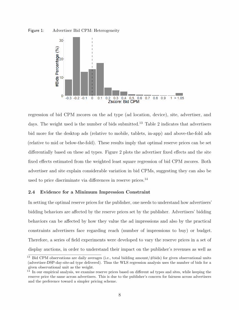
Figure 1: Advertiser Bid CPM: Heterogeneity

regression of bid CPM zscores on the ad type (ad location, device), site, advertiser, and

days. The weight used is the number of bids submitted.13 Table 2 indicates that advertisers

bid more for the desktop ads (relative to mobile, tablets, in-app) and above-the-fold ads

(relative to mid or below-the-fold). These results imply that optimal reserve prices can be set

differentially based on these ad types. Figure 2 plots the advertiser fixed effects and the site

fixed effects estimated from the weighted least square regression of bid CPM zscores. Both

advertiser and site explain considerable variation in bid CPMs, suggesting they can also be

used to price discriminate via differences in reserve prices.14

2.4 Evidence for a Minimum Impression Constraint

In setting the optimal reserve prices for the publisher, one needs to understand how advertisers’

bidding behaviors are affected by the reserve prices set by the publisher. Advertisers’ bidding

behaviors can be affected by how they value the ad impressions and also by the practical

constraints advertisers face regarding reach (number of impressions to buy) or budget.

Therefore, a series of field experiments were developed to vary the reserve prices in a set of

display auctions, in order to understand their impact on the publisher’s revenues as well as

13 Bid CPM observations are daily averages (i.e., total bidding amount/#bids) for given observational units(advertiser-DSP-day-site-ad type delivered). Thus the WLS regression analysis uses the number of bids for agiven observational unit as the weight.14 In our empirical analysis, we examine reserve prices based on different ad types and sites, while keeping thereserve price the same across advertisers. This is due to the publisher’s concern for fairness across advertisersand the preference toward a simpler pricing scheme.

8

Figure 2: Advertiser Bid CPM: Advertiser and Site Fixed Effects

9

on the advertisers’ bidding behaviors.

The theoretical prediction under the standard second-price, sealed-bid auction format is

that bidders bid truthfully, meaning that advertisers’ underlying valuations can directly be

inferred from the observed bids. Though the assumption of truth-telling strategy is tractable

and often assumed in models of display markets (e.g., Celis et al. 2014, Sayedi 2018), there

exists some empirical evidence that advertisers face practical constraints when bidding in the

exchange auctions. We begin by outlining the practical constraints advertisers might face

when bidding in the exchange. Then we provide evidence that advertisers’ bidding behaviors

are not consistent with truth-telling, but appear to reflect a minimum impression constraint.

2.4.1 Practical Constraints in Bidding

Practical constraints discussed in existing literature include (i) budget constraint (Balseiro

et al. 2015; Balseiro and Gur 2019), (ii) imperfect information about own and/or other’s true

valuations (Iyer et al. 2014; Cai et al. 2017), (iii) minimum impression goal (Ghosh et al. 2009),

and (iv) pacing options where the budget is spent smoothly over a specified time period

(Lee et al. 2013; Yuan et al. 2013; Xu et al. 2015). Advertisers’ optimal bidding strategies

may deviate from their true valuations when faced with these practical constraints. If one or

more of these constraints seem to bind advertisers’ bidding behaviors, those constraints will

need to be considered in building the advertiser bidding model. Otherwise, predictions of

advertisers’ bidding behaviors under the counterfactual (e.g., when increasing the reserve

prices) will be incorrect and will lead to wrong inference on the optimal reserve prices.

Table 3: Theory Predictions

Mechanism Reserve Level Effect of Imposing Reserver = 0 r = r∗nc > 0 Bid CPM #Impressions Won Total Payment

Max Budget Constraint Not Bind Not Bind No Change − +Not Bind Bind − − +

Bind Bind +/− +/− No ChangeMin Impression Constraint Not Bind Not Bind No Change − +

Not Bind Bind + − +/−Bind Bind + No Change +

Our goal then is to change reserve prices and see how advertisers respond in order to

10

determine which mechanism stands out as the main driver behind their behaviors. Table 3

presents the theory predictions on bid CPM, the number of impressions won, and the total

payment, when the reserve price is changed from r = 0 (i.e., no reserve) to r∗nc > 0. r∗nc is

the optimal reserve calculated under the no constraint, single-shot (truth-telling) model.15

As the reserve price increases from (r = 0) to (r∗nc > 0), advertisers face tighter constraints,

and each row represents a possible scenario of the underlying state: (not bind, not bind),

(not bind, bind), (bind, bind). Each mechanism is considered in isolation. That is, when we

consider the budget constraint, we assume that the minimum impression constraint does not

bind in both (r = 0) and (r∗nc > 0).

In sum, by varying the reserve and observing how the metrics change, we can determine

which of these explanations is most consistent with the data and ensure our advertiser bidding

model specification is consistent with the bidding outcomes.

2.4.2 Experimental Setting

Twelve field experiments were conducted on select websites and the pairs (a treatment and a

control) were chosen to be closest in terms of ad characteristics, contents, user demographics,

revenues, and number of impressions (user visits).16 The experiments spanned the period

08/01/2017 - 12/03/2017, where 08/01/2017 - 10/15/2017 constitute the ‘Prior’ period

and 10/19/2017 - 12/03/2017 constitute the ‘Post’ period in which the reserve prices were

changed for the treatment group. The experimental reserve prices in the treatment condition

were calculated using a naive theoretical model presuming that advertisers do not face

any constraints and that advertisers play a single-shot game for each available impression.17

15 Online Appendix B.2 outlines the rationale for these predictions, as well as the pacing option and imperfectinformation cases alluded to above.16 These pairs (a treatment and a control) were randomized either into the treatment or the control group.For example, (site1, desktop, BTF, 300x250) and (site1, desktop, ATF, 300x250) were paired for the firstexperiment, and the randomly chosen (site1, desktop, BTF, 300x250) was assigned to the treatment group,and (site1, desktop, ATF, 300x250) was assigned to the control group. Details of the experimental groups areincluded in Table 9 in online Appendix.17 Changes in advertiser bidding behaviors with respect to exogenous changes in reserve prices are required tovalidate theoretical predictions regarding the existence of a budget or impression constraint. However, tovalidate predictions about how bids can change with respect to constraints, the level of the treatment reserveprices need not be at the optimal level, merely that the reserves vary exogenously. As such, the suggestedexperimental reserve prices provide the first order approximations of the optimal reserve prices, and are likely

11

During the ‘Post’ period, the reserve prices were set to these calculated levels for the treatment

group, while they were kept at the historical levels for the control group (i.e., no reserve

prices). The details of the experiment design and calculating the experimental reserve prices

can be found in online Appendix A.

2.4.3 Experimental Results on eCPM

We begin by reporting experimental results regarding the publishers’ revenues to gauge the

effectiveness of setting reserve prices in auctions.

Effect on eCPM The outcome measure considered is eCPM (effective CPM, industry

vernacular), which yields a per supplied impression revenue.

eCPM =Revenue

# Impression Supplied to Exchange (in thousand)

Table 4 shows the treatment effect on eCPM, where eCPM is multiplied by a common,

multiplicative constant for confidentiality. The increase in revenues (holding the impressions

supplied to exchange the same) is huge, 32%, thereby affirming the importance of setting the

reserve prices in running auctions.

Increase in revenue =(0.49− 0.38)− (0.33− 0.34)

0.38

=0.12

0.38' 32%

Table 4: Treatment Effect on eCPM

Group Reserve Prior(08/01/17 - 10/15/17)

Post(10/19/17 - 12/03/17)

Treatment Yes 0.38 0.49Control No 0.34 0.33

Note: eCPM is scaled by multiplicative constant for confidentiality.

Figure 3 plots the treatment effect by the experimental groups, and includes a dotted

horizontal line representing the weighted average percentage change in eCPM across treatments,

to increase the publisher’s revenues close to the global maximum. Further improvements are possible whenconstrained bidding is considered, as we shall discuss later.

12

32%. Differences in treatment effects across experiments can largely be explained by the

observed characteristics of the site-ad type used in the various experiments, and the results

from a formal difference-in-difference analysis on eCPM is reported in Table 10 in online

Appendix.

Figure 3: Treatment Effect on eCPM by Group

0

50

100

150

200

1 2 3 4 5 6 7 8 9 10 11 12Experiments

Cha

nge

in e

CP

M (

%)

2.4.4 Experimental Results on Bidding Behaviors

To assess how advertisers’ bidding behaviors are affected by the (exogenous) increase in

reserve prices, we consider their bid CPM data. If advertisers bid truthfully, the distribution

of bids will remain invariant to the experimental manipulation of the reserve price. However,

this is not the case. Figure 4 plots the distribution of changes in bids for those advertisers

bidding both in the ‘Prior’ and ‘Post’ periods for a given (site-ad type). The changes are

computed as the advertiser’s average bid CPM in the ‘Post’ minus that in the ‘Prior’ period.

The probability density function’s mass is greater in the positive region, meaning advertisers

increase their bids in the ‘Post’ period in response to an increase in the reserve price.18

Turning to a difference-in-difference (DiD) analysis of the experimental outcomes for bids,

the first column in Table 5 presents the results of a DiD analysis that controls for a time

18 If the advertiser’s cost to participate in the auction is high, the advertiser might not submit bids in the‘Post’ period should the reserve price exceed its valuation. To account for this truncation in the observeddata for the treatment group, we analyze both the prior- and post- bids that are above the reserve price usedin the post period, and find a similar pattern.

13

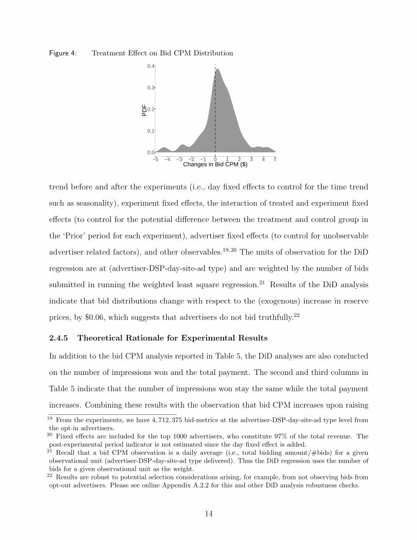
Figure 4: Treatment Effect on Bid CPM Distribution

0.0

0.1

0.2

0.3

0.4

−5 −4 −3 −2 −1 0 1 2 3 4 5Changes in Bid CPM ($)

PD

F

trend before and after the experiments (i.e., day fixed effects to control for the time trend

such as seasonality), experiment fixed effects, the interaction of treated and experiment fixed

effects (to control for the potential difference between the treatment and control group in

the ‘Prior’ period for each experiment), advertiser fixed effects (to control for unobservable

advertiser related factors), and other observables.19,20 The units of observation for the DiD

regression are at (advertiser-DSP-day-site-ad type) and are weighted by the number of bids

submitted in running the weighted least square regression.21 Results of the DiD analysis

indicate that bid distributions change with respect to the (exogenous) increase in reserve

prices, by $0.06, which suggests that advertisers do not bid truthfully.22

2.4.5 Theoretical Rationale for Experimental Results

In addition to the bid CPM analysis reported in Table 5, the DiD analyses are also conducted

on the number of impressions won and the total payment. The second and third columns in

Table 5 indicate that the number of impressions won stay the same while the total payment

increases. Combining these results with the observation that bid CPM increases upon raising

19 From the experiments, we have 4, 712, 375 bid-metrics at the advertiser-DSP-day-site-ad type level fromthe opt-in advertisers.20 Fixed effects are included for the top 1000 advertisers, who constitute 97% of the total revenue. Thepost-experimental period indicator is not estimated since the day fixed effect is added.21 Recall that a bid CPM observation is a daily average (i.e., total bidding amount/#bids) for a givenobservational unit (advertiser-DSP-day-site-ad type delivered). Thus the DiD regression uses the number ofbids for a given observational unit as the weight.22 Results are robust to potential selection considerations arising, for example, from not observing bids fromopt-out advertisers. Please see online Appendix A.2.2 for this and other DiD analysis robustness checks.

14

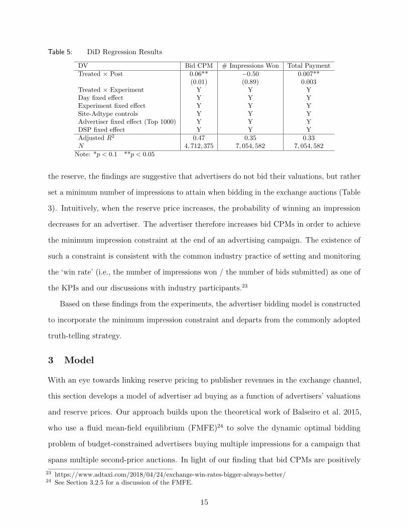
Table 5: DiD Regression Results

DV Bid CPM # Impressions Won Total PaymentTreated × Post 0.06** −0.50 0.007**

(0.01) (0.89) 0.003Treated × Experiment Y Y YDay fixed effect Y Y YExperiment fixed effect Y Y YSite-Adtype controls Y Y YAdvertiser fixed effect (Top 1000) Y Y YDSP fixed effect Y Y YAdjusted R2 0.47 0.35 0.33N 4, 712, 375 7, 054, 582 7, 054, 582

Note: *p < 0.1 **p < 0.05

the reserve, the findings are suggestive that advertisers do not bid their valuations, but rather

set a minimum number of impressions to attain when bidding in the exchange auctions (Table

3). Intuitively, when the reserve price increases, the probability of winning an impression

decreases for an advertiser. The advertiser therefore increases bid CPMs in order to achieve

the minimum impression constraint at the end of an advertising campaign. The existence of

such a constraint is consistent with the common industry practice of setting and monitoring

the ‘win rate’ (i.e., the number of impressions won / the number of bids submitted) as one of

the KPIs and our discussions with industry participants.23

Based on these findings from the experiments, the advertiser bidding model is constructed

to incorporate the minimum impression constraint and departs from the commonly adopted

truth-telling strategy.

3 Model

With an eye towards linking reserve pricing to publisher revenues in the exchange channel,

this section develops a model of advertiser ad buying as a function of advertisers’ valuations

and reserve prices. Our approach builds upon the theoretical work of Balseiro et al. 2015,

who use a fluid mean-field equilibrium (FMFE)24 to solve the dynamic optimal bidding

problem of budget-constrained advertisers buying multiple impressions for a campaign that

spans multiple second-price auctions. In light of our finding that bid CPMs are positively

23 https://www.adtaxi.com/2018/04/24/exchange-win-rates-bigger-always-better/24 See Section 3.2.5 for a discussion of the FMFE.

15

correlated with the reserve prices, we extend this work to consider a FMFE where advertisers

are assumed to face a minimum impression constraint. Analogous to a budget constraint, a

minimum impression constraint can induce advertiser interactions that influence how reserve

prices affect publisher revenues. As we shall show, this constraint induces advertisers to bid

higher than their true valuations (subject to a participation constraint).

In what follows, we describe the publisher-advertiser game and then solve it. Using

backward induction, we first solve the advertiser’s ad buying problem, and then characterize

the publisher’s reserve pricing problem.

3.1 Model Overview

The advertising game proceeds as follows:

1. Publisher: The publisher is the leader and selects the reserve price in the second-price

auction r, for the unsold inventory from the direct channel. The publisher’s objective

is to maximize the long-run expected revenues from the auctions. The publisher knows

the distribution from which advertisers’ valuations are drawn, but does not know the

realized true value for each particular impression.

2. Advertisers: The advertisers are the followers and decides how much to bid b, based

on the realized valuation v for each given impression and the reserve price r. The

advertisers’ objective is to maximize expected utility (= valuation − cost) from the

auctions given the minimum impression level, y.

3.2 Assumptions

This sub-section outlines the model assumptions used to solve the game.

3.2.1 Auction Rule

Reflecting industry practice, impression auctions are second-price, sealed-bid and this auction

format is set exogenously by the ad exchange. An impression is delivered to the winner who

bids the highest above the reserve price (i.e., the winner’s ad is displayed to the consumer).

If no advertiser bids above the reserve price, the impression remains unsold and is perishable.

16

The winner pays the second highest bid, or the reserve price if the second highest bid falls

below the reserve price.

3.2.2 Independent Private Value (IPV)

Following the independent private value assumption adopted in prior work (e.g., Edelman

et al. 2007, Ostrovsky and Schwarz 2011, Balseiro et al. 2015), advertiser valuations are

assumed to be drawn independently from the conditional distribution FV |Z(v|z), where Z is

observed characteristics. After controlling for these observed covariates, advertiser valuations

are assumed to be independent.25,26

3.2.3 Reserve Price

The reserve price is assumed to be known to all potential bidders (advertisers). In practice,

the reserve price is not announced to the advertisers, but they can infer it from their repeated

auction experience (for example, via machine learning algorithms).27

3.2.4 Utility Function

Advertisers are assumed to have a quasi-linear utility function, where utility is defined as the

sum of the advertiser’s valuations from the impressions won less the total payment for the

impressions.

3.2.5 Fluid Mean-Field Equilibrium (FMFE)

The equilibrium concept we adopt is the fluid mean-field equilibrium (FMFE) as defined

in Balseiro et al. 2015. This equilibrium considers a mean-field approximation (Weintraub

et al. 2008, Iyer et al. 2014) to relax the informational requirements of agents. This FMFE

equilibrium concept considers a stochastic fluid approximation from the revenue management

25 This specification allows for values that are common (affiliated) via the covariate Z. For example, Z maycontain site dummies to capture that site1 is valued more than site2 among the advertisers. Z can alsocontain advertiser dummies to control for the heterogeneity across advertisers.26 Athey and Haile 2002 note that the conditional independence assumption (i.e., whether there is unobservedauction-specific heterogeneity after controlling for Z) can be tested if more than one bid is observed ineach auction or the transaction price is observed in auctions with exogenously varying numbers of bidders(Theorem 3). Using the payment data alone, unfortunately, this conditional independence assumption cannotbe tested.27 https://www.aarki.com/blog/understanding-hard-and-soft-price-floors-in-programmatic-media-buying

17

literature that is suitable when the number of bidding opportunities is large (Gallego and

Van Ryzin 1994). In a setting where a large number of advertisers compete, the rational

expectation of competitors’ bids can be formulated (approximated) based on the aggregate

and stationary distribution of others’ bids instead of tracking each individual competitor’s bid.

The FMFE has two benefits. First, it lightens the assumed burden on part of the decision

maker, who needs only to know the distribution of others’ bids (as opposed to all others’

bids). In large markets, tracking all others’ bids would be challenging, if not impossible, for

bidders. Second, this approach reduces the computational burden of solving for a market

equilibrium.28

To employ the FMFE concept, therefore, several assumptions are required. First, the

distribution of competitors’ bids is assumed to be stationary, conditional on the observed

characteristics Z (which includes time dummies) and the reserve price r. Second, the bids of

a single advertiser do not affect this distribution. Given that a large number of advertisers

compete in the exchange channel, and the marginal impact of any player is small, neither of

these assumptions appear restrictive.29

Third, bidders’ minimum impression constraints need only be satisfied in expectation

when bidders solve for their optimal bidding strategies.30 With this third assumption, it

can be shown that bidding strategies that do not condition on the individual state of other

advertisers’ valuations (instead depending only on the bidder’s own valuation, the distribution

of others’ valuations, and the reserve) closely approximate the solution to the optimal bidding

strategy that specifically conditions on the individual states of others. This third assumption

is motivated by the fact that an advertiser has a large number of bidding opportunities over

the campaign length.

28 Readers are referred to Balseiro et al. 2015 for more detail and a formal definition of the FMFE. The authorsalso provide a theoretical justification for using the FMFE as an approximation of advertisers’ behaviors indisplay markets.29 This assumption doesn’t require that the average number of bidders per auction to be large.30 That is, when solving the bidding strategy to maximize its expected utility, the advertiser chooses a biddingfunction that satisfies the minimum impression constraint ex ante, in expectation.

18

3.3 Advertiser Bidding Model

The goal of the advertiser bidding model is to determine the optimal bidding policy faced

by advertisers (which we can match to the data in order to back out the distribution of

advertiser valuations in order to explore the effect of reserves).

The amount of advertising inventory varies over time. Following Balseiro et al. 2015, we

assume that the arrival process of available advertising impressions (' users) at any given

point in time follows a Poisson distribution with intensity η. As suggested in sub-section

2.4.5, we allow for advertiser k to have a minimum impression level yk for the campaign

length sk (i.e., the duration over which an advertiser is using its bidding rule). Then, ηsk

(the expected arrivals times the duration of the bidding interval) indicates the total number

of impressions arriving during the campaign period.

For a given impression i that arrives in this bidding interval (campaign length), we denote

advertiser k’s value as vik, which is assumed to be drawn independently and identically from

a continuous cumulative distribution FV (·|Z). Z are observed characteristics (e.g., ad type).

Further, let D be the steady-state maximum of the competitors’ bids, where the publisher is

also considered as one competitor that submits a bid equal to r. The distribution of D will

endogenously be determined in equilibrium, which we denote as FD.

The advertiser maximizes its expected utility (= valuation − cost) from the ad auctions,

given the minimum impression constraint and the participation constraint. With the

assumptions made in sub-section 3.2, we focus on the bidding strategy βFθ (vi|FD, θ) for

an advertiser type θ = (s, y) (where advertiser type is defined by the campaign length and

the minimum impression level) to be a function of the advertiser’s own valuation vi. The

advertiser faces the optimization problem given by

JFθ (FD) = maxbηsθEV,D [1 {b(V ) ≥ D} (V −D)] (1)

s.t. yθ ≤ ηsθEV,D [1 {b(V ) ≥ D}]

0 ≤ ηsθEV,D [1 {b(V ) ≥ D} (V −D)]

where the expectation is taken over both FV (the distribution of valuations) and FD (the

19

distribution of the maximum competing bid). To define a well-behaved optimization problem,

we assume yk<ηsk , that is the minimum impression level is lower than the total available

impressions.

In the first line, ηsθ indicates the total number of impressions arriving during the campaign

period. 1 {b(V ) ≥ D} indicates the probability of winning the auction on a given arrival,

where the advertiser’s bid is higher than the maximum of the competitors’ bids. Lastly,

(V −D) indicates valuation minus payment, where the payment is consistent with the

second-price rule.

In the second line, the right hand side is the expected number of impressions won at the

end of the campaign period. The inequality constraint assures that the expected number

of impressions won is greater than the minimum impression level yθ. This inequality can

also be written as yθηsθ≤ EV,D [1 {b(V ) ≥ D}], implying that the advertiser tries to attain a

minimum auction winning rate of yθηsθ

.

The third line captures the advertiser’s participation constraint that its expected utility

in bidding in the exchange channel is greater than zero. Below we characterize advertisers’

optimal bidding strategies, assuming that the participation constraints hold (do not bind) in

equilibrium. In sub-section 3.4, we discuss how the participation constraint is imposed in

calculating the optimal reserve price.31

Proposition 1. Suppose that E [D] < ∞ . An optimal bidding strategy that solves (1) is

given by

βFθ (v|FD) = v + µ∗

where µ∗ is the optimal solution of the dual problem

infµ≥0 ηsθEV,D [1 {V ≥ D − µ} (V −D + µ)]− µyθ31 In estimation, where advertiser valuations are inferred conditional on observing the data, this assumptionimplies that the participation constraints do not bind for those observed advertisers at their observed (optimal)bidding strategies given r = 0. This assumption that the participation constraint does not bind in estimationis not restrictive, as it implies that advertisers who participated in the exchange auctions expected to gainpositive utilities at r = 0. In the counterfactual, where we calculate the optimal reserve price, advertisersmight face binding participation constraints as the reserve price increases, thereby potentially dropping outof the auction.

20

That is the advertiser bids higher than its own valuation by a constant factor µ∗, which is

the optimal dual (Lagrangian) multiplier of the minimum impression constraint. Intuitively,

this means that the advertiser foregoes some utility to satisfy the constraint. This constant

factor µ∗ guarantees that the advertiser meets the minimum impression constraint at the end

of the campaign period. Of note, the dynamic nature of the repeated auctions is captured by

this constant factor µ∗, and the bidding strategy becomes static in the sense that µ∗ does not

depend on the current single auction-specific state.32

Proposition 2. If the participation constraints do not bind in equilibrium, the equilibrium

can be characterized as follows:

βFθ (v|FD) = v + µ∗

where µ∗ is µ∗ = 0 if yθ < ηsθEV,D [1 {V ≥ D}]

yθ − ηsθEV,D [1 {V + µ∗ ≥ D}] = 0 if yθ ≥ ηsθEV,D [1 {V ≥ D}]

The proposition states that if the minimum impression constraint is not binding, then

in equilibrium advertisers will bid truthfully (µ∗ = 0). On the other hand, if the minimum

impression constraint does bind, then advertisers will bid higher than the true valuations,

where µ∗ solves the implicit function yθ − ηsθEV,D [1 {V + µ∗ ≥ D}] = 0. Of note, yθ −

ηsθEV,D [1 {V + µ∗ ≥ D}] is the number of expected impressions shy of the minimum impression

level at the end of the campaign, when the optimal bid function is employed.

Based on this proposition, the cost of the minimum impression constraint, µ∗, increases

with the minimum impression level (yθ), and decreases with the number of impressions and

length of campaign (ηsθ). Perhaps more importantly for our purposes, an increase in the

second highest payment, D, lowers EV,D [1 {V + µ∗ ≥ D}] and thus increases µ∗, the bid

premium. Because an increase in reserves can increase D when the reserve binds (it binds

32 In the budget constraint case (Balseiro et al. 2015), advertisers will shade down theirs bids by a constantfactor to account for the future bidding opportunities (future value). In our minimum impression constraintcase, advertisers shade up by this constant factor µ∗ to satisfy the constraint at the end of the campaignperiod.

21

when the second highest valuation is lower than the reserve), reserves can lead to higher bids,

consistent with our experimental data. The proofs for Proposition 1 and Proposition 2 are in

online Appendix B.1.

The primitives to be estimated are (FV , FD, µ) given the reserve price r.

3.4 Optimal Publisher Ad Auction Reserve Price

The publisher’s objective is to maximize the long-run expected revenues from the auctions

given advertiser valuations. Within the independent private value (IPV) paradigm, the

publisher can maximize the revenues from the RTB auctions by choosing the reserve price

optimally.

3.4.1 Publisher’s Optimization Problem

We denote Gθ (µ, r) = EV,D [1 {V + µθ ≥ D}D] to be the expected payment of a θ-type

advertiser when advertisers bid according to the profile µ, and the publisher sets a reserve

price r (Gθ term is the product of the payment times the likelihood the impression is won). We

define I(µ, r) = FD (r|µ) as the probability that the impression is not won in the exchange.

The publisher’s problem can then be written as

maxrη

[∑θ

{pθsθGθ (µ, r)}+ cI(µ, r)

](2)

s.t. µθ ≥ 0 ⊥ yθ ≤ ηsθEV,D [1 {V + µθ ≥ D}] ∀θ ∈ Θ

where pθ is the probability that an arriving advertiser is of type θ and c > 0 is the publisher’s

valuation (i.e., the outside option value if the impression is not won by some advertiser in

the exchange).33

The first term in the sum in the first line indicates the average expenditure of the

advertisers (i.e., the second highest bids when the auctions are won by some advertisers).

The second term in the first line indicates the publisher’s outside option value when the

impression is not won by any advertiser, as it reflects the product of the scrap value of the

impression and the probability the impression is not sold. The constraints in the second line

33 Note that, by definition, I(µ, r) = FD (r|µ) = 1−∑θ {pθsθEV,D [1 {V + µθ ≥ D}]}. Thus, Equation (2)

can be interpreted as the publisher’s value over selling and not selling an impression.

22

reflect the conditions for the Lagrangian multipliers in ensuring the minimum impression

constraints (either the constraint binds or it does not).

3.4.2 Advertiser Participation Constraints

In the counterfactual, where we increase the reserve price to the optimal level, some advertisers

will start to face binding participation constraints as the reserve price increases.34 To

incorporate the effect of the participation constraints in the policy simulation, we ascertain

whether the bidding profile µ satisfies the participation constraint (0 ≤ ηsθEV,D [1 {V + µθ ≥ D} (V −D)])

at the considered reserve price level r for ∀θ ∈ Θ.

In the case the participation constraint does not hold for some advertiser types θ, we

calculate the maximum µθ that satisfies the participation constraint such that

µθ = maxµθ≥0 [0 ≤ ηsθEV,D [1 {V + µθ ≥ D} (V −D)]]

This is, the advertiser increases its bid to v + µθ to bid as closely as possible to its minimum

impression level while satisfying the participation constraint.35

Given the publisher’s outside option value c, the primitives to be recovered from the policy

simulation are the optimal reserve price r∗ and the corresponding outcomes (FV , FD, µ) at

r∗.

4 Identification and Estimation

This sub-section discusses the identification and estimation strategies for the inference of

advertiser valuations.

34 In the extreme case where all advertisers face binding impressions constraints, advertisers’ bidding strategieswill reach ∞ as the reserve price increases to ∞ without the participation constraints.35 Because of the participation constraints, the advertiser may not achieve the minimum impression levelunder the counterfactual. In this case, we are assuming that advertisers purchase as many impressions aspossible toward the minimum impression level while satisfying the participation constraints. Alternatively,we can specify the advertisers to drop-out all together from the exchange channel when the participationconstraints do not meet, but we think the former is more realistic in our context.

23

4.1 Identification

As the publisher currently imposes no reserve price, the identification strategy is described

conditioned on no reserve price.36 First we characterize the identification strategy when

the impression constraint does not bind (µ∗ = 0), then we discuss the case of the binding

constraint (µ∗ > 0).

4.1.1 Case1: µ∗ = 0

The equilibrium-bid function in Proposition 1 implies that advertisers bid truthfully when

the minimum impression constraint does not bind. Thus, the probability density function of

observed bids can directly be mapped to that of valuations. In other words, the distribution

of bids identifies the distribution of valuations such that

f 0V (v) = f 0

B(b)

F 0V (v) = F 0

B(b)

where f 0V and F 0

V (f 0B and F 0

B) represent probability density function and cumulative density

function of valuations (bids) respectively. The superscripts “0” denote the true population

values.

Because only the payment data are used in estimation (see sub-section 2.2), the distribution

of the observed payments needs to be linked to the distribution of valuations. Denoting D to

be the winning payments, F 0D is defined as the distribution of the second highest bids. The

distribution of order statistics implies that

F 0D(v) = n(n− 1)

∫ F 0V (v)

0

un−2(1− u)du

≡ ϕ(F 0V (v)|n

)f 0D(v) = nf 0

v (v)(n− 1)F 0V (v)n−2

(1− F 0

V (v))

In the last line, nf 0v (v) indicates that one of the n advertisers (i.e.,

n

1

= n) draws v

36 When the reserve prices exit, the identification strategy will be similar, but the distribution of bids willrepresent a truncated distribution of valuations due to endogenous participation.

24

exactly, and (n− 1)F 0V (v)n−2 (1− F 0

V (v)) indicates that (n− 2) out of the remaining (n− 1)

advertisers (i.e.,

n− 1

n− 2

= n − 1) draw valuations lower than v, (F 0V (v)n−2), and 1

advertiser draws valuation higher than v, (1− F 0V (v)).

Since ϕ(·|n) is a strictly monotonic function given n, F 0V is identified from the distribution

of observed winning payments F 0D when the number of potential bidders n is known (Paarsch,

Hong, et al. 2006).

4.1.2 Case2: µ∗ > 0

When the minimum impression constraint binds, the distribution of bids identifies the

distribution of valuations up to a location constant µ∗ such that

f 0W (w) = f 0

B(b)

F 0W (w) = F 0

B(b)

where w = v + µ∗ and µ∗ are the optimal Lagrangian multipliers. Thus fW (W ) =

fW (v + µ∗). Assuming we observe the advertiser type θ = (s, y), µ∗ can be estimated

from the conditions in Proposition 2, such that µ∗ solves yθ − ηsθEV,D [1 {V + µ∗θ ≥ D}] = 0

if yθ ≥ ηsθEV,D [1 {V ≥ D}].

Combining the argument in Case 1, F 0V is identified from the distribution of observed

winning payments F 0D, when the number of potential bidders n and the advertiser types (i.e.,

minimum impression level, campaign duration) are known.

4.2 Estimation

The estimation strategy is detailed in this subsection. As in the preceding section, we discuss

the case when the constraint does not bind (µ∗ = 0) first, then incorporate the case of the

binding constraint (µ∗ > 0).

25

4.2.1 Case1: µ∗ = 0

Under the truth-telling scenario, F 0D can be estimated by substituting the sample analogue

for the population quantity as

FD(v) =1

T

T∑t=1

1 [dt ≤ v] (3)

= n(n− 1)

∫ FV (v)

0

un−2(1− u)du

The asymptotic properties of the estimator FD(v) (and the resulting FV ) are discussed in

Paarsch, Hong, et al. 2006.

Incorporating (discrete) covariates is possible as follows. For a given characteristic z ∈ Z,

the estimator of F 0V |Z(v|z) is specified as

FD|Z(v|z) = n(n− 1)

∫ FV |Z(v|z)

0

un−2(1− u)du (4)

Because the number of participants vary across auctions, n-specific non-parametric empirical

cumulative distribution functions (ECDFs) are estimated first for a particular combination

of the z (by n-specific, we mean an ECDF is inferred separately for each auctions with

n bidders). Then FV |Z(v|z) is obtained by kernel smoothing across the n-specific ECDFs

to obtain a single ECDF. The exceptionally large number of payments observed given a

particular combination of ad characteristics facilitates inference in this context of display ad

markets.37

4.2.2 Case2: µ∗ > 0

The key to incorporating the minimum impression constraint is estimating FV |Z together

with µ∗ for a given z. To simplify notation, we drop the dependence on z. The estimation

is done in two stages. In the first stage, we estimate location shifted distribution F 0V (w)

where w = v + µ. In the second stage, conditioned on the recovered distribution F 0V (w), µ is

37 The observed characteristics affecting the valuation are discrete in our context, such as site, ad type (adlocation, ad size, device), and time (month). Although the dimension of Z considered is large, we alsohave many observations per given particular combination of Z, enabling non-parametric estimation. If thecovariates are continuous, semi-parametric approaches such as single-index models (e.g., the density-weightedderivative estimator in Powell et al. 1989, the maximum rank-correlation estimator in Han 1987) can insteadbe used to reduce the curse of dimensionality.

26

estimated using the condition in Proposition 2.

One challenge in estimating valuations when the impression constraint binds is that D, the

distribution of maximum of competing bids, is a function of others’ bids. As such, advertisers

need to form beliefs about the bids of other advertisers. In estimation, this maximum is

observed and equivalent to the rational expectation of the advertisers’ regarding the maximum

of the competitors’ bids. The estimation procedure is outlined in the online Appendix C.1.

4.3 Institutional Details

This sub-section discusses four institutional aspects of the data that warrant additional

attention: (i) metrics (e.g., payments, number of impressions won) are only available as daily

averages instead of at the auction (impression) level, (ii) the number of potential bidders, n,

are not directly observed, (iii) how the minimum impression level and campaign lengths are

operationalized, and (iv) which data points are included in Z.

Daily Aggregate Data The metrics (e.g., payments, # impressions won) provided by the

ad exchange are aggregated to day level, and are not available to this or other publishers at

more granular levels. More specifically, an observational unit in the exchange data represents

total payments, number of impressions won, and number of clicks attained for each given

advertiser-DSP-day-site-ad type. For each observational unit, the average (daily) CPM paid

is calculated as (total payments / number of impressions won). This average (daily) CPM

paid is used as dt in Equation (3) in forming the estimator for FD(v).

As each observation represents a different number of impressions won, we weigh the

average CPM paid by the number of impressions won when estimating the distribution of

valuations. That is, a data point (y average CPM paid, x number of impressions won) is

treated as if there are x number of observations with y CPM payment.38

38 The magnitude of the potential bias in using the aggregate data (as opposed to the impression level data)is to be examined. Our conjecture is that the variance of the valuation distribution will be biased downwardwhen using the aggregate data, but its impact on the optimal reserve price level will be small (or minimal).We will provide a formal analysis at a later time.

27

Number of Potential Bidders The identification strategy discussed above requires that

the number of potential bidders n is known. The number of potential bidders for a given

observational unit (advertiser-DSP-day-site-ad type) will be

n = n1(# advertisers with CPM payment, i.e., positive # impressions won)

+ n2(# advertisers with bids submitted, but zero impressions won)

n1 is observed in the data, while n2 is observed only for the opt-in advertisers. Thus, to

operationalize n, we use the the following proxy:39

n = n1(# advertisers with CPM payment, i.e., positive # impressions won)

+ n2,opt−in(# opt-in advertisers with bids submitted, but zero impressions won)

Minimum Impression Level and Campaign Length When advertisers do not face

binding minimum impression constraints, advertisers bid truthfully and the distribution

of valuations can be recovered without the knowledge of the minimum impression level

or the campaign length. In the case the minimum impression constraints bind for some

advertisers, the identification strategy discussed in sub-section 4.1.2 requires more information

from the researcher. More specifically, in forming the estimator in Equation (10) in the

online Appendix, τθ =(yθηsθ

)term is required as an input. This term reflects the minimum

winning rate the advertiser aims to attain for a given impression for a campaign. Thus, τθ is

advertiser-campaign specific. In the estimation (and the counterfactual), we allow τ to vary

across advertisers, but hold constant the minimum winning rate within an advertiser across

campaigns. Denoting k to be the advertiser, τk is proxied by

τk = min (Ik1, ...Ikm, ...IkM) , Ikm > 0 ∀m

Ikm =1∑

day∈m 1 [ik,day > 0]uday

∑day∈m

ik,day

where ik,day represents the impressions won by advertiser k and uday represents the impressions

available for sale on a given day. Ikm in the second line constructs the winning rate for a

39 n2,opt−out will be small for two reasons. First, 82% of advertisers opted-in to share their bidding information(default setting). Second, the opt-out advertisers (18%) constitute about 84% of the total revenues, meaningopt-out advertisers are highly likely to be included in n1, which is observed.

28

given month m, conditional on participating in the exchange. In other words, τk is computed

as the minimum of the monthly winning rates observed in the data, conditioned on the

advertiser participating in the exchange. Accordingly, the optimal bidding strategy profile

µ|Z, is recovered at the advertiser level, instead of advertiser-campaign level.40

The solution to the publisher’s optimal reserve price in Equation (2) also involves the term

δθ = pθsθ which represents the share of each advertiser’s type present in the auction (where

type θ is uniquely defined by a campaign length and a minimum impression level). This share

of advertiser types is determined by the product of the advertiser type’s arrival probability,

pθ, and the campaign duration, sθ; this product represents the fraction of advertisers in

an auction that play bidding strategy profile µθ. We do not observe pθ and sθ, but can

nonetheless compute δθ at the advertiser-type level (that is, setting θ = k). We do this by

approximating the weight for each advertiser by its observed share of participation. Thus, we

use below proxy for δθ=k

δk|Z =

∑day 1 [ik,day > 0]∑

k

∑day 1 [ik,day > 0]

where ik,day represents the impressions won by advertiser k on a given day. 1 [ik,day > 0] takes

value 1 if the advertiser k wins a positive amount of impressions on a given day. We include

‘month’ as the observable characteristics in Z, so the summation is done over days within

a month. This δk|Z is the weight advertiser k (with the bidding strategy profile µk) plays

toward the platform’s revenue given Z.

Observed Covariates The distribution of valuations is estimated separately for each

combination of Zs to control for heterogeneity. The observed covariates considered in Z are

• Site: 20 U.S. based sites are considered.

• Ad location: these include above-the-fold (ATF), MID, below-the-fold (BTF), and no

40 The identification strategy discussed in subsection 4.1 relies solely upon the observational data. Altenatively,one could leverage the experimental data (i.e., the causal change in bid CPMs) to impute the minimumimpression level. Specifically, the optimiality condition in Proposition 2 implies a one-to-one mapping betweeni) the minimum impression level and ii) the causal change in bid CPM in the experimental data. However,our identification strategy based on the observational data enables us to (i) recommend optimal pricingschemes for those sites upon which we have not conducted experiments and to (ii) reserve experimental datafor providing a validation for our model.

29

information available.

• Ad size: are represented by 300x250, (728x90, 970x66), 320x50, and 300x600. These

are the sizes conforming to Interactive Advertising Bureau (IAB) standard guideline

and are most commonly used by the advertisers.41

• Device: the various devices include desktop, mobile, and tablet.

• Month: controls are included for seasonality.

In sum, we estimate the distribution of valuations for each 11, 520 (20x4x4x3x12) combination

of Zs.42

5 Results

This section outlines the advertiser bidding model results used to infer the advertiser valuation

distribution. Recall, estimation recovers i) the distribution of the underlying advertiser

valuations FV , and ii) the vector of optimal Lagrangian multipliers µ∗ = (µ∗1, .., µ∗θ, ..µ

∗Θ)

which reflects the tightness of the advertisers’ minimum impression constraints. The

pair (FV ,µ∗) is obtained for each combination of observables Z (discrete space of site-ad

location-ad size-device-month). Below we report the estimates for the treatment groups in

the experimental data in the month prior to the experiment (09/2017).

5.1 The Valuation Distribution, FV

The cumulative density function of the advertiser valuations, Fv, is plotted in Figure 5 for

Experiment 1. The cdf of the advertiser valuations (FV , blue line) is recovered from the

observed payments (FD, red line).43 This figure shows how valuations exceed payments. For

example, about 40% of advertisers have a valuation of less than $2.00, and 60% of advertisers

pay less than $2.00.

41 https://www.iab.com/guidelines/42 Advertiser (or DSP)-specific distribution of valuations will be explored in the future to control for theheterogeneity across advertisers (or DSPs).43 The recovered cdf of the advertiser valuations for all experiments are included in Figure 8 in onlineAppendix.

30

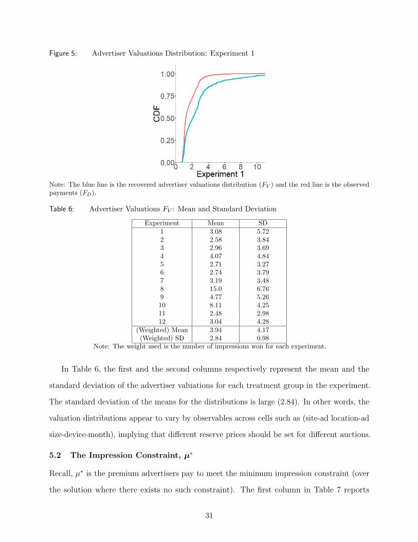
Figure 5: Advertiser Valuations Distribution: Experiment 1

Note: The blue line is the recovered advertiser valuations distribution (FV ) and the red line is the observedpayments (FD).

Table 6: Advertiser Valuations FV : Mean and Standard Deviation

Experiment Mean SD1 3.08 5.722 2.58 3.843 2.96 3.694 4.07 4.845 2.71 3.276 2.74 3.797 3.19 3.488 15.0 6.769 4.77 5.2610 8.11 4.2511 2.48 2.9812 3.04 4.28

(Weighted) Mean 3.94 4.17(Weighted) SD 2.84 0.98

Note: The weight used is the number of impressions won for each experiment.

In Table 6, the first and the second columns respectively represent the mean and the

standard deviation of the advertiser valuations for each treatment group in the experiment.

The standard deviation of the means for the distributions is large (2.84). In other words, the

valuation distributions appear to vary by observables across cells such as (site-ad location-ad

size-device-month), implying that different reserve prices should be set for different auctions.

5.2 The Impression Constraint, µ∗

Recall, µ∗ is the premium advertisers pay to meet the minimum impression constraint (over

the solution where there exists no such constraint). The first column in Table 7 reports

31

the percentage of advertisers bound by the minimum impression constraint (i.e., those with

positive Lagrangian multipliers µk∗ > 0) at r = 0. On average, about 19% of the advertisers

face binding minimum impression constraints during the prior experimental period when

r = 0. Moreover, as the average advertiser valuation for an impression is about $3.94, a

“back of the envelope” calculation suggests that advertisers bid around 20% (0.78/3.94) higher

than their true valuations because of the binding minimum impression constraint when there

is no reserve, r = 0. Also of note, the standard deviations of µ are high (see fifth column in

Table 7), meaning the cost of the constraint varies significantly across advertisers.

The percent of advertisers bound by the constraint increases from 19 to 32 as the publisher

increases the reserve prices. As a result, the cost of the constraint increases from $0.78 to

$0.99 and the overall cost of the constraint across advertisers grows substantially, from 20%

to 25%.

Table 7: The Impression Constraint, µ∗

Experiment % Advertisers Constrained µ: Mean µ: SDr = 0 r∗ r = 0 r∗ r = 0 r∗

1 19.0 33.5 0.66 0.77 4.68 3.332 15.3 36.1 0.54 0.96 2.54 3.513 17.1 35.8 0.62 1.08 2.27 3.884 17.4 22.0 0.93 0.97 3.45 3.425 27.8 38.4 0.72 0.78 15.3 15.36 26.1 56.4 0.43 0.52 5.53 5.397 19.4 26.5 0.88 0.90 5.51 3.858 9.19 9.2 1.26 1.35 5.87 5.809 21.4 45.9 1.34 1.85 5.63 5.5910 18.2 17.7 1.27 1.43 3.06 3.9211 16.7 37.5 0.62 1.08 2.70 3.5512 26.1 55.1 0.79 0.91 11.1 10.9

(Weighted) Mean 18.7 31.7 0.78 0.99 4.94 5.07(Weighted) SD 4.35 10.7 0.24 0.22 3.91 3.66

6 Setting Reserve Prices

In this section, we compute the optimal reserve price to maximize the publisher’s revenues in

the ad exchange auctions. Based on the recovered advertiser distribution FV , the optimal

reserve can be obtained by solving the publisher’s optimization problem prescribed in Equation

(2).

32

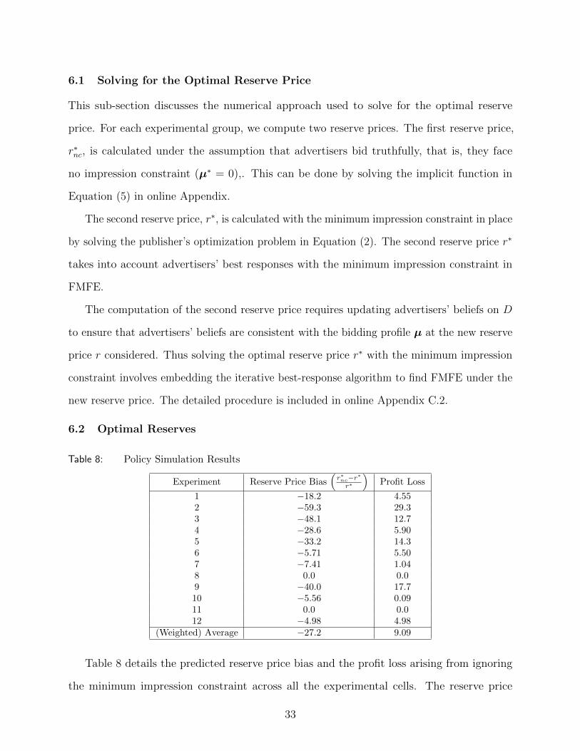
6.1 Solving for the Optimal Reserve Price

This sub-section discusses the numerical approach used to solve for the optimal reserve

price. For each experimental group, we compute two reserve prices. The first reserve price,

r∗nc, is calculated under the assumption that advertisers bid truthfully, that is, they face

no impression constraint (µ∗ = 0),. This can be done by solving the implicit function in

Equation (5) in online Appendix.

The second reserve price, r∗, is calculated with the minimum impression constraint in place

by solving the publisher’s optimization problem in Equation (2). The second reserve price r∗

takes into account advertisers’ best responses with the minimum impression constraint in

FMFE.

The computation of the second reserve price requires updating advertisers’ beliefs on D

to ensure that advertisers’ beliefs are consistent with the bidding profile µ at the new reserve

price r considered. Thus solving the optimal reserve price r∗ with the minimum impression

constraint involves embedding the iterative best-response algorithm to find FMFE under the

new reserve price. The detailed procedure is included in online Appendix C.2.

6.2 Optimal Reserves

Table 8: Policy Simulation Results

Experiment Reserve Price Bias(r∗nc−r

∗

r∗

)Profit Loss

1 −18.2 4.552 −59.3 29.33 −48.1 12.74 −28.6 5.905 −33.2 14.36 −5.71 5.507 −7.41 1.048 0.0 0.09 −40.0 17.710 −5.56 0.0911 0.0 0.012 −4.98 4.98

(Weighted) Average −27.2 9.09

Table 8 details the predicted reserve price bias and the profit loss arising from ignoring

the minimum impression constraint across all the experimental cells. The reserve price

33

bias is calculated as the (optimal reserve without the constraint - optimal reserve with

the constraint)÷(optimal reserve with the constraint). The profit loss is calculated as the

difference in profits when setting the optimal reserve with the constraint and without. On

average, the optimal reserve price calculated with no constraint is about 27% lower than

the optimal reserve calculated with the minimum impression constraint, but can be as high

as 59%. Further, the profit loss in ignoring this constraint is calculated to be around 9%

across experiments, but can be as high as 29%. From this, we conclude that the minimum

impression constraint can lead to even more substantial gains in publisher revenues than a

naive approach that assumes no constraint.

7 Conclusion

With the rapid growth in display advertising markets, there is an increasing value in

characterizing the advertisers’ valuations for ad impressions, and how advertiser strategies

are affected by practical constraints (such as reach or budget) or by the reserve price in

advertising exchange markets. Taking the perspective of the publisher, we consider how

reserve prices should be set for auctions when selling display advertising impressions through

these ad exchanges.

The optimal reserve is a function of advertiser valuations, and auction theory has

established that bidding one’s true valuation is the weakly dominant strategy in static,

second-price, sealed-bid auction with standard assumptions. Though the one-shot game

setting is tractable and often adopted in models of advertiser bidding (e.g., Sayedi 2018, Celis

et al. 2014, Johnson 2013), our discussions with industry participants indicate that advertisers

recognize that they buy multiple impressions across multiple auctions with some constraints

on reach or budget. This implies that advertisers view ad buying as playing repeated games

with some constraints, which would then lead their bids to deviate from truth-telling.

In a series of experiments, setting the reserve price under the assumption advertisers play

a one-shot game without any constraints is shown to increase publisher’s revenue substantially,

by 32% (notably, at no additional cost to the publisher). By manipulating the reserve in this

34

fashion, we test the extent to which reach or budget constraints (across multiple auctions)

affect advertisers’ bidding behaviors. Experimental findings indicate that increasing the

reserve price increases advertisers’ bid CPMs and total payments, while it does not have an

impact on the total number of impressions won by the advertisers. We show these patterns

are most consistent with advertisers playing repeated auctions with minimum impression

constraint.

Subsequently, we construct an advertiser bidding model that incorporates the minimum

impression constraint. The model builds on the notion of a fluid mean-field equilibrium

developed in Balseiro et al. 2015, which well approximates the rational behavior of thousands of

advertisers competing in repeated auctions with some constraints. We extend this theoretical

framework to incorporate the minimum impression constraint, and suggest estimation and

identification strategies in applying it to our empirical context. Our counterfactual results

show that the reserve price solved without imposing the minimum impression constraint is

27% lower than the optimal reserve level with the minimum impression constraint. Because

ignoring the minimum impression constraint biases the solution downward, the profit loss in

ignoring this constraint is found to be about 9%. We plan to conduct an additional set of

experiments to validate this pricing policy.

While this paper addresses a question of growing economic importance with a novel

dataset, a number of additional extensions are possible. In particular, publishers often sell

advertising inventory via direct sales as well as RTB. Direct selling involves advance sale of a

bundle of impressions directly to the advertiser at a fixed price. Extending our research to

consider optimal joint pricing (e.g., fixed price in the direct, reserve price in the ad exchange),

and whether inventory should first be made available to one channel or another, are interesting

directions for future research.44 A second question of interest is motivated by noting that

advertiser valuations are incumbent upon the information available to the advertisers about

44 We consider reserve prices, taking direct sales decisions made as given (e.g., price, number of impressionsbought and sold in direct). Taking the direct channel as given is an assumption that mirrors the structureof the market we consider, where the impressions are sold in the ad exchange after they do not sell in thedirect sales channel. Thus, our solution to the optimal reserve prices can be viewed as the sub-game perfectequilibrium solution to the second-stage, taking the first-stage decisions as given.

35

the impression. This raises the question of whether and how much information a publisher

should share with an exchange.

To the best of our knowledge, this paper is among the first to empirically consider the

issues of pricing in display advertising markets. Given our initial results and the growth in

these markets, we hope this and future research will continue to yield economically meaningful

implications for publishers in these rapidly growing markets and lead to more research in

this area.

36

References

Athey, S., and P. A. Haile. 2002. “Identification of standard auction models.” Econometrica

70 (6): 2107–2140.

Backus, M., and G. Lewis. 2016. Dynamic demand estimation in auction markets. Technical

report. National Bureau of Economic Research.

Bajari, P., and A. Hortacsu. 2003. “The winner’s curse, reserve prices, and endogenous entry:

Empirical insights from eBay auctions.” RAND Journal of Economics: 329–355.

Balseiro, S. R., O. Besbes, and G. Y. Weintraub. 2015. “Repeated auctions with budgets in

ad exchanges: Approximations and design.” Management Science 61 (4): 864–884.

Balseiro, S. R., and Y. Gur. 2019. “Learning in repeated auctions with budgets: Regret

minimization and equilibrium.” Management Science.

Barajas, J., R. Akella, M. Holtan, and A. Flores. 2016. “Experimental designs and estimation

for online display advertising attribution in marketplaces.” Marketing Science 35 (3):

465–483.

Cai, H., K. Ren, W. Zhang, K. Malialis, J. Wang, Y. Yu, and D. Guo. 2017. “Real-time

bidding by reinforcement learning in display advertising.” In Proceedings of the 10th

international conference on web search and data mining, 661–670. ACM.

Celis, L. E., G. Lewis, M. Mobius, and H. Nazerzadeh. 2014. “Buy-it-now or take-a-chance:

Price discrimination through randomized auctions.” Management Science 60 (12):

2927–2948.

Choi, H., C. F. Mela, S. Balseiro, and A. Leary. 2017. “Online Display Advertising Markets:

A Literature Review and Future Directions.” Available at SSRN 3070706.

Edelman, B., M. Ostrovsky, and M. Schwarz. 2007. “Internet advertising and the generalized

second-price auction: Selling billions of dollars worth of keywords.” The American

Economic Review 97 (1): 242–259.

Gallego, G., and G. Van Ryzin. 1994. “Optimal dynamic pricing of inventories with stochastic

demand over finite horizons.” Management science 40 (8): 999–1020.

Ghosh, A., B. Rubinstein, S. Vassilvitskii, and M. Zinkevich. 2009. “Adaptive bidding for

display advertising.” In Proceedings of the 18th international conference on world wide

web, 251–260. ACM.

Goldfarb, A., and C. Tucker. 2011. “Privacy regulation and online advertising.” Management

science 57 (1): 57–71.

Han, A. K. 1987. “Non-parametric analysis of a generalized regression model: the maximum

rank correlation estimator.” Journal of Econometrics 35 (2-3): 303–316.

Hendricks, K., and A. Sorensen. 2015. The role of intermediaries in dynamic auction markets.

Technical report. Working paper, University of Wisconsin.

37

Hoban, P. R., and R. E. Bucklin. 2015. “Effects of internet display advertising in the purchase

funnel: Model-based insights from a randomized field experiment.” Journal of Marketing

Research 52 (3): 375–393.

Hong, H., and M. Shum. 2002. “Increasing competition and the winner’s curse: Evidence

from procurement.” The Review of Economic Studies 69 (4): 871–898.

Iyer, K., R. Johari, and M. Sundararajan. 2014. “Mean field equilibria of dynamic auctions

with learning.” Management Science 60 (12): 2949–2970.

Johnson, G. A. 2013. “The impact of privacy policy on the auction market for online display

advertising.” Working paper.

Johnson, G. A., R. A. Lewis, and E. I. Nubbemeyer. 2016. “The online display ad effectiveness

funnel & carryover: A meta-study of predicted ghost ad experiments.” Working paper.

Johnson, G. A., R. A. Lewis, and D. Reiley. 2016. “Location, location, location: Repetition

and proximity increase advertising effectiveness.” Working paper.

Krusell, P., and A. A. Smith Jr. 1998. “Income and wealth heterogeneity in the macroeconomy.”

Journal of political Economy 106 (5): 867–896.

Lee, K.-C., A. Jalali, and A. Dasdan. 2013. “Real time bid optimization with smooth budget

delivery in online advertising.” In Proceedings of the 7th international workshop on data

mining for online advertising, 1. ACM.

Lewis, R. A., and J. M. Rao. 2015. “The unfavorable economics of measuring the returns to

advertising.” The Quarterly Journal of Economics 130 (4): 1941–1973.

Ostrovsky, M., and M. Schwarz. 2011. “Reserve prices in internet advertising auctions: A

field experiment.” In Proceedings of the 12th conference on electronic commerce, 59–60.

ACM.

Paarsch, H. J., H. Hong, et al. 2006. “An introduction to the structural econometrics of

auction data.” MIT Press Books 1.

Powell, J. L., J. H. Stock, and T. M. Stoker. 1989. “Semiparametric estimation of index

coefficients.” Econometrica: Journal of the Econometric Society: 1403–1430.

Rafieian, O., and H. Yoganarasimhan. 2016. “The value of information in mobile ad targeting.”

Working paper.

Riley, J. G., and W. F. Samuelson. 1981. “Optimal auctions.” The American Economic

Review 71 (3): 381–392.

Sahni, N. S. 2015. “Effect of temporal spacing between advertising exposures: Evidence from

online field experiments.” Quantitative Marketing and Economics 13 (3): 203–247.

Sayedi, A. 2018. “Real-time bidding in online display advertising.” Marketing Science 37 (4):

553–568.

38

Tucker, C. 2014. “Social networks, personalized advertising, and privacy controls.” Journal

of Marketing Research 51 (5): 546–562.

Weintraub, G. Y., C. L. Benkard, and B. Van Roy. 2008. “Markov perfect industry dynamics

with many firms.” Econometrica 76 (6): 1375–1411.

Xu, J., K.-c. Lee, W. Li, H. Qi, and Q. Lu. 2015. “Smart pacing for effective online ad campaign

optimization.” In Proceedings of the 21th international conference on knowledge discovery

and data mining, 2217–2226. ACM.

Yuan, S., J. Wang, and X. Zhao. 2013. “Real-time bidding for online advertising: Measurement

and analysis.” In Proceedings of the 7th international workshop on data mining for online

advertising, 3. ACM.

39

Online Appendix

A Field Experiment

A.1 Experiment Design

A series of experiments were designed to manipulate the reserve prices in the exchange channel.

Data were collected for the period 08/01/2017 - 12/03/2017, where 08/01/2017 - 10/15/2017

constitute the ‘Prior’ period and 10/19/2017 - 12/03/2017 constitute the ‘Post’ period where

the changes in reserve prices took place for the treatment group. The experiments were

conducted on two chosen websites that were closest in terms of contents, user demographics,

revenues, and number of impressions (user visits).

A.1.1 Treatment and Control Groups

The experiments were designed to run across different ad types including (i) site (site1 and

site2), (i) device (desktop, mobile, tablet, no info), (iii) ad location (ATF, MID, BTF, no

info, front door), and (iv) size (300x250, 728x90, 970x66, 320x50, 300x600, 970x250). Twelve

experiments were constructed; each constituted a pair, closest in ad characteristics, that was

randomized either into the treatment or the control group. For example, (site1, desktop,

BTF, 300x250) and (site1, desktop, ATF, 300x250) were paired for the first experiment, and

the randomly chosen (site1, desktop, BTF, 300x250) was assigned to the treatment group,

whereas (site1, desktop, ATF, 300x250) was assigned to the control group. Table 9 shows the

full list of the experiments and the corresponding treatment and control group characteristics.

Table 9: Treatment and Control Groups

Id Device Site and Position Inventory SizeTreatment Control Treatment Control

1 Desktop Site1 BTF Site1 ATF 300x250 300x2502 Desktop Site2 MID Site2 ATF, BTF 300x250 300x2503 Mobile Site1 No Info Site2 MID, BTF 300x250 300x2504 Mobile Site2 ATF Site2 MID, BTF 300x250 300x2505 Desktop Site1 ATF Site1 BTF 728x90, 970x66 728x90, 970x666 Tablet Site1 ATF, BTF Site1 No Info 728x90, 970x66 728x90, 970x667 Mobile Site2 MID, BTF Site1 No Info, Site2 ATF 320x50 320x508 Desktop Site1 ATF Site2 ATF 300x600 300x6009 All Site1 Front Door BTF Site1 Front Door BTF 300x250 728x9010 Desktop Site1 ATF Site1 BTF 970x250 970x25011 Tablet Site1 No Info Site2 ATF, MID, BTF 300x250 300x25012 Desktop Site2 BTF Site2 ATF 728x90, 970x66 728x90, 970x66

A.1.2 Optimal Reserve Price

For purposes of the experiment, advertiser valuations are estimated assuming advertisers

use truth-telling strategies, and the optimal reserve prices are calculated conditioned on this

1

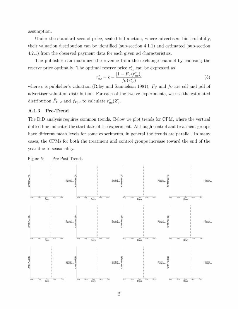
assumption.

Under the standard second-price, sealed-bid auction, where advertisers bid truthfully,

their valuation distribution can be identified (sub-section 4.1.1) and estimated (sub-section

4.2.1) from the observed payment data for each given ad characteristics.

The publisher can maximize the revenue from the exchange channel by choosing the

reserve price optimally. The optimal reserve price r∗nc can be expressed as

r∗nc = c+[1− FV (r∗nc)]

fV (r∗nc)(5)

where c is publisher’s valuation (Riley and Samuelson 1981). FV and fV are cdf and pdf of

advertiser valuation distribution. For each of the twelve experiments, we use the estimated

distribution FV |Z and fV |Z to calculate r∗nc(Z).

A.1.3 Pre-Trend

The DiD analysis requires common trends. Below we plot trends for CPM, where the vertical

dotted line indicates the start date of the experiment. Although control and treatment groups

have different mean levels for some experiments, in general the trends are parallel. In many

cases, the CPMs for both the treatment and control groups increase toward the end of the

year due to seasonality.

Figure 6: Pre-Post Trends

Aug Sep Oct Nov DecDays

CP

M P

aid

($)

ControlTreatment

Aug Sep Oct Nov DecDays

CP

M P

aid

($)

ControlTreatment

Aug Sep Oct Nov DecDays

CP

M P

aid

($)

ControlTreatment

Aug Sep Oct Nov DecDays

CP

M P

aid

($)

ControlTreatment

Aug Sep Oct Nov DecDays

CP

M P

aid

($)

ControlTreatment

Aug Sep Oct Nov DecDays

CP

M P

aid

($)

ControlTreatment

Aug Sep Oct Nov DecDays

CP

M P

aid

($)

ControlTreatment

Aug Sep Oct Nov DecDays

CP

M P

aid

($)

ControlTreatment

Aug Sep Oct Nov DecDays

CP

M P

aid

($)

ControlTreatment

Aug Sep Oct Nov DecDays

CP

M P

aid

($)

ControlTreatment

Aug Sep Oct Nov DecDays

CP

M P

aid

($)

ControlTreatment

Aug Sep Oct Nov DecDays

CP

M P

aid

($)

ControlTreatment

2

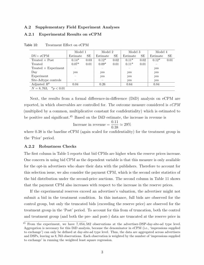
A.2 Supplementary Field Experiment Analyses

A.2.1 Experimental Results on eCPM

Table 10: Treatment Effect on eCPM

Model 1 Model 2 Model 3 Model 4DV= eCPM Estimate SE Estimate SE Estimate SE Estimate SETreated × Post 0.14* 0.03 0.12* 0.02 0.11* 0.02 0.12* 0.01Treated 0.07* 0.01 0.09* 0.01 0.11* 0.01 –Treated × Experiment – – – yesDay yes yes yes yesExperiment – yes yes yesSite-Adtype controls – – yes yesAdjusted R2 0.04 0.26 0.64 0.84N = 8, 763, *p < 0.01

Next, the results from a formal difference-in-difference (DiD) analysis on eCPM are

reported, in which observables are controlled for. The outcome measure considered is eCPM

(multiplied by a common, multiplicative constant for confidentiality) which is estimated to

be positive and significant.45 Based on the DiD estimate, the increase in revenue is

Increase in revenue =0.11

0.38' 29%

where 0.38 is the baseline eCPM (again scaled for confidentiality) for the treatment group in

the ‘Prior’ period.

A.2.2 Robustness Checks

The first column in Table 5 reports that bid CPMs are higher when the reserve prices increase.

One concern in using bid CPM as the dependent variable is that this measure is only available

for the opt-in advertisers who share their data with the publishers. Therefore to account for

this selection issue, we also consider the payment CPM, which is the second order statistics of

the bid distribution under the second-price auctions. The second column in Table 11 shows

that the payment CPM also increases with respect to the increase in the reserve prices.

If the experimental reserves exceed an advertiser’s valuation, the advertiser might not

submit a bid in the treatment condition. In this instance, full bids are observed for the

control group, but only the truncated bids (exceeding the reserve price) are observed for the

treatment group in the ‘Post’ period. To account for this from of truncation, both the control

and treatment group (and both the pre- and post-) data are truncated at the reserve price in

45 From the experiment, we have 7, 054, 582 observations at the advertiser-DSP-day-site-ad type level.Aggregation is necessary for this DiD analysis, because the denominator in eCPM (i.e., ‘impressions suppliedto exchange’) can only be defined at day-site-ad type level. Thus, the data are aggregated across advertisersand DSPs, leaving us 8, 763 observations. Each observation is weighted by the number of ‘impressions suppliedto exchange’ in running the weighted least square regression.

3

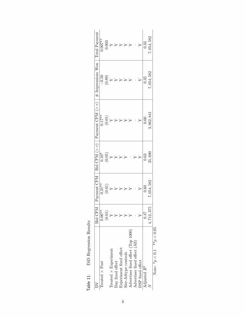
Table

11:

DiD

Reg

ress

ion

Res

ult

s

DV

Bid

CP

MP

aym

ent

CP

MB

idC

PM

(>r)

Pay

men

tC

PM

(>r)

#Im

pre

ssio

ns

Won

Tota

lP

aym

ent

Tre

ated×

Pos

t0.0

6**

0.31**

0.10*

0.1

7**

−0.5

00.0

07**

(0.0

1)(0.0

1)

(0.0

5)

(0.0

1)

(0.8

9)

0.003

Tre

ated×

Exp

erim

ent

YY

YY

YY

Day

fixed

effec

tY

YY

YY

YE

xp

erim

ent

fixed

effec

tY

YY

YY

YS

ite-

Ad

typ

eco

ntr

ols

YY

YY

YY

Ad

vert

iser

fixed

effec

t(T

op10

00)

YY

–Y

YY

Ad

vert

iser

fixed

effec

t(A

ll)

––

Y–

––

DS

Pfi

xed

effec

tY

YY

YY

YA

dju

sted

R2

0.47

0.6

00.6

30.

60

0.35

0.3

3N

4,71

2,3

757,

054,5

82

35,

690

3,062,8

41

7,054,5

82

7,054,5

82

Not

e:*p<

0.1

**p<

0.05

4

the DiD analysis. If advertisers bid their true valuations, bids in this truncated region will

stay the same, pre- and post- the experiments. However, in the third column in Table 11, bid

CPMs increase with the reserve prices.

Similarly, the payment CPM for the treatment group in the ‘Post’ period will, by definition,

be truncated at the reserve price set by the publisher. To account for this effect, we also

run DiD analysis for the payment data conditioned on being above the reserve price (i.e.,

payments are left-truncated at the post period, treatment group reserve level, for both the

control and treatment group and for both the pre- and post-periods). Results are robust

inasmuch as the second-highest bids increase with the reserve prices, conditioned on payments

exceeding the reserve price set for the experiment (the fourth column).

In sum, the result that advertisers bid higher when the publisher increases the reserve

price is robust to various controls, measures, and assumptions.

B Model

B.1 Proofs

B.1.1 Proposition 1

The proof for Proposition 1 follows the steps established in Balseiro et al. 2015 Section

A.1. First, the dual of the primal problem in Equation (1) is introduced using a Lagrange

multiplier for the minimum impression constraint. Second, the first-order conditions are

derived to determine the solution for the dual problem.

Step 1: The Lagrangian for type θ is denoted as

Lθ(b, µ) = ηsθEV,D [1 {b(V ) ≥ D} (V −D)] + µ [ηsθEV,D [1 {b(V ) ≥ D}]− yθ] (6)

= ηsθEV,D [1 {b(V ) ≥ D} (V −D + µ)]− µyθwhere a Lagrange multiplier for the minimum impression constraint is µ ≥ 0. The dual problem

(converting from maximizing the advertiser’s objective function given its minimum impression

constraint in Equation (1) to minimizing the Lagrangian multipliers while maximizing the

objective function) is given by

Ψθ(µ) =infµ≥0supb(·)Lθ(b, µ)

=infµ≥0

{ηsθsupb(·) {EV,D [1 {b(V ) ≥ D} (V + µ−D)]} − µyθ

}(7)

=infµ≥0 {ηsθEV,D [1 {V ≥ D − µ} (V − (D − µ))]− µyθ}

the inf is the Lagrangian minimization step and the sup is the goal maximization step. The

equality in the last line comes from the fact that the inner optimization problem is similar to

an advertiser’s problem who faces value v + µ and seeks to maximize its expected utility in

5

the second-price auction so that bidding truthfully becomes optimal (consider Equation 1

without the constraints). That is for any given multiplier µ ≥ 0, the inner expectation term

is maximized with the policy b(V ) = V + µ. Further, the term within the expectation in the

last line is convex in µ, and the expectation preserves convexity, leading to a convex dual

problem.

Step 2: The first order condition of Ψθ(µ) with respect to µ (that is, the FOC for the

infµ≥0{·}) is given by

(d/dµ)Ψθ(µ) =ηsθEV,D [1 {V ≥ D − µ}]− yθ = 0 (8)

To explain the solution to this FOC, we begin by noting that Ψθ(µ) is convex in µ. If the

constraint does not bind (i.e., ηsθEV,D [1 {V ≥ D}] ≥ yθ), then (d/dµ)Ψθ ≥ 0 at µ = 0. This

condition implies the function Ψθ(µ) is increasing in µ for all µ ≥ 0, such that the function

is minimized at µ∗ = 0 (has a corner solution). Intuitively, the Lagrangian multiplier can

be interpreted as the cost of the impressions constraint; If the constraint does not bind, the

constraint is costless.

On the other hand, when the constraint binds (i.e., the optimal unconstrained number of

impressions is less than the minimum impression level, that is ηsθEV,D [1 {V ≥ D}] < yθ),

then (d/dµ)Ψθ(µ) takes a negative value at µ = 0. As µ→∞, (d/dµ)Ψθ(µ) converges to a

positive value ηsθ − yθ > 0, because limµ→∞EV,D [1 {V ≥ D − µ}] = 1.46 Thus, there exists

a unique interior solution µ∗ > 0 for (d/dµ)Ψθ(µ∗) = 0 as Ψθ is a convex function in µ.

Moreover, the complementary slackness conditions hold with the bidding function b∗(V ) =

βFθ = v + µ∗ and the optimal multiplier µ∗ such that:

µ∗[ηsθEV,D

[1{βFθ (V ) ≥ D

}]− yθ

]= 0,

That is, either i) the minimum impression constraint binds or ii) the Lagrangian multiplier

µ∗ is 0.

Lastly, there is no duality gap. That is, there is no difference between the primal (1) and

dual (7) values. The bid function βFθ is primal feasible from the first-order conditions of the

dual, and the primal objective value calculated at the proposed bid function (b(V ) = βFθ ) is

46 (ηsθ − yθ) is a finite positive number as we constrain ηsθ > yθ when defining the optimization problem insub-section 3.3 (i.e., the minimum impression level is lower than the total available impressions).

6

then

ηsθEV,D[1{βFθ ≥ D

}(V −D)

]=(ηsθEV,D

[1{βFθ ≥ D

}(V −D)

]+ µ∗

[ηsθEV,D

[1{βFθ ≥ D

}]− yθ

])− µ∗

[ηsθEV,D

[1{βFθ ≥ D

}]− yθ

]=Lθ(βFθ , µ∗)− µ∗

[ηsθEV,D

[1{βFθ (V ) ≥ D

}]− yθ

]=Lθ(βFθ , µ∗)

=Ψθ(µ∗)

where the third equality follows from the complementary slackness conditions, as µ = µ∗

is the value for which µ∗[ηsθEV,D

[1{βFθ (V ) ≥ D

}]− yθ

]= 0. Finally, the last equality

follows from the fact that Ψθ(µ∗) = supb(·)Lθ(b, µ∗) and the optimal bid function βFθ solves

the latter problem.

B.1.2 Proposition 2

Once we establish the optimal bidding function and the optimal multiplier as above,

Proposition 2 follows from Proposition 4.1 in Balseiro et al. 2015, in which they characterize the

equilibrium. Since we analyze the minimum impression constraint without the participation

constraint, the existence and the characterization of the equilibrium are valid only when the

participation constraints do not bind in equilibrium. Readers are referred to their proof in

the supplemental material (http://dx .doi.org/10.1287/mnsc.2014.2022).

B.2 Theoretical Predictions

In this appendix, we outline the intuition for the predictions in Table 3 in Section 2. Recall,

these predictions indicate how advertiser behaviors change as the reserves increase from 0 to

a reserve level r∗nc, that is the optimal reserve price under the assumption that advertisers do

not face binding impression constraints.

In the subsequent analysis, we consider several cases: i) when the constraint binds neither

at 0 nor at r∗nc (not bind, not bind), ii) when the constraint does not bind at 0 but does

bind at r∗nc (not bind, bind), and iii) when the constraint binds at both the 0 and r∗nc reserve

levels (bind, bind). We consider two types of constraints: a maximum budget constraint and

a minimum impression constraint. The minimum impression constraint and the maximum

budget constraint are each considered in isolation. That is when we consider the budget

constraint, we assume that the minimum impression constraint does not bind in both (r = 0)

and (r∗nc > 0).

7

B.2.1 No Binding Impression or Budget Constraint (Not Bind, Not Bind)

When the underlying state is (not bind, not bind), the advertiser bidding model collapses

to the standard second-price auction without the constraint. In this case, advertisers bid

their true valuations, and the distribution of bids will be invariant regardless of the reserve

price level. The probability of winning an impression decreases at higher r∗nc, but the total

payment increases as r∗nc maximizes publisher’s revenues.

B.2.2 When Impression Constraints Bind ((Not Bind, Bind) or (Bind, Bind))

Impression Constraints: The Effect of the Reserve Price on the Optimal Bid

The equilibrium Lagrangian multiplier µ∗ increases monotonically with the increase in r

(until the participation constraint binds). When the minimum impression constraint binds,

the optimal µ∗ > 0 satisfies yθ− ηsθEV,D [1 {V + µ∗ ≥ D}] = 0 (see Equation 8). An increase

in the reserve price, r,will increase D (the steady-state maximum of the competitors’ bids),

and to offset this effect, µ∗ needs to increase as well to satisfy the equality constraint. As the

optimal bidding strategy is derived as βFθ = v + µ∗, an increase in r increases µ∗, which in

turn increases bids.

Impression Constraints: The Effect of the Reserve Price on Number of Impressions

Won and the Total Payment When at least some advertisers face the case of (not bind,

bind), the number of impressions won by advertisers will decrease as the reserve prices

increase. This is because some advertisers will face a binding impression constraint at r∗nc so

they cannot buy as many impressions as they used to when there was no reserve, r = 0.

The direction of the total payments across the advertisers is ambiguous when reserves

increase in the (not binding, binding) condition because there are opposing effects. Although

the total number of impressions won decreases, advertisers increase their bids with the increase

in the reserve price leading to a higher payment CPM per impression sold.

Finally, when the advertiser faces the (bind, bind) condition, the number of impressions

won do not change, as the advertiser cannot decrease the number of impressions to buy

with the increase in the reserve price (as the constraint does not allow this).47 Accordingly,

the total payment will increase with the increase in the reserve price, with the increase in

advertisers’ bids.

47 The number of impressions can decrease if the participation constraint binds for some advertisers.

8

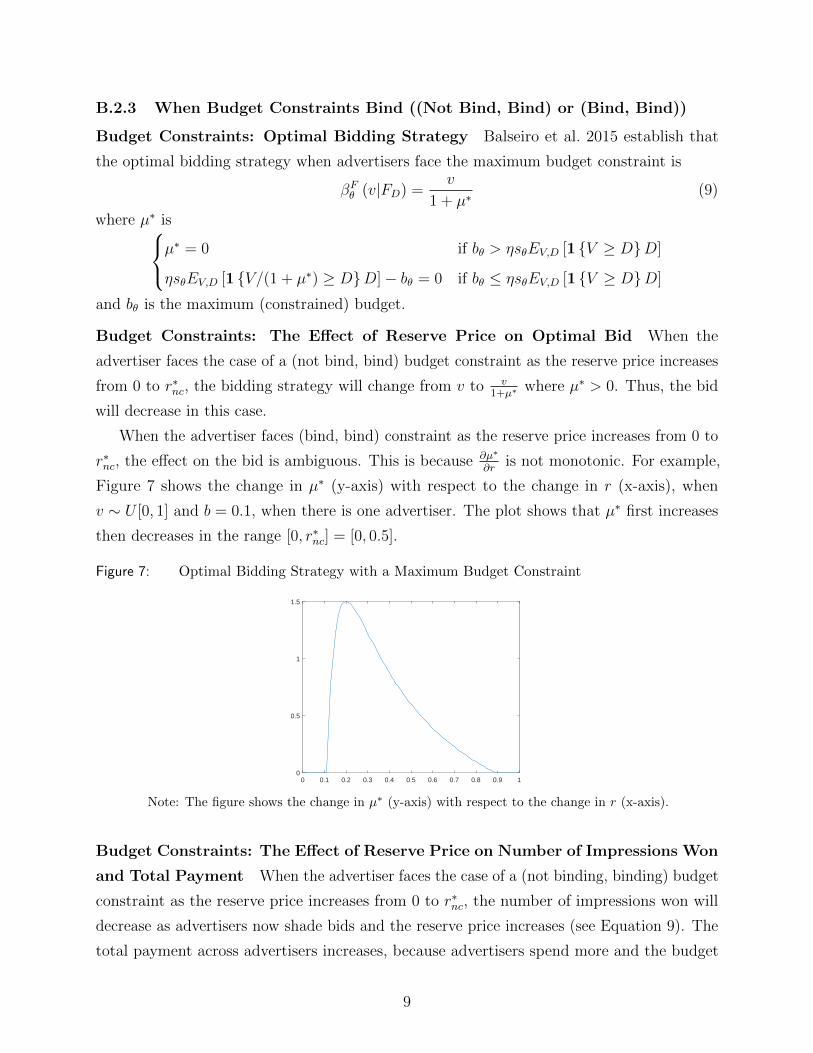
B.2.3 When Budget Constraints Bind ((Not Bind, Bind) or (Bind, Bind))

Budget Constraints: Optimal Bidding Strategy Balseiro et al. 2015 establish that

the optimal bidding strategy when advertisers face the maximum budget constraint is

βFθ (v|FD) =v

1 + µ∗(9)

where µ∗ isµ∗ = 0 if bθ > ηsθEV,D [1 {V ≥ D}D]

ηsθEV,D [1 {V/(1 + µ∗) ≥ D}D]− bθ = 0 if bθ ≤ ηsθEV,D [1 {V ≥ D}D]

and bθ is the maximum (constrained) budget.

Budget Constraints: The Effect of Reserve Price on Optimal Bid When the

advertiser faces the case of a (not bind, bind) budget constraint as the reserve price increases

from 0 to r∗nc, the bidding strategy will change from v to v1+µ∗

where µ∗ > 0. Thus, the bid

will decrease in this case.

When the advertiser faces (bind, bind) constraint as the reserve price increases from 0 to

r∗nc, the effect on the bid is ambiguous. This is because ∂µ∗

∂ris not monotonic. For example,

Figure 7 shows the change in µ∗ (y-axis) with respect to the change in r (x-axis), when

v ∼ U [0, 1] and b = 0.1, when there is one advertiser. The plot shows that µ∗ first increases

then decreases in the range [0, r∗nc] = [0, 0.5].

Figure 7: Optimal Bidding Strategy with a Maximum Budget Constraint

0 0.1 0.2 0.3 0.4 0.5 0.6 0.7 0.8 0.9 10

0.5

1

1.5

Note: The figure shows the change in µ∗ (y-axis) with respect to the change in r (x-axis).

Budget Constraints: The Effect of Reserve Price on Number of Impressions Won

and Total Payment When the advertiser faces the case of a (not binding, binding) budget

constraint as the reserve price increases from 0 to r∗nc, the number of impressions won will

decrease as advertisers now shade bids and the reserve price increases (see Equation 9). The

total payment across advertisers increases, because advertisers spend more and the budget

9

constraint becomes binding.

When the advertiser faces the case of a (binding, binding) budget constraint, the total

payment will stay the same (at the binding budget level), but the effect on the number of

impressions won is ambiguous because bid CPM may or may not increase with respect to the

change in the reserve price.

B.2.4 Other Constraints

When advertisers set pacing options, we expect the results to be similar to the budget

constraint case, as pacing plays a similar role to setting an even budget over a specified time

period. Finally, advertisers’ learning of their own or others’ valuations can either decrease or

increase bid CPM depending on the signals received.48

C Estimation and Policy Simulation

This section overviews the computational algorithms used in estimation and policy simulations.

C.1 Computational Steps in Estimation

The estimation proceeds as follows:

Stage 1 Denoting w = v + µ, FW (w) and FD(d) are non-parametrically estimated as

described in Equations (3) and (4).

Stage 2 Using the optimality condition in Proposition 2, µ∗ is solved for the FMFE using

the following algorithm.

1. Start with an arbitrary vector of multipliers µ. That is µ0θ = µθ, ∀θ ∈ Θ

2. Repeat

(a) Using the estimates(FD(d), FW (w)

)obtained in Stage 1, Nsim simulated values

are drawn from the estimated distributions v ∼ FV = FW (v + µiθ) and d ∼ FD(d)

to construct

h(µθ;µi) =

yθηsθ− 1

Nsim

∑[1 {vsim + µθ ≥ dsim}] (10)

This equation follows from the advertiser’s optimal bidding strategy condition

characterized in Proposition 2. Note that the first term is the advertiser’s minimum

auction winning rate for a given impression and a campaign as computed in Section

4.3, and the second term is the predicted winning rate conditional on µθ.

48 If advertisers have a common value component (Bajari and Hortacsu 2003, Hong and Shum 2002), bids arealso expected to decrease (shade more) when setting the (secret) reserve price, as the seller with the reserveprice is treated as one additional competitor.

10

(b) µi+1θ solves

arg minµθ≥0 h(µθ;µi), ∀θ ∈ Θ

where minimizing h(µθ;µi) over µθ ≥ 0 ensures that the conditions in Proposition

2 are satisfied in equilibrium

(c) Compute the difference 4 = ‖µi+1 − µi‖ and update i = i+ 1

3. Until 4 < ε

C.2 Computational Approach to Computing Optimal Reserves in the Policy

Simulation

This sub-section discusses the numerical approach used to solve for the optimal reserve price.

In order to find the new FMFE under the considered reserve price level, the advertisers’

beliefs on D (which reflects the bids of competing advertisers) need to be updated to ensure

that the advertisers’ new beliefs are consistent with the bidding profile µ(D, r) at the new

reserve price. Thus solving the optimal reserve price with the minimum impression constraint

involves embedding the iterative best-response algorithm. That is, given the recovered Fv,

1. Start with an arbitrary rj for j = 0 (we start with r0 = r∗nc, the optimal reserve when

advertisers bid truthfully)

2. Repeat: r-step

(a) Start with an arbitrary vector of multipliers µ. That is µ0θ = µθ, ∀θ ∈ Θ

(b) Repeat: µ-step

i. Obtain FD(·|µi

)using Equation (3).

ii. µi+1θ solves

arg minµθ≥0 h(µθ;µi), ∀θ ∈ Θ

h(µθ;µi) =

yθηsθ− EV,D [1 {V + µθ ≥ D}]

which finds the bidding strategy profile, µθ, that minimizes the difference

between the minimum winning rate the advertiser aims to attain for a given

impression for a campaign (as computed in sub-section 4.3) and the predicted

winning rate, EV,D [1 {V + µθ ≥ D}], given µθ.

iii. Check the advertiser’s participation constraint

For θ with 0 > EV,D [1 {V + µθ ≥ D} (V −D)], update µi+1θ = µθ where

µθ = argmaxµθ≥0 [0 ≤ ηsθEV,D [1 {V + µθ ≥ D} (V −D)]]

11

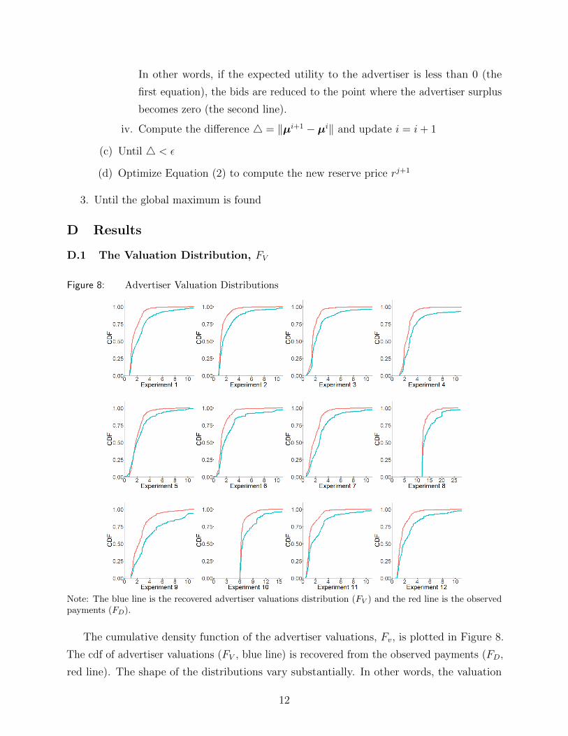
In other words, if the expected utility to the advertiser is less than 0 (the

first equation), the bids are reduced to the point where the advertiser surplus

becomes zero (the second line).

iv. Compute the difference 4 = ‖µi+1 − µi‖ and update i = i+ 1

(c) Until 4 < ε

(d) Optimize Equation (2) to compute the new reserve price rj+1

3. Until the global maximum is found

D Results

D.1 The Valuation Distribution, FV

Figure 8: Advertiser Valuation Distributions

Note: The blue line is the recovered advertiser valuations distribution (FV ) and the red line is the observedpayments (FD).

The cumulative density function of the advertiser valuations, Fv, is plotted in Figure 8.

The cdf of advertiser valuations (FV , blue line) is recovered from the observed payments (FD,

red line). The shape of the distributions vary substantially. In other words, the valuation

12

distributions appear to vary by observables such as (site-ad location-ad size-device-month),

implying that different reserve prices should be set for different auctions.

13