1

MA

ST

ER

FIN

AL

TH

ES

IS

Design of a test bench for the flow ripple determination in positive-displacement hydraulic pumps

Author:

Andrea Gallo

Director /Co-director:

Miquel Torrent Gelmà

/ Pedro Javier Gamez Montero

Degree:

Master in Industrial Engineering

Examination session:

Spring, 2021

Document:

Annexes

2

Contents 1 TEST REPORT .............................................................................................................. 3

TEST CARRIED OUT: .................................................................................................. 3

TEST DATE: ................................................................................................................. 3

TEST PERFORMED BY:............................................................................................... 3

1.1 OBJECTIVE ............................................................................................................ 4

1.2 INSTRUMENTATION .............................................................................................. 4

1.3 PROCEDURES ....................................................................................................... 7

1.4 POSITIVE-DISPLACEMENT PUMP TESTED ......................................................... 9

1.5 TEST CONDITION .................................................................................................10

1.6 RESULTS ...............................................................................................................11

1.6.1 50 bar ..............................................................................................................11

1.6.2 75 bar ..............................................................................................................13

1.6.3 90 bar ..............................................................................................................15

2 LABORATORY PRACTICE ..........................................................................................19

2.1 INTRODUCTION .......................................................................................................19

2.2 OBJECTIVE ...........................................................................................................20

2.3 BASIC FORMULAS ................................................................................................20

2.4 INSTRUMENTATION .............................................................................................21

2.5 POSITIVE-DISPLACEMENT PUMP TESTED ........................................................23

2.6 PROCEDURES ......................................................................................................24

2.7 TEST RESULTS PRESENTATION ........................................................................24

2.8 SHORT QUESTIONS .............................................................................................24

3 MATLAB CODE ........................................................................................................25

3

1 TEST REPORT

TEST CARRIED OUT: Computation of source flow ripple and source impedance of a 10.6 cc/rev external gear pump, following the standard ISO 10767:1-2015

TEST DATE: 12/05/2021

TEST PERFORMED BY: ANDREA GALLO

4

1.1 OBJECTIVE The objectives of this test are:

1. COMPUTATION OF THE SOURCE FLOW RIPPLE 2. COMPUTATION OF THE SOURCE IMPEDANCE

To achieve these objectives, the standard ISO 10767:1-2015 is followed.

1.2 INSTRUMENTATION The instrumentation used during the test is listed in the table below:

Position Instrumentation Brand and type

1 Electric motor MEB BF5 100L 44

2 Positive displacement pump Roquet 1L16DE10R

3 Temperature sensor Elitech TPM10

4 Piezoelectric pressure transducer Kystler 601

5 Charge amplifier Kystler 5039A

6 Piezoresistive pressure transducer Wika MH-3

7 Manometer Wika 232.30

8 Loading valve EDI System SU/M/38

9 Pressure relief valve Roquet SGRA06

10 Steel pipe Protubsa

11 Flexible hoses Voss SP 4

12 Detector IFM IFT200

13 Hydraulic oil Renoil B10

14 Analysing recorder Yogokawa DL716

15 Power supply Mean well S-50-24 Table 1 Test bench's instrumentation

5

Figure 1 Test bench

Figure 2 Test bench's hydraulic scheme

6

Figure 3 Future test bench

7

1.3 PROCEDURES The test is carried out in accordance with the standard ISO 10767:1-2015 [1]. Initially, both the loading valve are left opened for a sufficient time period to avoid a potential presence of air in the circuit. In addition, the digital scope’s sample frequency is set following the Nyquist-Shannon theorem. It is imposed a sampling frequency 2.5 times higher than the tenth harmonic. By knowing the pump’s rotational speed, it is easily computed

(𝑓10 = 10 ∙ 𝑧 ∙ 𝑓𝑠ℎ𝑎𝑓𝑡).

Later with the help of the manometer, the desired mean pressure is obtained by using the first loading valve. In this way the system 1 is achieved. Therefore, the pressure fluctuations are sampled with the digital scope and saved in the floppy disk. After that, the first loading valve is fully opened and the second one is regulated to achieve the same mean pressure. The pressure fluctuations are sampled with the digital scope and saved in the floppy disk. By using the second loading valve, the system 2 is achieved. The difference between the two systems consists in a partial change of the hydraulic circuit which affects the vibration mode of the two systems. That is possible thanks to the use of the extension pipe which is located between the two loading valves. The data are saved in an Excel sheet and converted in the Matlab language. Then, with the help of a Matlab code, the desired characteristic values are computed. The source flow ripple at each harmonic is computed as:

𝑄𝑆𝑖 = 𝑗1

𝑍𝐶

𝑃0𝑖𝑃1𝑖′ − 𝑃0𝑖′𝑃1𝑖

(𝑃0𝑖 − 𝑃0𝑖′)𝑠𝑖𝑛(𝛽𝐿𝑟)

( 1 )

While the source impedance as:

𝑍𝑆𝑖 = 𝑗𝑍𝐶

(𝑃0𝑖 − 𝑃0𝑖′)𝑠𝑖𝑛(𝛽𝐿𝑟)

𝑃1𝑖 − 𝑃1𝑖′(𝑃0𝑖 − 𝑃0𝑖′)𝑐𝑜𝑠(𝛽𝐿𝑟)

( 2 )

Where

• 𝑍𝐶 is the characteristic impedance of the reference pipe

• 𝑃0𝑖 is the 𝑖𝑡ℎ harmonic sampled with the first pressure transducer in the system 1

• 𝑃1𝑖 is the 𝑖𝑡ℎ harmonic sampled with the second pressure transducer in the system 1

• 𝑃0𝑖′ is the 𝑖𝑡ℎ harmonic sampled with the first pressure transducer in the system 2

• 𝑃1𝑖′ is the 𝑖𝑡ℎ harmonic sampled with the second pressure transducer in the system 2

• 𝛽 is the wave propagation coefficient of the reference pipe

• 𝐿𝑟 is the reference pipe’s length Furthermore, is considered the source flow ripple located in the inner part of the discharge line. Therefore, the source flow ripple in the modified model is evaluated as:

𝑄𝑆 ∗= 𝑄𝑆 𝑐𝑜𝑠(𝛽𝑑𝐿𝑑)

( 3 )

Finally, as an example of the usefulness of the previous characteristic values the blocked acoustic pressure is evaluated. Thus, it is supposed that the entry impedance of the hydraulic circuit tends to infinite. Therefore, the theorical pressure ripple are computed as:

|𝑃𝑏𝑖| = |𝑍𝑆𝑖||𝑄𝑆𝑖|

( 4 )

8

Additionally, considering all the ten harmonics taken in consideration, the root mean square of the blocked acoustic pressure is computed as:

|𝑃𝑏𝑅𝑀𝑆| = √|𝑃𝑏1|2+. . . . +|𝑃𝑏10|2

2

( 5 )

9

1.4 POSITIVE-DISPLACEMENT PUMP TESTED The positive-displacement pump tested is the Roquet external gear pump 1L16DE10R, whose volumetric capacity is equal to 10.6 cc/r. It is actioned at 1450 rpm, obtaining a mean flow rate of 15 lpm. In the following table are listed its main characteristics:

Rotation sense 𝑐𝑙𝑜𝑐𝑘𝑤𝑖𝑠𝑒

Driving shaft form 𝑡𝑦𝑝𝑒 𝐸

Port connection 𝑡𝑦𝑝𝑒 𝑅

Max. cont. pressure 275 𝑏𝑎𝑟

Max. rpm 3500 𝑟𝑝𝑚

Number of teeth 12 Table 2 Roquet 1L16DE10R's main characteristics

Figure 4 Roquet 1L16DE10R

10

1.5 TEST CONDITION Three tests are carried out, using three working pressure, 50,75 and 90 bar. During the tests, the fluid’s temperature changes and so also its kinematic viscosity. In table 3 are listed the main fluid’s properties. Working pressure Working temperature Kinematic viscosity

50 bar 25° C 68.24 mm/s2

75 bar 35° C 39.79 mm/s2 90 bar 45° C 30.69 mm/s2

Table 3 Kinematic viscosity at working temperatures

Test information

Positive-displacement pump

Volumetric capacity [cc/rev]

Number of pumping elements

Outlet port dimension [mm]

Mean flow rate [lpm]

Mean working pressure [bar]

Fluid kinematic viscosity [cSt]

Fluid temperature [°C]

Fundamental harmonic [Hz] Table 4 Test general information

11

1.6 RESULTS

1.6.1 50 bar The first test is carried out at a mean pressure of 50 bar and at a temperature equal to 25° C. The values of the source flow ripple of the first ten harmonics, computed using the Norton model are plotted in figure 5:

Figure 5 Module of the flow ripple computed with the Norton model

The experimental results present a peak at the fundamental harmonic equal to 0.9 lpm, while the following harmonics see a decrease of the module of more than three times. Thus, the hydraulic noise found for this working condition is found to be, as expected, in the first three harmonics. The results evaluated considering the source flow ripple located exactly at the outlet port of the pump are confirmed in terms of trend of the experimental points also considering its real position (“modified model”), but differs in terms of amplitude, obtaining a peak value equal to 1.08 lpm and lower values in the following harmonics. Thus, it is possible to state that the pump at this condition has a good response in term of flow ripple, showing only one important peak.

Figure 6 Module of flow ripple computed with the modified model

12

Moreover, the trend of the flow fluctuation is also plotted in time domain. At each cycle, there is one main fluctuation, accompanied by a minor one. The latter ones can be attributed to the contribution of the second and the third harmonic, while the fundamental harmonic generates the main peak. Moreover, compared to the theoretical curve, the experimental results are very reliable, having the same trend and the same amplitude.

Figure 7 Comparison between the experimental and theorical time history wave form of pressure ripple

In figure 8 the module of the source impedance is plotted:

Figure 8 Module of the source impedance

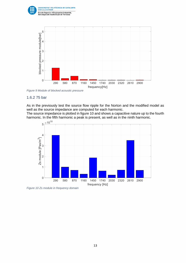
The plot shows a not homogenous trend of the source impedance, which finds three main peaks at the third, the fifth and the ninth harmonic, the latter is the most important. These results show that the impedance of the pump has not a capacitive nature. Additionally, the blocked acoustic pressure is computed. Consequently, in case of an infinite entry impedance 𝑍𝑒 of the hydraulic circuit, a decreasing trend of the pressure is computed, which shows a peak of approximately of 1.3 bar located at 290 Hz, while at the other frequencies the module is one order of magnitude lower. Moreover, the overall root mean square value is equal to 0.96 bar.

13

Figure 9 Module of blocked acoustic pressure

1.6.2 75 bar As in the previously test the source flow ripple for the Norton and the modified model as well as the source impedance are computed for each harmonic. The source impedance is plotted in figure 10 and shows a capacitive nature up to the fourth harmonic. In the fifth harmonic a peak is present, as well as in the ninth harmonic.

Figure 10 Zs module in frequency domain

14

Figure 11 Module of flow ripple in Norton model representation in time domain

The experimental results remark the expected behaviour of external gear pumps, and thus, having a peak in the first harmonic, which at 75 bar is almost equal to 0.8 lpm, and lower contributions, which occur in the successive harmonics, whose absolute values are three times lower respect the one corresponding to the fundamental harmonic. To have a more realistic representation of the source flow ripple, it is preferable to compute it with the modified model and so taking in account also the fluctuations which occurs in the inner part of the discharge line.

Figure 12 Module of flow ripple in modified model representation in time domain

As it is possible to see, the main difference between the two models is found in the second, the third and the fourth harmonic, where the module of the flow fluctuations decreases, but generally speaking, the two models follow the same decreasing trend, remarking so the good design of the hydraulic pump, having found only a significative peak in the first harmonic. Moreover, figure 13 compares the time history wave form computed experimentally and through the theorical model. As well as in the previous test, the experimental results are validated. In fact, the two curves have the same trend, even if the experimental one does not follow perfectly the theorical inverted parabola, presenting two additional peaks, that can be attributed to range of frequencies between 580 Hz and 1160 Hz.

15

Figure 13 Flow fluctuations in time domain

Furthermore, the blocked acoustic pressure is shown in figure 14.

Figure 14 Blocked acoustic pressure in frequency domain

The maximum peak is located at the fundamental harmonic where is found a value of more than 5 bar, while the other harmonics show irrelevant contributions. The overall root mean square value is equal to 3.77 bar.

1.6.3 90 bar In the last test a mean working pressure of 90 bar is used, while the fluid temperature is equal to 45°C. The results in term of source impedance remark the ones computed at 50 bar. As the figure 15 shows, the pump impedance exhibits two peaks at 1450 Hz and at 2610 Hz. Consequently, if up to 1KHz it has a capacitive nature, from the fourth harmonic the inertia of the working fluid cannot be neglected, showing an inductance nature.

16

Figure 15 Module of source impedance in harmonic spectra

Regarding the flow ripple evaluated using the Norton model, as in the test carried out at 75 bar, it exhibits a peak of almost 0.8 lpm at 290 Hz, while the second harmonic shows a halved value respect the fundamental one. Furthermore, also at 870 Hz an important contribution is found, exhibiting a wider range of hydraulic noise respect the test at 50 bar.

Figure 16 Module of flow ripple source (Norton model)

When the modified model is used, a better behaviour of the pump is exhibited. Even if the main contribution is almost unchanged (0.7 lpm respect to 0.8 lpm), the following harmonics show a large decrease, having values with one order of magnitude lower respect the fundamental harmonic.

17

Figure 17 Module of flow ripple source (modified model)

Furthermore, the fluctuations in time domain reflect the ones found at 50 bar, with the main peak belonging to the first harmonic and very small deflections respect to the theorical inverted parabola. The only difference with the mathematical model consists in the range of amplitude where the two curves lie, between 20 and -20⋅10-6 m3/s the model and between

10 and -15⋅10-6 m3/s the empirical results.

Figure 18 Flow ripple fluctuations in time domain

Moreover, respect to the other tests, the blocked acoustic pressure presents lower values in both the fundamental and the other harmonics. In addition, the overall root mean square value is equal to 0.57 bar.

18

Figure 19 Blocked acoustic pressure

19

2 LABORATORY PRACTICE

2.1 INTRODUCTION Depending on their working principles hydraulic pumps can be classified in two main categories, rotodynamic pump, where a rotary element called impeller imparts energy to the fluid and positive-displacement pump. The first class is used when the main goals are working with high flow rates and low pressures, while positive-displacement pumps are applied when is required to work with high pressures, and low flow rates. The latter type of pumps can additionally be divided in different sub-categories and the most important are rotatory and reciprocating pumps. Their common characteristic is that under ideal condition the flow rate generated depends only on the rotational speed and on the pump derived capacity (𝑄𝑡ℎ = 𝑛 ∙ 𝑐𝑣). Where the latter characteristic is defined as the volume of fluid delivered at each working cycle. Consequently, compared to turbomachinery, the flow rate is not affected by the working pressure. The main disadvantage of positive displacement pumps is related to the delivered flow rate since it fluctuates over time and consequently causes vibrations and noises in the hydraulic circuit. The flow ripple is caused by their working principle. During their working cycle, the pumping elements (such as pistons, gear teeth or vanes), deliver a volume of fluid that in time can be described as half sine wave. Summing altogether the different flow contributions is found a variable trend over time.

Figure 20 Instantaneous flow rate of an axial piston pump

Moreover, the flow rate irregularity is defined as:

𝜎 =Qmax − Qmin

Qmean

20

2.2 OBJECTIVE The objectives of this practice are:

3. COMPUTATION OF THE SOURCE FLOW RIPPLE 4. COMPUTATION OF THE SOURCE IMPEDANCE

To achieve these objectives, the standard ISO 10767:1-2015 is followed.

2.3 BASIC FORMULAS

• SOURCE FLOW RIPPLE (NORTON MODEL):

𝑄𝑆𝑖 = 𝑗1

𝑍𝐶

𝑃0𝑖𝑃1𝑖′ − 𝑃0𝑖′𝑃1𝑖

(𝑃0𝑖 − 𝑃0𝑖′)𝑠𝑖𝑛(𝛽𝐿𝑟)

( 1 )

• SOURCE IMPEDANCE:

𝑍𝑆𝑖 = 𝑗𝑍𝐶

(𝑃0𝑖 − 𝑃0𝑖′)𝑠𝑖𝑛(𝛽𝐿𝑟)

𝑃1𝑖 − 𝑃1𝑖′(𝑃0𝑖 − 𝑃0𝑖′)𝑐𝑜𝑠(𝛽𝐿𝑟)

( 2 )

• SOURCE FLOW RIPPLE (MODIFIED MODEL) 𝑄𝑆 ∗= 𝑄𝑆 𝑐𝑜𝑠(𝛽𝑑𝐿𝑑)

( 3 )

• BLOCKED ACOUSTIC PRESSURE |𝑃𝑏𝑖| = |𝑍𝑆𝑖||𝑄𝑆𝑖|

( 4 )

• CIRCUIT’S CHARACTERISTIC IMPEDANCE

𝑍𝐶 =𝜌𝑐ξ(ω)

𝜋𝑟𝑂2

( 5 )

• UNSTEADY VISCOUS FRICTION COEFFICIENT

ξ(ω) = 1 + √𝑣

2𝑟02𝜔

− 𝑗 (√𝑣

2𝑟02𝜔

+𝑣

2𝑟02𝜔

)

( 6 )

• WAVE PROPAGATION COEFFICIENT

𝛽 =ξ(ω) ∙ ω

𝑐

( 7 )

Where, 𝐿𝑟 is the reference pipe’s length 𝑐 is the speed of sound

21

2.4 INSTRUMENTATION The instrumentation used during the test is listed in the table below:

Position Instrumentation Brand and type

1 Electric motor MEB BF5 100L 44

2 Positive displacement pump Roquet 1L16DE10R

3 Temperature sensor Elitech TPM10

4 Piezoelectric pressure transducer Kystler 601

5 Charge amplifier Kystler 5039A

6 Piezoresistive pressure transducer Wika MH-3

7 Manometer Wika 232.30

8 Loading valve EDI System SU/M/38

9 Pressure relief valve Roquet SGRA06

10 Steel pipe Protubsa

11 Flexible hoses Voss SP 4

12 Detector IFM IFT200

13 Hydraulic oil Renoil B10

14 Analysing recorder Yogokawa DL716

15 Power supply Mean well S-50-24 Table 5 Test bench's instrumentation

22

Figure 21 Test bench

Figure 22 Test bench's hydraulic scheme

23

2.5 POSITIVE-DISPLACEMENT PUMP TESTED The positive-displacement pump tested is the Roquet external gear pump 1L16DE10R, whose volumetric capacity is equal to 10.6 cc/r. In the following table are listed its main characteristics:

Rotation sense 𝑐𝑙𝑜𝑐𝑘𝑤𝑖𝑠𝑒

Driving shaft form 𝑡𝑦𝑝𝑒 𝐸

Port connection 𝑡𝑦𝑝𝑒 𝑅

Max. cont. pressure 275 𝑏𝑎𝑟

Max. rpm 3500 𝑟𝑝𝑚

Number of teeth 12 Table 6 Roquet 1L16DE10R's main characteristics

Figure 23 Roquet 1L16DE10R

24

2.6 PROCEDURES The procedures will be the following ones:

1. Start the engine and the electronic devices. 2. Leave the two loading valves open for a sufficient period of time. 3. Regulate the first loading valve to achieve the required mean pressure. 4. Sample the pressure fluctuations with the digital scope and save the data. 5. Leave the first loading valve open and regulate the second loading valve to

achieve the same mean pressure. 6. Sample the pressure fluctuations and save the data. 7. Compute the required values.

The test must be carried out under the supervision of the laboratory staff.

2.7 TEST RESULTS PRESENTATION You have to present a laboratory report which includes:

1. Table which includes the test conditions and data. 2. DFT graphic for all the four pressure signals. 3. Graphic QS-Frequency for both the Norton and modified model. 4. Graphic ZS-Frequency. 5. Graphic PB-Frequency and its RMS value.

The graphic should be as the one shown in figure 5.

Figure 24 Source flow ripple module

2.8 SHORT QUESTIONS

1. Compute the flow rate if the rotational speed is equal to 2000 rpm. 2. Which is the pumping frequency if the number of teeth is equal to 10? 3. According to the Nyquist-Shannon theorem which is the most adequate sampling

frequency to choose in the digital scope?

25

3 MATLAB CODE clear all clc T=35; %temperature f=([290;580;870;1160;1450;1740;2030;2320;2610;2900]); % theorical frequencies fs=10000; %sampling frequency %% fluid charactheristics pho=876; %density l=0.15; %length v=30.69; %viscosity c=1280.82366; %speed of sound r1=8; %mm r=8/1000; %internal radius w=zeros(1,10); zita=zeros(1,10); b=zeros(1,10); jzcd=zeros(1,10); jzc=zeros(1,10); rez=zeros(1,10); imz=zeros(1,10); for k=1:10 w(k)=2*pi*290*k; end for k=1:10 rez(k)=(1+(sqrt((v/(2*r1^2.*w(k)))))); imz(k)=-(sqrt((v/(2*r1^2.*w(k))))+(v/(r1^2.*w(k)))); zita(k)=complex(rez(k),imz(k)); b(k)=(zita(k).*w(k))/c; zc(k)=((pho*c).*zita(k))/(pi*r^2); jzcd(k)=1i/zc(k); jzc(k)=1i*zc(k); end %% now we start computing P0 values Y1=xlsread('1st1st.xlsx'); Y1=Y1.*(3.125*10^6); %get Pa N=length(Y1); time=linspace(0,1,N); figure (90) plot(time, Y1,'r','LineWidth',1.5) set(gca,'FontSize',24) xlabel('time [s]') ylabel('pressure [Pa]'); xlim([0,0.015]) minn1=min(Y1); maxx1=max(Y1); delta1=(maxx1-minn1)*10^-5; %bar value means=mean(Y1); y1=2*fft(Y1,N)/N; %FFT xx=linspace(0,fs,N)';

26

figure (1) stem(xx,abs(y1),'r','LineWidth', 4) xlim([5,2950]) ylim([0,10e4]) xlabel('frequency [Hertz]') ylabel('pressure [Pa]'); set(gca,'FontSize',24) legend('1st transducer 1st loading valve') grid on %% 2nd trans 1st valve Y2=xlsread('2nd1st.xlsx'); Y2=Y2.*(3.125*10^6); y2=2*fft(Y2,N)/N; %FFT figure (2) stem(xx,abs(y2),'r','LineWidth', 4) set(gca,'FontSize',24) xlim([5,2950]) ylim([0,10e4]) xlabel('frequency [Hertz]') ylabel('pressure [Pa]'); legend('2nd transducer 1st loading valve') grid on minn2=min(Y2); maxx2=max(Y2); delta2=(maxx2-minn2)*10^-5; %bar value %% 1st tran 2nd valve Y3=xlsread('1st2nd.xlsx'); Y3=Y3.*(3.125*10^6); y3=2*fft(Y3,N)/N; %FFT figure (3) stem(xx,abs(y3),'LineWidth', 4) xlim([5,2950]) ylim([0,10e4]) set(gca,'FontSize',24) xlabel('frequency [Hertz]') ylabel('pressure [Pa]'); legend('1st transducer 2nd loading valve') grid on minn3=min(Y3); maxx3=max(Y3); delta3=(maxx3-minn3)*10^-5; %bar value %% 2nd 2nd Y4=xlsread('2nd2nd.xlsx'); Y4=Y4.*(3.125*10^6); y4=2*fft(Y4,N)/N; %FFT figure (4) stem(xx,abs(y4),'LineWidth', 4) set(gca,'FontSize',24) xlim([5,2950]) ylim([0,10e4]) xlabel('frequency [Hertz]') ylabel('pressure [Pa]');

27

legend('2nd transducer 2nd loading valve') grid on minn4=min(Y4); maxx4=max(Y4); delta4=(maxx4-minn4)*10^-5; %bar value %% computation Pressure parameters zz=0; fre=zeros(1,10); rr=0; index1=0; p0=zeros(1,10); % vector of complex pression value0=zeros(1,10); pv=complex(0,0); %var for i=270:290 if abs(y1(i))>rr index1=i; rr=abs(y1(i)); end end for i=1:10 fre(i)=index1*i; end for i=1:10 for k=(fre(i)-15):(fre(i)+15) if abs(y1(k))>zz zz=abs(y1(k)); pv=y1(k); value0(i)=k; else zz=zz; end p0(i)=pv; end zz=0; end zz=0; pv=complex(0,0); %% p1 fre=zeros(1,10); rr=0; value1=zeros(1,10); index2=0; p1=zeros(1,10); % vector of complex pressure for i=270:290 if abs(y2(i))>rr index2=i; rr=abs(y2(i)); end end for i=1:10 fre(i)=index2*i; end for i=1:10

28

for k=(fre(i)-15):(fre(i)+15) if abs(y2(k))>zz zz=abs(y2(k)); pv=y2(k); value1(i)=k; else zz=zz; end p1(i)=pv; end zz=0; % end of each loop end zz=0; pv=complex(0,0); %% p0' zz=0; fre=zeros(1,10); value2=zeros(1,10); rr=0; index3=0; p00=zeros(1,10); % vector of complex pressure pv=complex(0,0); %var for i=270:290 if abs(y3(i))>rr index3=i; rr=abs(y3(i)); end end for i=1:10 fre(i)=index3*i; end for i=1:10 for k=(fre(i)-15):(fre(i)+15) if abs(y3(k))>zz zz=abs(y3(k)); pv=y3(k); value2(i)=k; else zz=zz; end p00(i)=pv; end zz=0; % end of each loop end zz=0; pv=complex(0,0); %% p1' zz=0; fre=zeros(1,10); value3=zeros(1,10); rr=0; index4=0; p01=zeros(1,10); % vector of complex pressure pv=complex(0,0); %var

29

for i=270:290 if abs(y4(i))>rr index4=i; rr=abs(y4(i)); end end for i=1:10 fre(i)=index4*i; end for i=1:10 for k=(fre(i)-15):(fre(i)+15) if abs(y4(k))>zz zz=abs(y4(k)); pv=y4(k); value3(i)=k; else zz=zz; end p01(i)=pv; end zz=0; % end of each loop end %% Qs and Zs qs=zeros(1,10); zs=zeros(1,10); for k=1:10 qs(k)=jzcd(k).*(((p0(k)*p01(k))-(p00(k)*p1(k)))/((p0(k)-p00(k))*sin(b(k)*l))); end for k=1:10 zs(k)=jzc(k)*(((p0(k)-p00(k))*sin(b(k)*l))/((p1(k)-p01(k))-((p0(k)-p00(k))*cos(b(k)*l)))); end figure (5) bar(f,abs(qs)*10^6,'r','LineWidth',1.5); xlabel('frequency [Hz]') ylabel('Qs module [10e-6 m^3/s]') set(gca,'FontSize',24) ylim([0,20]) grid on figure (6) bar(f,abs(zs),'b','LineWidth', 1.5); ylim([0,0.5*10^11]) xlabel('frequency [Hz]') ylabel('Zs module [Pas/m^3]') set(gca,'FontSize',24) grid on %% q(time) phaseqs=zeros(1,10); for k=1:10 phaseqs(k)=angle(qs(k))*180/pi; end phasezs=zeros(1,10); for k=1:10 phasezs(k)=angle(zs(k))*180/pi;

30

end %% QS* qss=zeros(1,10); for k=1:10 qss(k)=((zs(k)./(sqrt(zs(k).^2-zc(k).^2))).*qs(k)); end figure (7) bar(f,abs(qss)*10^6,'r','LineWidth', 1.5) xlabel('frequency [Hz]') ylabel('Qs* module [10e-6 m^3/s]') ylim([0,20]) set(gca,'FontSize',24) grid on phaseqss=zeros(1,10); for k=1:10 phaseqss(k)=angle(qss(k))*180/pi; end %% q(t) in time tout=4/290; x=linspace(0,tout,10000); y=linspace(0,0,10000); for t=1:10000 for k=1:10 y(t)=y(t)+(abs(qss(k))*10^6*(cos((2*pi*f(k)*x(t))+phaseqss(k)))); end end figure (8) plot(x,y,'r','LineWidth', 2) set(gca,'FontSize',24) xlabel('time[s]') ylabel('q(t)*[10e-6 m^3/s]') ylim([-25,+25]) hold on kk=x(1566); %starting of the cycle qmax=16; fii=linspace(-pi/12,pi/12,1000)'; k=(543030.59*10^-6)*60; yyy=-248.0573+2.1093+(qmax-k.*(fii.^2))/60*10^3; xxx=linspace(kk,1/290+kk,1000)'; xxx1=linspace(1/290+kk,2/290+kk,1000)'; xxx2=linspace(2/290+kk,3/290+kk,1000)'; plot(xxx,yyy,'b','LineWidth', 2) ylim([-25,+25]) hold on plot(xxx1,yyy,'b','LineWidth', 2) ylim([-25,+25]) hold on plot(xxx2,yyy,'b','LineWidth',2) ylim([-25,+25]) grid on legend('experimental flow ripple','mathematical model')

31

%% blocked pressure pb=zeros(1,10); for k=1:10 pb(k)=zs(k)*qs(k); end figure (9) bar(f,abs(pb)*10^-5,'r','LineWidth', 1.5); set(gca,'FontSize',24) xlabel('frequency[Hz]') ylabel('blocked pressure module[bar]') ylim([0,5.5]) grid on %% lumped parameter model c1=0; for k=1:10 c1=c1+imag(zs(k)*f(k)); end c1=c1/10; zsml=zeros(1,10); for k=1:10 zsml(k)=c1/complex(0,f(k)); end %% lumped c11=0; for k=1:10 c11=c11+abs(imag(zs(k)*f(k))); end c11=c11/10; zsmla=zeros(1,10); for k=1:10 zsmla(k)=c11/complex(0,f(k)); end figure (10) bar(f,phaseqs,'r','LineWidth', 1.5) set(gca,'FontSize',24) xlabel('frequency [Hz]') ylabel('qs phase [deg]') figure (11) bar(f,phasezs,'r','LineWidth', 1.5) set(gca,'FontSize',24) xlabel('frequency [Hz]') ylabel('zs phase [deg]') grid on %% qs and zs verification qov=zeros(1,10); p1v=zeros(1,10); for k=1:10 qov(k)=qs(k)-(p0(k)/zs(k)); end for k=1:10 p1v(k)=(cos(b(k)*l)*p0(k))-(jzc(k)*sin(b(k)*l).*qov(k)); end

32

error=zeros(1,10); for k=1:10 error(k)=(abs(p1(k))-abs(p1v(k)))/abs(p1(k))*100; end figure (12) pression1=[p1;p1v]'; bar(f,abs(pression1),'LineWidth',1.5) set(gca,'FontSize',24) legend('p1 computed','p1 experimental') grid on %% distrubeted parameter c2=pi/(2*2030) c1=(zs(3)+zs(4))/2 bb=0.7 %correction factor alfa=zeros(1,10); sigma1=zeros(1,10); sigma2=zeros(1,10); j=complex(0,1); t1=0; t2=0; s11=0; s12=0; s21=0; s22=0; for k=1:100 for i=1:10 alfa(i)=(j*zs(i)*sin(f(i)*c2))-(c1*cos(f(i)*c2)); sigma1(i)=-cos(f(i)*c2); sigma2(i)=(j*zs(i)*f(i)*cos(f(i)*c2))+(f(i)*c1*sin(f(i)*c2)); t1=t1+real(alfa(i)*conj(sigma1(i))); t2=t2+real(alfa(i)*conj(sigma2(i))); s11=s11+real(conj(sigma1(i))*sigma1(i)); s12=s12+real(conj(sigma1(i))*sigma2(i)); s21=s21+real(conj(sigma2(i))*sigma1(i)); s22=s22+real(conj(sigma2(i))*sigma2(i)); end deltac1=((t2*s12)-(t1*s22))/((s11*s22)-(s21*s12)); deltac2=((t1*s21)-(t2*s11))/((s11*s22)-(s21*s12)); if abs(deltac1)<=(c1*10^-3) | abs(deltac2)<=(c2*10^-3) c1=c1; c2=c2; k=100 else c1=c1+(bb*deltac1); c2=c2+(bb*deltac2); end end zsmd=zeros(1,10); for i=1:10 zsmd(i)=c1/(j*tan(c2*f(i))); end

33

figure (13) loglog(f,abs(zsmd),'b',f,abs(zs),'x','LineWidth',2) ylim([0,3.5*10^11]) hold on loglog(f,abs(zsml),'r','LineWidth', 2) ylim([0,3.5*10^11]) legend('distributed parameter','experimental','lumped parameter') set(gca,'FontSize',24) xlabel('frequency [Hz]') ylabel('Zs module [Pas/m^3]') ylim([0,3.5*10^11]) grid on %% pb rms pbrms=0; for i=1:10 pbrms=pbrms+abs(pb(i))^2; end pbrms=sqrt(pbrms/2); pbrms*10^-5;