Dispersion in Options Traders’ Expectations and StockReturn Predictability∗

Panayiotis C. Andreou†,‡ Anastasios Kagkadis§ Paulo Maio¶

Dennis Philip‡

April 2015

∗We would like to thank Yakov Amihud, Turan Bali, Suleyman Basak, Stephen Brown, FrankieChau, George Constantinides, Damian Damianov, Gregory Eaton, Bruce Grundy, Hui Guo, MadhuKalimipalli, Neil Kellard, Eirini Konstantinidi, Robert Korajczyk, Alexandros Kostakis, YuehaoLin, Hao Luo, Hong Luo, James Mitchell, Bradley Paye, Ilaria Piatti, David Rapach, Esther Ruiz,Fabio Trojani, Masahiro Watanabe, Hao Zhou and seminar and conference participants at AthensUniversity of Economics and Business, Nottingham University Business School, MFS Symposium,Arne Ryde 2014 Workshop (Lund University), EFMA 2014 Meeting, Modelling Macroeconomic andFinancial Time Series Conference (Loughborough University), NFA 2014 Conference, FMA 2014Meeting, Paris 2014 Finance Meeting and MFA 2015 Meeting for helpful comments and suggestions.We are also grateful to Kenneth French, Amit Goyal, Martin Lettau, Robert Shiller and Hao Zhoufor making data available on their websites. A previous version of this paper was circulated underthe title “Stock Market Ambiguity and the Equity Premium”. Any remaining errors are our own.†Department of Commerce, Finance and Shipping, Cyprus University of Technology, 140, Ayiou

Andreou Street, 3603 Lemesos, Cyprus; Email: benz@pandreou.com‡Durham University Business School, Mill Hill Lane, Durham DH1 3LB, UK; Email: den-

nis.philip@durham.ac.uk§Department of Accounting and Finance, Lancaster University Management School, Lancaster

LA1 4YX, UK; Email: a.kagkadis@lancaster.ac.uk¶Hanken School of Economics, P.O. Box 479, 00101 Helsinki, Finland; Email: paulof-

maio@gmail.com

Abstract

We propose a measure of dispersion in options traders’ expectations about future stock re-turns by using the dispersion in trading volume across strike prices. An increased dispersionin expectations forecasts lower excess market returns at both short and long horizons, whileits out-of-sample predictability is both statistically and economically significant. The sug-gested dispersion measure is highly correlated with the dispersion in analysts’ forecasts butit consistently exhibits a stronger predictive ability. Further, it exhibits additional predic-tive power when combined with the variance risk premium, showing that the two variablescapture different aspects of the variation in returns.

JEL Classification: G10, G11, G12, D81

Keywords: Dispersion in beliefs; Disagreement; Ambiguity; Predictability of stock returns;Equity premium; Trading volume dispersion; Out-of-sample predictability; Economic signif-icance

1 Introduction

A growing body of studies has shown that various measures of dispersion in expectations

can provide significant stock return predictability at both an individual and an aggregate

level. There are two main strands in this literature. A first stream of papers assumes a het-

erogeneous investors framework and uses dispersion to proxy for the level of disagreement

among market participants (e.g. Diether, Malloy and Scherbina, 2002; Yu, 2011; Jiang and

Sun, 2014). Disagreement can affect asset returns either due to the existence of trading fric-

tions in the market or by inducing investors to engage into risk-sharing acts that affect asset

prices in equilibrium. A second strand of the literature assumes a homogeneous investors

framework and uses dispersion to proxy for the level of ambiguity perceived by investors (e.g.

Anderson, Ghysels and Juergens, 2009; Drechsler, 2013). Ambiguity can affect asset returns

due to the fact that naturally investors exhibit aversion to events with unknown probability

distributions.

In this paper, we explore the information content of the dispersion in options traders’

expectations for future market excess returns. To this end, we construct a novel dispersion

in expectations measure that is represented by the dispersion in the volume-weighted strike

prices of equity index option contracts. In light of this, a high dispersion of trading volume

across strike prices is associated with a high dispersion in beliefs in the options market and

vice versa.

The suggested measure is motivated by a simple theoretical framework within which op-

tions end-users engage in trading activities with market makers driven by their expectations

about the future price of the underlying asset. We posit that in such a case the expected

returns of the end-users are naturally reflected in the strike prices at which the options trad-

ing strategies are implemented. For example, the obvious choices for an optimistic investor

would be either to buy a call option or sell a put option. In the first case, an increase in the

asset price increases the investor’s final payoff, while in the second case it ensures that the

option will not be exercised at maturity and the investor will secure the option premium. In

1

addition, the more optimistic the investor, the higher the strike price she will choose. This

is because an out-of-the-money (OTM) option has a lower premium and exhibits a higher

lambda1 than an in-the-money (ITM) option. Therefore, a call buyer (put seller) will be

inclined to select a strike price that is as low as possible in order to ensure that the call will

be exercised (the put will expire worthless), but is as high as possible in order to benefit

from the higher lambda (higher premium). Therefore, due to this trade-off the selected strike

price will reflect the investor’s expectation about the future underlying asset price, in the

sense that a more positive expectation will result in a trade at a more OTM call or a more

ITM put option.2

Furthermore, the put-call parity suggests that an optimistic investor can replicate the

payoff from buying a call option (selling a put option) by borrowing at the risk-free rate and

buying a put option and the underlying asset (selling a call option and buying the underlying

asset). Therefore, by inverting the argument above, it is easy to see that a more positive

expectation will be associated with a trade at a more ITM put or a more OTM call. The

above arguments can be easily reversed and hold for the case of a pessimistic investor as well.

Moreover, the arguments can be extended to the case of more complicated trading strategies

(e.g. call or put spreads and backspreads), since such strategies can be decomposed into a

series of simpler ones. As a result, the overall expectation implied by such a strategy can be

seen as an aggregation of the different expectations implied by the simpler ones. The above

discussion illustrates that any option trade can be theoretically linked to a specific expected

return through the strike price at which it was implemented.

Compared to prior studies, which develop dispersion in beliefs measures based on ana-

lysts’ forecasts or mutual fund and individual investor portfolio holdings,3 the dispersion in

1The lambda (or leverage) of an option is the elasticity of the option price to changes in the underlyingasset price. It is defined as the ratio of the percentage change in the option price to the percentage changein the underlying asset price.

2In practice it is possible that other factors such as market liquidity or limits to arbitrage may play someadditional role in the options positions taken. To the extent, however, that options trading is mainly drivenby traders’ expected asset returns, the framework described here is reasonable.

3Diether, Malloy and Scherbina (2002); Park (2005); Anderson, Ghysels and Juergens (2005, 2009); Yu(2011) and Buraschi, Trojani and Vedolin (2014), among others, utilize the dispersion in analysts’ forecasts,

2

options traders’ expectations exhibits several advantageous characteristics. First, it stems

from all the trades that take place in a highly liquid options market, thus capturing all the

expectations that are considered probable enough to trigger a trade.4 In contrast, analysts’

forecasts constitute only a limited set of opinions,5 and have been found to be affected by

agency issues between firms and investment banks and to be prone to analysts’ behavioral

biases (Dechow, Hutton and Sloan, 2000; Daniel, Hirshleifer and Teoh, 2002; Cen, Hilary

and Wei, 2013). Second, it is directly related to expected returns, while analysts’ predictions

refer to alternative economic indicators such as corporate earnings and hence supplementary

modeling assumptions are needed to derive expectations about returns. Third, unlike dis-

persion measures constructed from analysts’ forecasts or mutual fund holdings data, it can

be estimated on an even higher frequency than monthly or quarterly, thus providing a much

more realistic picture of the evolution of dispersion in expectations across time. Moreover,

the Chicago Board Options Exchange (CBOE) provides freely on its website the intraday

trading activity of option contracts, thus making it easy for investors to use the dispersion in

options traders’ beliefs measure for investment decisions. Fourth, our measure can equally

accommodate optimistic and pessimistic beliefs since it is hardly influenced by the short-

sale constraints present in the equity market that affect both individual and institutional

investor portfolio holdings.6 Finally, it can explicitly distinguish between different levels of

positive and negative expectations, while this is not straightforward in the case of dispersion

measures derived from investors’ positions in the equity market.

Our results establish a significant and robust negative relationship between the dispersion

in options traders’ beliefs and future market returns. In particular, an in-sample regression

while Chen, Hong and Stein (2002); Goetzmann and Massa (2005) and Jiang and Sun (2014) create dispersionmeasures from mutual fund and individual investor portfolio holdings.

4The available range of strike prices for index options is determined by the underlying index fluctuationsand the customer requests. CBOE Rule 24.9.04 specifies that typically strike prices for index options shouldbe within 30% of the current index value, but even more extreme strike prices are permitted provided thereis demonstrated customer demand.

5For example, the average number of forecasters in Anderson, Ghysels and Juergens (2009) is 36.6Almazan, Brown, Carlson and Chapman (2004) provide evidence showing that approximately only 3%

of all mutual funds implement short-selling.

3

analysis shows that at the 1-month horizon, the suggested measure of dispersion in expecta-

tions is a strong predictor of future excess market returns under various model specifications

(univariate and multivariate). Moreover, it outperforms in terms of predictive power all other

predictors examined in prior literature apart from the variance risk premium (VRP), which

explains a higher proportion of the variation in future returns. In addition, it offers addi-

tional predictability when combined with VRP in the same forecasting model, thus showing

that the two variables have different information content and can be used complementarily

for predicting future market returns.7 The results from long-horizon regression analysis show

that our dispersion in beliefs measure remains significant at all horizons, and for horizons of

12 and 24 months ahead exhibits an adjusted R2 higher than 10%, outperforming the major-

ity of the alternative predictors. It is also important to note that while it is highly correlated

(about 60%) with the dispersion in analysts’ forecasts measure (AFD) of Yu (2011), its long-

horizon predictive ability is clearly superior to that of the dispersion in analysts’ forecasts.

The above results are noteworthy because unlike AFD and the majority of the other pre-

dictors, the dispersion in options traders’ expectations exhibits a relatively low persistence

(about 0.50) hence alleviating potential concerns regarding spurious predictability.

The results of out-of-sample predictive analysis reveal that the dispersion of options

traders’ beliefs has significantly higher forecasting power than the historical mean and it

outperforms all other predictive variables (including the dispersion in analysts’ forecasts)

apart from VRP. Following Campbell and Thompson (2008), imposing a constraint of posi-

tive forecasted equity premia leads to further improvement of the out-of-sample predictability

of dispersion in beliefs for the excess market return.

The results are also economically significant since an active trading strategy based on

7Compared to the VRP, which has emerged as the primary option-implied return predictor, the dispersionin options traders’ expectations is conceptually different. First, it is not extracted from option prices andtherefore it is not derived from the risk-neutral distribution. Second, while the level of trading volumecould potentially have an effect on option prices and subsequently on VRP in accordance with the limitsto arbitrage hypothesis (Bollen and Whaley, 2004), high trading volume is not necessarily associated withhigh dispersion across different moneyness categories. Therefore, the market forces that influence VRP donot have an apparent effect on the dispersion in options trading volume across strike prices. In fact, theempirical analysis suggests that the correlation between the two measures is close to zero.

4

the out-of-sample predictive power of the proposed dispersion in expectations measure offers

increased utility to a mean-variance investor that would otherwise follow a passive buy-

hold strategy. Moreover, in terms of economic significance the dispersion in options traders’

expectations outperforms AFD as well as the rest of the predictors except for VRP in almost

all the cases. It is therefore evident that the suggested dispersion in beliefs measure is superior

to the traditional dispersion in analysts’ forecasts measure both in statistical and in economic

terms. Furthermore, when combined with the VRP it improves the performance of a trading

strategy that would otherwise rely solely on the VRP. Therefore, it is again confirmed that

the dispersion of options traders’ opinions and the VRP act as complementary variables

and their joint use for investment decisions can prove very beneficial to an active investor.

The performance of rotation strategies that rely on the out-of-sample predictive power of

the dispersion in beliefs measure for several equity portfolio excess returns reveal that its

information content is economically important not only for the aggregate market but also

for the majority of the portfolios sorted on different stock characteristics.

Finally, we compare the dispersion in options trading volume across strike prices with

other popular option-implied variables in order to alleviate potential concerns about the in-

formation embedded in our measure. More specifically, the alternative option-implied vari-

ables include the slope of the implied volatility smirk, the risk-neutral variance, skewness and

kurtosis, and the OTM puts to the at-the-money (ATM) calls open interest ratio proxying for

investors’ hedging pressure. Higher dispersion in options traders’ beliefs is associated with

higher variance, more negative skewness, higher kurtosis, a more negatively sloped volatility

smirk, and less hedging pressure. However, the highest correlation coefficient, which is the

one between our dispersion in expectations variable and risk-neutral variance, is only 0.29,

revealing that the suggested measure does not proxy for any type of variance or tail risk

and is not driven by the well-known hedging demand for OTM puts. Bivariate and mul-

tivariate regression analysis confirms that in the presence of the alternative option-implied

measures, the dispersion in options trading volume across strikes remains highly significant

5

in forecasting subsequent market returns at all horizons.

The documented negative relation between the dispersion in options trading volume

across strikes and the equity premium allows for a dual interpretation. First, if dispersion

proxies for the level of disagreement in the underlying asset market, then this finding is in

line with the models of Miller (1977) and Scheinkman and Xiong (2003), who show that in

the presence of short-sale constraints asset prices reflect only the views of the most optimistic

investors, since pessimistic investors sit out of the market. Therefore, higher disagreement

is accompanied by higher asset prices and lower subsequent returns. In the context of

the aggregate market, the above limits-to-arbitrage explanation can be supported by the

empirical findings of D’Avolio (2002) and Lamont and Stein (2004), who show that only a

very limited fraction of the total stocks are actually sold short.

Second, as in Easley and O’Hara (2009, 2010) we can consider a framework wherein there

are two types of participants in the underlying asset market: sophisticated investors who are

exposed only to risk and unsophisticated investors who are exposed to both risk and ambigu-

ity. If we assume that investors within each group are homogeneous and the unsophisticated

investors update their views by observing (to some extent) the trading activity in the options

market, then the dispersion in options trading volume across strikes can be regarded as a

proxy for their perceived level of ambiguity regarding the true return-generating model. In

such a case, an increase (decrease) in the dispersion of options trading volume across strikes

will be associated with an increase (decrease) in the ambiguity of the unsophisticated in-

vestors, but also with an increase (decrease) in the dispersion of ambiguity across all equity

market participants, since sophisticated investors know the true probability measure and

hence face no ambiguity. In light of this, the documented negative relation between disper-

sion in options volume and future market returns is in line with the theoretical model of

Cao, Wang and Zhang (2005) and the empirical evidence of Chapman and Polkovnichenko

(2009), who show that in the presence of high dispersion in ambiguity, the investors who

perceive the highest ambiguity will choose to leave the market. As a result, the risky asset

6

will be held and priced by the sophisticated investors who perceive zero ambiguity and hence

demand a lower equity premium (see also Epstein and Schneider, 2010).

The remainder of the paper is structured as follows. Section 2 presents the theoretical

framework. Section 3 describes the data and the construction of the main variables used

in the study. Section 4 provides the empirical evidence from in-sample regression analysis.

Section 5 discusses the results from out-of-sample regression analysis. Section 6 presents the

economic significance of the out-of-sample empirical evidence. Section 7 presents the com-

parison between the dispersion in options trading volume and other option-related variables.

Finally, Section 8 concludes.

2 Theoretical Motivation

This section firstly presents the theoretical motivation within which the dispersion in trading

volume across strike prices can be seen as a proxy for dispersion in expectations about future

stock returns and secondly provides two alternative explanations for the negative relation

between the dispersion in trading volume across strike prices and the equity premium.

2.1 Dispersion in trading volume across strike prices as a proxy

for dispersion in expectations

The rationale behind the measurement of the dispersion in options traders’ beliefs via the

dispersion in options trading volume across strike prices can be supported within the context

of the following simple framework. We assume that the options market is mainly comprised of

two groups of participants: end-users who trade OTM and ITM (at-the-money and near-the-

money) options to benefit from directional changes in the underlying asset price (changes in

the volatility of the underlying asset),8 and market makers who provide liquidity to end-users

by taking the opposite positions. In light of this, this section discusses how the strike prices

8At-the-money and near-the-money options exhibit the highest sensitivity to volatility changes and hencewe assume they are mostly traded due to volatility expectations.

7

at which a wide range of simple and complicated options trading strategies are implemented

can naturally reflect the expected stock returns by the end-users. While we cannot rule out

the possibility that other factors such as liquidity or limits to arbitrage may play a role for

the initiation of a number of trades, we posit that the measurement of the dispersion in

options traders’ beliefs via the dispersion in options trading volume across strike prices is

reasonable to the extent that OTM and ITM option trades are mainly driven by investors’

expectations about the future price of the underlying asset.

For example, the most natural choices for an investor who has a positive expectation

about the future price of the underlying asset would be either to buy a call option or sell

a put option. In the first case, an increased asset price increases the investor’s final payoff,

while in the second case it ensures that the option will expire worthless and the investor

will profit from the option premium. Moreover, the more positive the expectation of the

investor, the higher the strike price she will choose. This is because an OTM option has

a lower premium and exhibits a higher lambda (or leverage) than an ITM (or less OTM)

option. Therefore, a call buyer (put seller) will be inclined to select a strike price that is

as low as possible in order to ensure that the call will be exercised (the put will expire

worthless), but is as high as possible in order to take advantage of the higher lambda (higher

premium). This trade-off implies that the selected strike price should reflect the investor’s

expectation about the future underlying asset price, i.e. the more positive the expectation

the more OTM the call and the more ITM the put option.

Alternatively, an optimistic investor could buy a put and the underlying asset or sell

a call and buy the underlying asset. If these strategies are financed by borrowing at the

risk-free rate then by the put-call parity they replicate the payoffs from buying a call and

selling a put respectively. In such a case, a put buyer (call seller) will be inclined to select a

strike price that is as high as possible in order to ensure that the put will be exercised (the

call will not be exercised), but is as low as possible in order to take advantage of the higher

lambda (higher premium). Therefore, as before, the selected strike price will closely match

8

the investor’s expectation about the future underlying asset price, with a more positive

expectation leading to a trade at a more ITM put and a more OTM call.

On the other hand, the natural choices for an investor who has a negative view about

the future realization of the underlying asset price would be either to buy a put option or

sell a call option. Alternatively, the put-call parity suggests that a pessimistic investor can

buy a call and short the underlying asset or sell a put and short the underlying asset. If the

strategies also involve investment in the risk-free asset then they replicate the payoffs from

buying a put and selling a call option respectively. In any case, by inverting the previous

arguments it is easy to observe that a trade at a more OTM put or a more ITM call can be

associated with a more negative expectation about the future underlying asset price.

It is true that from the above potential strategies some are more likely to be used (and

in fact are widely used by options traders) while others may be more rare (for example the

strategies that involve shorting the underlying asset). However, the key point from the above

discussion is that every trade at an OTM or ITM option can be theoretically linked to a

specific positive or negative expectation about the future asset price depending on the value

of the strike price. Therefore, since the OptionMetrics database does not provide information

on whether a trade was motivated by a seller or buyer, we use the aggregate trading volume

on each strike price to proxy for the number of traders that share a common expected return.

Furthermore, the above arguments can be extended to the case of more complicated

strategies. For example, a bull call spread involves buying a call option with strike price X1

and selling a call option with strike price X2, with X1 < X2. Given the fact that the investor

will try to maximize the lambda of the low strike call that is bought and the premium of the

high strike call that is sold, it follows that the range of values between X1 and X2 comprises

the range of prices that the investor considers as most probable for the future. Therefore,

the higher the level of this pair of strike prices, the more positive is the investor’s view.

Consistent with this intuition, if this is the only trade that takes place in the market during

a given day, our framework suggests that the expected future underlying asset price implied

9

by the trading activity in the options market is X2+X1

2. The intuition is exactly the same if

instead of going long the call spread the investor goes short or if instead of a bull call spread

we consider a bull put spread, a bear call spread or a bear put spread. Moreover, similar

conclusions can be drawn if we consider other strategies such as call and put backspreads

or butterfly spreads. This is because every trading strategy can be decomposed into simpler

ones and the overall expectation implied by the strategy can be seen as an aggregation of

the expectations implied by the simpler strategies.

2.2 Dispersion in trading volume across strike prices and the eq-

uity premium

The dispersion in options traders’ expectations can have two interpretations. First, it can be

considered a proxy of the disagreement among participants in the underlying asset market,

similarly to the studies of Park (2005) and Yu (2011). Such a disagreement can have an

impact on future asset returns either due to the existence of short-sale constraints (Miller,

1977; Scheinkman and Xiong, 2003) or due to risk-sharing effects that impact asset prices

in equilibrium (Basak, 2000, 2005; Buraschi and Jiltsov, 2006). Second, as in Anderson,

Ghysels and Juergens (2009) and Drechsler (2013), it can be regarded as a measure of the

ambiguity perceived by a group of underlying asset market participants who have homo-

geneous beliefs but do not know the true model governing returns. In particular, if the

beliefs of these investors are driven at least partly by the trading activity in the options

market,9 the dispersion in options traders’ expectations can serve as proxy for the set of

alternative return-generating models that these investors are exposed to.10 In this case, a

high (low) dispersion in options traders’ opinions implies that it is highly likely that these

9In fact, option-implied sentiment indicators such as the put-call trading volume ratio are widely usedby investors for investment allocation decisions.

10This framework is intuitive, since expected market returns are driven by aggregate macroeconomic fac-tors that are easily observable and therefore the likelihood is rather low that different expectations (and hencetrades) are induced by information asymmetry instead of different views regarding the return-generatingmodel.

10

market participants exhibit high (low) ambiguity about the true return-generating model.

Since investors on average exhibit ambiguity aversion, i.e. they are averse to events with

unknown probability distributions of all possible outcomes (Ellsberg, 1961; Bossaerts, Ghi-

rardato, Guarnaschelli and Zame, 2010), it follows that market discount rates should reflect

investors’ aversion not only to risk but also to ambiguity (Epstein and Wang, 1994; Chen

and Epstein, 2002; Ju and Miao, 2012; Drechsler, 2013).

The empirical evidence presented in the subsequent sections of this paper shows that

higher (lower) dispersion in options traders’ expectations is associated with a lower (higher)

equity premium. This can be interpreted in two ways. If the dispersion in options trading

volume across strikes proxies for the level of disagreement in the equity market, the negative

predictability is in line with the models of Miller (1977) and Scheinkman and Xiong (2003).

In particular, in the presence of short-sale constraints, the price of a risky asset is determined

by the valuations of the most optimistic investors, as pessimistic investors have no means

to express their negative views and sit out of the market. Therefore, higher disagreement is

associated with higher prices and subsequent lower returns.11 The above limits-to-arbitrage

argument appears empirically well-founded, as D’Avolio (2002) reports that only 7% of the

total short-sale capacity is actually used, and Lamont and Stein (2004) show that during

the period 1995-2002 the ratio of the market value of shares sold short to the total value of

shares outstanding always remains below 4%.

If the dispersion in options trading volume across strikes is regarded as a proxy for the

ambiguity faced by a homogeneous group of equity market investors, the negative predictabil-

ity can be rationalized within the context of an economy similar to that analyzed by Easley

and O’Hara (2009, 2010). In particular, we can assume that the equity market comprises

two different groups of investors with investors within each group sharing common beliefs:

the first group consists of sophisticated investors who know the true probability distribution

11A possible counterargument is that during periods of binding short-sale constraints investors would tryto take advantage of the put-call parity arbitrage opportunities that would occur due to the overpriced un-derlying asset and hence the mispricing would immediately vanish. However, Grundy, Lim and Verwijmeren(2012) do not find any support for this hypothesis when examining the 2008 short-sale ban in the U.S.

11

of market returns and therefore are exposed only to risk, while the second group consists of

unsophisticated investors who consider a set of different probability distributions as possible

and hence are exposed to both risk and ambiguity. In such a case, if the beliefs of the un-

sophisticated investors are to some extent influenced by the trading activity in the options

market, then the dispersion in options trading volume will proxy for their perceived level of

ambiguity. This means that an increased (decreased) dispersion in options traders’ expec-

tations will increase (decrease) not only the ambiguity of the unsophisticated investors, but

also the dispersion in ambiguity across all equity market participants, since sophisticated in-

vestors consistently perceive no ambiguity. Cao, Wang and Zhang (2005) and Chapman and

Polkovnichenko (2009) show that a higher (lower) dispersion in ambiguity leads to a lower

(higher) equity premium. Intuitively, if the level of ambiguity perceived by unsophisticated

investors becomes sufficiently high, then these investors will choose not to participate in the

market and the risky asset will be held only by the sophisticated investors.12 This will give

rise to two effects: the risk premium will increase in order to induce the fewer sophisticated

investors to hold the asset, while the ambiguity premium will vanish because these investors

perceive no ambiguity. Cao, Wang and Zhang (2005) show that the latter effect dominates

and hence a higher dispersion in ambiguity lowers the equity premium.

3 Data and Variables

This section firstly describes the construction of our dispersion in expectations measure, then

discusses the alternative predictors used in the study, and finally provides some summary

statistics.

12In the above setting, sophisticated investors can also be seen as institutional investors who consistentlyparticipate in the market and eliminate their ambiguity by learning from past returns (see Epstein andSchneider (2007) for a discussion on learning under ambiguity). In contrast, unsophisticated investors canalso be seen as households whose ability to eliminate ambiguity is limited, since they often stay out of themarket and hence cannot receive the same information that the sophisticated investors receive. Moreover,in this case ambiguity can be offered as an explanation for the relatively limited participation of householdsin the equity market (Easley and O’Hara, 2009).

12

3.1 Dispersion in options traders’ beliefs

Motivated by the simple framework described in the previous section, we construct a measure

of dispersion in options traders’ expectations by using trading volume information across

strike prices. More specifically, we model the dispersion of expected market returns through

the dispersion in the volume-weighted strike prices of option contracts on the Standard and

Poor’s (S&P) 500 index. In particular, we construct the following two measures:

DISP =K∑j=1

wj

∣∣∣∣∣Xj −K∑j=1

wjXj

∣∣∣∣∣ (1)

DISP ∗ =

√√√√ K∑j=1

wj

(Xj −

K∑j=1

wjXj

)2

, (2)

where wj is the proportion of the total trading volume attributed to the jth strike price Xj.

DISP corresponds to the (volume-weighted) cross-sectional mean absolute deviation of the

strike prices, while DISP* corresponds to the respective cross-sectional standard deviation.

The two measures have the same information content, but DISP* is always higher or equal

to DISP due to Jensen’s inequality. In essence, both variables capture the volume-weighted

average distance between each expected future market level and the volume-weighted average

expected market level. Intuitively, a low dispersion implies that the options traders’ views are

rather similar, while a high dispersion suggests that there is little consensus among options

traders. The above dispersion variables take their lowest (zero) values in the limiting case in

which on a given day trading volume is concentrated on only one strike price. In the same

vein, they take their maximum values when trading volume is equally split between the two

extreme strike prices, if we consider a given range of strike prices, or when the range of strike

prices grows to infinity, if we consider a given distribution of trading volume.

To construct the above variables, we use S&P 500 index call and put options’ volume

data obtained from OptionMetrics. Our sample period is 1996:01 to 2012:12, and for each

month we estimate both DISP and DISP* using options on the last trading day of the

13

month with moneyness below 0.975 or above 1.025 and maturities between 10 and 360

calendar days. We discard near-the-money options, since they are possibly traded as part

of straddles and strangles and therefore reflect investors’ expectations about future market

volatility and not returns (Ni, Pan and Poteshman, 2008). Furthermore, we utilize options of

several maturities in order to capture the maximum possible amount of information regarding

investors’ expectations. It is important to note, however, that alternative DISP and DISP*

measures derived either using options of all available moneynesses or options of fewer different

maturities provide qualitatively similar results to those presented in this article.13

3.2 Other variables

We compare the predictive ability of the proposed dispersion in expectations measures with

a set of variables that have been found in the literature to predict stock market returns. The

main alternative predictors consist of the variance risk premium (VRP) and the analysts’

forecasts dispersion (AFD).

The variance risk premium has been utilized by many recent studies in the context of both

the equity premium (Bollerslev, Tauchen and Zhou, 2009; Drechsler and Yaron, 2011; Boller-

slev, Marrone, Xu and Zhou, 2014; Zhou, 2012) and the cross-sectional return predictability

(Bali and Hovakimian, 2009; Han and Zhou, 2011). VRP is defined as the difference be-

tween the expected 1-month ahead stock return variance under the risk neutral measure

and the expected 1-month ahead variance under the physical measure. When investors are

more averse to future variance risk, they are willing to pay more in order to hedge against

variance and therefore increase the VRP. Monthly VRP data are obtained from Hao Zhou’s

website.14 Unlike VRP, the dispersion in options traders’ expectations does not depend

on the risk-neutral distribution extracted from option prices. Moreover, while an increased

level of trading volume could be potentially associated with high buying pressure that would

13The results with the alternative dispersion variables are presented in the Internet Appendix.14Following Bollerslev, Tauchen and Zhou (2009), we use the past 1-month realized variance as the

expected 1-month ahead variance under the physical measure.

14

increase risk-neutral variance due to limits to arbitrage (Bollen and Whaley, 2004), there

exists no obvious link between the dispersion in trading volume across strike prices and the

resulting risk-neutral variance.

The dispersion in analysts’ earnings forecasts is the bottom-up dispersion in beliefs’

measure of Yu (2011). AFD is defined as the cross-sectional value-weighted average of

the dispersion in analysts’ forecasts about the long-term growth rate of individual stocks’

earnings per share. We select the above bottom-up measure since Yu (2011) finds that it

has a similar, yet stronger predictive power for future market returns than the respective

top-down dispersion measure of Park (2005). The data on analysts’ forecasts are obtained

from I/B/E/S, while the market capitalization for each NYSE/AMEX/NASDAQ firm (with

share code either 10 or 11) at the end of each month is calculated using data from the

Center for Research in Security Prices (CRSP). The comparison between DISP (or DISP*)

with AFD serves two main goals: first, a high positive correlation will establish that the

two measures have similar information content and hence the dispersion in trading volume

across strike prices indeed captures dispersion in options traders’ expectations; second, given

the advantageous characteristics of our measure that were discussed above, it would be

particularly interesting to compare its predictive ability with that of the well-established

dispersion in analysts’ forecasts.

The rest of the predictor variables include the tail risk (TAIL, Kelly and Jiang, 2014),

the aggregate dividend-price ratio (d-p, Fama and French, 1988, and Campbell and Shiller,

1988a,b), the market dividend-payout ratio (d-e, Campbell and Shiller, 1988a and Lamont,

1998), the yield term spread (TERM, Campbell, 1987 and Fama and French, 1989), the

default spread (DEF, Keim and Stambaugh, 1986 and Fama and French, 1989), the relative

short-term risk free rate (RREL, Campbell, 1991) and the realized stock market variance

(SVAR, Guo, 2006).15 TAIL captures the probability of extreme negative market returns

15We have also considered as alternative predictors the yield gap of Maio (2013), the consumption-wealthratio of Lettau and Ludvigson (2001), the stock market illiquidity of Amihud (2002), and the idiosyncraticrisk measure of Goyal and Santa-Clara (2003). In our sample period, only the yield gap appears to exhibitsome modest predictive ability. The inclusion of any of the above variables in the predictive model, however,

15

and is constructed by applying Hill’s (1975) estimator to the whole NYSE/AMEX/NASDAQ

cross-section (share codes 10 and 11) of daily returns within a given month. d-p is the

difference between the log aggregate annual dividends and the log level of the S&P 500

index, while d-e is the difference between the log aggregate annual dividends and the log

aggregate annual earnings. TERM is the difference between the 10-year bond yield and the

1-year bond yield, while DEF is the difference between BAA and AAA corporate bonds

yields from Moody’s. Finally, RREL is the difference between the 3-month t-bill rate and

its moving average over the preceding twelve months, while SVAR is the monthly variance

of the S&P 500 index. Data on monthly market prices, dividends, and earnings are obtained

from Robert Shiller’s website. All interest rate data are obtained from the FRED database

of the Federal Reserve Bank of St. Louis. SVAR is downloaded from Amit Goyal’s website.

As a proxy for stock market returns we use the CRSP value-weighted index. In order

to create a series of monthly excess stock market returns we subtract from the monthly

log-return the (log of) the 1-month Treasury bill rate obtained from Kenneth French’s web-

site. Longer horizons continuously compounded excess market returns are created by taking

cumulative sums of monthly excess market returns.

3.3 Summary statistics

Figure 1 plots DISP along with VIX, a popular investor fear indicator capturing market

forward-looking variance risk.16 Both series are standardized for easier comparison. While

the two series exhibit some common variation (the correlation coefficient is 29%) they tend

to peak at different times. For example, unlike VIX, DISP is increasing but not very high

during the 1997 Asian crisis and the 1998 Russian crisis, showing that there was no much

divergence of opinions about the future aggregate stock returns during those periods. On

the contrary, it exhibits several spikes during the period of the dot-com bubble, showing

has very limited impact on the significance of the dispersion in options traders’ beliefs measures. The resultswith these additional alternative predictors are provided in the Internet Appendix.

16The respective graph for DISP* is very similar and thus omitted.

16

that there were concerns about the very high stock market prices driven by the technology

sector. In particular, DISP peaks in 2000:03 when NASDAQ reaches its all-time record

high and the U.S. Federal Reserve increases the fed funds rate for a second time within two

months, in 2000:09 when NASDAQ slightly recovers before it finally bursts, and finally in

2001:01 when the fed funds rate is cut twice within one month just before the recession period

begins. DISP also peaks in 2001:09 due to the 9/11 terrorist attack, in 2005:01, possibly

due to the first concerns expressed by Robert Shiller regarding the existence of a bubble in

the US housing market,17 and in 2007:11 just before the beginning of the recent recession

period. After the collapse of Lehman Brothers in 2008:09, it rises but not in as extreme

fashion as VIX, showing that given the apparently high risk in the market, there was no

extreme dispersion in options traders’ expectations. Finally, DISP substantially increases

during the latest period of the European sovereign debt crisis, and takes its all-time high

value in 2012:03 after the Eurogroup agreement regarding the second bailout package for

Greece, following the concerns about the success of the Private Sector Involvement (PSI)

program.

Figure 2 plots DISP and AFD, both standardized to have zero mean and variance one.

While AFD is clearly smoother that DISP, it is evident that there is a remarkable similarity

in the evolution of the two variables across time. More specifically, similarly to DISP, AFD

is increasing during the late nineties and peaks in the period 2000:02-2000:09, just before

the stock market crash. It remains relatively low in the subsequent years and increases

sharply in 2007 and early 2008. Thereafter, it increases again and remains high during the

whole period of the European sovereign debt crisis, taking its maximum values in the periods

2010:01-2010:05 and 2012:02-2012:03, which correspond to the two bailout agreements for

Greece. Overall, Figure 2 shows clearly that DISP and AFD tend to comove across time and

exhibit very similar peaks and troughs. This constitutes a first piece of evidence showing

17In anticipation of the publication of the second edition of Robert Shiller’s “Irrational Exuberance”, onJanuary 25, 2005 CNN Money publishes a feature on the possibility of a housing bubble in the US market,accompanied by an interview of Robert Shiller expressing his concerns.

17

that the dispersion in trading volume across strike prices captures dispersion in expectations

that appear in the options market.

Table 1, Panel A, reports descriptive statistics about the dispersion in options traders’

expectations measures and the alternative predictive variables, while Panel B presents the

respective correlation coefficients. Both dispersion in expectations measures exhibit very

similar statistics, with slightly positive skewness and excess kurtosis. Unlike the majority

of the alternative predictors, they are only moderately persistent with autocorrelation coef-

ficients of 0.488 and 0.505 for DISP and DISP* respectively. This mitigates the problem of

potentially spurious regression results caused by highly persistent regressors (see Valkanov,

2003; Torous, Valkanov, and Yan, 2004; Boudoukh, Richardson, and Whitelaw, 2008). VRP

has also a low autocorrelation coefficient of 0.210 and exhibits negative skewness and very

large kurtosis. In contrast, AFD has similar skewness and kurtosis to DISP and DISP*

but exhibits a much higher autocorrelation coefficient of 0.946. DISP and DISP* are very

highly correlated (0.96) and close to uncorrelated with VRP (-0.03 and -0.07 for DISP and

DISP* respectively), showing that the dispersion in options traders’ beliefs contains different

information from VRP. Moreover, they are positively and highly correlated with AFD (0.59

and 0.61 respectively), showing again that the dispersion in trading volume across strike

prices embeds information similar to that of the dispersion in analysts’ forecasts. Finally,

dispersion in beliefs is negatively correlated with TAIL and to a lesser extent with d-p and

RREL, while showing weak positive correlation with TERM, DEF, and SVAR. The respec-

tive correlations with d-e are very close to zero. Overall, both measures of dispersion in

options traders’ beliefs are not highly correlated with any other variable apart from AFD,

the greatest correlation occurring with TAIL.

18

4 In-Sample Predictability

In order to gauge the predictive power of our proposed dispersion in expectations measures,

we run multiple-horizon regressions of excess stock market returns of the following form:

ret+h = αh + β′

hzt + εt+h, (3)

where ret+h =(1200h

)[ret+1 + ret+2 + ...+ ret+h] is the annualized h-month excess return of

the CRSP value-weighted index and zt is the vector of predictors. The regression analysis

covers the period 1996:01-2012:12 and for each forecasting horizon we lose h observations.

Under the null of no predictability the overlapping nature of the data imposes an MA (h− 1)

structure to the error term εt+h process. To overcome this problem we base our statistical

inference on both Newey and West (1987) and Hodrick (1992) standard errors with lag

length equal to the forecasting horizon. In general, the Hodrick (1992) standard errors tend

to be more conservative, especially in long horizons when the null of no predictability is true

(Ang and Bekaert, 2007), but have lower statistical power when the null is false (Bollerslev,

Marrone, Xu and Zhou, 2014). Furthermore, to examine the robustness of the results to

the Stambaugh (1999) bias, we also provide statistical inference based on empirical p-values

obtained from a bootstrap simulation. The results from the bootstrap methodology are

qualitatively very similar to those presented in the main body of the paper and appear in

the Internet Appendix. The beta coefficients reported in the subsequent tables have been

scaled and can be interpreted as the percentage annualized excess market return caused by

a one standard deviation increase in each regressor.

4.1 One-month horizon predictability

Table 2, Panel A, provides the results for 1-month ahead univariate predictive regressions.

The results show that the two dispersion in options traders’ expectations measures are strong

predictors of stock market excess returns, as the null hypothesis of no predictability is re-

19

jected at the 5% level based on both Newey-West and Hodrick standard errors. The slope

estimates are negative and economically significant in both cases: a one standard deviation

increase in DISP predicts a negative annualized market excess return of 9.68%, while a one

standard deviation increase in DISP* leads to a negative annualized market excess return of

9.20%. The adjusted R2 values, denoted by R̃2, are 2.23% and 1.97% for DISP and DISP*

respectively. Turning to the rest of the predictors, VRP has a positive slope (16.09), which

is significant at the 1% and 5% levels based on Newey-West and Hodrick standard errors,

respectively. The corresponding forecasting ratio is relatively large (7.04%). Similarly to

the dispersion in options traders’ expectations, AFD has a negative coefficient (-3.77) but

exhibits a negative R̃2 (-0.08%) and no statistical significance. This result is in line with

Yu (2011), who shows that the predictive power of AFD is significant only at long horizons.

None of the other variables is statistically significant at the 5% level (there is only marginal

significance for both RREL and SVAR), a finding which is in line with Goyal and Welch’s

(2008) conclusion that most of the traditional predictors have performed poorly over the last

decades. Moreover, the R̃2 values of most of the alternative predictors are either negative or

below 1%, similar to the findings of Goyal and Welch (2008) and Campbell and Thompson

(2008). Again, the exceptions are RREL and SVAR, which still deliver lower explanatory

ratios than DISP.

Next, we assess the robustness of the forecasting power of DISP and DISP* to the pres-

ence of other predictive variables by conducting bivariate regressions. Panel B of Table 2

reports the results. The significance (at the 5% level) of both DISP and DISP* remains

intact in all cases, showing that the information content of the dispersion in options traders’

beliefs is distinct from that of other variables that have been used in the literature. It is also

interesting to note that the combination of DISP (DISP*) with VRP renders both variables

strongly significant and increases the R̃2 from 7.04% when considering VRP alone to 9.10%

(8.51%). Therefore, it is shown that the dispersion in options traders’ beliefs and the vari-

ance risk premium are complementary measures and capture different features of investors’

20

expectations. Since our dispersion measures and VRP appear to be the only successful pre-

dictors during our sample period, as a final robustness exercise we run trivariate predictive

regressions considering combinations of DISP (or DISP*), VRP, and each of the other vari-

ables. The results in Panel C of Table 2 show that the dispersion in options trading volume

across strike prices and VRP continue to be significant at either the 1% or 5% level in almost

all the cases.

Overall, the results in Table 2 suggest that in our sample period only the dispersion in

options trading volume across strikes and VRP are consistently successful in predicting 1-

month ahead excess market returns. Moreover, this predictive power is enhanced when they

are combined in the same forecasting model, implying that the two measures encapsulate

different pieces of information about the equity premium.

4.2 Long-horizon predictability

Table 3 provides the results for 3-, 6-, 12- and 24-month ahead univariate predictive regres-

sions. Both DISP and DISP* consistently forecast negative excess market returns and are

significant at either the 1% or 5% level in all but one case (the 6-month horizon with Hodrick

standard errors when both DISP and DISP* are significant at the 10% level). The slope

estimates continue to be economically significant, as a one standard deviation increase in

DISP (DISP*) predicts a negative annualized market excess return in the range of 5.19%-

7.39% (5.10%-7.10%). In terms of fit, R̃2 stays between 3% and 4% for 3- and 6- month

horizons but increases substantially for longer horizons and exceeds 10% and 12% for 12-

and 24-month horizons respectively. This last result is of particular importance given the

relatively low persistence of the proposed dispersion in beliefs variables. The only variables

that exhibit a higher R̃2 at the 24-month horizon are d-p, d-e, and TERM all of which

have an autocorrelation coefficient higher than 0.98. Therefore, we conclude that DISP and

DISP* can successfully capture divergence of opinions about both short and long horizon

market returns.

21

Turning to the alternative predictors, VRP remains strongly significant for 3- and 6-

month horizons with large R̃2 estimates, yet its predictive power becomes less significant

for longer horizons as shown by the large decline in the explanatory ratios. This pattern is

similar to Bollerslev, Tauchen and Zhou (2009), Drechsler and Yaron (2011) and Bollerslev,

Marrone, Xu and Zhou (2014). More importantly, while AFD exhibits similar (albeit lower)

coefficients and R̃2 values than the dispersion in options traders’ beliefs measures, it does

not appear to be significant.18 This result implies that in the sample period examined, DISP

and DISP* perform better than AFD not only in terms of a short 1-month horizon return

predictability (which is expected given the empirical evidence provided by Yu (2011)), but

also in terms of long horizon predictability. Regarding the rest of the variables, it turns

out that d-p, d-e, TERM, DEF, and SVAR become significant as the horizon increases

with almost monotonically increasing R̃2 values. Moreover, their Newey-West t-statistics

are always considerably higher than the Hodrick t-statistics, implying that in many of these

cases the significance may have arisen spuriously, due to the high persistence of the predictive

variables (Ang and Bekaert, 2007).

Since the results in Table 3 suggest that only DISP, DISP*, and VRP exhibit a strong

and consistent predictive pattern across all horizons, we proceed by examining trivariate

predictive regressions, considering combinations of DISP (or DISP*), VRP, and each of the

other variables. The results for 3-, 6-, 12- and 24-month horizons are reported in Panels

A-D of Table 4. First, it can be seen that when considering a model with AFD as the

third predictive variable, both DISP and DISP* remain statistically significant in most of

the cases, while AFD does not exhibit any statistical significance. It is therefore confirmed

once more that during the examined period the dispersion in options traders’ expectations

outperforms the dispersion in analysts’ forecasts not only at short-horizon, but also at long-

horizon, predictability. Turning to the rest of the trivariate models, Panels A and B show

that DISP and DISP* are significant in all the cases for the 3-month horizon and in all

18We do, however, find significant long-horizon predictability for AFD when we examine only the commonperiod between our study and Yu’s (2011), i.e. 1996:01-2005:12.

22

but one case (when dispersion in expectations and VRP are combined with RREL) for the

6-month horizon. In all the models considered, VRP continues to be strongly significant.

Panels C and D show that for 12- and 24-month horizons both DISP and DISP* are again

strongly significant in all the cases (based on at least one of the two alternative t-ratios),

while, as in the univariate analysis, the significance of VRP for 12- and 24-month horizons

weakens.

In summary, the empirical evidence regarding long-horizon predictability confirms that

the dispersion in options traders’ beliefs embeds important information about long-horizon

excess market returns that is not included either in the dispersion in analysts’ forecasts or

in any other alternative predictor considered. Moreover, a combination of the suggested

dispersion in beliefs measures with VRP can provide additional predictive power for long-

horizon market returns.

5 Out-of-Sample Predictability

The results of the previous section provide clear evidence that the dispersion in options

traders’ beliefs can significantly predict future excess stock market returns in-sample (IS).

In this section, we evaluate the out-of-sample (OS) performance of our dispersion in beliefs

measures, following Lettau and Ludvigson (2001), Goyal and Welch (2003, 2008), Guo (2006),

and Campbell and Thompson (2008), among many others. The purpose of this exercise is to

assess the usefulness of the dispersion in options trading volume across strike prices for an

investor who has access only to real-time data when making her forecasts, and also to gauge

regression parameter instability over time. Following the literature we mainly rely on OS

regressions for the 1-month horizon, but for robustness purposes we also report results for 3-

and 6-month horizons, keeping in mind the relatively low statistical power of OS regression

analysis compared to IS analysis (Inoue and Kilian, 2004).

As in Goyal and Welch (2008), Campbell and Thompson (2008), Rapach, Strauss and

23

Zhou (2010), Ferreira and Santa-Clara (2011) and Neely, Rapach, Tu and Zhou (2014), we

estimate the model in equation (3) recursively using the first s = s0, ..., T − h observations,

with T being the total number of months in our sample period and h the forecasting horizon.

Next, based on the estimated parameters, we form for each time period s the OS forecasts

for the expected excess market return using the concurrent values of the predictor variables:

r̂es+h = α̂s + β̂′

szs. (4)

The initial estimation period is 1996:01-1999:12 and the first prediction is made for 2000:01.

This way we create a series of TOS OS forecasts that is compared to a series of recursively

estimated historical averages, which correspond to OS forecasts of a restricted model with

only a constant as a regressor. We employ four measures to assess the OS predictability

performance of our dispersion in expectations measures.

The first measure is the OS R2, denoted by R2OS, which takes the form:

R2OS = 1− MSEU

MSER

, (5)

where MSEU = 1TOS

∑T−hs=s0

(res+h − r̂es+h)2 is the mean square error of the unrestricted

model and MSER = 1TOS

∑T−hs=s0

(res+h − r̃es+h)2 is the mean square error of the restricted

model, with r̃es+h being the recursively estimated historical average. R2OS takes positive val-

ues whenever the unrestricted model outperforms the restricted model in terms of predictive

power (i.e. MSEU < MSER).

The second measure of OS performance is the MSE-F test from McCracken (2007):

MSE − F = (TOS − h+ 1)MSER −MSEU

MSEU

, (6)

which tests the null hypothesis that the restricted model’s MSE is less than or equal to

the unrestricted model’s MSE. McCracken (2007) shows that the F-statistic follows a non-

24

standard normal distribution and provides appropriate critical values using Monte Carlo

simulations.

The third OS performance measure is the MSE-Adjusted test of Clark and West (2007).

It tests the null hypothesis that MSER is less than or equal to MSEU , against the alternative

hypothesis that MSER is greater than MSEU . In addition, it adjusts for the fact that under

the null hypothesis the unrestricted model’s forecasts are contaminated by noise caused by

estimating coefficients with zero population values. To this end, Clark and West (2007)

define:

f̂s+h = (res+h − r̃es+h)2 −[(res+h − r̂es+h)2 − (r̃es+h − r̂es+h)2

], (7)

and postulate that by regressing on a constant and calculating the respective t-statistic it is

possible to test the (one-sided) null hypothesis using standard normal critical values.19,20

The final measure of OS forecasting performance is the constrained OS R2 (denoted by

R2COS) suggested by Campbell and Thompson (2008). This measure is the same as R2

OS apart

from the fact that it sets the OS forecasts of the unrestricted model equal to zero whenever

they take negative values. Therefore, an investor’s real time equity premium prediction

becomes in accordance with standard asset pricing theory.

Table 5 presents the results for 1-, 3- and 6-month horizon OS predictability. In the case

of the 1-month horizon, DISP and DISP* exhibit positive R2OS estimates of 1.70% and 1.55%

respectively, signifying that they generate MSEs that are lower than the restricted model’s

MSE. Moreover, this outperformance of the unrestricted models based on the dispersion in

options traders’ expectations is statistically significant, as shown by the MSE-F and MSE-

Adjusted statistics. When we impose the restriction of positive expected equity premium

the fit is improved for both dispersion in beliefs measures, with R2COS becoming 2.16% for

19To control for the autocorrelation in forecast errors when examining long-horizon OS predictability, thet-statistics are calculated using Newey and West (1987) standard errors.

20In addition, we have also considered the ENC-NEW encompassing test of Clark and McCracken (2001).The results are provided in the Internet Appendix and are similar (and even stronger) than the results ofthe MSE-F and MSE-Adjusted tests.

25

DISP and 2.44% for DISP*. Turning to the remainder of the predictors, only VRP provides

a positive R2OS, of 7.96%, with the MSE-F and MSE-Adjusted tests strongly rejecting the

respective null hypotheses. AFD delivers a lower MSE than the historical average only when

the Campbell and Thompson (2008) restriction is imposed, but still its R2COS is lower than

the corresponding estimates of both DISP and DISP*. Since univariate analysis suggests

that only the dispersion in options trading volume across strikes and VRP have significant

OS forecasting performance, we proceed by combining the two dispersion in options traders’

beliefs measures with VRP. The results show that the bivariate models increase the R2OS,

which becomes 9.06% in the regression including DISP and VRP, and 8.56% in the case of

DISP* and VRP. It is therefore confirmed that the information content of the dispersion

in options traders’ expectations is different from that of VRP. Moreover, the MSE-F and

MSE-Adjusted tests reject the respective null hypotheses even more decisively than in the

univariate regressions.

The results for the 3-month horizon are similar to those for the 1-month horizon but

stronger for both dispersion in beliefs measures and the VRP. This is in line with the IS

regression results presented in the previous section. In particular, DISP (DISP*) has an

R2OS of 3.37% (3.04%) while VRP produces an estimate of 12.47%. The MSE-F and MSE-

Adjusted tests provide even stronger evidence against the respective null hypotheses than at

the 1-month horizon. As in the 1-month horizon analysis, apart from DISP, DISP* and VRP,

none of the other predictors exhibit positive R2OS estimates. Furthermore, the bivariate model

including the dispersion in options traders’ expectations and VRP is even more successful

in terms of OS return predictability than at the 1-month horizon. The results for the 6-

month horizon are in the same vein with the evidence from the other horizons. In particular,

the R2OS values of DISP and DISP* remain positive while the MSE-F and MSE-Adjusted

tests still reject the respective null hypotheses at either the 5% or 10% level. Moreover,

except for VRP none of the other alternative predictors provides a positive R2OS, while the

combination of DISP (or DISP*) with VRP offers even stronger OS predictability than at

26

the other horizons.

Following Goyal and Welch (2008), Rapach, Strauss and Zhou (2010) and Huang, Jiang,

Tu and Zhou (2015), we also provide in Figure 3 time-series graphs of the differences in the

1-month horizon cumulative square prediction error between the restricted model and each of

the unrestricted models. These graphs depict the OS performance of the unrestricted models

compared to the restricted model across time. More specifically, whenever the line in each of

the graphs increases, the unrestricted model outperforms the historical average model, while

the opposite holds whenever the line decreases. We examine the OS performance using

both the original unrestricted model predictions (solid black lines) and the predictions after

imposing the restriction of positive forecasted equity premium (dashed grey lines). Figure

3 shows that the DISP and DISP* models outperform the historical average model during

most of the period examined, exhibiting a lower performance only at the latest part of the

sample. VRP, on the other hand, slightly outperforms the historical average model for most

of the sample period but performs substantially better after the financial crisis. From the

rest of the variables, only AFD and d-p provide some consistent outperformance over the

historical average during specific periods, but they end up having a higher overall cumulative

prediction error than the restricted model. The conclusions when we impose the positive

equity premium restriction are practically the same; DISP, DISP*, VRP and now also AFD

have consistently positive slopes but AFD exhibits the lowest difference in the cumulative

prediction error.

Overall, the empirical evidence regarding OS return predictability suggests that only the

dispersion in options traders’ expectations and VRP can consistently beat the historical av-

erage and their predictive power is enhanced when they are combined in one bivariate model.

On the other hand, the dispersion in analysts’ forecasts outperforms the historical average

only when the Campbell and Thompson (2008) restriction is imposed, yet its performance

is still inferior to that of the dispersion in options traders’ expectations.

27

6 Economic Significance

In this section, we evaluate the economic significance of the information embedded in the dis-

persion in options traders’ beliefs in terms of forecasting stock returns. To this end, following

Goyal and Santa-Clara (2003), Campbell and Thompson (2008), Ferreira and Santa-Clara

(2011), Maio (2013, 2014), Rapach, Strauss, Tu and Zhou (2011) and Huang, Jiang, Tu and

Zhou (2015), we create market-timing and portfolio rotation strategies that rely on the OS

forecasting power of the suggested dispersion in expectations measures and the alternative

predictors.

6.1 Market-timing strategies

We assess the economic significance of the dispersion in options traders’ beliefs predictability

by creating an active trading strategy that is based on its OS predictive power for 1-month

ahead stock market excess returns. To this end, we assume a mean-variance investor who

allocates her wealth every month between the market portfolio and the risk-free asset based

on forecasts of the equity premium and the variance of market returns. More specifically,

at the end of each month s, the investor forms an estimate of the excess market return21

using the procedure described in the previous section and an estimate of the market return

variance using all available data up to time s. In this setting, the portfolio weight attributed

to the stock market index takes the form:

ωs =r̂es+1

γσ̂2s+1

, (8)

where r̂es+1 is the OS forecast of the 1-month ahead excess stock market return, γ is the

risk aversion coefficient, which is set equal to three, and σ̂2s+1 is the estimate of the variance

of the stock market return. Following Campbell and Thompson (2008), we impose realistic

leverage values by constraining the portfolio weight on the market index ωs to lie between 0

21In this section, the term return refers to simple return and not to logarithmic return.

28

and 1.5.

Alternatively, we assume that the investor follows a binary rule for selecting her portfolio

weights. In particular, we consider two scenarios: one where short-sales are not allowed and

one where short-sales are allowed. In the first scenario we have:

ωs = 1 if r̂es+1 ≥ 0

ωs = 0 if r̂es+1 < 0, (9)

while in the second scenario we have:

ωs = 1.5 if r̂es+1 ≥ 0

ωs = −0.5 if r̂es+1 < 0. (10)

The realized return from each of the active trading strategies presented above can be

represented by:

Rp,s+1 = ωsRm,s+1 + (1− ωs)Rf,s+1, (11)

where Rm,s+1 denotes the simple market return and Rf,s+1 denotes the return of the riskless

asset. Therefore, iterating this procedure forward, we create a series of realized portfolio

returns based on the OS forecasting power of each forecasting variable and we compare each

strategy with a buy-hold strategy. When leverage is allowed this passive strategy allocates

150% of the wealth to the market index and -50% to the risk-free asset. When leverage is

not allowed this strategy consistently allocates 100% of the wealth to the market index.

For each trading strategy, we estimate the mean portfolio return, the standard deviation,

and its Sharpe ratio. Moreover, since the Sharpe ratio weights equally the mean and volatility

of the portfolio returns, we follow Campbell and Thompson (2008), Ferreira and Santa-Clara

(2011), and Maio (2014) and compute a certainty equivalent return (∆CER) in excess of the

29

buy-hold strategy:

∆CER = E (Rp,s+1)− E(R̄p,s+1

)+γ

2

[V ar

(R̄p,s+1

)− V ar (Rp,s+1)

], (12)

where γ is the risk aversion coefficient, Rp,t+1 is the portfolio return of the market-timing

strategy and R̄p,t+1 is the portfolio return of the buy-hold strategy. ∆CER essentially repre-

sents the change in the investor’s utility resulting from her choice to follow the active instead

of the passive trading strategy. It can also be interpreted as the annual “fee”that an investor

is willing to pay to invest in the active strategy instead of investing in the passive strategy.

As an additional performance measure, we also estimate the maximum drawdown (MDD),

which represents the maximum loss than an investor can incur if she enters the strategy

at any time during its implementation period. All measures apart from the MDD are in

annualized terms. Finally, we also report the percentage of months that each active strategy

takes a long position on the stock market index.

The performance results from the strategies with the mean-variance weights are presented

in Table 6. The strategy associated with DISP exhibits an annualized Sharpe ratio of 0.33,

while the one associated with DISP* has a Sharpe ratio of 0.34. Both Sharpe ratios are

substantially higher than the one associated with the buy-hold strategy (0.19), a result which

mainly stems from the remarkably low volatilities that the two dispersion in options traders’

beliefs measures exhibit (10.14% for DISP and 10.00% for DISP* respectively). Furthermore,

the ∆CER of the strategy based on DISP is 6.54% per year and that of the strategy based

on DISP* is 6.63%, thus showing that the utility provided by the active strategies related to

the dispersion in beliefs is significantly higher than the utility of the buy-hold strategy. More

importantly, DISP and DISP* outperform all other alternative predictors apart from VRP,

which performs slightly better, exhibiting a Sharpe ratio of 0.39 and a ∆CER of 7.21%. On

the other hand, while the strategy based on AFD also outperforms the buy-hold strategy,

its performance is marginally inferior to the DISP and DISP* strategies (Sharpe ratio of

30

0.30 and ∆CER of 6.22%). This result indicates again that while the dispersion in options

traders’ beliefs and the dispersion in analysts’ forecasts share some common information,

the former can provide higher economic gains when used as a predictive variable for future

stock market returns. It is also important to note that both DISP and DISP* exhibit by far

the lowest MDDs (-27.18% and -22.10% respectively), showing that the dispersion in options

traders’ beliefs can be used as a warning signal in turbulent periods and severely limits an

investor’s potential cumulative loss. Finally, when we combine either DISP or DISP* in

bivariate models with VRP, the performance of the respective trading strategies improves in

comparison to the strategy based solely on VRP. Specifically, the strategy containing VRP

and DISP (DISP*) produces a Sharpe ratio of 0.48 (0.41) and a ∆CER of 8.44% (7.52%) per

year, thus confirming that the dispersion in options traders’ beliefs is beneficial in economic

terms for an investor who already uses the VRP for her investment decisions.

The results from the strategies with the alternative binary weights are reported in Table

7. When short sales are not allowed (Panel A), both DISP and DISP* outperform the buy-

hold strategy in terms of Sharpe ratio (0.58 and 0.27 respectively compared to 0.23) and

exhibit positive ∆CERs (4.46% and 1.58% respectively). Moreover, DISP outperforms all

variables except for VRP, while DISP* outperforms all variables apart from VRP, d-e and

DEF. However, a combination of either DISP or DISP* with VRP yields substantially higher

performance compared to the strategy based only on VRP. In particular, the Sharpe ratio

(∆CER) of the bivariate model with DISP and VRP becomes 0.96 (9.37%) and that of DISP*

with VRP becomes 0.84 (7.97%) compared to only 0.54 (4.80%) when VRP is considered

alone.22 Furthermore, similarly to the mean-variance weights, both DISP and DISP* exhibit

the lowest MDDs among all variables considered (-14.09% and -26.06% respectively). Finally,

when using binary weights the performance of AFD remarkably deteriorates, resulting in a

negative Sharpe ratio and negative ∆CER (-0.04 and -2.72% respectively). The pattern in

the performance of the different trading strategies is very similar when short-sales are allowed

22In contrast, unreported results show that the combination of d-e (DEF) with VRP offers a Sharpe ratioof only 0.55 (0.30) and a ∆CER of 4.61% (1.87%).

31

(Panel B). The main differences are that DISP* underperforms the buy-hold strategy in terms

of Sharpe ratio (but still exhibits a positive ∆CER (3.15%)) and that its MDD is relatively

increased to -48.50%. These differences are due to the fact that extreme realizations (highly

positive and highly negative market returns) now have a larger impact on the portfolio

returns. However, all the other results are in accordance with the evidence provided for the

case of prohibited short sales.

In summary, the empirical evidence associated with the market-timing strategies shows

that the OS forecasting ability of the dispersion in options’ traders beliefs for future mar-

ket returns is economically significant, especially for an investor who already considers the

information from VRP for her investment decisions. Moreover, in all cases examined the

dispersion in options’ traders beliefs outperforms the dispersion in analysts’ forecasts and

most of the other predictors.

6.2 Portfolio rotation strategies

We further explore the economic importance of the information embedded in the dispersion in

options traders’ expectations by creating rotation strategies based on its OS predictive power

for the 1-month ahead excess returns of portfolios sorted on different stock characteristics.

We first create a series of OS excess portfolio return forecasts similar to the previous section.

Next, if the highest fitted excess return is positive or equal to zero we allocate 150% to the

two portfolios with the highest excess forecasted returns, whilst if the highest fitted excess

return is negative we allocate 150% to the risk-free rate. The rotation strategies always go

short by 50% on the two portfolios with the lowest forecasted excess returns. In essence, an

investor following such a rotation strategy sells short the two portfolios that are expected to

perform worst and invests either in the two portfolios that are expected to perform best or

in the risk-free rate in case none of the portfolios is expected to have a positive excess return

in the following month. Therefore, the realized return of the portfolio rotation strategy can

32

be represented by:

Rp,s+1 =

0.75RH1,s+1 + 0.75RH2,s+1 − 0.25RL1,s+1 − 0.25RL2,s+1, if r̂eH1,s+1 ≥ 0

1.5Rf,s+1 − 0.25RL1,s+1 − 0.25RL2,s+1, if r̂eH1,s+1 < 0,

(13)

where RH1,s+1 and RH2,s+1 (RL1,s+1 and RL2,s+1) stand for the realized simple returns of

the portfolios with the highest and second highest (lowest and second lowest) fitted excess

return and r̂eH1,s+1 stands for the highest fitted excess portfolio return.23

For the purposes of the rotation strategies, we use decile portfolios sorted on size (Size),

book-market ratio (B/M), momentum (Mom), industry (Industry), long-term reversal (LT

Reversal) and short-term reversal (ST Reversal). Moreover, we consider a rotation strategy

that uses all 60 portfolios simultaneously (Pooled). Data on portfolio returns are obtained

from Kenneth French’s website. The performance of the rotation strategies is compared to

a simple buy-hold strategy that invests 150% in the market and shorts 50% in the risk-free

asset. As in the case of the market-timing strategy, for each rotation strategy we estimate

the mean return, standard deviation, Sharpe ratio, certainty equivalent return (∆CER) in

excess of the buy-hold strategy and maximum drawdown (MDD). Finally, we also report the

percentage of months that each rotation strategy takes a long position on the two highest

fitted excess return portfolios.

The performance results of the rotation strategies associated with DISP and DISP* are

shown in Table 8, Panel A. In terms of Sharpe ratio, both DISP and DISP* outperform

the buy-hold strategy in the case of Size, LT Reversal, ST Reversal and Pooled portfolios,

while DISP also outperforms the buy-hold strategy in the case of Mom portfolios. The

corresponding Sharpe ratio values vary between 0.27 and 0.54 compared to a ratio of 0.19

23Alternatively, we have also considered a myopic rotation strategy where the investor always invests in thetwo highest fitted excess return portfolios even if the forecasted returns are negative, and a rotation strategywith alternative weights of 130% and -30% instead of 150% and -50%. The results for both alternativeportfolio construction rules are qualitatively similar to those presented here and are reported in the InternetAppendix.

33

associated with the passive strategy. Moreover, in all but one case (B/M portfolios for

DISP*) the ∆CER values are positive, ranging from 0.54% to 9.54%, showing that the

rotation strategies based on the dispersion in options traders’ beliefs increase the utility of

an investor who would otherwise follow a passive trading strategy. Finally, the MDDs of

the rotation strategies are lower (in absolute value) than the respective buy-hold strategy

MDD in all cases, with values varying between -63.31% and -27.02%, compared to a value

of -67.86% for the passive strategy. Panel B of Table 8 presents the results of the rotation

strategies associated with the alternative predictors in the case of Pooled portfolios. In terms

of Sharpe ratio, only VRP, AFD and TERM outperform the 0.19 buy-hold strategy Sharpe

ratio, exhibiting ratios of 0.64, 0.29 and 0.27 respectively. In terms of ∆CER, VRP and

AFD are the only variables that offer additional utility to a mean-variance investor, with

VRP yielding a remarkably high ∆CER (10.74%) and AFD being positive (2.27%) but lower

than both DISP and DISP*.

Overall, the empirical results of portfolio rotation strategies show that in the major-

ity of the cases the OS forecasting ability of the dispersion in options traders’ beliefs for

various portfolio excess returns is economically significant. When considering all portfolio

categories simultaneously, only our dispersion in beliefs measures, VRP and AFD yield eco-

nomically significant results. However, as in the case of market-timing strategies, the results

are stronger for the dispersion in options traders’ expectations than for the dispersion in

analysts’ forecasts.

7 Comparison with Option-Implied Measures

The empirical evidence presented in the previous sections suggests that the dispersion in

options trading volume across strike prices has significant IS and OS predictive power for

the equity premium, and its information content is distinct from and complementary to that

of VRP. However, one might still argue that our dispersion in expectations measures are

34

driven by the well documented “volatility smirk” anomaly (Rubinstein, 1994, Jackwerth and

Rubinstein, 1996), the hedging demand for OTM puts (Bollen and Whaley, 2004, Garleanu,

Pedersen and Poteshman, 2009), or that they just proxy for common variance risk captured

by risk-neutral volatility. To alleviate such concerns, in this section we compare the disper-

sion in options traders’ beliefs and its predictive power with a set of popular option-based

variables. The first variable is the slope of the implied volatility curve measured as the differ-

ence between the (volume-weighted) implied volatility of OTM puts and that of ATM calls

(Slope; Xing, Zhang and Zhao, 2010; Atilgan, Bali and Demirtas, 2015). The second variable

is the ratio of open interest of OTM puts to the open interest of ATM calls, which proxies

for hedging pressure in the index options market (HP; Han, 2008). The last three variables

are the second, third, and fourth risk-neutral moments (VIX, Skewness and Kurtosis; Ang,

Hodrick, Xing and Zhang, 2006; Chang, Christoffersen and Jacobs, 2013). All variables are

constructed using options on the S&P 500 index.24

Panel A of Table 9 reports the correlation coefficients between the two proposed dispersion

in beliefs measures and the other option-implied variables. While DISP (DISP*) displays

some common variation with all the other variables, the maximum correlation (in absolute

terms) does not exceed 0.29 (0.25). This is a first indication that the information embedded

in the dispersion in options traders’ expectations is unique and is not subsumed by any other

option-implied measure studied in the literature. In general, higher DISP and DISP* values

are associated with higher risk-neutral volatility, more negative risk-neutral skewness, higher

risk-neutral kurtosis, and a more negatively sloped implied volatility curve. Moreover, both

DISP and DISP* are negatively correlated with HP, showing that in periods of high demand

for portfolio insurance there is less divergence of opinions about expected returns since the

majority of the traders anticipate negative jumps.

Panel B of Table 9 shows the results of 1-month ahead bivariate predictive regressions with

24Risk-neutral moments are calculated using the model-free method of Bakshi, Kapadia and Madan(2003). The estimated implied volatility has a correlation of 99.7% with VIX and thus for better compara-bility with other studies we proceed by keeping VIX as our proxy for risk-neutral volatility.

35

DISP or DISP* as the main variables. In all the models considered, both DISP and DISP*

remain significant at either the 5% or 1% level based on both Newey-West and Hodrick

standard errors. Moreover, none of the other option-related measures exhibits significant

predictive ability at the 1-month horizon, as all the t-ratios are below one (in magnitude).

Panel C of Table 9 considers the case of multivariate regressions with all the option-implied

variables being added to the predictive regression. The results show that DISP and DISP*

are strongly significant, while again all the other variables remain highly insignificant.

The multivariate analysis is extended in Table 10 for horizons of 3, 6, 12, and 24 months

ahead. The results reveal that both DISP (Panel A) and DISP* (Panel B) exhibit significant

forecasting power for all horizons examined at either the 5% or 1% level irrespective of which

standard errors are considered. Turning to the rest of the predictors, only VIX appears to

be consistently and strongly significant, predicting a significant increase in excess market

returns for all horizons longer than a quarter ahead. At the 24-month horizon, Slope becomes

significant at the 5% level, while Skewness and Kurtosis appear significant at the 5% level

only when the statistical inference is based on Newey-West standard errors.

Overall, the results of this section suggest that the dispersion in options trading volume

across strikes is not highly related to other well-established option-implied variables that

proxy for hedging demand, crash risk, or variance risk. More importantly, its predictive

power for the equity premium remains intact in the presence of such measures.

8 Conclusion

In this paper, we develop a measure of dispersion in options traders’ expectations about

future stock returns by utilizing dispersion in trading volume information across various

strike prices. A high dispersion implies that there is little consensus in the options market

about the future underlying asset return, whereas a low dispersion suggests that options

traders’ beliefs are similar. Our dispersion in beliefs measure relies on the expectations

36

about future returns represented by the trading activity in highly liquid options markets,

is associated directly with asset prices (and not with a related indicator such as corporate

earnings), can be estimated even on a higher frequency than monthly or quarterly, and is by

construction able to capture different levels of both optimistic and pessimistic views.

We provide empirical evidence for a strong and robust negative relation between the dis-

persion in S&P 500 index options trading volume across strike prices and subsequent market

returns. Moreover, the relatively low autocorrelation coefficient of our measure alleviates the

common concern of potentially spurious regression results stemming from a highly persistent

predictive variable. In-sample analysis shows that at the 1-month horizon, the dispersion in

options traders’ expectations compares favorably to the well-established variance risk pre-

mium (VRP) and clearly outperforms all other alternative predictors examined. At longer

horizons, it remains significant and exhibits a high adjusted R2, outperformed only by highly

persistent variables. Moreover, despite the fact that its evolution across time is similar to

that of the dispersion in analysts’ forecasts (AFD), its long-horizon predictability appears to

be clearly stronger during the examined sample period. Furthermore, the forecasting power

of the dispersion in options traders’ expectations remains intact at all horizons when VRP

and AFD or other predictors are added into the predictive model. It is therefore evident

that its information content is different from that of VRP and superior to that of AFD.

The results of out-of-sample analysis reveal that the dispersion in options traders’ beliefs

has significantly higher predictive power than the simple historical average and its forecasting

ability can be enhanced by imposing a restriction of positive forecasted equity premia. Apart

from VRP, none of the other alternative predictors examined can improve the simple histori-

cal average model. The out-of-sample forecasting power of the suggested dispersion measure

is also economically significant, as indicated by the additional utility offered to an investor

who follows an active trading strategy associated with its predictive ability. Moreover, the

dispersion in options traders’ expectations outperforms in economic terms the AFD, while

it improves the performance of a market-timing strategy based solely on VRP, when it is

37

added into the predictive model. Furthermore, the results of portfolio rotation strategies

reveal that it exhibits economically significant out-of-sample forecasting power for the excess

returns of portfolios sorted on several stock characteristics.

We also investigate the relationship of the dispersion in options traders’ expectations

with other popular option-implied variables and show that it does not proxy for any of

them. More specifically, higher dispersion is associated with higher implied volatility, more

negative skewness, higher kurtosis, a more negatively sloped implied volatility curve, and

less hedging pressure. However, its correlation with these variables lies between 2% and

29%, showing that the information content of the proposed dispersion in beliefs measure

is largely distinct. More importantly, a regression analysis confirms that the dispersion in

options traders’ expectations remains highly significant at all horizons when combined with

the other option-related variables.

The documented significant and negative relationship between the dispersion in options

trading volume across strike prices and subsequent market returns allows for a dual inter-

pretation. Firstly, it is possible that the divergence of options traders’ beliefs proxies for the

disagreement among investors in the equity market. In such a case, a higher disagreement

leads to a higher current price and lower subsequent returns due to the existence of short-sale

constraints that prevent pessimistic investors from taking negative positions. Alternatively,

it is possible that the dispersion of options traders’ expectations proxies for the level of am-

biguity of unsophisticated equity market investors whose expectations are affected by the

trading activity in the options market. In such a case, an increased ambiguity of these in-

vestors leads to an increased dispersion in ambiguity across all equity market participants

and forces the unsophisticated investors to sit out of the market. Since the risky asset is

now held and priced only by the sophisticated investors who face no ambiguity and require

no ambiguity premium, the equity premium naturally decreases.

38

References

[1] Almazan, A., K. C. Brown, M. Carlson and D. A. Chapman. 2004. Why constrain yourmutual fund manager? Journal of Financial Economics 73, 289-321.

[2] Amihud, Y. 2002. Illiquidity and stock returns: cross-section and time-series effects.Journal of Financial Markets 5, 31-56.

[3] Anderson, E. W., E. Ghysels and J. L. Juergens. 2005. Do heterogeneous beliefs matterfor asset pricing? Review of Financial Studies 18, 875-924.

[4] Anderson, E. W., E. Ghysels and J. L. Juergens. 2009. The impact of risk and uncer-tainty on expected returns. Journal of Financial Economics 94, 233-263.

[5] Ang, A. and G. Bekaert. 2007. Stock return predictability: is it there? Review ofFinancial Studies 20, 651-707.

[6] Ang, A., R. J. Hodrick, Y. Xing and X. Zhang. 2006. The cross-section of volatility andexpected returns. Journal of Finance 61, 259-299.

[7] Atilgan, Y., T. G. Bali, and K. O. Demirtas. 2015. Implied volatility spreads and ex-pected market returns. Journal of Business and Economic Statistics 33, 87-101.

[8] Bakshi, G., N. Kapadia, and D. Madan. 2003. Stock return characteristics, skew laws,and the differential pricing of individual equity options. Review of Financial Studies 16,101-143.

[9] Bali, T. G. and A. Hovakimian. 2009. Volatility spreads and expected stock returns.Management Science 55, 1797-1812.

[10] Basak, S. 2000. A model of dynamic equilibrium asset pricing with extraneous risk.Journal of Economic Dynamics and Control 24, 63-95.

[11] Basak, S. 2005. Asset pricing with heterogeneous beliefs. Journal of Banking and Finance29, 2849-2881.

[12] Bollen, N., and R. Whaley. 2004. Does net buying pressure affect the shape of impliedvolatility functions? Journal of Finance 59, 711-53.

[13] Bollerslev, T., J. Marrone, L. Xu and H. Zhou. 2014. Stock return predictability andvariance risk premia: statistical inference and international evidence. Journal of Finan-cial and Quantitative Analysis 49, 633-661.

[14] Bollerslev, T., G. Tauchen and H. Zhou. 2009. Expected stock returns and variance riskpremia. Review of Financial Studies 22, 4463-4492.

[15] Bossaerts, P., P. Ghirardato, S. Guarnaschelli and W. R. Zame. 2010. Ambiguity inasset markets: theory and experiment. Review of Financial Studies 23, 1325-1359.

39

[16] Boudoukh, J., M. Richardson and R. F. Whitelaw. 2008. The myth of long-horizonpredictability. Review of Financial Studies 21, 1577-1605.

[17] Buraschi, A. and A. Jiltsov. 2006. Model uncertainty and option markets with hetero-geneous agents. Journal of Finance 61, 2841-2897.

[18] Buraschi, A., F. Trojani and A. Vedolin. 2014. Economic uncertainty, disagreement, andcredit markets. Management Science 60, 1281-1296.

[19] Campbell, J. Y. 1987. Stock returns and the term structure. Journal of Financial Eco-nomics 18, 373-399.

[20] Campbell, J. Y. 1991. A variance decomposition for stock returns. Economic Journal101, 157-179.

[21] Campbell, J. Y. and R. J. Shiller. 1988a. Stock prices, earnings and expected dividends.Journal of Finance 43, 661-676.

[22] Campbell, J. Y. and R. J. Shiller. 1988b. The dividend-price ratio and expectations offuture dividends and discount factors. Review of Financial Studies 1, 195-228.

[23] Campbell, J. Y. and S. Thompson. 2008. Predicting excess stock returns out of sample:can anything beat the historical average? Review of Financial Studies 21, 1509-1531.

[24] Cao, H. H., T. Wang and H. H. Zhang. 2005. Model uncertainty, limited market partic-ipation, and asset prices. Review of Financial Studies 18, 1219-1251.

[25] Cen, L., G. Hilary and K. C. J. Wei. 2013. The role of anchoring bias in the equity mar-ket: evidence from analysts’ earnings forecasts and stock returns. Journal of Financialand Quantitative Analysis 48, 47-76.

[26] Chang, B., P. Christoffersen and K. Jacobs. 2013. Market skewness risk and the cross-section of stock returns. Journal of Financial Economics 107, 46-68.

[27] Chapman, D. A. and V. Polkovnichenko. 2009. First-order risk aversion, heterogeneity,and asset market outcomes. Journal of Finance 64, 1863–1887.

[28] Chen, J., H. Hong and J. C. Stein. 2002. Breadth of ownership and stock returns.Journal of Financial Economics 66, 171-205.

[29] Chen, Z. and L. G. Epstein. 2002. Ambiguity, risk and asset returns in continuous time.Econometrica 70, 1403-1445.

[30] Clark, T. and M. McCracken. 2001. Tests of equal forecast accuracy and encompassingfor nested models. Journal of Econometrics 105, 85-110.

[31] Clark, T. and K. West. 2007. Approximately normal tests for equal predictive accuracyin nested models. Journal of Econometrics 138, 291-311.

40

[32] Daniel, K., D. Hirshleifer and S. H. Teoh. 2002. Investor psychology in capital markets:evidence and policy implications. Journal of Monetary Economics 49, 139-209.

[33] D’Avolio, G. 2002. The market for borrowing stock. Journal of Financial Economics 66,271-306.

[34] Dechow, P. M., A. Hutton and R.G. Sloan. 2000. The relation between analysts’ long-term earnings growth forecasts and stock price performance following equity offerings.Contemporary Accounting Research 17, 1-32.

[35] Diether, K. B., C. J. Malloy and A. Scherbina. 2002. Differences of opinion and thecross section of stock returns. Journal of Finance 57, 2113-2141.

[36] Drechsler, I. 2013. Uncertainty, time-varying fear, and asset prices. Journal of Finance68, 1843-1889.

[37] Drechsler, I. and A. Yaron. 2011. What’s vol got to do with it. Review of FinancialStudies 24, 1-45.

[38] Easley, D. and M. O’Hara. 2009. Ambiguity and nonparticipation: the role of regulation.Review of Financial Studies 22, 1817-1843.

[39] Easley, D. and M. O’Hara. 2010. Microstructure and ambiguity. Journal of Finance 65,1817–1846.

[40] Ellsberg, D. 1961. Risk, ambiguity, and the Savage axioms. Quarterly Journal of Eco-nomics 75, 643-669.

[41] Epstein, L. G. and M. Schneider. 2007. Learning under ambiguity. Review of EconomicStudies 74, 1275–1303.

[42] Epstein, L. G. and M. Schneider. 2010. Ambiguity and asset markets. Annual Reviewof Financial Economics 2, 315-346.

[43] Epstein, L. G. and T. Wang. 1994. Intertemporal asset pricing under Knightian uncer-tainty, Econometrica 62, 283-322.

[44] Fama, E. and K. R. French. 1988. Dividend yields and expected stock returns. Journalof Financial Economics 22, 3-25.

[45] Fama, E. and K. R. French. 1989. Business conditions and expected returns on stocksand bonds. Journal of Financial Economics 25, 23-49.

[46] Ferreira, M. A. and P. Santa-Clara. 2011. Forecasting stock market returns: the sum ofthe parts is more than the whole. Journal of Financial Economics 100, 514-537.

[47] Garleanu, L., H. Pedersen and A. M. Poteshman. 2009. Demand-based option pricing.Review of Financial Studies 22, 4259-4299.

41

[48] Goetzmann, W. N. and M. Massa. 2005. Dispersion of opinion and stock returns. Journalof Financial Markets 8, 325-350.

[49] Goyal, A. and P. Santa-Clara. 2003. Idiosyncratic risk matters! Journal of Finance 58,975-1008.

[50] Goyal, A. and I. Welch. 2003. Predicting the equity premium with dividend ratios.Management Science 49, 639-654.

[51] Goyal, A. and I. Welch. 2008. A comprehensive look at the empirical performance ofequity premium prediction. Review of Financial Studies 21, 1455-1508.

[52] Grundy, B. D., B. Lim and P. Verwijmeren. 2012. Do option markets undo restrictionson shortsales? Evidence from the 2008 short-sale ban. Journal of Financial Economics106, 331-348.

[53] Guo, H. 2006. On the out-of-sample predictability of stock returns. Journal of Business79, 645-670.

[54] Han, B. 2008. Investor sentiment and option prices. Review of Financial Studies 21,387-414.

[55] Han, B. and Y. Zhou. 2011. Variance risk premium and cross-section of stock returns.Working paper, University of Toronto.

[56] Hill, B. 1975. A simple general approach to inference about the tail of a distribution.The Annals of Statistics 3, 1163-1174.

[57] Hodrick, R. J. 1992. Dividend yields and expected stock returns: alternative proceduresfor inference and measurement. Review of Financial Studies 5, 357-386.

[58] Huang, D., F. Jiang, J. Tu and G. Zhou. 2015. Investor sentiment aligned: a powerfulpredictor of stock returns. Review of Financial Studies 28, 791-837.

[59] Inoue, A. and L. Kilian. 2004. In-sample or out-of-sample tests of predictability: whichone should we use? Econometric Reviews 23, 371-402.

[60] Jackwerth, J. C. and M. Rubinstein. 1996. Recovering probability distributions fromoptions prices. Journal of Finance 51, 1611-1631.

[61] Jiang, H. and Z. Sun. 2014. Dispersion in beliefs among active mutual funds and thecross-section of stock returns. Journal of Financial Economics 114, 341-365.

[62] Ju, N. and J. Miao. 2012. Ambiguity, learning, and asset returns. Econometrica 80,559-591.

[63] Keim, D. and R. Stambaugh. 1986. Predicting returns in the stock and bond markets.Journal of Financial Economics 17, 357-390.

42

[64] Kelly, B. and H. Jiang. 2014. Tail risk and asset prices. Review of Financial Studies 27,2841-2871.

[65] Lamont, O. 1998. Earnings and expected returns. Journal of Finance 53, 1563-1587.

[66] Lamont, O. and J. C. Stein. 2004. Aggregate short interest and market valuations.American Economic Review 94, 29-32.

[67] Lettau, M. and S. Ludvigson. 2001. Consumption, aggregate wealth, and expected stockreturns, Journal of Finance 56, 815-849.

[68] Maio, P. 2013. The “FED model” and the predictability of stock returns. Review ofFinance 17, 1489-1533.

[69] Maio, P. 2014. Don’t fight the Fed! Review of Finance 18, 623-679.

[70] McCracken, M. 2007. Asymptotics for out of sample tests of Granger causality. Journalof Econometrics 140, 719-752.

[71] Miller, E. M. 1977. Risk, uncertainty, and divergence of opinion. Journal of Finance 32,1151-1168.

[72] Neely, C. J., D. E. Rapach, J. Tu and G. Zhou. 2014. Forecasting the equity riskpremium: the role of technical indicators. Management Science 60, 1772–1791.

[73] Newey, W. and K. West. 1987. A simple, positive semi-definite, heteroskedasticity andautocorrelation consistent covariance matrix. Econometrica 55, 703-708.

[74] Ni, S. X., J. Pan and A. M. Poteshman. 2008. Volatility information trading in theoption market. Journal of Finance 63, 1059-1091.

[75] Park, S. 2005. Stock return predictability and the dispersion in earnings forecasts. Jour-nal of Business 78, 2351-2376.

[76] Rapach, D. E., J. K. Strauss, J. Tu and G. Zhou. 2011. Out-of-sample industry returnpredictability: evidence from a large number of predictors. Working paper, WashingtonUniversity in St. Louis.

[77] Rapach, D. E., J. K. Strauss and G. Zhou. 2010. Out-of-sample equity premium predic-tion: combination forecasts and links to the real economy. Review of Financial Studies23, 821-862.

[78] Rubinstein, M. 1994. Implied binomial trees. Journal of Finance 49, 771-818.

[79] Scheinkman, J. A. and W. Xiong. 2003. Overconfidence and speculative bubbles. Journalof Political Economy 111, 1183-1220.

[80] Stambaugh, R. 1999. Predictive regressions. Journal of Financial Economics 54. 375-421.

[81] Torous, W., R. Valkanov and S. Yan. 2004. On predicting stock returns with nearlyintegrated explanatory variables. Journal of Business 77, 937-966.

43

[82] Valkanov, R. 2003. Long-horizon regressions: theoretical results and applications. Jour-nal of Financial Economics 68, 201-232.

[83] Xing, Y., X. Zhang and R. Zhao. 2010. What does the individual option volatility smirktell us about future equity returns? Journal of Financial and Quantitative Analysis 45,641-662.

[84] Yu, J. 2011. Disagreement and return predictability of stock portfolios. Journal of Fi-nancial Economics 99, 162-183.

[85] Zhou, H. 2012. Variance risk premia, asset predictability puzzles, and macroeconomicuncertainty. Working paper, Tsinghua University.

44

Figure 1: Dispersion in options traders’ expectations vs VIX

This figure plots the monthly time series of DISP (black solid line) versus VIX (grey dashed line) for the

period 1996:01-2012:12. Both variables have been standardized to have zero mean and variance one.

45

Figure 2: Dispersion in options traders’ expectations vs dispersion in analysts’ forecasts

This figure plots the monthly time series of DISP (black solid line) versus AFD (grey dashed line) for the

period 1996:01-2012:12. Both variables have been standardized to have zero mean and variance one.

46

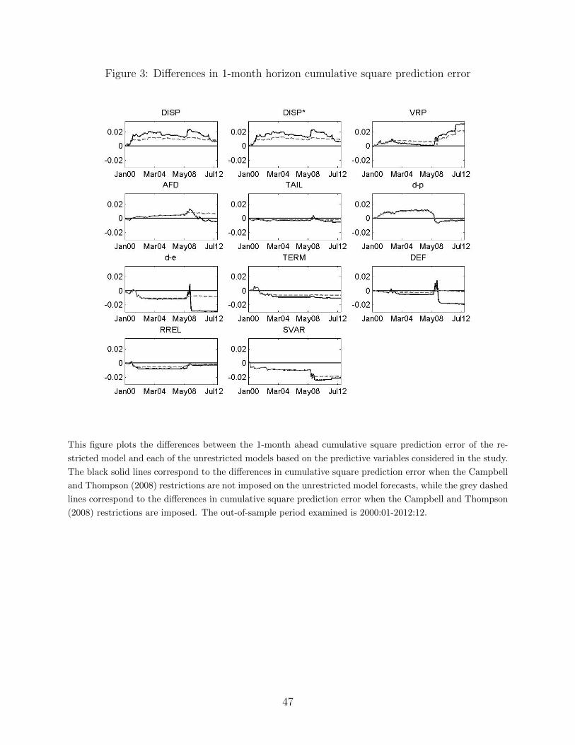
Figure 3: Differences in 1-month horizon cumulative square prediction error

This figure plots the differences between the 1-month ahead cumulative square prediction error of the re-

stricted model and each of the unrestricted models based on the predictive variables considered in the study.

The black solid lines correspond to the differences in cumulative square prediction error when the Campbell

and Thompson (2008) restrictions are not imposed on the unrestricted model forecasts, while the grey dashed

lines correspond to the differences in cumulative square prediction error when the Campbell and Thompson

(2008) restrictions are imposed. The out-of-sample period examined is 2000:01-2012:12.

47

Table 1: Descriptive statistics and correlation coefficients of forecasting variables

Panel A: Descriptive StatisticsDISP DISP* VRP AFD TAIL d-p d-e TERM DEF RREL SVAR

Mean 99.827 132.985 19.306 3.775 0.412 -4.047 -0.860 0.014 0.010 -0.002 0.004Median 100.098 130.693 16.601 3.642 0.415 -4.039 -0.983 0.014 0.009 -0.001 0.002Maximum 220.223 319.493 116.521 5.179 0.501 -3.324 1.379 0.034 0.034 0.011 0.058Minimum 26.898 34.010 -180.679 2.823 0.290 -4.503 -1.244 -0.004 0.006 -0.027 0.000Std. Dev. 32.659 42.940 22.697 0.609 0.038 0.229 0.491 0.011 0.005 0.008 0.006Skewness 0.376 0.504 -2.579 0.430 -0.528 0.276 2.943 0.096 2.779 -0.818 5.910Kurtosis 3.634 4.490 33.137 2.123 3.366 3.595 12.093 1.651 12.374 3.762 48.803AR(1) 0.488 0.505 0.210 0.946 0.612 0.983 0.983 0.984 0.961 0.970 0.695

Panel B: Correlation CoefficientsDISP DISP* VRP AFD TAIL d-p d-e TERM DEF RREL SVAR

DISP 1.00DISP* 0.96 1.00VRP -0.03 -0.07 1.00AFD 0.59 0.61 0.03 1.00TAIL -0.44 -0.42 0.09 -0.41 1.00d-p -0.14 -0.13 -0.07 0.00 -0.06 1.00d-e 0.05 0.01 0.21 -0.02 -0.09 0.51 1.00TERM 0.14 0.14 0.05 0.28 -0.02 0.38 0.37 1.00DEF 0.26 0.24 -0.03 0.25 -0.29 0.66 0.74 0.41 1.00RREL -0.17 -0.12 -0.07 -0.05 -0.01 -0.18 -0.44 -0.35 -0.41 1.00SVAR 0.24 0.22 -0.36 0.05 -0.43 0.34 0.38 0.14 0.59 -0.33 1.00

This table reports descriptive statistics (Panel A) and correlation coefficients (Panel B) of the forecasting variablesused in the study. The forecasting variables are the two dispersion in options traders’ expectations measures (DISP,DISP*), variance risk premium (VRP), analysts’ forecasts dispersion (AFD), tail risk (TAIL), dividend-price ratio(d-p), dividend payout ratio (d-e), yield term spread (TERM), default spread (DEF), relative short-term risk-freerate (RREL) and realized stock market variance (SVAR). The sample period is 1996:01-2012:12.

48

Tab

le2:

On

e-m

onth

hor

izon

pre

dic

tab

ilit

y

Panel

A:

Univ

ari

ate

Panel

B:

Biv

ari

ate

Panel

C:

Tri

vari

ate

R̃2

(%)

DIS

PZ

R̃2

(%)

DIS

P*

ZR̃

2(%

)D

ISP

VR

PZ

R̃2

(%)

DIS

P*

VR

PZ

R̃2

(%)

DIS

P-9

.68

2.23

(-2.

36)*

*[-

2.44

]**

DIS

P*

-9.2

01.

97(-

2.29

)**

[-2.

35]*

*V

RP

16.0

97.

04-9

.27

15.8

59.

10-8

.14

15.5

38.

51(4

.66)

***

(-2.

47)*

*(4

.34)

***

(-2.

24)*

*(4

.28)

***

[2.4

9]**

[-2.

35]*

*[2

.46]

**[-

2.11

]**

[2.4

1]**

AF

D-3

.77

-0.0

8-1

1.42

2.95

1.91

-11.

002.

951.

64-1

0.34

15.7

61.

818.

70-8

.83

15.4

51.

128.

07(-

0.99

)(-

2.02

)**

(0.5

6)(-

1.98

)**

(0.5

6)(-

2.00

)**

(4.2

4)**

*(0

.36)

(-1.

77)*

(4.1

6)**

*(0

.22)

[-0.

98]

[-2.

19]*

*[0

.58]

[-2.

07]*

*[0

.56]

[-2.

01]*

*[2

.45]

**[0

.36]

[-1.

69]*

[2.4

0]**

[0.2

2]T

AIL

4.18

0.01

-9.7

2-0

.10

1.75

-9.0

20.

431.

48-1

0.01

15.9

8-1

.67

8.70

-8.4

415

.58

-0.7

48.

06(0

.93)

(-2.

28)*

*(-

0.02

)(-

2.21

)**

(0.0

9)(-

2.46

)**

(4.3

0)**

*(-

0.40

)(-

2.17

)**

(4.2

3)**

*(-

0.18

)[0

.85]

[-2.

51]*

*[-

0.02

][-

2.39

]**

[0.0

9][-

2.57

]**

[2.4

7]**

[-0.

33]

[-2.

25]*

*[2

.42]

**[-

0.15

]d-p

6.14

0.60

-9.0

14.

912.

44-8

.56

5.05

2.21

-8.4

316

.29

6.10

9.71

-7.3

016

.02

6.30

9.19

(1.0

4)(-

2.09

)**

(0.8

2)(-

2.04

)**

(0.8

5)(-

2.21

)**

(4.5

3)**

*(1

.12)

(-2.

00)*

*(4

.45)

***

(1.1

5)[1

.12]

[-2.

19]*

*[0

.88]

[-2.

11]*

*[0

.90]

[-2.

06]*

*[2

.52]

**[1

.09]

[-1.

83]*

[2.4

8]**

[1.1

3]d-e

1.87

-0.4

0-9

.81

2.37

1.91

-9.2

21.

931.

59-9

.22

16.0

6-1

.00

8.67

-8.1

115

.82

-1.3

78.

10(0

.31)

(-2.

39)*

*(0

.39)

(-2.

28)*

*(0

.32)

(-2.

46)*

*(4

.51)

***

(-0.

17)

(-2.

24)*

*(4

.48)

***

(-0.

23)

[0.3

4][-

2.47

]**

[0.4

3][-

2.36

]**

[0.3

5][-

2.34

]**

[2.4

0]**

[-0.

17]

[-2.

11]*

*[2

.37]

**[-

0.24

]T

ER

M0.

82-0

.48

-10.

012.

271.

89-9

.51

2.17

1.61

-9.4

915

.78

1.45

8.70

-8.3

215

.46

1.27

8.10

(0.2

1)(-

2.40

)**

(0.5

8)(-

2.34

)**

(0.5

5)(-

2.45

)**

(4.3

6)**

*(0

.38)

(-2.

23)*

*(4

.29)

***

(0.3

3)[0

.21]

[-2.

45]*

*[0

.57]

[-2.

37]*

*[0

.55]

[-2.

33]*

*[2

.44]

**[0

.36]

[-2.

10]*

*[2

.39]

**[0

.32]

DE

F-2

.31

-0.3

4-9

.76

0.28

1.75

-9.1

7-0

.15

1.48

-9.4

315

.86

0.59

8.65

-8.1

415

.53

0.00

8.05

(-0.

33)

(-2.

28)*

*(0

.04)

(-2.

21)*

*(-

0.02

)(-

2.33

)**

(4.3

2)**

*(0

.09)

(-2.

10)*

*(4

.26)

***

(0.0

0)[-

0.37

][-

2.34

]**

[0.0

4][-

2.26

]**

[-0.

02]

[-2.

27]*

*[2

.46]

**[0

.09]

[-2.

03]*

*[2

.41]

**[0

.00]

RR

EL

7.35

1.08

-8.7

05.

902.

74-8

.45

6.35

2.64

-8.0

616

.41

7.22

10.1

2-7

.18

16.1

67.

699.

75(1

.57)

(-2.

15)*

*(1

.30)

(-2.

15)*

*(1

.40)

(-2.

14)*

*(4

.18)

***

(1.7

0)*

(-1.

99)*

*(4

.13)

***

(1.8

2)*

[1.7

7]*

[-2.

18]*

*[1

.41]

[-2.

17]*

*[1

.53]

[-2.

04]*

*[2

.52]

**[1

.69]

*[-

1.87

]*[2

.48]

**[1

.81]

*SV

AR

-9.4

02.

08-7

.86

-7.4

93.

29-7

.48

-7.7

43.

15-8

.87

15.2

4-1

.72

8.71

-7.6

714

.71

-2.3

68.

19(-

1.66

)*(-

1.99

)**

(-1.

29)

(-1.

99)*

*(-

1.36

)(-

2.38

)**

(3.2

2)**

*(-

0.29

)(-

2.14

)**

(3.0

9)**

*(-

0.41

)[-

1.23

][-

2.05

]**

[-0.

97]

[-2.

03]*

*[-

1.01

][-

2.32

]**

[2.4

4]**

[-0.

22]

[-2.

08]*

*[2

.36]

**[-

0.31

]

Th

ista

ble

rep

orts

the

resu

lts

of1-

mon

thah

ead

pre

dic

tive

regr

essi

ons

for

the

exce

ssre

turn

onth

eC

RS

Pva

lue-

wei

ghte

din

dex

.T

he

sam

ple

per

iod

is19

96:0

1-20

12:1

2.P

anel

Are

por

tsth

ere

sult

sof

un

ivar

iate

regr

essi

ons,

Pan

elB

the

resu

lts

ofb

ivar

iate

regr

essi

ons

and

Pan

elC

the

resu

lts

oftr

ivar

iate

regr

essi

ons.

Th

efo

reca

stin

gva

riab

les

are

the

two

dis

per

sion

inop

tion

str

ader

s’ex

pec

tati

ons

mea

sure

s(D

ISP

,D

ISP

*),

vari

ance

risk

pre

miu

m(V

RP

),an

alyst

s’fo

reca

sts

dis

per

sion

(AF

D),

tail

risk

(TA

IL),

div

iden

d-p

rice

rati

o(d

-p),

div

iden

dp

ayou

tra

tio

(d-e

),yie

ldte

rmsp

read

(TE

RM

),d

efau

ltsp

read

(DE

F),

rela

tive

shor

t-te

rmri

sk-f

ree

rate

(RR

EL

)an

dre

aliz

edst

ock

mar

ket

vari

ance

(SV

AR

).R

epor

ted

coeffi

cien

tsin

dic

ate

the

per

centa

gean

nu

aliz

edex

cess

retu

rnre

sult

ing

from

aon

est

and

ard

dev

iati

onin

crea

sein

each

pre

dic

tor

vari

able

.N

ewey

and

Wes

t(1

987)

and

Hod

rick

(199

2)t-

stat

isti

csw

ith

lag

len

gth

equ

alto

the

fore

cast

ing

hor

izon

are

rep

orte

din

par

enth

eses

and

squ

are

bra

cket

sre

spec

tive

ly.

***,

**an

d*

den

ote

sign

ifica

nce

atth

e1%

,5%

and

10%

leve

ls.

49

Table 3: Univariate long-horizon predictability

h=3 h=6 h=12 h=24

R̃2 (%) R̃2 (%) R̃2 (%) R̃2 (%)DISP -7.39 3.61 -5.47 3.54 -6.67 10.89 -5.19 12.72

(-2.59)** (-2.25)** (-2.90)*** (-2.35)**[-2.33]** [-1.83]* [-2.38]** [-2.02]**

DISP* -7.10 3.30 -5.10 3.00 -6.65 10.80 -5.20 12.74(-2.65)*** (-2.24)** (-3.03)*** (-2.49)**[-2.31]** [-1.81]* [-2.40]** [-2.11]**

VRP 13.05 12.32 8.34 8.90 3.94 3.46 2.90 3.58(5.25)*** (3.96)*** (2.40)** (2.29)**[3.62]*** [3.33]*** [2.06]** [1.77]*

AFD -4.49 1.02 -5.10 3.01 -5.78 8.04 -5.02 11.88(-1.39) (-1.44) (-1.55) (-1.31)[-1.15] [-1.27] [-1.47] [-1.62]

TAIL -1.21 -0.39 -1.48 -0.22 2.22 0.74 3.58 5.75(-0.38) (-0.49) (0.74) (1.25)[-0.32] [-0.43] [0.77] [1.32]

d-p 6.70 2.88 7.67 7.44 8.23 16.84 8.32 33.56(1.28) (1.84)* (2.72)*** (4.46)***[1.25] [1.50] [1.76]* [1.96]*

d-e 3.42 0.38 4.38 2.09 4.28 4.17 6.10 17.79(0.73) (1.23) (2.26)** (3.25)***[0.67] [0.99] [1.17] [2.18]**

TERM 1.01 -0.43 1.82 -0.06 4.03 3.64 7.55 27.54(0.28) (0.54) (1.38) (3.27)***[0.26] [0.46] [1.05] [2.35]**

DEF -0.27 -0.50 2.07 0.07 3.30 2.27 4.22 8.22(-0.04) (0.45) (1.23) (2.00)**[-0.05] [0.38] [0.78] [1.27]

RREL 7.63 3.89 7.65 7.39 6.53 10.41 -0.58 -0.40(1.95)* (1.94)* (1.59) (-0.33)[1.82]* [1.71]* [1.42] [-0.18]

SVAR -4.88 1.29 0.49 -0.48 2.37 0.92 2.48 2.48(-1.21) (0.20) (2.05)** (2.64)***[-0.93] [0.10] [0.77] [1.19]

This table reports the results of 3-, 6-, 12- and 24-month ahead univariate predictive regressions forthe excess return on the CRSP value-weighted index. The sample period is 1996:01-2012:12. Theforecasting variables are the two dispersion in options traders’ expectations measures (DISP, DISP*),variance risk premium (VRP), analysts’ forecasts dispersion (AFD), tail risk (TAIL), dividend-priceratio (d-p), dividend payout ratio (d-e), yield term spread (TERM), default spread (DEF), relativeshort-term risk-free rate (RREL) and realized stock market variance (SVAR). Reported coefficientsindicate the percentage annualized excess return resulting from a one standard deviation increasein each predictor variable. Newey and West (1987) and Hodrick (1992) t-statistics with lag lengthequal to the forecasting horizon are reported in parentheses and square brackets respectively. ***,** and * denote significance at the 1%, 5% and 10% levels.

50

Tab

le4:

Tri

vari

ate

lon

g-h

oriz

onp

red

icta

bil

ity

Panel

A:

3-m

onth

hori

zon

Panel

B:

6-m

onth

hori

zon

DIS

PV

RP

ZR̃

2(%

)D

ISP

*V

RP

ZR̃

2(%

)D

ISP

VR

PZ

R̃2

(%)

DIS

P*

VR

PZ

R̃2

(%)

AF

D-6

.32

12.9

2-1

.23

15.2

8-5

.11

12.7

6-1

.82

14.5

3-3

.14

8.40

-3.5

812

.87

-1.9

28.

38-4

.26

12.3

1(-

2.37

)**

(4.7

7)**

*(-

0.34

)(-

2.01

)**

(4.7

8)**

*(-

0.49

)(-

1.39

)(3

.88)

***

(-0.

94)

(-0.

80)

(3.9

7)**

*(-

1.03

)[-

1.79

]*[3

.60]

***

[-0.

27]

[-1.

46]

[3.5

5]**

*[-

0.39

][-

1.02

][3

.35]

***

[-0.

78]

[-0.

63]

[3.3

2]**

*[-

0.89

]T

AIL

-10.

1013

.42

-6.9

318

.12

-8.7

513

.01

-6.0

816

.68

-7.9

48.

72-5

.93

15.5

2-6

.82

8.39

-5.2

613

.82

(-3.

74)*

**(5

.87)

***

(-2.

61)*

**(-

3.43

)***

(5.7

0)**

*(-

2.34

)**

(-3.

27)*

**(4

.55)

***

(-2.

07)*

*(-

3.02

)***

(4.3

9)**

*(-

1.89

)*[-

3.31

]***

[3.7

0]**

*[-

1.78

]*[-

2.99

]***

[3.6

1]**

*[-

1.56

][-

2.95

]***

[3.5

8]**

*[-

1.83

]*[-

2.74

]***

[3.4

6]**

*[-

1.61

]d-p

-6.0

913

.32

6.72

18.5

6-5

.30

13.1

36.

8717

.88

-4.1

58.

727.

6219

.47

-3.4

68.

597.

7418

.76

(-2.

34)*

*(6

.10)

***

(1.6

7)*

(-2.

25)*

*(6

.07)

***

(1.7

0)*

(-2.

21)*

*(5

.00)

***

(2.2

2)**

(-2.

04)*

*(4

.97)

***

(2.2

5)**

[-1.

85]*

[3.7

0]**

*[1

.22]

[-1.

69]*

[3.6

5]**

*[1

.26]

[-1.

36]

[3.6

3]**

*[1

.47]

[-1.

21]

[3.6

1]**

*[1

.50]

d-e

-7.1

212

.61

1.18

15.3

1-6

.25

12.4

30.

9014

.43

-5.4

57.

563.

1313

.01

-4.6

37.

432.

9011

.88

(-2.

99)*

**(5

.37)

***

(0.2

9)(-

2.77

)***

(5.3

1)**

*(0

.21)

(-2.

40)*

*(3

.85)

***

(0.8

8)(-

2.14

)**

(3.8

2)**

*(0

.81)

[-2.

27]*

*[3

.44]

***

[0.2

3][-

2.06

]**

[3.4

0]**

*[0

.17]

[-1.

85]*

[2.7

0]**

*[0

.67]

[-1.

66]*

[2.6

6]**

*[0

.62]

TE

RM

-7.2

612

.78

1.45

15.3

6-6

.42

12.5

41.

3214

.50

-5.5

98.

092.

2412

.41

-4.8

67.

912.

1311

.38

(-3.

03)*

**(4

.83)

***

(0.4

6)(-

2.84

)***

(4.8

1)**

*(0

.41)

(-2.

50)*

*(3

.74)

***

(0.7

4)(-

2.24

)**

(3.7

0)**

*(0

.69)

[-2.

23]*

*[3

.55]

***

[0.3

6][-

2.05

]**

[3.4

9]**

*[0

.33]

[-1.

82]*

[3.2

2]**

*[0

.54]

[-1.

69]*

[3.1

6]**

*[0

.52]

DE

F-7

.59

12.9

02.

0615

.51

-6.6

112

.63

1.60

14.5

6-6

.29

8.27

3.91

13.6

8-5

.36

8.06

3.49

12.3

5(-

3.35

)***

(5.2

6)**

*(0

.51)

(-3.

02)*

**(5

.14)

***

(0.3

9)(-

2.79

)***

(4.5

2)**

*(1

.15)

(-2.

43)*

*(4

.38)

***

(1.0

1)[-

2.33

]**

[3.5

9]**

*[0

.33]

[-2.

08]*

*[3

.53]

***

[0.2

6][-

2.08

]**

[3.3

7]**

*[0

.70]

[-1.

87]*

[3.2

8]**

*[0

.63]

RR

EL

-5.7

513

.45

7.65

19.5

1-5

.23

13.2

77.

9719

.11

-3.9

68.

797.

6119

.38

-3.5

58.

677.

8418

.98

(-2.

60)*

*(3

.99)

***

(2.6

0)**

*(-

2.45

)**

(3.9

5)**

*(2

.66)

***

(-1.

56)

(3.0

6)**

*(2

.15)

**(-

1.53

)(3

.04)

***

(2.2

3)**

[-1.

83]*

[3.6

9]**

*[1

.79]

*[-

1.73

]*[3

.65]

***

[1.8

7]*

[-1.

32]

[3.3

8]**

*[1

.65]

[-1.

26]

[3.3

4]**

*[1

.71]

*SV

AR

-7.4

913

.54

1.89

15.4

3-6

.50

13.0

91.

3414

.49

-6.6

810

.35

5.94

15.6

4-5

.66

9.95

5.43

14.0

9(-

3.19

)***

(4.4

3)**

*(0

.59)

(-2.

90)*

**(4

.17)

***

(0.4

1)(-

2.85

)***

(5.8

1)**

*(2

.99)

***

(-2.

53)*

*(5

.65)

***

(2.7

6)**

*[-

2.39

]**

[3.4

0]**

*[0

.33]

[-2.

13]*

*[3

.32]

***

[0.2

3][-

2.26

]**

[3.9

9]**

*[1

.13]

[-2.

03]*

*[3

.90]

***

[1.0

4]

(to

be

conti

nu

ed)

51

(con

tinu

ed)

Panel

C:

12-m

onth

hori

zon

Panel

D:

24-m

onth

hori

zon

DIS

PV

RP

ZR̃

2(%

)D

ISP

*V

RP

ZR̃

2(%

)D

ISP

VR

PZ

R̃2

(%)

DIS

P*

VR

PZ

R̃2

(%)

AF

D-4

.73

4.03

-3.3

315

.68

-4.4

23.

83-3

.41

15.0

3-3

.15

3.08

-3.5

319

.74

-2.9

72.

96-3

.61

19.2

9(-

1.92

)*(2

.35)

**(-

0.90

)(-

1.85

)*(2

.32)

**(-

0.89

)(-

1.93

)*(2

.19)

**(-

1.04

)(-

2.01

)**

(2.1

3)**

(-1.

04)

[-2.

03]*

*[2

.05]

**[-

0.81

][-

2.01

]**

[1.9

5]*

[-0.

82]

[-1.

87]*

[1.8

3]*

[-1.

28]

[-1.

95]*

[1.7

5]*

[-1.

27]

TA

IL-7

.46

3.97

-1.7

814

.34

-7.1

33.

62-1

.50

13.5

2-4

.55

2.64

1.21

16.0

4-4

.40

2.42

1.36

15.6

2(-

3.88

)***

(2.4

3)**

(-0.

68)

(-3.

98)*

**(2

.21)

**(-

0.59

)(-

2.69

)***

(1.8

5)*

(0.5

1)(-

2.72

)***

(1.6

9)*

(0.5

8)[-

3.11

]***

[2.1

9]**

[-0.

73]

[-3.

03]*

**[2

.00]

**[-

0.61

][-

2.25

]**

[1.7

0]*

[0.5

5][-

2.37

]**

[1.5

4][0

.62]

d-p

-5.2

14.

307.

5327

.87

-4.9

94.

077.

5527

.28

-3.3

33.

277.

7643

.82

-3.1

53.

137.

7843

.25

(-3.

18)*

**(2

.86)

***

(3.0

6)**

*(-

3.05

)***

(2.7

1)**

*(2

.99)

***

(-3.

55)*

**(2

.16)

**(6

.80)

***

(-3.

52)*

**(2

.04)

**(6

.40)

***

[-1.

82]*

[2.3

6]**

[1.5

9][-

1.77

]*[2

.28]

**[1

.59]

[-1.

28]

[2.1

5]**

[1.8

0]*

[-1.

27]

[2.0

9]**

[1.8

0]*

d-e

-7.0

02.

934.

2918

.26

-6.6

62.

684.

0517

.12

-6.0

21.

336.

6135

.89

-5.7

61.

116.

4534

.41

(-3.

27)*

**(1

.70)

*(1

.95)

*(-

3.14

)***

(1.5

5)(1

.80)

*(-

3.72

)***

(1.0

1)(3

.69)

***

(-3.

47)*

**(0

.82)

(3.6

7)**

*[-

2.52

]**

[1.3

9][1

.13]

[-2.

44]*

*[1

.28]

[1.0

6][-

2.37

]**

[0.7

5][2

.26]

**[-

2.37

]**

[0.6

3][2

.21]

**T

ER

M-7

.25

3.57

4.83

19.6

4-7

.06

3.25

4.79

18.9

0-6

.01

2.16

8.06

47.3

1-5

.71

1.91

7.90

45.5

9(-

3.53

)***

(2.1

4)**

(2.0

5)**

(-3.

55)*

**(1

.93)

*(1

.93)

*(-

4.18

)***

(1.6

1)(4

.35)

***

(-3.

89)*

**(1

.39)

(4.1

6)**

*[-

2.52

]**

[1.8

7]*

[1.2

3][-

2.51

]**

[1.7

2]*

[1.2

3][-

2.29

]**

[1.3

2][2

.46]

**[-

2.29

]**

[1.1

7][2

.42]

**D

EF

-7.9

53.

905.

3820

.74

-7.5

23.

555.

0219

.29

-6.5

82.

865.

9331

.93

-6.2

42.

585.

6630

.10

(-3.

82)*

**(2

.61)

***

(2.7

8)**

*(-

3.62

)***

(2.3

6)**

(2.5

7)**

(-3.

64)*

**(2

.06)

**(4

.31)

***

(-3.

40)*

**(1

.85)

*(4

.11)

***

[-2.

84]*

**[2

.08]

**[1

.25]

[-2.

73]*

**[1

.91]

*[1

.17]

[-2.

59]*

*[1

.78]

*[1

.78]

*[-

2.58

]**

[1.6

0][1

.71]

*R

RE

L-5

.49

4.25

5.78

22.0

3-5

.50

4.01

6.01

22.1

5-5

.42

2.63

-1.5

016

.55

-5.2

22.

41-1

.26

15.6

5(-

2.01

)**

(1.9

3)*

(1.4

6)(-

2.17

)**

(1.8

4)*

(1.5

4)(-

2.50

)**

(1.9

2)*

(-0.

88)

(-2.

47)*

*(1

.74)

*(-

0.74

)[-

1.99

]**

[2.0

9]**

[1.2

3][-

2.03

]**

[1.9

8]**

[1.2

8][-

2.16

]**

[1.5

1][-

0.47

][-

2.17

]**

[1.3

9][-

0.39

]SV

AR

-8.5

66.

427.

1424

.16

-8.0

75.

906.

7122

.45

-6.7

14.

946.

1230

.38

-6.4

14.

555.

8628

.75

(-3.

90)*

**(3

.82)

***

(4.2

3)**

*(-

3.79

)***

(3.8

1)**

*(4

.31)

***

(-3.

85)*

**(3

.05)

***

(3.7

7)**

*(-

3.57

)***

(3.0

4)**

*(3

.91)

***

[-3.

00]*

**[3

.02]

***

[2.1

2]**

[-2.

87]*

**[2

.84]

***

[1.9

9]**

[-2.

64]*

**[2

.55]

**[2

.66]

***

[-2.

65]*

**[2

.37]

**[2

.55]

**

Th

ista

ble

rep

orts

the

resu

lts

of3-

(Pan

elA

),6-

(Pan

elB

),12

-(P

anel

C)

and

24-m

onth

(Pan

elD

)ah

ead

triv

aria

tep

red

icti

vere

gres

sion

sfo

rth

eex

cess

retu

rnon

the

CR

SP

valu

e-w

eigh

ted

ind

ex.

Th

esa

mp

lep

erio

dis

1996

:01-

2012

:12.

Th

efo

reca

stin

gva

riab

les

are

the

two

dis

per

sion

inop

tion

str

ader

s’ex

pec

tati

ons

mea

sure

s(D

ISP

,D

ISP

*),

vari

ance

risk

pre

miu

m(V

RP

),an

alyst

s’fo

reca

sts

dis

per

sion

(AF

D),

tail

risk

(TA

IL),

div

iden

d-p

rice

rati

o(d

-p),

div

iden

dp

ayou

tra

tio

(d-e

),yie

ldte

rmsp

read

(TE

RM

),d

efau

ltsp

read

(DE

F),

rela

tive

shor

t-te

rmri

sk-f

ree

rate

(RR

EL

)an

dre

aliz

edst

ock

mar

ket

vari

ance

(SV

AR

).R

epor

ted

coeffi

cien

tsin

dic

ate

the

per

centa

gean

nu

aliz

edex

cess

retu

rnre

sult

ing

from

aon

est

and

ard

dev

iati

onin

crea

sein

each

pre

dic

tor

vari

able

.N

ewey

and

Wes

t(1

987)

and

Hod

rick

(199

2)t-

stat

isti

csw

ith

lag

len

gth

equ

alto

the

fore

cast

ing

hor

izon

are

rep

orte

din

par

enth

eses

and

squ

are

bra

cket

sre

spec

tive

ly.

***,

**an

d*

den

ote

sign

ifica

nce

atth

e1%

,5%

and

10%

leve

ls.

52

Tab

le5:

Out-

of-s

ample

pre

dic

tabilit

y

1-m

onth

hori

zon

3-m

onth

hori

zon

6-m

onth

hori

zon

R2 OS

(%)

MS

E-F

MS

E-A

dj

R2 COS

(%)

R2 OS

(%)

MS

E-F

MS

E-A

dj

R2 COS

(%)

R2 OS

(%)

MS

E-F

MS

E-A

dj

R2 COS

(%)

DIS

P1.

702.

69**

1.69

**2.

163.

375.

29**

1.69

**4.

931.

392.

05**

1.29

*7.

19D

ISP

*1.

552.

46**

1.63

*2.

443.

044.

77**

1.70

**4.

821.

091.

61**

1.36

*6.

36V

RP

7.96

13.5

0**

2.40

**5.

6112

.47

21.6

6**

3.25

**13

.22

8.76

14.0

2**

2.98

**13

.05

AF

D-1

.24

-1.9

10.

311.

64-3

.04

-4.4

80.

543.

72-1

0.28

-13.

610.

295.

97T

AIL

-1.3

9-2

.14

-0.2

2-0

.47

-5.4

3-7

.83

-1.8

4-4

.44

-9.9

9-1

3.26

-1.5

7-7

.62

d-p

-0.7

1-1

.10

0.45

-0.5

4-3

.81

-5.5

80.

11-3

.90

-2.8

8-4

.09

0.40

-2.9

3d

-e-7

.60

-11.

01-0

.12

-2.1

3-3

5.49

-39.

81-0

.96

-8.2

4-8

3.24

-66.

33-1

.74

-42.

80T

ER

M-2

.71

-4.1

2-0

.48

-1.7

0-1

2.27

-16.

61-1

.01

-9.9

6-3

2.81

-36.

07-1

.32

-28.

44D

EF

-4.9

1-7

.30

0.47

-0.3

4-2

4.50

-29.

910.

061.

78-6

6.88

-58.

51-0

.59

5.79

RR

EL

-0.6

8-1

.05

0.21

-0.4

1-3

.83

-5.6

10.

09-3

.99

-14.

19-1

8.14

-0.2

7-1

3.57

SV

AR

-5.3

9-7

.97

0.35

-4.7

5-1

3.05

-17.

55-1

.93

-10.

32-7

.21

-9.8

1-1

.32

-3.5

7D

ISP

&V

RP

9.06

15.5

4**

2.76

**4.

0715

.15

27.1

4**

3.20

**12

.36

11.2

718

.55*

*3.

11**

15.7

8D

ISP

*&

VR

P8.

5614

.60*

*2.

70**

4.10

14.3

425

.45*

*3.

23**

12.1

310

.36

16.8

7**

3.13

**15

.12

This

table

rep

orts

the

resu

lts

of1-

,3-

and

6-m

onth

ahea

dou

t-of

-sam

ple

pre

dic

tabilit

yfo

rth

eex

cess

retu

rnon

the

CR

SP

valu

e-w

eigh

ted

index

.T

he

tota

lsa

mple

per

iod

is19

96:0

1-20

12:1

2an

dth

efo

reca

stin

gp

erio

db

egin

sin

2000

:01.

The

fore

cast

ing

vari

able

sar

eth

etw

odis

per

sion

inop

tion

str

ader

s’ex

pec

tati

ons

mea

sure

s(D

ISP

,D

ISP

*),

vari

ance

risk

pre

miu

m(V

RP

),an

alyst

s’fo

reca

sts

dis

per

sion

(AF

D),

tail

risk

(TA

IL),

div

iden

d-p

rice

rati

o(d

-p),

div

iden

dpay

out

rati

o(d

-e),

yie

ldte

rmsp

read

(TE

RM

),def

ault

spre

ad(D

EF

),re

lati

vesh

ort-

term

risk

-fre

era

te(R

RE

L)

and

real

ized

stock

mar

ket

vari

ance

(SV

AR

).R

2 OS

isth

eou

t-of

-sam

ple

coeffi

cien

tof

det

erm

inat

ion,

MSE

-Fis

the

McC

rack

en(2

007)

F-s

tati

stic

,M

SE

-Adj

isth

eM

SE

-Adju

sted

stat

isti

cof

Cla

rkan

dW

est

(200

7)an

dR

2 COS

isth

eou

t-of

-sam

ple

coeffi

cien

tof

det

erm

inat

ion

when

the

out-

of-s

ample

pre

dic

tion

isre

stri

cted

tob

ep

osit

ive.

**an

d*

den

ote

sign

ifica

nce

atth

e5%

and

10%

leve

ls.

53

Table 6: Market-timing strategy with mean-variance weights

Mean (%) St. Dev. (%) Sharpe ∆CER (%) MDD (%) Long (%)Buy & Hold 4.76 25.15 0.19 -67.86DISP 3.34 10.14 0.33 6.54 -27.18 55.77DISP* 3.40 10.00 0.34 6.63 -22.10 52.56VRP 6.17 15.71 0.39 7.21 -44.13 55.77AFD 3.04 10.16 0.30 6.22 -40.73 69.87TAIL -1.28 11.96 -0.11 1.31 -52.19 83.97d-p 5.71 18.72 0.31 5.19 -62.19 96.79d-e 2.62 11.20 0.23 5.48 -40.95 82.69TERM -0.62 12.04 -0.05 1.94 -38.30 84.62DEF -0.50 11.53 -0.04 2.25 -42.49 77.56RREL 2.30 11.59 0.20 5.02 -46.56 88.46SVAR -1.37 15.86 -0.09 -0.41 -53.74 91.03DISP & VRP 6.53 13.73 0.48 8.44 -28.33 56.41DISP* & VRP 5.61 13.72 0.41 7.52 -28.10 51.92

This table reports the results of market-timing strategies with mean-variance weights based on the1-month ahead out-of-sample predictability for the excess return on the CRSP value-weighted index.The total sample period is 1996:01-2012:12 and the forecasting period begins in 2000:01. Panel A showsthe results when short sales are not allowed and Panel B when short sales are allowed. The forecastingvariables are the two dispersion in options traders’ expectations measures (DISP, DISP*), variancerisk premium (VRP), analysts’ forecasts dispersion (AFD), tail risk (TAIL), dividend-price ratio (d-p),dividend payout ratio (d-e), yield term spread (TERM), default spread (DEF), relative short-term risk-free rate (RREL) and realized stock market variance (SVAR). Buy & Hold refers to a passive strategythat takes a long position on the market portfolio. Mean denotes the average return, St. Dev. denotesthe standard deviation of returns, Sharpe stands for the Sharpe ratio, ∆CER is the certainty equivalentreturn in excess of the buy-hold strategy, MDD stands for the maximum drawdown, and Long is thepercentage of months that the strategy takes a long position on the market index. All measures ofperformance apart from MDD are in annualized terms.

54

Table 7: Market-timing strategy with binary weights

Mean (%) St. Dev. (%) Sharpe ∆CER (%) MDD (%) Long (%)Panel A: No short sales

Buy & Hold 3.88 16.75 0.23 -51.44DISP 5.46 9.41 0.58 4.46 -14.09 55.77DISP* 2.62 9.59 0.27 1.58 -24.06 52.56VRP 6.93 12.81 0.54 4.80 -32.24 55.77AFD -0.52 12.99 -0.04 -2.72 -44.87 69.87TAIL 2.50 13.26 0.19 0.20 -46.24 83.97d-p 3.99 16.44 0.24 0.27 -51.44 96.79d-e 6.39 12.44 0.51 4.40 -27.70 82.69TERM 1.63 14.31 0.11 -1.11 -47.30 84.62DEF 4.43 12.75 0.35 2.33 -33.35 77.56RREL 3.53 14.38 0.25 0.76 -52.82 88.46SVAR 3.99 15.03 0.27 0.94 -44.87 91.03DISP & VRP 10.98 11.38 0.96 9.37 -19.95 56.41DISP* & VRP 9.57 11.34 0.84 7.97 -19.95 51.92

Panel B: Short salesBuy & Hold 4.76 25.15 0.19 -67.86DISP 7.91 15.74 0.50 8.93 -29.02 55.77DISP* 2.25 15.98 0.14 3.15 -48.50 52.56VRP 10.85 19.93 0.54 9.63 -41.02 55.77AFD -4.04 20.18 -0.20 -5.41 -66.24 69.87TAIL 2.00 20.57 0.10 0.39 -64.12 83.97d-p 4.98 24.73 0.20 0.54 -69.24 96.79d-e 9.78 19.47 0.50 8.83 -40.59 82.69TERM 0.27 21.93 0.01 -2.21 -68.21 84.62DEF 5.87 19.92 0.29 4.66 -48.66 77.56RREL 4.06 22.02 0.18 1.52 -72.65 88.46SVAR 4.99 22.87 0.22 1.88 -62.26 91.03DISP & VRP 18.97 17.89 1.06 18.90 -22.74 56.41DISP* & VRP 16.14 17.93 0.90 16.05 -22.74 51.92

This table reports the results of market-timing strategies with binary weights based on the 1-monthahead out-of-sample predictability for the excess return on the CRSP value-weighted index. The totalsample period is 1996:01-2012:12 and the forecasting period begins in 2000:01. Panel A shows the resultswhen short sales are not allowed and Panel B when short sales are allowed. The forecasting variablesare the two dispersion in options traders’ expectations measures (DISP, DISP*), variance risk premium(VRP), analysts’ forecasts dispersion (AFD), tail risk (TAIL), dividend-price ratio (d-p), dividend payoutratio (d-e), yield term spread (TERM), default spread (DEF), relative short-term risk-free rate (RREL)and realized stock market variance (SVAR). Buy & Hold refers to a passive strategy that takes a longposition on the market portfolio. Mean denotes the average return, St. Dev. denotes the standarddeviation of returns, Sharpe stands for the Sharpe ratio, ∆CER is the certainty equivalent return inexcess of the buy-hold strategy, MDD stands for the maximum drawdown, and Long is the percentageof months that the strategy takes a long position on the market index. All measures of performanceapart from MDD are in annualized terms.

55

Table 8: Portfolio rotation strategies

Mean (%) St. Dev. (%) Sharpe ∆CER (%) MDD (%) Long (%)Panel A: Portfolio Strategies for DISP and DISP*

Buy & Hold 4.76 25.15 0.19 -67.86

DISPSize 10.02 20.56 0.49 8.41 -39.47 76.92B/M 2.00 17.97 0.11 1.90 -51.42 87.18Mom 5.31 20.02 0.27 4.03 -43.06 86.54Industry 3.53 22.70 0.16 0.54 -62.41 100.00LT Reversal 8.51 21.72 0.39 6.17 -43.69 92.95ST Reversal 8.62 18.07 0.48 8.46 -45.72 84.62Pooled 8.11 24.93 0.33 3.52 -51.61 100.00

DISP*Size 8.90 20.62 0.43 7.26 -34.01 75.64B/M -0.58 17.36 -0.03 -0.36 -50.25 86.54Mom 3.45 19.76 0.17 2.33 -40.77 83.97Industry 3.24 21.98 0.15 0.73 -63.31 100.00LT Reversal 6.73 22.24 0.30 4.04 -46.64 93.59ST Reversal 9.47 17.64 0.54 9.54 -27.02 82.69Pooled 8.12 23.82 0.34 4.34 -43.69 100.00

Panel B: Pooled Portfolio Strategies for Alternative PredictorsVRP 18.51 28.87 0.64 10.74 -57.34 100.00AFD 7.58 25.88 0.29 2.27 -50.53 100.00TAIL 1.54 25.81 0.06 -3.72 -73.21 100.00d-p 3.38 33.60 0.10 -8.83 -76.54 100.00d-e 5.50 30.43 0.18 -3.65 -75.11 96.79TERM 8.07 29.57 0.27 -0.31 -64.15 100.00DEF 2.57 28.56 0.09 -4.93 -76.33 96.15RREL -3.08 27.85 -0.11 -9.98 -82.69 100.00SVAR 4.09 29.22 0.14 -3.99 -68.04 96.15

This table reports the results of portfolio rotation strategies based on the 1-month ahead out-of-sample predictability for the excess stock portfolio returns. The total sample period is 1996:01-2012:12 and the forecasting period begins in 2000:01. The forecasting variables are the two dispersionin options traders’ expectations measures (DISP, DISP*), variance risk premium (VRP), analysts’forecasts dispersion (AFD), tail risk (TAIL), dividend-price ratio (d-p), dividend payout ratio (d-e),yield term spread (TERM), default spread (DEF), relative short-term risk-free rate (RREL) andrealized stock market variance (SVAR). Buy & Hold refers to a passive strategy that takes a longposition on the market portfolio. Mean denotes the average return, St. Dev. denotes the standarddeviation of returns, Sharpe stands for the Sharpe ratio, ∆CER is the certainty equivalent return inexcess of the buy-hold strategy, MDD stands for the maximum drawdown and Long is the percentageof months that the strategy takes a long position on the two winner portfolios. All measures ofperformance apart from MDD are in annualized terms. The rotation strategies use decile portfoliossorted on size (Size), book-market ratio (B/M), momentum (Mom), industry (Industry), long-termreversal (LT Reversal) and short-term reversal (ST Reversal). Pooled refers to a rotation strategythat uses all 60 portfolios. Panel A shows the results of the rotation strategies based on the forecastingperformance of the dispersion in options’ traders expectations, while Panel B shows the results ofthe rotation strategies using all 60 portfolios based on the forecasting performance of the alternativepredictors.

56

Table 9: Comparison with other option-implied measures – One-month horizon

Panel A: Correlation CoefficientsSlope HP VIX Skewness Kurtosis

DISP 0.18 -0.24 0.29 -0.02 0.05DISP* 0.19 -0.25 0.23 -0.09 0.12

Panel B: Bivariate RegressionsSlope HP VIX Skewness Kurtosis

DISP -9.95 -9.80 -10.89 -9.67 -9.68(-2.39)** (-2.27)** (-2.73)*** (-2.35)** (-2.34)**[-2.44]** [-2.37]** [-2.78]*** [-2.43]** [-2.42]**

Z 1.53 -0.51 4.14 0.72 0.00(0.34) (-0.12) (0.64) (0.17) (0.00)[0.33] [-0.12] [0.70] [0.18] [0.00]

R̃2 (%) 1.81 1.75 2.20 1.76 1.75

DISP* -9.48 -9.33 -9.97 -9.20 -9.28(-2.30)** (-2.17)** (-2.59)** (-2.24)** (-2.24)**[-2.34]** [-2.26]** [-2.63]*** [-2.30]** [-2.29]**

Z 1.52 -0.52 3.30 0.07 0.64(0.33) (-0.12) (0.52) (0.02) (0.16)[0.33] [-0.12] [0.56] [0.02] [0.17]

R̃2 (%) 1.55 1.49 1.78 1.48 1.49

Panel C: Multivariate Regressions

DISP Slope HP VIX Skewness Kurtosis R̃2 (%)-11.51 3.07 0.25 3.90 9.75 8.54 0.52

(-2.65)*** (0.50) (0.06) (0.55) (0.86) (0.87)[-2.72]*** [0.50] [0.06] [0.59] [0.84] [0.90]

DISP* Slope HP VIX Skewness Kurtosis R̃2 (%)-10.59 2.48 0.15 3.27 8.26 8.00 0.05

(-2.41)** (0.41) (0.03) (0.47) (0.73) (0.82)[-2.49]** [0.41] [0.03] [0.50] [0.72] [0.85]

This table reports the results of 1-month ahead predictive regressions for the excess return onthe CRSP value-weighted index. The sample period is 1996:01-2012:12. Panel A reports thecorrelation coefficients, Panel B the results of bivariate regressions and Panel C the results ofmultivariate regressions. The forecasting variables are the two dispersion in options traders’expectations measures (DISP, DISP*), slope of the implied volatility curve (Slope), hedgingpressure (HP), implied volatility (VIX), risk-neutral skewness (Skewness) and risk-neutralkurtosis (Kurtosis). Reported coefficients indicate the percentage annualized excess returnresulting from a one standard deviation increase in each predictor variable. Newey and West(1987) and Hodrick (1992) t-statistics with lag length equal to the forecasting horizon arereported in parentheses and square brackets respectively. ***, ** and * denote significanceat the 1%, 5% and 10% levels.

57

Table 10: Comparison with other option-implied measures – Long horizons

Panel A: Multivariate model with DISP

DISP Slope HP VIX Skewness Kurtosis R̃2

h=3 -8.66 2.29 3.40 6.06 -5.93 -4.16 6.89(-3.09)*** (0.66) (1.36) (1.04) (-0.67) (-0.45)[-2.58]** [0.56] [1.20] [1.15] [-0.71] [-0.56]

h=6 -7.63 1.64 2.59 7.95 -0.34 2.87 11.48(-3.00)*** (0.71) (1.34) (2.89)*** (-0.06) (0.44)[-2.53]** [0.54] [1.09] [1.77]* [-0.06] [0.53]

h=12 -8.68 1.33 2.06 7.07 2.86 5.67 23.11(-4.01)*** (1.11) (1.56) (3.29)*** (0.52) (0.86)[-3.14]*** [0.67] [1.06] [2.36]** [0.58] [1.21]

h=24 -7.65 3.23 0.82 6.08 9.73 8.34 33.23(-4.35)*** (2.54)** (0.49) (2.82)*** (2.57)** (2.38)**[-3.06]*** [2.42]** [0.53] [2.47]** [1.63] [1.46]

Panel B: Multivariate model with DISP*

DISP* Slope HP VIX Skewness Kurtosis R̃2

h=3 -8.01 1.87 3.32 5.60 -7.03 -4.55 6.25(-2.88)*** (0.55) (1.31) (0.97) (-0.79) (-0.49)[-2.43]** [0.46] [1.16] [1.07] [-0.84] [-0.61]

h=6 -6.88 1.24 2.56 7.50 -1.33 2.47 10.29(-2.73)*** (0.54) (1.26) (2.75)*** (-0.22) (0.38)[-2.43]** [0.42] [1.06] [1.67]* [-0.22] [0.46]

h=12 -8.33 0.93 1.84 6.70 1.79 5.34 22.19(-3.98)*** (0.77) (1.35) (3.22)*** (0.32) (0.81)[-3.05]*** [0.48] [0.95] [2.24]** [0.36] [1.14]

h=24 -7.20 2.94 0.67 5.70 8.94 8.01 30.93(-4.43)*** (2.52)** (0.39) (2.75)*** (2.28)** (2.25)**[-3.06]*** [2.33]** [0.43] [2.32]** [1.51] [1.40]

This table reports the results of 3-, 6-, 12- and 24-month ahead multivariate predictiveregressions for the excess return on the CRSP value-weighted index. The sample periodis 1996:01-2012:12. Panel A reports the results of multivariate regressions with DISP andPanel B the results of multivariate regressions with DISP*. The forecasting variables arethe two dispersion in options traders’ expectations measures (DISP, DISP*), slope of theimplied volatility curve (Slope), hedging pressure (HP), implied volatility (VIX), risk-neutralskewness (Skewness) and risk-neutral kurtosis (Kurtosis). Reported coefficients indicate thepercentage annualized excess return resulting from a one standard deviation increase in eachpredictor variable. Newey and West (1987) and Hodrick (1992) t-statistics with lag lengthequal to the forecasting horizon are reported in parentheses and square brackets respectively.***, ** and * denote significance at the 1%, 5% and 10% levels.

58

Appendix to “Dispersion in Options Traders’Expectations and Stock Return Predictability”

Not for publication

April 2015

Abstract

This appendix includes additional results not presented in the main body of the paper.

1 Results for Additional Predictors

In this section, we provide the results from the main empirical analysis using a series of

additional predictors. In particular, the precitive variables considered are the yield gap

(YG, Maio, 2013), the consumption-wealth ratio (CAY, Lettau and Ludvigson, 2001), the

stock market illiquidity (ILLIQ, Amihud, 2002), and the idiosyncratic risk (IRISK, Goyal

and Santa-Clara, 2003). YG is the difference between the aggregate earnings-price ratio

and the 10-year bond yield, both in levels. CAY is defined as the trend deviation between

consumption, labor income and asset wealth after estimating their cointegrating relationship.

ILLIQ is the cross-sectional average of the individual stock illiquidity measures calculated as

the average of the daily ratio of the absolute return to dollar trading volume using data for

a given month. IRISK is the cross-sectional average of the individual stock return variance

calculated using daily return data for one month. Data on monthly market prices and

earnings are obtained from Robert Shiller’s website. Interest rate data are obtained from the

FRED database of the Federal Reserve Bank of St. Louis. CAY is downloaded from Martin

Lettau’s website.1 Individual stock data - for NYSE firms when calculating ILLIQ and

NYSE/AMEX/NASDAQ firms when calculating IRISK - are downloaded from the Center

for Research in Security Prices (CRSP).

The results from the in-sample (IS) analysis are presented in Tables 1-3. It can be seen

that in our sample period, only the yield gap appears to exhibit some modest predictive

ability and only when combined with DISP (or DISP*) and VRP in trivariate models. More

importantly, the inclusion of any of the additional predictors in the forecasting model has

very limited impact on the significance of the dispersion in options traders’ beliefs measures.

Table 4 reports the results from the out-of-sample (OS) analysis. For completeness we also

report OS results for CAY even though the data provided by Martin Lettau utilize parameters

estimated using the whole sample period and thus suffer from look-ahead bias. Unlike the

dispersion in options traders’ expectations, the alternative variables exhibit negative R2OS

1We create a monthly CAY time-series by using the most recent quarterly observation.

1

values, while CAY and ILLIQ provide positive R2COS values but lower than those of DISP and

DISP*. Moreover, the null hypothesis is rejected only when considering the MSE-Adj test

for the YG.2 Turning to the economic significance of the additional predictors, Tables 5-6

show that the respective trading strategies rarely perform better than the buy-hold strategy

and they almost always underperform the strategies associated with the dispersion in options

traders’ expectations.

2 Results with Bootstrapped P-values

In this section, we provide in-sample predictability results based on empirical p-values ob-

tained from a bootstrap experiment. This method accounts for the high persistence of several

predictive variables and the cross-correlation between the residuals of the predictive regres-

sions and the innovations in the predictive variables (Stambaugh, 1999). The bootstrap

algorithm can be described as follows:

1. We estimate the predictive regressions using OLS and save the slope estimates for

each predictor. We further estimate the OLS coefficients from a regression that imposes the

null hypothesis of no predictability and a first-order autoregression for each predictor. The

respective residuals and estimated regression coefficients are stored.

2. For each replication m=1,...,10000, we build up pseudo-samples for the innovations in

the excess market return and in each of the predictive variables by drawing with replacement

from the residual time series. To preserve the correlation between the predictors and the

return disturbances that drives the Stambaugh (1999) bias the pseudo-samples are created

using the same random time sequence.

3. For each replication, we use the constructed residuals pseudo-samples and the stored

OLS coefficients from step (1) to create a time-series of excess market returns under the

null of no predictability and the respective time series of the predictors under a first-order

2While this result seems paradoxical at a first glance since the R2OS of YG is consistently negative, it can

be explained by the adjustment that the MSE-Adj test imposes to account for the fact that the MSE of theunrestricted model is expected to be higher than the MSE of the restricted model under the null hypothesis.

2

autoregression model. The initial value for each first-order autoregression model is selected

randomly by the original sample.

4. We estimate the predictive regressions using the bootstrapped variables and keep the

slope estimated for each predictor. This results in a sample of 10000 observations for each

slope coefficient.

5. Finally, for each predictive variable we compute the proportion of the bootstrapped

slope coefficients that exceed in absolute terms the respective original coefficient estimated

in step (1). The estimated values represent the respective p-values.

The results from the in-sample analysis when statistical inference is based on boot-

strapped p-values are presented in Tables 7-9. Similarly to the main results, the dispersion

in options traders’ expectations is almost universally significant and none of the alternative

predictive variables appear to subsume its forecasting power.

3 Alternative Out-of-Sample Performance Measure

In this section, we examine the out-of-sample performance of the forecasting variables using

the encompassing test of Clark and McCracken (2001):

ENC −NEW =(TOS − h + 1)

TOS∑T−hs=s0

[(res+h − r̂es+h)2 − (res+h − r̂es+h) (res+h − r̃es+h)

]MSEU

, (1)

which examines whether the restricted model encompasses the unrestricted model, meaning

that the unrestricted model does not improve the forecasting ability of the restricted model.

The results are presented in Table 10 and rely on critical values provided by Clark

and McCracken (2001). The null hypothesis that the restricted model encompasses the

unrestricted model with the dispersion in options traders’ expectations is rejected at 5%

level for all horizons examined.

3

4 Alternative Portfolio Rotation Strategies

In this section, we present the results from two alternative portfolio rotation strategies.

Following Maio (2014), the first one (Table 11) can be considered a myopic rotation strategy

since the investor always invests in the two highest fitted excess return portfolios even if the

respective forecasted returns are negative. In particular, the realized return of the portfolio

rotation strategy can be represented by:

Rp,s+1 = 0.75RH1,s+1 + 0.75RH2,s+1 − 0.25RL1,s+1 − 0.25RL2,s+1 (2)

where RH1,s+1 and RH2,s+1 (RL1,s+1 and RL2,s+1) stand for the realized arithmetic returns of

the portfolios with the highest and second highest (lowest and second lowest) fitted excess

return.

The second rotation strategy (Table 12) examines the robustness of the main rotation

strategies using alternative weights of 130% and -30% instead of 150% and -50% respectively.

More specifically, the realized return of this alternative portfolio rotation strategy is:

Rp,s+1 =

0.65RH1,s+1 + 0.65RH2,s+1 − 0.15RL1,s+1 − 0.15RL2,s+1, if r̂eH1,s+1 ≥ 0

1.3Rf,s+1 − 0.15RL1,s+1 − 0.15RL2,s+1, if r̂eH1,s+1 < 0,

(3)

where r̂eH1,s+1 denotes the highest fitted excess portfolio return.

The results for the dispersion in beliefs measures are qualitatively very similar to those

obtained from the rotation strategies presented in the main body of the paper. For example,

in all but one case (DISP* for B/M portfolios when using the alternative weights) the disper-

sion in options traders’ expectations is associated with positive ∆CER estimates meaning

that it offers additional utility to a mean-variance investor who would otherwise follow a

simple buy-hold strategy. Moreover, when pooling all portfolios together VRP and AFD are

the only other variables that exhibit positive ∆CER estimates, with VRP outperforming the

4

dispersion in options traders’ expectations and AFD mostly underperforming it.

5 Alternative Dispersion in Options Traders’ Expecta-

tions Measures

In this section, we provide in-sample and out-of-sample univariate regression results for

four alternative dispersion measures. In particular, DISPI and DISP*I are constructed using

options of all available moneynesses, DISPII and DISP*II are constructed using only options

that expire in the subsequent month,3 DISPIII and DISP*III are created using options with

maturities between 10 and 60 calendar days and DISPIV and DISP*IV are created using

options with maturities between 10 and 180 calendar days.

Table 13 shows that the in-sample results are qualitatively similar to those obtained for

the main dispersion in expectations variables. In particular, all alternative dispersion mea-

sures exhibit similar statistical significance with slightly lower coefficients of determination

at long horizons. Table 14 shows the respective out-of-sample results. At the 1-month hori-

zon, all alternative dispersion variables provide positive R2OS estimates and the MSE-F and

MSE-Adjusted tests reject the respective null hypotheses at either 5% or 10% level. Turning

to longer horizons, the R2OS values are also positive in all cases apart from DISPI and DISP*

I

at the 6-month horizon. The MSE-F and MSE-Adjusted statistics are most of the times

lower than in the 1-month horizon (in line with the in-sample results discussed before), but

still reject the respective null hypotheses in about half of the cases.

3For consistency across the sample period we include only options that expire on the Saturday after thethird Friday of each month.

5

References

[1] Amihud, Y. 2002. Illiquidity and stock returns: cross-section and time-series effects.Journal of Financial Markets 5, 31-56.

[2] Clark, T. and M. McCracken. 2001. Tests of equal forecast accuracy and encompassingfor nested models. Journal of Econometrics 105, 85-110.

[3] Goyal, A. and P. Santa-Clara. 2003. Idiosyncratic risk matters! Journal of Finance 58,975-1008.

[4] Lettau, M. and S. Ludvigson. 2001. Consumption, aggregate wealth, and expected stockreturns, Journal of Finance 56, 815-849.

[5] Maio, P. 2013. The “FED model” and the predictability of stock returns. Review ofFinance 17, 1489-1533.

[6] Maio, P. 2014. Don’t fight the Fed! Review of Finance 18, 623-679.

[7] Stambaugh, R. 1999. Predictive regressions. Journal of Financial Economics 54. 375-421.

6

Tab

le1:

On

e-m

onth

hor

izon

pre

dic

tab

ilit

yfo

rad

dit

ion

alp

red

icto

rs

PanelA:Univariate

PanelB:Bivariate

PanelC:Trivariate

R̃2(%

)DIS

PZ

R̃2(%

)DIS

P*

ZR̃

2(%

)DIS

PVRP

ZR̃

2(%

)DIS

P*

VRP

ZR̃

2(%

)DIS

P-9

.68

2.23

(-2.

36)*

*[-

2.44

]**

DIS

P*

-9.2

01.

97(-

2.29

)**

[-2.

35]*

*VRP

16.0

97.

04-9

.27

15.8

59.

10-8

.14

15.5

38.

51(4

.66)

***

(-2.

47)*

*(4

.34)

***

(-2.

24)*

*(4

.28)

***

[2.4

9]**

[-2.

35]*

*[2

.46]

**[-

2.11

]**

[2.4

1]**

YG

4.30

0.04

-10.

545.

852.

73-1

0.60

6.57

2.68

-10.

5717

.53

9.14

10.9

6-1

0.09

17.2

19.

6810

.60

(1.1

1)(-

2.60

)***

(1.4

6)(-

2.64

)***

(1.6

1)(-

2.88

)***

(4.5

1)**

*(2

.46)

**(-

2.82

)***

(4.4

7)**

*(2

.58)

**[1

.05]

[-2.

63]*

**[1

.42]

[-2.

64]*

**[1

.56]

[-2.

64]*

**[2

.62]

***

[2.0

8]**

[-2.

53]*

*[2

.58]

**[2

.17]

**CAY

3.07

-0.2

2-9

.70

-0.0

51.

75-9

.38

-0.4

71.

49-1

0.29

16.4

0-3

.21

8.90

-9.3

816

.06

-3.3

78.

33(0

.79)

(-2.

23)*

*(-

0.01

)(-

2.15

)**

(-0.

11)

(-2.

58)*

*(4

.32)

***

(-0.

80)

(-2.

37)*

*(4

.28)

***

(-0.

81)

[0.8

1][-

2.33

]**

[-0.

01]

[-2.

23]*

*[-

0.12

][-

2.44

]**

[2.4

6]**

[-0.

75]

[-2.

23]*

*[2

.42]

**[-

0.77

]IL

LIQ

2.52

-0.3

1-9

.54

0.75

1.76

-9.1

10.

421.

48-9

.64

16.1

8-2

.00

8.75

-8.6

115

.86

-2.1

58.

17(0

.63)

(-2.

27)*

*(0

.18)

(-2.

18)*

*(0

.10)

(-2.

50)*

*(4

.26)

***

(-0.

49)

(-2.

29)*

*(4

.22)

***

(-0.

52)

[0.6

4][-

2.34

]**

[0.1

9][-

2.24

]**

[0.1

0][-

2.36

]**

[2.4

3]**

[-0.

47]

[-2.

13]*

*[2

.39]

**[-

0.50

]IR

ISK

-0.6

9-0

.48

-9.8

91.

141.

78-9

.30

0.66

1.49

-9.4

415

.84

0.88

8.66

-8.1

915

.52

0.33

8.05

(-0.

10)

(-2.

43)*

*(0

.17)

(-2.

33)*

*(0

.10)

(-2.

49)*

*(4

.43)

***

(0.1

6)(-

2.24

)**

(4.3

5)**

*(0

.06)

[-0.

10]

[-2.

52]*

*[0

.17]

[-2.

41]*

*[0

.10]

[-2.

41]*

*[2

.45]

**[0

.13]

[-2.

15]*

*[2

.41]

**[0

.05]

Th

ista

ble

rep

orts

the

resu

lts

of1-

mon

thah

ead

pre

dic

tive

regr

essi

ons

for

the

exce

ssre

turn

onth

eC

RS

Pva

lue-

wei

ghte

din

dex

.T

he

sam

ple

per

iod

is19

96:0

1-20

12:1

2.P

anel

Are

por

tsth

ere

sult

sof

un

ivar

iate

regr

essi

ons,

Pan

elB

the

resu

lts

ofb

ivar

iate

regr

essi

ons

and

Pan

elC

the

resu

lts

oftr

ivar

iate

regr

essi

ons.

Th

efo

reca

stin

gva

riab

les

are

the

two

dis

per

sion

inop

tion

str

ader

s’ex

pec

tati

ons

mea

sure

s(D

ISP

,D

ISP

*),

vari

ance

risk

pre

miu

m(V

RP

),yie

ldga

p(Y

G),

con

sum

pti

on-w

ealt

hra

tio

(CA

Y),

illi

qu

idit

y(I

LL

IQ)

and

idio

syn

crat

icri

sk(I

RIS

K).

Rep

orte

dco

effici

ents

ind

icat

eth

ep

erce

nta

gean

nu

aliz

edex

cess

retu

rnre

sult

ing

from

aon

est

and

ard

dev

iati

onin

crea

sein

each

pre

dic

tor

vari

able

.N

ewey

and

Wes

t(1

987)

and

Hod

rick

(199

2)t-

stat

isti

csw

ith

lag

len

gth

equal

toth

efo

reca

stin

gh

oriz

onar

ere

por

ted

inp

aren

thes

esan

dsq

uar

eb

rack

ets

resp

ecti

vely

.**

*,**

and

*d

enot

esi

gnifi

can

ceat

the

1%,

5%an

d10

%le

vels

.

7

Table 2: Univariate long-horizon predictability for additional predictors

h=3 h=6 h=12 h=24

R̃2 (%) R̃2 (%) R̃2 (%) R̃2 (%)DISP -7.39 3.61 -5.47 3.54 -6.67 10.89 -5.19 12.72

(-2.59)** (-2.25)** (-2.90)*** (-2.35)**[-2.33]** [-1.83]* [-2.38]** [-2.02]**

DISP* -7.10 3.30 -5.10 3.00 -6.65 10.80 -5.20 12.74(-2.65)*** (-2.24)** (-3.03)*** (-2.49)**[-2.31]** [-1.81]* [-2.40]** [-2.11]**

VRP 13.05 12.32 8.34 8.90 3.94 3.46 2.90 3.58(5.25)*** (3.96)*** (2.40)** (2.29)**[3.62]*** [3.33]*** [2.06]** [1.77]*

YG 3.79 0.58 2.96 0.67 2.28 0.81 0.77 -0.27(1.13) (0.96) (0.77) (0.22)[0.95] [0.76] [0.61] [0.23]

CAY 3.41 0.37 3.17 0.85 3.24 2.17 3.52 5.56(1.01) (0.96) (0.91) (1.11)[0.90] [0.83] [0.84] [0.93]

ILLIQ 2.57 -0.01 1.46 -0.22 0.95 -0.29 0.07 -0.56(0.70) (0.41) (0.25) (0.02)[0.65] [0.37] [0.24] [0.02]

IRISK -1.63 -0.30 1.59 -0.17 1.40 -0.02 1.22 0.17(-0.31) (0.47) (0.43) (0.38)[-0.37] [0.41] [0.49] [0.53]

This table reports the results of 3-, 6-, 12- and 24-month ahead univariate predictive regressionsfor the excess return on the CRSP value-weighted index. The sample period is 1996:01-2012:12.The forecasting variables are the two dispersion in options traders’ expectations measures (DISP,DISP*), variance risk premium (VRP), yield gap (YG), consumption-wealth ratio (CAY), illiquidity(ILLIQ) and idiosyncratic risk (IRISK). Reported coefficients indicate the percentage annualizedexcess return resulting from a one standard deviation increase in each predictor variable. Neweyand West (1987) and Hodrick (1992) t-statistics with lag length equal to the forecasting horizon arereported in parentheses and square brackets respectively. ***, ** and * denote significance at the1%, 5% and 10% levels.

8

Tab

le3:

Tri

vari

ate

lon

g-h

oriz

onp

red

icta

bil

ity

for

add

itio

nal

pre

dic

tors

PanelA:3-m

onth

horizo

nPanelB:6-m

onth

horizo

n

DIS

PVRP

ZR̃

2(%

)DIS

P*

VRP

ZR̃

2(%

)DIS

PVRP

ZR̃

2(%

)DIS

P*

VRP

ZR̃

2(%

)YG

-8.1

114

.23

7.59

19.3

6-7

.84

13.9

98.

0418

.93

-6.0

19.

205.

4915

.64

-5.6

89.

025.

7915

.02

(-3.

49)*

**(4

.37)

***

(2.5

1)**

(-3.

55)*

**(4

.31)

***

(2.6

3)**

*(-

3.04

)***

(3.4

7)**

*(2

.02)

**(-

2.97

)***

(3.4

3)**

*(2

.10)

**[-

2.49

]**

[3.8

7]**

*[1

.82]

*[-

2.46

]**

[3.8

2]**

*[1

.90]

*[-

1.95

]*[3

.61]

***

[1.3

4][-

1.93

]*[3

.57]

***

[1.4

0]CAY

-7.4

713

.08

-1.3

315

.33

-6.7

612

.84

-1.4

314

.50

-5.2

58.

200.

0411

.74

-4.5

38.

030.

0510

.78

(-3.

15)*

**(4

.43)

***

(-0.

41)

(-2.

94)*

**(4

.43)

***

(-0.

42)

(-2.

19)*

*(3

.24)

***

(0.0

1)(-

1.88

)*(3

.25)

***

(0.0

2)[-

2.27

]**

[3.6

0]**

*[-

0.34

][-

2.09

]**

[3.5

5]**

*[-

0.35

][-

1.69

]*[3

.32]

***

[0.0

1][-

1.54

][3

.28]

***

[0.0

1]IL

LIQ

-7.2

113

.01

-0.9

315

.27

-6.4

612

.77

-1.0

414

.45

-5.4

28.

35-0

.89

11.8

4-4

.75

8.18

-0.9

510

.89

(-3.

15)*

**(4

.46)

***

(-0.

28)

(-2.

95)*

**(4

.46)

***

(-0.

30)

(-2.

44)*

*(3

.27)

***

(-0.

27)

(-2.

17)*

*(3

.26)

***

(-0.

27)

[-2.

24]*

*[3

.58]

***

[-0.

23]

[-2.

06]*

*[3

.53]

***

[-0.

25]

[-1.

77]*

[3.4

1]**

*[-

0.22

][-

1.64

][3

.37]

***

[-0.

23]

IRIS

K-6

.96

12.8

7-0

.44

15.2

2-6

.11

12.6

3-0

.85

14.4

3-5

.77

8.18

2.64

12.6

5-4

.91

7.99

2.29

11.4

7(-

2.90

)***

(4.6

5)**

*(-

0.13

)(-

2.74

)***

(4.5

4)**

*(-

0.23

)(-

2.45

)**

(4.2

6)**

*(0

.85)

(-2.

22)*

*(4

.15)

***

(0.7

3)[-

2.27

]**

[3.6

0]**

*[-

0.10

][-

2.05

]**

[3.5

4]**

*[-

0.19

][-

2.04

]**

[3.2

9]**

*[0

.70]

[-1.

82]*

[3.2

3]**

*[0

.60]

PanelC:12-m

onth

horizo

nPanelD:24-m

onth

horizo

n

DIS

PVRP

ZR̃

2(%

)DIS

P*

VRP

ZR̃

2(%

)DIS

PVRP

ZR̃

2(%

)DIS

P*

VRP

ZR̃

2(%

)YG

-6.7

54.

473.

4516

.69

-6.7

84.

223.

8016

.65

-5.0

12.

970.

9815

.93

-4.9

32.

781.

1715

.54

(-3.

17)*

**(2

.18)

**(1

.36)

(-3.

31)*

**(2

.08)

**(1

.46)

(-2.

46)*

*(1

.82)

*(0

.33)

(-2.

47)*

*(1

.72)

*(0

.39)

[-2.

39]*

*[2

.43]

**[0

.91]

[-2.

42]*

*[2

.33]

**[1

.00]

[-2.

00]*

*[2

.43]

**[0

.30]

[-2.

05]*

*[2

.32]

**[0

.35]

CAY

-6.4

13.

710.

6313

.81

-6.3

03.

480.

3313

.09

-4.6

12.

451.

7716

.88

-4.4

82.

261.

6516

.07

(-2.

51)*

*(1

.96)

*(0

.19)

(-2.

46)*

*(1

.87)

*(0

.09)

(-1.

63)

(1.7

5)*

(0.5

3)(-

1.55

)(1

.65)

*(0

.47)

[-2.

24]*

*[2

.09]

**[0

.16]

[-2.

23]*

*[1

.98]

**[0

.08]

[-1.

69]*

[2.0

2]**

[0.4

6][-

1.66

]*[1

.84]

*[0

.42]

ILLIQ

-6.6

83.

92-0

.60

13.8

1-6

.55

3.65

-0.8

113

.23

-5.1

92.

89-0

.90

15.8

7-5

.11

2.67

-0.9

915

.35

(-2.

90)*

**(2

.02)

**(-

0.19

)(-

2.90

)***

(1.9

1)*

(-0.

25)

(-2.

24)*

*(1

.91)

*(-

0.27

)(-

2.23

)**

(1.7

8)*

(-0.

29)

[-2.

35]*

*[2

.19]

**[-

0.15

][-

2.34

]**

[2.0

7]**

[-0.

20]

[-1.

98]*

*[2

.32]

**[-

0.23

][-

2.02

]**

[2.1

6]**

[-0.

25]

IRIS

K-7

.33

3.80

3.11

16.0

9-6

.99

3.48

2.81

15.0

3-5

.85

2.72

2.77

19.0

3-5

.65

2.46

2.60

18.0

6(-

3.32

)***

(2.5

2)**

(1.0

1)(-

3.25

)***

(2.3

1)**

(0.9

1)(-

3.34

)***

(2.2

0)**

(0.9

6)(-

3.23

)***

(1.9

9)**

(0.9

1)[-

2.77

]***

[2.0

0]**

[1.1

3][-

2.64

]***

[1.8

6]*

[1.0

0][-

2.49

]**

[1.6

8]*

[1.3

6][-

2.52

]**

[1.5

4][1

.26]

Th

ista

ble

rep

orts

the

resu

lts

of3-

(Pan

elA

),6-

(Pan

elB

),12

-(P

anel

C)

and

24-m

onth

(Pan

elD

)ah

ead

triv

aria

tep

red

icti

vere

gres

sion

sfo

rth

eex

cess

retu

rnon

the

CR

SP

valu

e-w

eigh

ted

ind

ex.

Th

esa

mp

lep

erio

dis

1996

:01-

2012

:12.

Th

efo

reca

stin

gva

riab

les

are

the

two

dis

per

sion

inop

tion

str

ader

s’ex

pec

tati

ons

mea

sure

s(D

ISP

,D

ISP

*),

vari

ance

risk

pre

miu

m(V

RP

),yie

ldga

p(Y

G),

con

sum

pti

on-w

ealt

hra

tio

(CA

Y),

illi

qu

idit

y(I

LL

IQ)

and

idio

syn

crat

icri

sk(I

RIS

K).

Rep

orte

dco

effici

ents

ind

icat

eth

ep

erce

nta

gean

nu

aliz

edex

cess

retu

rnre

sult

ing

from

aon

est

and

ard

dev

iati

onin

crea

sein

each

pre

dic

tor

vari

able

.N

ewey

and

Wes

t(1

987)

and

Hod

rick

(199

2)t-

stat

isti

csw

ith

lag

len

gth

equ

alto

the

fore

cast

ing

hor

izon

are

rep

orte

din

par

enth

eses

and

squ

are

bra

cket

sre

spec

tive

ly.

***,

**an

d*

den

ote

sign

ifica

nce

atth

e1%

,5%

and

10%

leve

ls.

9

Tab

le4:

Out-

of-s

ample

pre

dic

tabilit

yfo

rad

dit

ional

pre

dic

tors

1-m

onth

horizo

n3-m

onth

horizo

n6-m

onth

horizo

nR

2 OS(%

)M

SE-F

MSE-A

dj

R2 COS(%

)R

2 OS(%

)M

SE-F

MSE-A

dj

R2 COS(%

)R

2 OS(%

)M

SE-F

MSE-A

dj

R2 COS(%

)DIS

P1.

702.

69**

1.69

**2.

163.

375.

29**

1.69

**4.

931.

392.

05**

1.29

*7.

19DIS

P*

1.55

2.46

**1.

63*

2.44

3.04

4.77

**1.

70**

4.82

1.09

1.61

**1.

36*

6.36

VRP

7.96

13.5

0**

2.40

**5.

6112

.47

21.6

6**

3.25

**13

.22

8.76

14.0

2**

2.98

**13

.05

YG

-1.7

9-2

.74

1.91

**-1

.90

-4.2

3-6

.17

2.12

**-4

.99

-7.1

1-9

.69

1.62

*-7

.86

CAY

-1.3

4-2

.06

0.42

0.96

-3.5

5-5

.22

0.39

3.57

-6.6

0-9

.04

0.11

4.17

ILLIQ

-3.6

2-5

.45

0.85

0.98

-10.

93-1

4.98

0.61

3.80

-13.

13-1

6.94

-0.3

32.

62IR

ISK

-5.9

4-8

.74

-0.8

4-1

.52

-9.5

7-1

3.28

-0.7

2-1

.90

-8.3

1-1

1.21

-0.9

2-1

.87

This

table

rep

orts

the

resu

lts

of1-

,3-

and

6-m

onth

ahea

dou

t-of

-sam

ple

pre

dic

tabilit

yfo

rth

eex

cess

retu

rnon

the

CR

SP

valu

e-w

eigh

ted

index

.T

he

tota

lsa

mple

per

iod

is19

96:0

1-20

12:1

2an

dth

efo

reca

stin

gp

erio

db

egin

sin

2000

:01.

The

fore

cast

ing

vari

able

sar

eth

etw

odis

per

sion

inop

tion

str

ader

s’ex

pec

tati

ons

mea

sure

s(D

ISP

,D

ISP

*),

vari

ance

risk

pre

miu

m(V

RP

),yie

ldga

p(Y

G),

consu

mpti

on-w

ealt

hra

tio

(CA

Y),

illiquid

ity

(IL

LIQ

)an

did

iosy

ncr

atic

risk

(IR

ISK

).R

2 OS

isth

eou

t-of

-sam

ple

coeffi

cien

tof

det

erm

inat

ion,

MSE

-Fis

the

McC

rack

en(2

007)

F-s

tati

stic

,M

SE

-Adj

isth

eM

SE

-Adju

sted

stat

isti

cof

Cla

rkan

dW

est

(200

7)an

dR

2 COS

isth

eou

t-of

-sam

ple

coeffi

cien

tof

det

erm

inat

ion

when

the

out-

of-s

ample

pre

dic

tion

isre

stri

cted

tob

ep

osit

ive.

**an

d*

den

ote

sign

ifica

nce

atth

e5%

and

10%

leve

ls.

10

Table 5: Market-timing strategy for additional predictors

Mean (%) St. Dev. (%) Sharpe ∆CER (%) MDD (%) Long (%)Panel A: Mean-variance weights

Buy & Hold 4.76 25.15 0.19 -67.86DISP 3.34 10.14 0.33 6.54 -27.18 55.77DISP* 3.40 10.00 0.34 6.63 -22.10 52.56VRP 6.17 15.71 0.39 7.21 -44.13 55.77YG 4.97 19.01 0.26 4.29 -51.44 89.10CAY -4.55 6.89 -0.66 -0.53 -49.20 51.92ILLIQ -2.07 7.58 -0.27 1.80 -33.79 37.18IRISK 0.98 13.56 0.07 2.96 -55.45 96.15

Panel B: Binary weights without short salesBuy & Hold 3.88 16.75 0.23 -51.44DISP 5.46 9.41 0.58 4.46 -14.09 55.77DISP* 2.62 9.59 0.27 1.58 -24.06 52.56VRP 6.93 12.81 0.54 4.80 -32.24 55.77YG 3.39 15.23 0.22 0.25 -51.44 89.10CAY -0.64 11.34 -0.06 -2.24 -36.76 51.92ILLIQ 0.64 8.56 0.07 -0.13 -28.94 37.18IRISK 4.23 15.72 0.27 0.85 -44.87 96.15

Panel C: Binary weights with short salesBuy & Hold 4.76 25.15 0.19 -67.86DISP 7.91 15.74 0.50 8.93 -29.02 55.77DISP* 2.25 15.98 0.14 3.15 -48.50 52.56VRP 10.85 19.93 0.54 9.63 -41.02 55.77YG 3.79 23.14 0.16 0.50 -73.00 89.10CAY -4.28 18.07 -0.24 -4.44 -66.09 51.92ILLIQ -1.72 14.74 -0.12 -0.25 -52.78 37.18IRISK 5.46 23.78 0.23 1.71 -62.26 96.15

This table reports the results of market-timing strategies based on the 1-month ahead out-of-samplepredictability for the excess return on the CRSP value-weighted index. The total sample period is1996:01-2012:12 and the forecasting period begins in 2000:01. Panel A shows the results with mean-variance weights, Panel B the results with binary weights when short sales are not allowed and PanelC the results with binary weights when short sales are allowed. The forecasting variables are the twodispersion in options traders’ expectations measures (DISP, DISP*), variance risk premium (VRP),yield gap (YG), consumption-wealth ratio (CAY), illiquidity (ILLIQ) and idiosyncratic risk (IRISK).Buy & Hold refers to a passive strategy that takes a long position on the market portfolio. Meandenotes the average return, St. Dev. denotes the standard deviation of returns, Sharpe stands forthe Sharpe ratio, ∆CER is the certainty equivalent return in excess of the buy-hold strategy, MDDstands for the maximum drawdown and Long is the percentage of months that the strategy takes along position on the market index. All measures of performance apart from MDD are in annualizedterms.

11

Table 6: Portfolio rotation strategies for additional predictors

Mean (%) St. Dev. (%) Sharpe ∆CER (%) MDD (%) Long (%)Panel A: Portfolio Strategies for DISP and DISP*

Buy & Hold 4.76 25.15 0.19 -67.86

DISPSize 10.02 20.56 0.49 8.41 -39.47 76.92B/M 2.00 17.97 0.11 1.90 -51.42 87.18Mom 5.31 20.02 0.27 4.03 -43.06 86.54Industry 3.53 22.70 0.16 0.54 -62.41 100.00LT Reversal 8.51 21.72 0.39 6.17 -43.69 92.95ST Reversal 8.62 18.07 0.48 8.46 -45.72 84.62Pooled 8.11 24.93 0.33 3.52 -51.61 100.00

DISP*Size 8.90 20.62 0.43 7.26 -34.01 75.64B/M -0.58 17.36 -0.03 -0.36 -50.25 86.54Mom 3.45 19.76 0.17 2.33 -40.77 83.97Industry 3.24 21.98 0.15 0.73 -63.31 100.00LT Reversal 6.73 22.24 0.30 4.04 -46.64 93.59ST Reversal 9.47 17.64 0.54 9.54 -27.02 82.69Pooled 8.12 23.82 0.34 4.34 -43.69 100.00

Panel B: Pooled Portfolio Strategies for Alternative PredictorsVRP 18.51 28.87 0.64 10.74 -57.34 100.00YG 4.22 29.39 0.14 -4.00 -72.34 100.00CAY 2.15 24.39 0.09 -2.04 -68.03 100.00ILLIQ 3.36 25.80 0.13 -1.89 -60.14 96.15IRISK 3.39 31.94 0.11 -7.18 -78.38 100.00

This table reports the results of portfolio rotation strategies based on the 1-month ahead out-of-sample predictability for the excess stock portfolio returns. The total sample period is 1996:01-2012:12 and the forecasting period begins in 2000:01. The forecasting variables are the two dispersionin options traders’ expectations measures (DISP, DISP*), variance risk premium (VRP), yield gap(YG), consumption-wealth ratio (CAY), illiquidity (ILLIQ) and idiosyncratic risk (IRISK). Buy &Hold refers to a passive strategy that takes a long position on the market portfolio. Mean denotesthe average return, St. Dev. denotes the standard deviation of returns, Sharpe stands for the Sharperatio, ∆CER is the certainty equivalent return in excess of the buy-hold strategy, MDD stands for themaximum drawdown and Long is the percentage of months that the strategy takes a long positionon the two winner portfolios. All measures of performance apart from MDD are in annualizedterms. The rotation strategies use decile portfolios sorted on size (Size), book-market ratio (B/M),momentum (Mom), industry (Industry), long-term reversal (LT Reversal) and short-term reversal(ST Reversal). Pooled refers to a rotation strategy that uses all 60 portfolios. Panel A shows theresults of the rotation strategies based on the forecasting performance of the dispersion in options’traders expectations, while Panel B shows the results of the rotation strategies using all 60 portfoliosbased on the forecasting performance of the alternative predictors.

12

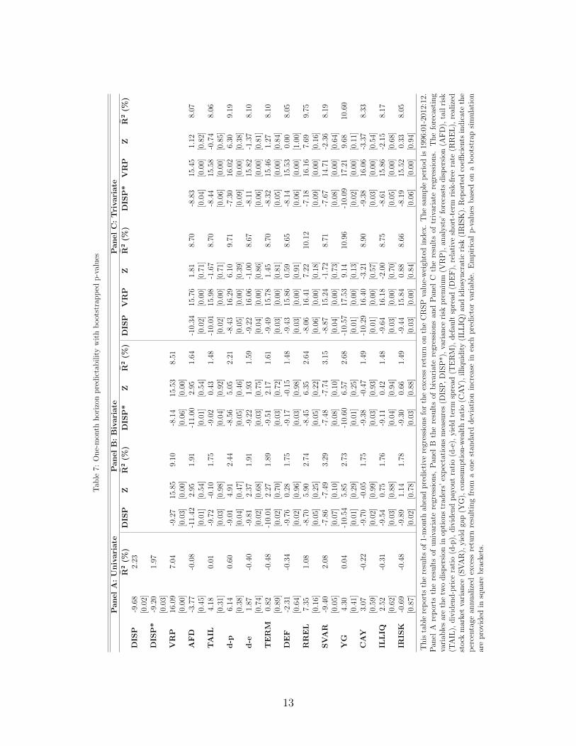
Tab

le7:

One-

mon

thhor

izon

pre

dic

tabilit

yw

ith

boot

stra

pp

edp-v

alues

PanelA:Univariate

PanelB:Bivariate

PanelC:Trivariate

R̃2(%

)DIS

PZ

R̃2(%

)DIS

P*

ZR̃

2(%

)DIS

PVRP

ZR̃

2(%

)DIS

P*

VRP

ZR̃

2(%

)DIS

P-9

.68

2.23

[0.0

2]DIS

P*

-9.2

01.

97[0

.03]

VRP

16.0

97.

04-9

.27

15.8

59.

10-8

.14

15.5

38.

51[0

.00]

[0.0

3][0

.00]

[0.0

6][0

.00]

AFD

-3.7

7-0

.08

-11.

422.

951.

91-1

1.00

2.95

1.64

-10.

3415

.76

1.81

8.70

-8.8

315

.45

1.12

8.07

[0.4

5][0

.01]

[0.5

4][0

.01]

[0.5

4][0

.02]

[0.0

0][0

.71]

[0.0

4][0

.00]

[0.8

2]TAIL

4.18

0.01

-9.7

2-0

.10

1.75

-9.0

20.

431.

48-1

0.01

15.9

8-1

.67

8.70

-8.4

415

.58

-0.7

48.

06[0

.31]

[0.0

3][0

.98]

[0.0

4][0

.92]

[0.0

2][0

.00]

[0.7

1][0

.06]

[0.0

0][0

.85]

d-p

6.14

0.60

-9.0

14.

912.

44-8

.56

5.05

2.21

-8.4

316

.29

6.10

9.71

-7.3

016

.02

6.30

9.19

[0.3

8][0

.04]

[0.4

7][0

.05]

[0.4

6][0

.05]

[0.0

0][0

.39]

[0.0

9][0

.00]

[0.3

8]d-e

1.87

-0.4

0-9

.81

2.37

1.91

-9.2

21.

931.

59-9

.22

16.0

6-1

.00

8.67

-8.1

115

.82

-1.3

78.

10[0

.74]

[0.0

2][0

.68]

[0.0

3][0

.75]

[0.0

4][0

.00]

[0.8

6][0

.06]

[0.0

0][0

.81]

TERM

0.82

-0.4

8-1

0.01

2.27

1.89

-9.5

12.

171.

61-9

.49

15.7

81.

458.

70-8

.32

15.4

61.

278.

10[0

.89]

[0.0

2][0

.70]

[0.0

3][0

.72]

[0.0

3][0

.00]

[0.8

1][0

.05]

[0.0

0][0

.84]

DEF

-2.3

1-0

.34

-9.7

60.

281.

75-9

.17

-0.1

51.

48-9

.43

15.8

60.

598.

65-8

.14

15.5

30.

008.

05[0

.64]

[0.0

2][0

.96]

[0.0

3][0

.98]

[0.0

3][0

.00]

[0.9

1][0

.06]

[0.0

0][1

.00]

RREL

7.35

1.08

-8.7

05.

902.

74-8

.45

6.35

2.64

-8.0

616

.41

7.22

10.1

2-7

.18

16.1

67.

699.

75[0

.16]

[0.0

5][0

.25]

[0.0

5][0

.22]

[0.0

6][0

.00]

[0.1

8][0

.09]

[0.0

0][0

.16]

SVAR

-9.4

02.

08-7

.86

-7.4

93.

29-7

.48

-7.7

43.

15-8

.87

15.2

4-1

.72

8.71

-7.6

714

.71

-2.3

68.

19[0

.05]

[0.0

7][0

.10]

[0.0

8][0

.10]

[0.0

4][0

.00]

[0.7

3][0

.08]

[0.0

0][0

.64]

YG

4.30

0.04

-10.

545.

852.

73-1

0.60

6.57

2.68

-10.

5717

.53

9.14

10.9

6-1

0.09

17.2

19.

6810

.60

[0.4

1][0

.01]

[0.2

9][0

.01]

[0.2

5][0

.01]

[0.0

0][0

.13]

[0.0

2][0

.00]

[0.1

1]CAY

3.07

-0.2

2-9

.70

-0.0

51.

75-9

.38

-0.4

71.

49-1

0.29

16.4

0-3

.21

8.90

-9.3

816

.06

-3.3

78.

33[0

.59]

[0.0

2][0

.99]

[0.0

3][0

.93]

[0.0

1][0

.00]

[0.5

7][0

.03]

[0.0

0][0

.54]

ILLIQ

2.52

-0.3

1-9

.54

0.75

1.76

-9.1

10.

421.

48-9

.64

16.1

8-2

.00

8.75

-8.6

115

.86

-2.1

58.

17[0

.62]

[0.0

3][0

.88]

[0.0

4][0

.94]

[0.0

3][0

.00]

[0.7

0][0

.05]

[0.0

0][0

.68]

IRIS

K-0

.69

-0.4

8-9

.89

1.14

1.78

-9.3

00.

661.

49-9

.44

15.8

40.

888.

66-8

.19

15.5

20.

338.

05[0

.87]

[0.0

2][0

.78]

[0.0

3][0

.88]

[0.0

3][0

.00]

[0.8

4][0

.06]

[0.0

0][0

.94]

This

table

rep

orts

the

resu

lts

of1-

mon

thah

ead

pre

dic

tive

regr

essi

ons

for

the

exce

ssre

turn

onth

eC

RSP

valu

e-w

eigh

ted

index

.T

he

sam

ple

per

iod

is19

96:0

1-20

12:1

2.P

anel

Are

por

tsth

ere

sult

sof

univ

aria

tere

gres

sion

s,P

anel

Bth

ere

sult

sof

biv

aria

tere

gres

sion

san

dP

anel

Cth

ere

sult

sof

triv

aria

tere

gres

sion

s.T

he

fore

cast

ing

vari

able

sar

eth

etw

odis

per

sion

inop

tion

str

ader

s’ex

pec

tati

ons

mea

sure

s(D

ISP

,D

ISP

*),

vari

ance

risk

pre

miu

m(V

RP

),an

alyst

s’fo

reca

sts

dis

per

sion

(AF

D),

tail

risk

(TA

IL),

div

iden

d-p

rice

rati

o(d

-p),

div

iden

dpay

out

rati

o(d

-e),

yie

ldte

rmsp

read

(TE

RM

),def

ault

spre

ad(D

EF

),re

lati

vesh

ort-

term

risk

-fre

era

te(R

RE

L),

real

ized

stock

mar

ket

vari

ance

(SV

AR

),yie

ldga

p(Y

G),

consu

mpti

on-w

ealt

hra

tio

(CA

Y),

illiquid

ity

(IL

LIQ

)an

did

iosy

ncr

atic

risk

(IR

ISK

).R

epor

ted

coeffi

cien

tsin

dic

ate

the

per

centa

gean

nual

ized

exce

ssre

turn

resu

ltin

gfr

oma

one

stan

dar

ddev

iati

onin

crea

sein

each

pre

dic

tor

vari

able

.E

mpir

ical

p-v

alues

bas

edon

ab

oot

stra

psi

mula

tion

are

pro

vid

edin

squar

ebra

cket

s.

13

Table 8: Univariate long-horizon predictability with bootstrapped p-values

h=3 h=6 h=12 h=24

R̃2 (%) R̃2 (%) R̃2 (%) R̃2 (%)DISP -7.39 3.61 -5.47 3.54 -6.67 10.89 -5.19 12.72

[0.01] [0.01] [0.00] [0.00]DISP* -7.10 3.30 -5.10 3.00 -6.65 10.80 -5.20 12.74

[0.01] [0.01] [0.00] [0.00]VRP 13.05 12.32 8.34 8.90 3.94 3.46 2.90 3.58

[0.00] [0.00] [0.01] [0.02]AFD -4.49 1.02 -5.10 3.01 -5.78 8.04 -5.02 11.88

[0.14] [0.04] [0.00] [0.00]TAIL -1.21 -0.39 -1.48 -0.22 2.22 0.74 3.58 5.75

[0.64] [0.45] [0.12] [0.00]d-p 6.70 2.88 7.67 7.44 8.23 16.84 8.32 33.56

[0.13] [0.03] [0.00] [0.00]d-e 3.42 0.38 4.38 2.09 4.28 4.17 6.10 17.79

[0.37] [0.16] [0.08] [0.00]TERM 1.01 -0.43 1.82 -0.06 4.03 3.64 7.55 27.54

[0.78] [0.51] [0.10] [0.00]DEF -0.27 -0.50 2.07 0.07 3.30 2.27 4.22 8.22

[0.93] [0.37] [0.08] [0.01]RREL 7.63 3.89 7.65 7.39 6.53 10.41 -0.58 -0.40

[0.03] [0.01] [0.00] [0.67]SVAR -4.88 1.29 0.49 -0.48 2.37 0.92 2.48 2.48

[0.10] [0.80] [0.14] [0.06]YG 3.79 0.58 2.96 0.67 2.28 0.81 0.77 -0.27

[0.25] [0.16] [0.12] [0.52]CAY 3.41 0.37 3.17 0.85 3.24 2.17 3.52 5.56

[0.34] [0.25] [0.13] [0.04]ILLIQ 2.57 -0.01 1.46 -0.22 0.95 -0.29 0.07 -0.56

[0.42] [0.55] [0.59] [0.95]IRISK -1.63 -0.30 1.59 -0.17 1.40 -0.02 1.22 0.17

[0.54] [0.43] [0.37] [0.30]

This table reports the results of 3-, 6-, 12- and 24-month ahead univariate pre-dictive regressions for the excess return on the CRSP value-weighted index. Thesample period is 1996:01-2012:12. The forecasting variables are the two dispersionin options traders’ expectations measures (DISP, DISP*), variance risk premium(VRP), analysts’ forecasts dispersion (AFD), tail risk (TAIL), dividend-price ra-tio (d-p), dividend payout ratio (d-e), yield term spread (TERM), default spread(DEF), relative short-term risk-free rate (RREL), realized stock market variance(SVAR), yield gap (YG), consumption-wealth ratio (CAY), illiquidity (ILLIQ) andidiosyncratic risk (IRISK). Reported coefficients indicate the percentage annualizedexcess return resulting from a one standard deviation increase in each predictor vari-able. Empirical p-values based on a bootstrap simulation are provided in squarebrackets.

14

Tab

le9:

Tri

vari

ate

long-

hor

izon

pre

dic

tabilit

yw

ith

boot

stra

pp

edp-v

alues

PanelA:3-m

onth

horizo

nPanelB:6-m

onth

horizo

n

DIS

PVRP

ZR̃

2(%

)DIS

P*

VRP

ZR̃

2(%

)DIS

PVRP

ZR̃

2(%

)DIS

P*

VRP

ZR̃

2(%

)AFD

-6.3

212

.92

-1.2

315

.28

-5.1

112

.76

-1.8

214

.53

-3.1

48.

40-3

.58

12.8

7-1

.92

8.38

-4.2

612

.31

[0.0

2][0

.00]

[0.6

8][0

.05]

[0.0

0][0

.54]

[0.1

2][0

.00]

[0.1

3][0

.34]

[0.0

0][0

.08]

TAIL

-10.

1013

.42

-6.9

318

.12

-8.7

513

.01

-6.0

816

.68

-7.9

48.

72-5

.93

15.5

2-6

.82

8.39

-5.2

613

.82

[0.0

0][0

.00]

[0.0

1][0

.00]

[0.0

0][0

.03]

[0.0

0][0

.00]

[0.0

1][0

.00]

[0.0

0][0

.01]

d-p

-6.0

913

.32

6.72

18.5

6-5

.30

13.1

36.

8717

.88

-4.1

58.

727.

6219

.47

-3.4

68.

597.

7418

.76

[0.0

3][0

.00]

[0.1

3][0

.05]

[0.0

0][0

.12]

[0.0

4][0

.00]

[0.0

3][0

.09]

[0.0

0][0

.03]

d-e

-7.1

212

.61

1.18

15.3

1-6

.25

12.4

30.

9014

.43

-5.4

57.

563.

1313

.01

-4.6

37.

432.

9011

.88

[0.0

1][0

.00]

[0.7

5][0

.02]

[0.0

0][0

.81]

[0.0

1][0

.00]

[0.3

0][0

.02]

[0.0

0][0

.33]

TERM

-7.2

612

.78

1.45

15.3

6-6

.42

12.5

41.

3214

.50

-5.5

98.

092.

2412

.41

-4.8

67.

912.

1311

.38

[0.0

1][0

.00]

[0.7

1][0

.02]

[0.0

0][0

.73]

[0.0

1][0

.00]

[0.4

4][0

.02]

[0.0

0][0

.47]

DEF

-7.5

912

.90

2.06

15.5

1-6

.61

12.6

31.

6014

.56

-6.2

98.

273.

9113

.68

-5.3

68.

063.

4912

.35

[0.0

1][0

.00]

[0.5

2][0

.01]

[0.0

0][0

.62]

[0.0

0][0

.00]

[0.1

3][0

.01]

[0.0

0][0

.17]

RREL

-5.7

513

.45

7.65

19.5

1-5

.23

13.2

77.

9719

.11

-3.9

68.

797.

6119

.38

-3.5

58.

677.

8418

.98

[0.0

4][0

.00]

[0.0

4][0

.05]

[0.0

0][0

.03]

[0.0

5][0

.00]

[0.0

1][0

.08]

[0.0

0][0

.01]

SVAR

-7.4

913

.54

1.89

15.4

3-6

.50

13.0

91.

3414

.49

-6.6

810

.35

5.94

15.6

4-5

.66

9.95

5.43

14.0

9[0

.01]

[0.0

0][0

.54]

[0.0

2][0

.00]

[0.6

7][0

.00]

[0.0

0][0

.02]

[0.0

1][0

.00]

[0.0

3]YG

-8.1

114

.23

7.59

19.3

6-7

.84

13.9

98.

0418

.93

-6.0

19.

205.

4915

.64

-5.6

89.

025.

7915

.02

[0.0

0][0

.00]

[0.0

5][0

.00]

[0.0

0][0

.04]

[0.0

0][0

.00]

[0.0

3][0

.01]

[0.0

0][0

.03]

CAY

-7.4

713

.08

-1.3

315

.33

-6.7

612

.84

-1.4

314

.50

-5.2

58.

200.

0411

.74

-4.5

38.

030.

0510

.78

[0.0

1][0

.00]

[0.7

1][0

.01]

[0.0

0][0

.68]

[0.0

1][0

.00]

[0.9

9][0

.03]

[0.0

0][0

.99]

ILLIQ

-7.2

113

.01

-0.9

315

.27

-6.4

612

.77

-1.0

414

.45

-5.4

28.

35-0

.89

11.8

4-4

.75

8.18

-0.9

510

.89

[0.0

1][0

.00]

[0.7

7][0

.02]

[0.0

0][0

.75]

[0.0

1][0

.00]

[0.7

1][0

.02]

[0.0

0][0

.69]

IRIS

K-6

.96

12.8

7-0

.44

15.2

2-6

.11

12.6

3-0

.85

14.4

3-5

.77

8.18

2.64

12.6

5-4

.91

7.99

2.29

11.4

7[0

.01]

[0.0

0][0

.87]

[0.0

3][0

.00]

[0.7

6][0

.01]

[0.0

0][0

.23]

[0.0

1][0

.00]

[0.2

9]

(to

be

conti

nued

)

15

(con

tinued

)

PanelC:12-m

onth

horizo

nPanelD:24-m

onth

horizo

n

DIS

PVRP

ZR̃

2(%

)DIS

P*

VRP

ZR̃

2(%

)DIS

PVRP

ZR̃

2(%

)DIS

P*

VRP

ZR̃

2(%

)AFD

-4.7

34.

03-3

.33

15.6

8-4

.42

3.83

-3.4

115

.03

-3.1

53.

08-3

.53

19.7

4-2

.97

2.96

-3.6

119

.29

[0.0

0][0

.01]

[0.0

6][0

.00]

[0.0

2][0

.05]

[0.0

1][0

.02]

[0.0

1][0

.01]

[0.0

2][0

.01]

TAIL

-7.4

63.

97-1

.78

14.3

4-7

.13

3.62

-1.5

013

.52

-4.5

52.

641.

2116

.04

-4.4

02.

421.

3615

.62

[0.0

0][0

.02]

[0.2

4][0

.00]

[0.0

3][0

.31]

[0.0

0][0

.03]

[0.2

8][0

.00]

[0.0

4][0

.23]

d-p

-5.2

14.

307.

5327

.87

-4.9

94.

077.

5527

.28

-3.3

33.

277.

7643

.82

-3.1

53.

137.

7843

.25

[0.0

0][0

.01]

[0.0

1][0

.00]

[0.0

2][0

.01]

[0.0

0][0

.01]

[0.0

0][0

.01]

[0.0

1][0

.00]

d-e

-7.0

02.

934.

2918

.26

-6.6

62.

684.

0517

.12

-6.0

21.

336.

6135

.89

-5.7

61.

116.

4534

.41

[0.0

0][0

.06]

[0.0

8][0

.00]

[0.0

9][0

.09]

[0.0

0][0

.25]

[0.0

0][0

.00]

[0.3

4][0

.00]

TERM

-7.2

53.

574.

8319

.64

-7.0

63.

254.

7918

.90

-6.0

12.

168.

0647

.31

-5.7

11.

917.

9045

.59

[0.0

0][0

.03]

[0.0

6][0

.00]

[0.0

5][0

.06]

[0.0

0][0

.07]

[0.0

0][0

.00]

[0.1

1][0

.00]

DEF

-7.9

53.

905.

3820

.74

-7.5

23.

555.

0219

.29

-6.5

82.

865.

9331

.93

-6.2

42.

585.

6630

.10

[0.0

0][0

.02]

[0.0

1][0

.00]

[0.0

3][0

.02]

[0.0

0][0

.02]

[0.0

0][0

.00]

[0.0

4][0

.00]

RREL

-5.4

94.

255.

7822

.03

-5.5

04.

016.

0122

.15

-5.4

22.

63-1

.50

16.5

5-5

.22

2.41

-1.2

615

.65

[0.0

0][0

.01]

[0.0

1][0

.00]

[0.0

1][0

.01]

[0.0

0][0

.03]

[0.2

9][0

.00]

[0.0

5][0

.37]

SVAR

-8.5

66.

427.

1424

.16

-8.0

75.

906.

7122

.45

-6.7

14.

946.

1230

.38

-6.4

14.

555.

8628

.75

[0.0

0][0

.00]

[0.0

0][0

.00]

[0.0

0][0

.00]

[0.0

0][0

.00]

[0.0

0][0

.00]

[0.0

0][0

.00]

YG

-6.7

54.

473.

4516

.69

-6.7

84.

223.

8016

.65

-5.0

12.

970.

9815

.93

-4.9

32.

781.

1715

.54

[0.0

0][0

.01]

[0.0

5][0

.00]

[0.0

1][0

.03]

[0.0

0][0

.02]

[0.4

5][0

.00]

[0.0

2][0

.36]

CAY

-6.4

13.

710.

6313

.81

-6.3

03.

480.

3313

.09

-4.6

12.

451.

7716

.88

-4.4

82.

261.

6516

.07

[0.0

0][0

.02]

[0.7

6][0

.00]

[0.0

3][0

.87]

[0.0

0][0

.04]

[0.2

4][0

.00]

[0.0

6][0

.28]

ILLIQ

-6.6

83.

92-0

.60

13.8

1-6

.55

3.65

-0.8

113

.23

-5.1

92.

89-0

.90

15.8

7-5

.11

2.67

-0.9

915

.35

[0.0

0][0

.02]

[0.7

4][0

.00]

[0.0

3][0

.65]

[0.0

0][0

.02]

[0.5

1][0

.00]

[0.0

3][0

.46]

IRIS

K-7

.33

3.80

3.11

16.0

9-6

.99

3.48

2.81

15.0

3-5

.85

2.72

2.77

19.0

3-5

.65

2.46

2.60

18.0

6[0

.00]

[0.0

2][0

.08]

[0.0

0][0

.03]

[0.1

0][0

.00]

[0.0

3][0

.04]

[0.0

0][0

.05]

[0.0

5]

This

table

rep

orts

the

resu

lts

of3-

(Pan

elA

),6-

(Pan

elB

),12

-(P

anel

C)

and

24-m

onth

(Pan

elD

)ah

ead

triv

aria

tepre

dic

tive

regr

essi

ons

for

the

exce

ssre

turn

onth

eC

RSP

valu

e-w

eigh

ted

index

.T

he

sam

ple

per

iod

is19

96:0

1-20

12:1

2.T

he

fore

cast

ing

vari

able

sar

eth

etw

odis

per

sion

inop

tion

str

ader

s’ex

pec

tati

ons

mea

sure

s(D

ISP

,D

ISP

*),

vari

ance

risk

pre

miu

m(V

RP

),an

alyst

s’fo

reca

sts

dis

per

sion

(AF

D),

tail

risk

(TA

IL),

div

iden

d-p

rice

rati

o(d

-p),

div

iden

dpay

out

rati

o(d

-e),

yie

ldte

rmsp

read

(TE

RM

),def

ault

spre

ad(D

EF

),re

lati

vesh

ort-

term

risk

-fre

era

te(R

RE

L),

real

ized

stock

mar

ket

vari

ance

(SV

AR

),yie

ldga

p(Y

G),

consu

mpti

on-w

ealt

hra

tio

(CA

Y),

illiquid

ity

(IL

LIQ

)an

did

iosy

ncr

atic

risk

(IR

ISK

).R

epor

ted

coeffi

cien

tsin

dic

ate

the

per

centa

gean

nual

ized

exce

ssre

turn

resu

ltin

gfr

oma

one

stan

dar

ddev

iati

onin

crea

sein

each

pre

dic

tor

vari

able

.E

mpir

ical

p-v

alues

bas

edon

ab

oot

stra

psi

mula

tion

are

pro

vid

edin

squar

ebra

cket

s.

16

Table 10: ENC-NEW test for out-of-sample predictability

h=1 h=3 h=6DISP 5.25** 6.16** 5.16**DISP* 5.04** 5.99** 4.76**VRP 11.27** 22.44** 14.59**AFD 0.59 2.43** 2.48**TAIL -0.36 -2.89 -4.72d-p 0.88 0.59 3.72**d-e -0.63 -8.54 -17.59TERM -0.73 -4.85 -9.07DEF 2.46** 0.58 -8.17RREL 0.32 0.38 -1.91SVAR 1.97* -5.83 -3.51YG 4.68** 9.62** 9.12**CAY 0.70 1.39 0.44ILLIQ 2.88** 4.88** -2.31IRISK -2.69 -3.24 -3.22

This table reports the results of the ENC-NEW encom-passing test of Clark and McCracken (2001). The totalsample period is 1996:01-2012:12 and the forecasting pe-riod begins in 2000:01. The forecasting variables are thetwo dispersion in options traders’ expectations measures(DISP, DISP*), variance risk premium (VRP), analysts’forecasts dispersion (AFD), tail risk (TAIL), dividend-priceratio (d-p), dividend payout ratio (d-e), yield term spread(TERM), default spread (DEF), relative short-term risk-free rate (RREL), realized stock market variance (SVAR),yield gap (YG), consumption-wealth ratio (CAY), illiquid-ity (ILLIQ) and idiosyncratic risk (IRISK). ** and * denotesignificance at the 5% and 10% levels.

17

Table 11: Myopic portfolio rotation strategies

Mean (%) St. Dev. (%) Sharpe ∆CER (%) MDD (%) Long (%)Panel A: Portfolio Strategies for DISP and DISP*

Buy & Hold 4.76 25.15 0.19 -67.86

DISPSize 6.26 24.62 0.25 1.90 -67.48 100.00B/M 2.15 19.63 0.11 1.11 -62.25 100.00Mom 3.72 19.67 0.19 2.66 -50.47 100.00Industry 3.53 22.70 0.16 0.54 -62.41 100.00LT Reversal 8.68 22.00 0.39 6.16 -49.64 100.00ST Reversal 6.27 19.52 0.32 5.29 -54.18 100.00Pooled 8.11 24.93 0.33 3.52 -51.61 100.00

DISP*Size 7.51 24.15 0.31 3.50 -61.28 100.00B/M 1.23 18.89 0.07 0.62 -60.19 100.00Mom 2.58 19.50 0.13 1.62 -51.54 100.00Industry 3.24 21.98 0.15 0.73 -63.31 100.00LT Reversal 7.44 22.37 0.33 4.67 -52.28 100.00ST Reversal 6.81 19.40 0.35 5.90 -47.21 100.00Pooled 8.12 23.82 0.34 4.34 -43.69 100.00

Panel B: Pooled Portfolio Strategies for Alternative PredictorsVRP 18.51 28.87 0.64 10.74 -57.34 100.00AFD 7.58 25.88 0.29 2.27 -50.53 100.00TAIL 1.54 25.81 0.06 -3.72 -73.21 100.00d-p 3.38 33.60 0.10 -8.83 -76.54 100.00d-e 8.11 30.79 0.26 -1.38 -75.11 100.00TERM 8.07 29.57 0.27 -0.31 -64.15 100.00DEF 1.05 28.85 0.04 -6.70 -76.33 100.00RREL -3.08 27.85 -0.11 -9.98 -82.69 100.00SVAR 1.25 29.00 0.04 -6.63 -68.71 100.00YG 4.22 29.39 0.14 -4.00 -72.34 100.00CAY 2.15 24.39 0.09 -2.04 -68.03 100.00ILLIQ 5.15 25.85 0.20 -0.13 -60.14 100.00IRISK 3.39 31.94 0.11 -7.18 -78.38 100.00

This table reports the results of portfolio rotation strategies based on the 1-month ahead out-of-sample predictabil-ity for the excess stock portfolio returns. The total sample period is 1996:01-2012:12 and the forecasting periodbegins in 2000:01. The forecasting variables are the two dispersion in options traders’ expectations measures (DISP,DISP*), variance risk premium (VRP), analysts’ forecasts dispersion (AFD), tail risk (TAIL), dividend-price ratio(d-p), dividend payout ratio (d-e), yield term spread (TERM), default spread (DEF), relative short-term risk-freerate (RREL), realized stock market variance (SVAR), yield gap (YG), consumption-wealth ratio (CAY), illiquidity(ILLIQ) and idiosyncratic risk (IRISK). Buy & Hold refers to a passive strategy that takes a long position on themarket portfolio. Mean denotes the average return, St. Dev. denotes the standard deviation of returns, Sharpestands for the Sharpe ratio, ∆CER is the certainty equivalent return in excess of the buy-hold strategy, MDDstands for the maximum drawdown and Long is the percentage of months that the strategy takes a long positionon the two winner portfolios. All measures of performance apart from MDD are in annualized terms. The rotationstrategies use decile portfolios sorted on size (Size), book-market ratio (B/M), momentum (Mom), industry (Indus-try), long-term reversal (LT Reversal) and short-term reversal (ST Reversal). Pooled refers to a rotation strategythat uses all 60 portfolios. Panel A shows the results of the rotation strategies based on the forecasting performanceof the dispersion in options’ traders expectations, while Panel B shows the results of the rotation strategies usingall 60 portfolios based on the forecasting performance of the alternative predictors.

18

Table 12: Portfolio rotation strategies with alternative weights

Mean (%) St. Dev. (%) Sharpe ∆CER (%) MDD (%) Long (%)Panel A: Portfolio Strategies for DISP and DISP*

Buy & Hold 4.40 21.79 0.20 -61.95

DISPSize 9.86 18.94 0.52 7.20 -36.62 76.92B/M 2.72 16.89 0.16 1.16 -48.50 87.18Mom 5.28 17.10 0.31 3.62 -42.05 86.54Industry 3.87 20.44 0.19 0.33 -58.99 100.00LT Reversal 8.33 20.30 0.41 4.87 -44.55 92.95ST Reversal 7.83 16.71 0.47 6.36 -44.79 84.62Pooled 7.94 22.24 0.36 3.23 -46.10 100.00

DISP*Size 8.96 19.02 0.47 6.26 -34.24 75.64B/M 0.49 16.51 0.03 -0.88 -49.52 86.54Mom 3.78 16.89 0.22 2.21 -40.03 83.97Industry 3.92 19.83 0.20 0.74 -58.71 100.00LT Reversal 6.88 20.71 0.33 3.16 -46.98 93.59ST Reversal 8.39 16.39 0.51 7.08 -30.45 82.69Pooled 8.02 21.39 0.37 3.87 -41.55 100.00

Panel B: Pooled Portfolio Strategies for Alternative PredictorsVRP 15.66 26.29 0.60 8.01 -52.90 100.00AFD 7.22 23.49 0.31 3.68 -46.65 100.00TAIL 2.71 23.12 0.12 -2.59 -68.18 100.00d-p 3.73 30.45 0.12 -7.46 -73.44 100.00d-e 5.49 26.80 0.20 -2.56 -71.23 96.79TERM 7.83 26.78 0.29 -0.20 -60.31 100.00DEF 3.59 26.05 0.14 -3.87 -70.60 96.15RREL -1.20 25.11 -0.05 -7.93 -76.20 100.00SVAR 4.38 26.46 0.17 -3.41 -65.31 96.15YG 4.57 27.05 0.17 -3.69 -68.31 100.00CAY 2.98 21.93 0.14 0.50 -64.20 100.00ILLIQ 3.70 22.95 0.16 0.54 -53.06 96.15IRISK 3.67 28.70 0.13 -3.95 -73.01 100.00

This table reports the results of portfolio rotation strategies based on the 1-month ahead out-of-sample predictabil-ity for the excess stock portfolio returns. The total sample period is 1996:01-2012:12 and the forecasting periodbegins in 2000:01. The forecasting variables are the two dispersion in options traders’ expectations measures (DISP,DISP*), variance risk premium (VRP), analysts’ forecasts dispersion (AFD), tail risk (TAIL), dividend-price ratio(d-p), dividend payout ratio (d-e), yield term spread (TERM), default spread (DEF), relative short-term risk-freerate (RREL), realized stock market variance (SVAR), yield gap (YG), consumption-wealth ratio (CAY), illiquidity(ILLIQ) and idiosyncratic risk (IRISK). Buy & Hold refers to a passive strategy that takes a long position on themarket portfolio. Mean denotes the average return, St. Dev. denotes the standard deviation of returns, Sharpestands for the Sharpe ratio, ∆CER is the certainty equivalent return in excess of the buy-hold strategy, MDDstands for the maximum drawdown and Long is the percentage of months that the strategy takes a long positionon the two winner portfolios. All measures of performance apart from MDD are in annualized terms. The rotationstrategies use decile portfolios sorted on size (Size), book-market ratio (B/M), momentum (Mom), industry (Indus-try), long-term reversal (LT Reversal) and short-term reversal (ST Reversal). Pooled refers to a rotation strategythat uses all 60 portfolios. Panel A shows the results of the rotation strategies based on the forecasting performanceof the dispersion in options’ traders expectations, while Panel B shows the results of the rotation strategies usingall 60 portfolios based on the forecasting performance of the alternative predictors.

19

Table 13: In-sample predictability for alternative dispersion in options traders’ expectations measures

h=1 h=3 h=6 h=12 h=24

R̃2 (%) R̃2 (%) R̃2 (%) R̃2 (%) R̃2 (%)DISPI -10.17 2.52 -6.20 2.40 -4.67 2.44 -6.23 9.42 -4.54 9.58

(-2.51)** (-1.98)** (-1.75)* (-2.43)** (-2.01)**[-2.62]*** [-1.83]* [-1.53] [-2.12]** [-1.77]*

DISPII -8.40 1.56 -6.06 2.27 -4.46 2.17 -5.35 6.82 -3.60 5.82(-2.10)** (-2.05)** (-2.06)** (-2.08)** (-1.65)[-2.03]** [-1.97]** [-1.61] [-2.02]** [-1.47]

DISPIII -8.96 1.84 -6.81 2.99 -5.19 3.13 -6.06 8.89 -4.09 7.69(-2.16)** (-2.12)** (-2.20)** (-2.45)** (-1.94)*[-2.13]** [-2.14]** [-1.76]* [-2.18]** [-1.63]

DISPIV -8.85 1.79 -6.79 2.97 -4.96 2.82 -6.77 11.24 -4.83 10.93(-2.22)** (-2.36)** (-2.06)** (-2.89)*** (-2.02)**[-2.22]** [-2.14]** [-1.65]* [-2.36]** [-1.85]*

DISP*I -9.37 2.06 -6.11 2.31 -4.51 2.24 -6.33 9.75 -4.75 10.54

(-2.36)** (-2.19)** (-1.85)* (-2.74)*** (-2.14)**[-2.43]** [-1.90]* [-1.55] [-2.21]** [-1.91]*

DISP*II -10.44 2.68 -7.29 3.50 -4.70 2.48 -5.73 7.91 -3.61 5.86

(-2.47)** (-2.53)** (-2.37)** (-2.34)** (-1.72)*[-2.33]** [-2.32]** [-1.71]* [-2.11]** [-1.50]

DISP*III -10.10 2.48 -7.63 3.88 -4.82 2.63 -6.16 9.21 -3.85 6.75

(-2.44)** (-2.64)*** (-2.42)** (-2.59)** (-1.94)*[-2.38]** [-2.49]** [-1.75]* [-2.28]** [-1.63]

DISP*IV -8.50 1.61 -6.85 3.03 -4.42 2.13 -6.75 11.16 -4.72 10.43

(-2.17)** (-2.57)** (-1.98)** (-3.01)*** (-2.03)**[-2.16]** [-2.26]** [-1.58] [-2.42]** [-1.91]*

This table reports the results of 1-, 3-, 6-, 12- and 24-month ahead univariate predictive regressions for the excess return onthe CRSP value-weighted index. The sample period is 1996:01-2012:12. The forecasting variables are the two dispersion inexpectations measures created using options of all available moneynesses (DISPI and DISP*

I ), options expiring one monthahead (DISPII and DISP*

II), options with maturities between 10 and 60 calendar days (DISPIII and DISP*III) and options

with maturities between 10 and 180 calendar days (DISPIV and DISP*IV). Reported coefficients indicate the percentage

annualized excess return resulting from a one standard deviation increase in each predictor variable. Newey and West(1987) and Hodrick (1992) t-statistics with lag length equal to the forecasting horizon are reported in parentheses andsquare brackets respectively. ***, ** and * denote significance at the 1%, 5% and 10% levels.

20

Tab

le14

:O

ut-

of-s

ample

pre

dic

tabilit

yfo

ral

tern

ativ

edis

per

sion

inop

tion

str

ader

s’ex

pec

tati

ons

mea

sure

s

1-m

onth

horizo

n3-m

onth

horizo

n6-m

onth

horizo

nR

2 OS(%

)M

SE-F

MSE-A

dj

R2 COS(%

)R

2 OS(%

)M

SE-F

MSE-A

dj

R2 COS(%

)R

2 OS(%

)M

SE-F

MSE-A

dj

R2 COS(%

)DIS

PI

2.04

3.24

**1.

80**

3.26

1.34

2.06

**1.

023.

67-0

.96

-1.3

80.

685.

31DIS

PII

1.44

2.28

**1.

53*

2.34

2.00

3.11

**1.

223.

391.

472.

18**

1.20

5.43

DIS

PIII

1.59

2.52

**1.

55*

2.20

2.54

3.96

**1.

233.

891.

862.

77**

1.15

6.06

DIS

PIV

1.05

1.65

**1.

49*

2.37

2.65

4.13

**1.

44*

4.71

0.92

1.36

*1.

156.

88DIS

P* I

1.53

2.42

**1.

67**

2.74

1.52

2.35

**1.

193.

70-0

.63

-0.9

20.

855.

18DIS

P* II

2.59

4.16

**1.

82**

2.84

3.46

5.45

**1.

56*

3.83

2.21

3.30

**1.

45*

5.37

DIS

P* III

2.25

3.59

**1.

81**

2.67

3.84

6.07

**1.

65**

4.56

2.07

3.09

**1.

38*

5.91

DIS

P* IV

0.92

1.44

*1.

51*

2.38

2.72

4.25

**1.

58*

4.61

0.30

0.44

1.19

5.80

This

table

rep

orts

the

resu

lts

of1-

,3-

and

6-m

onth

ahea

dou

t-of

-sam

ple

pre

dic

tabilit

yfo

rth

eex

cess

retu

rnon

the

CR

SP

valu

e-w

eigh

ted

index

.T

he

tota

lsa

mple

per

iod

is19

96:0

1-20

12:1

2an

dth

efo

reca

stin

gp

erio

db

egin

sin

2000

:01.

The

fore

cast

ing

vari

able

sar

eth

etw

odis

per

sion

inex

pec

tati

ons

mea

sure

scr

eate

dusi

ng

opti

ons

ofal

lav

aila

ble

mon

eynes

ses

(DIS

PI

and

DIS

P* I),

opti

ons

expir

ing

one

mon

thah

ead

(DIS

PII

and

DIS

P* II

),op

tion

sw

ith

mat

uri

ties

bet

wee

n10

and

60ca

lendar

day

s(D

ISPIII

and

DIS

P* III)

and

opti

ons

wit

hm

aturi

ties

bet

wee

n10

and

180

cale

ndar

day

s(D

ISPIV

and

DIS

P* IV

).R

2 OS

isth

eou

t-of

-sam

ple

coeffi

cien

tof

det

erm

inat

ion,

MSE

-Fis

the

McC

rack

en(2

007)

F-s

tati

stic

,M

SE

-Adj

isth

eM

SE

-Adju

sted

stat

isti

cof

Cla

rkan

dW

est

(200

7)an

dR

2 COS

isth

eou

t-of

-sam

ple

coeffi

cien

tof

det

erm

inat

ion

when

the

out-

of-s

ample

pre

dic

tion

isre

stri

cted

tob

ep

osit

ive.

**an

d*

den

ote

sign

ifica

nce

atth

e5%

and

10%

leve

ls.

21