
Diskussionspapiere der DFG- Forschergruppe (Nr ...
41
Rechts-, Wirtschafts- und Verwaltungswissenschaftliche Sektion Fachbereich Wirtschaftswissenschaften Diskussionspapiere der DFG- Forschergruppe (Nr.: 3468269275): Heterogene Arbeit: Positive und Normative Aspekte der Qualifikationsstruktur der Arbeit Stefan Hupfeld Longevity and Redistribution in the German Pension System April 2006 Diskussionspapier Nr. 06/10 http://www.wiwi.uni-konstanz.de/forschergruppewiwi/
Transcript of Diskussionspapiere der DFG- Forschergruppe (Nr ...
Rechts-, Wirtschafts- und Verwaltungswissenschaftliche Sektion Fachbereich Wirtschaftswissenschaften
Diskussionspapiere der DFG-Forschergruppe (Nr.: 3468269275):
Heterogene Arbeit: Positive und Normative Aspekte der Qualifikationsstruktur der Arbeit Stefan Hupfeld Longevity and Redistribution in the German Pension System April 2006 Diskussionspapier Nr. 06/10 http://www.wiwi.uni-konstanz.de/forschergruppewiwi/

Diskussionspapier der Forschergruppe (Nr.: 3468269275) “Heterogene Arbeit: Positive und Normative Aspekte der Qualifikationsstruktur der Arbeit“
Nr. 06/10, April 2006
Longevity and Redistribution in the German Pension System
Stefan Hupfeld Universität Konstanz Fachbereich Wirtschaftswissenschaften Fach D136 78457 Konstanz Germany mail: [email protected]
phone: +49-7531-88-2534 fax +49-7531-88-4135
Zusammenfassung: Abstract: There are theoretical foundations which allow hypothesizing on a positive association of life expectancy or retirement age with income. If both cannot be falsified, the relationship of income and the internal rate of return of a public pension system is not straight forward. By application of a partially linear model to micro data from the German public pension system, it is found that neither life expectancy, nor retirement age is monotonously increasing in income, as measured in benefit claims. The relation of benefit claims and duration under the benefit spell (which determines the rate of return) depends on the set of covariates. Including pensions for disabled individuals, three out of four specifications exhibit a duration decreasing in benefit claims. JEL Klassifikation : H55, I12, H23 Schlüsselwörter : Public Pension System, Life Expectancy, Redistribution, Partially Linear Model Download/Reference : http://www.wiwi.uni-konstanz.de/forschergruppewiwi/
Longevity and Redistribution in the GermanPension System
Stefan Hupfeld∗
This Version: April 4, 2006
Abstract: There are theoretical foundations which allow hypothesizing
on a positive association of life expectancy or retirement age with income.
If both cannot be falsified, the relationship of income and the internal rate
of return of a public pension system is not straight forward. By appli-
cation of a partially linear model to micro data from the German public
pension system, it is found that neither life expectancy, nor retirement age
is monotonously increasing in income, as measured in benefit claims. The
relation of benefit claims and duration under the benefit spell (which de-
termines the rate of return) depends on the set of covariates. Including
pensions for disabled individuals, three out of four specifications exhibit a
duration decreasing in benefit claims.
Keywords: Public Pension System, Life Expectancy, Redistribution,
Partially Linear Model
JEL-Classification: H55, I12, H23
∗Department of Economics, Box D136, University of Konstanz, 78457 Konstanz, Germany,[email protected] gratefully acknowledge support by the German Research Foundation (DFG) under grant no. 454,"Heterogeneous Labor: Positive and Normative Aspects of the Skill Structure of Labor". The for-mer Federation of German Pension Insurance Institutes (VDR, now: Deutsche RentenversicherungBund) deserves thanks for producing and confiding the data set.I thank Friedrich Breyer, Mathias Kifmann, Winfried Pohlmeier, and Leo Kaas for helpful discus-sions and suggestions. All errors are my own.
1. Introduction
1. Introduction
There are good reasons to believe in the often corroborated positive relationship be-
tween income and life expectancy. The case of Germany is considered by Reil-Held
(2000), who basically compares different income quantiles. Additionally, there are the-
oretical foundations for such a phenomenon, among the earliest the model of health
capital, introduced by Grossman (1972). Such a monotonous relation would have
potentially unintented consequences for a public pension scheme organized as a pay-
as-you-go system, namely resulting in redistribution from poor to rich, as Diamond
(2003), pp. 87 shows. However, in the following essay it is shown that the mechanism
that links income and life expectancy is far more complex, at least for the participants
in a public pension system. The association between life expectancy, retirement age
and duration with collected benefit claims is estimated by a partially linear model,
taking endogeneity of the collected benefit claims regarding retirement age into ac-
count. Though stable relationships can be discovered, they are not of the kind that life
expectancy or retirement age is monotonously linked to benefit claims. Additionally,
there is no unique evidence for redistribution, since not life expectancy or retirement
age alone drives the rate of return from the pension system, but the duration under
the benefit spell. The latter is found to be either increasing or decreasing in collected
claims, depending of the specification of the econometric model.
Theory There are several strands of literature which derive second best properties of
a pension system and take individual heterogeneity into account. The first to be con-
sidered is Diamond (2003), who uses a framework of optimal taxation. The dimension
in which individuals may differ is (firstly) disutility of labor, which is not observable by
the social planner. The individual is free to choose whether to retire in the second or
third period within his three-period life1, and this decision depends on the individual
degree of disutility of labor and on the taxation on work in the second period, which
is implied by the pension system. Workers with a disutility of labor beyond a certain
threshold prefer to retire early, and by maximizing a utilitarian welfare function, this is
optimal and should actually be induced by taxing work in the second period. However,
those who prefer to retire later should benefit in two ways, namely by a higher wage
in the second period and by higher benefits in the third period. The result can be
interpreted as a tax system which is contingent on age. The second possible dimension
of heterogeneity is life expectancy, and the decision to be taken by the individuals is
the same as under heterogeneous disutility of labor. A fourth period2 is introduced,
and the probability of reaching the fourth period as a retiree is taken as a measure
of life expectancy. Assuming a negative relation between disutility of labor and life
expectancy, the welfare maximizing pension scheme is more complicated: Those with
1The model is reducible to two periods, as everybody will work in the first period.2Again, the model is reducible by one period.
1
1. Introduction
very high life expectancy will be able to take advantage of the pension scheme, be-
cause they can easily retire later, but benefit from a relatively low implicit taxation
of prolonged work. This relatively low implicit taxation of work in the second period
is necessary in order to provide incentives to work for those at the margin (meaning,
with an intermediary life expectancy). At the same time, those individuals with very
short life expectancy suffer from a relatively low rate of return, which is necessary for
exactly the same reason. Diamond (2003) shows that the unequal treatment that ben-
efits those with high life expectancy can be (partially) overcome by the introduction
of a private (and perfectly discriminating) annuity market, together with lump sum
payments from the public pension system.
A comparable approach in the framework of optimal taxation is taken by Cremer
and Pestieau (1996) and Cremer, Lozachmeur, and Pestieau (2004). The earlier con-
tribution starts right away with the assumption of two dimensions in which individuals
may differ, namely ability and risk (of incurring a loss), which are both unobservable.
Note that these dimensions can basically be transformed into the dimensions Diamond
(2003) assumes. However, the authors explicitly allow for different correlation struc-
tures. One correlation structure3 indicates that a partial social insurance system alone
will already reach the second best optimum. The later contribution uses the developed
framework and explicitly focusses on retirement. The two unobservable properties are
productivity and health, while the latter can be translated into the already known
disutility of labor. The authors find that early retirement for those "in bad health"
can be second best optimal (from a utilitarian point of view) and should actually be
induced by implicit taxation in the pension system.
In the above mentioned strands of literature, all heterogeneity regarding "health"
or similar concepts are taken to be exogenous. Grossman (1972) proposed a model
of health capital which can be augmented by (timely or costly) investments. The
benefits come directly in terms of utility, and indirectly in terms of better possibilities
to be productive. The time of death is also implicitly defined by the stock of health
capital, and under some assumptions (namely, stressing the investment property of
health capital), a positive relation between productivity and health (and therefore life
expectancy) can be derived.
Empirical Insights There is some literature on the different aspects of the present
analysis. For the case of life expectancy in Germany, Reil-Held (2000) finds a positive
relationship between income and life expectancy. Men in the lowest income quartile
must expect to be outlived by those in the highest quartile by six years, which is
estimated by Kaplan-Meier and Cox-estimation, even after controlling for several so-
cioeconomic factors. Exemplarily, Deaton and Paxson (2004) can show that income
reduces the risk of mortality in the United States.
3High ability ⇔ low disutility of labor is associated with high risk (of longevity) ⇔ high life ex-pectancy. This is equivalent to the correlation assumed by Diamond (2003).
2

1. Introduction
Mainly concerned with policy implications, Berkel and Börsch-Supan (2004) analyze
the impact of different socioeconomic variables on retirement behavior and find that
people with higher income or assets actually retire earlier after controlling for educa-
tion.4, which is not confirmed by Schils (2005), pp. 123, who finds a positive influence
of hourly wages on retirement age.5
As a potential link in the background, health (or health capital) ties economic ca-
pacity with life expectancy. In a more direct fashion, health status is a determinant
of retirement age. The evidence on a direct causal path from economic capacity to
health is mixed; Adams, Hurd, MacFadden, Merrill, and Ribeiro (2004) e. g. find a
health promoting causal relationship of wealth only for certain diseases, however, some
of which are found to drive mortality in a second step, such that a causal link between
wealth and mortality via health can be corroborated.
The German Public Pension System The pension system in Germany is today
organized as a pay-as-you-go system. Participation in (and therefore contribution to)
the German public pension system is mandatory for a large fraction of individuals, the
largest share of which is constituted by the dependent labor force. Contributions are
paid as a percentage of the relevant monthly gross income (if it is more than EUR 400).
In 2005, this fraction amounts to 19.5%, of which one half each is paid by the employer
and the employee. However, the relevant income is capped at EUR 5200 per month.
Other forms of employment are subject to more complex terms of participation in the
public pension system, e. g. self-employed can apply for participation.
Claims against the pension system are collected in points. Each point earned corre-
sponds to the contributions based on one average yearly income, which is now (2005, all
figures are for Western Germany) EUR 2415 per month. An individual earning exactly
the average income for 40 years will thus collect 40 points. In times of no regular em-
ployment, additional points can be earned through certain times of child care, ill health
or unemployment. This rather abstract claim is transformed into a monthly pension
benefit, depending on the general development of wages and employment. In the first
half of 2005, each point was worth EUR 26.13. The monthly benefit is then paid as
annuity to the beneficiary. Benefits are paid for several reasons, the most prominent is
the old-age pension, for which one is eligible at the age of 65. Contingent on a mini-
mum of 35 years of collecting claims, men can apply already at age 62 or 63 (depending
on their year of birth) for an old-age pension.6 They have to suffer from a discount,
namely 0.3% per month earlier than 65. Yet, although the discounts are intended to
be actuarially fair, on average they still provide incentives for early retirement, see
Börsch-Supan and Schnabel (1998). Under certain contingencies, benefits are paid to
4This phenomenon supports the conjecture of an income effect at the lower tail of the income distri-bution, see sections 5 and 6.
5To be precise, Schils (2005) finds that hourly wages decrease the hazard into retirement.6Different, but similar rules apply to women.
3

2. The Hypotheses
individuals incapable of working as well as to surviving spouses and orphans. The legal
basis for these rules can be found in SGB VI (German Social Security Code No. 6).
Organization of the Essay Section 2 will state the hypotheses explicitly. The data
set is introduced with some descriptive statistics in section 3. Section 4 then introduces
the estimation technique, namely the partially linear model, and covers related issues
such as bandwidth choice and confidence bands. The implementation of the suggested
methodology and the results are presented in section 5, and section 6 summarizes and
concludes.
2. The Hypotheses
The main concern of this work is on two hypotheses and a corollary. For ease of
exposition, they are clearly stated below.
Hypothesis 1 (Age) There is a positive relationship between socioeconomic status
and life expectancy among the participants of the German public pension system. The
socioeconomic status is measured by collected benefit claims (in points), whereas death
of the individual is directly observed. The positive association leads ceteris paribus to
redistribution to those with high benefit claims, since the internal rate of return of the
pension system increases with life expectancy.
Hypothesis 2 (Retirement Age) There is a positive relationship between socioeco-
nomic status and retirement age, which is due to the following reasons:
(i) Low income (and therefore low benefit claims) are associated with worse health.
Individuals who collected relatively few claims hereby are forced to retire earlier
due to their inability to work.
(ii) Relatively bad health (or low income) may be associated with high disutility of
labor. Individuals with low benefit claims deliberately choose to retire earlier.
(iii) Following hypothesis 1 (Age) and despite discounts for early retirement, individ-
uals with low benefit claims may choose to offset this disadvantage of shorter life
expectancy by retiring earlier.
Corollary (Duration) If both hypotheses 1 and 2 cannot be rejected, the aggregate
dependence of the duration under the pension benefit spell on socioeconomic status is
not clear, and therefore it is not clear how (or if) the internal rate of return from the
pension system is related to the collected benefit claims.
4

3. The Data
3. The Data
On the basis of the report of a commission7 installed by the German Federal Ministry of
Education and Research, the administrators of Germany’s social security system were
obliged to improve the cooperation among scientists and the various institutions of
social security. The German public pension system, represented by the former Federa-
tion of German Pension Insurance Institutes (VDR, now: Deutsche Rentenversicherung
Bund), began to publish their data in 2005. The data in use here is the collection of
pension discontinuations due to death of the beneficiary8, beginning in 1993 and ending
in 2003. The data set contains a 10% stratified sample (based on the federal states) of
all pensions that were discontinued, which adds to a total of 951,560 observations and
31 variables, described in table 1.
The data is not based on individuals, but on the pension, as the individual is not the
main subject of interest for the pension system. Sometimes both concepts coincide,
but accounting for benefits paid to widows and orphans, an individual may receive
more than one pension at a time. All these double payments are excluded. Pensions
paid to the insured himself cover both old-age pensions and disability pensions. The
latter are transferred to old-age pensions, once the beneficiary is eligible. Both are not
distinguishable in the data set. Additionally, the value of a benefit claim increases by
the potential payment to widows and orphans.
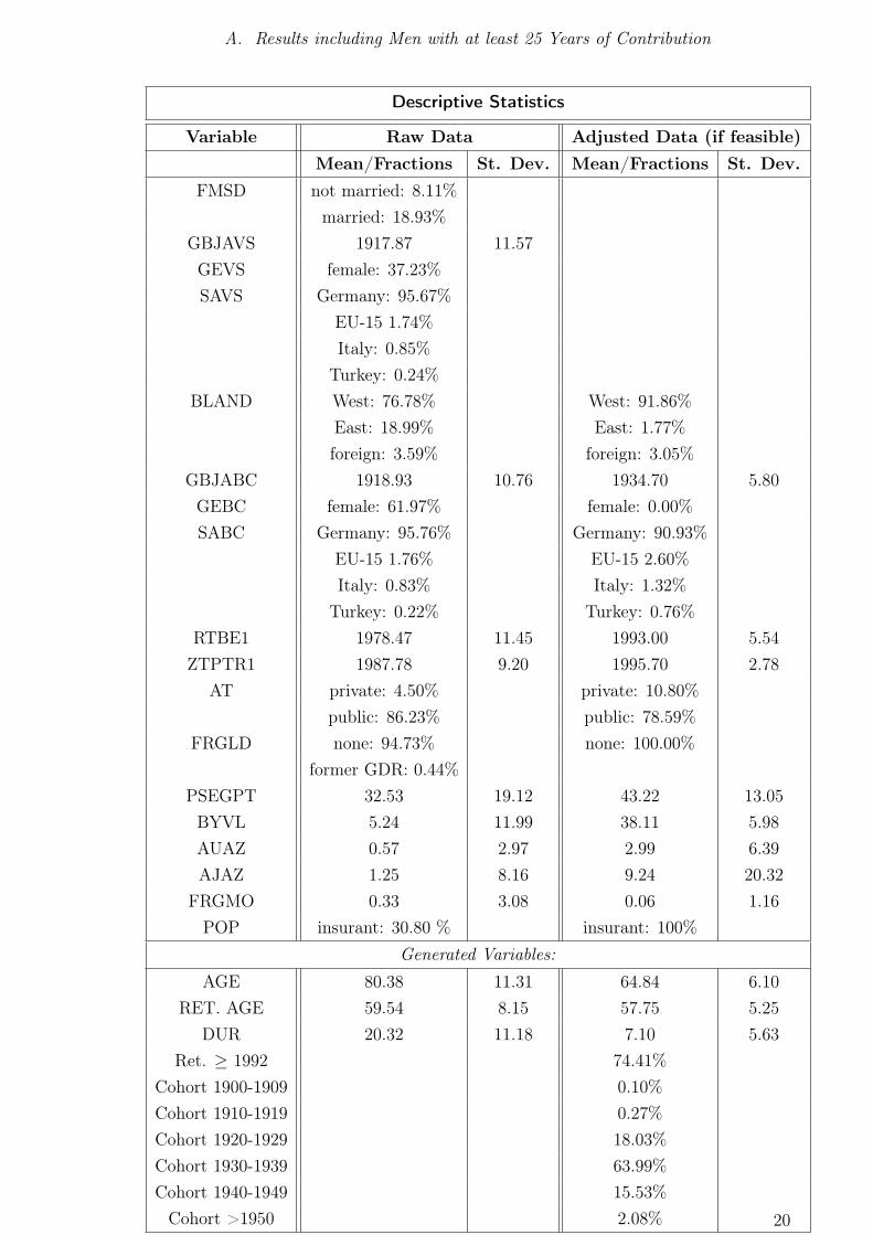
Descriptive Statistics In the following, some descriptive statistics of the data set
are presented. In table 2, mean and standard deviation are given for the variables of
interest, firstly for the whole (raw, but corrected for missing values) data, and secondly
for the adjusted data set as it is finally used for the estimation. At the bottom, the
descriptive statistics are given for variables which are not contained in the data set,
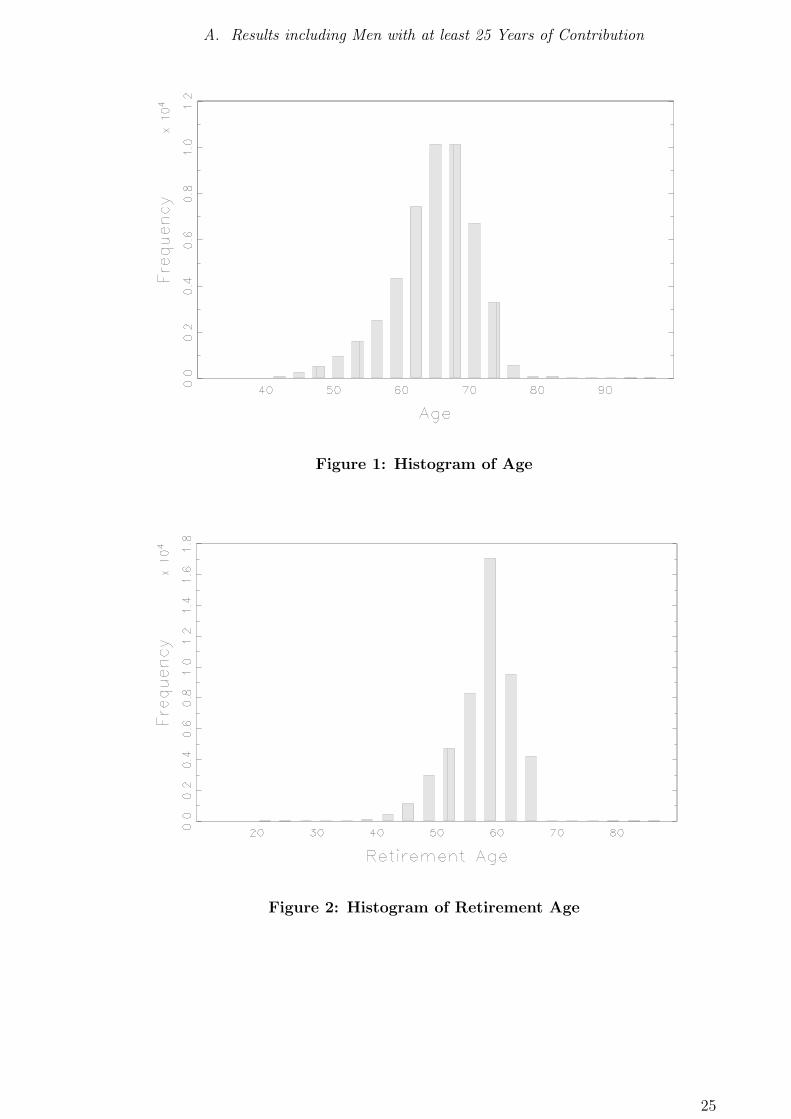
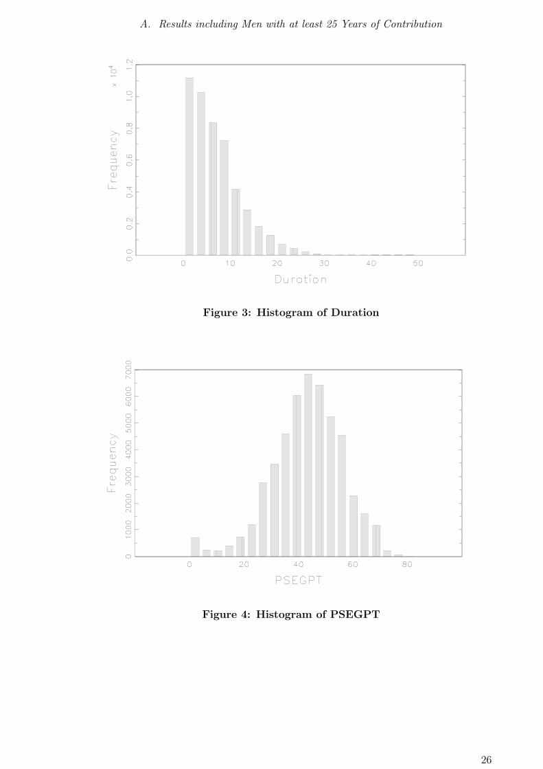
but which can be easily constructed. Histograms for age, retirement age, duration, and
collected claims (based on the adjusted data set) are presented in figures 1 to 4.
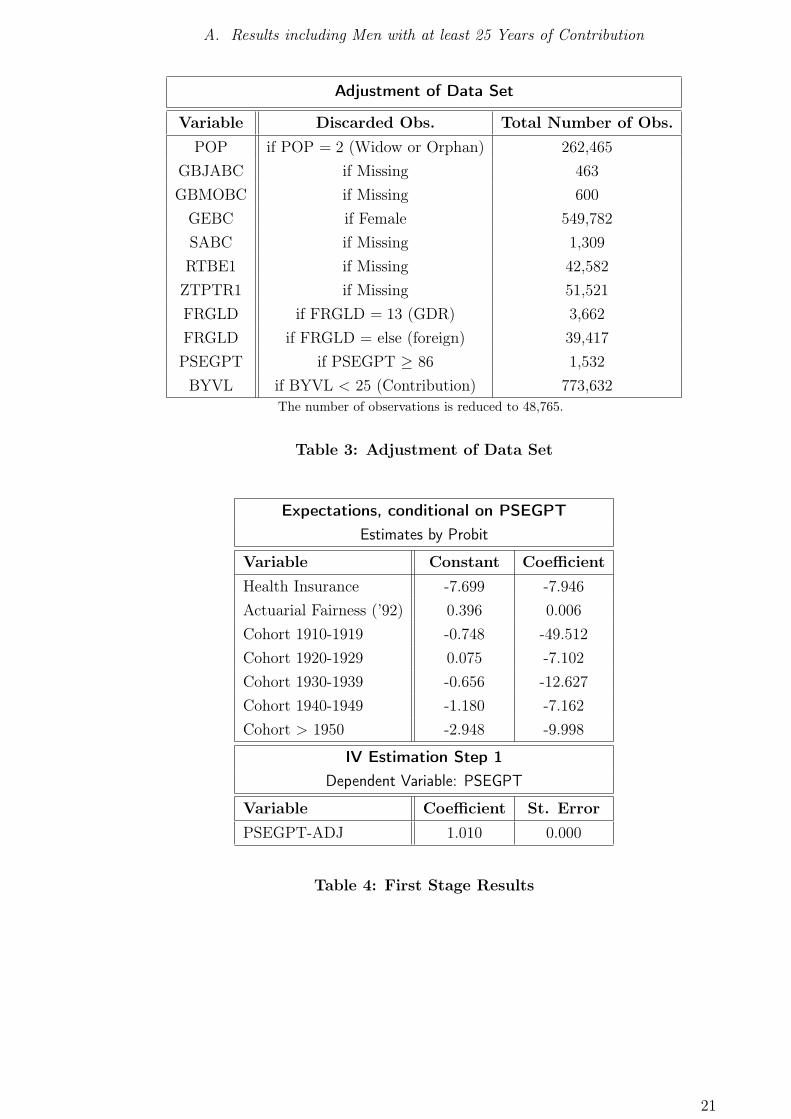
The raw data set is adjusted in the following way: Firstly, all observations containing
missing values concerning the date of birth and nationality are abandoned. Secondly,
only pensions that are based on own claims are considered, so especially all widower’s
or orphan’s pensions are discarded. There remain only those where the individual
that paid contributions coincides with the individual that benefits directly from the
pension. Finally, only male individuals who never worked in the former GDR are
considered. Female workers who retired between 1993 and 2003 seem to exhibit a
career pattern which is not comparable to the one of male workers. However, including
the few (roughly 10,000) female pensioners who worked at least 25 years does not
alter the later results substantially. People who worked in GDR and received benefit
7See: Kommission zur Verbesserung der informationellen Infrastruktur zwischen Wissenschaft undStatistik (2001).
8The "SUF Demographie Rentenwegfall 1993-2003 Versicherte, Witwer- und Witwen".
5
4. Methodology
claims after reunification are excluded, as the variance of wages in the former GDR
was relatively low and cannot be easily compared to wages paid in the former FRG.
All individuals who worked less than 25 years and contributed to the pension system
are excluded, as they do not represent the usual career pattern. However, the results
presented later are robust against the inclusion of individuals who worked less. The
adjusted data set contains 48,765 observations. Most of the dropped observations are
females and/or pensioners who worked less than 25 years, see table 3 for a detailed
description of the difference between raw and adjusted data.
4. Methodology
The major focus of this work is the relationship of two variables, namely age, retirement
age, or duration under the benefit spell as dependent variable and collected claims as
explanatory variable. Yet, there are more variables involved, which should be included
in the analysis, e.g. a dummy for the type of health insurance, and the months spent
in ill-health and unemployment.
Denote the respective dependent variables by the scalar yi (with i being the individ-
ual observation), the main explanatory variable (a scalar again) is denoted by zi, and
the additional control variables can be found in the vector xi, which is of dimension k.
In order to infer the nature of the relationship between zi and yi, it is convenient to
estimate this relation non-parametrically, circumventing an imposed linear or higher
polynomial structure. However, it is generally not convenient to estimate the influence
of all xi non-parametrically as well, due to the so-called curse of dimensionality. This
means that the requirement of observations increases exponentially with the number of
regressors, or put differently, the approximation error increases more than proportion-
ally if the number of observations is held constant, but the dimension of the regressor
matrix is increased.9 In order to inspect the combined influence of more than one vari-
able graphically, one is bound to two regressors that enter the model non-parametrically
anyhow.
Partially Linear Model Accounting for the trade-off between imposed structure and
the necessity of additional control variables, a partially linear model is applied. This
has the following form:
yi = f(zi) + x′
iβ + ǫi (1)
The function f is not known, only smoothness is assumed. The parameter vector β
is not known either. In order to approach an estimation technique, rewrite the partially
linear model in terms of expectations, conditional on zi:
9See e. g. Yatchew (2003), p. 17.
6

4. Methodology
E(yi|zi) = f(zi) + E(xi|zi)′β (2)
The conditional expectations are now estimated non-parametrically, e. g. by fitting
a local polynomial. Denote the estimates by
E(yi|zi) =: my(zi)
E(x1i|zi) =: mx1(zi)...
E(xki|zi) =: mxk(zi)
and
(mx1(zi) . . . mxk(zi))′ =: mx(zi). (3)
The partially linear model in terms of conditional expectations of equation 2 can
then be rewritten as
yi − my(zi) = [xi − mx(zi)]′β + ǫi, (4)
and β can be estimated by least squares. Denoting the estimate by β and using
equations 1, 2 and the definition 3, an estimate for f(zi) is finally obtained by
f(zi) = my(zi) − mx(zi)′β (5)
However, note that the elements of the partially linear model can only be identified
under two restrictions10, namely
E(ǫi|zi, xi) = 0 (6)
and the absence of a constant in the parametric regressor vector xi. The first con-
dition will be violated once yi and zi are endogenous variables. The latter is due to
the fact that f(z) is left unspecified, such that any constant term in xi can not be
distinguished from a shift of f(z).
10See e. g. Pagan and Ullah (1999), p. 198.
7
4. Methodology
Endogeneity Suppose that zi is endogenous in the sense that the identifying restric-
tion in equation 6 is violated. However, there exists a variable zi which does satisfy
this restriction and which is associated with the original zi by
zi = ziθ + ui. (7)
Under the further assumption of linearity of E(ǫi|zi, ui) = u′
iρ, the relationship among
the residuals can be expressed by
ǫi = u′
iρ + νi, (8)
where ǫi is the residual of the model in equation 1. The endogeneity-adjusted model
can then be written11 as
yi = f(zi) + u′
iρ + x′
iβ + νi (9)
and finally be estimated semi-parametrically as well, with ui entering the model as
additional parametric regressor. As ui is not directly observable, it has to be replaced
by an estimate, namely the residual of equation 7 estimated by least squares. The sig-
nificance of IV-residual in the final partially linear estimation will falsify the hypothesis
of exogeneity of the respective regressor.
Local Polynomial Estimation and Bandwidth Choice The non-parametric esti-
mates mx(zi) and my(zi) still desire choices to be taken that influence the shape of the
analyzed relation, namely
(i) The degree p of the local polynomial: The most prominent choices are p = 0
(which leads to the Nadaraya-Watson estimator) or p = 1. Consider the non-
parametric estimator my(z), for example12. The estimator minimizes one of the
following terms, depending on either p = 0 or p = 1 (the extension to polynomials
of higher order is straight forward):13
p = 0 : m(0)y (zi) = arg min
m(0)
n∑
i=1
(yi − m(0)
y (zi))2
K
(zi − z
h
)(10)
p = 1 : m(1)y (zi) = arg min
m(1),β
n∑
i=1
(yi − m(1)
y (zi) − (zi − z)β)2
K
(zi − z
h
)(11)
11See Yatchew (2003), pp. 87 and Blundell and Duncan (1998).12The following applies to the estimation of mx(z) as well.13Compare e. g. Pagan and Ullah (1999), pp. 93.
8
4. Methodology
The estimator m(·)y (z) therefore either fits a local constant or a local line around
xi, weighting the neighboring observations around xi with the kernel function
K(·). Note that (whenever applicable), the respective objective functions are
also minimized with respect to the local β. In the case of p = 1, the asymptotic
bias of the estimated function is zero, which is not the case under p = 0, compare
Mittelhammer, Judge, and Miller (2000) , pp. 622. As Loader (2004) shows, the
asymptotic bias will vanish whenever the degree of the polynomial is odd, and
especially the bias at the boundaries of the data set will decrease, compared to
the Nadaraya-Watson estimator.
(ii) The weighting kernel K(·): There are a couple of possibilities for the weighting
scheme, the most prominent being the Gaussian kernel and the Epanechnikov
kernel:
KGAUSS
(zi − z
h
)= 2π−
12 exp
(−(
zi−zh
)2
2
)(12)
KEPAN
(zi − z
h
)=
34
(1 −
(zi−z
h
)2),∣∣ zi−z
h
∣∣ < 1
0, else(13)
The latter proves to be the efficient one, see e. g. Pagan and Ullah (1999), p.
28. Using the Gaussian kernel, no observation (no matter how far from xi) ever
receives a weight of zero, which may cause some computational burden with large
data sets.14
(iii) The bandwidth h used with the weighting kernel: A bandwidth chosen to be
too high will leave the estimate "over-smoothed" and potentially ignore specific
patterns, whereas an under-smoothed estimate may hide the pattern of interest
behind erratic components, leading in the limit (as h → 0) to an exact replication
of the unfitted data. This phenomenon is known as the bias-variance-tradeoff15.
Nowadays the standard procedure of choosing the bandwidth is cross-validation.
Thereby the mean integrated square error (MISE) is asymptotically and indi-
rectly minimized by minimizing the cross-validation function
14However, a large number of zero weights may yield a different computational difficulty, namely dueto singular matrices; note that the local β-vector in equation 11 can be estimated by weightedleast-squares, compare Loader (2004):
β = (z′Wz)−1z′Wy,
where W is a diagonal matrix with the respective kernel weights on the main diagonal. Thematrix z′Wz may be singular for certain outcomes of the kernel weights, and thus not invertible.
15Compare e. g. Yatchew (1998).
9
4. Methodology
CV (h) =1
n
n∑
i=1
(yi − my,−i(zi, h))2 (14)
with respect to h, where my,−i(zi, h) is the leave-one-out estimator, i. e. the esti-
mator for yi based on the whole data except the i-th observation. This basically
means that the local polynomial fit has to be estimated n times for each potential
bandwidth within a discrete set of candidates.
Alternatively, the optimal bandwidth can be approximated by a rule of thumb,
which may be advisable while using large data sets. Compare e. g. Pagan and
Ullah (1999), p. 103, who propose the bandwidth to be of the order of magni-
tude n−1/5. There are several rule-of-thumb or "plug-in" methods which specify
the bandwidth more explicitly, e. g. Loader (1999) and Loader (2004), who pro-
pose the optimal bandwidth to be
h =
(σ2(b − a)2
∫K(v)2dv
n(∫
v2K(v)dv)2 ∫
m′′(x)2dx
)−1/5
, (15)
where σ2 is the error variance, m′′(x) is the second derivative of the estimated
function, and a and b are the lower and upper bounds of x. Using a first stage
or pilot estimate, the error variance can be estimated by
σ2 =1
n − 2ν1 + ν2
n∑
i
(yi − m(xi))2, (16)
with ν1 and ν2 adjusting the degrees of freedom (see Loader (2004) for the com-
putation). The second derivative m′′(x) of the estimate is obtained by fitting a
local quadratic to the data, hence by solving
m(2)y (zi) = arg min
m(1),β1,β2
n∑
i=1
(yi − m(1)
y (zi) − (zi − z)β1 − (zi − z)2β2
)2K (·) . (17)
An estimate for the second derivative is then given by 2β2. Using the Gaussian
density function as the weighting kernel, we have
10
5. Implementation and Results
∫K(v)2dv = 0.282 (18)
(∫v2K(v)dv
)2
= 1. (19)
However, there remains a pilot bandwidth to be chosen, as the respective β2 and
m′′(x) are sensitive to the bandwidth as well.
Conditional Moment Estimation with Dummies Once the respective column in
the matrix of controls consists of a dummy variable, the propensity score can easily
be estimated by a Probit model. Admittedly, such a binary choice model assumes a
parametric structure.
Confidence Interval around f(zi) Though inference is generally not a big issue due
to the sheer size of the data set, confidence bands around the estimated function f(zi)
can be bootstrapped. The procedure used for the bootstrapped confidence interval is
borrowed from Yatchew (2003), p. 161. First, an over-smoothed and under-smoothed
estimate f(zi) and f(z) are produced, using 0.95h and 1.05h. Based on the under-
smoothed estimate, the residuals ǫi = yi − f(zi) are calculated. From all ǫi, the new
errors ǫBi are drawn with replacement, and the bootstrap data set is constructed by
yBi = f(zi) + ǫB
i . (20)
Based on this bootstrap sample and the original bandwidth h, a new estimate of
the nonparametric function fB is calculated. The drawing of ǫBi and the subsequent
estimation of fB is repeated several times, and the 95% confidence interval finally lies
between the 0.025% and the 0.975% quantile of the empirical distribution of all fB.
5. Implementation and Results
General Specification In order to capture a variety of potential influences, a total of
five different specifications is estimated. The first specification only consists of a local
linear fit without further explanatory variables, whereas the following four variants
contain different sets of X.
It can be argued that the sum of claims (hence, the PSEGPT variable) as main
explanatory variable is endogenous with respect to the retirement age and therefore
also with respect to the duration under the benefit spell. So a proper instrument has to
be found, which is not driven by the end of the working career. If the claims which are
gathered beyond a certain age are excluded, the sum of these adjusted claims would
11
5. Implementation and Results
not be affected by the retirement age, and would therefore be exogenous. Hence, an
instrument zadj for z can be constructed by
zadj = z −z
tt52, (21)
where t is the sum of years in which claims have been collected, and t52 is the sum
of years in which claims are collected beyond the age of 52. The correlation between
the two variables is larger than 0.999.
The following computations are based on a local polynomial of degree p = 1, used
in all estimations of conditional expectations. In order to avoid singular matrices, the
weighting scheme used in the local regressions is Gaussian. Often, the local polynomial
regression is not performed on all observations, but only on a grid of a few tens’ or
hundreds of data points. However, this faster procedure is not feasible once the results
(the estimated conditional expectations) are used again, as is done here in a least
squares estimation, and where the full set of observations is necessary. However, all
conditional moments E(X|z) = mx(zi) are the same in the following regressions, so
they only have to be estimated once. For the estimation of confidence intervals around
duration (following specification 4), the distribution and its respective quantiles of the
estimated function f(zi) is based on 100 bootstrap samples, and the 95% confidence
band around f(zi) is simply based on the 0.025% and 0.975% quantile. The number
of resamples is relatively low, which is, however, due to the computational burden of
data-driven procedures.
Specification 0 As a benchmark, only the pure nonparametric relationship of life
expectancy, retirement age or duration with the sum of claims or the sum of adjusted
claims is considered. The estimated equation reduces to
yi = f(zi) + ǫi. (22)
The results are given in figures 5 to 7. The pilot bandwidths are chosen to be
hpilot = 5n−1/5 = 0.577. (23)
Specification 1 The first partially linear estimate contains the smallest set of covari-
ates. The model as implemented can be written as follows:
yi = f(zi) + β1x1i + β2x2i + β3x3i + ǫi, (24)
12

5. Implementation and Results
where the variables of the regressions are organized as follows:
yi Age at death, measured in years and months (the latter as fractions of a year)
or Retirement Age (in years) or Duration under the benefit spell (in years)
zi Collected benefit claims (in points)
x1i Type of health insurance (dummy: 1 = private, 0 = public)
x2i Time, in which claims have been earned due to ill-health and/or usage of certain
types of rehabilitation (in months)
x3i Time of unemployment (in months)
For the case of yi being retirement age or duration, the model is augmented with the
residual of the following first stage regression,
zi = ziθ + ui, (25)
with zi being the collected claims PSEGPT and zi being the adjusted claims.
Specification 2 The second specification contains all variables as in specification
1, with one addition: A dummy is introduced, which indicates whether the year of
retirement was 1992 or later. In this year, actuarially fair discounts were introduced
for those who chose early retirement. Ceteris paribus, retirement age is expected to
rise.
Specification 3 The third specification contains again all variables as in specification
1, with additional cohort dummies. All individuals are divided into 10 year cohorts,
starting in 1900. The first cohort is used as reference group, so the estimated equation
is augmented with five additional dummies.
Specification 4 The last specification contains all variables together, namely those
of specification 1, 2, and 3.
Unfortunately, a measure for education is not available. Though not in included
in the data set, an indicator for the highest degree of education has been surveyed
in recent years, yet, it consists of 98% missing values. In the present data set an
indicator for the profession is provided (the variable BFKL); however, more than 93%
are so-called reassessments, missing, or are simply coded as "unskilled workers".
13
5. Implementation and Results
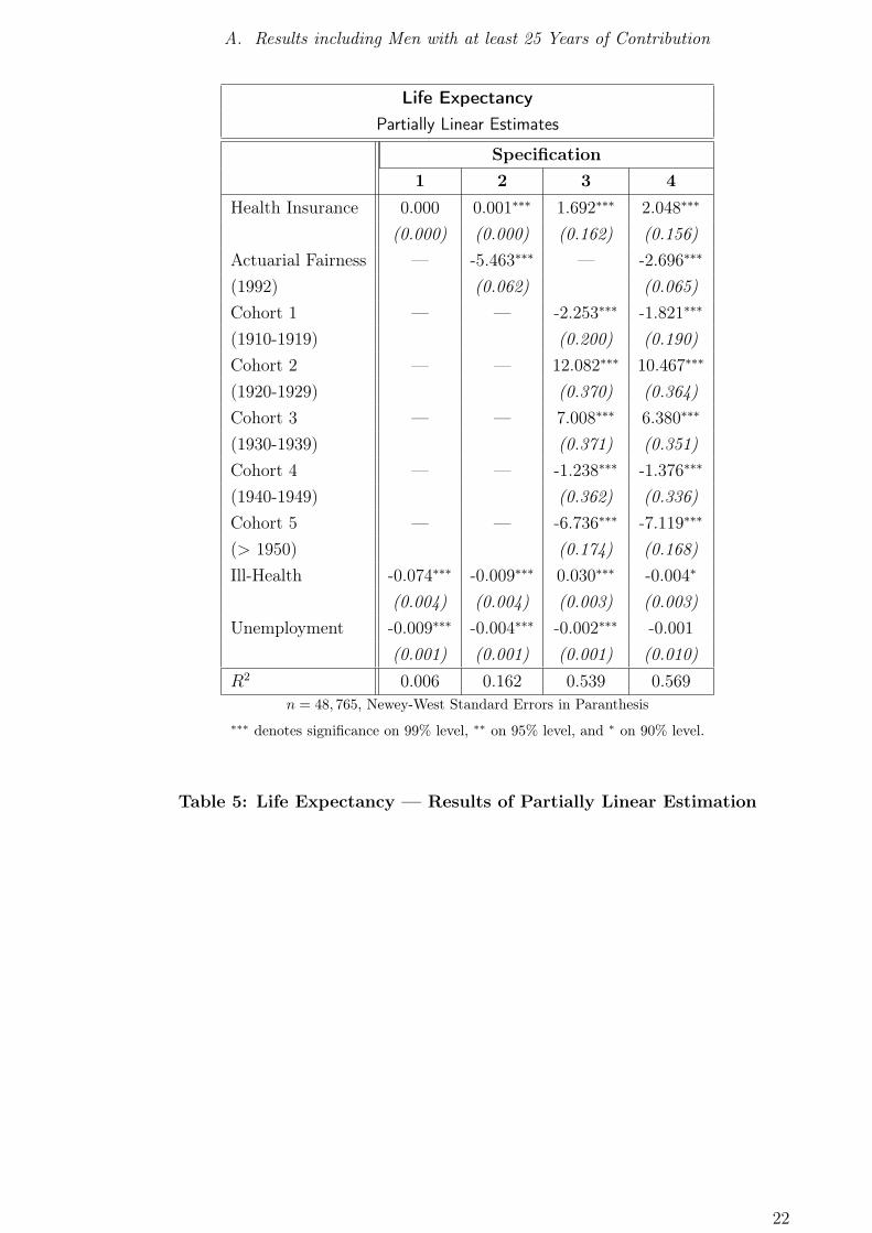
Results: Partially Linear Regression of Age on Benefit Claims Compare table 8
and figures 5 and 8 for the results of the partially linear model with age as dependent
variable.
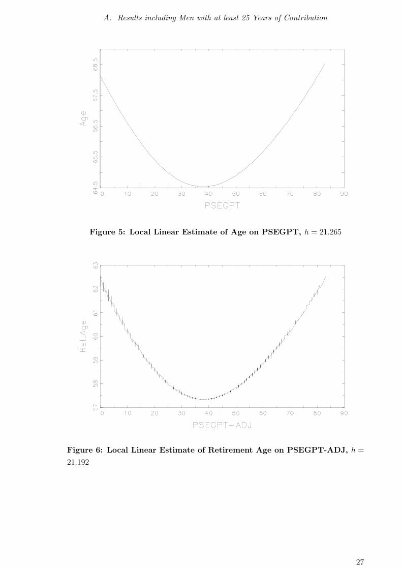
In the local linear estimation without additional regressors, a monotonously positive
relationship can only be discovered for individuals with claims beyond approximately
38 points. However, note that beyond 70 points there very few observations, such that
the majority of the observations can be found in the U -shaped part of the estimated
function. This pattern can be found again in all partially linear estimation results,
however, less pronounced. A private health insurance might be taken as an additional
indicator for high income, as only high income individuals are allowed to be privately
insured. However, conditional on higher income, a private health insurance is also an
indicator for good health, as private health insurers can discriminate their customers
regarding their health status, such that it might not be worthwhile for those in bad
health to buy private insurance. Accordingly, the existence of a private health insur-
ance is associated with higher life expectancy. Also unemployment, which is either an
indicator for low productivity, or even exerts direct pressure on an individual’s status
(regarding health, income and social status in general), lowers life expectancy in all
estimated specifications. Time spent in ill-health also lowers life expectancy, except
in specification 3. Including cohort effects does not change the main results; yet, the
coefficients of the respective cohort dummies cannot be directly interpreted in terms
of rising life expectancy through the years (which does not show up in the results as
well). The interpretation has be conditioned on the fact that there are no birth co-
horts considered, but rather a cohort of individuals who have died; so a cohort effect is
always conditional on reaching at least the year 1993, no matter when the individual
was born, which explains the negative coefficient of the youngest cohort (those born in
1950 and later).
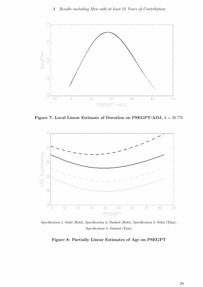
The U -shaped relation between collected claims and life expectancy especially around
the mean is astonishing and calls for explanation. Low life time earnings in terms of
collected claims against the public pension system can either be explained by low yearly
earnings, or by a short contribution period. An artifact of the German public pension
system is that certain professions which are traditionally performed self-employed are
eligible to opt out of the public pension system. Among those professions are some
which are typically well-paid, such as advocates, medical doctors or careers in the public
service. Individuals in these professions contribute more by chance than deliberately
to the public pension system in some (usually early) stages in their career, such that
they appear to have had a low income, but actually belong to the better (and best)
educated and earning individuals, though still included in the lowest PSEGPT region.
However, this conjecture cannot be corroborated, as we consider only individuals with
at least 25 years of work in a job where contributions to the public pension system
are mandatory. So a second conjecture utilizes the relatively rigid hourly wages in
14

5. Implementation and Results
Germany, especially at the lower end of the income distribution. An individual with
low life time earnings may have worked fewer hours per week than an individual with
intermediary life time earnings, while facing a comparable hourly wage. So the increase
in life time earnings from 10 to 20 points, e. g., is not due to an increase in productivity,
but due to an increase in hours worked, which by itself does not add to life expectancy.
To sum up, hypothesis 1 (Age) can only be corroborated for observations with more
than 38 collected points of benefit claims and must be rejected in general.
Results: Partially Linear Regression of Retirement Age on Benefit Claims This
estimation comes potentially twofold, as the data set offers different possibilities to
interpret the retirement age. Firstly, retirement age is the age at which an individual
receives his first benefit payment, which can be either the old-age pension or a disabil-
ity pension. Secondly, the age at entry into the "actual" pension is observed, which
constitutes the benefit payments that are paid until the end of the pensioner’s life,
and which can again be either one of both named types. In some cases, both pensions
might coincide, but not necessarily in general, such that an individual might receive
two or even more pension types during his life as a beneficiary. In order to capture the
meaning of hypothesis 2, the first concept is preferred (this applies to the estimation
regarding duration as well). Consider a worker who becomes unable to work at the
age of 55 and receives the respective pension benefit. At the age of 65, the benefits
are changed into the old-age pension; so if the second concept of retirement age were
applied, the reaction to an incentive (or necessity) for people with ill-health to retire
early could only be observed partially.
The results of these estimations can be found in the figures 6 and 9, as well as in
table 9. The final construction of the nonparametric (local linear) relationship between
retirement age and benefit claims yields again a strongly pronounced U -shaped pattern:
A monotonously increasing relationship can only be observed for those individuals who
collected more than 38 points of benefit claims, such that in specification 0, hypothesis
2 must generally be rejected.
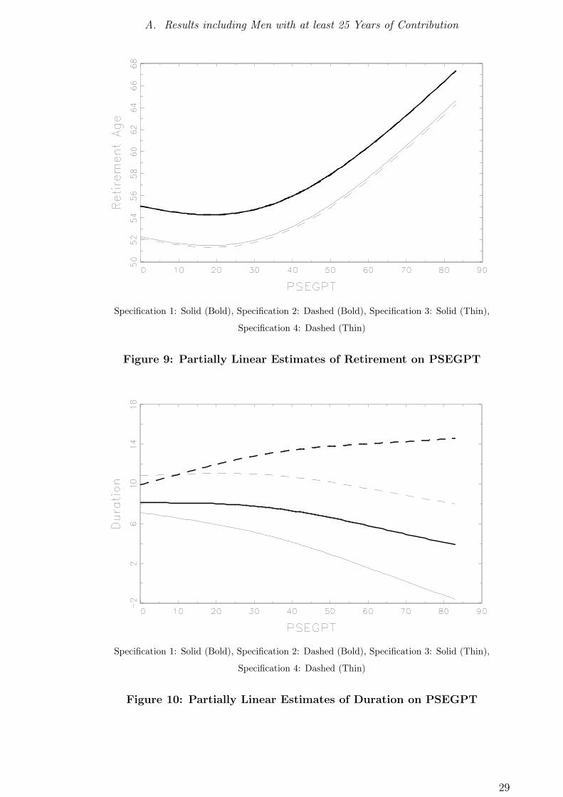
Including additional regressors, the shape of the relationship changes. Although a
monotonously increasing relationship can still not be found, the estimated minimum
retirement age is at approximately 20 points and increasing thereafter. Individuals
with private health insurance retire earlier, which is not in line with expectations. The
introduction of discounts for those who retire early, however, resulted in adaption of
the individuals, which retired later after the legislation in 1992. Yet, the reaction is
smaller as measured by Berkel and Börsch-Supan (2004), e. g., while the difference
crucially depends on the different data set and sub-sample. Time spent in ill-health
lowers the retirement age, which justifies hypothesis 2, whereas unemployment actually
increases the retirement age. This might be due to institutional factors, depending on
the possibilities of substitution between early retirement and unemployment at the
end of a career. Also possible is a dominating income effect at the lower end of the
15
5. Implementation and Results
income distribution, such that certain individuals cannot afford to retire earlier as they
do not want to face any discount. Finally, even in the partially linear specifications,
hypothesis 2 must be rejected in general, although the upward sloping relationship
dominates and encompasses the majority of individuals (compare again the histogram
of claims, figure 4).
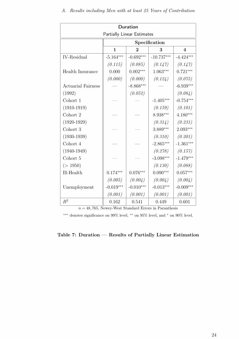
Results: Partially Linear Regression of Duration under the Benefit Spell on
Benefit Claims The results of the estimations can be found in figures 7 and 10,
as well as in table 10. The local linear estimate exerts a strong, inverted U -shaped
pattern, which does not appear in any of the partially linear specifications.
First of all, the IV-residuals appear to have a coefficient significantly different from
zero, such that the assumption of endogeneity of PSEGPT is justified also with dura-
tion as left-hand variable. Specifications 1, 3, and 4 yield a downward sloping curve,
meaning that there is no redistribution from poor to rich, as the duration and therefore
the rate of return decreases slightly with income. Yet, specification 2 indicates exactly
the opposite, namely a slightly increasing relationship between duration and collected
claims. A private health insurance is associated with a longer duration. Time spent
in ill-health is positively related to duration, off-setting the corresponding lower life
expectancy. Hence, paying pensions to early retirees who are potentially in bad-health
enhances their rate of return. Unemployment lowers the duration, which may be due
to institutional factors. A dramatic decrease in the duration is caused by the introduc-
tion of discounts for early retirees - however, this decrease is (in absolute terms) larger
for retirees with more than the average amount of collected claims, such that ceteris
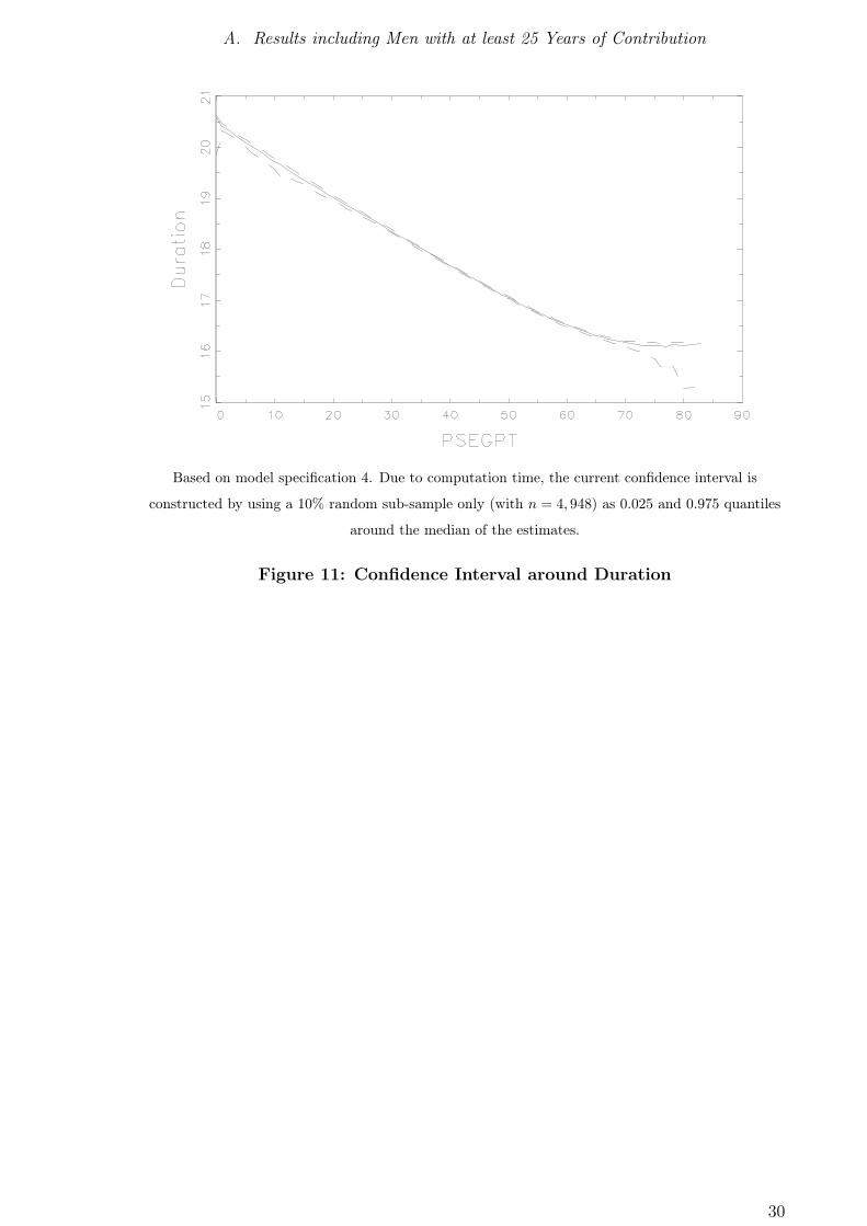
paribus the status of poorer individuals was relatively improved.16 For specification 4,
a confidence interval is constructed by the method proposed in section 4; see figure 11.
To sum up, there is neither clear evidence for an upward sloping relationship between
claims and duration, nor for a downward sloping one. However, all specifications
indicate that the duration is not orthogonal with respect to collected claims.
Robustness Note that all patterns are not an artifact of the estimation technique;
the general shape is corroborated by fitting a global polynomial of degree three by
least squares, and by replacing the local linear estimates of the conditional moments
by lowess or Nadaraya-Watson estimates. Plots of the distribution of the dependent
variables by PSEGPT-quantiles are not monotonously ordered, which also indicates a
more complex relation. Even the inclusion of women with at least 25 years of contribu-
tions does not alter the major results; however, the number of women in the analyzed
cohorts with such a career pattern is comparably low (∼ 10,000).
16Less than average PSEGPT is observed for 24,928 observations, 23,837 observations have higherclaims. The respective coefficients for the introduction of actuarial fairness in 1992 are in specifi-cation 2: -7.702 for the "poor" and -9.306 for the "rich", in specification 4: -5.026 for the "poor"and -7.697 for the "rich". The differences are significant.
16
6. Summary
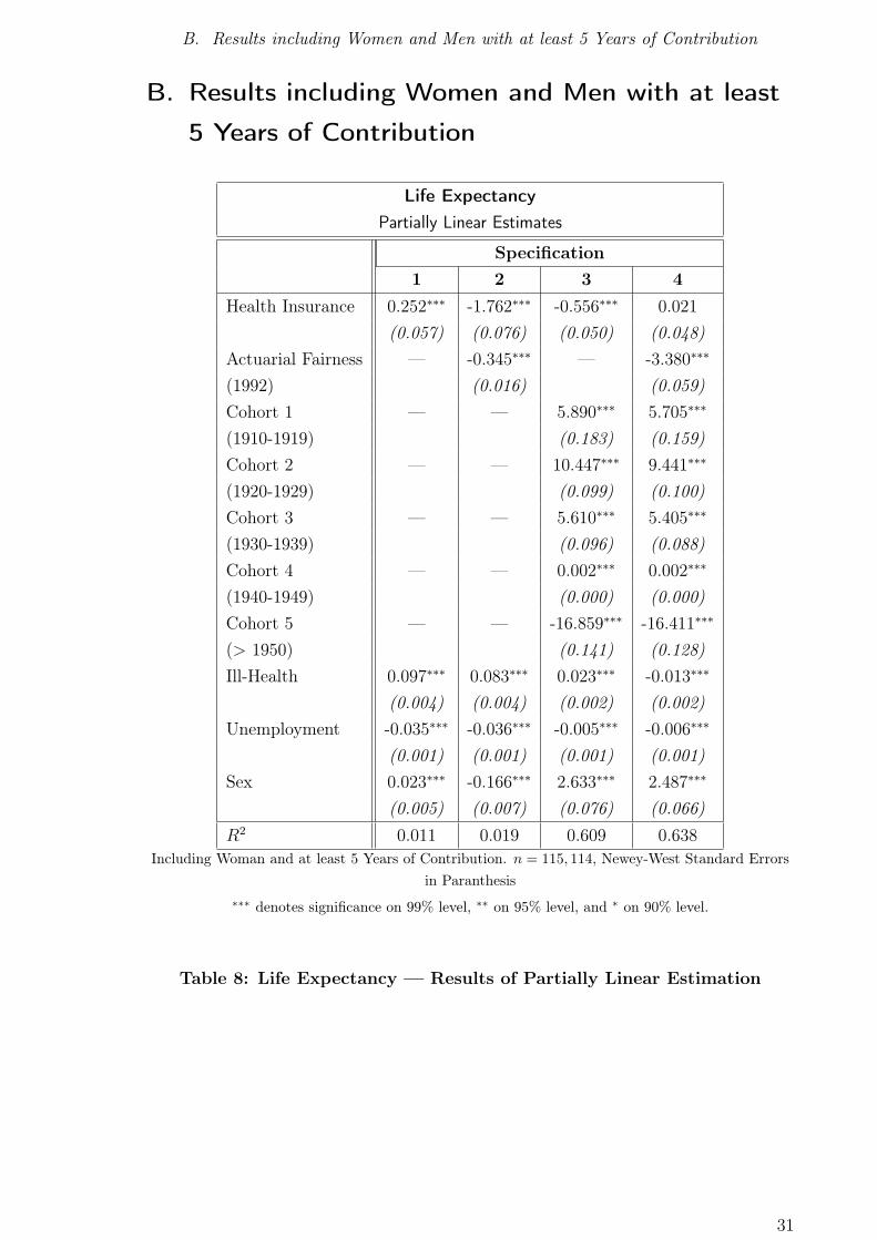
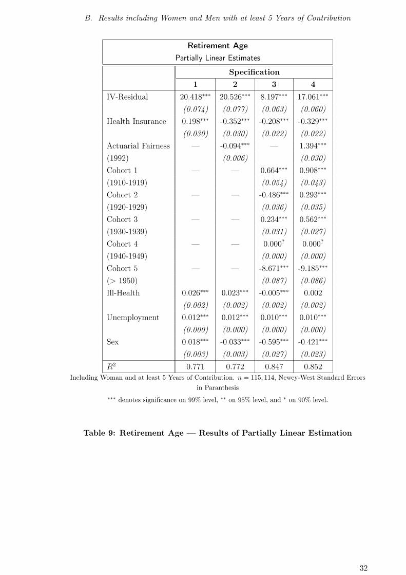
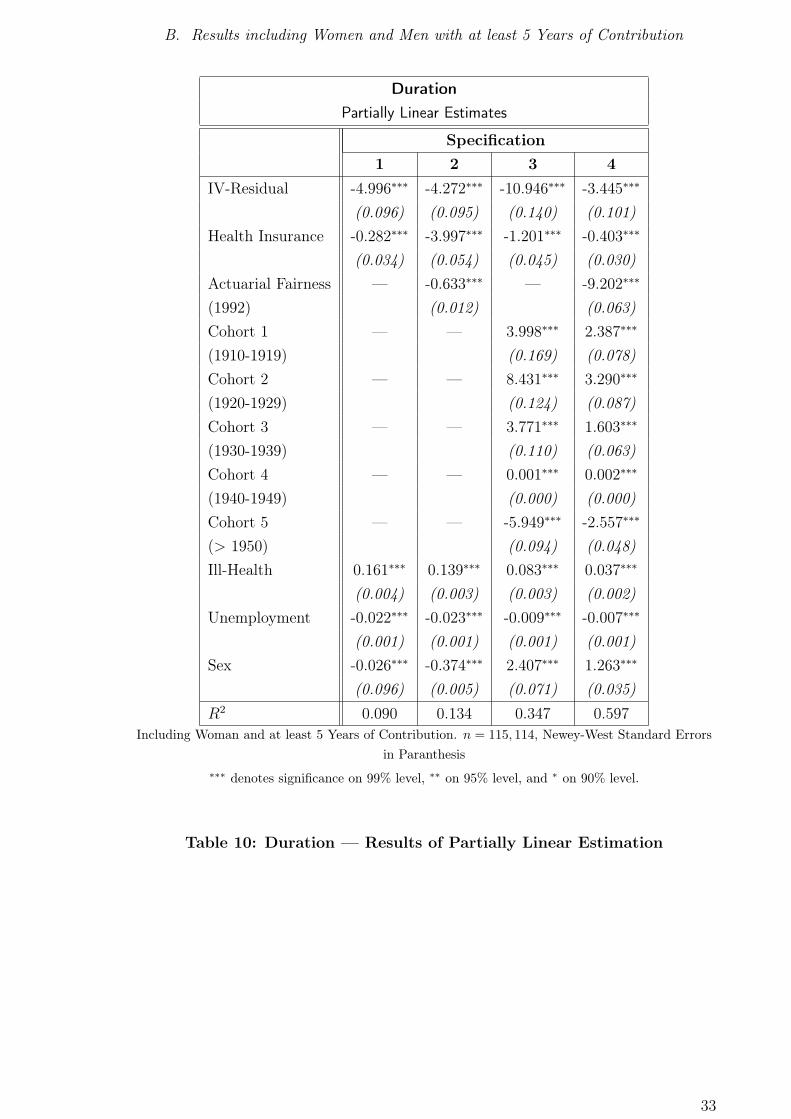
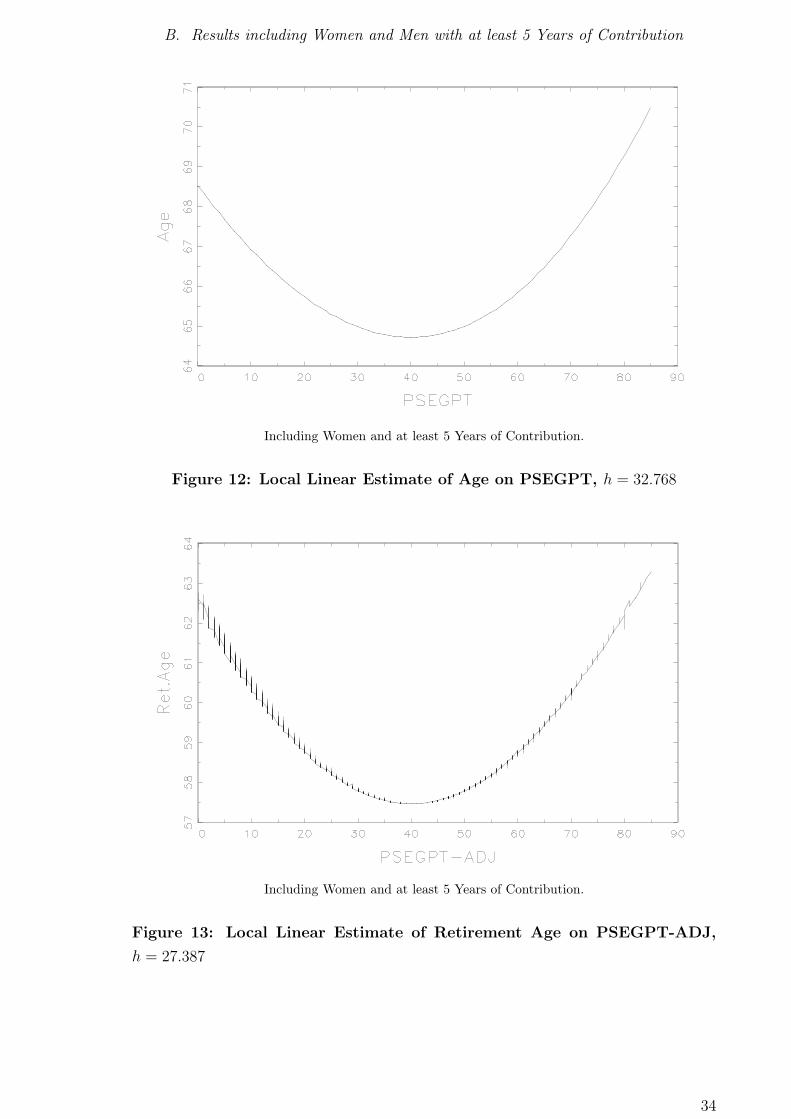
The results are also relatively robust against the selection of the sub-sample used
in the estimation. If the desired minimum of contribution is reduced to 5 years and
including women, the results shown in appendix B are obtained. The respective esti-
mates are based on 115,114 observations. The four specifications of the partially linear
model remain the same, except of the introduction of sex as an additional dummy
variable. The relationship of life expectancy and retirement age with benefit claims
does not change in its general shape, however, the local linear estimate of duration
(given benefit claims) is now monotonously increasing. The patterns derived from the
partially linear estimation are again very similar to the ones shown in appendix A, only
that now all four specifications yield a decreasing relationship of duration and benefit
claims. Out of 84 coefficients which are estimated, 23 change (significantly) their sign
due to the change of the sub-sample.
6. Summary
Life expectancy is not monotonously increasing in income (as measured by claims
against the public pension system), neither is retirement age. The relationships we
find are nevertheless robust. Especially around the mean of the collected claims, the
relation between life expectancy and collected claims is U -shaped, which calls for an
explanation. It can be shown that this pattern can be observed for the estimated
influence of collected claims on retirement age as well, and that this pattern is nei-
ther artefact of the data set, nor of the estimation procedure. Similar (however, also
rougher) findings can be derived by fitting a global polynomial and by survival analysis.
A conjectured explanation can be found in the rigidity of hourly wages in lowest
income groups: Most jobs which give rise to mandatory contributions to the pension
system are subject to collective wage bargaining. It can be argued that especially the
lowest wages are higher than wages which would arise on a perfect labor market. If
an individual belongs to the very bottom of the distribution of benefit claims (but still
has worked for more than 20 years), this is due to relatively low hourly wages and few
weekly hours of work. In order to move to the right on the claims distribution, the
increase in hourly wages is potentially small or close to zero; yet, individuals simply
work more hours, which does not add to life expectancy. Only beyond a certain level
(when full-time jobs are reached), higher income is associated with higher hourly wages
and not with more work time, which then increases life expectancy. Unfortunately, this
conjecture cannot be analyzed directly, as hours of work are not surveyed in this setting.
The estimated relationship between retirement age and benefit claims also shows
a U -shaped pattern. Although the non-actuarial discounts seem to encourage early
retirement at the margin, this might not be true for those at the bottom of the income
distribution: Every discount, even if it is relatively low, is not affordable due to a
required (or desired) minimum level of the pension benefits. Therefore, individuals
17
6. Summary
at the bottom of the income distribution choose to retire late, although they might
suffer from high disutility of labor. Only individuals in the intermediary sections of the
income distribution can actually afford to retire early, whereas those at the top have a
low disutility of labor (and are in good health), and accordingly retire late.
Finally, in three of four specifications the duration under the benefit spell is nega-
tively associated with claims, and only in one specification a positive relationship can
be found. A general mechanism which links income to a higher rate of return (or
less implicit taxation) from the public pension system can therefore not be corrobo-
rated. However, since the distributions of the duration and the collected claims are not
independent, the pension system is not redistributionally neutral.
Yet, there are two major factors which have not been considered yet. Firstly, the
whole analysis is conditional on reaching retirement age. Clearly, many individuals die
without ever having received benefits, and their fraction might depend on the size of
collected benefits. However note that all individuals are included who receive disability
benefits, which weakens the counter argument. Secondly, pensions paid to widows and
orphans are excluded, although their potential payment constitutes an asset to the
(altruistic) contributor. Unfortunately, within the used data set, their value cannot be
assessed individually.
18

A. Results including Men with at least 25 Years of Contribution
A. Results including Men with at least 25 Years of
Contribution
Variables in Data Set
Name Description Characteristics
(if not self-explanatory)
SK Label of Dataset always 90
JA Year of Report
CASE Case Number
FMSD Marital Status
GBJAVS Year of Birth (Insurant)
GBMOVS Month of Birth (Insurant)
GEVS Sex (Insurant)
SAVS Nationality (Insurant)
BFKL Profession 2 Digits
BLAND Residence (Federal State)
REGBEZ Residence (District)
GBJABC Year of Birth (Beneficiary)
GBMOBC Month of Birth (Beneficiary)
GEBC Sex (Beneficiary)
SABC Nationality (Beneficiary)
RTBE1 Year of 1st Pension Payment
ZTPR1 Year of Actual Pension Payment
RTWF1 Year of Discontinuation
RTWF2 Month of Discontinuation
AT Type of Health Insurance i. e., private or public insurance
EKAH Own Income if widowed joint payment of own pension
and widower’s pension
ZLKL1 Number of Children if parenting is assessed, up to 5
FRGLD Foreign Contributions especially former GDR
PSEGPT Sum of Collected Claims in points
WIRTZQ Bonus for Children if widowed in points
BYVL Full Years of Contribution up to 45
AUAZ Ill-Health up to 48 (months)
AJAZ Unemployment up to 120 (months)
FRGMO Foreign Contribution up to 45 (years)
POP Population Code own or widower’s pension
SATZ Type of Dataset always 2
Table 1: Variables FDZ-RV-SUFRTWF93VWITD to FDZ-RV-
SUFRTWF03VWITD
19
A. Results including Men with at least 25 Years of Contribution
Descriptive Statistics
Variable Raw Data Adjusted Data (if feasible)
Mean/Fractions St. Dev. Mean/Fractions St. Dev.
FMSD not married: 8.11%
married: 18.93%
GBJAVS 1917.87 11.57
GEVS female: 37.23%
SAVS Germany: 95.67%
EU-15 1.74%
Italy: 0.85%
Turkey: 0.24%
BLAND West: 76.78% West: 91.86%
East: 18.99% East: 1.77%
foreign: 3.59% foreign: 3.05%
GBJABC 1918.93 10.76 1934.70 5.80
GEBC female: 61.97% female: 0.00%
SABC Germany: 95.76% Germany: 90.93%
EU-15 1.76% EU-15 2.60%
Italy: 0.83% Italy: 1.32%
Turkey: 0.22% Turkey: 0.76%
RTBE1 1978.47 11.45 1993.00 5.54
ZTPTR1 1987.78 9.20 1995.70 2.78
AT private: 4.50% private: 10.80%
public: 86.23% public: 78.59%
FRGLD none: 94.73% none: 100.00%
former GDR: 0.44%
PSEGPT 32.53 19.12 43.22 13.05
BYVL 5.24 11.99 38.11 5.98
AUAZ 0.57 2.97 2.99 6.39
AJAZ 1.25 8.16 9.24 20.32
FRGMO 0.33 3.08 0.06 1.16
POP insurant: 30.80 % insurant: 100%
Generated Variables:
AGE 80.38 11.31 64.84 6.10
RET. AGE 59.54 8.15 57.75 5.25
DUR 20.32 11.18 7.10 5.63
Ret. ≥ 1992 74.41%
Cohort 1900-1909 0.10%
Cohort 1910-1919 0.27%
Cohort 1920-1929 18.03%
Cohort 1930-1939 63.99%
Cohort 1940-1949 15.53%
Cohort >1950 2.08% 20
A. Results including Men with at least 25 Years of Contribution
Adjustment of Data Set
Variable Discarded Obs. Total Number of Obs.
POP if POP = 2 (Widow or Orphan) 262,465
GBJABC if Missing 463
GBMOBC if Missing 600
GEBC if Female 549,782
SABC if Missing 1,309
RTBE1 if Missing 42,582
ZTPTR1 if Missing 51,521
FRGLD if FRGLD = 13 (GDR) 3,662
FRGLD if FRGLD = else (foreign) 39,417
PSEGPT if PSEGPT ≥ 86 1,532
BYVL if BYVL < 25 (Contribution) 773,632
The number of observations is reduced to 48,765.
Table 3: Adjustment of Data Set
Expectations, conditional on PSEGPT
Estimates by Probit
Variable Constant Coefficient
Health Insurance -7.699 -7.946
Actuarial Fairness (’92) 0.396 0.006
Cohort 1910-1919 -0.748 -49.512
Cohort 1920-1929 0.075 -7.102
Cohort 1930-1939 -0.656 -12.627
Cohort 1940-1949 -1.180 -7.162
Cohort > 1950 -2.948 -9.998
IV Estimation Step 1
Dependent Variable: PSEGPT
Variable Coefficient St. Error
PSEGPT-ADJ 1.010 0.000
Table 4: First Stage Results
21
A. Results including Men with at least 25 Years of Contribution
Life Expectancy
Partially Linear Estimates
Specification
1 2 3 4
Health Insurance 0.000 0.001∗∗∗ 1.692∗∗∗ 2.048∗∗∗
(0.000) (0.000) (0.162) (0.156)
Actuarial Fairness — -5.463∗∗∗ — -2.696∗∗∗
(1992) (0.062) (0.065)
Cohort 1 — — -2.253∗∗∗ -1.821∗∗∗
(1910-1919) (0.200) (0.190)
Cohort 2 — — 12.082∗∗∗ 10.467∗∗∗
(1920-1929) (0.370) (0.364)
Cohort 3 — — 7.008∗∗∗ 6.380∗∗∗
(1930-1939) (0.371) (0.351)
Cohort 4 — — -1.238∗∗∗ -1.376∗∗∗
(1940-1949) (0.362) (0.336)
Cohort 5 — — -6.736∗∗∗ -7.119∗∗∗
(> 1950) (0.174) (0.168)
Ill-Health -0.074∗∗∗ -0.009∗∗∗ 0.030∗∗∗ -0.004∗
(0.004) (0.004) (0.003) (0.003)
Unemployment -0.009∗∗∗ -0.004∗∗∗ -0.002∗∗∗ -0.001
(0.001) (0.001) (0.001) (0.010)
R2 0.006 0.162 0.539 0.569
n = 48, 765, Newey-West Standard Errors in Paranthesis
∗∗∗ denotes significance on 99% level, ∗∗ on 95% level, and ∗ on 90% level.
Table 5: Life Expectancy — Results of Partially Linear Estimation
22

A. Results including Men with at least 25 Years of Contribution
Retirement Age
Partially Linear Estimates
Specification
1 2 3 4
IV-Residual 15.848∗∗∗ 15.840∗∗∗ 15.583∗∗∗ 15.384∗∗∗
(0.074) (0.070) (0.074) (0.073)
Health Insurance -0.001∗∗∗ -0.001∗∗∗ -0.336∗∗∗ -0.325∗∗∗
(0.000) (0.000) (0.025) (0.025)
Actuarial Fairness — 0.017 — 0.219∗∗∗
(1992) (0.031) (0.031)
Cohort 1 — — -1.201∗∗∗ -1.221∗∗∗
(1910-1919) (0.036) (0.038)
Cohort 2 — — 2.681∗∗∗ 2.831∗∗∗
(1920-1929) (0.072) (0.079)
Cohort 3 — — 2.980∗∗∗ 3.037∗∗∗
(1930-1939) (0.068) (0.072)
Cohort 4 — — 3.052∗∗∗ 3.004∗∗∗
(1940-1949) (0.071) (0.072)
Cohort 5 — — -1.641∗∗∗ -1.693∗∗∗
(> 1950) (0.068) (0.068)
Ill-Health -0.010∗∗∗ -0.010∗∗∗ -0.017∗∗∗ -0.016∗∗∗
(0.003) (0.003) (0.003) (0.003)
Unemployment 0.012 0.012∗∗∗ 0.011∗∗∗ 0.011∗∗∗
(0.074) (0.001) (0.001) (0.001)
R2 0.839 0.839 0.859 0.859
n = 48, 765, Newey-West Standard Errors in Paranthesis
∗∗∗ denotes significance on 99% level, ∗∗ on 95% level, and ∗ on 90% level.
Table 6: Retirement Age — Results of Partially Linear Estimation
23
A. Results including Men with at least 25 Years of Contribution
Duration
Partially Linear Estimates
Specification
1 2 3 4
IV-Residual -5.164∗∗∗ -0.692∗∗∗ -10.737∗∗∗ -4.424∗∗∗
(0.115) (0.085) (0.147) (0.147)
Health Insurance 0.000 0.002∗∗∗ 1.063∗∗∗ 0.721∗∗∗
(0.000) (0.000) (0.124) (0.075)
Actuarial Fairness — -8.868∗∗∗ — -6.939∗∗∗
(1992) (0.052) (0.084)
Cohort 1 — — -1.405∗∗∗ -0.754∗∗∗
(1910-1919) (0.159) (0.101)
Cohort 2 — — 8.938∗∗∗ 4.180∗∗∗
(1920-1929) (0.314) (0.231)
Cohort 3 — — 3.889∗∗∗ 2.093∗∗∗
(1930-1939) (0.310) (0.201)
Cohort 4 — — -2.865∗∗∗ -1.361∗∗∗
(1940-1949) (0.278) (0.157)
Cohort 5 — — -3.098∗∗∗ -1.479∗∗∗
(> 1950) (0.130) (0.088)
Ill-Health 0.174∗∗∗ 0.076∗∗∗ 0.090∗∗∗ 0.057∗∗∗
(0.005) (0.004) (0.004) (0.004)
Unemployment -0.019∗∗∗ -0.010∗∗∗ -0.013∗∗∗ -0.009∗∗∗
(0.001) (0.001) (0.001) (0.001)
R2 0.162 0.541 0.449 0.601
n = 48, 765, Newey-West Standard Errors in Paranthesis
∗∗∗ denotes significance on 99% level, ∗∗ on 95% level, and ∗ on 90% level.
Table 7: Duration — Results of Partially Linear Estimation
24
A. Results including Men with at least 25 Years of Contribution
Figure 1: Histogram of Age
Figure 2: Histogram of Retirement Age
25
A. Results including Men with at least 25 Years of Contribution
Figure 3: Histogram of Duration
Figure 4: Histogram of PSEGPT
26
A. Results including Men with at least 25 Years of Contribution
Figure 5: Local Linear Estimate of Age on PSEGPT, h = 21.265
Figure 6: Local Linear Estimate of Retirement Age on PSEGPT-ADJ, h =
21.192
27
A. Results including Men with at least 25 Years of Contribution
Figure 7: Local Linear Estimate of Duration on PSEGPT-ADJ, h = 20.776
Specification 1: Solid (Bold), Specification 2: Dashed (Bold), Specification 3: Solid (Thin),
Specification 4: Dashed (Thin)
Figure 8: Partially Linear Estimates of Age on PSEGPT
28
A. Results including Men with at least 25 Years of Contribution
Specification 1: Solid (Bold), Specification 2: Dashed (Bold), Specification 3: Solid (Thin),
Specification 4: Dashed (Thin)
Figure 9: Partially Linear Estimates of Retirement on PSEGPT
Specification 1: Solid (Bold), Specification 2: Dashed (Bold), Specification 3: Solid (Thin),
Specification 4: Dashed (Thin)
Figure 10: Partially Linear Estimates of Duration on PSEGPT
29
A. Results including Men with at least 25 Years of Contribution
Based on model specification 4. Due to computation time, the current confidence interval is
constructed by using a 10% random sub-sample only (with n = 4, 948) as 0.025 and 0.975 quantiles
around the median of the estimates.
Figure 11: Confidence Interval around Duration
30
B. Results including Women and Men with at least 5 Years of Contribution
B. Results including Women and Men with at least
5 Years of Contribution
Life Expectancy
Partially Linear Estimates
Specification
1 2 3 4
Health Insurance 0.252∗∗∗ -1.762∗∗∗ -0.556∗∗∗ 0.021
(0.057) (0.076) (0.050) (0.048)
Actuarial Fairness — -0.345∗∗∗ — -3.380∗∗∗
(1992) (0.016) (0.059)
Cohort 1 — — 5.890∗∗∗ 5.705∗∗∗
(1910-1919) (0.183) (0.159)
Cohort 2 — — 10.447∗∗∗ 9.441∗∗∗
(1920-1929) (0.099) (0.100)
Cohort 3 — — 5.610∗∗∗ 5.405∗∗∗
(1930-1939) (0.096) (0.088)
Cohort 4 — — 0.002∗∗∗ 0.002∗∗∗
(1940-1949) (0.000) (0.000)
Cohort 5 — — -16.859∗∗∗ -16.411∗∗∗
(> 1950) (0.141) (0.128)
Ill-Health 0.097∗∗∗ 0.083∗∗∗ 0.023∗∗∗ -0.013∗∗∗
(0.004) (0.004) (0.002) (0.002)
Unemployment -0.035∗∗∗ -0.036∗∗∗ -0.005∗∗∗ -0.006∗∗∗
(0.001) (0.001) (0.001) (0.001)
Sex 0.023∗∗∗ -0.166∗∗∗ 2.633∗∗∗ 2.487∗∗∗
(0.005) (0.007) (0.076) (0.066)
R2 0.011 0.019 0.609 0.638
Including Woman and at least 5 Years of Contribution. n = 115, 114, Newey-West Standard Errors
in Paranthesis
∗∗∗ denotes significance on 99% level, ∗∗ on 95% level, and ∗ on 90% level.
Table 8: Life Expectancy — Results of Partially Linear Estimation
31
B. Results including Women and Men with at least 5 Years of Contribution
Retirement Age
Partially Linear Estimates
Specification
1 2 3 4
IV-Residual 20.418∗∗∗ 20.526∗∗∗ 8.197∗∗∗ 17.061∗∗∗
(0.074) (0.077) (0.063) (0.060)
Health Insurance 0.198∗∗∗ -0.352∗∗∗ -0.208∗∗∗ -0.329∗∗∗
(0.030) (0.030) (0.022) (0.022)
Actuarial Fairness — -0.094∗∗∗ — 1.394∗∗∗
(1992) (0.006) (0.030)
Cohort 1 — — 0.664∗∗∗ 0.908∗∗∗
(1910-1919) (0.054) (0.043)
Cohort 2 — — -0.486∗∗∗ 0.293∗∗∗
(1920-1929) (0.036) (0.035)
Cohort 3 — — 0.234∗∗∗ 0.562∗∗∗
(1930-1939) (0.031) (0.027)
Cohort 4 — — 0.000? 0.000?
(1940-1949) (0.000) (0.000)
Cohort 5 — — -8.671∗∗∗ -9.185∗∗∗
(> 1950) (0.087) (0.086)
Ill-Health 0.026∗∗∗ 0.023∗∗∗ -0.005∗∗∗ 0.002
(0.002) (0.002) (0.002) (0.002)
Unemployment 0.012∗∗∗ 0.012∗∗∗ 0.010∗∗∗ 0.010∗∗∗
(0.000) (0.000) (0.000) (0.000)
Sex 0.018∗∗∗ -0.033∗∗∗ -0.595∗∗∗ -0.421∗∗∗
(0.003) (0.003) (0.027) (0.023)
R2 0.771 0.772 0.847 0.852
Including Woman and at least 5 Years of Contribution. n = 115, 114, Newey-West Standard Errors
in Paranthesis
∗∗∗ denotes significance on 99% level, ∗∗ on 95% level, and ∗ on 90% level.
Table 9: Retirement Age — Results of Partially Linear Estimation
32
B. Results including Women and Men with at least 5 Years of Contribution
Duration
Partially Linear Estimates
Specification
1 2 3 4
IV-Residual -4.996∗∗∗ -4.272∗∗∗ -10.946∗∗∗ -3.445∗∗∗
(0.096) (0.095) (0.140) (0.101)
Health Insurance -0.282∗∗∗ -3.997∗∗∗ -1.201∗∗∗ -0.403∗∗∗
(0.034) (0.054) (0.045) (0.030)
Actuarial Fairness — -0.633∗∗∗ — -9.202∗∗∗
(1992) (0.012) (0.063)
Cohort 1 — — 3.998∗∗∗ 2.387∗∗∗
(1910-1919) (0.169) (0.078)
Cohort 2 — — 8.431∗∗∗ 3.290∗∗∗
(1920-1929) (0.124) (0.087)
Cohort 3 — — 3.771∗∗∗ 1.603∗∗∗
(1930-1939) (0.110) (0.063)
Cohort 4 — — 0.001∗∗∗ 0.002∗∗∗
(1940-1949) (0.000) (0.000)
Cohort 5 — — -5.949∗∗∗ -2.557∗∗∗
(> 1950) (0.094) (0.048)
Ill-Health 0.161∗∗∗ 0.139∗∗∗ 0.083∗∗∗ 0.037∗∗∗
(0.004) (0.003) (0.003) (0.002)
Unemployment -0.022∗∗∗ -0.023∗∗∗ -0.009∗∗∗ -0.007∗∗∗
(0.001) (0.001) (0.001) (0.001)
Sex -0.026∗∗∗ -0.374∗∗∗ 2.407∗∗∗ 1.263∗∗∗
(0.096) (0.005) (0.071) (0.035)
R2 0.090 0.134 0.347 0.597
Including Woman and at least 5 Years of Contribution. n = 115, 114, Newey-West Standard Errors
in Paranthesis
∗∗∗ denotes significance on 99% level, ∗∗ on 95% level, and ∗ on 90% level.
Table 10: Duration — Results of Partially Linear Estimation
33
B. Results including Women and Men with at least 5 Years of Contribution
Including Women and at least 5 Years of Contribution.
Figure 12: Local Linear Estimate of Age on PSEGPT, h = 32.768
Including Women and at least 5 Years of Contribution.
Figure 13: Local Linear Estimate of Retirement Age on PSEGPT-ADJ,
h = 27.387
34
B. Results including Women and Men with at least 5 Years of Contribution
Including Women and at least 5 Years of Contribution.
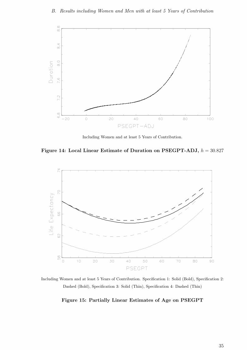
Figure 14: Local Linear Estimate of Duration on PSEGPT-ADJ, h = 30.827
Including Women and at least 5 Years of Contribution. Specification 1: Solid (Bold), Specification 2:
Dashed (Bold), Specification 3: Solid (Thin), Specification 4: Dashed (Thin)
Figure 15: Partially Linear Estimates of Age on PSEGPT
35
B. Results including Women and Men with at least 5 Years of Contribution
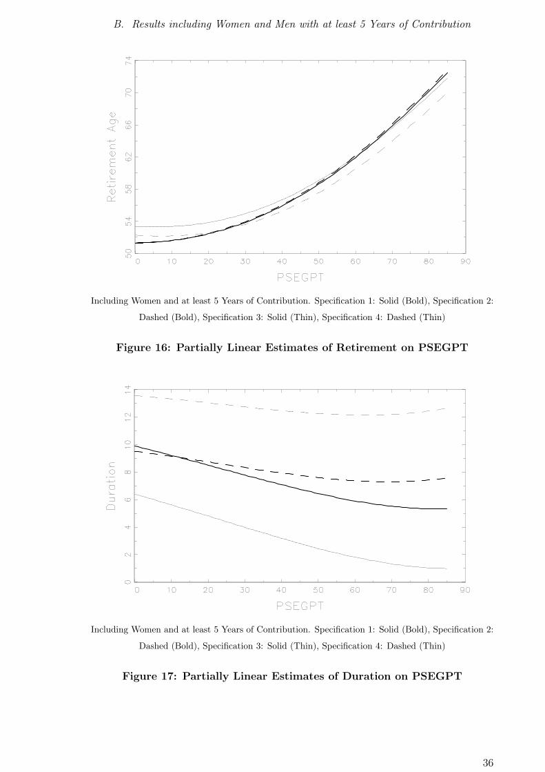
Including Women and at least 5 Years of Contribution. Specification 1: Solid (Bold), Specification 2:
Dashed (Bold), Specification 3: Solid (Thin), Specification 4: Dashed (Thin)
Figure 16: Partially Linear Estimates of Retirement on PSEGPT
Including Women and at least 5 Years of Contribution. Specification 1: Solid (Bold), Specification 2:
Dashed (Bold), Specification 3: Solid (Thin), Specification 4: Dashed (Thin)
Figure 17: Partially Linear Estimates of Duration on PSEGPT
36
References
References
Adams, P., M. D. Hurd, D. MacFadden, A. Merrill, and T. Ribeiro (2004):
“Healthy, wealthy and wise? Tests for direct causal paths between health and so-
cioeconomic status,” Journal of Econometrics, (112), 3–56.
Berkel, B., and A. Börsch-Supan (2004): “Pension Reform in Germany: The
Impact on Retirement Decisions,” FinanzArchiv, 60(3), 393–421.
Blundell, R., and A. Duncan (1998): “Kernel Regression in Empirical Microeco-
nomics,” The Journal of Human Resources, 33(1), 62–87.
Börsch-Supan, A., and R. Schnabel (1998): “Social Security and Declinign Labor-
Force Participation in Germany,” The American Economic Review, 88(2), 173–178.
Cremer, H., J.-M. Lozachmeur, and P. Pestieau (2004): “Social Security, Re-
tirement Age and Optimal Income Taxation,” Journal of Public Economics, 88,
2259–2281.
Cremer, H., and P. Pestieau (1996): “Redistributive Taxation and Social Insur-
ance,” International Tax and Public Finance, 3, 281–295.
Deaton, A., and C. Paxson (2004): “Mortality, Education, Income, and Inequality
among American Cohorts,” NBER Working Paper, (7140).
Diamond, P. A. (2003): Taxation, Incomplete Markets, and Social Security. MIT
Press, Cambrigde.
Grossman, M. (1972): “On the Concept of Health Capital and the Demand for
Health,” Jorunal of Political Economy, 80(2), 223–255.
Kommission zur Verbesserung der informationellen Infrastruktur
zwischen Wissenschaft und Statistik (2001): Wege zu einer besseren in-
formationellen Infrastruktur. Gutachten der vom Bundesministerium für Bildung
und Forschung eingesetzten Kommission zur Verbesserung der informationellen In-
frastruktur zwischen Wissenschaft und Statistik. Nomos, Baden-Baden.
Loader, C. (1999): Local Regression and Likelihood. Springer, New York.
Loader, C. (2004): “Smoothing: Local Regression Techniques,” in Handbook of Com-
putational Statistics, ed. by J. Gentle, W. Härdle, and Y. Mori. Springer.
Mittelhammer, R. C., G. G. Judge, and D. J. Miller (2000): Econometric
Foundations. Cambridge University Press, Cambridge.
Pagan, A., and A. Ullah (1999): Nonparametric Econometrics. Cambridge Univer-
sity Press, Cambridge.
37
References
Reil-Held, A. (2000): “Einkommen und Sterblichkeit in Deutschland: Leben Reiche
länger?,” Beiträge zur angewandten Wirtschaftsforschung, 580-00.
Ruppert, D., M. P. Wand, and R. J. Carroll (2003): Semiparametric Regression.
Cambridge University Press, Cambridge.
Schils, T. (2005): Early Retirement Patterns in Europe: A comparative Panel Study.
Dutch University Press, Amsterdam.
Yatchew, A. (1998): “Nonparametric Regression Techniques in Economics,” Journal
of Economic Literature, 36(2), 669–721.
(2003): Semiparametric Regression for the Applied Econometrician. Cam-
bridge University Press, Cambridge.
38