Disengagement: A partial solution to the annuity puzzle

Hazel Batemana

Christine Eckertb,c

John Gewekeb

Fedor Iskhakovb,d

Jordan Louviereb

Stephen Satchelle,f

Susan Thorp*b,g

March 27, 2013

a School of Risk and Actuarial Studies, University of New South Wales, 2052, Australia

b Centre for the Study of Choice, UTS Business School, 645 Harris Street, Ultimo, 2007, Aus-tralia

c Marketing Discipline Group, UTS Business School, Quay Street, Haymarket, 2000, Australia

d ARC Centre of Excellence in Population Aging Research, University of New South Wales,2052, Australia

e Trinity College, University of Cambridge, Cambridge, CB2 1TQ, U.K.

f Discipline of Finance, University of Sydney, 2006, Australia

g Finance Discipline Group, UTS Business School, Quay Street, Haymarket, 2000, Australia

* Corresponding author; Address: UTS Business School, University of Technology Sydney, POBox 123, Broadway, NSW 2007, Australia; Phone: +61 2 9514 7784; Fax: +61 2 9514 7711;Email: Susan.Thorp@uts.edu.au.

Email addresses: Bateman: h.bateman@unsw.edu.au; Eckert: christine.eckert@uts.edu.au; Geweke:john.geweke@uts.edu.au; Iskhakov: fedor.iskhakov@uts.edu.au; Louviere: jordan.louviere@uts.edu.au;Satchell: ses11@cam.ac.uk; Thorp: susan.thorp@uts.edu.au

1

Abstract

This research studies whether individuals make choices consistent with expected utilitymaximization in allocating wealth between a lifetime annuity and a phased withdrawal ac-count at retirement. The paper describes the construction and administration of a discretechoice experiment to 854 respondents approaching retirement. The experiment finds overallrates of inconsistency with the predictions of the standard CRRA utility model of roughly50%, and variation in consistency rates depending on the characteristics of the respondents.Individuals with poor numeracy and with low engagement with the choice task, as measuredby scores on a task-specific recall quiz, are more likely to increase allocations to the phasedwithdrawal as the risk of exhausting it increases. Individuals with higher scores on tests offinancial capability and with knowledge of retirement income products are more likely toscore high on the engagement measure, but capability and knowledge do not have indepen-dent effects on consistent choice rates. Results suggest that initiatives to improve specificproduct knowledge and to help individuals engage with decumulation decisions could be apartial solution to the annuity puzzle.

JEL classification: G23; G28; D14

Key words: discrete choice; retirement incomes; household finance; financial literacy;

2

1 Introduction

Most members of defined benefit (DB) pension plans enjoy a natural continuity in income

between work and retirement via pre-set annuity payments. By contrast, members of defined

contribution (DC) plans who want to insure against outliving their income must give up lump

sum savings in exchange for a lifetime annuity while still keeping some liquid assets to cover

uninsured events.

Despite strong theoretical support for lifetime annuity purchase (Yaari 1965; Davidoff et al.

2005; Horneff et al. 2007), the weak global demand for voluntary life annuities is a continu-

ing puzzle (Mitchell et al. 2011). The US and Australia, for example, both operate private

retirement savings schemes yet very few convert retirement accumulations to lifetime annuities:

only around 1% of US 401(k) plan retirees offered a life annuity actually purchase one (EBRI,

2011) and sales of life annuities in Australia stand at around 100 policies annually in a mar-

ket with several million retirees (Plan for Life 2012). The negligible demand for life annuities

is more surprising in Australia where virtually all workers save into mandatory individual DC

(superannuation) accounts and do not receive earnings-linked social security payments.

Academic research has not settled on a definitive explanation for the annuity puzzle. Theo-

retical studies cannot explain why even partial annuitization is rare1 and when empirical studies

show some demand for annuities it is often where the annuity is the default (Butler and Teppa

2007; Benartzi et al. 2012).2 More recently, research has turned to behavioral or psychological

explanations, surveyed in Brown (2008) and Benartzi et al. (2012). Behavioral explanations for

a lack of interest in annuities include mental accounting and loss aversion (Hu and Scott 2007),

susceptibility to information framing (Agnew et al. 2008; Brown et al. 2008; Cappelletti et

al. 2011; Beshears et al. 2012) and complexity (Brown et al. 2011). Here we expand on the

contributions of both conventional and behavioral research by testing how disengagement with

the retirement benefit decision affects annuity choice.

1Extensions to standard lifecycle models attribute low consumer interest in lifetime annuities to pricing issues(Mitchell et al. 1999), crowding out (Dushi and Webb 2004), bequests (Bernheim 1991), intra family risk sharing(Brown and Poterba 2001), demand for liquidity for uncertain health expenses (Turra and Mitchell 2008; Peijnen-burg et al. 2010) and the option value of delay (Kingston and Thorp 2005; Milevsky and Young 2007). However,Inkmann et al. (2011) do find theoretical support for low annuity demand for specific combinations of preferenceparameters.

2For example, using Swiss pension fund data Butler and Teppa (2007) a 90% annuity take up rate (73% fulland 17% partial) where the annuity is the default, compared with only 10% under a lump sum default.

3

Much previous research assumes that ordinary people know what retirement benefit products

are available and understand how they work. However, a preliminary survey we conducted

showed scant product awareness and minimal understanding of the main insurance features of

income streams: for example, only one third of respondents had heard of a life annuity, with only

20% and 8% aware of its longevity and income guarantee characteristics. Respondents showed

similar ignorance of other retirement income products such as phased withdrawals.3

A lack of understanding is not surprising. A life annuity is a complex, one-in-a-lifetime

product, unfamiliar to most pre-retirees. The recent switch to DC plans means that there has

been limited opportunity for social learning among the current generation (Bernheim 2002).

Unlike other major financial decisions, such as house purchases, older generations have little

experience with managing an accumulation lump sum and cannot give advice. Further, the

retirement benefit decision involves high stakes (often the household’s largest non-housing asset)

and is typically made only once, often irreversibly, which prevents people learning from past

experience (Beshears et al 2008). In addition, purchasing retirement products from a menu

is a difficult financial decision usually needing immediate action but having consequences well

into the future (Beshears et al. 2008). The relationship between both financial capability and

financial outcomes (Lusardi and Mitchell 2009, 2011; Gerardi et al. 2010; Guiso and Jappelli

2008), and specific product knowledge and retirement saving decisions (Gustman et al. 2012;

Cappelletti et al. 2011), is well established. Moreover, Brown et al. (2011) confirm that

people with low financial literacy are particularly confused by life annuities. It is likely that

most ordinary members of DC plans have not learned what they really need to know about life

annuities or other retirement benefit products by the time they are ready to retire.

Motivated by the complexity of life annuities, we investigate the impact of plan member

interest and specific product understanding on the quality of retirement benefit choices, and

particularly, the demand for annuities. We design and implement a discrete choice experiment

on benefit decisions through a survey panel of 854 near-to-retirement DC plan members from

Australia. Each survey respondent chooses the percentage of financial wealth to allocate to two

retirement income streams: a liquid phased withdrawal account invested in risky assets and a life

3The survey was conducted on a representative sample of 920 Australian pre-retiree superannuation (pension)fund members aged 50-74 and was designed to collect information about consumer awareness and understandingof retirement income products available in the Australian market.

4

annuity with or without a guarantee period. Respondents make two sets of pairwise allocations

(phased withdrawal v. life annuity, then phased withdrawal v. period certain annuity) at four

risk levels. The risk they confront is the chance of running out of money in the phased withdrawal

account before the end of life, and consequently having to live on a reduced income. Income

from the annuities is guaranteed but income from the phased withdrawal may be exhausted. The

result is two sequences of four wealth allocations revealing respondents’ changing preferences for

guaranteed income and liquidity as the risk of exhausting the liquid account increases.

We approach the annuity decision differently from previous studies. First, we do not pre-

sume that individuals approaching retirement know and understand retirement benefit products.

Instead, we show respondents a clear explanation and comparison of the alternative products

in terms of five common features. Second, rather than offering an ‘all or nothing’ annuitiza-

tion decision, we let people explore a continuum of partial annuitization options. Respondents

can trade-off the benefits of a non-annuitized product (phased withdrawal), such as access to

liquid balances and continued exposure to investment risk, against the benefits of a constant,

lifetime income stream (life annuity).4 Third, under this experimental design, where reductions

in income due to exhausting resources are significant and permanent, and respondents allocate

all financial wealth at retirement, risk aversion over income should be significant. Hence we

can evaluate whether the sequence of retirement wealth allocation decisions are consistent with

some implications of CRRA utility maximization. A simple indicator of consistency is whether

we see respondents choosing no less longevity insurance as the probability of exhausting liquid

balances before the end of life increases. This condition tests whether respondents grasp the

main insurance feature of the annuity.

Finally, in our estimation of decision consistency, we specifically measure and take account

of engagement with the experimental task. In any choice experiment, data quality depends on

respondents’ ‘real-time’ interest in the task at hand. It is likely that the choices of individuals

who are uninterested distort results. Many experiments use monetary rewards to create interest

and align incentives (Camerer and Hogarth, 1999) but few embed direct tests of task engagement.

Here we introduce an individual task engagement measure: we collect scores from a short recall

4In our experiment respondents choose from a vector of allocations to each product that increase from 0% to100% in increments of 5 percentage points. Beshears et al (2012) provide a similar setup with increments of 25percentage points.

5

quiz that tests knowledge of the five common features of the retirement products in the allocation

experiment.5 The recall quiz reviews survey-specific information about the annuities and phased

withdrawal that respondents should read just before the task. Quiz scores measure whether the

respondent is engaging with the choice task, and at the same time show how capable they

are of comparing the products effectively. If a respondent cannot recall the vital features of the

products, they are likely to be disengaged and uninformed, and less likely to meet the consistency

condition.

This experiment allows us to assess the effect of disengagement on annuitization decisions.

In particular, we show how a lack of engagement and the resultant lack of specific product

knowledge limits people’s ability to manage retirement income risk and consequently distorts

annuity choice. We also investigate how pre-existing numeracy and financial literacy help, and

to what extent. Overall the results show that pre-existing financial capability increases task

engagement, as measured by the recall quiz score, but consistent choices are directly explained

only by task engagement and numeracy. Engagement can help plan members learn the insurance

features of income stream products, so increasing their ability to perceive and manage retirement

risk.

Section 2 sets out a simple model of retirement wealth allocation used to design our discrete

choice experiment. Simulations using this model imply that certain allocation sequences should

not be observed for CRRA utility maximizers. In Section 3 we discuss the design and imple-

mentation of the on-line experiment, including the experimental task, the recall quiz designed to

test task engagement and questions that collect data on financial capability, commercial prod-

uct knowledge, health, longevity expectations, planning and demographics. Section 4 presents

our econometric model and findings. The final section reviews findings. It outlines tentative

conclusions about importance of task engagement in experimental settings, the links between

engagement and pre-existing financial capability, and the importance of both product-specific

knowledge and quantitative skills in decumulation decisions.

5This approach is informed by the idea of an Instructional Manipulation Check (IMC) as developed in Op-penheimer et al. (2009).

6

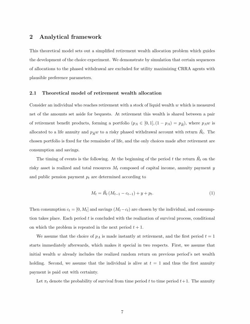
2 Analytical framework

This theoretical model sets out a simplified retirement wealth allocation problem which guides

the development of the choice experiment. We demonstrate by simulation that certain sequences

of allocations to the phased withdrawal are excluded for utility maximizing CRRA agents with

plausible preference parameters.

2.1 Theoretical model of retirement wealth allocation

Consider an individual who reaches retirement with a stock of liquid wealth w which is measured

net of the amounts set aside for bequests. At retirement this wealth is shared between a pair

of retirement benefit products, forming a portfolio (pA ∈ [0, 1], (1 − pA) = pR), where pAw is

allocated to a life annuity and pRw to a risky phased withdrawal account with return Rt. The

chosen portfolio is fixed for the remainder of life, and the only choices made after retirement are

consumption and savings.

The timing of events is the following. At the beginning of the period t the return Rt on the

risky asset is realized and total resources Mt composed of capital income, annuity payment y

and public pension payment pt are determined according to

Mt = Rt (Mt−1 − ct−1) + y + pt. (1)

Then consumption ct = [0,Mt] and savings (Mt−ct) are chosen by the individual, and consump-

tion takes place. Each period t is concluded with the realization of survival process, conditional

on which the problem is repeated in the next period t+ 1.

We assume that the choice of pA is made instantly at retirement, and the first period t = 1

starts immediately afterwards, which makes it special in two respects. First, we assume that

initial wealth w already includes the realized random return on previous period’s net wealth

holding. Second, we assume that the individual is alive at t = 1 and thus the first annuity

payment is paid out with certainty.

Let πt denote the probability of survival from time period t to time period t+1. The annuity

7

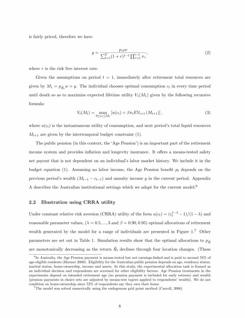
is fairly priced, therefore we have

y =pAw∑T

t=1(1 + r)1−t∏t−1τ=1 πτ

, (2)

where r is the risk free interest rate.

Given the assumptions on period t = 1, immediately after retirement total resources are

given by M1 = pRtw + y. The individual chooses optimal consumption ct in every time period

until death so as to maximize expected lifetime utility V1(M1) given by the following recursive

formula:

Vt(Mt) = max0≤ct≤Mt

[u(ct) + βπtEVt+1 (Mt+1)] , (3)

where u(ct) is the instantaneous utility of consumption, and next period’s total liquid resources

Mt+1 are given by the intertemporal budget constraint (1).

The public pension (in this context, the ‘Age Pension’) is an important part of the retirement

income system and provides inflation and longevity insurance. It offers a means-tested safety

net payout that is not dependent on an individual’s labor market history. We include it in the

budget equation (1). Assuming no labor income, the Age Pension benefit pt depends on the

previous period’s wealth (Mt−1 − ct−1) and annuity income y in the current period. Appendix

A describes the Australian institutional settings which we adapt for the current model.6

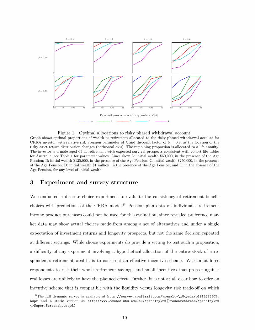
2.2 Illustration using CRRA utility

Under constant relative risk aversion (CRRA) utility of the form u(ct) = (c1−λt − 1)/(1−λ) and

reasonable parameter values, (λ = 0.5, ..., 3 and β = 0.90, 0.95) optimal allocations of retirement

wealth generated by the model for a range of individuals are presented in Figure 1.7 Other

parameters are set out in Table 1. Simulation results show that the optimal allocations to pR

are monotonically decreasing as the return Rt declines through four location changes. (These

6In Australia, the Age Pension payment is means-tested but not earnings-linked and is paid to around 76% ofage-eligible residents (Harmer 2009). Eligibility for the Australian public pension depends on age, residency status,marital status, home-ownership, income and assets. In this study, the experimental allocation task is framed asan individual decision and respondents are screened for other eligibility factors. Age Pension treatments in theexperiments depend on intended retirement age (no pension payment is included for early retirees) and wealth(pension payments in choice sets are adjusted by means-test tapers applied to respondents’ wealth). We do notcondition on home-ownership since 72% of respondents say they own their home.

7The model was solved numerically using the endogenous grid point method (Carroll, 2006)

8

are chosen to create a range of probabilities of exhausting the phased withdrawal before the end

of life for the experiment. They are set out in Table 1.) In cases of very low risk aversion, the

optimal allocation is at the 100% boundary. The result of lower allocations to pR as the return

declines holds over a wide range of wealth levels ($50,000-$1 million), when the retiree is eligible

for the public Age Pension (Figure 1, A-D) and when they are not (E). When the individual does

not receive the the public Age Pension, allocations to pR decline at faster rates. Means-testing

tapers encourage eligible retirees to substitute private annuity income for the public annuity

(public Age Pension) at higher levels of wealth. This simple model serves to benchmark income

and risk levels in the choice sets presented to respondents in the on-line experimental task.

9

0

1

A B C D E

0.001 0.03 0.063 0.1 0

1

0.001 0.03 0.063 0.1 0.001 0.03 0.063 0.1 0.001 0.03 0.063 0.1

Expected gross returns of r isky product, E [R]

β = 0.90

λ = 0.5 λ = 1.0 λ = 1.5 λ = 3.0

β = 0.90

Figure 1: Optimal allocations to risky phased withdrawal account.Graph shows optimal proportions of wealth at retirement allocated to the risky phased withdrawal account forCRRA investor with relative risk aversion parameter of λ and discount factor of β = 0.9, as the location of therisky asset return distribution changes (horizontal axis). The remaining proportion is allocated to a life annuity.The investor is a male aged 65 at retirement with expected survival prospects consistent with cohort life tablesfor Australia; see Table 1 for parameter values. Lines show A: initial wealth $50,000, in the presence of the AgePension; B: initial wealth $125,000, in the presence of the Age Pension; C: initial wealth $250,000, in the presenceof the Age Pension; D: initial wealth $1 million, in the presence of the Age Pension; and E: in the absence of theAge Pension, for any level of initial wealth.

3 Experiment and survey structure

We conducted a discrete choice experiment to evaluate the consistency of retirement benefit

choices with predictions of the CRRA model.8 Pension plan data on individuals’ retirement

income product purchases could not be used for this evaluation, since revealed preference mar-

ket data may show actual choices made from among a set of alternatives and under a single

expectation of investment returns and longevity prospects, but not the same decision repeated

at different settings. While choice experiments do provide a setting to test such a proposition,

a difficulty of any experiment involving a hypothetical allocation of the entire stock of a re-

spondent’s retirement wealth, is to construct an effective incentive scheme. We cannot force

respondents to risk their whole retirement savings, and small incentives that protect against

real losses are unlikely to have the planned effect. Further, it is not at all clear how to offer an

incentive scheme that is compatible with the liquidity versus longevity risk trade-off on which

8The full dynamic survey is available at http://survey.confirmit.com/\penalty\z@wix/p1912625505.

aspx and a static version at http://www.censoc.uts.edu.au/\penalty\z@researchareas/\penalty\z@

Super_Screenshots.pdf

10

the choices pivot.

The experimental task was included in a five part on-line survey that collects an array of

information about each respondent. The first part filtered ineligible respondents and sorted eli-

gible respondents into treatment groups (described below). The second part was the retirement

benefit choice experiment, followed by a recall quiz for testing task engagement. The fourth and

fifth parts collected demographic and retirement planning data, and measures of financial and

system knowledge respectively. In this section we first describe the choice experiment and then

the remainder of the survey instrument.

3.1 Choice task and consistency criteria

The discrete choice experiment asks respondents to divide their retirement wealth between pairs

of retirement benefit products in two settings. There are three products. The first product,

A (an immediate life annuity), provided a level real lifetime income stream. The annuity A

was fairly priced at a risk-free real interest rate of 2% and at improved mortality probabilities

from the most recent population life tables (Australian Government Actuary 2009). The second

product B (a phased withdrawal) creates an income stream as withdrawals from an account

invested in a diversified portfolio of assets yielding an uncertain return. The account balance

of B is of uncertain duration but unlike A is available for discretionary withdrawals. The third

product C makes guaranteed income payments for 15 years to the purchaser and/or beneficiaries

and after that makes payments as long as the purchaser is alive (Product C is product A with

a 15 year guarantee). Respondents made two sets of allocations, by comparing A with B at

different risk levels (and then C with B), and chose from a set of allocations to each product that

increased from 0% to 100% in steps of 5 percentage points. The outcome of each experimental

choice task for each respondent can be written as a percentage allocation to product B.

3.1.1 Variation in risk of exhausting phased withdrawal

When comparing products, each respondent is shown four probabilities of running out of money

in the phased withdrawal product before the end of life. These probabilities depend on the

returns distribution of the underlying investment, the rate at which income is drawn from the

11

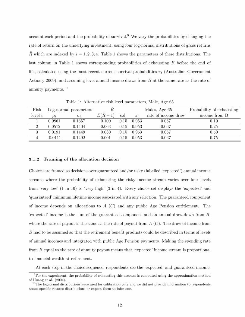
account each period and the probability of survival.9 We vary the probabilities by changing the

rate of return on the underlying investment, using four log-normal distributions of gross returns

R which are indexed by i = 1, 2, 3, 4. Table 1 shows the parameters of these distributions. The

last column in Table 1 shows corresponding probabilities of exhausting B before the end of

life, calculated using the most recent current survival probabilities πt (Australian Government

Actuary 2009), and assuming level annual income draws from B at the same rate as the rate of

annuity payments.10

Table 1: Alternative risk level parameters, Male, Age 65

Risk Log-normal parameters R Males, Age 65 Probability of exhausting

level i µi σi E(R− 1) s.d. πt rate of income draw income from B

1 0.0861 0.1357 0.100 0.15 0.953 0.067 0.10

2 0.0512 0.1404 0.063 0.15 0.953 0.067 0.25

3 0.0191 0.1449 0.030 0.15 0.953 0.067 0.50

4 -0.0111 0.1492 0.001 0.15 0.953 0.067 0.75

3.1.2 Framing of the allocation decision

Choices are framed as decisions over guaranteed and/or risky (labelled ‘expected’) annual income

streams where the probability of exhausting the risky income stream varies over four levels

from ‘very low’ (1 in 10) to ‘very high’ (3 in 4). Every choice set displays the ‘expected’ and

‘guaranteed’ minimum lifetime income associated with any selection. The guaranteed component

of income depends on allocations to A (C) and any public Age Pension entitlement. The

‘expected’ income is the sum of the guaranteed component and an annual draw-down from B,

where the rate of payout is the same as the rate of payout from A (C). The draw of income from

B had to be assumed so that the retirement benefit products could be described in terms of levels

of annual incomes and integrated with public Age Pension payments. Making the spending rate

from B equal to the rate of annuity payout means that ‘expected’ income stream is proportional

to financial wealth at retirement.

At each step in the choice sequence, respondents see the ‘expected’ and guaranteed income,

9For the experiment, the probability of exhausting this account is computed using the approximation methodof Huang et al. (2004).

10The lognormal distributions were used for calibration only and we did not provide information to respondentsabout specific returns distributions or expect them to infer one.

12

and the liquid wealth available for contingencies or unintentional bequest implied by their al-

location. However in each step of the sequence, the risk of a permanently lower income rises.

On seeing an increasing probability of exhausting the phased withdrawal account at the same

expected income, and hence an increasing risk of falling to a lower lifetime income, individuals

should allocate no more to B. The analysis in Section 4 evaluates whether each respondent’s se-

quence of percentage allocations to B do not increase as the risk of exhausting income from that

product rises. We label sequences of allocations that conform to this criterion as ‘consistent’.

3.1.3 Experiment instructions and design

The experiment section of the on-line survey begins with instructions, reproduced in Appendix

B, that set out a simplified retirement income plan. Respondents were asked to allocate their

retirement wealth (observed elsewhere in the survey) using what is known as a ‘product configu-

rator’ (e.g., Kamis, Koufaris and Stern, 2008), a slider that was manipulated by the respondent’s

cursor.

The experiment used a within and between subjects design. Subjects were sorted into 16

treatments groups: first by gender (2 groups), since annuity payments are lower for women

than for men because of longer life expectancy; second by predictions of financial wealth at

retirement (based on self-reported net worth), to allow for public Age Pension means-testing

(4 groups: $50K; $125K; $250K; $1 million) and to ensure that the task did not deviate too

much from experience; and finally by intended retirement age (2 groups: guaranteed incomes

of those retiring before public pension eligibility age did not include Age Pension payments).

Each participant then allocated their predicted retirement wealth in eight settings, the Cartesian

product of the four risk levels indicated in Table 1 and two pairs of products, A v. B and C v.

B.

Before they saw the choice sets, respondents read descriptions of products in terms of five

common features, Who provides this product?; How much income will I receive?; How long do

payments last?; What happens if I die? and Can I withdraw a lump sum for unforeseen events

or changes of plans? 11 Commercial product names were never mentioned. After viewing three

11We adapted wording from the Australian Securities and Investment Commission Mon-eySmart website https://www.moneysmart.gov.au/\penalty\z@superannuation-and-retirement/

\penalty\z@income-sources-in-retirement/\penalty\z@income-from-super/annuities and

13

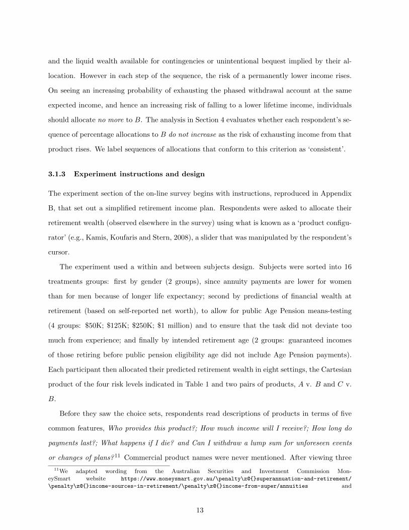
example choice sets, respondents were able to explore the continuum of product combinations by

clicking on the configurator, monitoring changes in expected and guaranteed income and access

to liquidity at different allocation weights, before making a final choice. A 50:50 allocation was

the default position of the configurator slider in all settings. Each choice scenario also showed

the probability that income from the phased withdrawal B would be exhausted before the end

of life, over four levels. Figure 2 illustrates a choice set at the lowest probability of exhausting

income from B.

Table 2 displays the expected and guaranteed incomes for a 25%, 50% and 75% allocation to

B for Males with and without the public Age Pension. Guaranteed income levels are comprised

of the fairly priced annuity stream ‘purchased’ at each allocation and any public Age Pension

for which the respondent was eligible. For example, a fairly priced life annuity for a 60 year old

male, (improved life expectancy of 88.64 years) pays $5.84 p.a. for each $100 of wealth allocated.

If 50% of a $50,000 retirement accumulation is allocated to the life annuity A, guaranteed income

without the Age Pension is $1,460 p.a. which explains the entry in row 3, column 5 of Table 1.

Expected income is the sum of the $1,460 income from A and another $1,460 from the allocation

of remaining wealth to B. The income amount for B assumes that income is withdrawn at a

rate equal to the annuity payout, that is at 5.84% p.a. of the wealth allocated to B.

3.2 Sample and survey context

We selected a random sample of 854 respondents from those members of the PureProfile online

panel of over 600,000 Australians who had at least one current pension plan account, were

between the ages of 50 and 64 in 2011 and who satisfied the residency requirements for the public

Age Pension. Under Australia’s Superannuation Guarantee, almost all workers between 18 and

65 years of age participate in the mandatory retirement savings system, mostly as members of

DC, privately managed, funds. Benefits are preserved until at least age 55 (rising to age 60 for

many in our sample) at which time plan members must decide how to use their accumulations.

Retirees who purchase income stream products accrue tax concessions over those who take lump

sum payments, and approximately half of preserved savings are transferred to income streams

https://www.moneysmart.gov.au/\penalty\z@superannuation-and-retirement/\penalty\z@

income-sources-in-retirement/\penalty\z@income-from-super/annuities.

14

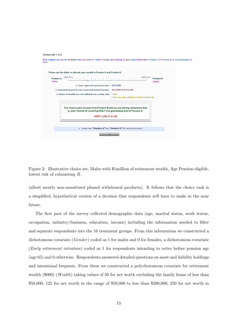
Figure 2: Illustrative choice set, Males with $1million of retirement wealth, Age Pension eligible,lowest risk of exhausting B.

(albeit mostly non-annuitized phased withdrawal products). It follows that the choice task is

a simplified, hypothetical version of a decision that respondents will have to make in the near

future.

The first part of the survey collected demographic data (age, marital status, work status,

occupation, industry/business, education, income) including the information needed to filter

and separate respondents into the 16 treatment groups. From this information we constructed a

dichotomous covariate (Gender) coded as 1 for males and 0 for females, a dichotomous covariate

(Early retirement intention) coded as 1 for respondents intending to retire before pension age

(age 65) and 0 otherwise. Respondents answered detailed questions on asset and liability holdings

and intentional bequests. From these we constructed a polychotomous covariate for retirement

wealth ($000) (Wealth) taking values of 50 for net worth excluding the family home of less than

$50,000, 125 for net worth in the range of $50,000 to less than $200,000, 250 for net worth in

15

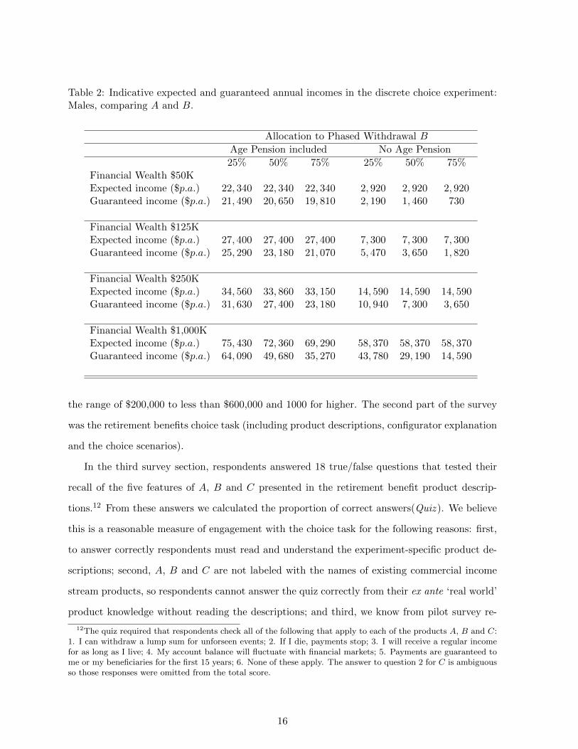
Table 2: Indicative expected and guaranteed annual incomes in the discrete choice experiment:Males, comparing A and B.

Allocation to Phased Withdrawal B

Age Pension included No Age Pension

25% 50% 75% 25% 50% 75%Financial Wealth $50KExpected income ($p.a.) 22, 340 22, 340 22, 340 2, 920 2, 920 2, 920Guaranteed income ($p.a.) 21, 490 20, 650 19, 810 2, 190 1, 460 730

Financial Wealth $125KExpected income ($p.a.) 27, 400 27, 400 27, 400 7, 300 7, 300 7, 300Guaranteed income ($p.a.) 25, 290 23, 180 21, 070 5, 470 3, 650 1, 820

Financial Wealth $250KExpected income ($p.a.) 34, 560 33, 860 33, 150 14, 590 14, 590 14, 590Guaranteed income ($p.a.) 31, 630 27, 400 23, 180 10, 940 7, 300 3, 650

Financial Wealth $1,000KExpected income ($p.a.) 75, 430 72, 360 69, 290 58, 370 58, 370 58, 370Guaranteed income ($p.a.) 64, 090 49, 680 35, 270 43, 780 29, 190 14, 590

the range of $200,000 to less than $600,000 and 1000 for higher. The second part of the survey

was the retirement benefits choice task (including product descriptions, configurator explanation

and the choice scenarios).

In the third survey section, respondents answered 18 true/false questions that tested their

recall of the five features of A, B and C presented in the retirement benefit product descrip-

tions.12 From these answers we calculated the proportion of correct answers(Quiz ). We believe

this is a reasonable measure of engagement with the choice task for the following reasons: first,

to answer correctly respondents must read and understand the experiment-specific product de-

scriptions; second, A, B and C are not labeled with the names of existing commercial income

stream products, so respondents cannot answer the quiz correctly from their ex ante ‘real world’

product knowledge without reading the descriptions; and third, we know from pilot survey re-

12The quiz required that respondents check all of the following that apply to each of the products A, B and C:1. I can withdraw a lump sum for unforseen events; 2. If I die, payments stop; 3. I will receive a regular incomefor as long as I live; 4. My account balance will fluctuate with financial markets; 5. Payments are guaranteed tome or my beneficiaries for the first 15 years; 6. None of these apply. The answer to question 2 for C is ambiguousso those responses were omitted from the total score.

16

sponses that awareness of retirement benefit products is very low.13 In Section 4 we show that

not paying attention to the descriptions of A, B and C makes consistent choices less likely.

Following the recall quiz, respondents answered questions on retirement planning and expec-

tations, bequest intentions, precautionary savings intentions, plans to liquidate housing wealth,

mortality and morbidity expectations and current quality of life. The questions from this section

that are included our final model are detailed in Appendix C. From these answers we constructed

a continuous covariate (Subjective life expectancy) measuring the deviation of the respondent’s

subjective life expectancy from that predicted by the Australian Life Tables. Positive values

indicate optimistic subjective survival expectations. We also constructed a polychotomous co-

variate for the financial aspects of retirement planning (Retirement financial planning) taking

the values 0, 1, 2, ..., 6 as the level of planning increased from ‘I haven’t thought at all about

what I will need for retirement’ to ‘I have a firm idea of what I need and I’m on track to reach

it’. As well we computed each respondent’s mean score across the five dimensions of quality of

life (mobility, self care, usual activities, pain and anxiety/depression) where 1 is very low and 3

is very high quality (Quality of Life).

The final part of the survey consists of questions measuring numeracy and financial literacy

skills, as well as self-assessed knowledge of finance, use of financial advice, trust in financial

service providers and awareness and knowledge of existing retirement income products.14 We

construct covariates (Numeracy, Basic Literacy and Sophisticated Literacy) as the proportion

of correct responses to each group of questions. Self-assessed financial literacy (Self-assessed

Literacy) is measured on a scale of 1-7 with 7 meaning very high understanding. Finally, we

create a covariate (Commercial product knowledge) as the proportion of correct answers in a

set of questions testing awareness of and detailed knowledge of real world retirement income

products. (See Appendix C.)

13Other possible proxies for task engagement, such as the number of times respondents ‘clicked’ to explore theconfigurator or the time spent completing the task, are likely to be noisier measures. For example, a person whounderstands products A and B well, perceives the risk of ruin accurately and who sees the income information mayclick few times on the allocation scale, having clear preferences. Similarly, time can be confounded by randomdistractions. Our recall quiz is similar to the Instructional Manipulation Check (IMC) of Oppenheimer et al.(2009), where satisficing survey participants who are not following instructions are identified.

14The three numeracy questions and four financial literacy questions, detailed in Appendix B, are drawn fromLipkus et al. (2001) and Lusardi and Mitchell (2009). Numeracy questions test proportions, percentages andsimple probability; two basic financial literacy questions test interest and inflation and two sophisticated financialliteracy questions test diversification.

17

From this information we selected numeracy, tested and subjectively assessed financial liter-

acy, product knowledge, current quality of life, subjective survival expectations, financial aspects

of retirement planning and the treatment indicators (gender, wealth and retirement intentions)

as covariates in the model to be discussed in Section 4. The selection was based on preliminary

estimations confirming that other potentially important covariates including age, formal educa-

tion, marital status, occupation, health expectations, bequest intentions, precautionary savings

intentions, detailed knowledge of the public pension and plans to leave the workforce, were not

relevant.

4 Econometric model and findings

We investigate the rate at which respondents choose consistently with standard expected utility

model predictions, as a function of task engagement and the covariates just described. The 854

complete responses are made up of four allocations between products A and B and four between

C and B, making 6, 832 in total. The first panel in Table 3 shows the average percentage

allocation to phased withdrawal B over life annuity A for each of the 16 treatment groups as

the risk of exhausting B rose from ‘very low’ to ‘very high’. The second panel shows average

percentage allocation to B over life annuity with guarantee, C.

18

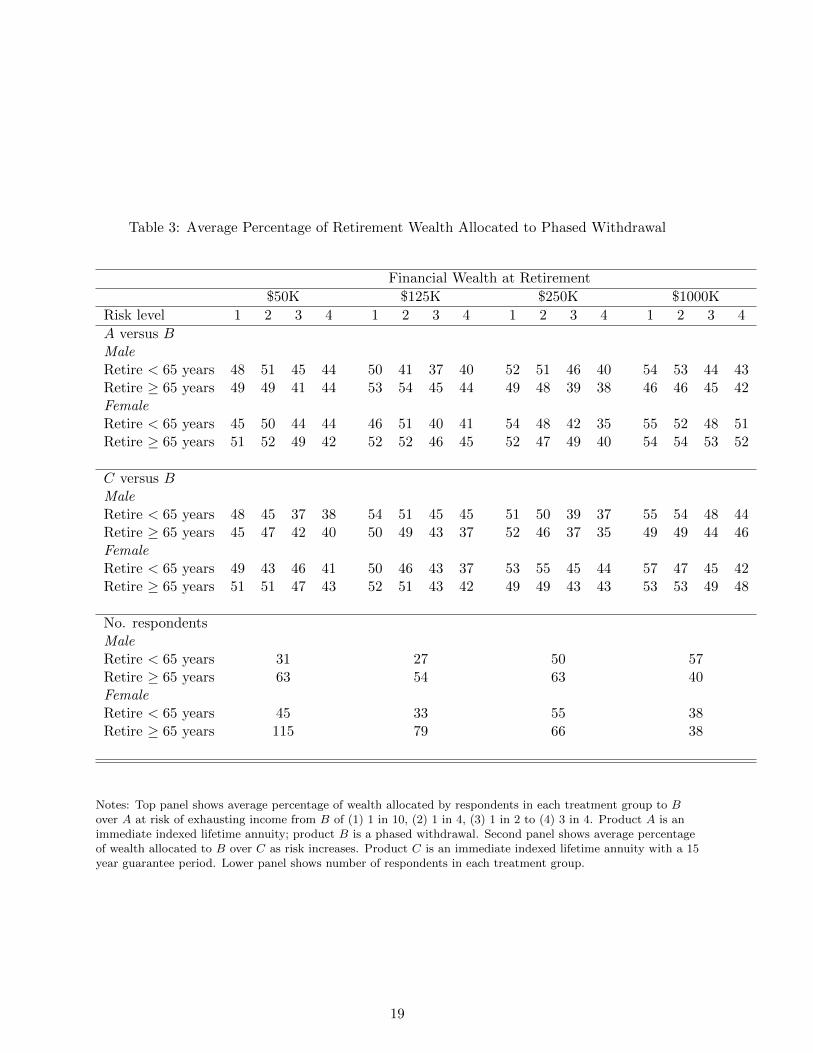
Table 3: Average Percentage of Retirement Wealth Allocated to Phased Withdrawal

Financial Wealth at Retirement

$50K $125K $250K $1000K

Risk level 1 2 3 4 1 2 3 4 1 2 3 4 1 2 3 4

A versus BMaleRetire < 65 years 48 51 45 44 50 41 37 40 52 51 46 40 54 53 44 43Retire ≥ 65 years 49 49 41 44 53 54 45 44 49 48 39 38 46 46 45 42FemaleRetire < 65 years 45 50 44 44 46 51 40 41 54 48 42 35 55 52 48 51Retire ≥ 65 years 51 52 49 42 52 52 46 45 52 47 49 40 54 54 53 52

C versus BMaleRetire < 65 years 48 45 37 38 54 51 45 45 51 50 39 37 55 54 48 44Retire ≥ 65 years 45 47 42 40 50 49 43 37 52 46 37 35 49 49 44 46FemaleRetire < 65 years 49 43 46 41 50 46 43 37 53 55 45 44 57 47 45 42Retire ≥ 65 years 51 51 47 43 52 51 43 42 49 49 43 43 53 53 49 48

No. respondentsMaleRetire < 65 years 31 27 50 57Retire ≥ 65 years 63 54 63 40FemaleRetire < 65 years 45 33 55 38Retire ≥ 65 years 115 79 66 38

Notes: Top panel shows average percentage of wealth allocated by respondents in each treatment group to Bover A at risk of exhausting income from B of (1) 1 in 10, (2) 1 in 4, (3) 1 in 2 to (4) 3 in 4. Product A is animmediate indexed lifetime annuity; product B is a phased withdrawal. Second panel shows average percentageof wealth allocated to B over C as risk increases. Product C is an immediate indexed lifetime annuity with a 15year guarantee period. Lower panel shows number of respondents in each treatment group.

19

Table 3 shows generally decreasing average allocations to B as risk rises, consistent with risk

aversion. Declines are more regular for the early retirement treatment groups (Retire < 65). For

these respondents, choice set displays of ‘guaranteed incomes’ did not include the public Age

Pension and consequently income reductions due to exhausting B were more conspicuous.

4.1 Inconsistency rates

We assume independence across respondents in the analysis. Each respondent r makes an

allocation to A and B (C and B) at each risk level i = 1, 2, 3, 4. We index the pairwise product

comparisons as f = 1, 2. For each respondent r, decisions over risk levels i in comparison sets f

result in two 4× 1 vectors of allocations to product B. If these vectors are non-increasing in the

percentage allocated to B as i rises, the respondent recognizes increasing risk and conforms with

our simple CRRA utility model. Respondents who do not conform may be missing or ignoring

one main benefit of purchasing an annuity. We treat the dichotomous outcome of violating

this condition as a random variable where P (v(f)r = 1) = p(f), for f = 1, 2. We label this the

independent response (IR) model.

The first column of Table 4 presents the estimates of p(f) for all respondents using only

counts of consistency: around one half of respondents increased their allocation to the phased

withdrawal (product B) as risk increased in both the A v.B and C v. B allocation tasks (the

weak condition). However, the condition that respondents choose a non-increasing percentage

allocation to B does not rule out respondents who always choose 50:50 allocations. The second

column of Table 4 presents estimates of p(f) where v(f)r = 1 is assigned to respondents who violate

the condition or who do not move the slider away from the default at all (the strong condition).

The standard error of each element in Table 4 is about 0.017 so the rates of inconsistency at

f = 2 are significantly lower than at f = 1. Respondents may have become more familiar with

the experimental task in the second round of choices and consequently made fewer errors. They

may also have preferred C to A.

In complex financial choices attentiveness and engagement are critical. Subjects bring their

own personal financial capability, expectations and other demographic characteristics to the

choice experiment. Of these, gender, wealth and retirement intentions are used here to sort

respondents into treatment groups. During the task, respondents will also be more or less

20

Table 4: Probabilities of inconsistent allocation sequences in sets A−B and C −B

Weak condition Strong condition

p(1) 0.555 0.717

p(2) 0.484 0.645

Note: Table shows estimate of IR probability of inconsistent allocations. The weak condition for conformity issatisfied where the percentage of wealth allocated to B never increases as i rises. The strong condition adds therequirement that respondents move the slider at least once, either to explore the choice set or make an allocation.

engaged, attending to instructions and information, maintaining attention and thinking through

the choices with varying intensities. Pre-determined financial capability could influence choices

both directly and indirectly: directly by enabling ‘consistent’ choice and indirectly by motivating

task engagement which then promotes consistent choices. Engagement is likely to be affected

by capability but is also endogenous to the choice task itself and hence potentially a predictor

of inconsistency.

We propose a triangular structure to model choices. The structure has two components:

the first determines endogenous task engagement conditional on a vector of pre-determined re-

spondent characteristics and the second estimates the probability of inconsistency conditional

on the vector of pre-determined characteristics and the measure of endogenous task engage-

ment. We call this the conditionally independent response model (CIR) where the probability

of inconsistent choices is independent of r and f but conditional on treatments and covariates.

We estimate the following recursive system of equations:

Quizr = β′1xr + εr (4)

Pr(vr = 1) = Λ(β′2xr + ψQuizr) (5)

Λ(z) =exp(z)

1 + exp(z)

where Quizr is the proportion of the recall quiz questions answered correctly by respondent r

(i.e., our measure of task engagement); xr is a vector of pre-determined variables measuring

numeracy, financial product knowledge, financial literacy, subjective financial understanding,

retirement finance planning, subjective life expectancy, quality of life, and treatment group

21

variables including gender, intended retirement age and wealth; and εr is an independent error

term.15

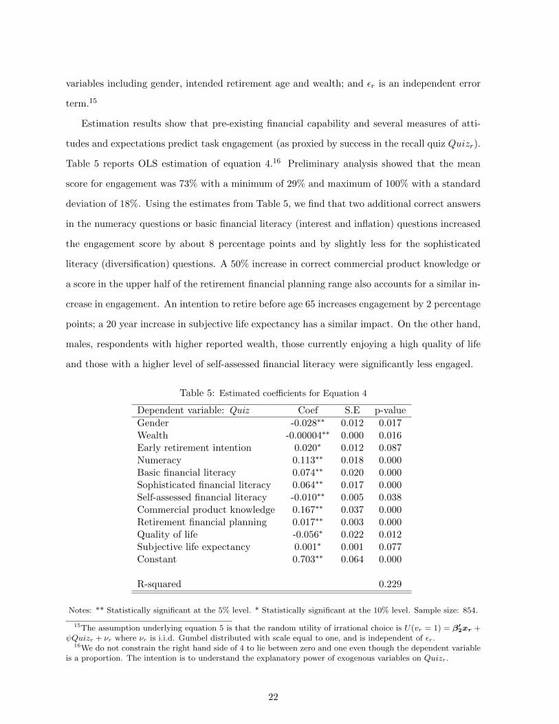
Estimation results show that pre-existing financial capability and several measures of atti-

tudes and expectations predict task engagement (as proxied by success in the recall quiz Quizr).

Table 5 reports OLS estimation of equation 4.16 Preliminary analysis showed that the mean

score for engagement was 73% with a minimum of 29% and maximum of 100% with a standard

deviation of 18%. Using the estimates from Table 5, we find that two additional correct answers

in the numeracy questions or basic financial literacy (interest and inflation) questions increased

the engagement score by about 8 percentage points and by slightly less for the sophisticated

literacy (diversification) questions. A 50% increase in correct commercial product knowledge or

a score in the upper half of the retirement financial planning range also accounts for a similar in-

crease in engagement. An intention to retire before age 65 increases engagement by 2 percentage

points; a 20 year increase in subjective life expectancy has a similar impact. On the other hand,

males, respondents with higher reported wealth, those currently enjoying a high quality of life

and those with a higher level of self-assessed financial literacy were significantly less engaged.

Table 5: Estimated coefficients for Equation 4

Dependent variable: Quiz Coef S.E p-value

Gender -0.028∗∗ 0.012 0.017Wealth -0.00004∗∗ 0.000 0.016Early retirement intention 0.020∗ 0.012 0.087Numeracy 0.113∗∗ 0.018 0.000Basic financial literacy 0.074∗∗ 0.020 0.000Sophisticated financial literacy 0.064∗∗ 0.017 0.000Self-assessed financial literacy -0.010∗∗ 0.005 0.038Commercial product knowledge 0.167∗∗ 0.037 0.000Retirement financial planning 0.017∗∗ 0.003 0.000Quality of life -0.056∗ 0.022 0.012Subjective life expectancy 0.001∗ 0.001 0.077Constant 0.703∗∗ 0.064 0.000

R-squared 0.229

Notes: ** Statistically significant at the 5% level. * Statistically significant at the 10% level. Sample size: 854.

15The assumption underlying equation 5 is that the random utility of irrational choice is U(vr = 1) = β′2xr +

ψQuizr + νr where νr is i.i.d. Gumbel distributed with scale equal to one, and is independent of εr.16We do not constrain the right hand side of 4 to lie between zero and one even though the dependent variable

is a proportion. The intention is to understand the explanatory power of exogenous variables on Quizr.

22

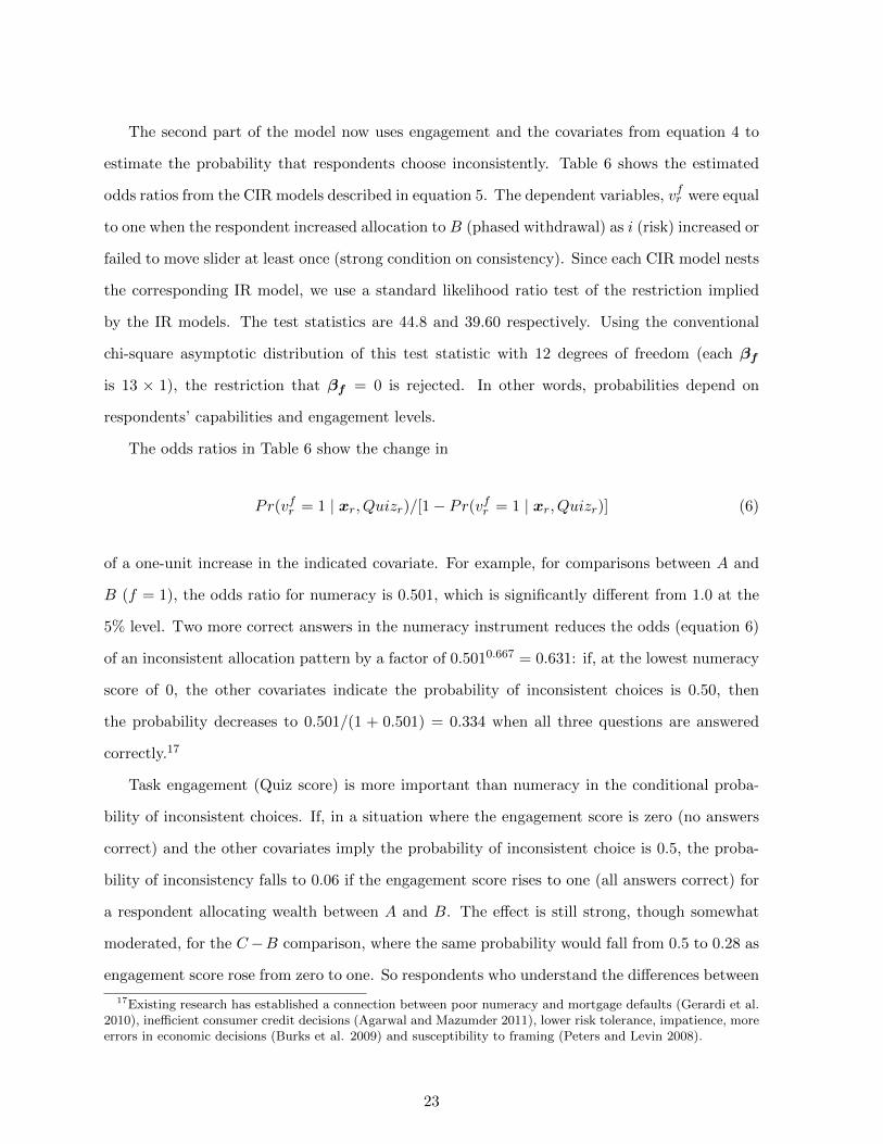
The second part of the model now uses engagement and the covariates from equation 4 to

estimate the probability that respondents choose inconsistently. Table 6 shows the estimated

odds ratios from the CIR models described in equation 5. The dependent variables, vfr were equal

to one when the respondent increased allocation to B (phased withdrawal) as i (risk) increased or

failed to move slider at least once (strong condition on consistency). Since each CIR model nests

the corresponding IR model, we use a standard likelihood ratio test of the restriction implied

by the IR models. The test statistics are 44.8 and 39.60 respectively. Using the conventional

chi-square asymptotic distribution of this test statistic with 12 degrees of freedom (each βf

is 13 × 1), the restriction that βf = 0 is rejected. In other words, probabilities depend on

respondents’ capabilities and engagement levels.

The odds ratios in Table 6 show the change in

Pr(vfr = 1 | xr, Quizr)/[1− Pr(vfr = 1 | xr, Quizr)] (6)

of a one-unit increase in the indicated covariate. For example, for comparisons between A and

B (f = 1), the odds ratio for numeracy is 0.501, which is significantly different from 1.0 at the

5% level. Two more correct answers in the numeracy instrument reduces the odds (equation 6)

of an inconsistent allocation pattern by a factor of 0.5010.667 = 0.631: if, at the lowest numeracy

score of 0, the other covariates indicate the probability of inconsistent choices is 0.50, then

the probability decreases to 0.501/(1 + 0.501) = 0.334 when all three questions are answered

correctly.17

Task engagement (Quiz score) is more important than numeracy in the conditional proba-

bility of inconsistent choices. If, in a situation where the engagement score is zero (no answers

correct) and the other covariates imply the probability of inconsistent choice is 0.5, the proba-

bility of inconsistency falls to 0.06 if the engagement score rises to one (all answers correct) for

a respondent allocating wealth between A and B. The effect is still strong, though somewhat

moderated, for the C−B comparison, where the same probability would fall from 0.5 to 0.28 as

engagement score rose from zero to one. So respondents who understand the differences between

17Existing research has established a connection between poor numeracy and mortgage defaults (Gerardi et al.2010), inefficient consumer credit decisions (Agarwal and Mazumder 2011), lower risk tolerance, impatience, moreerrors in economic decisions (Burks et al. 2009) and susceptibility to framing (Peters and Levin 2008).

23

the retirement products can make sound choices.

Surprisingly, other variables that were significant in equation 4 (i.e., financial literacy, com-

mercial product knowledge and retirement financial planning) are not directly relevant to in-

consistency rates. Only numeracy and task engagement are significant. To summarize, strong

financial literacy, general financial knowledge and a tendency to plan motivate individuals to

engage in the task, but it is a clear understanding of the specific features of the choice at hand,

and basic numerical ability, that ultimately drives consistent retirement benefit allocations.

Table 6: Estimated odds ratios for CIR equations 5

f = 1 f = 2

Quiz score 0.117∗∗ 0.401∗∗

Gender 1.154 0.796Wealth 1.000 1.000Early retirement intention 1.32 1.151Numeracy 0.501∗∗ 0.490∗∗

Basic financial literacy 1.312 1.115Sophisticated financial literacy 1.130 0.668Self-assessed financial literacy 0.993 1.019Retirement financial planning 0.952 0.938Quality of life 0.543 0.795Subjective life expectancy 1.001 0.998

Pseudo R2(McFadden) 0.044 0.036

Notes: Dependent variable vfr = 1 when respondent increased allocation to B (phased withdrawal) as i (risk)increased or failed to move slider at least once (strong condition on consistency). (1) is comparison A−B and(2) is comparison C −B. ** Statistically significant estimated coefficient at the 5% level. * Statisticallysignificant estimated coefficient at the 10% level. Sample size: 854.

Although the CIR model is more general than the IR model, it still imposes the restriction

that apart from the covariates included in the model, decisions over retirement income products

are independent between f = 1, 2. Under this restriction, collecting further details of individual’s

attitudes to investment and longevity risk would be unnecessary to anyone advising on retirement

financial planning. However, it is more likely that individual heterogeneity matters to decisions

beyond the inventory measured by model covariates so far.

We make a formal test of the restriction that unobserved individual heterogeneity is unim-

portant to consistency, within the limits of the current model, by generalizing the CIR model

24

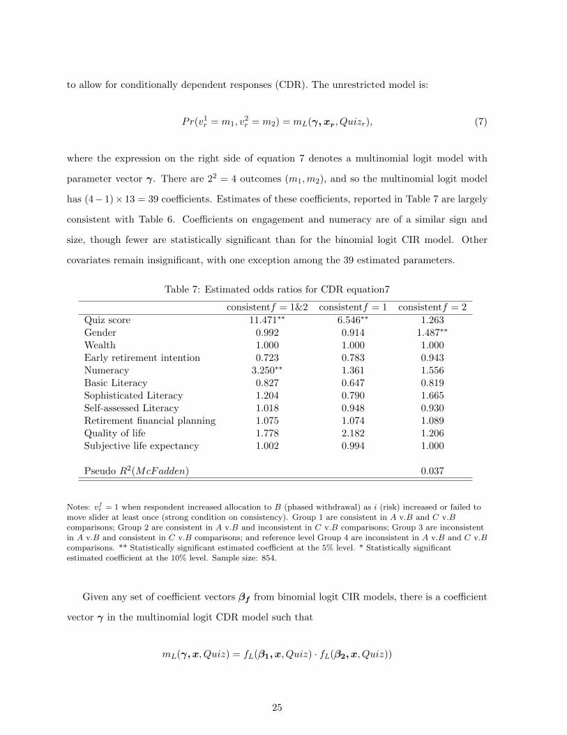
to allow for conditionally dependent responses (CDR). The unrestricted model is:

Pr(v1r = m1, v2r = m2) = mL(γ, xr, Quizr), (7)

where the expression on the right side of equation 7 denotes a multinomial logit model with

parameter vector γ. There are 22 = 4 outcomes (m1,m2), and so the multinomial logit model

has (4− 1)× 13 = 39 coefficients. Estimates of these coefficients, reported in Table 7 are largely

consistent with Table 6. Coefficients on engagement and numeracy are of a similar sign and

size, though fewer are statistically significant than for the binomial logit CIR model. Other

covariates remain insignificant, with one exception among the 39 estimated parameters.

Table 7: Estimated odds ratios for CDR equation7

consistentf = 1&2 consistentf = 1 consistentf = 2

Quiz score 11.471∗∗ 6.546∗∗ 1.263Gender 0.992 0.914 1.487∗∗

Wealth 1.000 1.000 1.000Early retirement intention 0.723 0.783 0.943Numeracy 3.250∗∗ 1.361 1.556Basic Literacy 0.827 0.647 0.819Sophisticated Literacy 1.204 0.790 1.665Self-assessed Literacy 1.018 0.948 0.930Retirement financial planning 1.075 1.074 1.089Quality of life 1.778 2.182 1.206Subjective life expectancy 1.002 0.994 1.000

Pseudo R2(McFadden) 0.037

Notes: vfr = 1 when respondent increased allocation to B (phased withdrawal) as i (risk) increased or failed tomove slider at least once (strong condition on consistency). Group 1 are consistent in A v.B and C v.Bcomparisons; Group 2 are consistent in A v.B and inconsistent in C v.B comparisons; Group 3 are inconsistentin A v.B and consistent in C v.B comparisons; and reference level Group 4 are inconsistent in A v.B and C v.Bcomparisons. ** Statistically significant estimated coefficient at the 5% level. * Statistically significantestimated coefficient at the 10% level. Sample size: 854.

Given any set of coefficient vectors βf from binomial logit CIR models, there is a coefficient

vector γ in the multinomial logit CDR model such that

mL(γ,x, Quiz) = fL(β1, x, Quiz) · fL(β2, x, Quiz))

25

for all possible (x, Quiz). Since the CDR model nests the CIR model, the maximum of the log

likelihood function in the CDR model cannot be smaller than the sum of the maximums of the

log likelihood functions in the two corresponding CIR models. The sum of the log likelihoods of

the CIR models is -1022.3 compared with -981.89 for the CDR model implying a test statistic

of 80.81. Using the conventional chi-square asymptotic distribution of this test statistic with

13 degrees of freedom (γ is 39 × 1, each βf is 13 × 1), the hypothesis of independence across

the two choice scenarios is rejected. In other words, idiosyncratic variation is still important to

retirement benefit choice patterns even after allowing for an array of demographic and capability

measures.

5 Conclusion and discussion

This paper studies the behavior of individuals as they allocate retirement wealth between a life-

time annuity and a phased withdrawal. This is an increasingly prevalent, yet complex, decision

in a DC world where retirement savers bear responsibility to turn lump sum benefits into lifetime

income. Most existing research assumes that people know about retirement income products

and have a basic grasp of how they function. We investigate the impact of disengagement and

poor understanding of products on the quality of allocations. Specifically, we measure how well

retirement plan members manage an increasing risk of running out of liquid wealth before the

end of life: respondents who reduce their exposure to this rising risk by maintaining or increasing

annuitization turn out to be engaged respondents who know how the products work.

Our analysis of retirement benefit choices can be described as follows:

1. A large minority of respondents choose consistently with predictions of a simple CRRA

utility maximization model by not increasing allocations of retirement wealth to the phased

withdrawal product as the probability of exhausting it increases. The remainder increase

their allocation to the phased withdrawal product even in the face of an increasing proba-

bility of permanently reducing income before the end of life. Inconsistency rates are lower

where the phased withdrawal product is paired with the annuity with 15 year guarantee

than where the guarantee is absent.

26

2. Respondents with higher financial capability (numeracy, financial literacy, and commercial

product knowledge) pay more attention to new information about the retirement products

and recall that information better when tested (measured using a post task quiz). For ex-

ample, two additional correct responses in the numeracy or basic financial literacy (interest

and inflation) questions improve scores in a quiz on the annuity and phased withdrawal

products by about one standard deviation.

3. However, financial capability is only indirectly connected with consistent choices, with

only numeracy having a direct, positive impact on the likelihood of rational choices over

and above its indirect effect on engagement with the choice task.

4. Task engagement (and numeracy) increase the probability that subjects will choose in a

consistent manner: at maximum engagement (measured by the number of correct answers

in the post task recall quiz of product features), the probability of inconsistent choices

declines by 90% compared with a zero engagement score, while raising numeracy from

minimum to maximum scores reduces the probability of inconsistency by around 40%.

Therefore, while strong financial literacy, general financial knowledge and a tendency to

plan can motivate individuals to engage in the task, it is a clear understanding of the

specific features of the choice at hand and basic numerical ability that enables better

allocation decisions. However, tests of dependence indicate that unobserved individual

heterogeneity is also important.

Our findings have several implications for policy makers and providers of retirement income

products. First, while revealed preference data suggest people show scant interest in annuity

products, our allocation task shows much more interest when products are described by their

characteristics, rather than their commercial names. In the experiment described here, where

respondents are given descriptions of products in terms of five common features (but no product

names), a majority say that they would fully or partially annuitize their retirement accumulation.

Revealed preference data is often used by government to support inaction in policy development

and by the financial services industry to justify a lack of product innovation. Our study suggests

that both government and industry need to take more care to explain the key insurance features

of alternative retirement benefit products before dismissing then as not interesting to consumers.

27

Second, our study tests how financial competence (numeracy and financial literacy, and

commercial product knowledge) can help people understand reasonably simple retirement benefit

product information. We find that those with more competence are more engaged, and the more

engaged are more likely to make ‘better’ decisions. While we cannot unequivocally translate

‘engagement’ with the hypothetical task to ‘real world’ engagement with the retirement benefit

decision, our findings do suggest improving the financial skills and product knowledge of real

world retirement savers might help, as recommended in Lusardi and Mitchell (2011) and Clark

et al. (2011) among others. The challenge is how to improve ’real world’ financial literacy and

commercial product knowledge of retirement savers through both education and improved benefit

product information formats. Finally, an overall implication of this study is that disengagement

with the retirement benefit decision could provide a partial solution to the annuity puzzle.

28

References

Agarwal, S., Mazumder, B., 2010. Cognitive Abilities and Household Financial Decision Making.Federal Reserve Bank of Chicago Working Paper Series No 2010-16, Chicago, Illinois.

Agnew, J., Anderson, l., Gerlach, J.R., Szykman, L., 2008. Who Chooses Annuities? An Experi-mental Investigation of the Role of Gender, Framing, and Defaults. American Economic Review.98, 418-22.

Australian Government Actuary, 2009. Australian Life Tables, Canberra, ACT, Department ofTreasury.

Benartzi, S., Previtero, A., Thaler, R.H., 2012. Annuitization Puzzles. Journal of EconomicPerspectives. 25(4),143-164.

Bernheim, B.D., 2002. Taxation and Saving, in: Auerbach, A.J., Feldstein, M., (Eds.), Handbookof Public Economics, Elsevier, 3, pp. 1173-1249.

Bernheim, B.D., 1991. How Strong Are Bequest Motives? Evidence Based on Estimates of theDemand for Life Insurance and Annuities. The Journal of Political Economy. 99(5), 899-927.

Beshears, J., Choi, J.J., Laibson, D., Madrian, B.C., 2008. How are Preferences Revealed?Journal of Public Economics 92(8-9), 1787-1794.

Beshears, J., Choi, J.J., Laibson, D., Madrian, B.C., Zeldes, S.P., 2012. What Makes Annuiti-zation More Appealing? NBER Working Paper 18575.

Brown, J., Poterba, J., 2001. Joint Life Annuities and the Demand for Annuities for MarriedCouples. Journal of Risk and Insurance. 67(4), 527-553.

Brown, J.R., Kling, J.R., Mullainathan, S., Wrobel, M.V., 2008. Why Don’t People InsureLate-Life Consumption? A Framing Explanation of the Under-Annuitization Puzzle. AmericanEconomic Review. 98, 418-22.

Brown, J.R., 2008. Understanding the Role of Annuities in Retirement Planning, in: Lusardi,A., (Ed.), Overcoming the Saving Slump. University of Chicago Press, Chicago, IL, 178-206.

Brown, J.R., Kapteyn, A., Mitchell, O.S., 2011. Do Consumers Know How to Value Annuities?Complexity as a Barrier to Annuitization’. RAND Financial Literacy Center Working PaperWR-924-SSA.

Burks, S.V., Carpenter, J.P., Goette, L., Rustichini, A., 2009. Cognitive skills affect economicpreferences, strategic behavior, and job attachment. Proceedings of the National Association ofSciences, 106, 7745-7750.

Butler, M., Teppa, F., 2007. The Choice between an Annuity and a Lump Sum: Results fromSwiss Pension Funds. Journal of Public Economics. 91(10), 1944-1966.

Camerer, C., Hogarth, R., 1999. The Effects of Financial Incentives in Experiments: A Reviewand Capital-Labor Production Framework. Journal of Risk and Uncertainty. 19(1), 7-42.

Cappelletti, G., Guazarotti, G., Tommasino, P., 2011. What determines annuity demand atretirement? Bank of Italy Temi di Discussione Working Paper No. 805.

29

Carroll, C., 2006. The Method of Endogenous Gridpoints for solving Dynamic Stochastic Opti-mization Problems. Economics Letters. 91(3), 312-320.

Clark, R., Morrill, M., Allen, S., 2009. Employer Provided Retirement Planning Programs, in:Clark, R., Mitchell, O.S., (Eds.), Reorienting Retirement Risk Management. Oxford UniversityPress, Oxford, UK, pp. 36-64.

Clark, R., Morrill, M., Allen, S., 2011. Pension Plan Distributions: The Importance of FinancialLiteracy. in: Mitchell, O.S., Lusardi, A., (Eds.), Financial Literacy: Implications for RetirementSecurity and the Financial Marketplace, Oxford University Press, Oxford, UK.

Davidoff, T., Brown, J., Diamond, P., 2005. Annuities and Individual Welfare. American Eco-nomic Review. 95(5), 1573-1590.

Dushi, I., Webb, A., 2004. Household Annuitization Decisions: Simulations and Empirical Anal-yses. Journal of Pension Economics and Finance. 3(2), 109-143.

Employee Benefits Research Institute (EBRI)., 2011. EBRI Databook on Employee Benefits.http://www.ebri.org/publications/books/?fa=databook.

Gerardi, K., Goette, L., Meier, S., 2010. Financial Literacy and Subprime Mortgage Delinquency:Evidence from a Survey Matched to Administrative Data. Federal Reserve Bank of AtlantaWorking Paper Series No 2010-10.

Guiso, L., Jappelli, T., 2008. Financial Literacy and Portfolio Diversification. European Univer-sity Institute Working Paper, ECO 2008/31.

Gustman, A.L., Steinmeier, T.L., Tabatabai, N., 2012. Financial Knowledge and Financial Lit-eracy at the Household Level. American Economic Review. 102(3), 309-12.

Harmer, J., 2009. Pension Review Report, 27 February 2009, Commonwealth of Australia.

Horneff, W., Maurer, R., Mitchell, O.S., Dus, I., 2007. Money in Motion: Asset Allocationand Annuitization in Retirement. NBER Working Paper 12942, National Bureau of EconomicResearch, Cambridge, MA. http://www.nber.org/papers/w12942.

Hu Wei-Yin., Scott, J.S., 2007. Behavioural Obstacles to the Annuity Market. Financial AnalystsJournal. 63(6), 71-82.

Huang, H., Milevsky, M.A., Wang, J., 2004. Ruined Moments in your Life: How Good are theApproximations? Insurance: Mathematics and Economics, 34, 421-447.

Inkmann, J., Lopes, P., Michaelides, A., 2011. How Deep Is the Annuity Market ParticipationPuzzle? Review of Financial Studies 24(1), 279-319.

Kamis, A., Koufaris, M., Stern, T., 2008. Using an Attribute-based DSS for User-customizedProducts online: An Experimental Investigation. MIS Quarterly 32(1), 159-177.

Kingston, G., Thorp, S., 2005. Annuitization and Asset Allocation with HARA Utility. Journalof Pension Economics and Finance. 4(3), 225-248.

Lipkus, I.M., Samsa, G., Rimer, B.K., 2001. General Performance on a Numeracy Scale amongHighly Educated Samples. Medical Decision Making 21(1), 37-44.

30

Lusardi, A., Mitchell, O.S, 2009. How Ordinary Consumers Make Complex Economic Decisions:Financial Literacy and Retirement Readiness. NBER Working Paper w15350, National Bureauof Economic Research, Cambridge, MA.

Lusardi, A., Mitchell, O.S., 2011. Financial Literacy around the World: An Overview. Journalof Pension Economics and Finance. 10(4), 497-508.

Milevsky, M., Young, V., 2007. Annuitization and Asset Allocation. Journal of Economic Dy-namics and Control. 31(9), 3138-3177.

Mitchell, O.S., Piggott, J., Takayama, T., 2011. Turning Wealth into Lifetime Income: TheChallenge Ahead, in: Mitchell, O.S., Piggott, J., Takayama, N., (Eds.), Securing Lifelong Re-tirement Income: Global Annuity Markets and Policy, Oxford University Press, pp. 1-9.

Mitchell, O.S., Poterba, J.M., Warshawsky, M.J., Brown, J.R., 1999. New Evidence on theMoney’s Worth of Individual Annuities. American Economic Review. 89(5), 1299-1318.

Oppenheimer, D.M., Meyvis, T., Davidenko, N., 2009. Instructional Manipulation Checks: De-tecting Satisficing to Increase Statistical Power. Journal of Experimental Social Psychology. 45,867-872.

Peijnenburg, K., Nijman, T., Werker, B., 2010. Health Cost Risk and Optimal RetirementProvision: A Simple Rule for Annuity Demand. Pension Research Council Working Paper No.WPS 2010-08.

Peters, E., Levin, I.P., 2008. Dissecting the Risky-choice Framing Effect: Numeracy as anIndividual-difference Factor in Weighting Risky and Riskless Options. Judgement and DecisionMaking. 3, 435-448.

Plan For Life., 2012. The Pension and Annuity Market Research Report, Mt. Waverly, VIC:Plan For Life Actuaries and Researchers.

Turra, C., Mitchell, O.S., 2008. The Impact of Health Status and Out-of-Pocket Medical Expen-ditures on Annuity Valuation, in: Ameriks, J., Mitchell, O.S., (Eds.) Recalibrating RetirementSpending and Saving, Oxford University Press, Oxford, UK.

Yaari, M., 1965. Uncertain Lifetime, Life Insurance, and the Theory of the Consumer. Reviewof Economic Studies. 32, 137-150.

31

Appendix A

Age Pension regulations

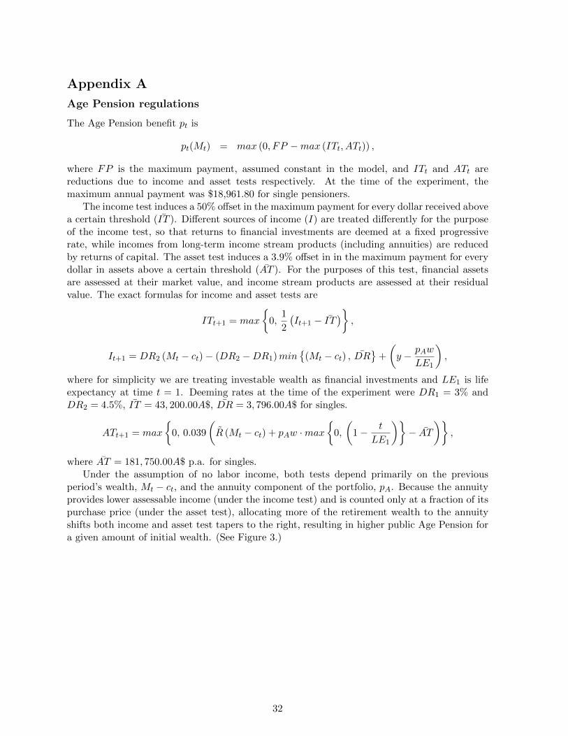
The Age Pension benefit pt is

pt(Mt) = max (0, FP −max (ITt, ATt)) ,

where FP is the maximum payment, assumed constant in the model, and ITt and ATt arereductions due to income and asset tests respectively. At the time of the experiment, themaximum annual payment was $18,961.80 for single pensioners.

The income test induces a 50% offset in the maximum payment for every dollar received abovea certain threshold (IT ). Different sources of income (I) are treated differently for the purposeof the income test, so that returns to financial investments are deemed at a fixed progressiverate, while incomes from long-term income stream products (including annuities) are reducedby returns of capital. The asset test induces a 3.9% offset in in the maximum payment for everydollar in assets above a certain threshold (AT ). For the purposes of this test, financial assetsare assessed at their market value, and income stream products are assessed at their residualvalue. The exact formulas for income and asset tests are

ITt+1 = max

0,

1

2

(It+1 − IT

),

It+1 = DR2 (Mt − ct)− (DR2 −DR1)min

(Mt − ct) , DR

+

(y − pAw

LE1

),

where for simplicity we are treating investable wealth as financial investments and LE1 is lifeexpectancy at time t = 1. Deeming rates at the time of the experiment were DR1 = 3% andDR2 = 4.5%, IT = 43, 200.00A$, DR = 3, 796.00A$ for singles.

ATt+1 = max

0, 0.039

(R (Mt − ct) + pAw ·max

0,

(1− t

LE1

)− AT

),

where AT = 181, 750.00A$ p.a. for singles.Under the assumption of no labor income, both tests depend primarily on the previous

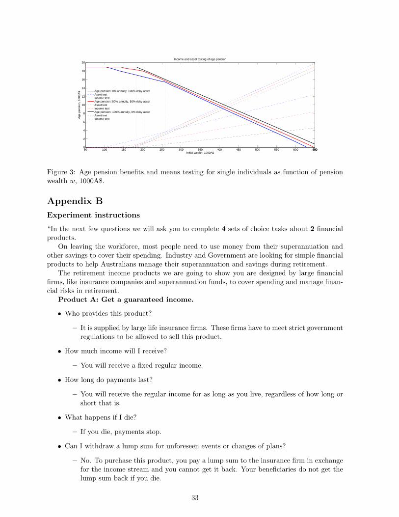
period’s wealth, Mt − ct, and the annuity component of the portfolio, pA. Because the annuityprovides lower assessable income (under the income test) and is counted only at a fraction of itspurchase price (under the asset test), allocating more of the retirement wealth to the annuityshifts both income and asset test tapers to the right, resulting in higher public Age Pension fora given amount of initial wealth. (See Figure 3.)

32

50 100 150 200 250 300 350 400 450 500 550 600 6506500

2

4

6

8

10

12

14

16

18

20

Initial wealth, 1000A$

Age

pen

sion

, 100

0A$

Income and asset testing of age pension

Age pension: 0% annuity, 100% risky assetAsset testIncome testAge pension: 50% annuity, 50% risky assetAsset testIncome testAge pension: 100% annuity, 0% risky assetAsset testIncome test

Figure 3: Age pension benefits and means testing for single individuals as function of pensionwealth w, 1000A$.

Appendix B

Experiment instructions

“In the next few questions we will ask you to complete 4 sets of choice tasks about 2 financialproducts.

On leaving the workforce, most people need to use money from their superannuation andother savings to cover their spending. Industry and Government are looking for simple financialproducts to help Australians manage their superannuation and savings during retirement.

The retirement income products we are going to show you are designed by large financialfirms, like insurance companies and superannuation funds, to cover spending and manage finan-cial risks in retirement.

Product A: Get a guaranteed income.

• Who provides this product?

– It is supplied by large life insurance firms. These firms have to meet strict governmentregulations to be allowed to sell this product.

• How much income will I receive?

– You will receive a fixed regular income.

• How long do payments last?

– You will receive the regular income for as long as you live, regardless of how long orshort that is.

• What happens if I die?

– If you die, payments stop.

• Can I withdraw a lump sum for unforeseen events or changes of plans?

– No. To purchase this product, you pay a lump sum to the insurance firm in exchangefor the income stream and you cannot get it back. Your beneficiaries do not get thelump sum back if you die.

33

Product B: Withdraw a regular income.

• Who provides this product?

– It is supplied by superannuation funds. Your money is held in an account and investedin financial assets like shares and bonds.

• How much income will I receive?

– You can decide how much of your balance to withdraw each year. Your accountbalance will fluctuate each year with financial markets. You will pay fees each yearto the fund that manages your account.

• How long do payments last?

– There is no guarantee you will have a lifetime income. How long payments lastdepends on investment returns, fees and your withdrawals.

• What happens if I die?

– If you die, remaining money in your account goes to your dependents or your estate.

• Can I withdraw a lump sum for unforeseen events or changes of plans?

– Yes. You can take all or a part of any remaining money out, but if you do it will notbe available to pay you income in the future.”

Respondents were then shown several examples of the product configurator and completedfour choices. After that they saw another screen: “Thank you for completing the last 4 tasks.Now we want you to compare Product B with a different type of guaranteed income product inanother 4 similar tasks.

Product C: Get a guaranteed income with a fixed term payment period.

• Who provides this product?

– It is supplied by large life insurance firms. These firms have to meet strict governmentregulations to be allowed to sell this product.

• How much income will I receive?

– You or your beneficiaries will receive a fixed regular income.

• How long do payments last?

– You personally will receive the regular income for as long as you live, regardless ofhow long or short that is. If you die within the fixed term period, the regular incomecontinues to be paid to your beneficiaries or estate up to the end of the 15th year.

• What happens if I die?

– Payments are guaranteed to you or your beneficiaries for the first 15 years, even ifyou die within that period. Payments are guaranteed only to you after that time.

• Can I withdraw a lump sum for unforeseen events or changes of plans?

– No. To purchase this product, you pay a lump sum to the insurance firm in exchangefor the income stream and you cannot get it back. Your beneficiaries do not get thelump sum back if you pass away.”

34

Appendix C

Life expectancy/current age:

• To what age do you think you will live?

• What is your current age?

Financial aspects of retirement planning question:

• Which of the following statements best describes your thoughts about the financial aspectsof retirement?

1. I haven’t thought at all about what I will need for retirement

2. I have just started to think about what I will need in terms of savings for retirement,but haven’t checked out my current financial position.

3. I have thought about it a fair bit, and have checked out my current financial position.

4. I have some firm ideas about what I will need and have compared my current positionwith my idea of what I will need.

5. I have a firm idea of what I need but I’m not sure if I can reach it, and haven‘tplanned a way to get there.

6. I have a firm idea of what I need, I’m not sure if I can reach it, but I have planned away to get there.

7. I have a firm idea of what I need and I’m on track to reach it.

Quality of Life questions:

• Mobility

1. I am confined to bed

2. I have SOME PROBLEMS walking around

3. I have NO PROBLEMS walking around

• Self-care

1. I CANNOT wash or dress myself

2. I have SOME PROBLEMS washing or dressing myself

3. I have NO PROBLEMS with self-care

• Activities

1. I CANNOT do my usual activities

2. I have SOME PROBLEMS doing my usual activities

3. I have NO PROBLEMS doing all my usual activities

• Pain/Discomfort

1. I have A LOT of pain or discomfort

2. I have MODERATE pain or discomfort

3. I have NO pain or discomfort

35

• Anxiety/Depression

1. I’m VERY anxious or depressed

2. I’m MODERATELY anxious or depressed

3. I’m NOT anxious or depressed

Self-assessed financial literacy

• On a scale of 1 to 7, where 1 means very low and 7 means very high, how would you assessyour understanding of finance?

Numeracy:

• Imagine that we rolled a fair, six-sided die 1,000 times. Out of 1,000 rolls, how many timesdo you think the die would come up with even numbers?

• In a lottery, the chance of winning a $10 prize is 1%. What is your best guess about howmany people would win a $10 price if 1,000 people each buy a single ticket to the lottery.

• In a raffle, the chance of winning a car is 1 in 1,000. What percent of tickets in the rafflewin a car?

Financial Literacy:

• Suppose you had $100 in a savings account and the interest rate was 2% per year. After5 years how much do you think you would have in the account if you left the money togrow?

• Imagine that the interest rate on your savings account was 1% per year and inflation was2% per year. After 1 year, how much would you be able to buy with the money in thisaccount?

• When an investor spreads his money among different assets, does the risk of losing money?

• Please tell me whether this statement is true or false. ‘Buying a single company’s sharesusually provides a safer return than a share managed fund.’

Commercial product knowledgeRespondents were asked the following:Below is a list of features for products. For each product listed..., please select all product

features that you think apply to each product. Please select all that apply for each product... thatyou have heard of.

The products surveyed were:

• Allocated (or account-based) pension

• Lifetime annuity

• Term certain annuity

• CPI Indexed lifetime annuity

• Single lifetime annuity with reversion

36

• Guaranteed lifetime annuity

• Transition to retirement pension

• None of these

The features surveyed were:

• To purchase this product, I pay a lump sum of my capital and do not get it back.

• My capital is tied up for a fixed term.

• My account balance will go up and down with the financial markets.

• I can choose the amount of income I withdraw, as long as I withdraw the minimum requiredby the government.

• I can withdraw my capital/ balance at any time or leave it to someone in my will.

• The dollar amount of my capital is guaranteed not to go down.

• I can choose where my money is invested.

• The dollar amount of my income is guaranteed not to go down.

• My income is guaranteed to increase with inflation.

• The value of my capital is guaranteed to increase with inflation.

• Income from this product lasts my whole life regardless of how long I live.

• If I die, my partner can receive the income from this product.

• If I die, my partner or beneficiaries can receive the capital/balance from this product.

Consistency definitions used are:

1. Non-increasing allocation to the phased withdrawal product B for all four choices in Aversus B and move the slider at least once (1).

2. Non-increasing allocation to the phased withdrawal product B for all four choices in Cversus B and move the slider at least once (2).

37