Diseconomies of Scale in Employment Contracts

August 14, 1992

Eric Rasmusen and Todd Zenger

Published: Journal of Law, Economics and Organization (June 1990), 6:65-92 Abstract

We �nd that small teams can write more e�cient incentive contracts thanlarge teams when agents choose individual e�ort levels but the principalobserves only the joint output. This result is helpful in understanding orga-nizational diseconomies of scale and is consistent with both existing evidenceand our own analysis of data from the Current Population Survey. Our mod-elling approach, similar to classical hypothesis testing, is of interest becausewe need not derive the optimal contract to show the advantage of smallteams.

Rasmusen: John M. Olin Visiting Assistant Professor, Center for the Study

of the Economy and the State and Graduate School of Business, University of

Chicago 60637, and UCLA AGSM. Phone: (312) 702-9478. Fax: (312) 702-0458.

Bitnet: Fac ras@gsbacd.uchicago.edu.

Zenger: School of Business and Management, Pepperdine University, 3rd oor,

400 Corporate Point, Culver City, Cal. 90230. Phone: (714) 941-0329. Fax: 213-

568-5727.

2000: Eric Rasmusen, Professor of Business Economics and Public Pol-icy and Sanjay Subhedar Faculty Fellow, Indiana University, Kelley School

of Business, BU 456, 1309 E 10th Street, Bloomington, Indiana, 47405-1701. O�ce: (812) 855-9219. Fax: 812-855-3354. Erasmuse@indiana.edu.Php.indiana.edu/�erasmuse.

1

I. Introduction.

The Problem of Firm Size.

A central question in industrial organization is what determines the sizeof �rms. This question is closely linked to a central assumption in microe-conomics generally: that \managerial diseconomies of scale" limit the sizeof �rms. If such diseconomies of scale did not exist, many industries wouldbe natural monopolies, because average cost declines with output for anytechnology with a �xed cost and constant marginal cost. This was notedby Sra�a (1926) and Kaldor (1934), who concluded that perfect competitionwas unrealistic. Modern textbook theory, rejecting the premise of constantmarginal cost, notes that if marginal cost rises with output, then a large �rmis ine�cient and a competitive market is feasible. The combination of risingmarginal cost and a �xed cost generates the Vinerian U-shaped average costcurve, not natural monopoly.

The commonly given reason for increasing long-run marginal cost, a rea-son mentioned as far back as Kaldor (1934), is that a larger �rm is harderto manage. Why this should be so is not entirely clear. Indeed, Alfred Mar-shall believed that there were managerial economies of scale, which wouldaggravate the problem noted by Kaldor and Sra�a.1 Schumpeter also seemsto have believed in managerial economies of scale, because \monopolizationmay increase the sphere of in uence of the better, and decrease the sphere ofin uence of the inferior, brains."2 Modern casual empiricism, if not that ofAlfred Marshall, suggests that large organizations su�er from diseconomies.Not only is there no tendency towards monopoly in most unregulated mar-kets, but in most industries one observes a variety of �rm sizes.3 Coase (1937)has argued that optimal �rm size is determined by a comparative assessmentof the costs of internalizing additional transactions and the costs of mar-ket transactions. At some point the cost of organizing another transactionwithin the �rm becomes greater than the cost of transacting in the openmarket. But Coase merely provided a general framework, not a reason whytransactions costs should rise as the �rm becomes larger. As he notes in a1988 article, why the marginal costs of internal organization should rise withincreased size remains unexplained.

2

Recently, several theorists have developed arguments to explain organiza-tional diseconomies of scale. Williamson (1985, Chapter 6) argues that com-mon ownership of successive stages of production, unlike separate ownership,creates incentives for managers governed by incentive contracts to misuti-lize assets and opportunistically manipulate accounting data. Consequently,joint ownership of successive production stages requires costly supplementalmonitoring to enforce incentive contracts. These enforcement costs and resid-ual opportunistic behavior render incentive contracts ine�cient, thereby dis-couraging joint ownership. Milgrom and Roberts (1988a,b) and Holmstrom(1988) argue that organizations, unlike markets, must contend with \in u-ence costs"| costs that arise whenever individuals try to in uence decisionsto their private bene�t and whenever organizations impose mechanisms tocontrol this behavior. But the above arguments, although helpful in speci-fying the costs of internal organization, do not address why these or othercosts of internal organization would necessarily increase with the size of the�rm.

Diseconomies of scale also arise in organizations other than �rms. Sug-den (1986, chapter 5) and, more formally, Boyd and Richerson (1988) �ndthat increasing the size of a group makes evolutionary development of aconvention| a coordination rule such as driving on the right| more di�cult.A convention works better when used more widely, and moving randomlyfrom discoordination to coordination is easier in a smaller group. Farrell andLander (1989) use a team model to look at the distinction between an indi-vidual's e�ort on his own behalf and on the team's behalf under certainty.They �nd for a particular contractual form that sel�sh e�ort increases andteam e�ort decreases in team size. More directly related to �rm size, RobertFrank (1985) in Choosing the Right Pond argues that if managers are willingto sacri�ce monetary compensation in exchange for being top man in their�rms, then small �rms could outcompete large �rms.

Bendor & Mookherjee (1987) analyze the e�ect of group size on cooper-ation in an in�nitely repeated Prisoner's Dilemma. They note that as thegroup size becomes larger, the free rider problem increases. For a given dis-count rate, cooperation cannot be supported beyond a critical group size thatdepends on the discount rate. This has the same avor as work on the size ofcartels, such as Stigler's 1964 model of a cartel that tries to detect cheaters

3

using a noisy variable whose mean depends on whether cheating occurs. Inhis model, a �rm only knows how many customers do not return to it, so each�rm sees a di�erent statistic. As the number of �rms increases, detecting aprice-cutter becomes more di�cult. The problem has been taken up againin the \trigger strategy" literature, where detection triggers dissolution ofthe cartel. Porter (1983) comes to a result similar to Stigler's: a cartel withmore members has a shorter expected lifetime.

Our Approach.

We hope to shed some light on the issue of organizational diseconomiesof scale from a new viewpoint: thinking of the organization as a team ofagents who may di�er in e�ort or ability. We will show why teams incurdiseconomies of scale and why teams can coexist with di�erent managementstyles. Our argument will be that the small team can more e�ciently con-struct incentive contracts to induce high e�ort and attract talented workers,an argument that applies to any organization generating a joint output whenthe inputs of individual members are di�cult to assess.

We will use an agency model similar to Holmstrom (1982) in which totalteam output is observable but individual contributions are not. Holmstromfocuses on the manager's role in ensuring optimal e�ort. Even without amanager the team faces the di�culty of detecting low e�ort, but the man-ager's presence expands the space of contracts by enforcing drastic punish-ment if output is low. In a world of certainty this allows the �rst-best to beachieved. The Holmstrommodel by itself thus does not explain diseconomiesof scale; on the contrary, one may draw from it the surprising implicationthat a properly designed contract can avoid them.

We will assume that contracts are enforceable in that managers will al-ways impose the punishments stipulated by the contract, and focus insteadon team size under uncertainty, where low output might be due to randomnoise instead of shirking. The manager must still deter shirking by the threatof a teamwide punishment if output is below a chosen threshold. We will ex-amine the case where the optimal contract is costly: even if in icting thepunishment incurs deadweight loss, some mistaken punishment occurs be-cause of the noise, and the �rst-best cannot be achieved. We will show that

4

the costs associated with the optimal contract increase with team size. Thisresult will be obtained in a way that avoids the di�cult task of characterizingthe optimal contract. Our argument will apply both to moral hazard (whene�ort is variable) and adverse selection (when ability is variable). The impli-cation is that large teams must be content with low e�ort and ability or elseuse ability testing and e�ort monitoring instead of output-based contracts.

We believe that our results on teams are relevant to thinking about orga-nizational diseconomies of scale. In the case of small �rms, our results applydirectly, since the �rm may be nothing more than a small team of produc-tion workers. Large �rms, however, are commonly comprised not of one largeteam, but of many subunits. Despite this, it is relatively uncommon for anysigni�cant element of compensation to be explicitly tied to subunit output.Why don't large �rms simply replicate small-�rm incentives by attachingcompensation to subunit performance? Presumably, these subunits are notteams in our sense, with a clearly observable team output. Rather, the out-put of a subunit depends on the inputs of other subunits and management.Consequently, breaking into small subunits does not permit the large �rm toreplicate the contracting advantage of the small �rm.4

Our model also has application to management teams. It may well bethat the individual output of production workers is fully observable, but theboard of directors cannot distinguish the individual contributions of the top�ve executives. In this case, our model predicts that �rms with fewer topexecutives could construct contracts which attract greater talent at the exec-utive level. If the number of executives limits the size of the �rm, then onlyrelatively small �rms will employ high-ability executives and use incentivecontracts.

The teams approach is important because it complements an older idea:the �rm cannot simply replicate divisions, because it can have only one chiefexecutive, who runs into diminishing returns when used intensively. This isthe idea extended and modelled by the literature starting with Williamson(1967) and continuing in, for example, Keren and Levhari (1983) and McAfeeand McMillan (1989a). Williamson constructs a model with an exogenous\span of control," an exogenous ratio of agents to managers at each level ofthe �rm. Since managers are not directly productive, this assumption makes

5

average costs increase in output. The interesting questions in Williamson'spaper concern the optimal number of levels in the �rm hierarchy, however,rather than why large �rms are ine�cient, since the ine�ciency is a direct as-sumption about the management technology. The span-of-control approachasks how to optimize the �rm's structure given organizational diseconomiesof scale, but it does not inquire into their origins. Our paper suggests thatone reason for span-of-control problems is the increasing cost of extendingincentive contracts as span increases.

The single-executive explanation for why replication is ine�ective in re-moving managerial diseconomies of scale is satisfactory only if we take it forgranted that a �rm must have only one chief executive. But why not replacethe chief executive with a management team, increasing the number of exec-utives as the amount of necessary supervision increases? We will show thatusing a team is costly, and it is more costly the larger the team. Hence, mak-ing the management team larger by horizontal expansion of the hiearchy'stop level is not a costless substitute for increasing the number of hierarchicallevels by vertical expansion.

The teams approach may also explain why vertical expansion of the hi-erarchy with monitoring cannot be replaced by vertical incentive contracts.The individuals we model as a team need not be at the same hierarchicallevel. The reasoning applies even if one of the team members is a boss,whose ability is twice as high as an ordinary member and who is paid a dou-ble share, but whose e�ect on team output cannot be untangled from thee�ect of his subordinates. The results hold a fortiori, since low e�ort by theboss is as easy to detect as low e�ort by two ordinary members with perfectlycorrelated errors. All that is required is that the double importance of theboss is common knowledge. Thus, our model in its broadest interpretationsuggests that as the number of individuals contributing to an observable out-put increases, the costs of o�ering incentive contracts rise regardless of theindividuals' hiearchical location within the organization.

Sections II and III of this article present the model and show why contractcosts increase with team size. Section IV discusses the applicability of theresults to models of adverse selection, in which smaller �rms can o�er lower-cost contracts to attract high-ability agents while deterring the low-ability.

6

Section V lays out the empirical implications of the model and comparesthem with evidence from the 1979 Current Population Survey.

7

II. The Model.

A principal employs n agents to make up a team. The agents are iden-tical, with a utility function U(w; b; e) that is increasing in the wage w anddecreasing in the punishment b and the e�ort e. E�ort takes one of twolevels, qh or ql, where qh > ql. Agent i's contribution to output is the sumof his e�ort and a random disturbance:

qh = qh + "i or ql = ql + "i: (1)

The disturbances "i are identically distributed with mean zero accordingto a multivariate normal distribution, and they may be either independentor positively correlated. If the disturbances are independent, the randomin uence is at the level of the individual agent; if they are perfectly correlated,it is at the level of the team. We use the normal distribution so that totalteam output follows the same distribution regardless of team size. This allowsoutput to range from negative in�nity to positive in�nity, so some readersmay wish to interpret the variable as some other measure of performancebesides output (e.g. pro�t).

Competing teams o�er contracts to the agents, who choose the contractthat yields the greatest expected utility. After the agents choose contractsand e�orts, nature chooses the values of the disturbances and the team out-puts appear. The principals then pay or penalize the agents according to theterms of the contracts.

Individual e�ort and output are prohibitively costly for a principal to de-termine, so his contract must rely solely on the level of team output, denotedQobs. The principal is risk neutral and seeks to maximize pro�t, the expectedvalue of (Qobs � nw). The simplest kind of contract ignores Qobs and pays a�xed wage of w = ql, which elicits low e�ort and produce an expected pro�tof zero. If agents are su�ciently averse to risk and e�ort, this is the e�cientoutcome under asymmetric information| incentives for high e�ort are toocostly. We will assume the opposite|that high e�ort is more e�cient, evenunder asymmetric information| for the remainder of this article.

We will also assume that welfare under asymmetric information is not ashigh as it would be under full information| that is, the incentives necesssary

8

to induce high e�ort do generate costs. This is important because if neitherlarge nor small teams incur costs, there is no cost di�erence between them.The assumption that incentives are costly can be justi�ed by various com-binations of primitive assumptions. If incentives require variability, and theagents are risk averse, then any variability in wages is costly. If the agentsare risk neutral then wage variability does not matter, but if the principal isconstrained in the wage contracts he can write he may be forced to use dis-sipative penalties. But the agent's utility function will matter only becauseof the two requirements that (a) high e�ort is e�cient under asymmetricinformation, and (b) the asymmetry of information has no costless remedy.

The principal wishes to design a contract that supports a Nash equilib-rium in which every agent exerts high e�ort. Since behavior under the Nashequilibrium concept presumes that each player calculates whether his uni-lateral deviation from equilibrium behavior is pro�table, the willingness ofone or more agents to switch would break the equilibrium. The principal'sproblem is therefore to make it unpro�table for even a single agent to chooselow e�ort. If all n agents in a team choose high e�ort, output is the randomvariable

Qn;H =nX

i=1

(qh + "i); (2)

which is the equilibrium output. If all but one of the n agents choose highe�ort, output is the random variable

Qn;L = ql + "1 +nX

i=2

(qh + "i); (3)

which is the deviation output.

Testing for Shirkers.

Rather than directly attacking the problem of optimal contract design,we will start with the subproblem of detecting a low-e�ort agent. Underclassical hypothesis testing, we establish a null hypothesis,

\H0: All agents chose high e�ort, "

9

and an alternative hypothesis,

\H1: At least one agent chose low e�ort."

H1 is a little more general than is required here, since for Nash equilibriumall that is necessary is to test for one agent choosing low e�ort. A strategycombination is a Nash equilibrium if no player has any incentive to unilater-ally deviate from his strategy. In this case, all agents will choose high e�ortin the proposed equilibrium, so we must test to see whether a single agentcan bene�t by deviating and choosing low e�ort. Whether several playersmight bene�t by forming a coalition and simultaneously deviating is irrele-vant to whether the strategy combination is a Nash equilibrium. But in thisparticular model, the Nash equilibrium concept is not restrictive. A test thatdetects deviation by a single low-e�ort agent would even more easily detectdeviation by several agents who chose low e�ort simultaneously.

The principal is concerned with two types of errors:

Type I Error: Rejecting H0, when it should be accepted.(false rejection, associated with a low signi�cance level)

Type II Error: Accepting H0, when it should be rejected.(false acceptance, associated with low power)

The principal wishes to avoid both types of error. Equivalently, he wantsthe detection test to have high values for (1) its power (the probability thata low-e�ort agent will be detected when present) and (2) its signi�cance level(the probability of avoiding false detection).5 If the power is high, the �rm'sprobability of punishing a shirking agent is high and the agents fear to shirk.If the signi�cance level is high, false detection is rare and agents need not bepaid a large premium as compensation for expected accidental punishments.Both the power and the signi�cance level are determined by the particulartest.

Economists are used to trading o� the levels of desirable characteristics.Here, however, the principal just desires a power that deters shirking. Higherlevels of power are no better, so the lexicographic approach of classical hy-

10

pothesis testing is appropriate. The classical statistician chooses the signif-icance level for a test and then maximizes the power given that signi�cancelevel. Here, the principal chooses the test's power (to be high enough todeter shirking), and then maximizes the signi�cance level (which minimizesthe premium for accidental punishment).

We will concentrate on the simple test that uses only the informationof whether total output has exceeded a threshold level T . The principalaccepts (H0: All agents chose high e�ort) if Qobs � T and (H1: At leastone agent chose low e�ort) if Qobs < T . This test is illustrated by Figure 1.The signi�cance level of the test, S, is one minus the probability that theprincipal mistakenly believes that a single agent chose low e�ort:

S = 1� Prob(Qn;H � T ): (4)

The signi�cance level falls as the threshold rises:

dS

dT< 0: (5)

The power of the test, P , is the probability that a single shirking agent willbe detected when present:

P = Prob(Qn;L � T ): (6)

The power rises as the threshold rises:

dP

dT> 0: (7)

Figure 1: Power and Signi�cance Level

The characteristics of this test are well-known, for it is simply a test forthe mean of a normal distribution with known variance against a compos-ite alternative hypothesis. It is, in fact, a textbook example for power andsigni�cance level, and it provides the best critical region for testing our hy-pothesis. It is also the uniformly most powerful test: not only can it test forthe family of alternative hypotheses in which n agents shirk, it is the bestsuch test for all of those alternative hypotheses.6

11

The Compensation Contract.

A natural contract to associate with the threshold test consists of thetriplet (T;w; b). Each agent receives w if output exceeds the threshold T

and su�ers punishment b if output fails to exceed T . We have no reason tobelieve that the optimal contract lies within this restricted contract space,but as will be explained at the end of Section III, this is not so restrictive asit might seem.

Using the contract (T;w; b), the principal must choose threshold and pun-ishment values such that if the agent shirks, his expected utility is lower thanif he works. The expected utility of shirking is based on the probabilities of(a) being caught and rightfully punished (the power), and (b) successful de-ception and a wage of w. But the agent must compare the expected utilityof shirking not with a �xed utility from working hard, but with the expectedutility of working hard. The expected utility of working hard is based onthe probabilities of (a) being mistakenly punished, and (b) being paid w (thesigni�cance level).

The �rst requirement for a contract is that it deter shirking. Any of awide range of powers can succeed in this, since the punishment can be chosenappropriately to the power| a bigger punishment for a smaller power. Thesecond requirement for a contract is that it minimize the cost of mistakenpunishment. Thus, a high signi�cance level is desirable. But there is atradeo� between these two requirements: as equations (5) and (7) show, ifthe contract's threshold increases, the signi�cance level declines while thepower rises.

We have assumed that the punishment b reduces the agent's utility with-out increasing the principal's pro�t. Since we are interested in comparingthe e�ciency of di�erent contracts, it is important that the punishment incurdeadweight loss in this way rather than just being a transfer. An exampleof a pure transfer is the forfeiture of a performance bond when both theprincipal and the agents are risk neutral and collecting the bond incurs noadministrative costs. In that case, a contract that results in more frequentbond forfeitures is no less e�cient. An agent would only care about expectedincome, so he would be indi�erent between (w = $190, b = $10, 50 percent

12

probability of punishment) and (w = $110, b = $10, 10 percent probability of

punishment). The expected income is $100 under either contract.

Punishment creates deadweight loss whenever the punishment's disutilityto the agent is greater than its utility to the principal. There are several rea-sons why punishments that create deadweight loss are commonly used.7 Onereason is that when agents are risk averse even a monetary penalty introducesriskiness into compensation, which hurts the agent without correspondinglybene�ting the principal (who, in fact, must also bear risk). A second rea-son is that any instance of e�cient punishment bene�ts the employer, whichraises the problem of deliberate unwarranted punishment. A third reason isthat monetary penalties which go beyond a wage of zero to seize part of theagents' assets incur high transactions costs to enforce. A fourth reason is thatbankruptcy protection and other legal constraints impose limits on monetarypenalties, requiring substitution to nonmonetary penalties such as dismissalor embarassing reprimands. Even if monetary penalties are bounded, thesame e�ect can be achieved by the uses of bonuses. Instead of a high ordi-nary wage and a severe �ne if output is low, the principal pays a low ordinarywage and a large bonus if output is high. But bonuses are particular vulner-able to cheating on the part of the principal; he may misreport that outputis low, or even deliberately sabotage output. In addition, the bankruptcyconstraint can bite at the level of the principal as well as of the agent. If theprincipal must pay large bonuses to the entire team, he too can go bankrupt.

Punishments take a number of forms in actual employment. Examplesinclude loss of wage premiums (Becker and Stigler 1974), loss of future wageincreases (Doeringer and Piore 1971), damaged reputation (Klein and Le�er1981), and job search costs after dismissal (Shapiro and Stiglitz 1984). Evenif the level of the punishment is exogenous, or the �rm gains some advantagefrom the punishment, the model continues to apply, so long as the gain tothe �rm is less than the loss to the agent.

In some circumstances it may be possible to avoid the deadweight loss ofpunishments entirely and attain just as high utility under asymmetric infor-mation as under full information. A \boiling-in-oil" contract is a thresholdcontract under which the principal imposes very severe penalties if output isso low that such an output level would occur with zero probability if every

13

agent had exerted high e�ort. Holmstrom (1982) uses such a contract toobtain the �rst-best outcome in a teams model with hidden e�ort but nouncertainty in output. Under a boiling-in-oil contract the signi�cance levelis equal to one, since the agents exert high e�ort in equilibrium and thepunishment is never in icted. Such a contract is infeasible here because thesupport of the normal distribution is the whole range of output. Whatevere�ort is chosen by the agent, output might be very low, so no thresholdcan guarantee a signi�cance level of one hundred percent. Holmstrom alsoshows, using the approach of Mirrlees (1974), that even with uncertainty the�rst-best outcome can be approximated by a simple threshold contract withlarge penalties infrequently in icted. This is the case if there is no bound onpenalties and the distribution of output satis�es assumptions ensuring thatthe product of the penalty and the probability of its in iction can be madevanishingly small.8

When boiling-in-oil contracts are infeasible, the principal knows he willsometimes punish agents even when they exert high e�ort. He also knowsthat in equilibrium the agents always exert high e�ort, so every instanceof punishment is mistaken. This is a paradox common to every model ofcostly punishment. In discussing classical hypothesis testing, our languagehas strayed from that of Bayesian games. If the equilibrium is commonknowledge (the standard assumption), the principal should rationally assignzero probability to the presence of a low-e�ort agent, but we have spoken asif the principal actually believes the test when it indicates low e�ort and hecarries out the punishment. This language is for expositional convenience.In actuality, it is important that both agents and principal have committedto follow the contract and carry out the costly punishment, even thougheveryone knows that (1) in equilibriumonly the innocent are punished and (2)even if an agent did shirk, by the time output is observed it is useless to punishhim. Such a situation cannot be avoided, because only by precommitting tocarry out punishments can shirking be deterred.

14

III. The Number of Agents.

We will now try to discover which is better at providing incentive con-tracts, a large team or a small team. We will compare the signi�cance levelsand powers for threshold tests in teams of size n and n + 1, where the nullhypothesis is that all agents are choosing high e�ort and the alternative hy-pothesis is that one agent is shirking.

Lemma 1: If the power of the tests used by teams n and n+ 1 is the same,

the signi�cance level is higher for team n.

Proof: See Appendix.

In view of Lemma 1, as the number of agents increases, the attractivenessof the contract diminishes because of the increase in mistaken detection. Theexpected wage in equilibrium is always qh, since it must yield zero pro�ts, socontracts di�er in their attractiveness based on the frequency and size of thepunishment in equilibrium. If the signi�cance level of one of the contracts islower, that contract ends up in icting a greater expected punishment, andhence is less attractive to agents for a given expected wage. This is true, inparticular, if P is the power generated by the optimal contract (T �; b�; w�)for a �rm of size n. To increase the size of the team and maintain the samepower is costly. This is stated in Proposition 1, which frames the situationin terms of the cost of providing a given level of utility to the agent (inequilibrium, this will be the maximum level that allows an optimizing �rmto maintain zero pro�ts).

Proposition 1: If teams n and n+ 1 choose contracts of the form (T;w; b)to maximize their own pro�ts subject to providing agents with a given level

of utility, team n incurs lower costs of contracting.

Proof: A certain level of power P � is associated with the contract thatmaximizes pro�t for team n+1 subject to the reservation utility constraint.Let us denote this optimal contract by (T �; w�; b�). Suppose that team n

o�ers a contract with the same wage w�, punishment b�, and power P �

(n's threshold will be di�erent to maintain the same power). By Lemma

15

1, S(n; P �) > S(n + 1; P �), so team n will punish the agents less often inequilibrium. Team n's workers will therefore have higher utility than team(n + 1)'s. This means that the reservation utility constraint is not bindingand team n can reduce the wage. This does not depend on whether theagents are risk averse or not. Moreover, team n could also choose the powerand punishment optimal for itself, instead of using P � and b�, so the wagemight be reduced still further. Hence team n has lower costs.Q.E.D.

It might be appropriate here to repeat the assumptions of the model.Proposition 1 arises from a free-rider problem of sorts, but not a simple free-rider problem. The simple statement that workers shirk more in larger �rmsbecause they in uence output less is not true, because incentive contractscan sometimes get around the free-rider problem. Holmstrom (1982) showsthat if there is no random noise, or particular kinds of random noise, shirkingcan be prevented, and McAfee and McMillan (1989b) shows that even withgeneral uncertainty, incentive contracts can be found that will deter shirking.The question is how the cost of shirking di�ers between �rms, and that isthe question addressed by Proposition 1.

So far, we have maintained the restriction that the contract is of the form(T;w; b). We can easily relax this restriction and allow contracts consistingof a �nite number of such triplets, as stated in Proposition 2. Note a caveatabsent from Proposition 1: Proposition 2 applies only if the �rst-best cannotbe achieved; otherwise the question of �rm size is vacuous.

Proposition 2: If teams n and n+1 choose contracts of the form (Ti; wi; bi); i =1; : : : ; k to maximize their own pro�ts subject to providing agents with a given

level of utility, and if these contracts impose real costs, then team n incurs

lower costs.

Proof: Each of the i components of the contract has a particular power Pi

and signi�cance level Si. Lemma 1 says that for each component, �rm n canmaintain the power at Pi while increasing the signi�cance level. Increasingthe signi�cance level is desirable for the reasons discussed in the proof ofProposition 1. (The proof of Proposition 1 did assume that pro�ts equalled

16

zero, which might not be true of each component, but the proof can easilybe adapted to any �xed level of pro�t.) Firm n is therefore superior in eachof the k parts, so agents in �rm n can be paid a lower wage than agents in�rm n+ 1.Q.E.D.

Proposition 2 has quite general application because combinations of the(T;w; b) contracts can be used to build step contracts to approximate anycontinuous contract. Thus, although we have limited ourselves to a classof contracts that might not include the optimal contract, and we can sayalmost nothing about its form, our results on team size �t a very wide classof contracts.

As an example of how to apply Proposition 2, consider the contract con-sisting of a at wage of qh plus a punishment b0 in icted if the team outputis less than a particular threshold T 0. This contract is outside of the spaceallowed by Proposition 1, but it can be closely approximated by the twotriplets (T1 = ��;w1 = qh; b1 = 0); (T2 = T 0; w2 = 0; b1 = b0), where � is anarbitrarily large number. (This contract is an approximation only becausethe wage is not quite at; it falls to zero if output is below ��.)

Propositions 1 and 2 continue to be valid even if one requires that con-tracts use only limited penalties and wages, e.g. b 2 [b; b] and w 2 [w;w],so long as high e�ort continues to be second-best e�cient. This is becauseLemma 1 concerns detection, rather than punishment, so the smaller teamhas a lower level of false punishment for any punishment-detection combina-tion, not just the one optimal without the penalty limitation. Hence, a limiton the size of penalties does not remove the advantage of the smaller team.

17

IV. Identical E�ort, Di�erent Abilities

The model so far has been constructed for identical agents who choosee�ort (moral hazard), but it could also have been constructed for agentswhose e�ort is �xed but who di�er in ability (adverse selection).9 Supposethat agents have either high or low ability, where the proportion of high-ability agents in the economy equals �, and agents have utility functionsU(w; b) that are increasing in the wage w and decreasing in the penalty b.Agents may be either risk averse or risk neutral in the wage. Agent i's output,which depends on his ability and random disturbance, equals

qh = qh + "i or ql = ql + "i; (8)

where qh > ql. These assumptions parallel those in the moral hazard model,but adverse selection requires somewhat more care in modelling because someagents produce high output and some produce low output even in equilib-rium, and the equilibrium contract might be either pooling or separating.There are various ways to specify how o�ers and countero�ers are made inan adverse selection model, and under some speci�cations the existence ofequilibrium is a problem. We do not need to discuss those speci�cations here;for discussions see Riley (1979) or chapters 8 and 9 of Rasmusen (1989). Allthat is relevant is whether the equilibrium is pooling or separating.

If a pooling contract were to be part of equilibrium in this game, it wouldpay the same wage for all outputs and never in ict penalties. For pro�ts toequal zero, the wage would equal the average ability, so the contract wouldspecify a wage of �qh+ (1� �)ql and a penalty of zero. The size of the teamwould be irrelevant, since no attempt would be made to detect low-abilityagents.

If a separating contract were to be part of an equilibrium, the reasoningof Proposition 2 implies that the cost of o�ering a separating contract toattract just high-ability agents would increase with team size. Any teamwhich o�ered a contract with a larger team size would have to pay a higherexpected wage, and since the smallest teams would earn zero pro�ts undercompetition with each other, the larger team would earn negative pro�ts.The high-ability agents are thus hired by small teams, and the low-abilityagents are hired by teams of any size that use �xed-wage contracts at a wage

18

of ql.

An important di�erence between the e�ort and ability versions of themodel is that the ability version has implications not only for the size ofteams, but also for the distribution of talent among them. Only small teamswould be able to o�er contracts which attract high-ability agents. Largeteams would have to pay higher wages to attract high-ability agents witha contract that still deterred low-ability agents. Hence, high-ability agentswould choose small teams that provided contracts which ensured the highquality of working peers. Large teams could still be composed of low-abilityagents who are paid a �xed wage, and since size is irrelevant to the e�ciencyof the �xed-wage contract, some small teams might also be composed oflow-ability agents.

19

V. Empirical Evidence

If we have persuaded the reader that a teams model has something to sayabout �rm size, our model has a number of empirical implications for indus-trial organization. From an organizational point of view, our results implythat the optimal team size is a single member. A larger team cannot o�eras attractive a contract, because it requires a higher probability of mistakenpunishment, so if teams can take any size, the optimal team has a singlemember. This is an implication of any model of managerial diseconomies ofscale. But although single-agent �rms are common, they certainly do notrepresent the full range of sizes observed. Indeed, in many industries weobserve a wide range of �rm sizes at the same time. This diversity of �rmsizes is not incompatible with our results, since managerial diseconomies ofscale are not the only in uence on �rm size. If technological economies ofscale are present or if external contracting is particularly costly (Coase, 1937;Williamson, 1975), these elements will be traded o� against managerial dis-economies of scale to determine the optimal �rm size. In addition, our modelmakes no prediction for the size of �rms that employ low-e�ort or low-abilityagents on �xed-wage contracts. Such �rms can be either large or small.Finally, �rms need not rely solely on the measurement of team output todetect shirking or low ability. They also have the option of monitoring e�ortor testing ability. If �rms can detect shirking or low ability for a �xed costper agent, then as �rm size increases and the cost of incentive contracts rise,testing or monitoring become cheaper than incentive contracts. If there areeconomies of scale to monitoring and testing, then large �rms using thosemethods might coexist with small �rms using incentive contracts.

Our model suggests that although large �rms and small �rms can exist inthe same industry, they will di�er in their management styles and employ-ment contracts. Large �rms will o�er �xed-wage contracts and make heavieruse of monitoring, testing, and easily observable employee characteristics tocontrol productivity. Small �rms will link pay and performance more closely,extract greater e�ort, and hire the most talented employees (conditioning onobservable variables). Small �rms may also be willing to employ those low-quality individuals rejected by the screening of large �rms, because the small�rms can pay them an appropriately low wage using output-based contracts.

20

We will compare these empirical implications with evidence from earlierstudies and data from the 1979 Current Population Survey. The CPS is de-signed to be representative of the entire U.S. labor force. Employees weresurveyed, and they estimated the size of their �rm by choosing between �vesize categories: 1) 1-24 employees, 2) 25-99 employees, 3) 100-499 employees,4) 500-999 employees, and 5) 1000 or more employees. We use wage regres-sions to examine the predicted di�erences between large and small �rms inemployment contracts. We use regressions of self-reported hours worked toexamine the predicted di�erences in e�ort.

A. Use of Observable Employee Characteristics in Wage-Determination

A �rst prediction is that large �rms will rely more heavily than small �rmson directly observable worker characteristics such as education or seniority, asa substitute for performance-based contracts. Small �rms, which are moree�cient at detecting low e�ort and ability, will more closely link pay andperformance. The implications of this can be looked at in two ways: (1)individual variables such as tenure will explain wages better for large �rms,and (2) the set of such variables will explain wages better for large �rms.

Table 1 presents descriptive information for individuals in each of the �vesize categories. Table 2 presents �ve equations (for the �ve �rm sizes) usingthe CPS data to regress the log of hourly wages on tenure with the �rm, workexperience, education, and various dummy control variables such as industry,occupation, location, and union membership.10

Table 1: DESCRIPTIVE STATISTICS

Table 2: LOG WAGE EQUATIONS: THE EFFECT OF TENURE

Tenure has a signi�cant e�ect on compensation in all size categories.Consistent with our hypothesis, the e�ect of tenure is greater in large �rmsthan in small for nearly the entire range of tenure values (up to 41 years).The estimated coe�cients suggest, for example, that an employee with twoyears tenure receives 1.30% in additional income for remaining an additional

21

year at a small �rm, but 1.84% at a large �rm.11 At the entire sample's meantenure of 8.25 years, an additional year yields 1.26% additional compensationin a small �rm, but 1.59% additional compensation in a large �rm (1000+employees).12

There are many speci�c reasons why tenure might matter more in large�rms. Large �rms might have more complex bureaucracies, or rely moreheavily on deferred compensation, or attach more importance to learningabout ability and e�ort over time. But all of these speci�cs are subheadingsof the general reason we propose: that compensation in large �rms reliesless on current output and more on other factors than does compensation insmall �rms.

The other regression variables we expected to be important were experi-ence and education. The coe�cients for \Other Experience" are signi�cant,but roughly one third the size of tenure's, and without important variationacross �rm size, except for relative unimportance in the largest category.Education also shows no clear size-related pattern. To the extent that previ-ous experience and education are collinear with ability, we would not expectmuch variation in these parameters across �rm sizes, since these attributesare easily observed.

A second way to interpret the wage equations is to look at how wellwages are explained by the right-hand-side variables in aggregate. The modelpredicts greater residual variance in the small-�rm regression, because small�rms link pay to performance instead of to the right-hand-side variables.The easiest way to check for residual variance is to look at the R2 valuesin Table 2. The R2 for small �rms is :358, whereas the values for the fourlarger categories are :402, :447, :450, and :421. These results are generallyconsistent with our prediction, although the small value for the largest �rmsis anomalous.

We can also test for the di�erence in explanatory power more formally.Under our model the wage equations are misspeci�ed for small �rms, sinceperformance is a relevant and omitted variable. But we can take as our nullhypothesis that the wage equations are correctly speci�ed, that large �rmsare identical to small ones in their use of the explanatory variables, and that

22

the random disturbances follow the same normal distribution for all �rms.Under this null hypothesis, the variance of the residual is identical for the �vecategories, and the ratio of the squared standard errors from any two of the�ve regressions follows the F-distribution, with degrees of freedom equallingthe sample size for each regression. Table 2 shows the F-statistics for thedi�erences between the standard errors of the smallest �rms and each of thefour other categories. The regression for the smallest �rms has a signi�cantlygreater standard error than for any of the other size categories, rejecting thenull of no di�erence.13

B. Self-Reported Hours of Work.

A second prediction is that as a result of these size-related di�erencesin employment contracts, e�ort will be lower in large �rms than in small�rms. CPS respondents reported the number of hours they worked duringthe week preceding the survey, and we can use their self-reported hours as anindication of e�ort. Hours worked is clearly not a perfect measure of overalle�ort, since hours worked measures only the duration of e�ort and not itsintensity. Indeed, if hours worked were a perfectly accurate measure of ef-fort for all employees, then all employees would presumably be paid by thehour. But our tolerance for measurement error can be considerably greaterthan the tolerance of managers, since managers, unlike researchers, mustdirectly compensate for the uncertainty imposed by errors in measurement.Hence, for our purposes, a substantial correlation between the duration ofe�ort and overall e�ort, as seems reasonable, is su�cient. The likelihood ofsuch a correlation between true e�ort and hours worked is partly contingenton managers not using hours worked as a measure of e�ort. If all employ-ees in the large �rm were paid by the hour, the correlation between hoursand e�ort would decline as employees adjusted their behavior toward longer,but less intensive e�ort. The measurement of hours worked by governmentstatisticians does not have this same behavior-altering e�ect on employees.

Table 3 presents separate regressions for hourly and non-hourly employ-ees of hours worked per week on �rm size, work experience, education, andvarious dummies including industry, union membership, occupation, and lo-cation. Only the coe�cients for the dummy size categories are displayed,

23

with very large size (1000+ employees) as the excluded category. The resultsindicate that full-time, non-hourly workers employed in very small �rms (1-24 employees) on average work 2.4 hours per week more than non-hourlyworkers employed in very large �rms. Those employed in small �rms (25-99employees) on average work 1.4 hours per week more than non-hourly work-ers in very large �rms. Note also that the relationship between �rm sizeand hours worked appears to be non-linear since hours worked do not di�ersigni�cantly among those employees in the three large �rm size categories.

Table 3: FIRM SIZE AND HOURS WORKED

Our model suggests that since time is a directly monitored input forhourly employees, they should should work the same number of hours inlarge and small �rms. Table 3 shows that even for hourly employees there isa signi�cant negative relationship between size and hours, but not as strongor as signi�cant as for non-hourly employees. Hourly employees of very small�rms work .85 hours more per week than hourly employees of very large �rms.Hourly employees in small and medium-sized �rms (100-499 employees) workon average just over :5 hour more per week than in very large �rms. Reasonsfor these size-related di�erences must be found outside our model, but theresults help to calibrate the extent to which the coe�cient on �rm size in thenon-hourly regressions is due to omitted variables, and show it to be small.

Cross-industry empirical work of this kind, while useful for �nding whetheran e�ect is widespread, is also subject to the criticism that it might be drivenby omitted industry variables, however many control variables are includedin the regressions. Another approach is to examine �rms within a singleindustry. An example is Zenger (1989), which compares contracts at largeand small �rms using survey responses from a sample of engineers who hadleft two large high-technology �rms. The �ndings suggest that contracts atsmaller �rms involve greater equity ownership, link �rm performance moreclosely to pay, involve less formal monitoring, and impose greater employ-ment risk. Moreover, among engineers departing the two �rms, those ofhigher ability left for smaller �rms and those of lower ability left for larger�rms. Finally, the engineers in small �rms worked more hours per week,consistent with the CPS regressions of Table 3.

24

C. Previous Work on Firm Size and Employment Contracts

Various investigators have found a relationship between �rm size and theemployment contract. Garen (1985) examines wage models from the Na-tional Longitudinal Survey and �nds a marginally signi�cant relationshipbetween wages and the interaction of ability (measured by test scores) and�rm size (measured by the percentage of the industry's labor force employedin �rms with more than 500 employees). Bishop (1987) similarly �nds thatproductivity has an important positive e�ect on wages in small, non-union es-tablishments, but almost no e�ect in large unionized establishments. Medo�and Abraham (1980) examine the compensation practices of two large �rmsand con�rm a weak link between pay and performance. These results supportthe conclusion that ability and compensation are more closely associated insmall �rms than large �rms.

Our modelmay be particularly applicable to R&D settings, where individ-ual outputs are di�cult to discern and teamwork is essential. Also consistentwith our reasoning and these results is the common, although not undis-puted empirical �nding that R&D is more e�ciently performed by small andmedium-sized than by large �rms (see Chapter 3 of Kamien and Schwartz,1982). Our model predicts that large �rms cannot e�ciently o�er contractsthat induce high e�ort and attract high ability. The survey data from Zenger(1989) supports this view.

Another prediction is that earnings at small �rms should vary more thanat large �rms. High-ability employees should all be attracted to small �rms,while low-ability employees might work at large or small �rms. It is wellknown that average earnings are higher in large �rms than in small �rms,contrary to our model's prediction, though it is not clear why this is so,since the e�ect persists even after controlling for observable indicators ofworker quality. In fact, the thorough study of Brown and Medo� (1989) �ndsthat the e�ect is just as strong for piece-rate workers at large �rms. Thismay be the result of large �rms employing testing or monitoring proceduresthat weed out workers who are low-quality in terms of either observablesor unobservables. Then a more complete prediction of our model would bethat small �rms will include some �rms with incentive contracts employinghigh-output workers and some �rms with �xed-wage contracts employing

25

very-low-ability workers who are rejected by the large �rms. In addition toour �ndings, Brown and Medo�, Garen (1985), and Stigler (1962) have foundgreater variability in earnings among employees of small �rms than amongemployees of large �rms.

Our results linking �rm size and e�ort are also consistent with exper-imental studies in psychology examining the e�ects of group size. Thesestudies con�rm negative relationships between group size (ranging from 2to 8 members) and individual e�ort in rope-pulling, brainstorming, hand-clapping, shouting, and use of an air pump.14 They also �nd a curvilinearrelationship consistent with the regression results of Table 3: the marginale�ect of the Nth person on the e�orts of group members is less than themarginal e�ect of the (N-1)th individual.

26

VI. Concluding Remarks

This paper develops a model of the relationship between team size and thee�ciency with which contracts based on team output can resolve problems ofmoral hazard and adverse selection. The model implies that contracts basedon team output are more e�cient in identifying and deterring low e�ort andlow ability for small teams than for large teams. We argue that these conclu-sions are also relevant to �rm size. Consequently, large �rms are more likelythan small �rms to avoid contracts that base workers' compensation on �rmoutput. Instead, large �rms o�er �xed-wage contracts that do not closelylink compensation to ability or e�ort, but use seniority or other observablecriteria to determine compensation. In addition, large �rms will aggressivelytest for low ability. Small �rms will identify and reward ability and e�ortby linking pay and �rm output. As a consequence of these contractual dif-ferences, we predict that small �rms will induce higher e�ort and employlow-ability workers rejected by large �rms as well as high-ability workers at-tracted by incentive contracts. Empirical results are consistent with thesepredictions.

Our model and empirical analysis provide a partial explanation for themanagerial or organizational diseconomies of scale assumed in price theoryand transactions-cost economics. The costs of organizing rise with �rm sizebecause larger �rms are less e�cient than smaller �rms in o�ering contractsthat induce high e�ort and attract high-ability workers.

27

Figure 1: Power and Signi�cance Level

28

Table 1: DESCRIPTIVE STATISTICS

29

Table 2: LOG WAGE EQUATIONS: THE EFFECT OF TENURE

30

Table 3: MEAN HOURS WORKED PER WEEK BY FIRM SIZE

31

APPENDIX: Proof of Lemma 1

If just one agent chooses low e�ort, the outputs for teams n and n+1 are

Qn;L = ql + "1 +nX

i=2

(qh + "i) (9)

and

Qn+1;L = ql + "1 +n+1Xi=2

(qh + "i): (10)

The two variables Qn;L and Qn+1;L both have normal distributions, becausethey are the sums of normally distributed random variables. (This is truewhether the random variables are independent or not.) Their expected valuesare

�n;L = ql + (n� 1)qh (11)

and�n+1;L = ql + nqh: (12)

The variance of output depends on the team size and the correlation betweenthe errors, but not on whether agents shirk. If the errors are independent,then

�2n = n�2 (13)

and�2n+1 = (n+ 1)�2: (14)

If the errors are perfectly correlated, then

�2n = n2�2 (15)

and�2n+1 = (n+ 1)2�2: (16)

In either case, or for any positive degree of correlation between errors (oreven a su�ciently small negative correlation),

�n+1 > �n: (17)

32

If the power equals P for either size team, then

P = Prob(Qn;L � Tn) = Prob(Qn+1;L � Tn+1): (18)

Using normality,

P = Prob(Qn;L � Tn) = ��Tn � �n;L

�n

�= �

Tn � ql � (n� 1)qh

�n

!(19)

and

P = Prob(Qn+1;L � Tn+1) = �

Tn+1 � �n+1;L

�n+1

!= �

Tn+1 � ql � nqh

�n+1

!:

(20)Let us de�ne

A1 �Tn � ql � (n� 1)qh

�n(21)

and

A2 �Tn+1 � ql � nqh

�n+1: (22)

From the fact that (19) and (20) equal the same P , we can conclude thatA1 = A2.

If all the agents choose high e�ort, the outputs are

Qn;H =nX

i=1

(qh + "i) (23)

and

Qn+1;H =n+1Xi=1

(qh + "i): (24)

These two variables also have normal distributions. The signi�cance levelsfor the given power are

S(n; P ) = Prob(Qn;H � Tn)= 1� Prob(Qn;H � Tn)

(25)

andS(n+ 1; P ) = Prob(Qn+1;H � Tn+1)

= 1� Prob(Qn+1;H � Tn+1):(26)

33

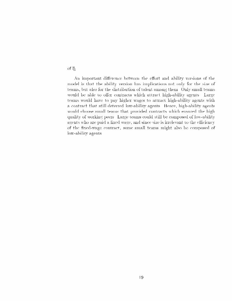
These two signi�cance levels are not necessarily equal. We can rewrite themusing the normality assumption and the de�nitions of A1 and A2. Equation(25) becomes

S(n; P ) = 1���Tn��n;H

�n

�= 1��

�Tn�nqh

�n

�= 1��

�Tn�ql�(n�1)qh�qh+ql

�n

�= 1��(A1 �

(qh�ql)

�n):

(27)

In the same way, equation (26) becomes

S(n+ 1; P ) = 1���Tn+1��n+1;H

�n+1

�= 1��

�Tn+1�(n+1)qh

�n+1

�= 1��(Tn+1�ql�nqh�qh+ql

�n+1)

= 1��(A2 �(qh�ql)�n+1

):

(28)

By equation (17), �n+1 > �n, so

(qh � ql)

�n>

(qh � ql)

�n+1: (29)

It follows from (29) and the fact that A1 = A2, that

�

A1 �

(qh � ql)

�n

!< �

A2 �

(qh � ql)

�n+1

!; (30)

so by equations (27) and (28) it is true that S(n; P ) > S(n+ 1; P ).Q.E.D.

34

REFERENCES.

Albanese, Robert and David Van Fleet. 1985. \Rational Behavior in Groups:The Free-Riding Tendency." 10 Academy of Management Review 244-255.

Baker, George, Michael Jensen, and Kevin J. Murphy. 1988. \Compensationand Incentives: Practice vs. Theory." 43 Journal of Finance 593-616.

Becker, Gary and George Stigler. 1974. \Law Enforcement, Malfeasance,and the Compensation of Enforcers." 3 Journal of Legal Studies 1-18.

Bendor, Jonathan and Dilip Mookherjee. 1987. \Institutional Structureand the Logic of Ongoing Collective Action." 81 American Political

Science Review 129-154.

Bickel, Peter and Kjell Doksum. 1977. Mathematical Statistics. San Fran-cisco: Holden-Day.

Bishop, John. 1987. \The Recognition and Reward of Employee Perfor-mance." 5 Journal of Labor Economics S36-S56.

Boyd, Robert and Peter Richerson. 1988. \The Evolution of Reciprocity inSizable Groups." 132 Journal of Theoretical Biology 337-356.

Brown, Charles and James Medo�. 1989. \The Employer-Size Wage E�ect."97 Journal of Political Economy 1027-1059.

Calvo, Guillermo, and Wellisz, Stanislaw. 1980. \Technology, Entrepreneurs,and Firm Size." 95 Quarterly Journal of Economics 663-678.

Coase, Ronald. 1937. \The Nature of the Firm. 4 Economica 386-405.

Coase, Ronald. 1988. \The Nature of the Firm: In uence." Journal of Law,

Economics, and Organization 33-47.

Doeringer, Peter, and Piore, Michael. 1971. Internal Labor Markets and

Manpower Analysis. Boston: D.S. Heath and Company.

35

Farrell, Joseph and Eric Lander. 1989. \Competition Between and WithinTeams: The Lifeboat Principle." Economics Letters, forthcoming.

Frank, Robert. 1985. Choosing the Right Pond. Oxford: Oxford UniversityPress.

Garen, John. 1985. \Worker Heterogeneity, Job Screening, and Firm Size."93 Journal of Political Economy 715-739.

Holmstrom, Bengt. 1982. \Moral Hazard in Teams." 13 Bell Journal of

Economics 324-340.

Holmstrom, Bengt. 1988. \Agency Costs and Innovation." Yale UniversityWorking Paper.

Kaldor, Nicholas. 1934. \The Equilibrium of the Firm." 44 Economic

Journal 60-76.

Kamien, Morton and Nancy Schwartz. 1982. Market Structure and Innova-

tion. Cambridge: Cambridge University Press.

Keren, M. and D. Levhari, 1983. \The Internal Organization of the Firm andthe Shape of Average Costs." 14 Bell Journal of Economics 474-488.

Klein, Benjamin and Keith Le�er. 1982. \The Role of Market Forces inAssuring Contractual Performance." 89 Journal of Political Economy615-641.

Latane, Bibb. 1984. \The Psychology of Social Impact." 36 American

Psychologist 343-356.

Lucas, Robert. 1978. \On the Size Distribution of Business Firms." 9 Bell

Journal of Economics 508-523.

Maddala. 1977. Econometrics. New York: McGraw Hill, 1977.

Marshall, Alfred. 1920. Principles of Economics. 8th edition. Reprinted,London: MacMillan Press, 1977.

McAfee, R. Preston and McMillan. 1989a. \Organizational Diseconomies ofScale." Mimeo, IRPS, University of California, San Diego, 10 April1989.

36

McAfee, R. Preston & John McMillan. 1989b. \Optimal Contracts forTeams." Mimeo, IRPS, University of California, San Diego, undated.

Medo�, J., and K. Abraham. 1980. \Experience, Performance, and Earn-ings." 95 Quarterly Journal of Economics 703-736.

Milgrom, P., and J. Roberts. 1988a. \An Economic Approach to In uenceActivities in Organizations." 94 Supplement American Journal of

Sociology S154-S179.

Milgrom, P., and J. Roberts. 1988b. \Bargaining Costs, In uence Costs,and the Organization of Economic Activity." Stanford UniversityDepartment of Economics Working Paper.

Mirrlees, James. 1974. \Notes on Welfare Economics, Information and Un-certainty." In Balch, McFadden, and Wu, eds., Essays on Economic

Behavior under Uncertainty. Amsterdam: North Holland.

Porter, Robert. 1983. \Optimal Cartel Trigger Price Strategies." 29 Journalof Economic Theory 313-338.

Rasmusen, Eric. 1989. Games and Information. Oxford: Basil Blackwell,1989.

Riley, John. 1979. \Informational Equilibrium." 47 Econometrica 331-359.

Scherer, Frederick, Alan Beckenstein, Erich Kaufer and R. Dennis Murphy.1975. The Economics of Multi-Plant Operation. Cambridge, Mass:Harvard University Press.

Schumpeter, Joseph. 1950. Capitalism, Socialism and Democracy. 3rd Edi-tion. New York: Harper and Row, 1975.

Shapiro, Carl and Joseph Stiglitz. 1984. \Equilibrium Unemployment as aWorker Discipline Device." 74 American Economic Review 433-444.

Shavell, Steven. 1985. \Criminal Law and the Optimal Use of NonmonetarySanctions as a Deterrence." 85 Columbia Law Review 1232-1263.

Sra�a, Piero. 1926. \The Laws of Returns Under Competitive Conditions."36 Economic Journal 535-50.

37

Stigler, George. 1958. \The Economies of Scale."1 Journal of Law and

Economics 54-71.

Stigler, George. 1962. \Information in the Labor Market." 70 (Supplement)Journal of Political Economy 94-105.

Stigler, George. 1964. \A Theory of Oligopoly." 72 Journal of Political

Economy 44-61.

Sugden, Robert. 1986. The Economics of Rights, Co-operation & Welfare,Oxford: Basil Blackwell, 1986.

Viner, Jacob. 1931. \Cost Curves and Supply Curves." 3 Zeitschrift fur

Nationalokonomie 23-46. Reprinted in Readings in Price Theory, ed.George Stigler and Kenneth Boulding. Homewood, Illinois: Irwin,1952.

Williamson, Oliver. 1967. \Hierarchical Control and Optimum Firm Size."75 Journal of Political Economy 123-138.

Williamson, Oliver. 1985. The Economic Institutions of Capitalism. NewYork: The Free Press, 1985.

Zenger, Todd. 1989. \Organizational Diseconomies of Scale: Pooling vs.Separating Labor Contracts in Silicon Valley." Ph.D. dissertation,University of California, Los Angeles.

38

Footnotes.

We would like to thank Steven Lippman, Ivan Png, Emmanuel Petrakis,Steven Postrel, Robert Topel, and Sang Tran for helpful comments. The datawas made available in part by the Inter-university Consortium for Politicaland Social Research.

1. See page 265 of Marshall (1920): \In other words, we say broadlythat while the part which nature plays in production shows a tendency todiminishing return, the part which man plays shows a tendency to increasingreturn. The law of increasing return may be worded thus:| An increase oflabour and capital leads generally to improved organization, which increasethe e�ciency of the work of labour and capital."

2. Schumpeter (1950), p. 101. More recent work along these lines includesLucas (1978) and Calvo and Wellisz (1980), who argue that high-ability man-agers will go to large �rms where their greater capacity to manage can be putto better use. This is a valid point, but our model will assume that the indi-vidual contribution of an agent to the team's output is the same regardlessof the team's size. We will try to isolate just one e�ect, and, like techno-logical economies of scale, the increasing sphere for talent could swamp thedisincentive e�ect we �nd for large teams.

3. See, e.g., Stigler's 1958 article on the Survivor Principle.

4. See Williamson (1985, Chapter 6) for a more complete discussion of theconstraints faced by large �rms in replicating small �rm incentives throughmultiple subunits.

5. Strictly speaking, the probability of avoiding a Type I error is the sizeof the test, and a test of size 0.95 is a test of signi�cance level 0.95, 0.94,0.93, and so forth. Since the term \size" is somewhat obscure (it is omittedfrom the index of many statistics texts), we will use \signi�cance level" here,with the understanding that we mean the test's highest signi�cance level.

6. One textbook that uses this test as an example in discussing thesestatistical points is Bickel & Docksum (1977). See Chapters 5 and 6, andespecially pages 168-71, 192, and 198.

39

7. The question of why costly punishments are used is also a lively ques-tion in the economics of crime. Shavell (1985) is a recent reference.

8. Our output distribution satis�es those assumptions, which means thatany size team can achieve \almost" the �rst-best if penalties are unbounded.

9. A third possibility is that both ability and e�ort vary between agents.We do not address that here; for a discussion, see McAfee and McMillan(1989b).

10. Some of these control variables may depend on whether it is e�cientfor the �rm to use incentive contracts. Since unions frown on incentive pay,for example, it might be that large �rms, for which a at wage might bemore e�cient, would resist unionization less strongly. If that is true, then bycontrolling for unionization we underestimate the e�ect of �rm size.

11. These values were determined by calculating the e�ect of tenure at 3years and then subtracting the e�ect of tenure at 2 years. For instance, thevalue 1.84% was calculated: 3(:0194) + 32(�:002)� 2(:0194) + 22(�:0002).

12. We have also performed the regressions for a subsample of CPS datacovering just professional and technical employees, whose output is partic-ularly hard to measure. The results are similar. Similar regressions werealso performed for a subsample that included only non-union males. Theseresults were also similar and, indeed, stronger than the results in Table 2.

13. F(120,120) = 1.35 at the 5 percent level, 1.53 at the 1 percent level(Maddala 1977, pp. 510-11). The lowest F-statistic in Table 2 is 1.494, andthe lowest sample size is 755, so every test is clearly signi�cant.

14. For surveys of this literature, see Albanese and Fleet (1985) andLatane (1981).

40

SCRAPS.

Lemma 1's statement that a larger sample produces a worse test is coun-terintuitive at �rst sight, because we are used to thinking about statisticaltests for the di�erence between the mean and a constant. For a �xed signif-icance level, such as 95 percent, the power of such a test increases with thesample size if the errors are independent, which seems to imply the oppositeof Lemma 1. But that is not the relevant test here. Rather, we are testingfor the presence of one shirking agent. The value in our alternative hypoth-esis is not a constant, but a variable that gets closer to the value in the nullhypothesis as the sample size increases. Speaking

loosely, Lemma 1 says that the increasing di�culty of distinguishing thealternative hypothesis outweighs the increasing precision of the estimate.

Another curious feature of Lemma 1 is that shirking in the larger team isharder to catch despite the fact that as the team size increases, the varianceof output per agent may decrease. If the disturbances are independent, thevariance of output per agent equals

v2n =�2

n; (31)

and if the errors are perfectly correlated it equals

v2n = �2: (32)

Hence, one might think that team size should not matter if the disturbancesare perfectly correlated, and that the larger team should be superior if thedisturbances are less than perfectly correlated. This is wrong. Output perteam member is not the relevant variable; its variance may fall to zero as nincreases, but that does not tell us that detecting a single deviator becomeseasier, since the individual disturbance's share of the total noise also falls asn increases.

|||||||||||||||||||||

41

From: tzengerDate: Mon, 4 Dec 89 15:56:33 pst Message-Id: <8912042356.AA25681To: facrasSubject : reviseddocument

Dear Eric,

This is the revised document. I made the change we talked about onpage 4, but I think it may need to be changed further in conjunction withthe revisions you make on page 19 regarding the Holmstrom article. I havemoved the proof to the Appendix and have dropped the counterintuitivenessdiscussion. I have also altered H1 and the su surrounding discussion.

Todd

Pfe�er, Je�rey and Langton, Nancy. 1988. \Wage Inequality and the Or-ganization of Work: The Case of Academic Departments." 33 AdministrativeScience Quarterly 588-606.

|||||||||||||||||||||

42