Discussion Papers in Economics

No. 2000/62

Dynamics of Output Growth, Consumption and Physical Capital in Two-Sector Models of Endogenous Growth

by

Farhad Nili

Department of Economics and Related Studies University of York

Heslington York, YO10 5DD

No. 1999/33

Stability and Equilibrium in Decision Rules: An Application to Duopoly

by

John Bone and Huw Dixon

Stability and equilibrium in decision rules: an

application to duopoly*

John Bone and Huw Dixon

Department of Economics and Related StudiesUniversity of YorkYork YO10 5DD

UK

jdb1@york.ac.uk ; hdd1@york.ac.uk

November 1999

Abstract

This paper analyses an indefinitely-repeated Cournot duopoly. Firms select simple dynamic

decision rules which, taken together, comprise a first-order linear difference equation system. A

boundedly-rational objective function is assumed, by which the firm’s payoff is its profit at the

point of convergence, if any. Stable Nash equilibria are characterised and located in output space,

stability in this context being equivalent to subgame-perfection. Comparable results are derived

for a conventional discounted-profit objective function, where this equivalence does not hold, but

where stability may nevertheless be of intrinsic interest. In either context, stability is incompatible

with joint profit maximisation.

* This paper is part of the project Evolution, oligopoly and competitiveness, funded by the ESRC,

grant number R000 23 6179. Comments are very welcome.

1 See, for example, Stanford (1986a), Klemperer and Meyer (1989), or Grossman (1981).

1

1 Introduction and overview

In this paper we analyse an indefinitely-repeated Cournot duopoly, within a framework motivated

by the idea of bounded rationality. Characteristic of this is the proposition that computational

simplicity is valuable to agents. In our model, simplicity is an issue at two levels. The first, and

more familiar, is that of the firm’s strategy. Among the simplest types of strategy, in this dynamic

context, is the Reaction Function, which gives the firm’s current output as a time-independent

function of its rival’s immediately previous output. Similarly, a Supply Function has as its only

argument the immediately previous market price. Strategies of this kind have received much

attention in the literature1, perhaps reflecting a widespread, if tacit, assumption that agents value

simplicity.

But the second level is that of the objective function, in terms of which firms identify their

(mutually) optimal strategies. Even if both firms’ strategies are very simple, the implied sequence

of outputs can be highly complicated and, therefore, difficult to evaluate. So firms might be

forced, or choose, to simplify this task. One possibility, which we explore in this paper, is that a

boundedly-rational firm evaluates an output sequence only at its point of convergence, if any. In

the case of a convergent sequence, this is effectively equivalent to a fully-rational firm with a zero

discount rate, using a limit-of-mean-profit criterion. But it is stronger than this criterion, in that

it places a zero value on non-convergent sequences.

Our analysis focuses on the asymptotic stability of outputs, in a Nash equilibrium. Given the

assumed objective function, stability here is equivalent to subgame-perfection. For a fairly simple

class of strategy, to be defined shortly, we show that almost any profitable output point can be

supported as a stable, boundedly-rational equilibrium. Notably excluded, however, is the duopoly

contract curve, comprising points of mutual profit maximisation.

We also analyse stability in the fully-rational, discounted profit case. As already noted, our

boundedly-rational equilibrium is largely equivalent to the limiting (zero discounting) case. But

in the fully-rational context stability does not imply subgame-perfection. Indeed, we find here that

2 It is well known that subgame-perfect equilibria can be sustained by discontinuous triggerstrategies, as in Friedman (1971) and Abreu (1986). However, Friedman and Samuelson (1994)showed that continuous versions of such strategies could be found.

2

linear Reaction Functions, for example, can support stable equilibria where subgame-perfection

is known to require rather more complex strategies. The lower the discount rate, the larger is the

set of output points thus supportable. This raises the possibility of stability constituting a weak

form of equilibrium refinement for fully-rational firms constrained to the simplest of strategies.

For the purposes of exposition, the paper deals first with the fully-rational case. Here, we are

interested in strategy pairs which satisfy three criteria:

Q Equilibrium, i.e., the mutual optimality of each firm’s strategy;

Q Stationarity of the generated output sequence, which means simply that outputs (and thus

the price) are constant from one period to the next;

Q Stability, i.e., re-convergence to the stationary point following any deviation from it.

Taking only the first two criteria, we might ask whether a given output vector can be supported

as a stationary equilibrium, i.e., as the stationary output sequence of a Nash equilibrium strategy

pair. It may easily be shown that, given concave profit functions, any profitable output point can

be thus supported (Proposition 1), and that this requires only (linear) Reaction Functions.

Subgame-perfection is, of course, more demanding. Thus, Stanford (1986a) demonstrates that

Reaction Functions (linear or otherwise) can support subgame-perfect equilibria only at the

standard Cournot equilibrium point. Friedman and Samuelson (1994) use the term single-period

recall function (SPRF) to describe a strategy which gives a firm’s output as a function of the

immediately previous outputs of both firms, and of which the Reaction Function (as defined here)

is a special case. They identify a class of continuous, non-linear, SPRFs capable of supporting a

subgame-perfect equilibrium at any profitable output point.2 This complements Stanford’s result,

and also that of Robson (1986), who shows that linear SPRFs can support such equilibria only

3

at the Cournot point. Such results are important because they tell us something about the degree

of strategic complexity required to support (subgame-perfect) equilibria. And complexity is of

interest, perhaps, because we can more plausibly imagine real firms using simple rules than

complex ones. As already suggested, this idea could be articulated in terms of bounded rationality,

by supposing that the use of a more complex rule is more demanding on a firm’s limited or costly

computational resources.

The assumption in this paper is that both firms adopt linear SPRFs which, as noted, are

insufficient for a subgame-perfect equilibrium other than at the Cournot point. However, our main

interest is not subgame-perfection as such, but rather the third criterion listed above, i.e., that of

stability. We find (Proposition 2) that linear SPRFs can support stable equilibria at a wide range

of output points. Notably excluded, however, are points of mutual profit-maximisation, i.e., the

contract curve. At best, in the limiting case of a zero discount rate, equilibria here may be “semi-

stable” in that there is re-convergence, following any deviation, but generally to some other point,

off the contract curve. We also consider two special cases of linear SPRF. The first is a Reaction

Function; here the stable equilibria comprise a cross-shaped set containing the two firms’ Cournot

(contemporaneous) best-response curves. The second is a Supply Function; here the stable

equilibria form a curved band running close to, but strictly above, the contract curve. In each case,

the size of the corresponding set is positively related to the per-period discount factor, i.e.,

negatively related to the discount or interest rate.

We then similarly analyse a boundedly-rational equilibrium. Just as in the fully-rational case,

stationary equilibria may be found at any profitable output point (Proposition 3). The significance

of stability, in this context, is that it is here equivalent to subgame-perfection (Propositions 4a and

4b). Stable equilibria, while more widespread than in the fully-rational case, are not quite

ubiquitous (Proposition 5). Again notably excluded are points on the contract curve. Equilibria

here are, at best, semi-stable. But they cannot be subgame-perfect.

The paper is structured as follows. In section 2 we define and elaborate our assumed class of

strategies. Section 3 outlines our assumptions concerning the firm’s profit function. Conventional,

fully-rational, stationary equilibria are characterised in section 4. The stability condition is

4

introduced in section 5, and applied to the fully-rational equilibrium (Proposition 2). Finally,

section 6 contains our analysis (Propositions 3-5) of boundedly-rational equilibria.

2 The Decision Rule

The model comprises two firms producing an homogeneous good. In each period ,(t'0,1,2,..)

each firm produces an output level , giving an output vector . We(i'1,2) xi,t xt' (x1,t ,x2, t)

assume no restriction on the output space other than that it is real, so that the set of feasible

output vectors is . Let denote an entire sequence of suchX/{xt * xt0ú2 } P' +x0 , x1 , x2 , . .,

output vectors. We describe as stationary (at ) any output sequence such that forx0X P xt'x

all t.

Governing each firm’s behaviour is a time-independent decision rule which makes a linearxi,t

function of the outputs of both firms in the immediately preceding period. This first-order linear

decision rule (FOLDR) is defined by a real triple such that:Di' (ai ,bi ,ci )

xi,t%1 ' aixi, t % bi xj,t % ci (i … j)

This is a special (i.e., linear) case of what Friedman and Samuelson (1994) call a single-period

recall function. Two subclasses of FOLDR which will be of interest are:

(i) A Reaction Function (RF), defined by , in which firm iNs output is a function onlyai'0

of firm jNs (immediate past) output.

(ii) A Supply Function (SF), defined by , in which firm iNs output is, in effect, a functionai'bi

only of the (immediate past) market-clearing price.

At the outset each firm adopts a strategy comprising an initial output and a(t'0) Fi' +xi,0 ,Di,

3 Notice that we use x with a single subscript to denote either the (timeless) output of agiven firm (i or j), or the output vector in a given time period (t). While convenient, this ispotentially ambiguous if the subscript is a numeral. Hereafter, single subscripts 1 or 2 refer onlyto the firms, while 0 refers to the initial time period.

5

FOLDR. The strategy pair generates a unique output sequence which we call itsF'(F1,F2) PF

trajectory. The trajectory of is stationary at only if, for each i :3F x'(x1,x2)

(1)xi ' ai xi % bixj % ci

Given , let denote the set of all satisfying (1). We call this the stationary set for .Di S i(Di) x0X Di

A stationary solution for is any:D'(D1,D2)

x 0 S(D) / S1(D1) _ S2(D2)

A strategy pair can be equivalently represented as . From the definition ofF' (F1,F2) F' +x0 ,D,

, it follows that the trajectory of is stationary if and only if .S(D) F' +x0 ,D, x00S(D)

We describe as regular any for which , in which case (1) may be rewritten as:Di ai…1

(2)xi ' $xj % (i

where:

and$i /bi

1&ai

(i /ci

1&ai

We similarly describe as regular any of which each is regular. For a regular ,D'(D1,D2) Di D

therefore, comprises solutions to (2) for each simultaneously. There will be exactlyS(D) i'1,2

one such solution, unless . In that case the two stationary sets will either coincide (if$1$2' 1

), giving infinitely many stationary solutions, or fail to intersect, giving none.(i' $i(j

6

3 Profit in a single period

We consider equilibria within , where:SdX%%dX

andX %%/{x0X * x1,x2$0} S / {x0X %% * B1(x),B2(x) >0}

For any , the profit for firm i in period t is given by:xt0X%%

Bi(xt) ' xi, t f (x1,t%x2,t) & gi( xi,t )

where is the market-clearing price and is firm i’s total cost. We assume thatf ( x1,t%x2,t) gi( xi,t )

each of these functions is differentiable, and that for all . We also assume that, withinf )<0 x0S

, is quasiconcave .X%% Bi(.)

Figure 1: A typical iso-profit contour

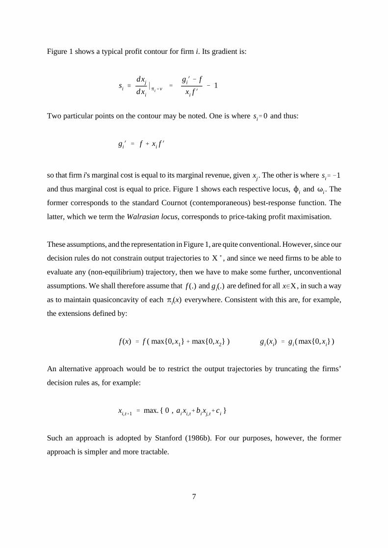
7

Figure 1 shows a typical profit contour for firm i. Its gradient is:

si /dxj

dxi

*Bi'v 'giN & f

xi f N& 1

Two particular points on the contour may be noted. One is where and thus:si'0

giN ' f % xi f N

so that firm i's marginal cost is equal to its marginal revenue, given . The other is where xj si'&1

and thus marginal cost is equal to price. Figure 1 shows each respective locus, and . TheNi Ti

former corresponds to the standard Cournot (contemporaneous) best-response function. The

latter, which we term the Walrasian locus, corresponds to price-taking profit maximisation.

These assumptions, and the representation in Figure 1, are quite conventional. However, since our

decision rules do not constrain output trajectories to , and since we need firms to be able toX %%

evaluate any (non-equilibrium) trajectory, then we have to make some further, unconventional

assumptions. We shall therefore assume that and are defined for all , in such a wayf (.) gi(.) x0X

as to maintain quasiconcavity of each everywhere. Consistent with this are, for example,Bi(x)

the extensions defined by:

f (x) ' f ( max{0,x1}% max{0,x2} ) gi(xi) ' gi( max{0,xi})

An alternative approach would be to restrict the output trajectories by truncating the firms’

decision rules as, for example:

xi,t%1 ' max. { 0 , ai xi,t%bixj, t%ci }

Such an approach is adopted by Stanford (1986b). For our purposes, however, the former

approach is simpler and more tractable.

8

4 Stationary, fully-rational equilibria

In a fully-rational equilibrium, each firm’s strategy maximises the discounted sequence of that

firm’s profits, given the strategy of its rival. For firm j this is:

Aj(P) / j4

t'0*tBj(xt)

The discount factor we assume to be common to the two firms; this simplifies the*0(0,1)

analysis, but is not crucial to it. Consider some strategy pair such that is stationaryF'(F1,F2) PF

at . Thus for each firm i:x

and (3)xi,0 ' xi xi ' ai xi % bi xj % ci

Given , under what conditions is optimal for firm j?Fi Fj

Suppose firstly that . Since is stationary, it follows that and ,bi'0 PF xi,0' xi Di' (ai , 0 , (1&ai) xi)

i.e., that firm i’s output is independently stationary at . But then is optimal if and only if xi Fj x

maximises each subject to . A necessary condition for this is , i.e., that theBj(xt) xi,t' xi sj(x)'0

slope of firm j’s iso-profit contour be zero. This is also sufficient, given quasiconcavity of .Bj(.)

We can thus verify the existence of a repeated Cournot equilibrium, where each firm’s output is

independently stationary at defined by .x0S s1(x)'s2(x)'0

Now suppose instead that . Given that satisfies (3), is optimal if and only if bi…0 Fi Fj PF

maximises subject to, for all t:Aj(P)

andxi,0 ' xi,0 xi,t%1 ' ai xi,t % bixj, t % ci

Given these constraints, and given that is stationary at , then for any T:PF x

(4)MAj

Mxj,T

' & *TMBj(x)

Mxi

sj(x) & *bij4

t'T

(*ai)t&T

4 Note the formal similarity between this proposition and the ubiquity of consistent-conjectures equilibria, as demonstrated by Klemperer and Meyer (1988), and similarly central towhich is the tangency of the (conjectured) reaction function of one firm to an iso-profit contourof the other.

9

For to be optimal it is necessary that (4) is zero for every T. That is:Fj

and (5)&1< *ai <1 sj(x) '*bi

1&*ai

Note that (5) also characterises the optimal given and , and therefore someFj &1< *ai <1 bi'0

of the Cournot equilibrium strategies.

For an illustrative interpretation of (5), suppose that is an RF, so that and the first partDi ai'0

of the condition is satisfied. Then any single-period output perturbation by firm j induces an

output response by firm i in, and only in, the following period. The ratio of the latter to the former

is , here the gradient of . The second part of (5) then requires that the net (discounted)bi S i(Di)

effect on firm j’s profit is zero. In the limiting case with zero discounting , this implies that(*'1)

firm j’s iso-profit contour is tangent to . S i(Di)

For FOLDRs in general, (5) is most easily interpreted in this limiting case, where the first part of

the condition is that . This implies that following any single-period perturbation in firmai0(&1,1)

j’s output, firm i’s output will re-converge to . If this were not the case, then firm j couldxi

thereby induce, for example, an indefinite (unlimited) reduction in firm i’s output. Given that

, the cumulative total of all subsequent output responses by firm i converges to , asai0(&1,1) $i

a proportion of firm j’s initial perturbation. For marginal perturbations, the second part of (5)

requires that the net (in this case, undiscounted) effect on firm j’s profit is zero. Again, in this

limiting case this implies that firm j’s iso-profit contour is tangent to . S i(Di)

In addition to being necessary, (5) is also sufficient for optimality if is concave, whichAj(P)

would follow from concavity of . It would also be sufficient were only quasiconcave,Bj(.) Aj(P)

but this does not follow from quasiconcavity of . Given a sufficiently strong assumption ofBj(.)

this kind, stationary equilibria are ubiquitous in S, as stated in the following Proposition.4

10

Proposition 1 Given concavity of , then for any and any there existsBi(.) x0S *0(0,1)

an equilibrium such that is stationary at x.F'+x0,D, PF

Proof: Given x and *, put , and construct D to satisfy (1) and (5), i.e,:x0'x

*ai0 (&1,1) bi' (1&*ai)sj(x)

*ci ' (1&ai)xi& bi xj

QED

Note that among the satisfying (1) and (5) there is always an RF-pair, for which:D

(6)bi'sj(x)

*

Thus, stationary RF equilibria are ubiquitous. This is not true, however, of SF equilibria. From

the second condition in (5), an equilibrium in SFs requires that, for each firm i:

(7)ai ' bi'sj(x)

* (1% sj(x))

But then the first condition in (5) can then be satisfied only if for each firm. Thissi(x) >&½

restriction will be illustrated in the next section, where we derive the conditions under which such

equilibria are also asymptotically stable.

To conclude this section, however, we should comment on one aspect of our equilibrium analysis.

In deriving (5), we considered the effect on firm j’s (discounted) profits of a perturbation in xj,T

for any single T. Thus, (5) is necessary for a broad equilibrium in which is optimal, for firm j,Fj

among all possible trajectories consistent with . However, if firm j is restricted to strategies ofFi

the form then it cannot independently vary any single . We might therefore wishFj' +xj,0 ,Dj, xj,T

to consider a correspondingly narrow equilibrium, in which is optimal only among all . ButFj Fj

it is easily seen that (5) is necessary also for to be a narrow equilibrium. Consider(F1,F2)

alternative strategies comprising and each of which, in effect, fixesFj xj,0'xj Dj' ( aj ,0 , (1&aj) xj)

firm j’s output at . Among these strategies:xj,t'xj

11

(8)dAj

dxj

' j4

t'T

MAj

Mxj,T

Given , the selection of such a strategy with gives the same stationary trajectory, and theFi xj' xj

same payoff to firm j, as does the selection of . So for to be optimal among it is necessaryFj Fj Fj

for (8) to be zero, when evaluated at . Given (4), this requires (5) as before.x

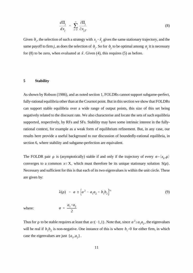
5 Stability

As shown by Robson (1986), and as noted section 1, FOLDRs cannot support subgame-perfect,

fully-rational equilibria other than at the Cournot point. But in this section we show that FOLDRs

can support stable equilibria over a wide range of output points, this size of this set being

negatively related to the discount rate. We also characterise and locate the sets of such equilibria

supported, respectively, by RFs and SFs. Stability may have some intrinsic interest in the fully-

rational context, for example as a weak form of equilibrium refinement. But, in any case, our

results here provide a useful background to our discussion of boundedly-rational equilibria, in

section 6, where stability and subgame-perfection are equivalent.

The FOLDR pair is (asymptotically) stable if and only if the trajectory of every D F' +x0 ,D,

converges to a common , which must therefore be its unique stationary solution .x0X S(D)

Necessary and sufficient for this is that each of its two eigenvalues is within the unit circle. These

are given by:

(9)8(D) ' a ± a 2 & a1a2 % b1b2½

where: a /a1%a2

2

Thus for to be stable requires at least that . Note that, since , the eigenvaluesD a0(&1,1) a 2$a1a2

will be real if is non-negative. One instance of this is where for either firm, in whichb1b2 bi'0

case the eigenvalues are just .{a1,a2}

12

In section 2 we noted the possibility of a regular D with infinitely many stationary solutions, where

the two firms’ (linear) stationary sets coincide, so that . Here, from (9):$1$2'1

8(D) ' 1 and 2a&1

The first eigenvalue applies to each of the stationary solutions. The other eigenvalue8(D)'1

applies to any other trajectory, all of which are linear and mutually parallel. If8(D)'2a&1

then they all converge, but not to the same stationary solution. We will describe such aa0(0,1)

D as semi-stable. It will be of significance in what follows.

We now characterise and locate sets of stable, stationary equilibria. Consider firstly a pair of RFs

which, from (9), is stable if and only if:

&1 < b1b2 < 1

From (6), a stationary equilibrium in RFs is therefore stable if and only if:

where . (10)&*2 < s(x) < *2 s(x)/ s1(x)s2(x)

Figure 2 sketches this in the special case of a linear demand function and identicalp' 1&x1&x2

quadratic costs . It shows the set , bounded above by the (linear) zero-profit contoursg(xi)'x 2i S

which intersect at the output vector , here denoted z. The output vector corresponding(1/3,1/3)

to the Walrasian (price-taking) equilibrium is , denoted w. The Cournot equilibrium is(1/4,1/4)

at , denoted c, and joint profit maximisation is achieved at , denoted m. The(1/5,1/5) (1/6,1/6)

curve passing through m is the contract curve, comprising points of mutual profit maximisation.

It is characterised by the mutual tangency of the two firms’ iso-profit contours, and thus by

. This is true also of the curve passing through w, but which comprises points of mutuals(x)'1

(local) profit minimisation. We call this the anti-contract curve. The figure also shows, for each

firm, the loci identified in section 3, which in this special case are linear. The Walrasian loci, ,Ti

are the lines intersecting at w. The Cournot loci, , are the lines intersecting at c. TheseNi

13

subdivide S into four main areas: two off-diagonal areas in which , and two on-diagonals(x)<0

areas in which . (This refers to the positive diagonal, connecting z to the origin.)s(x)>0

c

w

m

z

1/2

1/3

1/4

1/4 1/3 1/20

s(x)>1

s(x)>1

s(x)< !1

s(x)< !1

x1

x2

Figure 2: Stationary equilibria with stable RFs

The set of stationary equilibria in stable RFs, i.e., output points satisfying (10), is a strict subset

of S. At its largest, as , it approaches the shaded region in Figure 2. It always lies strictly*61

above the contract curve and below the anti-contract curve, along each of which . Off thes(x)'1

diagonal, it is bounded by curves along which . At its smallest, as , it reduces to thes(x)'&1 *60

cross formed by , which includes the Cournot point c. Each is characterised by ,N1^N2 Ni si(x)'0

and so satisfies (10) for any positive *.

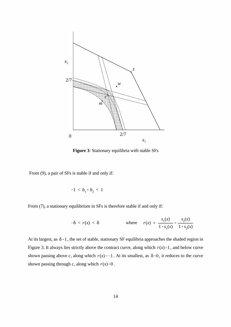
Figure 3 sketches the corresponding region for Supply Functions. Recall from the previous section

that SFs, unlike RFs, can support stationary equilibria only where for each firm. Thesi(x) >&½

relevant (linear) boundaries, below which this is satisfied, are shown intersecting above c.

14

x1

x2

2/7

z

w

cm

2/7

0

Figure 3: Stationary equilibria with stable SFs

From (9), a pair of SFs is stable if and only if:

&1 < b1% b2 < 1

From (7), a stationary equilibrium in SFs is therefore stable if and only if:

where &* < r(x) < * r(x) /s1(x)

1%s1(x)%

s2(x)

1% s2(x)

At its largest, as , the set of stable, stationary SF equilibria approaches the shaded region in*61

Figure 3. It always lies strictly above the contract curve, along which , and below curver(x)'1

shown passing above c, along which . At its smallest, as , it reduces to the curver(x)'&1 *60

shown passing through c, along which .r(x)'0

15

Having looked in particular at RFs and SFs, we now consider FOLDRs in general. For any

satisfying the equilibrium condition (5), the eigenvalues may be written as:D' (D1,D2)

(11)8(D) ' a ± a 2 & a1a2 %s(x)

*2(1&*a1)(1&*a2)

½

where . We have found that output points on the contract curve cannot be supported*ai0(&1,1)

as stationary equilibria either in stable RF pairs or in stable SF pairs. It is readily established that

such points cannot be supported by stable FOLDRs at all. Suppose that , as on the contracts(x)'1

curve. From (11) it follows that:

8(D) '1*

and 2a& 1*

whereby at least one eigenvalue is not within the unit circle. Although at any point on the(1/*)

contract curve there exist stationary equilibria in FOLDRs, none of these is stable. In the limiting

case there exist stationary equilibria, with , which are semi-stable. Here, any(*'1) a0(0,1)

deviation from the stationary output trajectory will be followed by re-convergence, but in general

to some other stationary solution, off the contract curve.

So is a requirement for stability of stationary equilibria, notably excluding the contracts(x)…1

curve. The following is more specific.

Proposition 2 For there to exist an equilibrium such that D is stable and isF' +x0 ,D, PF

stationary at , it is necessary and (if each is concave) sufficientx0S Bj(.)

that .s(x)< *2

Proof: We first demonstrate necessity. Assume an equilibrium such that isF' +x0 ,D, PF

stationary at x. Suppose that . Then from (11) the eigenvalues are real, in whichs(x)>0

case D is stable only if:

*a* % a 2 & a1a2 %s(x)

*2(1&*a1)(1&*a2)

½

< 1

5 This can be confirmed by considering the arithmetic difference between the (positive)denominator and the numerator, and verifying that this must be non-negative. For any given a,this difference is minimised by setting , given which it is:a1'a2'a

2(*a*&*a) & (1&*2)a 2

This expression is a quadratic in each of its restrictions to, respectively, non-negative and non-positive values of a. As such, it is straightforward to verify that it is non-negative for any

.a0(&1,1)

16

which can be re-arranged to:

s(x)

*2<

1% a1a2& 2*a*

(1&*a1)(1&*a2)

Stability implies that , and therefore that the right-hand side cannot exceeda0(&1,1)

unity.5 So stability here requires that .s(x)<*2

We now demonstrate sufficiency. Given and such that , put *0(0,1) x0S s(x)<*2 x0'x

and construct a stable D satisfying (1) and (5). As in the proof of Proposition 1, put:

bi' (1&*ai)sj(x)

*ci ' (1&ai)xi& bi xj

Put also so that, from (11), D is stable if:a'0

&*2 < *2a 2i % (1& *2a 2

i ) s(x) < *2

This may be viewed as is a generalisation of (10), and interpreted as requiring the

average of 1 and to lie within the open interval . It is(*2a 2i )&weighted s(x) (&*2,*2 )

straightforward to verify (e.g., graphically) that, given any and , there*0(0,1) s(x)<*2

always exist to satisfy this.*ai0(&1,1)

QED

So is a necessary and (given concavity) sufficient condition for the existence of a stable,s(x)< *2

17

stationary equilibrium at x. The set of output points satisfying this can be visualised in Figure 2.

It comprises the set of stable RF equilibria, plus the two off-diagonal areas in which . Ats(x)#0

its smallest, as , it reduces to just these two areas (which together include the Cournot loci).*60

Elsewhere in S, i.e., where , it has the same boundaries as the set of stable equilibria ins(x)>0

RFs. At its largest, as , these are the contract curve and the anti-contract curve.*61

6 Subgame-perfection and a boundedly-rational equilibrium

In this section we analyse a boundedly-rational equilibrium, where stability and subgame-

perfection are equivalent. An equilibrium is subgame-perfect if the mutually–optimal strategies

would remain so, following any deviation in either firm’s output in any period. Stability also

concerns the consequences of output deviation, but not in any directly normative sense and, in the

fully-rational context, we have seen that the two criteria are not generally co-extensive. However,

they may be more closely related in the limiting case of zero discounting . Consider an(*'1)

equilibrium trajectory where the criterion of optimality, for each firm, is its ‘long-run’ profit. If

D is stable, then following any deviation output re-converges to the same long-run, mutually-

optimal point. A formal proposition of this kind is demonstrated by Stanford (1986b): with zero-

discounting, a stable equilibrium in RFs must be subgame perfect. We now define a FOLDR

equilibrium in which stability is not only sufficient, but also necessary, for subgame-perfection.

Assume that each firm j seeks to maximise:

if converges to some Bj(x) P x0X Uj(P) / 9 0 otherwise

The first part of this definition is equivalent to a limit-of-mean-profit objective function. This

criterion is commonly used, for example by Stanford, to represent zero discounting. Any output

sequence with bounded profits is evaluated as the limit of its mean per-period profit. In the case

of a convergent sequence, this is just the value to which each period’s profit converges.

6 This is similar in spirit to an assumption made by Klemperer and Meyer (1989, p.1247),i.e., that firms’ payoffs are zero when no unique equilibrium exists for given supply functions.

18

Although our approach has been to allow unbounded output sequences, it is consistent with this

for profit to be bounded, which is all that the limit-of-mean-profit criterion requires. So we could

follow Stanford in applying this criterion. However, even when suitably bounded, the computation

and evaluation of a non-convergent trajectory can be very difficult. A firm might therefore

economise on computational time and expense by simply attaching a zero value to non-convergent

output trajectories, as in the second part of the above definition.6 The first part of the definition

could similarly reflect computational constraints, rather than zero-discounting as such, for

convergent, but non-stationary, trajectories. So our objective function as a whole could be taken

to represent a form of bounded-rationality on the part of the firm.

Given this objective function, the characterisation of a stationary equilibrium at x is identical to

that of a convergent equilibrium, i.e., an equilibrium with a trajectory converging to x. In this

context, the former is just a special case of the latter. So we can more generally locate output

points at which there are convergent equilibria, among which there will always be a stationary

equilibrium. Furthermore, for an equilibrium with a stable D the initial output vector isx0

irrelevant. A stable equilibrium can be unambiguously located in output space by the unique

stationary solution , in the knowledge that this locates a convergent equilibrium for any .S(D) x0

Indeed, this is why such an equilibrium is subgame-perfect. These observations will be elaborated

more formally below. Firstly, though, we characterise a boundedly-rational equilibrium, by

considering some such that converges to . Given , under what conditions is F'(F1,F2) PF x Fi Fj

optimal for firm j?

Suppose firstly that , so that firm i’s output converges to , irrespective of firm j’s strategy.bi'0 xi

Thus any output trajectory which firm j can induce through its own strategy choice will converge,

if at all, only to some such that . But firm j can induce a trajectory converging to anyx0X xi' xi

such x, simply by choosing an appropriate convergent trajectory for its own output, i.e.:

aj0(&1,1) bj'0 cj ' (1&aj) xj

19

It follows that is optimal, in terms of the boundedly-rational objective function, if and only if Fj x

maximises subject to . Necessary and (given quasiconcavity) sufficient for this is thatBj(x) xi' xi

. The reasoning here closely parallels that in section 4, and it is straightforward to verifysj(x )'0

the existence of a stationary Cournot equilibrium, strategically identical to that in the fully-rational

case. In this boundedly-rational case we may also verify the existence of equilibrium trajectories

converging to, but not necessarily stationary at, the Cournot point.

Now suppose instead that . Any trajectory which firm j can induce through its own strategybi…0

choice will converge, if at all, only to some . But firm j can induce a trajectoryx0S i(Di)

converging to any such x, as confirmed in the following Lemma:

Lemma 1 For any such that , and for any , there exists some such thatDi bi…0 x0S i(Di) Dj

is stable and .D'(D1,D2) S(D)'{x}

Proof: Given and x, construct a stable D satisfying (1), e.g.:Di

aj'&ai bj'&a 2j /bi cj ' (1&aj) xj& bjxi

QED

Note that is crucial to this proposition. If instead , as in a Cournot equilibrium, thenbi…0 bi'0

the eigenvalues are , so that firm j cannot independently ensure stability.{a1,a2}

So, given that , firm j can induce a trajectory converging to, and only to, any . Itbi…0 x0S i(Di)

follows that is optimal, in terms of the boundedly-rational objective function, if and only if Fj x

solves:

max. subject to: Bj(x) xi ' ai xi % bixj % ci

Necessary and (given our assumption of quasiconcavity) sufficient for this is that:

and (12)ai…1 sj(x) 'bi

1&ai

/ $i

20

which may be compared with (5), the corresponding condition for fully-rational equilibrium. The

second part of (12) confirms the equivalence to the limiting case of zero discounting .(*'1)

However the first part, that be regular, is considerably weaker than the limiting case of theDi

corresponding part of (5), which is that . This reflects our strong assumption that theai0(&1,1)

boundedly-rational firm places a zero value on any non-convergent trajectory.

Note that (12) also characterises any (convergent) Cournot equilibrium in which is regular, andDi

therefore where is optimal if and only if maximises subject to . A CournotFj x Bj(x) x0S i(Di)

equilibrium in which cannot be thus characterised, since here . Di'(1,0,0) S i(Di)'X

From (12) we can confirm that stationary, boundedly-rational equilibria are ubiquitous.

Proposition 3 For any there exists a boundedly-rational equilibrium suchx0S F' +x0 ,D,

that is stationary at x.PF

Proof: Given x, put , and construct D to satisfy (1) and (12), i.e.:x0'x

ai…1 bi' (1&ai) sj(x) ci ' (1&ai)xi& bi xj

QED

Among the equilibria characterised by (12) are those which are (perhaps) non-stationary, but in

which is stable, with a unique stationary solution at . Such cases are really equilibria inD x

decision rules rather than in strategies as such. Furthermore, they are subgame-(D1,D2) (F1,F2)

perfect. An equilibrium is subgame-perfect if and only if at any future time t, theF' (F1,F2)

adopted strategies remain mutually optimal from any feasible position, whether or not on the

equilibrium trajectory. In the present context, this requires that at any time t, is optimal givenDj

, and given any feasible . But all features of the market are time-independent, including theDi xt

objective functions. So this is equivalent simply to requiring that are mutually optimal,(D1,D2)

regardless of .x0

21

Proposition 4a If is a boundedly-rational equilibrium, and if is stable, thenF' +x0,D, D

any is a subgame-perfect boundedly-rational equilibrium.F' +x0 ,D,

Proof: If is stable then the trajectory of any converges to which by assumption,D F' +x0,D, x

for each firm j, maximises subject to . (Note that this applies also to theBj(x) x0S i(Di)

Cournot equilibrium, where stability entails that is regular.) Given , therefore, firmD Di

j can induce no better trajectory than this. So is a boundedly-rationalF' +x0,D,

equilibrium. Since the same argument applies at any subsequent time t, for any given ,xt

the equilibrium is also subgame-perfect.

QED

This is similar to the proposition demonstrated for RFs under zero-discounting by Stanford

(1986b). Given our boundedly-rational objective function, however, the following converse

proposition is also true.

Proposition 4b A boundedly-rational equilibrium , with a trajectory convergingF' +x0,D,

to , is subgame-perfect only if is stable.x D

Proof: Assume that is not stable. We require to show that the equilibrium is thereforeD'(D1,D2)

not subgame-perfect.

Suppose firstly that for some firm i. If is not stable then there is somebi…0 D'(D1,D2)

such that the trajectory of does not converge to . But from Lemma 1x0…x0 F' +x0,D, x

there exists some , with , such that the trajectory of does converge toD Di'Di F' +x0,D,

. So, given , is not the best response to . Thus, the equilibrium is not subgame-x x0 Dj Di

perfect.

Suppose instead that for each firm i, and therefore that the eigenvalues are .bi'0 {a1, a2}

If is not stable, then for at least one firm j. Lemma 1 does not apply here,D ajó(&1,1)

since the other eigenvalue is . However, irrespective of the value of , there is some ai ai x0

such that the trajectory of does not converge to , but would do so wereF' +x0,D, x

22

. Any such that is of this type, these being the eigenvectorsaj0(&1,1) x0…x xi,0' xi

corresponding to the eigenvalue . So for at least one firm j there exists some , givenaj x0

which is not the best response to . Thus, the equilibrium is not subgame-perfect. Dj Di

QED

So a boundedly-rational equilibrium is subgame-perfect, and thus essentially anF' +x0,D,

equilibrium in decision rules, if and only if is stable. It now remains to locate the set of suchD

equilibria. We know, from Proposition 3, that a stationary equilibrium can be found at any

profitable output point. But this is not so for stable equilibria. There are boundedly-rational

equilibria with stationary (and otherwise convergent) trajectories for which cannot be stable.D

Significantly, these occur on the contract curve. Consider an equilibrium , with aF' +x0,D,

trajectory converging to some on the contract curve, i.e., such that . From (12) itx s(x)'1

follows that , i.e., that the two firms’ stationary sets coincide. So there are infinitely many$1$2'1

stationary solutions other than , and is not stable. At best, i.e., if , is semi-stable.x D a0(0,1) D

But this does not suffice for subgame-perfection. There exists some (arbitrarily close to )x0 x0

such that the trajectory of converges to some stationary solution other than , and less+x0,D, x

profitable for at least one firm j. But from Lemma 1 we know that, given , there is some Di Dj…Dj

which does ensure convergence to . So, given such an , are not mutually optimal.x x0 (D1,D2)

Just as in the fully-rational case, therefore, is necessary for a stable, boundedly-rationals(x)…1

equilibrium to be located at x. In this case, we may show that it is also sufficient.

Proposition 5 For there to exist a boundedly-rational equilibrium such that DF' +x0 ,D,

is stable and converges to , it is necessary and sufficient thatPF x0S

.s(x)… 1

Proof: Necessity has already been demonstrated. To demonstrate sufficiency, construct a stable

D which, given x , satisfies (1) and (12). As for Proposition 3, put:

bi' (1&ai) sj(x) ci ' (1&ai)xi& bi xj

23

Put also , so that from (11) D is stable if:a'0

&1 < a 2i % (1& a 2

i ) s(x) < 1

Given that , it is always possible to find some which satisfies this.s(x)…1 ai…1

QED

So there is a stable boundedly-rational equilibrium located (i.e., with its stationary solution) at any

profitable output point except on the contract curve and the anti-contact curve. This near-ubiquity

reflects our strong assumption that non-convergent trajectories have zero value, and therefore that

each firm’s FOLDR need only be regular. By contrast, in the limiting case of the stationary(*'1)

fully-rational equilibrium the corresponding existence condition is , which additionallys(x)<1

excludes output points below the contract curve and above the anti-contract curve.

The sets of stable RF and SF boundedly-rational equilibria can similarly be deduced from the

limiting cases of their respective stationary, fully-rational counterparts. For RFs this is

straightforward; in Figure 2 the relevant set is represented by the shaded region. For SFs note that

the second condition in (12) requires that, for each firm i:

ai ' bi'sj(x)

1%sj(x)

Given which the first condition in (12) is automatically satisfied. So, in the boundedly-rational

case, the (linear) boundaries shown in Figure 3 do not apply. The set of stable SF equilibria is just

the curved region bounded below by the contract curve.

To summarise: we have established that stable, boundedly-rational equilibria in FOLDRs can be

found almost anywhere in (positive-profit) output space. Excluded, however, are points of mutual

profit-maximisation on the contract curve. There are boundedly-rational equilibria with outputs

stationary at such points, but these are not stable and, therefore, not subgame-perfect.

24

References

Abreu D, (1986); “Extremal equilibria of oligopolistic supergames”, Journal of Economic

Theory 39:191-225

Friedman J, (1971); “A noncooperative equilibrium for supergames”, Review of Economic

Studies 38:1-12

Friedman J, and L Samuelson, (1994); “Continuous reaction functions in duopolies”, Games

and Economic Behavior 6:55-82

Grossman S, (1981); “Nash equilibrium in the industrial organization of markets with large

fixed costs”, Econometrica 49:1149-77

Kelmperer P, and M Meyer, (1988); “Consistent conjectures equilibria”, Economics Letters

27:111-15

Kelmperer P, and M Meyer, (1989); “Supply function equilibria in oligopoly under

uncertainty”, Econometrica 57:1243-77

Robson A, (1986); “The existence of Nash equilibria in reaction functions for dynamic models

of oligopoly”, International Economic Review 27:539-44

Stanford W, (1986a); “Subgame perfect reaction function equilibria in discounted duopoly

supergames are trivial”, Journal of Economic Theory 39:226-232

Stanford W, (1986b); “On continuous reaction function equilibria in duopoly supergames with

mean payoffs”, Journal of Economic Theory 39:233-250