DISCUSSION PAPER

MTI Global Practice

No. 1 May 2018 Fritz F. Bachmair Jane Bogoev

ii

This series is produced by the Macroeconomics, Trade, and Investment (MTI) Global Practice of the World

Bank. The papers in this series aim to provide a vehicle for publishing preliminary results on MTI topics to

encourage discussion and debate. The findings, interpretations, and conclusions expressed in this paper

are entirely those of the author(s) and should not be attributed in any manner to the World Bank, to its

affiliated organizations, or to members of its Board of Executive Directors or the countries they represent.

Citation and the use of material presented in this series should take into account this provisional character.

For information regarding the MTI Discussion Paper Series, please contact the Editor, Ivailo Izvorski, at

iizvorski@worldbank.org.

© 2018 The International Bank for Reconstruction and Development / The World Bank

1818 H Street, NW Washington, DC 20433

All rights reserved

1

MTI DISCUSSION PAPER NO. 1

Abstract

The aim of this analysis is to quantify the losses from potential materialization of contingent

liabilities by applying a new methodology for the case of South Africa and, to assess their impact

on debt dynamics. Accordingly, we bring a novelty to this research by utilizing probabilities of

distress, which is a different approach compared to the existing, already applied methodology. The

central finding of the simulations conducted is that estimated losses from contingent liabilities, are

significantly lower in the first year when they materialize compared to the existing applied

methodology, and will gradually add up over time. Accordingly, the solvency and liquidity

situation in the country will deteriorate. For example, the largest deterioration will occur in the

debt to GDP ratio where the debt accumulation may be higher by 2.1 percent of GDP within three

years, compared to the baseline projection. What is more concerning is that the debt trajectory is

not stabilizing and losses incurred from materialization of contingent liabilities may become

significant driving factor of debt accumulation in medium-term. Ultimately, the current estimates

suggest that contingent liabilities may constitute a drag to fiscal policy in medium-term and their

long-term accumulation may jeopardize the debt sustainability of the country. In that respect, this

analysis suggests remedial measures and building protective buffers by the South African Treasury

in the case CLs materialize.

Corresponding authors: jbogoev@worldbank.org;

JEL Classification: E62, H60, H63, H68

Keywords: Contingent Liabilities, Debt, Debt Management, Public Finances, National Debt Forecast

2

Assessment of Contingent Liabilities and Their Impact on Debt Dynamics in

South Africa1

Fritz F. Bachmair, Jane Bogoev

1. Introduction

Sound public finances are critical to enable fiscal policy that promotes economic growth and

stabilizes economic activity through the business cycles. Sovereign balance sheets are exposed to

significant fiscal risks and may impair governments’ ability to exercise good fiscal policy.

Contingent liabilities (CLs) are an important type of fiscal risk. The materialization of CLs can

have significant impact on government finances, crowd out important spending during economic

downturns, or jeopardize fiscal and debt sustainability (International Monetary Fund, 2016).

In South Africa, specifically, CLs may constitute a major risk to government finances. Sluggish

economic performance in recent years has contributed to a deterioration of the fiscal balance and

a corresponding increase in government debt relative to GDP. At the same time, the profitability

of the state-owned corporations (SOCs) has declined. South African government has increasingly

supported SOCs not only through issuance of guarantees, but also through loans, subsidies, and

equity injections. To manage and mitigate the risks, the National Treasury of South Africa (NTSA)

has started implementing reform initiatives to manage such risks, including the assessment of

credit risk from exposure to SOCs, the publication of a fiscal risk statement, and SOCs governance

reform.

This analysis aims to contribute to the understanding of the potential impact from materialization

of CLs on government finances and debt dynamics in South Africa by applying a new

methodology. In particular, this includes analysis of the development of the solvency and liquidity

indicators such as, the path of public debt relative to GDP and debt service costs relative to

government revenues. While South Africa is exposed to CLs from large number of entities, we

focus on: I) The liabilities of the nine largest SOCs2 according to their asset size; II) Government

guaranteed power purchase agreements (PPAs) between Eskom; III) The state-owned electric

utility and independent power producers (IPPs); IV) Guarantees to public-private partnerships

(PPPs), and V) The Road Accident Fund (RAF).

1 Some of the data used in this analysis is obtained from the National Treasury of South Africa (NTSA) for which the authors are highly indebted. In particular, the methodology applied has crucially benefitted from the probabilities of distress calculated by NTSA, and without these, the new methodology applied might not be generally applicable. The World Bank Treasury has supported NTSA in recent years in reviewing and improving its analytical processes for credit risk management. The authors are also indebted to Mathew Verghis, Sebastien Dessus and Marek Hanusch for their comments and suggestions that significantly contributed for improvement of the quality of this paper. The views and opinions reflected in this note do not necessarily reflect that of the Executive Directors of the World Bank Board, or of the countries they represent. 2 SOCs included, in alphabetical order, are: Denel, the Development Bank of South Africa, Eskom, Landbank, the South African Post Office, the South African National Roads Agency, Telkom South Africa, Transnet, and South African Airlines. These SOCs account for 93 percent of the government’s guarantee portfolio.

3

We also considered including subnational (SN) debt in the analysis. However, the debt from 80

districts, local and provincial governments for which we were able to obtain data; amounts to only

0.92 percent of GDP. Hence, we rejected including SN debt. The types of CLs we focus on, have

been cited by many observers as the most critical.3 Accordingly, the focus of the NTSA in risk

management efforts4 and data availability, has narrowed our scope of assessment of CLs.

This paper is structured as follows: Section 2 outlines the methodology and data we employ, and

assumptions we make. Section 3 discusses the results. The concluding remarks and policy

recommendations for risk management are presented in Section 4.

2. Data and methodology

To assess the impact of the materialization of CLs, we calculate expected and unexpected losses

(EL and UL), on the portfolio of CLs in scope of this analysis. Expected losses are an estimate of

the average loss that would be expected annually in a well-diversified portfolio (Bank for

International Settlements, 2015). The unexpected losses are related to potentially large losses that

occur rather seldom. UL are losses, in addition to expected losses, that may be sustained in a

deteriorating external environment, assuming a certain confidence interval (Amato and Remolona,

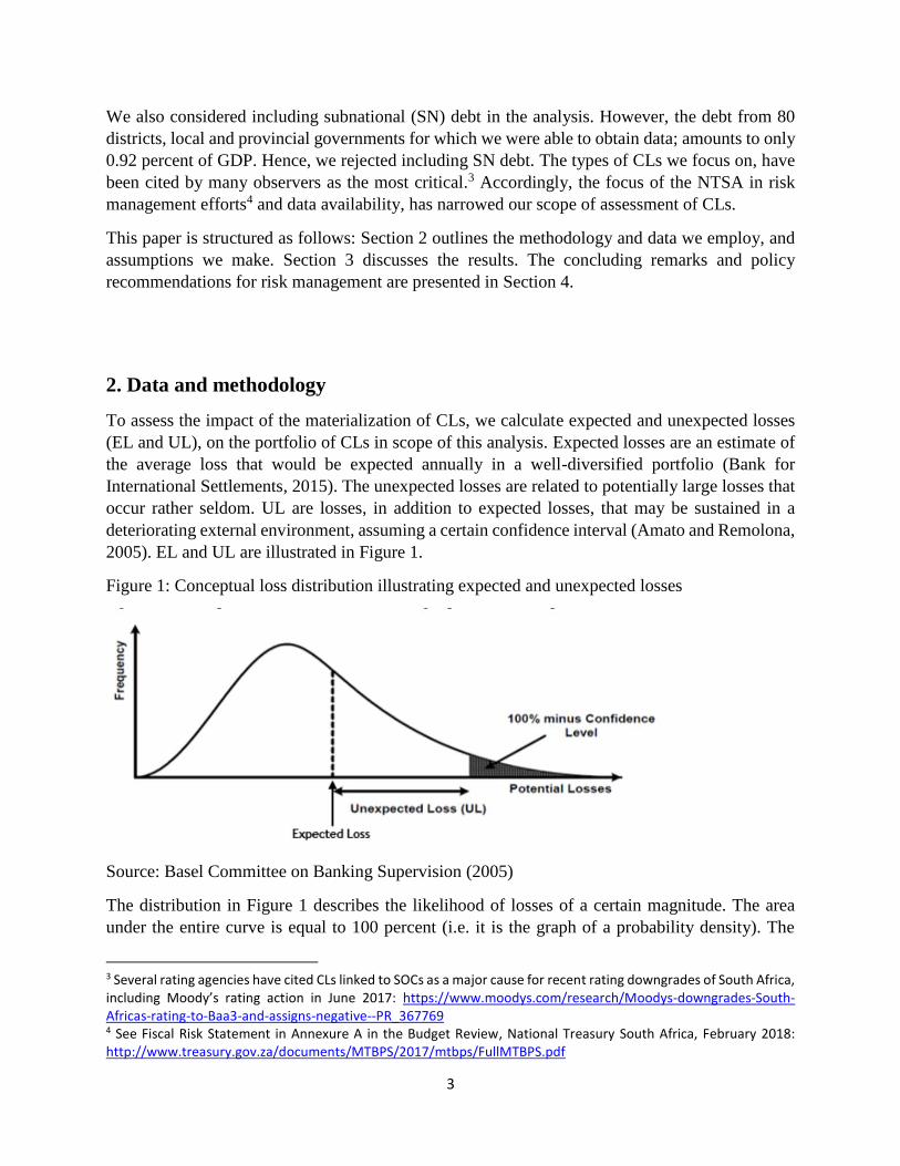
2005). EL and UL are illustrated in Figure 1.

Figure 1: Conceptual loss distribution illustrating expected and unexpected losses

Source: Basel Committee on Banking Supervision (2005)

The distribution in Figure 1 describes the likelihood of losses of a certain magnitude. The area

under the entire curve is equal to 100 percent (i.e. it is the graph of a probability density). The

3 Several rating agencies have cited CLs linked to SOCs as a major cause for recent rating downgrades of South Africa, including Moody’s rating action in June 2017: https://www.moodys.com/research/Moodys-downgrades-South-Africas-rating-to-Baa3-and-assigns-negative--PR_367769 4 See Fiscal Risk Statement in Annexure A in the Budget Review, National Treasury South Africa, February 2018: http://www.treasury.gov.za/documents/MTBPS/2017/mtbps/FullMTBPS.pdf

4

curve shows that small losses around or slightly below EL occur more frequently than large losses.

The likelihood that losses will exceed the sum of EL and UL, equals the shaded area under the

right-hand side of the curve. For example, 100 percent minus this likelihood is called the

confidence level and the corresponding threshold is sometimes called Value-at-Risk (VaR) at this

confidence level, particularly in financial institutions.

We calculate EL on the entity level as the product of: exposure at distress (EAD), the probability

of distress (PD)5 of the respective entities, and loss given distress (LGD). This is presented with

the following formula: 𝐸𝐿 = 𝐸𝐴𝐷 × 𝑃𝐷 × 𝐿𝐺𝐷.

(1)

▪ Exposure at distress is defined as the amount to which the government is exposed to, if an

entity experiences a credit event (i.e. is in distress). Although usually the EAD is defined

as the amount outstanding, for SOCs and the RAF we define it as annual payments to

service liabilities as currently recorded on their balance sheets. We follow this approach

because we assume the government will step-in to undertake payments to creditors in the

case of entities’ distress. Hence, creditors would not accelerate debts. To estimate annual

liability payments for SOCs and the RAF, we obtain the liability stock from their annual

financial statements (see Figure 2). We assume an equal maturity profile of guaranteed and

non-guaranteed liabilities. For government guaranteed debt, from the 2018 Budget Review

of the National Treasury of South Africa; we know that in aggregate SOCs redeem 4.9

percent of the total outstanding debt in FY 2018/19, 5.7 percent in FY 2019/20, and 4.4

percent in FY 2020/21. By accounting for all liabilities, not only for the guaranteed debt,

we assume strong implicit support by the government for the non-guaranteed liabilities as

well. This seems consistent with market data because the observed spread of the non-

guaranteed SOCs’ debt securities and government debt is fairly small. In addition, the

assessment of the credit rating agencies often significantly notching up SOCs’ stand-alone

rating to reflect implicit government support, e.g. (Moody's Investor Service, 2018)). For

IPPs and PPPs, we follow the more conventional approach. In the case of public party

default, we assume the government makes payments equal to the termination values for

these events.6 We use termination values as published by NTSA (National Treasury of

South Africa, 2018).

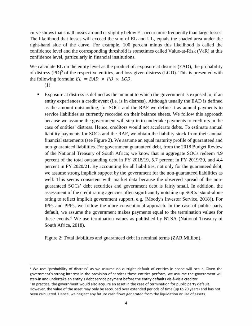
Figure 2: Total liabilities and guaranteed debt in nominal terms (ZAR Million).

5 We use “probability of distress” as we assume no outright default of entities in scope will occur. Given the government’s strong interest in the provision of services these entities perform, we assume the government will step-in and undertake an entity’s debt service payment before the entity defaults vis-à-vis a creditor. 6 In practice, the government would also acquire an asset in the case of termination for public party default. However, the value of the asset may only be recouped over extended periods of time (up to 20 years) and has not been calculated. Hence, we neglect any future cash flows generated from the liquidation or use of assets.

5

Source: respective companies’ websites and authors’ calculations.

▪ Probabilities of distress scores are based on NTSA’s internal risk rating for each institution.

The Asset and Liability Management (ALM) department at NTSA monitors the entities to

which it is exposed to through CLs.7 To assess the credit quality of beneficiary entities,

ALM has developed an internal credit scoring system. To arrive at a credit rating, credit

analysts assess entities on various qualitative and quantitative factors. These include an

assessment of the operating environment, the regulatory framework, management quality,

diversification, profitability, solvency, liquidity, and others. Entities are ordinally ranked

on a scale from 1 (low risk) to 9 (high risk). To arrive at PDs, NTSA then matches its

internal risk ratings with Moody’s rating scale (see Table 1). This allows NTSA to use

default frequency statistics published by Moody’s to estimate PDs for each rating category

(Moody's Investor Service, 2018).

▪ Loss given distress is estimated to be 100 percent for all entities. Hence, we assume that in

the case of distress, NTSA will undertake the full annual payment to service liabilities with

no contributions from beneficiary entities themselves. Furthermore, we do not assume any

recovery of undertaken payments by NTSA in subsequent years. This assumption seems to

be consistent with the experience of many governments which find it difficult to recover

the payments made, either due to the strained financial position of beneficiaries that

necessitated a government step-in in the first place, and potentially institutional

arrangements and policy signals that reduce entities incentive to repay the government after

already having received support.

7 No risk assessment of individual entities will be published here, which is in line with NTSA policy.

(50,000)

50,000

150,000

250,000

350,000

450,000

550,000

Denel DBSA Eskom Landbank Post Office SANRAL Telkom Transnet SAA

Total liabilites and guaranteed debt (in ZAR million)

Guaranteed debt in FY 2016/17 Total liabilities

6

Table 1: Mapping internal risk ratings with Moody’s rating scale in South Africa

Source: National Treasury of South Africa and Moody’s

Table 2: Method to estimate EAD, PD, and LGD by type of CL

Source: Authors.

Next, we calculate unexpected losses to estimate the potential impact of the materialization of CLs

in a negative scenario. We first calculate UL on the entity level and define UL as a loss at one

standard deviation from EL. We assume outcomes to be represented by a binomial distribution. A

binomial distribution represents a binomial experiment with two potential outcomes, in this case

distress and non-distress. The probability of distress is represented by PD, as above when

calculating EL. Assuming a binomial distribution, the standard deviation of PD is

√𝑃𝐷 × (1 − 𝑃𝐷). Exposure at distress and LGD are defined equally as above when calculating

EL. EAD equals either the annual liability payments or the termination values, depending on the

type of the entity (see Table 2), and LGD remains 100 percent. Hence, 𝑈𝐿 = 𝐸𝐴𝐷 ×

√𝑃𝐷 × (1 − 𝑃𝐷) × 𝐿𝐺𝐷. To arrive at total losses if negative scenarios materialize, as it is

assumed here (i.e. at one standard deviation from EL), we add up expected and unexpected losses.

When aggregating entity level UL to the portfolio level, we simply sum them up. We do not

estimate inter-entity correlations, because we do not have sufficient quality of the data to undertake

such an estimation. Hence, we implicitly assume that distress scenarios are perfectly correlated

across entities. If distress scenarios were not perfectly correlated, we would achieve diversification

Type of CL Exposure PD LGD

SOCs Annual liability payments Based on NTSA internal risk rating 100 percent

IPPs Termination values (for public party default) Based on NTSA internal risk rating 100 percent

PPPs Termination values (for public party default) Based on NTSA internal risk rating 100 percent

Road Accident Fund Annual liability payments Based on NTSA internal risk rating 100 percent

7

effects, and portfolio level ULs would be smaller than the sum of entity level ULs. This may

overestimate actual correlations. However, given that all entities’ operations are predominantly

focused in South Africa and mostly in the utility and infrastructure sectors, and all of them are

state-owned, then assuming a strong correlation between them may be reasonable.

This analysis of the impact of CL materialization is based on a number of assumptions:

▪ Any materialization of CLs will increase the borrowing requirement in equal amounts. We

assume that any materialization of CLs requires an equal amount of cash to be provided by

the government in the same year as CLs materialize. Also, we assume the government

raises this amount of cash by engaging in marginal borrowing, not raising additional

revenues or cutting expenditures.

▪ EL and UL are statistical concepts. Given the small portfolio of entities, the short time

horizon (three years), and the potentially significant correlation of distress among entities,

actual outcomes may deviate significantly from our statistical measures. The statistical

measures used may be a much better approximation of the outcomes if the CL portfolio

was large in scope, and well-diversified.

▪ We know the redemption profile of guaranteed SOC debt in aggregate. We do not know

the liability payment schedule for individual entities. We assume that each entity’s liability

payment schedule will exhibit annual payments that are proportional to SOCs’ guaranteed

debt redemptions.

▪ We do not assume new borrowing by entities. Only liabilities currently on entities’ balance

sheets are included in our exposure measures.

▪ We do not distinguish between implicit and explicit government support. We assume

government will step-in to save entities from default of guaranteed and non-guaranteed

liabilities in equal measure.

▪ We only model CLs from the entities in scope (nine SOCs, PPAs to IPPs, PPPs, and RAF).

▪ We rely on NTSA’s internal risk ratings to provide an accurate reflection on credit risk.

▪ We do not account for the potential effect of government taking ownership of assets if CLs

materialize. Particularly, in the case of IPPs, termination may lead to the government taking

ownership of power producers’ assets. These assets may be liquidated over time or generate

revenues. If this was the case, future government revenues may increase and will lower the

borrowing requirements in subsequent years.

The assessment of the impact of the losses from CLs on debt burden indicators and debt dynamics

is done though simulations in the well-established debt sustainability tool designed by the IMF

8

(Market Access Country Debt Sustainability Analysis (MAC DSA))8. The rationale for conducting

the simulations with the MAC DSA tool is because it enables approximate quantification of the

development of debt burden indicators in case when costs related to contingent liabilities

materialize in a consistent macro framework. Accordingly, this tool quantifies how costs arising

from materialization of contingent liabilities will affect the overall gross financing needs,

government debt and debt dynamics of the country in a three-year horizon, by preserving the

consistency in the macro framework. The major novelty in our approach is that we quantify the

annual amounts of expected plus unexpected losses from the possible materialization of contingent

liabilities based on the current probability of distress estimates. Additionally, we include both

explicit and implicit CLs in our analysis.

Box 1: Differences with the IMF approach of quantifying contingent liabilities presented in

Article IV, July 2017

Our approach of quantifying the CLs in South Africa differs substantially from the

methodology applied by the IMF in their latest Article IV for South Africa published in July

2017. Those differences are as follows:

I) Differences in the scope of liabilities included in the calculations: the IMF takes into

account only explicit CLs such as the government guaranteed debt of the SOCs. In our

computations we take the total liabilities (explicitly and implicitly guaranteed) of the

largest SOEs that are much wider than size of the government guaranteed debt.

Furthermore, in our analysis we also include the IPPs which are not included in the IMF

approach.

II) The IMF, in their shock scenario, assumes that all contingent liabilities in scope will

materialize in the first year of the analysis. Furthermore, the IMF assumes all guaranteed

debt will be accelerated and will lead to an equal increase in government debt. Our

approach differs in two respects: First, we assume beneficiary entities only default on

annual liability payments and the government will step-in to undertake these payments.

Hence, creditors would not perceive a default on their loans and credits, and will not

accelerate debt. This assumption seems consistent with past action by the South African

government, aimed at avoiding outright defaults of SOCs and the negative macro-

economic effects. To reflect our assumption, we define exposure at distress to be annual

liability payments, not total liabilities outstanding. Second, we use a risk-based and

statistical approach. The IMF does not differentiate credit quality of various entities. We

do. Based on NTSA’s internal risk ratings, we infer distress probabilities and apply them

8 The MAC DSA tool is developed by the IMF and is regularly used as part of the Article IV reports for the emerging and advanced economies in the world. More details can found on: https://www.imf.org/external/pubs/ft/dsa/mac.htm and the IMF 2013 Staff Guidance Note for Public Debt Sustainability Analysis in Market-Access Countries.

9

to calculate expected and unexpected losses. While the IMF bases their calculations on

the worst case scenario possible (all entities will default in year 1), we construct a scenario

based on expectations (expected losses) and a negative scenario (expected plus

unexpected losses).

The simulations in the MAC DSA template are conducted based on the latest macro, fiscal and

borrowing assumptions presented in the Budget Review from National Treasury by South African

Republic in February 2018 (Table 3). Accordingly, the structure of the new borrowing as a result

of the materialization of the contingent liabilities, preserves the same structure of the stock of debt.

Table 3: Major assumptions used for the MAC DSA template9.

Source: Budget Review, National Treasury South Africa, February 2018

We take the nominal amount for the liability size of the nine largest SOEs from their latest financial

statements published online on the respective companies’ web-sites. As presented in Figure 3, the

total nominal amount of debt summed across all nine SOEs equals 6.2 percent of Nominal GDP,

whereas the nominal amount of their total liabilities equals 20.4 percent.

9 The macro-economic baseline data are by calendar year and they are adjusted to fiscal year data that starts April 1st. This adjustment does not affect the assumptions about the macro data presented in Table 3. The exposure data for CLs are by fiscal year which is consistent with the overall framework. Nevertheless, the adjustment of calendar to fiscal year is not expected to impose distortions because the fiscal year closely overlaps with the calendar year.

2017 2018 2019 2020

Real GDP growth 1 1.5 1.9 2.3

Nominal GDP growth 6.0 7.3 7.2 7.7

Budget balance % of GDP -4.3 -3.6 -3.6 -3.5

Debt-to-GDP ratio 53.3 55.1 55.3 56.0

Short-term domestic

Medeium and long-term domestic

Foreign medium and long-term debt

Structure of the stock of debt (% of total debt stock)

12%

79%

9%

10

Figure 3: Total liabilities and guaranteed debt as a share of nominal GDP.

Source: respective companies’ websites and authors’ calculations.

3. Results

The estimations of the expected and expected plus unexpected losses from CLs in nominal

amounts and as a share of GDP, spread over a three-year horizon, are smooth and not very large

according to the current PD scores (Figure 4). In nominal amounts, they range between ZAR 17.3

billion and ZAR 22.3 billion for the expected losses. Scaled in terms of nominal GDP, they equal

0.4 percent respectively. The estimated nominal amounts of expected plus unexpected losses

ranges between ZAR 30.5 billion and ZAR 40.1 billion, and in terms of nominal GDP are between

0.6 and 0.8 percent, respectively. The estimated amounts of expected plus unexpected losses from

CLs will materialize gradually over the years of projection. Accordingly, their gradual

materialization will constitute a drag on the fiscal policy due to the higher fiscal transfers to the

SOEs, because their access to markets will be restricted. In contrast, in the most recent contingent

liability shock scenario simulated in Article IV published by the IMF in July 2017, the size of the

contingent liability shock is imposed as ZAR 610.4 billion or 12.3 percent of GDP in a single year.

We argue that this shock is not realistic because it assumes that SOEs will actually go bankrupt

and creditors will accelerate all liabilities. As argued, we assume the government will step-in to

undertake periodic debt service payments if entities are in distress, rather than allowing entities to

fail. Hence, a key driver in limiting the size of the CL shock is the long-term repayment schedule

for guaranteed debt (with between four and six percent of the current debt stock being redeemed

annually in the three-year period that we analyze.

-

5

10

15

20

25

Total guaranteed debt (% of GDP) Total liabilites (% of GDP)

Total guarabnteed debt and liabilities as a share of nominal GDP

11

Figure 4: Estimates of expected and expected plus unexpected losses from contingent liabilities -

in nominal terms (left figure) and as a percent of GDP (right figure)10

Source: authors’ calculations based on data from SA treasury, budget bulletins and other national

sources.

In order to assess how the materialization of CLs will affect the annual marginal borrowing

requirements by the government, we compare the major debt burden indicators: debt and gross

financing needs (GFN) to GDP ratios as solvency indicators, and debt service to revenue ratio as

a liquidity indicator. We also compare the debt dynamics decomposition between the baseline

projection and the ones that incorporate the expected plus unexpected losses from CLs. This will

help us to derive conclusions which factors contribute mostly to the debt accumulation.

The development of GFN to GDP ratio, with incorporated expected and expected plus unexpected

losses from CLs, indicates that GFN will be higher by 0.8 percent of GDP until 2020 compared to

the baseline (Figure 5). The GFN will be between 10 and 10.4 percent of GDP by 2020 including

the expected and expected plus unexpected losses from contingent liabilities, respectively,

compared to 9.6 percent with the baseline. This increase of the GFN is a result of increased fiscal

costs triggered by distress of the companies in form of capital and liquidity support, which needs

to be covered by additional borrowing.

10 The macro-economic baseline data are by calendar year and they are adjusted to fiscal year data. This adjustment does not affect the assumptions about the macro data presented in Table 2. The exposure data for CLs are by fiscal year which is consistent with the overall framework. Nevertheless, the adjustment of calendar to fiscal year is not expected to impose distortions because the fiscal year most closely overlaps with the calendar year.

0

5

10

15

20

25

30

35

40

45

2018 2019 2020

Nominal ammounts of expected losses from contingent liabilites

Nominal ammounts of expected and unexpected losses from contingent liabilites

0.0

0.1

0.2

0.3

0.4

0.5

0.6

0.7

0.8

0.9

2018 2019 2020

Expected losses from contingent liabilites as a share of GDP

Expected and unexpected losses from contingent liabilites as a share of GDP

12

Figure 5: GFN to GDP ratio

Source: Authors’ calculations based on data from Budget Review, National Treasury South Africa,

February 2018and other national sources.

The projected debt trajectory indicates that in cumulative terms, debt to GDP ratio will increase

by 1.2 and 2.1 percent of GDP by year 2020 for the expected and expected plus unexpected losses,

respectively. Accordingly, the debt to GDP ratio will reach between 57.1 and 58 percent in 2020

compared to the baseline projection of debt-to-GDP ratio of 56 percent (Figure 6). Although the

increase of the debt-to-GDP ratio is not large according to the two scenarios of contingent

liabilities, what is most concerning is that debt level as a share of GDP has a tendency of growing

further and will be harder to stabilize, compared to the baseline projection where debt stabilizes.

In order for the debt level as a share of GDP to stabilize with the contingent liability shock

scenarios, either GDP growth needs to be higher than the baseline scenario, and/or the government

needs to run lower budget deficits than predicted in the baseline and/or the new borrowing needs

to be done by lower interest rates. Nevertheless, all of these options would not be feasible in the

case contingent liabilities materialize because markets’ confidence will deteriorate and risk

aversion of the markets will increase.

Figure 6: Debt to GDP ratio

Source: Authors’ calculations based on data from Budget Review, National Treasury South Africa,

February 2018 and other national sources.

9

10

11

12

2017 2018 2019 2020

Gross financing needs to GDP ratio

GFN to GDP ratio - baseline projection

GFN to GDP ratio - expected losses from contingent liabilites

GFN to GDP ratio - expected and unexpected losses from contingent liabilites

52

53

54

55

56

57

58

59

2017 2018 2019 2020

Debt to GDP ratio

Debt to GDP ratio - baseline projection

Debt to GDP ratio - expected losses from contingent liabilites

Debt to GDP ratio - expected and unexpected losses from contingent liabilites

13

The liquidity indicator: debt service to revenue ratio, shows increase of debt service between 0.5

and 0.8 percentage points of revenues by 2020, for the expected plus unexpected losses of

contingent liabilities compared to the baseline (Figure 7). Accordingly, the debt service to revenue

ratio is expected to reach between 32.9 and 33.2 percent by 2020, compared to 32.5 percent with

the baseline projection.

Figure 7: Debt service to revenue ratio

Source: Authors’ calculations based on data from Budget Review, National Treasury South Africa,

February 2018and other national sources.

The final part of this analysis discusses the differences in the debt dynamics between the baseline

projection and the ones that incorporate the expected plus unexpected losses from contingent

liabilities. As presented in Figure 8, the major noticeable difference is that, in the simulations that

incorporate the CLs, one of the significant drivers of debt accumulation will be the losses from

materialization of contingent liabilities.

32

33

34

35

36

37

2017 2018 2019 2020

Debt service to revenue ratio

Debt service to revenue ratio - baseline projection

Debt service to revenue ratio - expected losses from contingent liabilites

Debt service to revenue ratio - expected and unexpected losses from contingent liabilites

14

Figure 8: Debt dynamics decomposition – baseline scenario (top figure), expected losses from

contingent liabilities (middle figure), expected plus unexpected losses from contingent liabilities

(bottom figure).

-6

-4

-2

0

2

4

6

8

2008 2009 2010 2011 2012 2013 2014 2015 2016 2017 2018 2019 2020

Debt-Creating Flows

Primary deficit Real GDP growth

Real interest rate Exchange rate depreciation

Other debt-creating flows (including contingent liabilities in the projected period)* Residual includes exchange rate changes in the projected period

Change in gross public sector debt

projection(in percent of GDP)

-5

-3

-1

1

3

5

7

9

11

cumulative

-6

-4

-2

0

2

4

6

8

2006 2007 2008 2009 2010 2011 2012 2013 2014 2015 2016 2017 2018 2019 2020

Debt-Creating Flows

Primary deficit Real GDP growth

Real interest rate Exchange rate depreciation

Other debt-creating flows (including contingent liabilities in the projected period)* Residual includes exchange rate changes in the projected period

Change in gross public sector debt

projection(in percent of GDP)

-5

-3

-1

1

3

5

7

9

11

cumulative

15

*Other debt creating flows, apart from including the contingent liabilities, also include

privatization receipts and other stock-flow adjustment. In the past period, they include mostly

privatization receipts, whereas in the projected period they include dominantly contingent

liabilities.

Source: authors’ calculations based on data from Budget Review, National Treasury South Africa,

February 2018, IMF Article IV July 2017 and national sources.

The materialization of the losses from the contingent liabilities will become a significant factor

that will drive the debt accumulation in the medium-term future. Furthermore, these losses will be

even higher if the overall macro and financial conditions deteriorate in South Africa compared to

the baseline and also if the financial strength of the analyzed companies weakens for any other

reason. This urges the issue of required remedial measures by the government that will be

discussed in the next section.

4. Conclusions and policy implications

This analysis has quantified the losses from materialization of contingent liabilities and

incorporated in the debt dynamics in South Africa from specific sectors of the economy by utilizing

PD scores. The results indicate that the solvency and liquidity situation in the country may

deteriorate if the contingent liabilities materialize. The solvency and liquidity deterioration in the

country may be more severe if the contingent liability shock is much stronger than what is

estimated with the PD scores. Ultimately, the current estimates suggest that CLs may constitute a

drag to fiscal policy in medium term. Gradual materialization of CLs would require further fiscal

effort to keep debt sustainable as the current estimates suggest limited cost per year that may

-6

-4

-2

0

2

4

6

8

2008 2009 2010 2011 2012 2013 2014 2015 2016 2017 2018 2019 2020

Debt-Creating Flows

Primary deficit Real GDP growth

Real interest rate Exchange rate depreciation

Other debt-creating flows (including contingent liabilities in the projected period)* Residual includes exchange rate changes in the projected period

Change in gross public sector debt

projection(in percent of GDP)

-5

-3

-1

1

3

5

7

9

11

cumulative

16

accumulate in medium-term and long-term. Their gradual accumulation in long-term future may

jeopardize the debt sustainability of the country.

Largest deterioration will occur in the debt to GDP ratio. The debt accumulation, including the

expected plus unexpected losses from contingent liabilities, will be higher by 2.1 percentage points

of GDP within three years, compared to the baseline projection. What is more concerning is that

the debt level will be more difficult to stabilize if the contingent liabilities materialize, which is

not the case with debt trajectory in the baseline. The losses incurred from the contingent liabilities

may become significant driving factor of debt accumulation in medium term future.

Nevertheless, the results of this analysis should be taken with caution, having in mind the

limitations of the quantitative approach conducted. For example, the MAC DSA template works

mostly in partial equilibrium where it analyzes the impact of one factor, while it keeps other factors

unaffected. In this case, the materialization of CLs does not assume lower GDP growth, higher

interest rates and exchange rate depreciation as could be the case if they materialize in reality.

Another limitation of this analysis is that it is focused on narrow area of assessment of CLs. For

instance, it does not include the financial sector that is large in South Africa and related to almost

any other sector in the economy. CLs originating from the financial sector may trigger significantly

higher losses beyond those modeled here.

Overall, this analysis, regardless of the size of the CL shock, urges for remedial measures and

building protective buffers in the case CLs materialize, which may happen in the medium-term

future. We commend NTSA for recent actions taken to strengthen CL risk management, including

improving risk assessment, the publication of a fiscal risk statement, and reform initiatives to

improve SOC governance. Based on international sound practice, further risk management tools

may be considered (Bachmair, 2016). On a portfolio level, limits may be set on the flow or stock

of exposure, such as a limit on guarantee issuance relative to economic aggregates. For individual

guarantee agreements, NTSA may implement specific eligibility criteria (e.g. a minimum credit

rating, or no arrears with government) before a guarantee can be issued. NTSA may also charge

risk-based fees to entities to compensate for (part of) the support government is providing. Fees

could be based on the economic value of a guarantee. Expected and unexpected losses estimated

in this note can discounted to the time of guarantee issuance and applied as a proxy for the value

of a guarantee. To reduce fiscal volatility, the government may consider designing a contingency

reserve account as a buffer for potential materialization of CLs. We acknowledge that a strained

fiscal stance increases the political will required to implement such an account. Resources in the

reserve account may be generated from fees, budget provisions, investment income, etc. A reserve

account may be actual or notional. In an actual account, the government would set up a fund and

manage these funds. In a notional account, funds in the account may be used to pay down

government debt. An example of notional account, as used in Sweden, requires a high degree of

budgetary discipline, to ensure resources in the fund are not used for competing budgetary

expenditures. Furthermore, monitoring, account for, and reporting of risks is an important function.

The government will have to decide what information is published or used only for internal

purposes (e.g. risk reporting on a portfolio level may be appropriate for publication, while risk

17

assessment of individual entities may not). All these risk mitigation and monitoring measures

tackle the proximate causes of contingent liabilities. The ultimate cause may lie in the performance

of SOCs themselves. Initiatives to ensure sustainable profitability of SOCs may hold the key to

reducing CLs. These initiatives can include corporate governance reform, financial management

reform, and regulatory and sector reforms.

18

References

Amato, J., and Remolona , E. (20005). The Pricing of Unexpected Credit Losses. BIS Working

Papers.

Bachmair, F. F. (2016). Contingent Liabilities Risk Management. World Bank Policy Research

Working Paper.

Bank for International Settlements. (2015). Guidance on credit risk and accounting for expected

credit loss. Basel Committee on Banking Supervision.

Basel Committee on Banking Supervision. (2005). An Explanatory Note on the Basel II IRB

Risk Weight.

International Monetary Fund. (2016). Analyzing and managing fiscal risks - best practices.

International Monetary Fund. (2017). Article IV South Africa, IMF Country Report No. 17/189,

July 2017.

Moody's Investor Service. (2018). Annual Default Study: Corporate Default and Recovery Rates,

1920 - 2017.

Moody's Investor Service. (2018). Rating Action: Moody's downgrades Eskom's ratings to

B2/B3/Ba2.za NSR; negative outlook. Global Credit Research.

National Treasury of South Africa. (2017). Credit Risk Revue of Government Explicit

Contingent Liabilities.

National Treasury of South Africa. (2018). Budget Review.