econstorMake Your Publications Visible.

A Service of

zbwLeibniz-InformationszentrumWirtschaftLeibniz Information Centrefor Economics

Su, Biwei; Heshmati, Almas

Working Paper

Analysis of the determinants of income and incomegap between urban and rural China

IZA Discussion Papers, No. 7162

Provided in Cooperation with:IZA – Institute of Labor Economics

Suggested Citation: Su, Biwei; Heshmati, Almas (2013) : Analysis of the determinants of incomeand income gap between urban and rural China, IZA Discussion Papers, No. 7162, Institute forthe Study of Labor (IZA), Bonn

This Version is available at:http://hdl.handle.net/10419/69459

Standard-Nutzungsbedingungen:

Die Dokumente auf EconStor dürfen zu eigenen wissenschaftlichenZwecken und zum Privatgebrauch gespeichert und kopiert werden.

Sie dürfen die Dokumente nicht für öffentliche oder kommerzielleZwecke vervielfältigen, öffentlich ausstellen, öffentlich zugänglichmachen, vertreiben oder anderweitig nutzen.

Sofern die Verfasser die Dokumente unter Open-Content-Lizenzen(insbesondere CC-Lizenzen) zur Verfügung gestellt haben sollten,gelten abweichend von diesen Nutzungsbedingungen die in der dortgenannten Lizenz gewährten Nutzungsrechte.

Terms of use:

Documents in EconStor may be saved and copied for yourpersonal and scholarly purposes.

You are not to copy documents for public or commercialpurposes, to exhibit the documents publicly, to make thempublicly available on the internet, or to distribute or otherwiseuse the documents in public.

If the documents have been made available under an OpenContent Licence (especially Creative Commons Licences), youmay exercise further usage rights as specified in the indicatedlicence.

www.econstor.eu

DI

SC

US

SI

ON

P

AP

ER

S

ER

IE

S

Forschungsinstitut zur Zukunft der ArbeitInstitute for the Study of Labor

Analysis of the Determinants of Income andIncome Gap between Urban and Rural China

IZA DP No. 7162

January 2013

Biwei SuAlmas Heshmati

Analysis of the Determinants of

Income and Income Gap between Urban and Rural China

Biwei Su Korea University

Almas Heshmati

Korea University and IZA

Discussion Paper No. 7162 January 2013

IZA

P.O. Box 7240 53072 Bonn

Germany

Phone: +49-228-3894-0 Fax: +49-228-3894-180

E-mail: iza@iza.org

Any opinions expressed here are those of the author(s) and not those of IZA. Research published in this series may include views on policy, but the institute itself takes no institutional policy positions. The IZA research network is committed to the IZA Guiding Principles of Research Integrity. The Institute for the Study of Labor (IZA) in Bonn is a local and virtual international research center and a place of communication between science, politics and business. IZA is an independent nonprofit organization supported by Deutsche Post Foundation. The center is associated with the University of Bonn and offers a stimulating research environment through its international network, workshops and conferences, data service, project support, research visits and doctoral program. IZA engages in (i) original and internationally competitive research in all fields of labor economics, (ii) development of policy concepts, and (iii) dissemination of research results and concepts to the interested public. IZA Discussion Papers often represent preliminary work and are circulated to encourage discussion. Citation of such a paper should account for its provisional character. A revised version may be available directly from the author.

IZA Discussion Paper No. 7162 January 2013

ABSTRACT

Analysis of the Determinants of Income and Income Gap between Urban and Rural China

This paper studies on the determinants of income and urban-rural income gap to shed light on the problem of urban-rural income inequality in China. OLS, conditional quantile regression and Blinder-Oaxaca decomposition methods are used to analyze four waves of the China Health and Nutrition Survey (CHNS) household data. Results show that education and occupation are essential determinants of households’ income level. These two factors exert heterogeneous effects at different percentiles of the income distribution. In urban areas, education is more valued for high income earners, while for rural areas, specialized or tertiary education are more beneficial for the poorer households. Among all occupational types, farm activities show much lower returns than other types; and this is more evident for individuals at the left tail of the income distribution. We also find that for the sampled provinces, urban-rural income gap increases from the year of 2000 to 2004 but the gap decreases from 2004 to 2009. The income gap can be largely explained by the individuals’ attributes, especially by level of education and type of occupation. JEL Classification: O15, O18, D31, D63, C31 Keywords: urban-rural income gap, Oaxaca-Blinder decomposition, quantile regression,

CHNS household data, China Corresponding author: Almas Heshmati Department of Food and Resource Economics College of Life Sciences and Biotechnology Korea University East Building Room #217 Anam-dong Seongbuk-gu Seoul 136-713 Korea E-mail: heshmati@korea.ac.kr

1. Introduction China has kept a remarkable economic growth path ever since its ice-breaking reform and opening up in 1970s. The nearly two-digit average growth rate for the past three decades not only makes China the world’s fastest-growing major economy but also helps China to lift hundreds of millions people out of poverty. The poverty rate reduced from 85% in 1981 to 16% in 20051 (World Bank, 2008). However, even though there are dramatic improvements in the average living standards of Chinese citizens, the income inequality, especially between urban and rural areas, is significant and expanding. In fact, among developing and transition nations, China is the country with the greatest and most visible set of challenges relating to the issues of urban-rural inequality.

Economic growth in developing and transition nations usually has a positive relationship with income inequality (Heshmati, 2007a). A question has been raised that is the increase in inequality an uncomfortable but otherwise innocuous price to pay when the rising tide is raising all boats? Not necessarily, as we account of more than half of the total population in China are rural residents and most of them live underprivilege. Increasing of the income inequality may imperil social stability; hinder the economic growth; and leave the poor even harder to step out their misery. Tackling the distribution-related issue became an important part of China’s government policy in 2002 when the urban-rural income ratio reached over 3.00 for the first time accruing to National Bureau of Statistics of China (2003). The addressed issues included slumping peasant income, heavy tax burdens in rural areas, redistribution of income and development of social safety nets. Administrative measures were put in place at then, which resulted in a sudden rapid expansion. But still, the urban-rural ratio has lingered around 3.00 for recent years, which is extremely high by international standards.

It comes therefore as no surprise that we are interested at the causing factors behind the income inequality. We achieve this by studying the determinants of household’s income and how those factors contribute to the income gap. The analysis has been conducted in the following steps. We firstly use the classical ordinary least square (OLS) regression to estimate the Mincerian income equation. Even though the computational tractability of OLS estimator is very appealing, it cannot uncover the effects of independent variables on the “shape” of distribution. To cope with this, we apply the conditional quantile regression developed by Koenker and Bassett (1978). Unlike OLS, it provides regression curves corresponding to the various points of income distribution. Last, we refer to the Blinder-Oaxaca decomposition method to explore to what extent the urban-rural income gap can be explained by household heads individual characteristics.

This paper proceeds as follows. Section 2 reviews and summarizes relevant literatures about the studies on income inequality in China. Section 3 introduces the data and the variables that we used in this research. Section 4 provides models and methodologies for our estimation. Section 5 analyzes the results. Section 6 contains the summary of the major findings and policy suggestions.

1 Poverty is defined by the World Bank as the number of people living on < $1.25 per day.

2. Literature Review Since the early 1990s, income inequality in China has been under scrutiny both at home and aboard. The widen inequality has been studied at four different levels: within rural areas, within urban areas, between urban and rural areas and last, at national or regional level as a whole.

Many studies reached the consensus that income inequality within rural and urban areas gone up during the transition period (Khan and Riskin, 1998; Knight and Song, 2003; Benjamin et al. 2005; Heshmati, 2007b, among others). Despite the upward trend, due to several effective reforms in rural areas, there were slight declines in rate of poverty over time. Yang and Zhou (1999) found urban-rural inequality was initially narrowed following the success of policy aiming to reduce rural-urban division, such as increases in procurement prices for agricultural products, adoption of household responsibility systems, liberalizing local markets, and the relaxation of restrictions on labor mobility to cities. But the income gap widened again after 1985 because of the higher labor productivity in urban state-owned industries than that in rural industries and agricultural sector. Johnson (2001) found a decline of urban-rural income ratio from 1994 to 1997, but an increase after 1997. Several scholars studied about the overall income inequality in China and attributed it to inequality within and between urban and rural areas. Yang (1999), by analyzing Gini ratios and generalized entropy measures in two provinces for four years between 1986 and 1994, found that urban-rural inequality contributes to about 80% of the overall inequality. Wu and Perloff (2005) analyzed income distribution from 1985 to 2001 and argued that urban-rural gap played an increasing important role to enlarge income inequality among other factors. The seriousness of urban-rural income inequality has also been proved by Kanbur and Zhao (1999), Lin et al. (2002), Heshmati (2004), and Yao et al. (2005), and others.

On the other hand, numerous studies intended to find the underlying causing factors of increased income inequality. Here we list several of them that have been proposed, tested and examined most frequently. The first factor is the political strategies that favored heavy-industry in the early stage and manufacturing sectors later on. Investments, preferential policies, and financial supports stimulated the growth in urban areas. Agricultural sector was lagged behind and used as the foundation for developing other sectors. Agricultural surplus was extracted for urban capital accumulation and urban-based subsidies. Main enforcement mechanisms such as the state control of agricultural production and procurement, the suppression of food-staple prices, and restrictions on rural-urban migration via the Hukou system largely deteriorated the income for rural residents (Yang, 1999; Yang and Zhou, 1999; Kanbur and Zhang, 2005).

The second factor is the progress of urbanization through the influx of rural people into cities. Murphy (2002) praised that the rural-urban migration allowed flows of people, skills, capital, commodities and information and therefore contributed to the urban-rural income. Using the 1995 survey data, Li (2009) suggested that rural migration made a contribution to the growth of rural income, not only by raising labor productivity of migrant workers but also by permitting more efficient allocation of remaining, non-migrating workers. The urban-rural income gap might be improved by urbanization.

The third reason might be the development of financial sectors. Greenwood and Jovanovic (1989) studied the nexus relationship among economic growth, income

distribution and financial structure in a dynamic model. They found an inverse U-shape relationship between financial development and income distribution. In case of China, Zhang (2004) took ratio of bank credit over GDP as the financial intermediary and found that the evolution of financial intermediary significantly enlarged urban-rural income gap at provincial level from 1978 to 1998. Yao (2005) found positive and bilateral Granger causality lay between financial development dimension and urban-rural income gap, but negative and bilateral Granger causality existed between financial development efficiency and urban-rural income gap.

Fourth, despite the governing party has emphasized that growth would solve distribution problems through a trickle-down effect across the regions and social strata, it did not occur automatically. On the contrary the prosperity in the urban areas further increased this inequality. The effort to transform China as a whole into a market economy ran into obstacles rooted in conflicts between state industry and staple agriculture (Putterman, 1992). Dual economy structure has not been changed but it was been strengthened during the economic reform and the uneven growth rate between the two sectors enlarged the income inequality.

Fifth, some scholars addressed the issue from the perspective of human capital. In light of endogenous growth theory, Guo (2005) tried to use human capital, the birth rate and their interaction to observe and analyze the urban-rural income gap in China. He revealed that Malthusian homeostasis in rural areas caused a high birth rate and low rate of human capital accumulation decisively impedes the growth of peasants’ income, while the urban sectors have entered a more equilibrated stage of sustainable growth, for a paradigm of a low birth rate and high human capital stock and accumulation.

Finally, the effect of China’s opening up on urban-rural income inequality is far from conclusive. Wei and Yi (2001) studied around 100 cities in China and found that opening up reform actually narrowed the rural-urban income gap. Similarly, Hertel and Fan (2006) argued that along with WTO accession, the combined impact of product and factor market reforms largely reduced rural-urban income inequality. On the contrary, Jeanneney and Hua (2008) studied the impact of exchange rate policy on urban-rural per capita income and found that real appreciation attenuated inequality, whereas real depreciation accentuated inequality. Using the provincial panel data from 1978 to 2007, Wei and Zhao (2012) proved that international trade played a key role in forming the increasing urban-rural gap through effects of employment and wage.

In sum, existing studies on the issue of urban-rural income inequality generally focus on factors that are closely related to economic transformation especially during the periods in the 1980s and 1990s. Rather than examine income inequality using those factors that mentioned, we look at this issue from the aspect of individual characteristics, trying to find how one’s age, education level, occupation, marital status, registration type affect urban or rural residents’ income level respectively; and how those factors contribute to the income gap. Moreover, we use the household survey data from 2000 to 2009, covering a time span that has not been fully studied yet, and therefore enabling us to provide the latest information about the state of urban-rural income inequality in China.

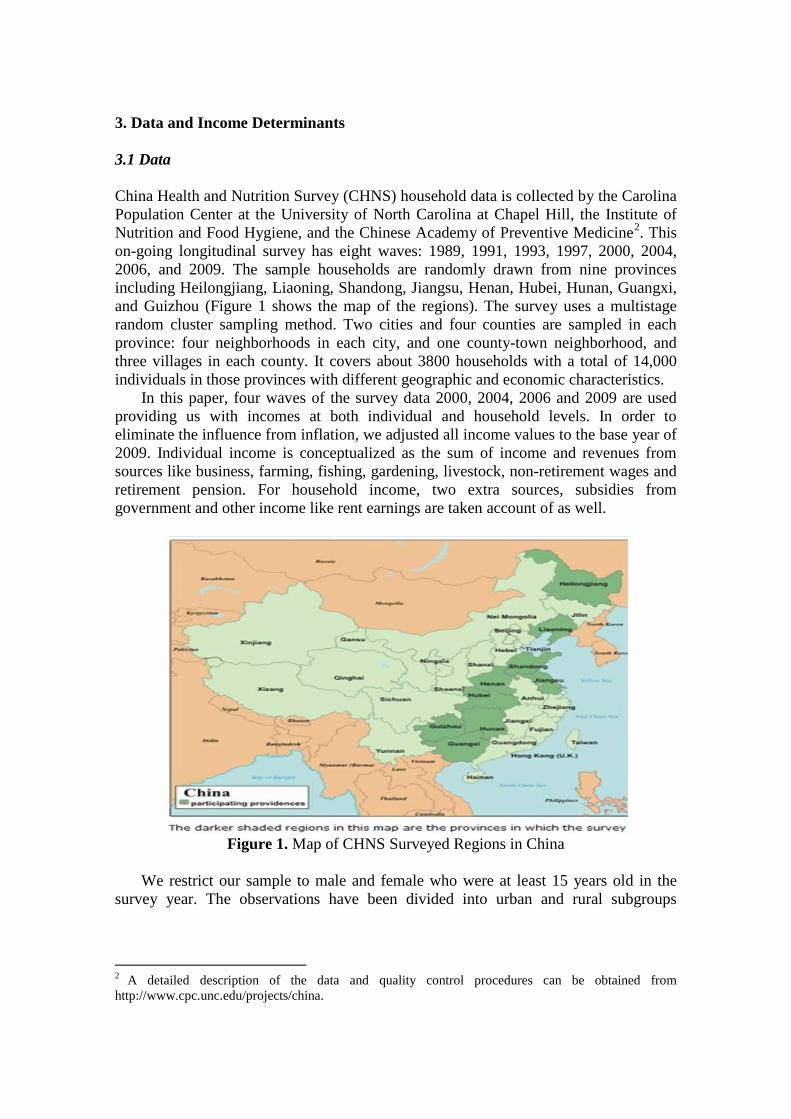
3. Data and Income Determinants 3.1 Data China Health and Nutrition Survey (CHNS) household data is collected by the Carolina Population Center at the University of North Carolina at Chapel Hill, the Institute of Nutrition and Food Hygiene, and the Chinese Academy of Preventive Medicine2. This on-going longitudinal survey has eight waves: 1989, 1991, 1993, 1997, 2000, 2004, 2006, and 2009. The sample households are randomly drawn from nine provinces including Heilongjiang, Liaoning, Shandong, Jiangsu, Henan, Hubei, Hunan, Guangxi, and Guizhou (Figure 1 shows the map of the regions). The survey uses a multistage random cluster sampling method. Two cities and four counties are sampled in each province: four neighborhoods in each city, and one county-town neighborhood, and three villages in each county. It covers about 3800 households with a total of 14,000 individuals in those provinces with different geographic and economic characteristics.

In this paper, four waves of the survey data 2000, 2004, 2006 and 2009 are used providing us with incomes at both individual and household levels. In order to eliminate the influence from inflation, we adjusted all income values to the base year of 2009. Individual income is conceptualized as the sum of income and revenues from sources like business, farming, fishing, gardening, livestock, non-retirement wages and retirement pension. For household income, two extra sources, subsidies from government and other income like rent earnings are taken account of as well.

Figure 1. Map of CHNS Surveyed Regions in China

We restrict our sample to male and female who were at least 15 years old in the

survey year. The observations have been divided into urban and rural subgroups

2 A detailed description of the data and quality control procedures can be obtained from http://www.cpc.unc.edu/projects/china.

according to the one’s registration type 3 --- Hukou. Table 1 shows the number of individual observations for each sampled year.

Table 1. Number of observations Individual Level 2000 2004 2006 2009 Urban 2562 2080 2086 2258 Rural 6359 4963 4739 5062 Total 8921 7043 6825 7320

3.2 Income Determinants The choice of explanatory variables (listed in Table 2) is guided both by the economic theory and by the empirical context. The standard variables taken to determine one’s income level are the educational level and occupational type. To capture the effect of education, dummy variables are used corresponding to one’s educational attainment, which include no education, primary school, junior high school, senior high school, technical school, and university and above. From Table 3, we can see that generally, urban residents are better educated than rural ones. On average more than 20% of rural residents have no access to education; even for those who are able to attain education, most of them only manage to finish junior middle school level of education. However, the situation is quite different for the urban group. Around 90% of urban residents are educated and over 50% of them are able to attain more than 9 years of education.

With respect to occupation, dummy variable are included corresponding to seven occupational groups --- senior professionals, junior professionals, self-employed businessmen, office staffs, low-paid labors/service workers, agricultural workers (such as peasant, fisherman, hunter) and people who are retired. From Table 3 we note that, more than 60% of rural population is engaged in agricultural-activities and around 10% of rural people works as labor or service worker. Unlike the rural group, urban residents have been distributed more evenly by the occupational type. The retired group contains more than 25% of the urban residents, which is the largest group. It constitutes women over age of 55 and men over 60. And one should notice that even they are classified as retired worker, many of them still take part-time job or operate self-employed businesses. Junior professional such as nurse, technical skill, is the second largest occupation type, followed by self-employed businessman, low paid labor and service worker. The proportions for senior professional and office staff are similar which fluctuated around 10%. And without surprise, only very few urban residents are associated with farm-activities which is no more than 5% of the total urban population.

In addition to the above explanatory variables, a number of background and demographic variables are included in the analysis. First, the experience reflected by the age of the person less than pre-school and years is included. Two variables are used: age (in years), and age-squared to reflect the non-linear effects of age on the income level. Generally, in our sample, rural residents are younger than the urban ones. Second, the effect of household size on the income level is incorporated, as previous study have noted a negative relationship between income and the size of the household (Lipton and Ravallion, 1994). In Table 3, we find a larger family size in rural areas and a decrease in the family size over time for both rural and urban areas. Third, a dummy is added for gender, as numerous researches have suggested that the existence of the gender income

3 We group the households according to the registration type of the head of each family.

gap (Macpherson and Hirsch, 1995; Hughes and Maurer-Fazio, 2002; Wang and Cai, 2006; among others). Forth, effects of marital status and the influence are captured by three dummy variables: single, married and divorced. And having children is also one of our considerations. Last, to account for regional heterogeneity, we add dummy variables where Liaoning is selected as the reference group. 4. The Methodologies and Models In this part, we use ordinary least squares (OLS) and quantile regression methods to estimate the effects of personal characteristics on individual’s annual income for urban and rural residents respectively. The individual level data is used for the purpose. The standard model is based on the human capital earnings function developed by Mincer (1994):

(1) iii XINC εβ +=ln

where lnINCi is the natural logarithm of the annual income for observation i, and Xi is a vector of individual characteristics including a measure of education, age, occupation, gender, marital status, child status, and household size. β is the vector of unknown parameters to be estimated, and εi is a random disturbance term which is assumed to satisfy the usual properties of mean zero and constant variance.

Classical linear regression is a method of estimating conditional mean functions by minimizing sums of squared residuals. Similarly, in conditional quantile regression we use an optimization of a piecewise linear objective function of residuals. We specify equation (1) under conditional quantile regression:

(2) τττ εβ ,')|ln( iiii XXINCQ +=

where Qτ ln(INCi|Xi) is suggesting to estimate the Mincerian earning model at τ-th quantile (Qτ) of the distribution of the dependent variable (Y) conditional on the value of X. Following Koenker and Bassett (1978), the income of an individual is in the τ-th quantile if his income is higher than the proportion τ of the reference group of individuals and lowers than the proportion (1-τ). βτ is the estimated parameter for each explanatory variable correspondingly. Other notations remain the same meaning as they are indicated in equation (1).

Assuming that the τ-th quantile of error term conditional on the regressors is zero ( 0)( , =ii xuQ ττ ), then the τ-th conditional quantile of yi with respect to xi can be written as:

(3) ττ βix')( =ii xyQ

Using median regression method, also known as the sum of absolute deviation (LAD) estimator, we minimize the sum of absolute residuals with symmetrical and asymmetrical weighting systems. The parameter vector βτ can be estimated by:

(4) ∑ −=

∑ −−+∑ −=

∈

∈ ≥∈≥∈

))((argmin

)'()1()'(argminˆ

,

Rβ

Rβ

k

k '|'|

ττ

τ

τ

τ

τ

βξρ

βτβτβ

τ

τ ββτ

ii

ii

ii

ii

ii

xy

xyxyxyiixyii

where the function ρτ(.) is the absolute value function that yields the τ-th sample quantile and ξ(xi, β) is the linear function of parameters. In this study, we are using bootstrapping method to estimate the earning equation for different quantile values of τ (5, 25, 50, 75, and 95) for both urban and rural residents.

Another main objective of this paper is to analyze the composition of the urban-rural income gap. The procedure developed by Oaxaca and Blinder (1973) splits the total income gap into two components: that part of the gap is attributable to differences in observable productive characteristics, and the residual gap is attributable to differences in the returns to the examined characteristics for urban and rural areas.

More specifically, the total urban-rural income gap is equal to:

(5) 1−=r

u

INCINC

D

where, INCu/INCr is the observed urban-rural income ratio. Taking the logarithm form of equation (5) and combining the OLS estimated result of equation (1), the urban-rural income gap can be expressed as:

(6) rruuru XXINCINCD ββ ˆˆlnlnln −=−=

where uINCln and rINCln are the mean values of the natural log of urban and rural annual income respectively. uX and rX are vectors of the mean values of the urban

and rural residents’ productive characteristics. uβ and rβ are vectors of the estimated regression coefficients from separated regressions.

Following Oaxaca (1973), the above equation can be further transformed for decomposition purpose as:

(7) )ˆˆ]()([]ˆ)(ˆ)[(ln rurururu XIXIXXD ββββ −Ω+Ω−+Ω−+Ω−=

where, I is an identity matrix and Ω is a diagonal matrix of weights. This states that the mean difference in log annual income is decomposed into two parts. The first expression on the right hand side is the portion of the income gap attributable to differences in average productive characteristics of urban and rural residents. The difference in the mean characteristics is multiplied by the weighted estimated coefficient from both regressions. Those coefficients are interpreted as the income structure for each individual. The second expression on the right is that portion of the income gap attributable to differences in the rural and urban regression coefficients; that is, difference in the returns to urban and rural residents for same productive characteristics. The latter component is usually regarded as discrimination and the effects of other omitted factors.

Here following the tradition, we adopt Reimers’s (1983) method where Ω=0.5I where I is an identity matrix. The income gap in (7) is reduced to:

(8) ]ˆˆ)[(5.0)ˆˆ]([5.0ln fmfmfmfm XXXXD ββββ −+++−=

5. Analysis of the Results 5.1 OLS estimation Table 4 shows the results for OLS estimation for urban and rural sample groups respectively over the period of 2000 to 2009. The adjusted R-square is around 0.21 to 0.33 suggesting that our regressions explain around 21% to 33% variation of the annual income. The R-square value tends to be low in Mincerian model as it has been shown in many other literatures (Blinder, 1973; Hughes and Maurer-Fazio, 2002; Sicular et al., 2007). This may be because (i) the individual incomes has a large dispersion so that makes regressions difficult to capture the marginal effects of each variable; (ii) there might be some unobserved effects that we fail to capture using the selected variables such as ability. Nevertheless, those regressions shed lights on how the demographic characteristics affect one’s income over time.

It is generally hold that there are significant regional differences (Lin, et al., 2002; Sicular et al. 2007) in China due to biased policies and geographic variations. However, this regional effect seems less significant in our case. This may be due to the fact that the CHNS survey excludes the municipalities like Beijing, Shanghai and Tianjin, places with much higher economy size than other parts of China. Thus, the differences between our sample provinces are moderate. One exception is Jiangsu province, which has a much higher positive influence on personal income compared with the reference group Liaoning and other provinces. Though both Jiangsu and Liaoning are coastal provinces, the former has a 34.4% (urban) and 11.2% (rural) higher income than that for the latter in 2000, and this superiority has been kept till 2009, with 16.0% more income for urban group and 42.9% for rural group. Jiangsu owns its economic development due to its location at the Yangtze River Delta, the largest concentration of adjacent metropolitan areas in China. Rapid development makes it to have the highest GDP per capita and second highest GDP among of all the provinces4 since 2009. But clearly, rapid developments in urban area have also taken place in other provinces, as the results show the gap between Jiangsu and other provinces shrinks.

For the rural area, regional differences become more significant in 2009 than that in 2000. Rural residents’ income in Jiangsu also overtakes rural people’s income in other provinces thanks to the rapid reform and innovation as well as the agricultural modernization in its rural areas. The rural income gap between Jiangsu and Liaoning province from 2000 to 2009 is enlarged by 30%. The income gap between Jiangsu and the least developed province Henan within rural areas in 2009 is nearly 60%. In sum, in recent 10 years, regional income differences become more significant in rural areas.

Education is one the factors that we are most interested in. We define people who have received no education as the benchmark and define other five educational categories. According to the results, education is positively related to one’s income and those educational returns are higher among the urban residents. This can be explained that economic development and capital accumulation have been taken place more intensively in the urban areas, thus education in those areas are more valued.

When comparing the educational returns across years, the year of 2004 shows the highest educational returns. This may be because of the fact that before 2004, there was increasing demand for educated workers due to the rapid technology development

4 Excluding municipality cities like Beijing, Shanghai, Tianjin and Chongqing

starting from early 2000s and China’s accession to the World Trade Organization (WTO) in December 2001. While after 2004, the supply of the educated people gradually outnumbers the demand for labor. On the supply side, thanks to the policy for expansion of higher education in 1999 the total number of fresh college graduates increased more than six-fold from 960,000 in 2001 to 6,350,000 in 2010 (NBS, 2011). Also, Chinese oversea students increased from less than 40,000 to almost 180,000 for the same period (Constant et al., 2011). The increasing number of highly educated worker leads to a decrease in educational returns in general. What’s worse, the global financial crisis in 2008 has severally affected the labor market in China. Evidence from a range of different sources suggests Chinese workers lost 20-36 million jobs and many more have received a wage cut (Giles, et al., 2012).

Table 4 shows the occupational returns for each year. For both rural and urban group senior professionals have the highest incomes among all occupational types. The gap between senior and junior professionals is around 20% for the urban group which is larger than that for the rural group. As the slow-development in rural areas provide limited number of professional demanding occupations. Office staffs have the same level of annual income with that of junior professionals and their income level is 20%~30% higher than the annual income for the low-paid workers. Coincidently, income for self-employed businessmen and retired people have similar pattern of annual income for urban residents. While for rural areas, the income level for the retired group fluctuates in a larger range than that for the self-employed business group. For rural retired individuals, their main source of income may come from government subsidies, remittance from families who work in the urban areas, self-employed business or farming.

The rise of income in the second half of 2000s may be associated with the increasing concerns of rural poverty problems from central government since 2000. TIn this regards, the Chinese Communist Party issued three consecutive Directive Documents on rural issues in 2004, 2005 and 2006, emphasizing the need to reduce the peasant burden, increase rural income and augment state investment in rural areas (Guang, 2010). Meanwhile the size of migration from rural to urban China has experienced unprecedented growth. As urban income is generally higher than rural income, the transferred money from migrations largely improved the rural income level (Li and Luo, 2010). The results also show that people who are related to agricultural activities have much lower annual incomes than low-paid workers revealing a lagged-behind agricultural sector in China. However, when comparing the occupational returns of 2009 to other years, the income differentials between agricultural and non-agriculture sectors gradually shrink showing an absolute development in the agricultural sector over time.

Like the previous studies (Meng, 1998; Gustafsson and Li, 2000; Wang and Cai, 2006), we find that gender income inequality exists and expands over time. In 2000, females’ incomes are around 12.3% (urban) and 14.0% (rural) lower than that of males’ and then, the gap increases reach to 21.4% (urban) and 24.0% (rural) in 2009. We also find that gender differentials are larger among rural residents due to more severe gender discrimination, occupational segregation, and educational inequality.

Table 4 shows only rural residents’ income is significantly influenced by age. This may because that first, most of the residents doing farm-activities require experience from years of practice to improve the output of the fields. And second, this productivity is closely associated with one’s physical situation. While for the urban residents, the

development of technology enables people to acquire new skills and remain competitive as their counterparts in a short time, thus even for the old workers, there are no significant drops in their total incomes.

Marriage may have a positive effect on one’s income for both urban and rural residents. But this effect is not statistically significant for all four years. Meanwhile, child seems have little effects on one’s annual income. The coefficients for child show a positive and significant impact only for the year of 2006. This can be explained that Chinese parents, men or women, have strong and continuous labor force attachment. They rarely drop out of the labor force upon childbirth (Hughes and Maurer-Fazio, 2002) thus their wage or income is rarely affected. Last, household size generally has a negative influence on one’s income, which might be because of that people who grow up from larger families have fewer opportunities to get educated when they were young due to household financial constraint. Thus they might be less competitive in their adulthood than their counterparts. 5.2 Quantile regression We estimate the earning equation for different value of quantiles (5, 25, 50, 75, and 95) for urban and rural residents separately. In order to conserve spaces, this section mainly discusses the results of quantile regressions in 2009, focusing on China’s most recent situation. Results from the estimation for 2000, 2004, and 2006 are also addressed for comparison, but rather than detailed analysis. Provincial dummies are used to capture regional heterogeneity effects; we pay less attention to further analysis in this respect as we are more interested in finding the influential effects of more general individual characteristics like education, occupation and age. All the results are shown in the Table 5 through Table 8.

Figure 2 illustrates the pattern of returns to different levels of education for urban and rural groups in 2009. Starting with the urban group, it is visible that returns of education increase as we move up the income distribution curve. This indicates that education benefits more the richer. But interestingly, for the year of 2000, education acts in an opposite way such that it benefits the poorer most. Among all the levels of education, changes in educational returns are most obvious for those who attain senior high school education. The corresponding coefficient is 0.068 at 5th percentile and it increases to 0.32 at the 95th percentile which also reveals that OLS may provide a too general relationship between education and income level. Another important finding is that, at 5% quantile of the income distribution, the coefficients for primary, junior and senior high school education are not statistically different from zero. This implies that for the poorest, people with low levels of education cannot make a great difference from those with no education in terms of income level.

Figure 2. Educational returns for different quantiles of the income distribution in 2009 for urban and rural residents (Edu0: No education; Edu1: Primary; Edu2: Junior school;

Edu3: High school; Edu4: Technical school; Edu5: University) In the rural group, the educational returns for Edu1, Edu2, and Edu3 increase from

low quantiles to high quantiles with a moderate rate. For those who graduated from university, education plays an important role if one’s income is below 75 percentile of the whole income distribution but for the higher income earners the educational return is surprisingly low. The technical school degree has a marginal effect as high as 0.61 at 5th percentile, but then it decreases to around 0.31 at 95th percentile which is the same as that for the senior high school degree. Again we find that at 5th percentile, the coefficients for low levels of education are insignificant, showing the importance of specialized and university education for the poorest.

Occupational returns for the urban group indicate that if we set low-paid worker as the benchmark, the income differential is larger at the bottom than at the top of the income distribution for occupational types other than self-employed businessmen and peasants. It is worthy of note that at 95th percentile of the income distribution, the coefficients for senior and junior professionals, office staffs, and retired ones are not significantly different from zero. The self-employed workers show a relatively large dispersed income for both urban and rural groups which might be attributable to the underlying uncertainty in the self-employed business. Even in urban areas, people who are engaged in agricultural activities receive much lower income than others, while these income differentials shrink along with the income distribution. For the rural group in Figure 3, occupational returns for self-employed businessmen and peasants change dramatically among different percentiles which pose a strong contract for other occupational types. Other positions have slight fluctuations in terms of occupational returns at different quantiles of the income distribution. It is also obvious that the scale of those coefficients for the rural residents is smaller than those for urban residents. One can argue that those two groups of residents are in face of difference work intensity, environment and risk exist across occupation types.

Figure 3. Occupational returns for different quantiles of the income distribution in

2009 for urban and rural residents (Occu1: Senior professionals; Occu2: Junior professionals; Occu3: Self-employed businessmen; Occu4: Office staffs; Occu5:

Peasants; Occu6: Low-paid workers; Occu7: Retired/retired but still working) According to Table 8, age and age-squared seem unlikely to affect urban resident’s

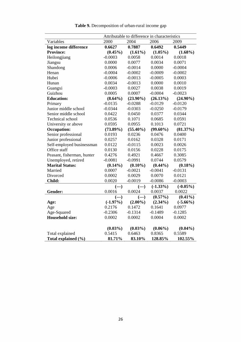
income level as the coefficients are statistically insignificant. In contrast, both variables are significant in case of rural group and show a convex effect on one’s income level. Specifically, this effect is heterogeneous across the quantiles of the income distribution that the coefficients at 5th quantile of the income distribution are much greater than those at other quantiles. For 2009, the largest gender differential can be found at two tails of the income distribution among rural and urban groups. At the 5th and 95th quantile the gap can be as large as 22%, while for the other quantiles, it drops to as low as 15%. However, such pattern cannot be consistently observed in other surveyed years. Coefficients for marital status, i.e. married and divorced, have significant and positive influence on one’s income for people under 75th percentile of the income distribution in 2009. But this effect is less obvious in other years. As for the factor of child, though the coefficients are positive, most of them are insignificant for all four reference years. In sum, we conclude that marital and child status has limited effects on one’s income. Last, household size negatively affects one’s income for both urban and rural residents at most percentiles, though the magnitude varies. 5.3 Income gap decomposition The urban-rural log income difference reported in Table 9 shows there is an increase of urban and rural income difference from 2000 to 2004. But this gap shrinks in 2006 (0.6492), and further goes down to 0.5449 in 2009. Even though our results suggest a decrease of income inequality in recent 6 years, it would be too hasty to draw the conclusion that the rural and urban income inequality has decreased in China as a whole, since our sample only covers 9 out of 31 provinces in China.

Taking a further look at the decomposition of the income gap, we find that occupation plays a dominant role in explaining the total income gap. In the year of 2006, this effect almost explains the entire income gap. Among all types of occupations, farm-activities take the lion share of the total contribution: it explains 64.5%, 62.3%, 71.8%, and 56.6% of the total urban-rural income gap. The results strongly suggest that the backwardness in rural agricultural sector is the most important factor that are causing income inequality in China. The retired groups also have a strong effect on income gap particularly in 2006 and 2009. Since urban residents usually enjoy more

welfare and more opportunities for getting reemployed after retirement than rural residents. Among all the observations, self-employed businessmen and office staffs contribute the least to the income gap.

Education is the second largest contributor of the log-income gap. Only in 2000, it has an influence under 10%, whereas for other three years, it contributes to around 25% of the income gap. We find that results for primary and junior middle school are negative, suggesting that urban-rural difference in lower level of education actually play a positive role to narrow the income gap. However, this effect has been overtaken by the effects of other educational levels. In spite of that many rural residents are able to access to compulsory education, it is not enough to compete with their counterparts in urban areas who are more open to higher level of education. As the results show that in total, education has a positive effect on forming the urban-rural income gap. The results remind us the higher level education inequality between urban and rural China becomes the primary problem that affecting the urban-rural income gap. And to address this issue, we need to consider both overall gaps in access to higher levels of education and the quality of education being assessed by urban and rural youth.

Regional location, marital status and household size have very limited power in explaining the urban-rural income gap. On the other hand, child and gender’s effects on forming the income gap are observed only in 2006 and 2009. Child has negative effects in explaining the urban-rural income inequality, suggesting that child acts as a factor that helps to narrow the inequality between two groups of residents. Age acts as a positive factor to enlarge the income gap but only in 2004 and 2006. The change in age’s effects could be a result of different factors, such as the change in the shape of the age-earnings profile, family composition, and the macroeconomic conditions of the survey years.

In total, individual’s characteristics explain most of the gap in urban-rural income. For 2000 and 2004, the unexplained income gap is up to 19.29% and 16.90%. This unexplained part is often regarded as the discrimination or due to the absence of detailed controls for all possible relevant factors of job characteristics and person-specific skills (Macpherson and Hirsch, 1995). While for 2006 and 2009, the determinants that we choose are sheer reasons for the log urban-rural income gap, and this gap would be larger if we do not consider the effects from the unexplained part. 6. Summary and Policy Suggestions Urban-rural income inequality has been a serious and persistent problem in relation with the rapid development in Chinese economy in the recent three decades. Certainly, there is a risk of oversimplification in attempting to summarize our key findings and apply it to China as a whole. After all, only 9 out of 31provinces are sampled and the core underlying data are based on household surveys about 7,000 observations in each wave. Yet the results can represent the situation of urban-rural income inequality for most parts of China — as provinces do not develop with an extreme fast speed like Shanghai or Beijing and those in west China with low economic development level and limited development potential such as Tibet and Xinjiang.

In this paper, we try take a close look at the underlying reasons behind urban-rural income inequality during the period of 2000 to 2009. An attempt has been made to identify the determinants of income level, decompose the urban-rural income gap and last to analyze the distribution of urban and rural incomes. We find that, among all the

individual characteristics, occupational type and education are the two most influential factors that determine one’s income level. People who engage in off-farm activities, especially for those who work as a senior and junior professional, have a much higher income level than those doing the farm work in both rural and urban areas. Education reflects a positive relationship with one’s income but returns for education reach the highest level in 2004 and then it decreases in 2006 and 2009. Gender income gap are evident for four years, showing males have higher income than females in China. Age exerts an inverse U-shape effect on rural residents but not so true for urban residents. Marital and child status and household size have inconsistent or unexpected effects on one’s income level.

Quantile regressions capture the non-uniform effects from individuals’ characteristics at different quantile of the income distribution. It is particularly noteworthy that for urban residents, education benefits more for the richer ones. While for the rural ones, returns from technical school and university education are prominent for the poorest. Results from both rural and urban groups show that for self-employed businessmen and peasants, the occupational returns increase along with the income distribution. Gender has greater effects on the people with lower level of income and so does the age effects on rural residents, showing that the poor are more limited by their individual characteristics.

The decomposition of the income gap indicates that occupation and education are the main contributors to the urban-rural income gap. Other effects like province location, age, marital and child status, and household size have very limited explanation power. As for the unexplained part, which sometimes refer as discrimination effects, changes before and after the year of 2005: for 2000 and 2004, results show that around 18% of income gap cannot be explained by the individual characteristics and rural residents might suffer from discrimination. While for years 2006 and 2009, there is evidence showing that several unobserved factors help narrowing the urban-rural income gap.

In regard with our findings, we provide policy suggestions that intend to narrow the current urban-rural income gap. The policy recommendations are related to investment in development infrastructures, planned urbanization process, and investment in the education system for the rural areas. It is quite common that during a rapid development process in transition and newly industrialized economies, allocation of resources is biased towards urban area. This together with low productive agricultural sector compared with service and industry sectors lead to divergence, inequality and growing inequality within and between urban/rural sectors.

First is to develop the agricultural sector in rural areas. Farm-activities in China are low in productivity due to backwardness of technology and distribution system. Family farms are usually in small scale and vulnerable to natural disasters. Government should provide more technical and financial supports to improve the productivity and crop diversification for family farms and set up of more agro-processing businesses in the towns and villages.

Second, policies should focus on the development in rural areas (Dong, 2001). This includes investment in enlarging the existed TVEs and developing for new ones locally or in cities and towns within commuting distance. As we can see, Income from non-farm activities is much higher than that from farming, exerting an equalizing influence on urban-rural income distribution. People with low income level should be offered more opportunities to get engaged in non-farm activities. However, the poorest rural

residents might not be able to afford the cost that are needed for them to seek the jobs in urban areas, while at the same time such non-farm employment opportunities are very limited in rural areas. Thus, policies that support local developments of TVE are strongly suggested to be carried out.

Above all else, the rural educational system must be transformed to provide the same opportunities for rural students as is available in urban areas. And the quality of rural schools must be upgraded to equal those of urban schools. An increasingly important issue is rural students’ access to senior high school and tertiary education. The long-standing university exam system, together with skyrocketing tuition and fees, is a higher barrier to rural students, on average, compared to urban students. If earnings are to be equalized, this differential in schooling and opportunities to getting higher education must be eliminated.

References Benjamin, D., Brandt, L., and Giles, J. (2005). The Evolution of Income Inequality in

Rural China. Economic Development and Cultural Change 53(4), 769-824. Blinder, A.S. (1973). Wage Discrimination: Reduced Form and Structural Estimates.

The Journal of Human Resources 8(4), 436-455. Constant, A., Meng, J., Tien, B. and Zimmermann, K. (2011). China’s latent human

Capital investment: Achieving Milestones and Competing for the top. IZA Discussion Paper, No. 5650.

Dong, Q.H. (2001). Structure and Strategy for In Situ rural urbanization. Urban Transformation in China. Ashgate Publishing Limited, England.

Giles, J. et al. (2012). Weathering a Storm. Survey-Based Perspectives on Employment in China in the Aftermath of the Global Financial Crisis. World Bank Policy Research Working Paper 5984.

Greenwood, J. and Jovanovic, B. (1989). Financial Development, Growth and the Distribution of Income. NBER Working Paper 3189.

Guang, L. (2010). Bring the City Back in: The Chinese Debate on Rural Problems. Harvard Contemporary China Series 16: One Country, Two Societies. Harvard Press, England.

Gustafsson, B. and Li, S. (2000). Economic Transformation and the Gender Earnings Gap in Urban China. Journal of Population Economics 13(2), 305-329.

Guo, J.X. (2005). Human Capital, the Birth Rate and the Narrowing of the Urban-Rural Income Gap. Social Science in China 3, 27-37.

Hertel, T. and Fan, Z. (2006). Labor Market Distortions, Rural-Urban Inequality and the Opening of China’s Economy, Economic Modelling 23, 76-109.

Heshmati A. (2004), “Regional Income Inequality in Selected Large Countries”, IZA Discussion Paper 2004:1307 and MTT Discussion Paper 2004:14.

Heshmati A. (2007a), “Global Trends in Income Inequality”, Hauppauge, Nova Science Publishers, NY.

Heshmati A. (2007b), “Income Inequality in China”, in Heshmati (Ed.), “Recent Developments in the Chinese Economy”, Nova Science Publishers, NY.

Hughes, J. and Maurer-Fazio, M. (2002). Effects of Marriage, Education, and Occupation on the Female/Male Wage Gap in China. Pacific Economic Review 7(1), 137-156.

Jeanneney, S.G. and Hua, P. (2008). Appreciation of the Renminbi and Urban-rural Income Inequality in China. Revue d'économie du développement 22(5), 67-92.

Johnson, D.G. (2001). The Urban-rural Disparities in China: Implications for the Future of Rural China. The University of Chicago Paper No. 01.

Kanbur, R. and Zhao, X.B. (1999). Which Regional Inequality? The Evolution of Rural-Urban and Inland-Coastal Inequality in China from 1983 to 1995. Journal of Comparative Economics 27, 686-701.

Kanbur, R. and Zhang, X.B. (2005). Fifty Years of Regional Inequality in China: A Journey through Central Planning, Reform, and Openness. Review of Development Economics, 9(1) 87-106.

Khan, A.R. and Riskin, C. (1998). Income and Inequality in China: Composition, Distribution and Growth of Household Income, 1988 to 1995. The China Quarterly 154, 221-253.

Knight, J. and Song, L. (2003). Increasing Urban Wage Inequality in China. Economics of Transition 11(4), 597-619.

Koenker, R. and Basset G. (1978). Regression quantiles. Econometrica 46(1): 1-26. Lipton, M. and Ravallion, M. (1994). Poverty and Policy. In Handbook of

Development Economics 3, Amsterdam: North-Holland. Li, S. (2009). Effects of Labor Out-Migration and Income Growth and Inequality in

Rural China. China’s Economy: Rural Reform and Agricultural Development. World Scientific Publishing, Singapore.

Li, S. and Luo, C.L. (2010). Reestimating the Income Gap between Urban and Rural Household in China. Harvard Contemporary China Series 16: One Country, Two Societies. Harvard Press, England.

Lin, Y.F., Cai, F. and Li, Z. (2002). Social Consequences of Economic Reform in China: An Analysis of Regional Disparity in the Transition Period. China and its Regions-economic Growth and Reform in Chinese Provinces, Cheltenham: Edward Elgar.

Macpherson, D. and Hirsch, B. (1995) Wages and Gender Composition: Why Do Women’s Jobs Pay Less? Journal of Labor Economics 133(3), 84-89.

Meng, X. (1998). Gender occupational segregation and its impact on the gender wage differential among rural-urban migrants: a Chinese case study. Applied Economics 30(6), 741-751.

Mincer, J. (1994). Schooling, Experience, and Earnings. Human Behavior and Social Institutions No. 2, National Bureau of Economic Research, NY.

Murphy, R. (2002). How Migrant Labor is Changing Rural China. Cambridge, UK. National Bureau of Statistics of China (2003). China Statistical Yearbook. Beijing,

China. National Bureau of Statistics (2011). China Education Yearbook. Beijing: China

Statistics Press. Oaxaca, R. (1973). Male-female Wage Differentials in Urban Labor Markets.

International Economic Review 14(3), 693-709. Putterman, L. (1992). Dualism and Reform in China. Economic Development and

Cultural Change 40(3), 467-493.

Reimers, C.W. (1983). Labor Market Discrimination against Hispanic and Black Men. The Review of Economics and Statistics 65(4), 570-579.

Sicular, T., Yue, X.M., Gustafasson, B., and Li, S. (2007). The Urban-Rural Income Gap and Inequality in China. Review of Income and Wealth 53(1), 93-126.

Wang, M.Y. and Cai, F. (2006). Gender Wage Differentials in China’s Urban Labor Marker. UNU-WIDER, Research Paper No.146.

Wei, H. and Zhao, C. (2012). Effects of International Trade on Urban-Rural Gap income in China. Finance & Trade Economics 1, 78-86.

Wei, S.J. and Yi, W. (2001). Globalization and Inequality: Evidence from within China. NBER Working Paper 8611.

World Bank (2008), World Development Indicators Database, at http://www.worldbank.org/.

Wu, X.M. and Perloff, J.M. (2005). China’s Income Distribution, 1985-2001. The Review of Economics and Statistics 87(4), 763-775.

Yang, D.T (1999). Urban-Biased Policies and Rising Income Inequality: Emerging Pattern in China’s Reforming Economy. Journal of Comparative Economics 19, 362-391.

Yang, D.T. and Zhou, H. (1999). Rural-urban disparity and sectoral labour allocation in China. Journal of Development Studies 35(3), 105-133.

Yao, S.J. Zhang, Z.Y. and Feng, G.F. (2005). Rural-Urban and Regional Inequality in Output, Income and Consumption in China under Economic Reform. Journal of Economic Studies 33(1), 4-24.

Yao, Y.J. (2005). An Empirical Analysis of Financial Development and Urban-Rural Income Gap in China. The Study of Finance and Economics 2, 5-12.

Zhang, Q., (2004). Development of Financial Intermediaries and Urban-Rural Income Inequality in China. China Journal of Finance 11, 71-79.

Table 2. Description of variables used in the Mincerian model

Variables Description lnIncome Logarithm of the total income Province: Liaoning Reference group Heilongjiang, Jiangsu,

Shandong, Henan, Hubei, Hunan, Guangxi, Guizhou

Education: Edu0 None Received no education; Reference

group Edu1 Primary Received 6 years of education Edu2 Junior middle school Received 9 years of education Edu3 Senior middle school Received 12 years of education Edu4 Technical school Received 14 or 15 years of education Edu5 University or above Received 16 or 16+ years of education Occupation: Occu1 Senior professional Doctor, professor, lawyer architect,

engineer, etc. Occu2 Junior professional Nurse, teacher, editor, photographer,

high skilled worker Occu3 Self-employed businessman Executive, Manager, government

official, businessman Occu4 Office staff Secretary, white collar, etc. Occu5 Peasant Peasant, fisherman, hunter, logger etc. Occu6 Labor, Service worker Non-technical, non-skilled worker,

waiter, doorkeeper, childcare, etc. Occu7 Retired/ Retired but working Retired/Retired but work part time or

full time Age cohort: 15-30 31-50 51-65 66 and above Age Squared: Age squared Age*age Gender: Male Reference group Female Marital Status: Single Reference group Married Divorced, widow Child: Spent time to take care of

your child last week Reference group HHsize: Household size Number of people live in the same house

20

Table 3. Percentage distribution of the variables used in the Mincerian model

2000 (all in %) 2004 (all in %) 2006 (all in %) 2009 (all in %) Characteristics Urban Rural Urban Rural Urban Rural Urban Rural Province: Liaoning 9.09 10.85 10.82 12.19 11.41 12.47 10.72 11.69 Heilongjiang 11.40 10.30 12.79 9.37 12.75 10.36 12.05 10.69 Jiangsu 13.27 13.27 14.52 12.86 14.19 12.91 14.44 12.03 Shandong 10.38 9.59 8.56 11.24 9.78 10.19 10.58 11.24 Henan 10.54 10.32 10.10 9.59 9.68 8.19 10.50 10.08 Hubei 11.67 10.88 11.73 10.62 11.31 10.66 10.98 10.65 Hunan 10.19 8.33 10.43 8.28 10.74 9.79 9.83 9.13 Guangxi 12.14 13.38 11.20 12.57 9.73 12.75 12.00 13.65 Guizhou 11.32 13.07 9.86 13.28 10.40 12.68 8.90 10.85 Education: None 12.13 22.41 11.15 20.98 10.12 25.41 9.88 23.75 Primary 12.21 26.85 11.88 28.45 9.88 22.11 9.96 23.31 Junior middle school 27.56 36.18 25.43 34.92 24.40 34.31 27.99 37.36 Senior middle school 22.40 10.86 21.01 10.84 20.90 10.99 19.80 8.89 Technical school 13.23 2.34 18.17 3.08 18.02 4.41 17.45 3.95 University or above 12.45 1.33 12.36 1.73 16.68 2.76 14.92 2.75 Occupation: Senior professional 8.12 1.26 10.38 1.45 10.31 1.81 11.11 1.56 Junior professional 20.84 7.61 16.44 5.74 17.26 7.81 14.84 8.61 Self-employed businessman 17.68 6.23 10.53 5.52 10.45 6.12 8.68 5.23 Office staff 9.17 1.98 10.34 2.42 9.83 2.34 9.17 2.50 Peasant, etc. 3.08 68.42 3.65 65.12 4.03 63.01 3.08 61.42 Labor, Service worker 16.08 10.84 12.74 8.74 12.18 12.20 15.08 13.84 Retired/ Retired but working 25.02 3.66 35.91 11.00 35.95 6.71 38.69. 7.26 Age cohort: 15-30 16.51 26.33 9.71 14.65 8.01 11.37 8.15 10.96 31-50 48.20 48.11 42.93 46.71 41.42 46.70 38.57 43.30 51-65 22.73 21.32 27.50 29.80 29.63 31.63 31.93 34.18 66 and above 14.56 5.24 19.86 8.85 20.95 10.30 21.35 11.56 Gender: Male 53.01 51.85 51.59 50.31 52.21 50.73 52.04 50.77 Female 46.99 47.15 48.41 49.69 47.79 49.27 47.96 49.23 Marital Status: Single 12.96 16.31 7.07 9.34 4.88 6.26 5.27 5.67 Married 80.17 79.42 83.55 85.41 85.95 88.41 84.06 87.97 Divorced 6.87 4.28 9.38 5.24 9.16 5.31 10.67 6.36 Child: Yes 8.82 12.23 19.23 24.66 19.13 28.70 9.74 14.80 No 81.18 87.77 80.77 75.34 80.87 71.30 90.26 85.20 Household Size: (3+) 41.96 64.87 28.85 54.54 26.85 51.32 23.88 44.61

21

Table 4. Results for OLS estimation for 2000 through 2009

*significant at 1% level; **significant at 5% level; ***significant at 10% level

2000 2004 2006 2009 Variables Urban Rural Urban Rural Urban Rural Urban Rural Constant 7.808*** 7.576*** 8.406*** 7.412*** 8.509*** 7.607*** 8.855*** 8.034*** Liaoning -- -- -- -- -- -- -- -- Heilongjiang 0.152** -0.202*** 0.021 0.317*** -0.115* 0.233*** 0.068 0.199*** Jiangsu 0.344*** 0.112** 0.353*** 0.573*** 0.111* 0.425*** 0.160*** 0.429*** Shandong 0.241*** -0.081 0.085 0.022 -0.026 0.022 0.024 0.105* Henan 0.039 -0.356*** 0.060 -0.122* 0.016 -0.139** 0.097 -0.170*** Hubei 0.043 -0.195*** -0.262*** 0.032 -0.275*** 0.121* -0.092 0.249*** Hunan 0.308*** 0.061 -0.017 -0.099 -0.124* 0.128** 0.095 0.186*** Guangxi 0.150** -0.094** -0.236*** -0.154** -0.256*** 0.001 -0.137** -0.091 Guizhou 0.114* -0.176*** 0.044 -0.084 -0.013 0.050 0.077 0.160*** Edu1 0.171*** 0.141*** 0.152** 0.195*** 0.080 0.131*** 0.111* 0.069 Edu2 0.361*** 0. 236*** 0.359*** 0.279*** 0.316*** 0.188*** 0.221*** 0.161*** Edu3 0.508*** 0.268*** 0.564*** 0.320*** 0.407*** 0.353*** 0.352*** 0.279*** Edu4 0.562*** 0.403*** 0.655*** 0.765*** 0.556*** 0.450*** 0.514*** 0.362*** Edu5 0.711*** 0.448*** 0.732*** 0.866*** 0.733*** 0.723*** 0.590*** 0.594*** Occu1 0.406*** 0.156 0.405*** 0.124 0.599*** 0.522*** 0.438*** 0.393*** Occu2 0.247*** 0.142*** 0.169*** 0.133* 0.393*** 0.302 0.252*** 0.282*** Occu3 0.238*** -0.025 -0.232*** -0.228*** 0.091 0.014*** 0.174*** 0.026 Occu4 0.286*** 0.076 0.246*** 0.149 0.318*** 0.291*** 0.278*** 0.257*** Occu5 -0.427*** -0.882*** -0.651*** -0.951*** -0.732*** -0.851*** -0.464*** -0.601*** Occu7 0.121*** -0.197*** -0.174*** -0.621*** 0.124* 0.385*** 0.126*** 0.247*** Married 0.145*** 0.040 0.019 0.209*** 0.109 0.227*** 0.311*** 0.358*** Divorced -0.024 0.041 0.004 0.136 0.095 0.272*** 0.222** 0.341*** Child -0.064 -0.051 0.021 0.050 0.105** 0.075** 0.064 -0.053 Male 0.123*** 0.148*** 0.156*** 0.227*** 0.225*** 0.273*** 0.214*** 0.240*** Age 0.019*** 0.073*** 0.005 0.061*** 0.007 0.057*** 0.005 0.047*** Age-sq -0.0002*** -0.0008*** 0.0001 -0.0006*** -0.0001 -0.0007*** -0.0001* -0.0005*** HHsize -0.024** -0.040*** -0.018 -0.055*** -0.068*** -0.044*** -0.027** -0.033** Adjusted-R2 0.2077 0.2964 0.308 0.267 0.311 0.308 0.221 0.233

22

Table 5. Result of quantile regression for urban and rural residents respectively in 2000

*significant at 1% level; **significant at 5% level; ***significant at 10% level

2000 Q5 Q25 Q50 Q75 Q95 Variables Urban Rural Urban Rural Urban Rural Urban Rural Urban Rural Constant 5.849*** 6.079*** 7.147*** 7.088*** 7.730*** 7.611*** 8.307*** 8.221*** 8.924*** 8.834*** Heilongjiang 0.335** -0.054 0.266*** -0.174*** 0.190*** -0.242*** 0.072 -0.150** -0.017 -0.006 Jiangsu 0.437*** 0.267** 0.443*** 0.195*** 0.384*** 0.149*** 0.326*** 0.215*** 0.327*** 0.069 Shandong 0.165 -0.114 0.248*** -0.075 0.315*** 0.003 0.216*** 0.087 0.421*** 0.071 Henan -0.054 -0.261** 0.126 -0.392*** 0.193*** -0.336*** 0.044 -0.223*** 0.003 -0.090 Hubei -0.022 -0.074 0.143* -0.143** 0.083 -0.185*** 0.106 -0.111** 0.199* -0.169** Hunan 0.289 0.055 0.332*** -0.090 0.326*** 0.169*** 0.200*** 0.190*** 0.087 0.087 Guangxi 0.160 0.045 0.170** -0.059 0.179*** -0.071 0.060 -0.018 0.154 -0.171** Guizhou 0.491 0.099 0.134* -0.116** 0.118** -0.177*** -0.012 -0.115** 0.193 -0.260*** Edu1 0.092 0.403*** 0.213*** 0.152*** 0.199*** 0.133*** 0.133** 0.075* 0.176** 0.041 Edu2 0.491* 0.558*** 0.391*** 0.256*** 0.351*** 0.198*** 0.295*** 0.155*** 0.315*** 0.115* Edu3 0.714** 0.544*** 0.576*** 0.281*** 0.471*** 0.216*** 0.377*** 0.196*** 0.396*** 0.056 Edu4 0.868*** 0.843*** 0.697*** 0.457*** 0.560*** 0.332*** 0.363*** 0.184*** 0.267*** 0.135 Edu5 1.039*** 0.786*** 0.831*** 0.513*** 0.696*** 0.439*** 0.532*** 0.326*** 0.442*** 0.295 Occu1 0.526** 0.174 0.308*** -0.036 0.334*** 0.141* 0.377*** 0.252*** 0.696*** 0.371 Occu2 0.441** 0.250** 0.189*** 0.058 0.196*** 0.096** 0.283*** 0.147*** 0.290** 0.388*** Occu3 0.195 -0.425*** 0.177*** -0.165*** 0.244*** -0.057 0.330*** 0.121** 0.622*** 0.443*** Occu4 0.451** 0.284** 0.238*** 0.044 0.274*** 0.075 0.298*** 0.088 0.192 0.046 Occu5 -1.374*** -1.580*** -0.972*** -1.192*** -0.277 -0.817*** -0.006 -0.515*** 0.160 -0.224*** Occu7 -0.278 -1.316*** 0.239** -0.391*** 0.196*** 0.020 0.140* 0.161** 0.036 0.198* Married 0.486*** -0.009 0.114* 0.023 0.053 0.027 0.029 0.071 -0.066 0.058 Divorced 0.165 0.188 -0.060 -0.022 -0.089 -0.019 -0.096 0.018 -0.200 0.159 Child -0.027 -0.059 -0.068 -0.047 -0.029 -0.071* -0.067 -0.042 -0.155 -0.068 Male 0.069 0.088 0.123*** 0.135*** 0.109*** 0.164*** 0.104*** 0.169*** 0.088 0.230*** Age 0.030 0.086*** 0.033*** 0.082*** 0.024*** 0.073*** 0.018** 0.051*** 0.018 0.041*** Age-sq 0.0001 -0.0009*** -0.0003*** -0.0009*** -0.0002*** -0.0008*** -0.0001** -0.0006*** -0.0002 -0.0005*** HHsize -0.001 -0.074*** -0.034** -0.039*** -0. 023** -0.031*** -0.005 -0.013 0.014*** 0.004 Pseudo R2 0.2301 0.1885 0.1529 0.2130 0.1277 0.1998 0.1014 0.1554 0.1176 0.1064

23

Table 6. Result of quantile regression for urban and rural residents respectively in 2004

*significant at 1% level; **significant at 5% level; ***significant at 10% level

2004 Q5 Q25 Q50 Q75 Q95 Variables Urban Rural Urban Rural Urban Rural Urban Rural Urban Rural Constant 7.501*** 5.057*** 8.082*** 6.514*** 8.632*** 7.703*** 8.679*** 8.363*** 9.668*** 8.951*** Heilongjiang 0.103 0.421* 0.104** 0.245*** -0.043 0.403*** -0.022 0.312*** -0.070 0.302** Jiangsu 0.344** 1.133*** 0.293*** 0.723*** 0.339*** 0.599*** 0.365*** 0.419*** 0.349*** 0.254*** Shandong 0.035 0.085 0.077 0.094 0.078 0.062 0.055 -0.069 -0.025 -0.080 Henan -0.132 -0.090 0.010 -0.121 -0.018 -0.094 0.220** -0.149** 0.434*** 0.076 Hubei -0.755** 0.277 -0.191** 0.023 -0.253*** 0.060 -0.146** -0.083 -0.165 -0.056 Hunan -0.173 -0.025 0.122** -0.066 -0.070 -0.090 -0.045 -0.030 -0.063 -0.070 Guangxi -0.734 0.168 -0.084 -0.056 -0.175** -0.077 -0.156** -0.287*** -0.163 -0.177** Guizhou 0.046 0.405** 0.094 0.006 -0.035 -0.053 0.042 -0.239*** 0.057 -0.312*** Edu1 0.267 0.340*** -0.020 0.225*** 0.139** 0.155*** 0.184** 0.138*** 0.339** 0.249*** Edu2 0.306 0.271** 0.246*** 0.256*** 0.385*** 0.245*** 0.479*** 0.261*** 0.507*** 0.359*** Edu3 0.548 0.248 0.418*** 0.421*** 0.617*** 0.291*** 0.688*** 0.307*** 0.730*** 0.374*** Edu4 0.763** 0.868*** 0.548*** 0.749*** 0.656*** 0.640*** 0.715*** 0.683*** 0.675*** 0.493*** Edu5 0.700*** 0.904*** 0.620*** 0.891*** 0.723*** 0.811*** 0.846*** 0.827*** 0.836*** 0.628*** Occu1 0.781*** 0.014 0.538*** 0.135 0.439*** 0.237* 0.228*** 0.116 0.370** 0.416 Occu2 0.157 0.267 0.326*** 0.178*** 0.228*** 0.178*** 0.044 0.186*** 0.172 0.306*** Occu3 -0.356 -0.916*** -0.355*** -0.282*** -0.254*** -0.145* -0.090 -0.018 0.249 0.388** Occu4 0.391** 0.209 0.340 0.093 0.210*** 0.224** 0.102 0.191*** 0.332** 0.366*** Occu5 -1.453*** -1.688*** -0.939*** -1.116*** -0.518*** -0.889*** -0.544*** -0.602*** -0.339 -0.256*** Occu7 -0.116 -2.048*** -0.098 -0.769*** -0.072 -0.385*** -0.144* -0.121 -0.189 0.094 Married -0.029 0.419* 0.107 0.192** 0.035 0.153*** -0.014 0.139*** 0.150 0.148 Divorced -0.055 0.385 0.045 0.216*** -0.002 0.005 0.009 0.093 0.116 0.006 Child 0.129 0.013 0.047 0.124*** -0.058 0.038 -0.028 -0.007 0.007 -0.017 Male 0.116 0.169* 0.140*** 0.242*** 0.161*** 0.198*** 0.141*** 0.186*** 0.096 0.164 Age 0.005 0.109*** 0.004 0.084*** -0.002 0.053*** 0.008 0.042*** -0.018 0.033*** Age-sq 0.0001 -0.001*** 0.0001 -0.001*** 0.0001* -0.001*** -0.0004 -0.0003*** 0.0002 -0.0003** HHsize -0.085* -0.098*** -0.045** -0.054*** -0.018 -0.049*** 0.007 -0.035*** -0.013 -0.049** Pseudo R2 0.2599 0.1669 0.2255 0.1793 0.2113 0.1838 0.1752 0.1714 0.1650 0.1290

24

Table 7. Result of quantile regression for urban and rural residents respectively in 2006

*significant at 1% level; **significant at 5% level; ***significant at 10% level

2006 Q5 Q25 Q50 Q75 Q95 variables Urban Rural Urban Rural Urban Rural Urban Rural Urban Rural Constant 7.502*** 5.974*** 8.300*** 7.073*** 8.466*** 7.839*** 8.978*** 8.674*** 9.460*** 9.550*** Heilongjiang -0.157 0.669*** 0.033 0.288*** -0.080 0.087 -0.293*** 0.081 -0.339* 0.136 Jiangsu 0.222* 0.759*** 0.145*** 0.478*** 0.119* 0.310*** -0.033 0.241*** 0.217 0.288*** Shandong -0.009 0.134 -0.017 0.120* -0.081 -0.046 -0.228** -0.055 0.559** -0.021 Henan -0.378** -0.022 0.055 -0.069 0.126* -0.253*** -0.059 -0.180** 0.185 0.060 Hubei -0.300* -0.025 -0.147** 0.193** -0.211*** 0.017 -0.387*** -0.092 -0.336** 0.392*** Hunan -0.537** 0.234 -0.093 0.222*** -0.083 0.099* -0.135 0.036 0.204 0.058 Guangxi -0.306** 0.210 -0.056 0.000 -0.056 -0.082 -0.325*** -0.166*** -0.232* -0.106 Guizhou -0.091 0.384 0.071 0.094 -0.005 -0.042 -0.120 -0.100 0.112 0.039 Edu1 -0.130 0.390*** 0.074 0.146** 0.021 0.109** 0.022 0.100** 0.077 0.271*** Edu2 -0.006 0.385*** 0.199*** 0.236*** 0.332*** 0.203*** 0.382*** 0.174*** 0.315** 0.252*** Edu3 -0.054 0.493** 0.267*** 0.410*** 0.425*** 0.341*** 0.526*** 0.300*** 0.375*** 0.301*** Edu4 0.349* 0.904*** 0.477*** 0.445*** 0.555*** 0.469*** 0.542*** 0.392*** 0.540*** 0.294*** Edu5 0.541*** 1.212*** 0.571*** 0.786*** 0.694*** 0.686*** 0.683*** 0.662*** 0.845*** 0.609*** Occu1 1.014*** 0.290 0.700*** 0.440*** 0.507*** 0.509*** 0.557*** 0.583*** 0.657*** 0.749*** Occu2 0.556** 0.429* 0.463*** 0.241*** 0.368*** 0.216*** 0.390*** 0.242*** 0.432*** 0.395*** Occu3 -0.430* -0.451* -0.161* -0.159* 0.077 0.056 0.339*** 0.168*** 0.564** 0.464*** Occu4 0.607** 0.302 0.432*** 0.130 0.300*** 0.192** 0.328*** 0.375*** 0.232 0.447*** Occu5 -2.027*** -1.794*** -1.127*** -1.140*** -0.475*** -0.760*** -0.320** -0.494*** 0.097 -0.168* Occu7 0.414* 0.214 0.183*** 0.268*** 0.068 0.364*** 0.119 0.417*** -0.088 0.372** Married 0.349 0.319 0.210** 0.176 0.144* 0.171** 0.054 0.146* 0.015 0.034 Divorced 0.433 0.363 0.228** 0.178 0.083 0.253*** -0.021 0.221** -0.116 0.033 Child 0.210** 0.046 0.103** 0.078* 0.067 0.043 0.058 0.010 0.021 0.098 Male 0.268*** 0.101 0.160*** 0.307*** 0.160*** 0.275*** 0.159*** 0.258*** 0.117** 0.282*** Age -0.002 0.059** 0.000 0.063*** 0.011* 0.055*** 0.006 0.036*** 0.005 0.021* Age-sq 0.0001 -0.0006*** 0.0000 -0.0007*** -0.0001 -0.0007*** 0.0001 -0.0005*** 0.0001 -0.0003** HHsize -0.038 -0.050 -0.060*** -0.045*** -0.079*** -0.034*** -0.061*** -0.022* -0.069 -0.048** Pseudo R2 0.3255 0.1988 0.2250 0.2271 0.2108 0.2106 0.1771 0.1670 0.1498 0.1200

25

Table 8. Result of quantile regression for urban and rural residents respectively in 2009

*significant at 1% level; **significant at 5% level; ***significant at 10% level

2009 Q5 Q25 Q50 Q75 Q95 Urban Rural Urban Rural Urban Rural Urban Rural Urban Rural Constant 7.317*** 6.126*** 8.414*** 8.036*** 8.778*** 8.401*** 9.522*** 8.803*** 10.162*** 9.086*** Heilongjiang 0.082 0.414*** 0.082 0.193*** 0.117** 0.049 -0.021 0.076 0.003 0.122 Jiangsu 0.205* 0.596*** 0.155*** 0.436*** 0.197*** 0.382*** 0.009 0.333*** 0.294** 0.287*** Shandong -0.515** 0.210 -0.088 0.062 0.018 0.084 0.034 0.047 0.234 0.008 Henan -0.029 -0.454** 0.082* -0.260** 0.192*** -0.205*** 0.120* -0.138** 0.005 0.218 Hubei -0.115 0.253 -0.057 0.199* -0.031 0.181*** -0.171** 0.195*** -0.304** 0.294*** Hunan 0.095 -0.148 0.055 0.146 0.099* 0.223*** -0.032 0.188*** 0.074 0.309*** Guangxi -0.026 -0.285 -0.074 -0.084 -0.036 -0.039 -0.281*** -0.102* -0.225* -0.015 Guizhou -0.009 0.129 0.024 0.201*** 0.144** 0.125** -0.011 0.085 0.237 0.153 Edu1 0.060 -0.017 0.050 0.053 0.109** 0.078* 0.113 0.108** 0.189 0.115 Edu2 -0.008 0.160 0.158*** 0.111* 0.245*** 0.145*** 0.306*** 0.169*** 0.284** 0.272*** Edu3 0.068 0.279 0.221*** 0.261*** 0.364*** 0.239*** 0.389*** 0.302*** 0.410*** 0.320*** Edu4 0.315** 0.612*** 0.406*** 0.312*** 0.527*** 0.307*** 0.566*** 0.421*** 0.502*** 0.328** Edu5 0.390*** 0.616** 0.491*** 0.662*** 0.612*** 0.648*** 0.619*** 0.704*** 0.588*** 0.411** Occu1 0.711*** 0.553*** 0.638*** 0.300*** 0.378*** 0.457*** 0.291*** 0.231*** 0.161 0.490* Occu2 0.519*** 0.270* 0.398*** 0.270*** 0.295*** 0.252*** 0.201*** 0.213*** 0.051 0.313*** Occu3 -0.384** -0.279 -0.109 -0.246*** 0.065 -0.065 0.282** 0.048 1.402*** 0.903*** Occu4 0.411** 0.206 0.401*** 0.070 0.359*** 0.178* 0.286*** 0.193* -0.046 0.507* Occu5 -1.115*** -1.281*** -0.789*** -0.790*** -0.558*** -0.504*** -0.251 -0.334*** 0.159 -0.165* Occu7 0.458*** 0.152 0.244*** 0.239*** 0.044 0.257*** -0.020 0.174*** -0.222 0.124 Married 0.926*** 0.873** 0.291** 0.460*** 0.192** 0.297*** 0.168** 0.200** 0.092 0.127 Divorced 0.902** 0.650* 0.211 0.390*** 0.142 0.312*** 0.121 0.213** 0.001 -0.010 Child 0.149 -0.285** 0.043 -0.120* 0.087 -0.024 0.086 0.085 0.136 0.079 Male 0.220*** 0.216** 0.193*** 0.156*** 0.157*** 0.169*** 0.192*** 0.154*** 0.218*** 0.197*** Age 0.002 0.071** -0.001 0.035*** 0.002 0.034*** -0.012 0.035*** -0.010 0.041*** Age-sq 0.0001 -0.0008** 0.0001 -0.0004*** 0.0001 -0.0004*** 0.0002*** -0.0004*** 0.0002 -0.0004*** HHsize -0.003 -0.082** -0.020 -0.049*** -0.042*** -0.030*** -0.030* -0.029*** -0.043 -0.008 Pseudo R2 0.264 0.178 0.197 0.168 0.184 0.148 0.143 0.122 0.131 0.100

26

Table 9. Decomposition of urban-rural income gap

Attributable to difference in characteristics Variables 2000 2004 2006 2009 log income difference 0.6627 0.7887 0.6492 0.5449 Province: (0.45%) (1.61%) (1.05%) (1.68%) Heilongjiang -0.0003 0.0058 0.0014 0.0018 Jiangsu 0.0000 0.0077 0.0034 0.0071 Shandong 0.0006 -0.0014 0.0000 -0.0004 Henan -0.0004 -0.0002 -0.0009 -0.0002 Hubei -0.0006 -0.0013 -0.0005 0.0003 Hunan 0.0034 -0.0013 0.0000 0.0010 Guangxi -0.0003 0.0027 0.0038 0.0019 Guizhou 0.0005 0.0007 -0.0004 -0.0023 Education: (8.64%) (23.90%) (26.13%) (24.90%) Primary -0.0135 -0.0288 -0.0129 -0.0120 Junior middle school -0.0344 -0.0303 -0.0250 -0.0179 Senior middle school 0.0422 0.0450 0.0377 0.0344 Technical school 0.0536 0.1071 0.0685 0.0591 University or above 0.0595 0.0955 0.1013 0.0721 Occupation: (73.89%) (55.40%) (99.60%) (81.37%) Senior professional 0.0193 0.0236 0.0476 0.0400 Junior professional 0.0257 0.0162 0.0328 0.0171 Self-employed businessman 0.0122 -0.0115 0.0023 0.0026 Office staff 0.0130 0.0156 0.0228 0.0175 Peasant, fisherman, hunter 0.4276 0.4921 0.4667 0.3085 Unemployed, retired -0.0081 -0.0991 0.0744 0.0579 Marital Status: (0.14%) (0.10%) (0.44%) (0.18%) Married 0.0007 -0.0021 -0.0041 -0.0131 Divorced 0.0002 0.0029 0.0070 0.0121 Child: 0.0020 -0.0019 -0.0086 -0.0003 (---) (---) (-1.33%) (-0.05%) Gender: 0.0016 0.0024 0.0037 0.0022 (---) (---) (0.57%) (0.41%) Age: (-1.97%) (2.00%) (2.34%) (-5.66%) Age 0.2176 0.1472 0.1641 0.0977 Age-Squared -0.2306 -0.1314 -0.1489 -0.1285 Household size: 0.0002

(0.03%)

0.0002

(0.03%)

0.0004

(0.06%)

0.0002

(0.04%) Total explained 0.5415 0.6463 0.8365 0.5589 Total explained (%) 81.71% 83.10% 128.85% 102.55%