Discriminative Learning with Markov Logic Networks

Tuyen N. HuynhDepartment of Computer Sciences

University of Texas at AustinAustin, TX 78712

hntuyen@cs.utexas.edu

Doctoral Dissertation Proposal

Supervising Professor: Raymond J. Mooney

Abstract

Statistical relational learning (SRL) is an emerging area of research that addresses the problem oflearning from noisy structured/relational data. Markov logic networks (MLNs), sets of weighted clauses,are a simple but powerful SRL formalism that combines the expressivity of first-order logic with theflexibility of probabilistic reasoning. Most of the existing learning algorithms for MLNs are in thegenerative setting: they try to learn a model that maximizes the likelihood of the training data. However,most of the learning problems in relational data are discriminative. So to utilize the power of MLNs, weneed discriminative learning methods that well match these discriminative tasks.

In this proposal, we present two new discriminative learning algorithms for MLNs. The first oneis a discriminative structure and weight learner for MLNs with non-recursive clauses. We use a vari-ant of ALEPH, an off-the-shelf Inductive Logic Programming (ILP) system, to learn a large set of Hornclauses from the training data, then we apply an L1-regularization weight learner to select a small set ofnon-zero weight clauses that maximizes the conditional log-likelihood (CLL) of the training data. Theexperimental results show that our proposed algorithm outperforms existing learning methods for MLNsand traditional ILP systems in term of predictive accuracy, and its performance is comparable to state-of-the-art results on some ILP benchmarks. The second algorithm we present is a max-margin weightlearner for MLNs. Instead of maximizing the CLL of the data like all existing discriminative weightlearners for MLNs, the new weight learner tries to maximize the ratio between the probability of the cor-rect label (the observable data) and and the closest incorrect label (among all the wrong labels, this onehas the highest probability), which can be formulated as an optimization problem called “1-slack” struc-tural SVM. This optimization problem can be solved by an efficient algorithm based on the cutting planemethod. However, this cutting plane algorithm requires an efficient inference method as a subroutine.Unfortunately, exact inference in MLNs is intractable. So we develop a new approximation inferencemethod for MLNs based on Linear Programming relaxation. Extensive experiments in two real-worldMLN applications demonstrate that the proposed max-margin weight learner generally achieves higherF1 scores than the current best discriminative weight learner for MLNs.

For future work, our short-term goal is to develop a more efficient inference algorithm and testour max-margin weight learner on more complex problems where there are complicated relationshipsbetween the input and output variables and among the outputs. In the longer-term, our plan is to developmore efficient learning algorithms through online learning and algorithms that revise both the clausesand their weights to improve predictive performance.

Report Documentation Page Form ApprovedOMB No. 0704-0188

Public reporting burden for the collection of information is estimated to average 1 hour per response, including the time for reviewing instructions, searching existing data sources, gathering andmaintaining the data needed, and completing and reviewing the collection of information. Send comments regarding this burden estimate or any other aspect of this collection of information,including suggestions for reducing this burden, to Washington Headquarters Services, Directorate for Information Operations and Reports, 1215 Jefferson Davis Highway, Suite 1204, ArlingtonVA 22202-4302. Respondents should be aware that notwithstanding any other provision of law, no person shall be subject to a penalty for failing to comply with a collection of information if itdoes not display a currently valid OMB control number.

1. REPORT DATE OCT 2009 2. REPORT TYPE

3. DATES COVERED 00-00-2009 to 00-00-2009

4. TITLE AND SUBTITLE Discriminative Learning with Markov Logic Networks

5a. CONTRACT NUMBER

5b. GRANT NUMBER

5c. PROGRAM ELEMENT NUMBER

6. AUTHOR(S) 5d. PROJECT NUMBER

5e. TASK NUMBER

5f. WORK UNIT NUMBER

7. PERFORMING ORGANIZATION NAME(S) AND ADDRESS(ES) University of Texas at Austin,Department of Computer Sciences,Austin,TX,78712

8. PERFORMING ORGANIZATIONREPORT NUMBER

9. SPONSORING/MONITORING AGENCY NAME(S) AND ADDRESS(ES) 10. SPONSOR/MONITOR’S ACRONYM(S)

11. SPONSOR/MONITOR’S REPORT NUMBER(S)

12. DISTRIBUTION/AVAILABILITY STATEMENT Approved for public release; distribution unlimited

13. SUPPLEMENTARY NOTES

14. ABSTRACT see report

15. SUBJECT TERMS

16. SECURITY CLASSIFICATION OF: 17. LIMITATION OF ABSTRACT Same as

Report (SAR)

18. NUMBEROF PAGES

36

19a. NAME OFRESPONSIBLE PERSON

a. REPORT unclassified

b. ABSTRACT unclassified

c. THIS PAGE unclassified

Standard Form 298 (Rev. 8-98) Prescribed by ANSI Std Z39-18

Contents

1 Introduction 3

2 Background 42.1 MLNs and Alchemy . . . . . . . . . . . . . . . . . . . . . . . . . . . . . . . . . . . . . . 42.2 ILP and Aleph . . . . . . . . . . . . . . . . . . . . . . . . . . . . . . . . . . . . . . . . . . 62.3 Structural Support Vector Machines . . . . . . . . . . . . . . . . . . . . . . . . . . . . . . 6

3 Discriminative structure and weight learning for MLNs with non-recursive clauses 93.1 Discriminative Structure Learning . . . . . . . . . . . . . . . . . . . . . . . . . . . . . . . 93.2 Discriminative Weight Learning . . . . . . . . . . . . . . . . . . . . . . . . . . . . . . . . 93.3 Experimental Evaluation . . . . . . . . . . . . . . . . . . . . . . . . . . . . . . . . . . . . 11

3.3.1 Data . . . . . . . . . . . . . . . . . . . . . . . . . . . . . . . . . . . . . . . . . . . 123.3.2 Methodology . . . . . . . . . . . . . . . . . . . . . . . . . . . . . . . . . . . . . . 123.3.3 Results and Discussion . . . . . . . . . . . . . . . . . . . . . . . . . . . . . . . . . 13

3.4 Related Work . . . . . . . . . . . . . . . . . . . . . . . . . . . . . . . . . . . . . . . . . . 153.5 Summary . . . . . . . . . . . . . . . . . . . . . . . . . . . . . . . . . . . . . . . . . . . . 16

4 Max-Margin Weight Learning for MLNs 164.1 Max-Margin Formulation . . . . . . . . . . . . . . . . . . . . . . . . . . . . . . . . . . . . 164.2 Approximate MPE inference for MLNs . . . . . . . . . . . . . . . . . . . . . . . . . . . . 174.3 Approximation algorithm for the separation oracle . . . . . . . . . . . . . . . . . . . . . . . 204.4 Experimental Evaluation . . . . . . . . . . . . . . . . . . . . . . . . . . . . . . . . . . . . 20

4.4.1 Datasets . . . . . . . . . . . . . . . . . . . . . . . . . . . . . . . . . . . . . . . . . 204.4.2 Methodology . . . . . . . . . . . . . . . . . . . . . . . . . . . . . . . . . . . . . . 214.4.3 Results and Discussion . . . . . . . . . . . . . . . . . . . . . . . . . . . . . . . . . 21

4.5 Related Work . . . . . . . . . . . . . . . . . . . . . . . . . . . . . . . . . . . . . . . . . . 244.6 Summary . . . . . . . . . . . . . . . . . . . . . . . . . . . . . . . . . . . . . . . . . . . . 25

5 Proposed Research 265.1 Improving the predictive performance . . . . . . . . . . . . . . . . . . . . . . . . . . . . . 26

5.1.1 Revising MLNs . . . . . . . . . . . . . . . . . . . . . . . . . . . . . . . . . . . . . 265.1.2 Optimizing non-linear performance metrics . . . . . . . . . . . . . . . . . . . . . . 27

5.2 More efficient learning algorithm . . . . . . . . . . . . . . . . . . . . . . . . . . . . . . . . 275.2.1 Online learning . . . . . . . . . . . . . . . . . . . . . . . . . . . . . . . . . . . . . 275.2.2 Efficient MPE and loss-augmented MPE inference algorithms . . . . . . . . . . . . 28

5.3 Experiments on additional problems . . . . . . . . . . . . . . . . . . . . . . . . . . . . . . 29

6 Conclusions 29

References 31

2

1 Introduction

A lot of data in the real world are in the form of relational/structured data such as graphs, multi-relationaldata, etc. These structured data contain a lot of entities (or objects) and relationships among the entities. Forexample, biochemical data contain information about various atoms and their interactions, social networkdata contain information about people and relationships between them, and so on. Moreover, there are alot of uncertainties in these data: uncertainty about the attributes of an objects, the type of an object, aswell as relationships between objects. Statistical relational learning (SRL) (Getoor & Taskar, 2007) whichcombines ideas from rich knowledge representations, such as first-order logic, with those from probabilisticgraphical models is an emerging area of research that addresses the problem of learning from these noisystructured/relational data.

A variety of different SRL models have been proposed over the last ten years. Among them, MarkovLogic Networks (MLNs) (Richardson & Domingos, 2006) which are sets of weighted first-order clausesare a simple but powerful formalism. It generalizes both first-order logic and Markov networks. MLNsare capable of representing all possible probability distributions over a finite number of objects (Richardson& Domingos, 2006). Moreover, MLNs also subsume other SRL representations such as probabilistic rela-tional models (Koller & Pfeffer, 1998) and relational Markov networks (Taskar, Abbeel, & Koller, 2002).Therefore, in this work, we have chosen MLNs as the model for doing research.

Most of the existing learning algorithms for MLNs are in the generative setting: they try to learn a modelthat maximizes the likelihood of the training data. However, most of the learning problems in relational dataare discriminative. For example, in the biochemical data, the goal is to learn a model that discriminatesthe active chemical compounds from the inactive ones based on their molecular structures. This problemis called the structure activity relationship prediction (SAR), and it is an important task in drug design anddiscovery (King, Sternberg, & Srinivasan, 1995). Another example is collective web-page classification.Given a set of web-pages of a department, the task is to simultaneously classify these web-pages into somepre-defined categories based on their content and the hyperlinks between them (Slattery & Craven, 1998).It is, therefore, an important research problem to develop discriminative learning algorithms for MLNs thatimproves its predictive performance on these discriminative tasks.

In this proposal, we present two new discriminative learning algorithms for MLNs. The first one isa discriminative structure and weight learner for MLNs with non-recursive clauses (Huynh & Mooney,2008). We use a variant of ALEPH (Srinivasan, 2001), an off-the-shelf Inductive Logic Programming (ILP)system, to learn a large set of Horn clauses from the training data, then we apply an L1-regularizationweight learner to select a small set of non-zero weight clauses that maximizes the conditional log-likelihood(CLL) of the training data. The experimental results show that our proposed algorithm outperforms existinglearning methods for MLNs and traditional ILP systems in term of predictive accuracy, and its performanceis comparable to state-of-the-art results on some ILP benchmarks. The second algorithm we present is amax-margin weight learner for MLNs (Huynh & Mooney, 2009). Instead of maximizing the CLL of the datalike all existing discriminative weight learners for MLNs, the new weight learner tries to maximize the ratiobetween the probability of the correct label (the observable data) and and the closest incorrect label (amongall the wrong labels, this one has the highest probability), which can be formulated as an optimizationproblem called “1-slack” structural SVM (Joachims, Finley, & Yu, 2009). Joachims et al. (2009) presentsan efficient algorithm for solving this optimization problem based on the cutting plane method. However,this cutting plane algorithm requires an efficient inference method as a subroutine. Unfortunately, exactinference in MLNs is intractable. So we develop a new approximation inference method for MLNs basedon Linear Programming relaxation. One advantage of the max-margin weight learner is that it can be

3

adapted to maximize a variety of performance metrics in addition to classification accuracy (Joachims,2005). Extensive experiments in two real-world MLN applications demonstrate that the proposed max-margin weight learner generally achieves higher F1 scores than the current best discriminative weight learnerfor MLNs.

For future work, our short-term goal is to develop a more efficient inference algorithm and test our max-margin weight learner on more complex problems where there are complicated relationships between theinput and output variables and among the outputs. In the longer-term, we plan to work on the followingproblems:

• Improving the predictive performance

All of the current discriminative weight learners assume that the structure (the clauses) is correct,and only try to fix the weights. However, it is possible that the input structure has some errors thatcannot be fixed by only modifying the weights. Hence, we plan to develop new algorithms that try torevise both the clauses and their weights at the same time. On the other hand, we also want to extendmax-margin weight learner to optimize other non-linear performance metrics.

• More efficient learning

Most of the existing learning algorithms for MLNs are in the batch setting. However, there are manycases where this approach becomes computationally expensive, especially when the number of train-ing examples are huge. One efficient alternative is online learning which processes the training ex-amples sequentially. We first plan to adapt some of the existing online max-margin weight learningalgorithms to the case of MLNs. Then we plan to look at the problem of online structure learning andrevision.

2 Background

2.1 MLNs and Alchemy

An MLN consists of a set of weighted first-order clauses. It provides a way of softening first-order logicby making situations in which not all clauses are satisfied less likely but not impossible (Richardson &Domingos, 2006). More formally, let X be the set of all propositions describing a world (i.e. the set of allground atoms), F be the set of all clauses in the MLN, wi be the weight associated with clause fi ∈ F , G fi

be the set of all possible groundings of clause fi, and Z be the normalization constant. Then the probabilityof a particular truth assignment x to the variables in X is defined as (Richardson & Domingos, 2006):

P(X = x) =1Z

exp

∑fi∈F

wi ∑g∈G fi

g(x)

=

1Z

exp

(∑

fi∈F

wini(x)

)(1)

where g(x) is 1 if g is satisfied and 0 otherwise, and ni(x) = ∑g∈G fig(x) is the number of groundings of fi

that are satisfied given the current truth assignment to the variables in X .There are two main inference tasks in MLNs. The first one is to infer the Most Probable Explanation

(MPE) or the most probable truth values for a set of unknown literals y given a set of known literals x,

4

provided as evidence (also called MAP inference). This task is formally defined as follows:

argmaxy

P(y|x) = argmaxy

1Zx

exp

(∑

iwini(x,y)

)= argmax

y ∑i

wini(x,y) (2)

where Zx is the normalization constant over all possible worlds consistent with x, and ni(x,y) is the numberof true groundings of clause fi given the truth assignment (x,y). MPE inference in MLNs is therefore equiv-alent to finding the truth assignment that maximizes the sum of the weights of satisfied clauses, a WeightedMAX-SAT problem. This is an NP-hard problem for which a number of approximate solvers exist, of whichthe most commonly used is MaxWalkSAT (Kautz, Selman, & Jiang, 1997). Recently, Riedel (2008) pro-posed a more efficient method to solve the MPE inference problem called Cutting Plane Inference (CPI),which does not require grounding the whole MLN. The CPI is a meta inference algorithm that incremen-tally constructs some parts of a large and complex Markov network and then uses some MPE inferencealgorithm to find the MPE solution on the constructed network. The main idea is that we don’t need toground the whole Markov network to find the MPE solution since there are a lot of redundant informationin the whole network. However, the CPI method only works well when the separation step returns a smallset of constraints. In the worst case, it also constructs the whole ground MLN.

The second inference task in MLNs is computing the conditional probabilities of some unknown queryliterals, y, given some evidence x. Computing these probabilities is also intractable, but there are goodapproximation algorithms such as MC-SAT (Poon & Domingos, 2006) and lifted belief propagation (Singla& Domingos, 2008).

Learning an MLN consists of two tasks: structure learning and weight learning. The weight learner canlearn weights for clauses written by a human expert or automatically induced by a structure learner. Thereare two approaches to weight learning in MLNs: generative and discriminative. In discriminative learning,we know a priori which predicates will be used to supply evidence and which ones will be queried, andthe goal is to correctly predict the latter given the former. Several discriminative weight learning methodshave been proposed, all of which try to find weights that maximize the Conditional Log Likelihood (CLL)(equivalently, minimize the negative CLL). In MLNs, the derivative of the negative CLL with respect to aweight wi is the difference of the expected number of true groundings Ew[ni] of the corresponding clausefi and the actual number according to the data ni. However, computing the expected count Ew[ni] is in-tractable. The first discriminative weight learner (Singla & Domingos, 2005) uses the structured perceptronalgorithm (Collins, 2002) where it approximates the intractable expected counts by the counts in the MPEstate computed by the MaxWalkSAT. Later, Lowd and Domingos (2007) presented a number of first-orderand second-order methods for optimizing the CLL. These methods use samples from MC-SAT to approx-imate the expected counts used to compute the gradient and Hessian of the CLL. Among them, the bestperforming is preconditioner scaled conjugate gradient (PSCG) (Lowd & Domingos, 2007). This methoduses the inverse diagonal Hessian as the preconditioner.

Regarding structure learning, there are currently two main approaches for learning clauses for MLNs.The first one is a top-down approach (Kok & Domingos, 2005; Biba, Ferilli, & Esposito, 2008). Thesealgorithms can start from an empty network or from an existing knowledge base. So they can be used forlearning a new MLN or revising an existing MLN. The algorithms usually start from the set of unit clauses,and iteratively add new clauses to the model. In each step, they try to find the best clause to add to thecurrent MLN by adding, deleting, or flipping the sign of a literal (Kok & Domingos, 2005) or performinga stochastic local search (Biba et al., 2008). The weight of each candidate clause is set to optimize the

5

weighted pseudo log-likelihood (WPLL) (Kok & Domingos, 2005) through an optimization procedure. Theneach candidate structure is scored by the WPLL (Kok & Domingos, 2005) or by the CLL (Biba et al., 2008),and the best candidate clause is add to the learnt MLN. The other approach is the bottom-up one (Mihalkova& Mooney, 2007; Kok & Domingos, 2009). Mihalkova and Mooney (2007) proposed the first bottom-upstructure learner for MLNs called BUSL. It first constructs Markov network templates from the data and thengenerates candidate clauses from these network templates. All candidate clauses are also evaluated usingWPLL, and added to the final MLN in a greedy manner. Recently, Kok and Domingos (2009) proposeda new bottom-up structure learner for MLNs called LHL. The main idea of this algorithm is based on theobservation that a relational database can be viewed as a hypergraph with constants as nodes and relations ashyperedges. Then a clause can be constructed from a path in the hypergraph. However, a hypergraph usuallycontains an exponential number of paths. So to make it tractable, the algorithm first lifts the hypergraph byjointly clustering all the constants in the relational database to form higher-level concepts, then finds pathsin the lifted hypergraph.

ALCHEMY (Kok, Singla, Richardson, & Domingos, 2005) is an open source software package forMLNs. It includes implementations for all of the major existing algorithms for structure learning, generativeweight learning, discriminative weight learning, and inference. Our proposed algorithms are implementedusing ALCHEMY.

2.2 ILP and Aleph

Traditional ILP systems discriminatively learn logical Horn-clause rules (logic programs) for inferring agiven target predicate given information provided by a set of background predicates. These purely logicaldefinitions are induced from Horn-clause background knowledge and a set of positive and negative tuples ofthe target predicate. For more information about ILP, please see (Dzeroski, 2007)

ALEPH is a popular and effective ILP system primarily based on PROGOL (Muggleton, 1995). Thebasic ALEPH algorithm consists of four steps. First, it selects a positive example to serve as the “seed”example. Then, it constructs the most specific clause, the “bottom clause”, that entails that selected example.The bottom clause is formed by conjoining all known facts about the seed example. Next, ALEPH findsgeneralizations of this bottom clause by performing a general to specific search. These generalized clausesare scored using a chosen evaluation metric, and the clause with the best score is added to the final theory.This process is repeated until it finds a set of clauses that covers all the positive examples. ALEPH allowsusers to customize each of these steps, and thereby supports a variety of specific algorithms.

2.3 Structural Support Vector Machines

In this section, we briefly review the structural SVM problem and an algorithmic schema for solving itefficiently. For more detail, see Tsochantaridis, Joachims, Hofmann, and Altun (2005), Joachims et al.(2009). In structured output prediction, we want to learn a function h : X → Y , where X is the space ofinputs and Y is the space of multivariate and structured outputs, from a set of training examples S:

S = ((x1,y1), ...,(xn,yn)) ∈ (X ×Y )n

The goal is to find a function h that has low prediction error. This can be accomplished by learning adiscriminant function f : X ×Y → R, then maximizing f over all y ∈ Y for a given input x to get theprediction.

hw(x) = argmaxy∈Y

fw(x,y)

6

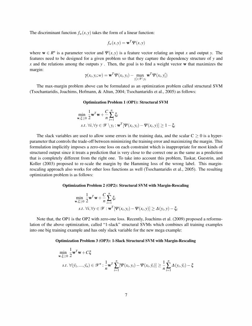
The discriminant function fw(x,y) takes the form of a linear function:

fw(x,y) = wTΨ(x,y)

where w ∈ Rn is a parameter vector and Ψ(x,y) is a feature vector relating an input x and output y. Thefeatures need to be designed for a given problem so that they capture the dependency structure of y andx and the relations among the outputs y . Then, the goal is to find a weight vector w that maximizes themargin:

γ(xi,yi;w) = wTΨ(xi,yi)− maxy′i∈Y \yi

wTΨ(xi,y′i)

The max-margin problem above can be formulated as an optimization problem called structural SVM(Tsochantaridis, Joachims, Hofmann, & Altun, 2004; Tsochantaridis et al., 2005) as follows:

Optimization Problem 1 (OP1): Structural SVM

minw,ξ≥0

12

wT w+Cn

n

∑i=1

ξi

s.t. ∀i,∀y ∈ Y \ yi : wT [Ψ(xi,yi)−Ψ(xi,y)] ≥ 1−ξi

The slack variables are used to allow some errors in the training data, and the scalar C ≥ 0 is a hyper-parameter that controls the trade-off between minimizing the training error and maximizing the margin. Thisformulation implicitly imposes a zero-one loss on each constraint which is inappropriate for most kinds ofstructured output since it treats a prediction that is very close to the correct one as the same as a predictionthat is completely different from the right one. To take into account this problem, Taskar, Guestrin, andKoller (2003) proposed to re-scale the margin by the Hamming loss of the wrong label. This margin-rescaling approach also works for other loss functions as well (Tsochantaridis et al., 2005). The resultingoptimization problem is as follows:

Optimization Problem 2 (OP2): Structural SVM with Margin-Rescaling

minw,ξ≥0

12

wT w+Cn

n

∑i=1

ξi

s.t. ∀i,∀y ∈ Y : wT [Ψ(xi,yi)−Ψ(xi,y)] ≥ ∆(yi,y)−ξi

Note that, the OP1 is the OP2 with zero-one loss. Recently, Joachims et al. (2009) proposed a reformu-lation of the above optimization, called “1-slack” structural SVMs which combines all training examplesinto one big training example and has only slack variable for the new mega example:

Optimization Problem 3 (OP3): 1-Slack Structural SVM with Margin-Rescaling

minw,ξ≥0

12

wT w+Cξ

s.t. ∀(y1, ..., yn) ∈ Y n :1n

wTn

∑i=1

[Ψ(xi,yi)−Ψ(xi, yi)] ≥1n

n

∑i=1

∆(yi, yi)−ξ

7

Algorithm 1 Cutting-plane method for solving the “1-slack structural SVMs” (Joachims et al., 2009)1: Input: S = ((x1,y1), ...,(xn,yn)),C,ε2: W ← /03: repeat4:

(w,ξ ) ← minw,ξ≥0

12

wT w+Cξ

s.t. ∀(y1, ..., yn) ∈ W :1n

wTn

∑i=1

[Ψ(xi,yi)−Ψ(xi, yi)] ≥1n

n

∑i=1

∆(yi, yi)−ξ

5: for i = 1 to n do6: yi ← argmaxy∈Y {∆(yi, y)+wTΨ(xi, y)}7: end for8: W ← W ∪{(y1, ..., yn)}9: until 1

n

n∑

i=1∆(yi, yi)− 1

n wTn∑

i=1[Ψ(xi,yi)−Ψ(xi, yi)] ≤ ξ + ε

10: return (w,ξ )

The 1-slack reformulation leads to a faster and more scalable training algorithm whose running time isprovably linear in the number of training examples (Joachims et al., 2009).

In each iteration, the algorithm 1 solves a Quadratic Programming (QP) problem (line 4) to find theoptimal weights corresponding to the current set of constraints W and a separation oracle (line 6), alsocalled a loss-augmented inference problem (Taskar, Chatalbashev, Koller, & Guestrin, 2005), to find themost violated constraint to add to W . The QP problem in line 4 can be solved by any general QP solver. Incontrast, for each representation (such as Markov networks or weighted context free grammars) a specificalgorithm is needed for solving the loss-augmented inference problem.

To enforce a sparse solution on the learned weights, we can replace the square 2-norm, wT w, on theseformulations by the 1-norm, ||w||1 = ∑n

i=1 |wi|, like previous work on 1-norm SVMs (Bradley & Man-gasarian, 1998; Zhu, Rosset, Hastie, & Tibshirani, 2003) for binary classification. Using the substitutionwi = w+

i −w−i and |wi| = w+

i +w−i with w+

i ,w−i ≥ 0 (Fung & Mangasarian, 2004), we can cast the 1-norm

minimization problem as a Linear Programming (LP) problem and use the algorithm 1 to solve the LP prob-lem by replacing the QP problem in line 4 by the transformed LP problem. A special case of the 1-normstructural SVM for the case of Markov Networks is presented in Zhu and Xing (2009).

In summary, to apply structural SVMs to a new problem, one needs to choose a representation for model,design a corresponding feature vector function Ψ(x,y), select a loss function ∆(y, y), and design algorithmsto solve the two argmax problems:

Prediction: argmaxy∈Y wTΨ(x,y)Separation Oracle: argmaxy∈Y {∆(y, y)+wTΨ(x, y)}

8

3 Discriminative structure and weight learning for MLNs with non-recursive clauses

In this section, we look at a special class of MLNs where all the clauses are non-recursive clauses whichcontain only one non-evidence literal. We present a new procedure for discriminatively learning both thestructure and parameters for this type of MLNs. The proposed approach is a two-step process. The first stepuses an off-the-shelf Inductive Logic Programming (ILP) system, ALEPH (Srinivasan, 2001), to generatea large set of potential good clauses. The second step learns the weights for these clauses, preferring toeliminate useless clauses by giving them zero weight. The weight learner in the second step tries to finda small set of non-zero weights which maximizes the conditional likelihood of the data with respect toL1-regularization. We first discuss in details the proposed approach and then the experimental evaluation.

3.1 Discriminative Structure Learning

Ideally, the search for discriminative MLN clauses would be directly guided by the goal of maximizingtheir contribution to the predictive accuracy of a complete MLN. However, this would require evaluatingevery proposed refinement to the existing set of learned clauses by relearning weights for all of the clausesand performing full probabilistic inference to determine the score of the revised model. This process iscomputationally expensive and would have to be repeated for each of the combinatorially large number ofpotential clause refinements. Evaluating clauses in standard ILP is quicker since each clause can be evaluatedin isolation based on the accuracy of its logical inferences about the target predicate. Consequently, wetake the heuristic approach of using a standard ILP method to generate clauses; however, since the logicalaccuracy of a clause is only a rough approximation of its value in a final MLN, we generate a large number ofcandidates whose accuracy is at least markedly greater than random guessing and allow subsequent weightlearning to determine their value to an overall MLN.

In order to find a set of potentially good clauses for an MLN, we use a particular configuration of ALEPH.Specifically, we use the induce cover command and m-estimate evaluation function. The induce covercommand implements a variant of PROGOL’s MDIE greedy covering algorithm (Muggleton, 1995) whichdoes not remove previously covered examples when scoring a new clause. The normal ALEPH inducecommand scores a clause based only on its coverage of currently uncovered positive examples. However,this scoring is not reflective of its use in a final MLN, and we found that the induce cover approach producesa larger set of more useful clauses that significantly increases the accuracy of our final learned MLN. Them-estimate (Dzeroski, 1991) is a Bayesian estimation of the accuracy of a clause (Cussens, 2007). The mparameter defining the underlying prior distribution is automatically set to the maximum likelihood estimateof its best value. The output of induce cover is a theory, a set of high-scoring clauses that cover all thepositive examples. However, these clauses were selected based on an m-estimate of their accuracy undera purely logical interpretation, and may not be the best ones for an MLN. Therefore, in addition to theseclauses, we also save all generated clauses whose m-estimate is greater than a predefined threshold (set to0.6 in our experiments). This provides a large set of clauses of potential utility for an MLN. We use thename ALEPH++ to refer to this version of ALEPH.

3.2 Discriminative Weight Learning

Compared to ALCHEMY’s current best discriminative weight learning method (Lowd & Domingos, 2007),our method embodies two important modifications: exact inference and L1-regularization. This sectiondescribes these two modifications.

9

First, given the restricted nature of the clauses constructed by ALEPH, we can use an efficient exactprobabilistic inference method when learning the weights instead of the approximate inference algorithmthat is used to handle the general case. Since these clauses are non-recursive definite clauses in which thetarget predicate only appears once, a grounding of any clause will contain only one grounding of the targetpredicate. For MLNs, this means that the Markov blanket of a query atom only contains evidence atoms.Consequently, the query atoms are independent given the evidence. Let Y be the set of query atoms and Xbe the set of evidence atoms, the conditional log likelihood of Y given X in this case is:

logP(Y = y|X = x) = logn

∏j=1

P(Yj = y j|X = x)

=n

∑j=1

logP(Yj = y j|X = x)

and,P(Yj = y j|X = x) =

exp(∑i∈FYjwini(x,y[Y j=y j]))

exp( ∑i∈FYj

wini(x,y[Y j=0]))+ exp( ∑i∈FYj

wini(x,y[Y j=1]))(2)

where FY j is the set of all MLN clauses with at least one grounding containing the query atom Yj,ni(x,y[Y j=y j]) is the number groundings of the ith clause that evaluate to true when all the evidence atoms inX and the query atom Yj are set to their truth values, and similarly for ni(x,y[Y j=0]) and ni(x,y[Y j=1]) when Yj

is set to 0 and 1 respectively. Then the gradient of the CLL is:

∂∂wi

logP(Y = y|X = x) =

n

∑j=1

[ni(x,y[Y j=y j])−P(Yj = 0|X = x)ni(x,y[Y j=0])

−P(Yj = 1|X = x)ni(x,y[Y j=1])]

Notice that the sum of the last two terms in the gradient is the expected count of the number of true ground-ings of the i’th formula. In general, computing this expected count requires performing approximate infer-ence under the model. For example, Singla and Domingos (Singla & Domingos, 2005) ran MPE inferenceand used the counts in the MPE state to approximate the expected counts. However, in our case, using thestandard closed world assumption for evidence predicates, all the ni’s can be computed without approximateinference since there is no ground atom whose truth value is unknown. This is a result of restricting thestructure learner to non-recursive definite clauses. In fact, this result still holds even when the clauses arenot Horn clauses. The only restriction is that the target predicates appear only once in every clause. Notethat given a set of weights, computing the conditional probability P(y|x), the CLL, and its gradient requiresonly the ni counts. So, in our case, the conditional probability P(Yj = y j|X = x), the CLL, and its gradientcan be computed exactly. In addition, these counts only need to be computed once, and ALCHEMY providesan efficient method for computing them. ALCHEMY also provides an efficient way to construct the Markovblanket of a query atom, in particular it ignores all ground formulae whose truth values are unaffected bythe value of the query atom. In our case, this helps reduce the size of the Markov blanket of a query atomsignificantly since many ground clauses are satisfied by the evidence. As a result, our exact inference is veryfast even when the MLN contains thousands of clauses.

10

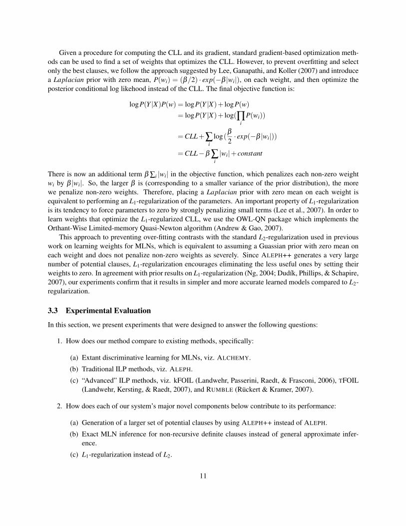
Given a procedure for computing the CLL and its gradient, standard gradient-based optimization meth-ods can be used to find a set of weights that optimizes the CLL. However, to prevent overfitting and selectonly the best clauses, we follow the approach suggested by Lee, Ganapathi, and Koller (2007) and introducea Laplacian prior with zero mean, P(wi) = (β/2) · exp(−β |wi|), on each weight, and then optimize theposterior conditional log likehood instead of the CLL. The final objective function is:

logP(Y |X)P(w) = logP(Y |X)+ logP(w)= logP(Y |X)+ log(∏

iP(wi))

= CLL+∑i

log(β2· exp(−β |wi|))

= CLL−β ∑i|wi|+ constant

There is now an additional term β ∑i |wi| in the objective function, which penalizes each non-zero weightwi by β |wi|. So, the larger β is (corresponding to a smaller variance of the prior distribution), the morewe penalize non-zero weights. Therefore, placing a Laplacian prior with zero mean on each weight isequivalent to performing an L1-regularization of the parameters. An important property of L1-regularizationis its tendency to force parameters to zero by strongly penalizing small terms (Lee et al., 2007). In order tolearn weights that optimize the L1-regularized CLL, we use the OWL-QN package which implements theOrthant-Wise Limited-memory Quasi-Newton algorithm (Andrew & Gao, 2007).

This approach to preventing over-fitting contrasts with the standard L2-regularization used in previouswork on learning weights for MLNs, which is equivalent to assuming a Guassian prior with zero mean oneach weight and does not penalize non-zero weights as severely. Since ALEPH++ generates a very largenumber of potential clauses, L1-regularization encourages eliminating the less useful ones by setting theirweights to zero. In agreement with prior results on L1-regularization (Ng, 2004; Dudık, Phillips, & Schapire,2007), our experiments confirm that it results in simpler and more accurate learned models compared to L2-regularization.

3.3 Experimental Evaluation

In this section, we present experiments that were designed to answer the following questions:

1. How does our method compare to existing methods, specifically:

(a) Extant discriminative learning for MLNs, viz. ALCHEMY.

(b) Traditional ILP methods, viz. ALEPH.

(c) “Advanced” ILP methods, viz. kFOIL (Landwehr, Passerini, Raedt, & Frasconi, 2006), TFOIL(Landwehr, Kersting, & Raedt, 2007), and RUMBLE (Ruckert & Kramer, 2007).

2. How does each of our system’s major novel components below contribute to its performance:

(a) Generation of a larger set of potential clauses by using ALEPH++ instead of ALEPH.

(b) Exact MLN inference for non-recursive definite clauses instead of general approximate infer-ence.

(c) L1-regularization instead of L2.

11

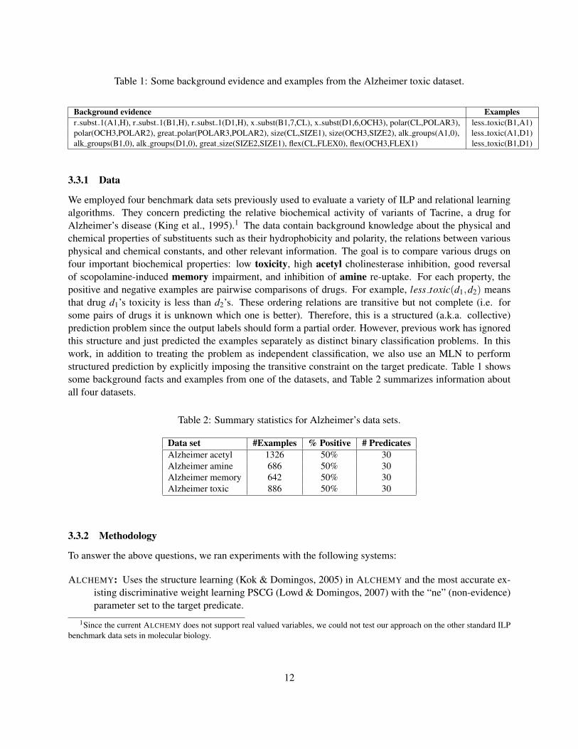
Table 1: Some background evidence and examples from the Alzheimer toxic dataset.

Background evidence Examplesr subst 1(A1,H), r subst 1(B1,H), r subst 1(D1,H), x subst(B1,7,CL), x subst(D1,6,OCH3), polar(CL,POLAR3), less toxic(B1,A1)polar(OCH3,POLAR2), great polar(POLAR3,POLAR2), size(CL,SIZE1), size(OCH3,SIZE2), alk groups(A1,0), less toxic(A1,D1)alk groups(B1,0), alk groups(D1,0), great size(SIZE2,SIZE1), flex(CL,FLEX0), flex(OCH3,FLEX1) less toxic(B1,D1)

3.3.1 Data

We employed four benchmark data sets previously used to evaluate a variety of ILP and relational learningalgorithms. They concern predicting the relative biochemical activity of variants of Tacrine, a drug forAlzheimer’s disease (King et al., 1995).1 The data contain background knowledge about the physical andchemical properties of substituents such as their hydrophobicity and polarity, the relations between variousphysical and chemical constants, and other relevant information. The goal is to compare various drugs onfour important biochemical properties: low toxicity, high acetyl cholinesterase inhibition, good reversalof scopolamine-induced memory impairment, and inhibition of amine re-uptake. For each property, thepositive and negative examples are pairwise comparisons of drugs. For example, less toxic(d1,d2) meansthat drug d1’s toxicity is less than d2’s. These ordering relations are transitive but not complete (i.e. forsome pairs of drugs it is unknown which one is better). Therefore, this is a structured (a.k.a. collective)prediction problem since the output labels should form a partial order. However, previous work has ignoredthis structure and just predicted the examples separately as distinct binary classification problems. In thiswork, in addition to treating the problem as independent classification, we also use an MLN to performstructured prediction by explicitly imposing the transitive constraint on the target predicate. Table 1 showssome background facts and examples from one of the datasets, and Table 2 summarizes information aboutall four datasets.

Table 2: Summary statistics for Alzheimer’s data sets.

Data set #Examples % Positive # PredicatesAlzheimer acetyl 1326 50% 30Alzheimer amine 686 50% 30Alzheimer memory 642 50% 30Alzheimer toxic 886 50% 30

3.3.2 Methodology

To answer the above questions, we ran experiments with the following systems:

ALCHEMY: Uses the structure learning (Kok & Domingos, 2005) in ALCHEMY and the most accurate ex-isting discriminative weight learning PSCG (Lowd & Domingos, 2007) with the “ne” (non-evidence)parameter set to the target predicate.

1Since the current ALCHEMY does not support real valued variables, we could not test our approach on the other standard ILPbenchmark data sets in molecular biology.

12

BUSL: Uses BUSL (Mihalkova & Mooney, 2007) and PSCG discriminative weight learning with the “ne”(non-evidence) parameter set to the target predicate.

ALEPH: Uses ALEPH’s standard settings with a few modifications. The maximum number of literals in anacceptable clause was set to 5. The minimum number of positive examples covered by an acceptableclause was set to 2. The upper bound on the number of negative examples covered by an acceptableclause was set to 300. The evaluation function was set to auto m, and the minimum score of anacceptable clause was set to 0.6. The induce cover command was used to learn the clauses. Wefound that this configuration gave somewhat better overall accuracy compared to those reported inprevious work.

ALEPHPSCG: Uses the discriminative weight learner PSCG to learn MLN weights for the clauses in thefinal theory returned by ALEPH. Note that PSCG also uses L2-regularization.

ALEPHExactL2 : Uses the limited-memory BFGS algorithm (Liu & Nocedal, 1989) implemented inALCHEMY to learn discriminative MLN weights for the clauses in the final theory returned by ALEPH.The objective function is CLL with L2 regularization. The CLL is computed exactly as described inSection 3.2.

ALEPH++PSCG: Like ALEPHPSCG, but learns weights for the larger set of clauses returned by ALEPH++.

ALEPH++ExactL2: Like ALEPHExactL2, but learns weights for the larger set of clauses returned byALEPH++.

ALEPH++ExactL1: Our full proposed approach using exact inference and L1-regularization to learnweights on the clauses returned by ALEPH++.

To force the predictions for the target predicate to properly constitute a partial ordering, we also triedadding to the learned MLNs a hard constraint (i.e. a clause with infinite weight) stating the transitiveproperty of the target predicate, and used the MC-SAT algorithm to perform prediction on the test data. Thisexploits the ability of MLNs to perform collective classification (structured prediction) for the complete setof test examples.

In testing, only the background facts are provided as evidence to ensure that all predictions are based onthe chemical structure of a drug. For all systems except ALEPH, a threshold of 0.5 was used to convert pre-dicted probabilities into boolean values. The predictive accuracy of these algorithms for the target predicatewere compared using 10-fold cross-validation. The significance of the results were evaluated using a two-tailed paired t-test test with a 95% confidence level. To compare the quality of the predicted probabilities,we also report the average area under the ROC curve (AUC-ROC) for all probabilistic systems by using theAUCCalculator package (Davis & Goadrich, 2006).

3.3.3 Results and Discussion

Tables 3 and 4 show the average accuracy and AUC-ROC with standard deviation for each system runningon each data set. Our complete system (ALEPH++ExactL1) achieves significantly higher accuracy thanboth ALCHEMY and BUSL on all 4 data sets and significantly higher than ALEPH on all except the memorydata set, answering questions 1(a) and 1(b). In turn, ALEPH has been shown to give higher accuracy onthese data sets than other standard ILP systems like FOIL (Landwehr et al., 2007). ALCHEMY’s existingnon-discriminative structure learners find only a few (3–5) simple clauses. Two of them are unit clauses

13

Table 3: Average predictive accuracies and standard deviations for all systems. Bold numbers indicate thebest result on a data set.

Data set ALCHEMY BUSL ALEPH ALEPH ALEPH ALEPH++ ALEPH++ ALEPH++PSCG ExactL2 PSCG ExactL2 ExactL1

Alzheimer amine 50.1 ± 0.5 51.3 ± 2.5 81.6 ± 5.1 64.6± 4.6 83.5 ± 4.7 72.0± 5.2 86.8± 4.4 89.4 ± 2.7Alzheimer toxic 54.7 ± 7.4 51.7 ± 5.3 81.7 ± 4.2 74.7± 1.9 87.5 ± 4.8 69.9± 1.2 89.5± 3.0 91.3 ± 2.8Alzheimer acetyl 48.2 ± 2.9 55.9 ± 8.7 79.6 ± 2.2 78.0± 3.2 79.5 ± 2.0 76.5± 3.7 82.1± 2.1 85.1 ± 2.4Alzheimer memory 50 ± 0.0 49.8 ± 1.6 76.0 ± 4.9 60.3± 2.1 72.6 ± 3.4 65.6± 5.4 72.9± 5.2 77.6 ± 4.9

Table 4: Average AUC-ROC and standard deviations for all systems. Bold numbers indicate the best resulton a data set.

Data set ALCHEMY BUSL ALEPH ALEPH ALEPH++ ALEPH++ ALEPH++PSCG ExactL2 PSCG ExactL2 ExactL1

Alzheimer amine .483 ± .115 .641 ± .110 .846 ± .041 .904 ± .027 .777 ± .052 .935 ± .032 .954 ± .019Alzheimer toxic .622 ± .079 .511 ± .079 .904 ± .034 .930 ± .035 .874 ± .041 .937 ± .029 .939 ± .035Alzheimer acetyl .473 ± .037 .588 ± .108 .850 ± .018 .850 ± .020 .810 ± .040 .899 ± .015 .916 ± .013Alzheimer memory .452± .088 .426 ± .065 .744 ± .040 .768 ± .032 .737 ± .059 .813 ± .059 .844 ± .052

for the target predicate, such as great ne(a1,a1) and great ne(a1,a2); the others capture the transitive natureof the target relation. Therefore, even after they are discriminatively weighted, their predictions are notsignificantly better than random guessing.

The ablations that remove components from our overall system demonstrate the important contri-bution of each component. Regarding question 2(b), the systems using general approximate inference(ALEPHPSCG and ALEPH++PSCG) perform much worse than the corresponding versions that use ex-act inference (ALEPHExactL2 and ALEPH++ExactL2). Therefore, when there is a target predicate thatcan be accurately inferred using non-recursive definite clauses, exploiting this restriction to perform exactinference is a clear win.

Regarding question 2(a), ALEPH++ExactL2 performs significantly better than ALEPHExactL2, demon-strating the advantage of learning a large set of potential clauses and combining them with learned weightsin an overall MLN. Across the four datasets, ALEPH++ returns an average of 6,070 clauses compared toonly 10 for ALEPH.

Table 5 presents average accuracies with standard deviations for the MLN systems when we includea transitivity clause for the target predicate. This constraint improves the accuracies of ALEPHExactL2,ALEPH++ExactL2, and ALEPH++ExactL1, but sometimes decreases the accuracy of other systems, suchas ALEPHPSCG. This can be explained as follows. Since most of the predictions of ALEPH++ExactL1 arecorrect, enforcing transitivity can correct some of the wrong ones. However, ALEPHPSCG produces manywrong predictions, so forcing them to obey transitivity can produce additional incorrect predictions.

Regarding question 2(c), using L1-regularization gives significantly higher accuracy and AUC-ROC thanusing standard L2-regularization. This comparison was only performed for ALEPH++ since this is when theweight-learner must choose from a large set of candidate clauses by encouraging zero weights. Table 6compares the average number of clauses learned (after zero-weight clauses are removed) for L1 and L2

14

Table 5: Average predictive accuracies and standard deviations for MLN systems with transitive clauseadded.

Data set ALCHEMY BUSL ALEPH ALEPH ALEPH++ ALEPH++ ALEPH++PSCG ExactL2 PSCG ExactL2 ExactL1

Alzheimer amine 50.0 ± 0.0 52.2 ± 5.3 61.4 ± 3.6 87.0 ± 3.3 72.9± 3.5 91.7± 3.5 90.5 ± 3.6Alzheimer toxic 50.0 ± 0.0 50.1 ± 0.8 73.3 ± 1.8 88.8 ± 4.8 68.4± 1.5 91.4± 3.6 91.9 ± 4.1Alzheimer acetyl 53.0 ± 6.2 54.1 ± 4.9 80.4 ± 2.7 84.1 ± 3.1 83.3± 2.5 88.7± 2.1 87.6 ± 2.7Alzheimer memory 50.0 ± 0.0 50.1 ± 0.5 58.9 ± 2.3 76.5 ± 3.5 70.1± 5.2 81.3± 4.8 81.3 ± 4.1

Table 6: Average number of clauses learned

Data set ALEPH++ ALEPH++ ALEPH++ExactL2 ExactL1

Alzheimer amine 7061 5070 3477Alzheimer toxic 2034 1194 747Alzheimer acetyl 8662 5427 2433Alzheimer memory 6524 4250 2471

regularization. As expected, the final learned MLNs are much simpler when using L1-regularization. Onaverage, L1-regularization reduces the size of the final set of clauses by 26% compared to L2-regularization.

Regarding question 1(c), several researchers have tested “advanced” ILP systems on our datasets. Ta-ble 7 compares our best results to those reported for TFOIL (a combination of FOIL and tree augmentednaive Bayes), kFOIL (a kernelized version of FOIL), and RUMBLE (a max-margin approach to learning aweighted rule set). Our results are competitive with these recent systems. Additionally, unlike MLNs, thesemethods do not create “declarative” theories that have a well-defined possible worlds semantics.

3.4 Related Work

Using an off-the-shelf ILP system to learn clauses for MLNs is not a new idea. Richardson and Domingos(2006) used CLAUDIEN, an non-discriminative ILP system that can learn arbitrary first-order clauses, tolearn MLN structure and to refine the clauses from a knowledge base. Kok and Domingos (2005) reportedexperimental results comparing their MLN structure learner to learning clauses using CLAUDIEN, FOIL,and ALEPH. However, since this previous work used the relatively small set of clauses produced by theseunaltered ILP systems, the performance was not very good. ILP systems have also been used to learnstructures for other SRL models. The SAYU system (Davis, Burnside, de Castro Dutra, Page, & Costa,2005) used ALEPH to propose candidate features for a Bayesian network classifier. Muggleton(Muggleton,2000) used PROGOL, another popular ILP system, to learn clauses for Stochastic Logic Programs (SLPs).

When restricted to learning non-recursive clauses for classification, our approach is equivalent to usingALEPH to construct features for use by L1-regularized logistic regression. Under this view, our approach isclosely related to MACCENT (Dehaspe, 1997), which uses a greedy approach to induce clausal constraintsthat are used as features for maximum-entropy classification. One difference between our approach andMACCENT is that we use a two-step process instead of greedily adding one feature at a time. In addition, ourclauses are induced in a bottom-up manner while MACCENT uses top-down search; and our weight learner

15

Table 7: Average predictive accuracies and standard deviations of our best results and other “advanced” ILPsystems.

Data set Our best results TFOIL kFOIL RUMBLE

Alzheimer amine 91.7± 3.5 87.5 ± 4.4 88.8 ± 5.0 91.1Alzheimer toxic 91.9 ± 4.1 92.1 ± 2.6 89.3 ± 3.5 91.2Alzheimer acetyl 88.7± 2.1 82.8 ± 3.8 87.8 ± 4.2 88.4Alzheimer memory 81.3 ± 4.1 80.4 ± 5.3 80.2 ± 4.0 83.2

employs L1-regularization which makes it less prone to overfitting. Unfortunately, we could not compareexperimentally to MACCENT since “only an implementation of a propositional version of MACCENT isavailable, which only handles data in attribute-value (vector) format” (Landwehr et al., 2007). Additionally,MLNs are a more expressive formalism that also allows for structured prediction, as demonstrated by ourresults that include a transitivity constraint on the target relation.

3.5 Summary

We have found that existing methods for learning Markov Logic Networks perform very poorly when testedon several benchmark ILP problems in drug design. We have presented a new approach to constructingMLNs that discriminatively learns both their structure and parameters to optimize predictive accuracy fora stated target predicate when given evidence specified with a defined set of background predicates. Ituses a variant of an existing ILP system (ALEPH) to construct a large number of potential clauses and theneffectively learns their parameters by altering existing discriminative MLN weight-learning methods to uti-lize exact inference and L1 regularization. Experimental results show that the resulting system outperformsexisting MLN and ILP methods and gives state-of-the-art results for the Alzheimer’s-drug benchmarks.

4 Max-Margin Weight Learning for MLNs

In Section 3, we aim to learn a model that maximizes the CLL of the data. If the goal is to predict accuratetarget-predicate probabilities, that approach is well motivated. However, in many applications, the actualgoal is to maximize an alternative performance metric such as classification accuracy or F-measure. Max-margin methods are a competing approach to discriminative training that are well-founded in computationallearning theory and have demonstrated empirical success in many applications (Cristianini & Shawe-Taylor,2000). They also have the advantage that they can be adapted to maximize a variety of performance metricsin addition to classification accuracy (Joachims, 2005). In this section, we present a max-margin approachto weight learning in MLNs based on the general framework for max-margin training of structured models(Tsochantaridis et al., 2005; Joachims et al., 2009).

4.1 Max-Margin Formulation

All of the current discriminative weight learners for MLNs try to find a weight vector w that optimizesthe conditional log-likelihood P(y|x) of the query atoms y given the evidence x. However, an alternativeapproach is to learn a weight vector w that maximizes the ratio:

P(y|x,w)P(y|x,w)

16

between the probability of the correct truth assignment y and the closest competing incorrect truth assign-ment y = argmaxy∈Y\y P(y|x). Applying equation 1 and taking the log, this problem translates to maximiz-ing the margin:

γ(x,y;w) = wT n(x,y)−wT n(x, y)

= wT n(x,y)− maxy∈Y\y

wT n(x, y)

Note that, this translation holds for all log-linear models. For example, if we apply it to a CRF (Lafferty,McCallum, & Pereira, 2001) then the result model is an M3N (Taskar et al., 2003). In fact, this translationis the connection between log-linear models and linear classifiers (Collins, 2004).

In turn, the max-margin problem above can be formulated as a “1-slack” structural SVM as described insection 2.3:

Optimization Problem 4 (OP4): Max-Margin Markov Logic Networks

minw,ξ≥0

12

wT w+Cξ

s.t. ∀y ∈ Y : wT [n(x,y)−n(x, y)] ≥ ∆(y, y)−ξ

So for MLNs, the number of true groundings of the clauses n(x,y) plays the role of the feature vectorfunction Ψ(x,y) in the general structural SVM problem. In other words, each clause in an MLN can beviewed as a feature representing a dependency between a subset of inputs and outputs or a relation amongseveral outputs.

As mentioned, in order to apply Algorithm 1 to MLNs, we need algorithms for solving the followingtwo problems:

Prediction: argmaxy∈Y wT n(x,y)Separation Oracle: argmaxy∈Y{∆(y, y)+wT n(x, y)}

The prediction problem is just the (intractable) MPE inference problem discussed in section 2.1. We can useMaxWalkSAT to get an approximate solution, but we have found that models trained with MaxWalkSAThave very low predictive accuracy. On the other hand, recent work (Finley & Joachims, 2008) has found thatfully-connected pairwise Markov random fields, a special class of structural SVMs, trained with overgener-ating approximate inference methods (such as relaxation) preserves the theoretical guarantees of structuralSVMs trained with exact inference, and exhibits good empirical performance. Based on this result, wesought a relaxation-based approximation for MPE inference. We first present an LP-relaxation algorithmfor MPE inference, then show how to modify it to solve the separation oracle problem for some specific lossfunctions.

4.2 Approximate MPE inference for MLNs

MPE inference in MLNs is a special case of MAP inference in Markov networks with binary variables,and there has been a lot of work on approximation algorithms for solving MAP inference using convexrelaxation, see (Kumar, Kolmogorov, & Torr, 2009) for more details. However, these methods are notsuitable for MLNs. First, most of them are for Markov networks with unary and pairwise potential functionswhile a ground MLN may contain many high-order cliques. The algorithms can be extended to handle high-order potential functions (Werner, 2008), but they become computationally expensive. Second, they do nothandle deterministic factor, i.e. infinite potential function. On the other hand, MPE inference in MLNs is

17

equivalent to the Weighted MAX-SAT problem, and there are also significant work on approximating thisNP-hard problem using LP-relaxation (Asano & Williamson, 2002; Asano, 2006). The existing algorithmsfirst relax and convert the Weighted MAX-SAT problem into a linear or semidefinite programming problem,then solve it and apply a randomized rounding method to obtain an approximate integral solution. Thesemethods cannot be directly applied to MLNs, since they require the weights to be positive while MLNweights can be negative or infinite. However, we can modify the conversion used in these approaches tohandle the case of negative and infinite weights.

Based on the evidence and the closed world assumption, a ground MLN contains only ground clausesof the unknown ground atoms after removing all trivially satisfied and unsatisfied clauses. The follow-ing procedure translates the MPE inference in a ground MLN into an Integer Linear Programming (ILP)problem.

1. Assign a binary variable yi to each unknown ground atom. yi is 1 if the corresponding ground atom isT RUE and 0 if the ground atom is FALSE.

2. For each ground clause C j with infinite weight, add the following linear constraint to the ILP problem:

∑i∈I+

j

yi + ∑i∈I−j

(1− yi) ≥ 1

where I+j , I−j are the sets of positive and negative ground literals in clause C j respectively.

3. For each ground clause C j with positive weight w j, introduce a new auxiliary binary variable z j, addthe term w jz j to the objective function, and add the following linear constraint to the ILP problem:

∑i∈I+

j

yi + ∑i∈I−j

(1− yi) ≥ z j

z j is 1 if the corresponding ground clause is satisfied.

4. For each ground clause C j with k ground literals and negative weight w j, introduce a new auxiliaryboolean variable z j, add the term −w jz j to the objective function and add the following k linearconstrains to the ILP problem:

1− yi ≥ z j, i ∈ I+j

yi ≥ z j, i ∈ I−j

The final ILP has the following form:Optimization Problem 5 (OP5):

maxyi,zi

∑C j∈C+

w jz j + ∑C j∈C−

−w jz j

s.t. ∑i∈I+

j

yi + ∑i∈I−j

(1− yi) ≥ 1 ∀ C j where w j = ∞

∑i∈I+

j

yi + ∑i∈I−j

(1− yi) ≥ z j ∀C j ∈C+

1− yi ≥ z j ∀ i ∈ I+j and C j ∈C−

yi ≥ z j ∀ i ∈ I−j and C j ∈C−

yi,z j ∈ {0,1}

18

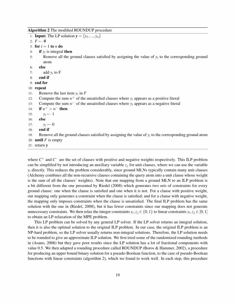
Algorithm 2 The modified ROUNDUP procedure1: Input: The LP solution y = {y1, ...,yn}2: F ← /03: for i = 1 to n do4: if yi is integral then5: Remove all the ground clauses satisfied by assigning the value of yi to the corresponding ground

atom6: else7: add yi to F8: end if9: end for

10: repeat11: Remove the last item yi in F12: Compute the sum w+ of the unsatisfied clauses where yi appears as a positive literal13: Compute the sum w− of the unsatisfied clauses where yi appears as a negative literal14: if w+ > w− then15: yi ← 116: else17: yi ← 018: end if19: Remove all the ground clauses satisfied by assigning the value of yi to the corresponding ground atom20: until F is empty21: return y

where C+ and C− are the set of clauses with positive and negative weights respectively. This ILP problemcan be simplified by not introducing an auxiliary variable z j for unit clauses, where we can use the variableyi directly. This reduces the problem considerably, since ground MLNs typically contain many unit clauses(Alchemy combines all the non-recursive clauses containing the query atom into a unit clause whose weightis the sum of all the clauses’ weights). Note that our mapping from a ground MLN to an ILP problem isa bit different from the one presented by Riedel (2008) which generates two sets of constraints for everyground clause: one when the clause is satisfied and one when it is not. For a clause with positive weight,our mapping only generates a constraint when the clause is satisfied; and for a clause with negative weight,the mapping only imposes constraints when the clause is unsatisfied. The final ILP problem has the samesolution with the one in (Riedel, 2008), but it has fewer constraints since our mapping does not generateunnecessary constraints. We then relax the integer constraints yi,z j ∈ {0,1} to linear constraints yi,z j ∈ [0,1]to obtain an LP-relaxation of the MPE problem.

This LP problem can be solved by any general LP solver. If the LP solver returns an integral solution,then it is also the optimal solution to the original ILP problem. In our case, the original ILP problem is anNP-hard problem, so the LP solver usually returns non-integral solutions. Therefore, the LP solution needsto be rounded to give an approximate ILP solution. We first tried some of the randomized rounding methodsin (Asano, 2006) but they gave poor results since the LP solution has a lot of fractional components withvalue 0.5. We then adapted a rounding procedure called ROUNDUP (Boros & Hammer, 2002), a procedurefor producing an upper bound binary solution for a pseudo-Boolean function, to the case of pseudo-Booleanfunctions with linear constraints (algorithm 2), which we found to work well. In each step, this procedure

19

picks one fractional component and rounds it to 1 or 0. Hence, this process terminates in at most n steps,where n is the number of query atoms. Note that due to the dependencies between the variables yi’s andz j’s (the linear constraints of the LP problem), this modified ROUNDUP procedure does not guarantee animprovement in the value of the objective function in each step like the original ROUNDUP procedurewhere all the variables are independent.

4.3 Approximation algorithm for the separation oracle

The separation oracle adds an additional term, the loss term, to the objective function. So, if we can representthe loss as a linear function of the yi variables of the LP-relaxation, then we can use the above approximationalgorithm to also approximate the separation oracle. In this work, we consider two loss functions. The firstone is the 0/1 loss function, ∆0/1(yT,y) where yT is the true assignment and y is some predicted assignment.For this loss function, the separation oracle is the same as the MPE inference problem since the loss functiononly adds a constant 1 to the objective function. Hence, in this case, to find the most violated constraint,we can use the LP-relaxation algorithm above or any other MPE inference algorithm. This 0/1 loss makesthe separation oracle problem easier but it does not scale the margin by how different yT and y are. It onlyrequires a unit margin for all assignments y different from the true assignment yT. To take into account thisproblem, we consider the second loss function that is the number of misclassified atoms or the Hammingloss:

∆Hamming(yT,y) =n

∑i[yT

i = yi]

=n

∑i[(yT

i = 0∧ yi = 1)∨ (yTi = 1∧ yi = 0)]

From the definition, this loss can be represented as a function of the yi’s:

∆Hamming(yT,y) = ∑i:yT

i =0

yi + ∑i:yT

i =1

(1− yi)

which is equivalent to adding 1 to the coefficient of yi if the true value of yi is 0 and subtracting 1 from thecoefficient of yi if the true value of yi is 1. So we can use the LP-relaxation algorithm above to approximatethe separation oracle with this Hamming loss function. Another possible loss function is the F1 loss which isequivalent to 1-F1. Unfortunately, this loss is a non-linear function, so we cannot use the above approach tooptimize it. Developing algorithms for optimizing or approximating this loss function is an area for futurework.

4.4 Experimental Evaluation

This section presents experiments comparing the max-margin weight learner to the weight learners in section3 and the PSCG algorithm.

4.4.1 Datasets

Besides those Alzheimer’s datasets described in section 3.3.1, we also ran experiments on two other large,real-world datasets: WebKB for collective web-page classification, and CiteSeer for bibliographic citationsegmentation.

20

The WebKB dataset (Slattery & Craven, 1998) consists of labeled web pages from the computer sciencedepartments of four universities. Different versions of this data have been used in previous work. To make afair comparison, we used the version from (Lowd & Domingos, 2007), which contains 4,165 web pages and10,935 web links. Each page is labeled with a subset of the categories: course, department, faculty, person,professor, research project, and student. The goal is to predict these categories from the words and links onthe web pages. We used the same simple MLN from (Lowd & Domingos, 2007), which only has clausesrelating words to page classes, and page classes to the classes of linked pages.

Has(+word, page) => PageClass(+class, page)!Has(+word, page) => PageClass(+class, page)PageClass(+c1, p1)∧Linked(p1, p2) => PageClass(+c2, p2)

The plus notation creates a separate clause for each pair of word and page class, and for each pair of classes.The final MLN consists of 10,891 clauses, and a weight must be learned for each one. After grounding, eachdepartment results in an MLN with more than 100,000 ground clauses and 5,000 query atoms in a complexnetwork. This also results in a large LP-relaxation problem for MPE inference.

For CiteSeer , we used the dataset and MLN used in (Poon & Domingos, 2007). The dataset has 1,563citations and each of them is segmented into three fields: Author, Title and Venue. The dataset has fourdisconnected segments corresponding to four different research topics. We used the simplest MLN in (Poon& Domingos, 2007), which is the isolated segmentation model. Despite its simplicity, after grounding, thismodel results in a large network with more than 30,000 query atoms and 110,000 ground clauses.

All the datasets and MLNs can be found at the Alchemy website.2

4.4.2 Methodology

For the max-margin weight learner, we used a simple process for selecting the value of the C parameter. Foreach train/test split, we trained the algorithm with five different values of C: 1, 10, 100, 1000, and 10000,then selected the one which gave the highest average F1 score on training. The ε parameter was set to 0.001.To solve the QP problems in Algorithm 1 and LP problems in the LP-relaxation MPE inference, we usedthe MOSEK 3 solver. The PSCG algorithm was carefully tuned by its author. For MC-SAT, we used thedefault setting, 100 burn-in and 1000 sampling iterations, and predict that an atom is true iff its probabilityis at least 0.5.

For the Alzheimer’s datasets, we used the same experimental setup mentioned in section 3.3.2, and ranfour-fold cross-validation (i.e. leave one university/topic out) on the WebKB and CiteSeer datasets.

We used F1, the harmonic mean of recall and precision, to measure the performance of each algorithm onthe WebKB and CiteSeer datasets. This is the standard evaluation metric in multi-class text categorizationand information extraction.

4.4.3 Results and Discussion

Table 8 and 10 present the performance of different systems on the WebKB and Citeseer datasets. Eachsystem is named by the weight learner used, the loss function used in training, and the inference algorithmused in testing. For max-margin (MM) learner with margin rescaling, the inference used in training is theloss-augmented version of the one used in testing. For example, MM-∆Hamming-LPRelax is the max-margin

2http://alchemy.cs.washington.edu3http://www.mosek.com/

21

Table 8: F1 scores on WebKB

Cornell Texas Washington Wisconsin AveragePSCG-MCSAT 0.418 0.298 0.577 0.568 0.465PSCG-LPRelax 0.420 0.310 0.588 0.575 0.474MM-∆0/1-MaxWalkSAT 0.150 0.162 0.122 0.122 0.139MM-∆0/1-LPRelax 0.282 0.372 0.675 0.521 0.462MM-∆Hamming-LPRelax 0.580 0.451 0.715 0.659 0.601

Table 9: F1 scores of different inference algorithms on WebKB

Cornell Texas Washington Wisconsin AveragePSCG-MCSAT 0.418 0.298 0.577 0.568 0.465PSCG-MaxWalkSAT 0.161 0.140 0.119 0.129 0.137PSCG-LPRelax 0.420 0.310 0.588 0.575 0.474MM-∆Hamming-MCSAT 0.470 0.370 0.573 0.481 0.473MM-∆Hamming-MaxWalkSAT 0.185 0.184 0.150 0.154 0.168MM-∆Hamming-LPRelax 0.580 0.451 0.715 0.659 0.601

weight learner using the loss-augmented (Hamming loss) LP-relaxation MPE inference algorithm in trainingand the LP-relaxation MPE inference algorithm in testing.

Table 8 shows that the model trained using MaxWalkSAT has very low predictive accuracy. This resultis consistent with the result presented in (Riedel, 2008) which also found that the MPE solution found byMaxWalkSAT is not very accurate. Using the proposed LP-relaxation MPE inference improves the F1 scorefrom 0.139 to 0.462, the MM-∆0/1-LPRelax system. Then the best system is obtained by rescaling themargin and training with our loss-augmented LP-relaxation MPE inference, which is the only differencebetween MM-∆Hamming-LPRelax and MM-∆0/1-LPRelax. The MM-∆Hamming-LPRelax achieves the best F1score (0.601), which is much higher than the 0.465 F1 score obtained by the current best discriminativeweight learner for MLNs, PSCG-MCSAT.

Table 9 compares the performance of the proposed LP-relaxation MPE inference algorithm against MC-SAT and MaxWalkSAT on the best trained models by PSCG and MM on the WebKB dataset. In both cases,the LP-relaxation MPE inference achieves much better F1 scores than those of MCSAT and MaxWalkSAT.This demonstrates that the approximate MPE solution found by the LP-relaxation algorithm is much moreaccurate than the one found by the MaxWalkSAT algorithm. The fact that the performance of the LP-relaxation is higher than that of MCSAT shows that in collective classification it is better to use the MPEsolution as the prediction than the marginal prediction.

For the WebKB dataset, there are other results reported in previous work, such as those in (Taskar et al.,2003), but those results cannot be directly compared to our results since we use a different version of thedataset and test on a more complicated task (a page can have multiple labels not just one).

On the Citeseer results presented in Table 10, the performance of max-margin methods are very closeto those of PSCG. However, its performance is much more stable. Table 11 shows the performance of MMweight learners and PSCG with different parameter values by varying the C value for MM and the numberof iterations for PSCG. The best number of iterations for PSCG is 9 or 10. In principle, we should run PSCGuntil it converges to get the optimal weight vector. However, in this case, the performance of PSCG drops

22

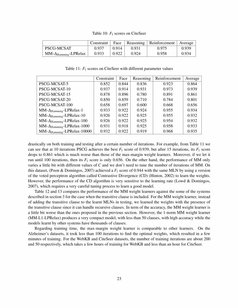
Table 10: F1 scores on CiteSeer

Constraint Face Reasoning Reinforcement AveragePSCG-MCSAT 0.937 0.914 0.931 0.975 0.939MM-∆Hamming-LPRelax 0.933 0.922 0.924 0.958 0.934

Table 11: F1 scores on CiteSeer with different parameter values

Constraint Face Reasoning Reinforcement AveragePSCG-MCSAT-5 0.852 0.844 0.836 0.923 0.864PSCG-MCSAT-10 0.937 0.914 0.931 0.973 0.939PSCG-MCSAT-15 0.878 0.896 0.780 0.891 0.861PSCG-MCSAT-20 0.850 0.859 0.710 0.784 0.801PSCG-MCSAT-100 0.658 0.697 0.600 0.668 0.656MM-∆Hamming-LPRelax-1 0.933 0.922 0.924 0.955 0.934MM-∆Hamming-LPRelax-10 0.926 0.922 0.925 0.955 0.932MM-∆Hamming-LPRelax-100 0.926 0.922 0.925 0.954 0.932MM-∆Hamming-LPRelax-1000 0.931 0.918 0.925 0.958 0.933MM-∆Hamming-LPRelax-10000 0.932 0.922 0.919 0.968 0.935

drastically on both training and testing after a certain number of iterations. For example, from Table 11 wecan see that at 10 iterations PSCG achieves the best F1 score of 0.939, but after 15 iterations, its F1 scoredrops to 0.861 which is much worse than those of the max-margin weight learners. Moreover, if we let itrun until 100 iterations, then its F1 score is only 0.656. On the other hand, the performance of MM onlyvaries a little bit with different values of C and we don’t need to tune the number of iterations of MM. Onthis dataset, (Poon & Domingos, 2007) achieved a F1 score of 0.944 with the same MLN by using a versionof the voted perceptron algorithm called Contrastive Divergence (CD) (Hinton, 2002) to learn the weights.However, the performance of the CD algorithm is very sensitive to the learning rate (Lowd & Domingos,2007), which requires a very careful tuning process to learn a good model.

Table 12 and 13 compares the performance of the MM weight learners against the some of the systemsdescribed in section 3 for the case when the transitive clause is included. For the MM weight learner, insteadof adding the transitive clause to the learnt MLNs in testing, we learned the weights with the presence ofthe transitive clause since it can handle recursive clauses. In term of the accuracy, the MM weight learner isa little bit worse than the ones proposed in the previous section. However, the 1-norm MM weight learner(MM-L1-LPRelax) produces a very compact model, with less than 50 clauses, with high accuracy while themodels learnt by other systems have thousands of clauses.

Regarding training time, the max-margin weight learner is comparable to other learners. On theAlzheimer’s datasets, it took less than 100 iterations to find the optimal weights, which resulted in a fewminutes of training. For the WebKB and CiteSeer datasets, the number of training iterations are about 200and 50 respectively, which takes a few hours of training for WebKB and less than an hour for CiteSeer.

23

Table 12: Average predictive accuracies and standard deviations on Alzheimer’s datasets with transitiveclause added

Data set ALEPH ALEPH++ ALEPH++ ALEPH ALEPH++ ALEPH++ExactL2 ExactL2 ExactL1 MM-LPRelax MM-LPRelax MM-L1-LPRelax

Alzheimer amine 87.0 ± 3.3 91.7± 3.5 90.5 ± 3.6 87.0 ± 2.2 89.2± 2.9 88.8 ± 3.0Alzheimer toxic 88.8 ± 4.8 91.4± 3.6 91.9 ± 4.1 88.5 ± 4.2 90.8± 3.6 91.6 ± 4.3Alzheimer acetyl 84.1 ± 3.1 88.7± 2.1 87.6 ± 2.7 86.3 ± 2.8 88.3± 2.9 87.9 ± 2.8Alzheimer memory 76.5 ± 3.5 81.3± 4.8 81.3 ± 4.1 79.1 ± 3.0 81.5± 4.2 80.7 ± 4.0

Table 13: Average number of clauses learned on Alzheimer’s datasets

Data set ALEPH ALEPH++ ALEPH++ ALEPH++ ALEPH++ ALEPH++ExactL2 ExactL1 MM-LPRelax MM-L1-LPRelax

Alzheimer amine 10 7061 5070 3477 6981 35Alzheimer toxic 9 2034 1194 747 2034 25Alzheimer acetyl 12 8662 5427 2433 8621 51Alzheimer memory 11 6524 4250 2471 6297 31

4.5 Related Work

Our work is related to various previous projects. Among them, M3N (Taskar et al., 2003) is probablythe most related. It is a special case of structural SVMs where the feature function Ψ(x,y) is representedby a Markov network. When the Markov network can be triangulated and the loss function can be lin-early decomposed, the original exponentially-sized QP can be reformulated as a polynomially-sized QP(Taskar et al., 2003). Then, the polynomially-sized QP can be solved by general QP solvers (Anguelov,Taskar, Chatalbashev, Koller, Gupta, Heitz, & Ng, 2005), decomposition methods (Taskar et al., 2003), ex-tragradient methods (Taskar, Lacoste-Julien, & Jordan, 2006), or exponentiated gradient methods (Collins,Globerson, Koo, Carreras, & Bartlett, 2008). As mentioned in (Taskar et al., 2003), these methods can alsobe used when the graph cannot be triangulated, but the algorithms only yield approximate solutions like ourapproach. However, these algorithms are restricted to the cases where a polynomially-sized reformulationexists (Joachims et al., 2009). Consequently, in this work we used the general cutting plane algorithm whichimposes no restrictions on the representation. The ground MLN can be any kind of graph. On the otherhand, since an MLN is a template for constructing Markov networks (Richardson & Domingos, 2006), theproposed model, M3LN, can also be seen as a template for constructing M3Ns. Hence, when the groundMLN can be triangulated and the loss is a linearly decomposable function, the algorithms developed forM3Ns can be applied. Our work is also closely related to the Relational Markov Networks (RMNs) (Taskaret al., 2002). However, by using MLNs, M3LNs are more powerful than RMNs in term of representation(Richardson & Domingos, 2006). Besides, the objectives of M3LNs and RMNs are different. One triesto maximize the margin between the true assignment and other competing assignments, and one tries tomaximize the conditional likelihood of the true assignment. Another related system is RUMBLE (Ruckert& Kramer, 2007), a margin-based approach to first-order rule learning. In that work, the goal is to finda set of weighted rules that maximizes a quantity called margin minus variance. However, unlike M3LNs,RUMBLE only applies to independent binary classification problems and is unable to perform structured pre-

24

diction or collective classification. In terms of applying the general structural SVM framework to a specificrepresentation, our work is related to the work in (Szummer, Kohli, & Hoiem, 2008) which used CRFs asthe representation and graph cuts as the inference algorithm. In the context of discriminative learning, ourwork is related to previous work on discriminative training for MLNs (Singla & Domingos, 2005; Lowd &Domingos, 2007; Huynh & Mooney, 2008; Biba et al., 2008). We have mentioned some of them (Singla& Domingos, 2005; Lowd & Domingos, 2007; Huynh & Mooney, 2008) in previous sections. The maindifference between the work in (Biba et al., 2008) and ours is that we assume the structure is given and applymax-margin framework to learn the weights while (Biba et al., 2008) tries to learn a structure that maximizesthe conditional likelihood of the data. Extending the max-margin framework to structure learning is an areafor future work.

4.6 Summary

We have presented a max-margin weight learning method for MLNs based on the framework of structuralSVMs. It resulted in a new model, M3LN, that has the representational expressiveness of MLNs and thepredictive performance of SVMs. M3LNs can be trained to optimize different performance measures de-pending on the needs of the application. To train the proposed model, we developed a new approximationalgorithm for loss-augmented MPE inference in MLNs based on LP-relaxation. The experimental resultsshowed that the new max-margin learner generally has better or equally good but more stable predictiveaccuracy (as measured by F1) than the current best discriminative MLN weight learner.

25

5 Proposed Research

5.1 Improving the predictive performance

5.1.1 Revising MLNs

In the previous section, we looked at the problem of learning weights for a given set of clauses providedas the input. We assumed that the input clauses are correct and only learnt weights for them. However,these clauses usually provided by domain experts may be too general or too specific, thus they are not goodfor prediction. In fact, in many cases, when we look at the learnt MLNs, there are clauses whose weightsare very small (nearly zero), which do not have any predictive power. Therefore, it would be better if wecould revise these clauses. First-order theory revision is a well-studied problem (Wrobel, 1996). However,revising a first-order probabilistic model like MLNs is a new problem and only a few work have looked atthis problem (Revoredo & Zaverucha, 2002; Paes, Revoredo, Zaverucha, & Costa, 2005; Mihalkova, Huynh,& Mooney, 2007). All of the existing work is based on FORTE (Richards & Mooney, 1995), a successfulfirst-order theory revision system. Among them, (Mihalkova et al., 2007) is the one that deals with revisingMLNs in the context of transfer learning. Based on this work, we propose the following procedure to revisean MLN in a discriminative manner:

1. Step 1: This step is similar to the Self-Diagnosis step of the RTAMAR (Mihalkova et al., 2007) togenerate revision points for the next steps. However, we make some modifications. First, instead oftransferring the weights from the source MLN to the target MLN, we learn the weights for the inputMLN by using a discriminative weight learner. The clauses with very small weights are the candidatesfor revision. This is different from RTAMAR, where all clauses are inspected by the algorithm. Then,we set the values of all of the groundings of the query predicates to unknown, and run inference withthe current MLN to find where it makes wrong predictions. For a wrong prediction of a query atom X,all ground clauses containing X of the candidate clauses will be inspected and classified into two bins:[Relevant] and [Irrelevant]. The [Relevant] bin consists of clauses whose premises are satisfied andthe [Irrelevant] bin contains clauses whose premises are not satisfied. In comparison to RTAMAR,we combine the [Relevant; Good] and [Relevant; Bad] into the [Relevant] bin and the same for theother two bins [Irrelevant; Good] and [Irrelevant; Bad]. The reason for that is because assigninga negative weight to a clause in the bad bin will make it become a good one and vice versa. So, interm of predictive power, the clauses in the good bin and bad bin are the same, and it is the job of theweight learner to assign the correct weights to these clauses. The clauses in the [Relevant] bin are theone that too general since the premises are satisfied but the weights are nearly zero, and the ones in the[Irrelevant] bin are too specific since their premises are not satisfied. Then we count how many timesa candidate clause falls into one of the two bins by diagnosing all the wrong predictions. Finally, if acandidate clause is placed in the [Relevant] or [Irrelevant] bin more than p percent of the time, it ismarked for lengthening or shortening respectively. The role of the threshold p is to ignore the randomerrors introduced by the inference algorithm. The value of p will be determined in experiment.

2. Step 2: To revise the marked clauses, we can use the top-down beam search approach in RTAMAR,a stochastic local search (Paes, Zaverucha, & Costa, 2007) or a bottom-up approach (Duboc, Paes,& Zaverucha, 2008). The weights of the candidate clauses can be learnt in an inexpensive way bykeeping the weights of other clauses fixed. Then we can run inference and score the candidate clausesby some discriminative metrics such as accuracy or CLL. This step will be terminated when thealgorithm cannot find any new clause that improves the score of the model.

26

5.1.2 Optimizing non-linear performance metrics

In section 4.3, we have shown how to optimize a linearly decomposable loss function such as the Hammingloss. Though, there are other popular performance metrics (e.g. F1, ROCArea) that are not linearly decom-posable. Thus, the loss functions corresponding to these metrics (for example the F1 loss = 1−F1) are alsonon-linear. Finding the most violated constraint for these loss functions is a much harder problem. Onesimple approximation is to find the MPE solution or N-best MPE solution (Yanover & Weiss, 2003) thencheck to see whether any of them violates the constraint. If no violated constraint is found, then the currentweight vector is a good solution. This approach will not guarantee to find the optimal weights but hopefullyit can find a good one.

Regarding the F1 loss which can be written as:

∆F1(yT,y) = 1− 2T P

2T P+FP+FN=

FP+FN2T P+FP+FN

where T P is the number of true positives, FP is the number of false positives, and FN is the number of falsenegatives. The quantities T P, FP, and FN can be represent as linear functions of the query variables yi’s:

T P = ∑i:yT

i =1

yi

FP = ∑i:yT

i =0

yi

FN = ∑i:yT

i =1

(1− yi)

Thus, the F1 loss is a linear-fractional function of the variables yi’s. Adding this linear-fractional loss tothe objective function of the MPE problem (OP5), we have a fractional programming problem. So wemay use techniques in fractional programming (Stancu-Minasian, 1997) such as Dinkelbach’s algorithm(Dinkelbach, 1967) to find the most violated constraint for the F1 loss.

5.2 More efficient learning algorithm

5.2.1 Online learning

So far, we have presented algorithms for learning in the batch setting. However, there are many cases wherethis approach becomes computationally expensive, especially when the number of training examples arehuge. For example, considering the problem of extracting information from text document, each documentis an example. To get a high accuracy model, we usually train on a huge corpus containing thousandsof documents. This makes batch learning costly and inefficient since we need to keep all of the trainingexamples in memory and run inference on thousands of training examples in each iteration. One efficientalternative is online learning which processes the training examples sequentially.

Some of the existing weight learning algorithms for MLNs already have the ability to do online learning.The structured perceptron algorithm (Singla & Domingos, 2005) and its variant, contrastive divergence(Lowd & Domingos, 2007), can operate in an online fashion by processing one example at a time andupdating the weights whenever it makes a wrong prediction. To handle overfitting, we can use some variantsof the structured perceptron such as voted perceptron or averaged perceptron (Collins, 2002). However, thesesimple perceptron-based algorithm do not look for a solution that has a large margin. There are some existingwork on margin-based online learning for structured prediction (e.g., Crammer, McDonald, & Pereira, 2005;

27

Crammer, Dekel, Keshet, Shalev-Shwartz, & Singer, 2006; Keshet, Shalev-Shwartz, Singer, & Chazan,2007; Shalev-Shwartz, 2007; Nathan Ratliff & Zinkevich, 2007). We plan to adapt these algorithms to thecase of MLNs. For example, we can rewrite the M3LNs optimization problem (the OP4) as follows:

Optimization Problem 6 (OP6): Max-Margin Markov Logic Networks

minw,ξ≥0

12

wT w+Cξ

s.t. wT n(x,y)+ξ ≥ maxy∈Y

{∆(y, y)+wT n(x, y)}

This optimization problem can be cast as an unconstrained optimization problem:

Optimization Problem 7 (OP7):

minw

12

wT w+C[maxy∈Y

{∆(y, y)+wT n(x, y)}−wT n(x,y)]

since the inequality constraint in OP6 becomes an equality at the optimal solution. Then we can apply theonline subgradient algorithm for structured prediction (Nathan Ratliff & Zinkevich, 2007) to solve the OP7.To find the subgradients for this problem, we need to solve the loss-augmented inference problem. We havedeveloped an approximation algorithm for solving this problem in section 4.3.

Thus far, we have only discussed online learning of weights, but a complete online learning system mustalso be able to do online structure learning and revision since the errors may come from the structure. Thusonly fixing the weights is not enough. So we also plan to look at the problem of online structure learningand revision. In online learning, we need to do both structure learning and revision together since to fixprediction errors on a given example we may need to either revise the current model or learn new clausesfrom the example or do both. This problem is related to the problem of incremental theory refinement(Mooney, 1992). As pointed out in (Mooney, 1992), an incremental/online learning system may run into theproblem of “snowballing”: based on a small amount of data, the system makes bad initial changes to themodel, these bad changes may not be fixed in later steps, and result in a over-complicated model which hurtsthe general performance. So the challenge in online structure learning and revision is to be able to makegood decisions based on only a small amount of data, the current example or a subset of examples seenso far. However, there is a good news for MLNs. Since MLNs define a probability over possible worldsor interpretations (De Raedt & Kersting, 2008), its training examples are Herbrand interpretations whichcontain more information than positive/negative examples used in traditional ILP systems.

5.2.2 Efficient MPE and loss-augmented MPE inference algorithms

The major weakness of the LP-relaxation inference algorithm presented in section 4.2 is that it operates onthe ground Markov network, i.e. the whole MLN must be fully grounded. Fully instantiating an MLN takesa lot of time, requires a lot of memory, and becomes impossible when there are many query atoms and themodel contains complex relationships among them, for example entity resolution and joint learning problem(Singla & Domingos, 2006; Poon, Domingos, & Sumner, 2008). There is some existing work on efficientinference methods for MLNs that try not to fully ground the whole network such as lazy inference (Singla& Domingos, 2006; Poon et al., 2008), cutting plane inference (CPI) (Riedel, 2008), and lifted inference(Singla & Domingos, 2008). These algorithms exploit different aspects of relational domains and structures

28

of the ground Markov network. Lazy inference takes advantage of the sparsity of relational domains: mostquery atoms are false. CPI utilizes the redundancy of the ground Markov network: predictions based on lo-cal information already satisfy the global constraints. Lifted inference exploits the symmetry of the groundMarkov network: some structures appear multiple times in the network. So we plan to combine the advan-tages of these algorithms into a more efficient inference algorithm. For example, we can reduce the size ofthe network constructed by the CPI method by taking into account the the sparsity of relational domains.Since most query atoms are false, initially we only need to ground clauses that may make a query atombecome true. These are ground clauses that are unsatisfied (or satisfied if the weight is negative) assumingthat all the query atoms are false. So instead of initializing the partial network with all the groundings ofnon-recursive clauses (Riedel, 2008), we only need to consider a subset of them. In the case that the partialnetwork is still a large one, we can apply the methods in lifted inference to construct a compressed factorgraph of the network. Then we can run the LP-relaxation inference algorithm on the compressed factorgraph.

The above method can also be used for solving the loss-augmented inference problem if the loss functionis decomposable into a set of ground clauses. For example, the Hamming loss can be represented by addinga unit clause with weight 1 or -1 for every false or true grounding of the query predicates respectively.

5.3 Experiments on additional problems

We plan to apply M3LNs to more complex problems where there are complicated relationships betweenthe input and output variables and among the output ones. One such problem is joint learning in naturallanguage processing. For example, considering the problem of jointly recognizing entities and relations insentences (Roth & Yih, 2002), first-order logic provides a natural way to express the patterns for identifyingentities and relations from local information such as lexical and syntactical information and also the globalrelationships between entity types and relations, etc. Then we can use the max-margin weight learnerto learn weights for these clauses. Another interesting joint learning problem is “scene understanding”in computer vision(Li & Li, 2007; Heitz, Gould, Saxena, & Koller, 2008; Li, Socher, & Fei-Fei, 2009),where the key problem is to simultaneously recognize the overall scene and the component objects of agiven image. To achieve a high performance, besides the visual features, ones need to take into accountthe relationships between objects and between objects and scenes. Learning these types of relationships iswhat a statistical relational learning model like MLNs is good for. The challenge of joint learning is to beable to handle a large amount of complicated data. The online learning and efficient inference algorithmdescribed in previous sections will help to solve this challenge. Besides, we also want to look at the activityrecognition problem (Tran & Davis, 2008) which also requires the ability to handle complicated relationsand interactions between objects.

6 Conclusions

Learning from noisy structured/relational data is one of the key problems in machine learning. Markov logicnetworks, a formalism that combines the expressivity of first-order logic with the flexibility of probabilisticreasoning, are a powerful model to handle such kind of data. Discriminative learning is an important researchproblem in MLNs since most of learning problems in relational data are discriminative. In this proposal, wehave presented two new discriminative learning algorithms for MLNs. The first algorithm is a discriminativestructure and weight learner for MLNs with non-recursive clauses, and the second one is a max-marginweight learner for MLNs. For future work, our short-term goal is to develop a more efficient MPE inference

29

algorithm for MLNs and apply our max-margin weight learner to more complex problems which containcomplicated relationships between input and output variables and among the ouputs such as joint learningproblem in natural language processing. In the longer-term, our plan is to develop more efficient learningalgorithms through online learning and algorithms that revise both the clauses and their weights to improvepredictive performance.

Acknowledgments

We thank Niels Landwehr for helping us set up the experiment with ALEPH. We also thank Daniel Lowdand Hoifung Poon for useful discussions and helping with the experiments. This research is sponsored byDARPA and managed by AFRL under contract FA8750-05-2-0283. The project is also partly support byARO grant W911NF-08-1-0242. Most of the experiments were run on the Mastodon Cluster, provided byNSF Grant EIA-0303609. The first author also thanks the Vietnam Education Foundation (VEF) for itssponsorship.

30

References

Andrew, G., & Gao, J. (2007). Scalable training of L1-regularized log-linear models. In Ghahramani, Z.(Ed.), Proceedings of 24th International Conference on Machine Learning (ICML-2007), pp. 33–40,Corvallis, OR.

Anguelov, D., Taskar, B., Chatalbashev, V., Koller, D., Gupta, D., Heitz, G., & Ng, A. (2005). Discriminativelearning of Markov random fields for segmentation of 3D scan data. In Proceedings of the 2005 IEEEComputer Society Conference on Computer Vision and Pattern Recognition (CVPR’05) - Volume 2,pp. 169–176.

Asano, T. (2006). An improved analysis of Goemans and Williamson’s LP-relaxation for MAX SAT. The-oretical Computer Science, 354(3), 339–353.

Asano, T., & Williamson, D. P. (2002). Improved approximation algorithms for MAX SAT. Journal ofAlgorithms, 42(1), 173–202.

Biba, M., Ferilli, S., & Esposito, F. (2008). Discriminative structure learning of Markov logic networks.In Proceedings of the 18th international conference on Inductive Logic Programming (ILP’08), pp.59–76, Prague, Czech Republic. Springer-Verlag.

Boros, E., & Hammer, P. L. (2002). Pseudo-Boolean optimization. Discrete Applied Mathematics, 123(1-3),155–225.

Bradley, P. S., & Mangasarian, O. L. (1998). Feature selection via concave minimization and support vectormachines. In Proceedings of the Fifteenth International Conference on Machine Learning (ICML-98),pp. 82–90, Madison, Wisconsin, USA. Morgan Kaufmann Publishers Inc.

Collins, M. (2002). Discriminative training methods for hidden Markov models: Theory and experimentswith perceptron algorithms. In Proceedings of the 2002 Conference on Empirical Methods in NaturalLanguage Processing (EMNLP-02), Philadelphia, PA.

Collins, M. (2004). Parameter estimation for statistical parsing models: Theory and practice of distribution-free methods. In Harry Bunt, J. C., & Satta, G. (Eds.), New Developments in Parsing Technology.Kluwer.

Collins, M., Globerson, A., Koo, T., Carreras, X., & Bartlett, P. L. (2008). Exponentiated gradient algorithmsfor conditional random fields and max-margin Markov networks. Journal of Machine Learning Re-search, 9, 1775–1822.

Crammer, K., Dekel, O., Keshet, J., Shalev-Shwartz, S., & Singer, Y. (2006). Online passive-aggressivealgorithms. Journal of Machine Learning Research, 7, 551–585.

Crammer, K., McDonald, R., & Pereira, F. (2005). Scalable large-margin online learning for structured clas-sification. Tech. rep., Department of Computer and Information Science, University of Pennsylvania.

Cristianini, N., & Shawe-Taylor, J. (2000). An Introduction to Support Vector Machines and Other Kernel-based Learning Methods. Cambridge University Press.

Cussens, J. (2007). Logic-based formalisms for statistical relational learning.. In Getoor, L., & Taskar, B.(Eds.), Introduction to Statistical Relational Learning, pp. 269–290. MIT Press, Cambridge, MA.

Davis, J., Burnside, E. S., de Castro Dutra, I., Page, D., & Costa, V. S. (2005). An integrated approach tolearning Bayesian networks of rules. In Proceedings of the 16th European Conference on MachineLearning (ECML-05), pp. 84–95.

31

Davis, J., & Goadrich, M. (2006). The relationship between precision-recall and ROC curves. In Proceed-ings of 23rd International Conference on Machine Learning (ICML-2006), pp. 233–240.

De Raedt, L., & Kersting, K. (2008). Probabilistic inductive logic programming. In Raedt, L. D., Frasconi,P., Kersting, K., & Muggleton, S. (Eds.), Probabilistic Inductive Logic Programming, Vol. 4911 ofLecture Notes in Computer Science, pp. 1–27. Springer.

Dehaspe, L. (1997). Maximum entropy modeling with clausal constraints. In Dzeroski, S., & Lavrac, N.(Eds.), Proceedings of the 7th International Workshop on Inductive Logic Programming, pp. 109–124.

Dinkelbach, W. (1967). On nonlinear fractional programming. Management Science, 13(7), 492–498.

Duboc, A. L., Paes, A., & Zaverucha, G. (2008). Using the bottom clause and mode declarations on FOLtheory revision from examples. In Proceedings of the 18th International Conference on InductiveLogic Programming (ILP-2008), pp. 91–106.

Dudık, M., Phillips, S. J., & Schapire, R. E. (2007). Maximum entropy density estimation with generalizedregularization and an application to species distribution modeling. Journal of Machine LearningResearch, 8, 1217–1260.

Dzeroski, S. (1991). Handling noise in inductive logic programming. Master’s thesis, Faculty of ElectricalEngineering and Computer Science, University of Ljubljana.

Dzeroski, S. (2007). Inductive logic programming in a nutshell.. In Getoor, L., & Taskar, B. (Eds.), Intro-duction to Statistical Relational Learning, pp. 57–92. MIT Press, Cambridge, MA.

Finley, T., & Joachims, T. (2008). Training structural SVMs when exact inference is intractable. InProceedings of 25th International Conference on Machine Learning (ICML-2008), pp. 304–311,Helsinki,Finland.

Fung, G. M., & Mangasarian, O. L. (2004). A feature selection Newton method for support vector machineclassification. Computational Optimization and Applications, 28(2), 185–202.

Getoor, L., & Taskar, B. (Eds.). (2007). Introduction to Statistical Relational Learning. MIT Press, Cam-bridge, MA.

Heitz, G., Gould, S., Saxena, A., & Koller, D. (2008). Cascaded classification models: Combining modelsfor holistic scene understanding. In Koller, D., Schuurmans, D., Bengio, Y., & Bottou, L. (Eds.),Proceedings of the Twenty-Second Annual Conference on Neural Information Processing Systems,Vancouver, British Columbia, Canada, December 8-11, 2008, pp. 641–648. MIT Press.

Hinton, G. E. (2002). Training products of experts by minimizing contrastive divergence. Neural Computa-tion, 14(8), 1771–1800.

Huynh, T. N., & Mooney, R. J. (2008). Discriminative structure and parameter learning for Markov logicnetworks. In Proceedings of 25th International Conference on Machine Learning (ICML-2008), pp.416–423, Helsinki, Finland.

Huynh, T. N., & Mooney, R. J. (2009). Max-margin weight learning for Markov logic networks. In Pro-ceedings of the European Conference on Machine Learning and Knowledge Discovery in Databases(ECML PKDD 2009), Part I, pp. 564–579.

Joachims, T. (2005). A support vector method for multivariate performance measures. In Proceedings of22nd International Conference on Machine Learning (ICML-2005), pp. 377–384.

Joachims, T., Finley, T., & Yu, C.-N. (2009). Cutting-plane training of structural SVMs. Machine Learning.http://www.springerlink.com/content/h557723w88185170.

32

Kautz, H., Selman, B., & Jiang, Y. (1997). A general stochastic approach to solving problems with hard andsoft constraints. In Dingzhu Gu, J. D., & Pardalos, P. (Eds.), The Satisfiability Problem: Theory andApplications, pp. 573–586. American Mathematical Society.

Keshet, J., Shalev-Shwartz, S., Singer, Y., & Chazan, D. (2007). A large margin algorithm for speech-to-phoneme and music-to-score alignment. IEEE Transactions on Audio, Speech & Language Process-ing, 15(8), 2373–2382.

King, R. D., Sternberg, M. J. E., & Srinivasan, A. (1995). Relating chemical activity to structure: Anexamination of ILP successes. New Generation Computing, 13(3,4), 411–433.

Kok, S., & Domingos, P. (2005). Learning the structure of Markov logic networks. In Proceedings of 22ndInternational Conference on Machine Learning (ICML-2005), Bonn,Germany.

Kok, S., & Domingos, P. (2009). Learning Markov logic network structure via hypergraph lifting. InProceedings of the 26th International Conference on Machine Learning (ICML-2009), pp. 505–512,Montreal, Quebec, Canada.

Kok, S., Singla, P., Richardson, M., & Domingos, P. (2005). The Alchemy system for statistical relationalAI. Tech. rep., Department of Computer Science and Engineering, University of Washington. http://www.cs.washington.edu/ai/alchemy.

Koller, D., & Pfeffer, A. (1998). Probabilistic frame-based systems. In Proceedings of the Fifteenth NationalConference on Artificial Intelligence (AAAI-98), pp. 580–587, Madison, WI. AAAI Press / The MITPress.

Kumar, M. P., Kolmogorov, V., & Torr, P. H. S. (2009). An analysis of convex relaxations for MAP estima-tion of discrete MRFs. Journal of Machine Learning Research, 10(Jan), 71–106.

Lafferty, J., McCallum, A., & Pereira, F. (2001). Conditional random fields: Probabilistic models for seg-menting and labeling sequence data. In Proceedings of 18th International Conference on MachineLearning (ICML-2001), pp. 282–289, Williamstown, MA.

Landwehr, N., Kersting, K., & Raedt, L. D. (2007). Integrating Naive Bayes and FOIL. Journal of MachineLearning Research, 8, 481–507.

Landwehr, N., Passerini, A., Raedt, L. D., & Frasconi, P. (2006). kFOIL: Learning simple relational kernels.In Proceedings of the Twenty-First National Conference on Artificial Intelligence (AAAI-06).

Lee, S., Ganapathi, V., & Koller, D. (2007). Efficient structure learning of Markov networks using L1-regularization. In Advances in Neural Information Processing Systems 19 (NIPS 2006), pp. 817–824.

Li, L.-J., & Li, F.-F. (2007). What, where and who? Classifying events by scene and object recognition. InProceedings of the 11th International Conference on Computer Vision (ICCV-2007), pp. 1–8.

Li, L.-J., Socher, R., & Fei-Fei, L. (2009). Towards total scene understanding:classification, annotation andsegmentation in an automatic framework. In Proceedings of the IEEE Computer Vision and PatternRecognition (CVPR).

Liu, D. C., & Nocedal, J. (1989). On the limited memory BFGS method for large scale optimization.Mathematic Programming, 45(3), 503–528.

Lowd, D., & Domingos, P. (2007). Efficient weight learning for Markov logic networks. In Proceedings of7th European Conference of Principles and Practice of Knowledge Discovery in Databases (ECML-PKDD-2007), pp. 200–211.

33

Mihalkova, L., Huynh, T., & Mooney, R. J. (2007). Mapping and revising Markov logic networks for transferlearning. In Proceedings of the Twenty-Second Conference on Artificial Intelligence (AAAI-07), pp.608–614, Vancouver, BC.

Mihalkova, L., & Mooney, R. J. (2007). Bottom-up learning of Markov logic network structure. In Pro-ceedings of 24th International Conference on Machine Learning (ICML-2007), Corvallis, OR.

Mooney, R. (1992). Batch versus incremental theory refinement. In Proceedings of the 1992 AAAI SpringSymposium on Knowledge Assimilation.

Muggleton, S. (2000). Learning stochastic logic programs. In Proceedings of the AAAI2000 Workshop onLearning Statistical Models from Relational Data.

Muggleton, S. (1995). Inverse entailment and Progol. New Generation Computing, 13, 245–286.

Nathan Ratliff, J. A. D. B., & Zinkevich, M. (2007). (Online) subgradient methods for structured predic-tion. In Proceedings of the Eleventh International Conference on Artificial Intelligence and Statistics(AIStats).

Ng, A. Y. (2004). Feature selection, L1 vs. L2 regularization, and rotational invariance. In Proceedings of 21stInternational Conference on Machine Learning (ICML-2004), pp. 78–85, Banff, Alberta, Canada.

Paes, A., Revoredo, K., Zaverucha, G., & Costa, V. S. (2005). Probabilistic first-order theory revision fromexamples. In Proceedings of the 15th International Conference on Inductive Logic Programming(ILP-2005), pp. 295–311, Bonn, Germany.

Paes, A., Zaverucha, G., & Costa, V. S. (2007). Revising first-order logic theories from examples throughstochastic local search. In Proceedings of the 17th International Conference on Inductive Logic Pro-gramming (ILP-2007), pp. 200–210.

Poon, H., & Domingos, P. (2006). Sound and efficient inference with probabilistic and deterministic depen-dencies. In Proceedings of the Twenty-First National Conference on Artificial Intelligence (AAAI-06),Boston, MA.

Poon, H., & Domingos, P. (2007). Joint inference in information extraction. In Proceedings of the Twenty-Second Conference on Artificial Intelligence (AAAI-07), pp. 913–918, Vancouver, British Columbia,Canada.

Poon, H., Domingos, P., & Sumner, M. (2008). A general method for reducing the complexity of relationalinference and its application to MCMC. In Proceedings of the 23rd AAAI Conference on ArtificialIntelligence (AAAI-08), pp. 1075–1080.

Revoredo, K., & Zaverucha, G. (2002). Revision of first-order Bayesian classifiers. In Proceedings of the12th International Conference on Inductive Logic Programming (ILP-2002), pp. 223–237.

Richards, B. L., & Mooney, R. J. (1995). Automated refinement of first-order Horn-clause domain theories.Machine Learning, 19(2), 95–131.

Richardson, M., & Domingos, P. (2006). Markov logic networks. Machine Learning, 62, 107–136.

Riedel, S. (2008). Improving the accuracy and efficiency of MAP inference for Markov logic. In Proceed-ings of 24th Conference on Uncertainty in Artificial Intelligence (UAI-2008), pp. 468–475, Helsinki,Finland.

Roth, D., & Yih, W.-t. (2002). Probabilistic reasoning for entity & relation recognition. In Proceedings ofthe 19th international conference on Computational linguistics, pp. 1–7, Taipei, Taiwan.

34

Ruckert, U., & Kramer, S. (2007). Margin-based first-order rule learning. Machine Learning, 70(2-3),189–206.

Shalev-Shwartz, S. (2007). Online Learning: Theory, Algorithms, and Applications. Ph.D. thesis, TheHebrew University of Jerusalem.

Singla, P., & Domingos, P. (2005). Discriminative training of Markov logic networks. In Proceedings of theTwentieth National Conference on Artificial Intelligence (AAAI-05), pp. 868–873.

Singla, P., & Domingos, P. (2006). Memory-efficient inference in relational domains. In Proceedings of theTwenty-First National Conference on Artificial Intelligence (AAAI-06).

Singla, P., & Domingos, P. (2008). Lifted first-order belief propagation. In Proceedings of the 23rd AAAIConference on Artificial Intelligence (AAAI-08), pp. 1094–1099, Chicago, Illinois, USA.

Slattery, S., & Craven, M. (1998). Combining statistical and relational methods for learning in hypertextdomains. In Page, D. (Ed.), Proceedings of the 8th International Workshop on Inductive Logic Pro-gramming (ILP-98), pp. 38–52. Springer, Berlin.

Srinivasan, A. (2001). The Aleph manual. http://web.comlab.ox.ac.uk/oucl/research/areas/machlearn/Aleph/.

Stancu-Minasian, I. (1997). Fractional Programming: Theory, Methods and Applications. Kluwer Aca-demic Publishers.

Szummer, M., Kohli, P., & Hoiem, D. (2008). Learning CRFs using graph cuts. In Proceedings of the 10thEuropean Conference on Computer Vision (ECCV’08), pp. 582–595, Marseille, France. Springer-Verlag.

Taskar, B., Chatalbashev, V., Koller, D., & Guestrin, C. (2005). Learning structured prediction models:a large margin approach. In Proceedings of 22nd International Conference on Machine Learning(ICML-2005), pp. 896–903, Bonn, Germany. ACM.

Taskar, B., Guestrin, C., & Koller, D. (2003). Max-margin Markov networks. In Advances in NeuralInformation Processing Systems 16 (NIPS 2003).

Taskar, B., Lacoste-Julien, S., & Jordan, M. I. (2006). Structured prediction, dual extragradient and Bregmanprojections. Journal of Machine Learning Research, 7, 1627–1653.

Taskar, B., Abbeel, P., & Koller, D. (2002). Discriminative probabilistic models for relational data. InProceedings of 18th Conference on Uncertainty in Artificial Intelligence (UAI-2002), pp. 485–492,Edmonton, Canada.

Tran, S. D., & Davis, L. S. (2008). Event modeling and recognition using markov logic networks. In Pro-ceedings of the 10th European Conference on Computer Vision (ECCV), Marseille, France, October12-18, pp. 610–623.

Tsochantaridis, I., Joachims, T., Hofmann, T., & Altun, Y. (2004). Support vector machine learning forinterdependent and structured output spaces. In Proceedings of 21st International Conference onMachine Learning (ICML-2004), pp. 104–112, Banff, Canada.

Tsochantaridis, I., Joachims, T., Hofmann, T., & Altun, Y. (2005). Large margin methods for structured andinterdependent output variables. Journal of Machine Learning Research, 6, 1453–1484.

Werner, T. (2008). High-arity interactions, polyhedral relaxations, and cutting plane algorithm for softconstraint optimisation (MAP-MRF). In Proceedings of the 2008 IEEE Computer Society Conferenceon Computer Vision and Pattern Recognition (CVPR 2008). IEEE Computer Society.

35

Wrobel, S. (1996). First order theory refinement. In De Raedt, L. (Ed.), Advances in Inductive LogicProgramming, pp. 14–33. IOS Press, Amsterdam.

Yanover, C., & Weiss, Y. (2003). Finding the M most probable configurations in arbitrary graphical models.In Thrun, S., Saul, L. K., & Scholkopf, B. (Eds.), Advances in Neural Information Processing Systems16 (NIPS 2003). MIT Press.

Zhu, J., Rosset, S., Hastie, T., & Tibshirani, R. (2003). 1-norm support vector machines. In Thrun, S., Saul,L. K., & Scholkopf, B. (Eds.), Advances in Neural Information Processing Systems 16 (NIPS 2003),pp. 49–56. MIT Press.

Zhu, J., & Xing, E. P. (2009). On primal and dual sparsity of Markov networks. In Proceedings of the 26thInternational Conference on Machine Learning (ICML-2009), pp. 1265–1272, Montreal, Quebec,Canada.

36