Discriminant Tracking Using Tensor Representation with Semi-supervisedImprovement

Jin Gao1, Junliang Xing1, Weiming Hu1, and Steve Maybank2

1National Laboratory of Pattern Recognition, Institute of Automation, CAS, Beijing2Department of Computer Science, Birkbeck College, London

{jgao10, jlxing, wmhu}@nlpr.ia.ac.cn, sjmaybank@dcs.bbk.ac.uk

Abstract

Visual tracking has witnessed growing methods in objec-t representation, which is crucial to robust tracking. Thedominant mechanism in object representation is using im-age features encoded in a vector as observations to performtracking, without considering that an image is intrinsicallya matrix, or a 2nd-order tensor. Thus approaches followingthis mechanism inevitably lose a lot of useful information,and therefore cannot fully exploit the spatial correlation-s within the 2D image ensembles. In this paper, we ad-dress an image as a 2nd-order tensor in its original form,and find a discriminative linear embedding space approxi-mation to the original nonlinear submanifold embedded inthe tensor space based on the graph embedding framework.We specially design two graphs for characterizing the in-trinsic local geometrical structure of the tensor space, soas to retain more discriminant information when reducingthe dimension along certain tensor dimensions. However,spatial correlations within a tensor are not limited to the el-ements along these dimensions. This means that some partof the discriminant information may not be encoded in theembedding space. We introduce a novel technique calledsemi-supervised improvement to iteratively adjust the em-bedding space to compensate for the loss of discriminantinformation, hence improving the performance of our track-er. Experimental results on challenging videos demonstratethe effectiveness and robustness of the proposed tracker.

1. IntroductionRobust visual tracking is an essential component of

many practical computer vision applications such as

surveillance, vehicle navigation, and human computer in-

terface. Despite much effort resulting in many novel track-

ers, tracking generic objects remains a challenging problem

because of the intrinsic (e.g. deformations, out-of-plane ro-

tations) and extrinsic (e.g. partial occlusions, illumination

changes, cluttered and moving backgrounds) appearance

variations (see a more detailed discussion in [31]).

Many tracking systems construct an adaptive appearance

model based on the collected image patches in previous

frames. This model is used to find the most likely image

patch in the current frame. Image patch representation is

crucial to this process. There are many object represen-

tation methods proposed for visual tracking. Some track-

ing approaches [21, 35] adopt holistic gray-scale image-as-

vector representation. These also include �1 minimization

based visual tracking approaches [17, 18, 3, 34, 33], which

exploit the sparse representation of the image patch. Kwon

et al. [8, 9] construct multiple basic appearance models by

sparse principal component analysis (SPCA) of a set of fea-

ture templates (e.g. global image-as-vector descriptors of

hue, saturation, intensity, and edge information). These rep-

resentation methods ignore that an image is intrinsically a

matrix, or a 2nd-order tensor. Grabner et al. [5, 6] use Haar-

like features, histograms of oriented gradients (HOGs), and

local binary patterns (LBPs) to obtain weak hypotheses for

boosting based tracking. In [2, 10] only Haar-like features

used, but great improvements are achieved by novel appear-

ance models. Li et al. [12, 15] only use HOGs but apply

novel appearance models to achieve good results. Adam

et al. [1] robustly combine multiple patch votes with each

image patch represented by only gray-scale histogram fea-

tures. These representation methods have their own ad-

vantages for their specifically designed appearance models.

However, a lot of useful information is missed when extract-

ing features. We claim that tensor representation methods

(e.g. image-as-matrix representation) can retain much more

useful information because the original image data structure

is preserved.

There have been many studies (e.g. [29, 7, 27]) on tensor-

2013 IEEE International Conference on Computer Vision

1550-5499/13 $31.00 © 2013 IEEE

DOI 10.1109/ICCV.2013.198

1569

2013 IEEE International Conference on Computer Vision

1550-5499/13 $31.00 © 2013 IEEE

DOI 10.1109/ICCV.2013.198

1569

based subspace learning, particularly for face recognition.

Also, many previous visual tracking approaches use the ten-

sor concept. Some (e.g. [13, 25, 24]) conduct PCA in the

mode-k flattened matrix; others (e.g. [26, 11]) adopt covari-

ance tracking technique [19] in the mode-k flattened ma-

trix. Although these methods take the correlations along

different dimensions of the tensor into account, they share

a problem that their generative learning based appearance

models ignore the influence of the background and conse-

quently suffer from distractions caused by the background

regions with similar appearances to foreground objects. Ad-

ditionally, the dimension reduction based subspace learn-

ing methods used in [13, 25, 24] ignore a very important

problem proposed in [27]. The problem is that correlations

within a tensor are not limited to the elements along cer-

tain tensor dimensions. Some part of the discriminant in-

formation may not be encoded in the first few dimensions

of the derived subspace. This may lead to subspace learn-

ing degradations and result in tracking distractions. A direct

comparison of results between the methods of IRTSA [13]

and ours is given in Section 3.2. Although Yan et al. [27]

propose to rearrange elements in the tensor to solve the sub-

space learning degradation problem, the exhaustive element

rearranging makes it unsuitable for real-time tracking.

Inspired by these findings, we propose a new discrim-

inant tracking approach which adopts a 2nd-order tensor

(image-as-matrix) representation. Unlike the image-as-

vector representation methods which mask the underlying

high-order structure by transforming the input data into a

vector leading to the loss of discriminant information, we

consider an image patch as a 2nd-order tensor, where the

relationship between the column vectors and that between

the row vectors are characterized individually. Then, we

embed the target and background tensor samples into two

specially designed graphs, so that the object can be effec-

tively separated from the background in the graph embed-

ding framework for dimension reduction. It is noted that,

this approach can be extended by using higher-order tensor

representation (e.g. 3rd-order tensor with a feature vector

for each pixel, see [25, 24, 26, 11] for more details), al-

though we only use gray-scale image-as-matrix representa-

tion. Because the correlations within a 2nd-order tensor are

not limited to the elements along particular columns and

rows, the discriminative embedding space derived from di-

mension reduction may not encode enough of the discrim-

inant information. We improve the classification accuracy

of our tensor representation based tracking approach by us-

ing the available unlabeled tensor samples. This is called

as semi-supervised improvement. By this improvement, we

can adjust the discriminative embedding space so that most

of the discriminant information is encoded in it.

The improvement is carried out iteratively. At each itera-

tion, a number of unlabeled tensor samples are selected and

used to learn a new discriminative embedding space. The

learned embedding spaces from different iterations and the

one trained using only the labeled samples are combined

linearly to form a final adjusted embedding space which

encodes most of the discriminant information. That is to

say, we make use of the unlabeled samples in an inductive

fashion, which is very different from most semi-supervised

tracking approaches (e.g. [6, 10, 12]), in which all the unla-

beled samples are used for training without selection. The

new semi-supervised improvement technique adopts a nov-

el strategy to address the two questions: 1) how to select

the unlabeled samples; 2) what class labels should be as-

signed to the selected unlabeled samples. It is also very

different from some margin improving techniques, where

the unlabeled samples with the highest classification confi-

dences are selected and the class labels that are predicted

by the current classifier are assigned to them, as in Self-

training [20], ASSEMBLE [4]. These techniques may in-

crease the classification margin, but they do not provide any

novel information to adjust the discriminative embedding

space. We plug the margin improving technique ASSEM-

BLE into our system and make a direct comparison with our

method in Section 3.1.

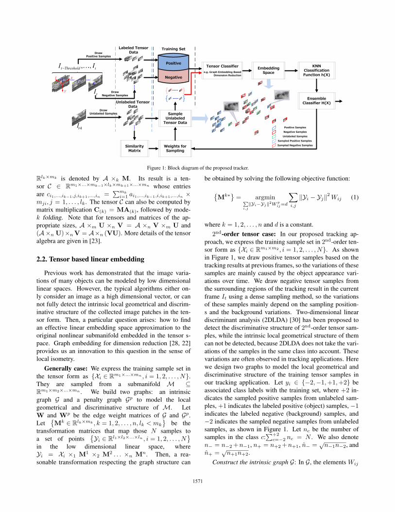
2. The Proposed Discriminant TrackingFigure 1 is an overview of the proposed approach. We

elaborate the important components of the proposed ap-

proach in this section, in particular the tensor based linear

embedding and derivation of the proposed semi-supervised

improvement technique. Before all of these, we first review

some terminology for tensor operations.

2.1. Terminology for tensor operations

A tensor is a higher order generalization of a vector (1st-order tensor) and a matrix (2nd-order tensor). A tensor is

a multilinear mapping over a set of vector spaces. An nth-

order tensor is denoted as A ∈ Rm1×m2×...×mn , and its

elements are represented by ai1,...,in . The inner product of

two nth-order tensors is defined as

〈A,B〉 =i1=m1,...,in=mn∑

i1=1,...,in=1

ai1,...,inbi1,...,in ,

the norm of A is ‖A‖ =√〈A,A〉, and the distance be-

tween A and B is ‖A − B‖. In the 2nd-order tensor case,

the norm is called the Frobenius norm and written as ‖A‖F .

The mode-k vectors are the column vectors of ma-

trix A(k) ∈ Rmk×(m1m2...mk−1mk+1...mn) that result-

s from flattening the tensor A. The inverse operation

of mode-k flattening is mode-k folding, which restores

the original tensor A from A(k). The mode-k produc-

t of a tensor A ∈ Rm1×m2×...×mn and a matrix M ∈

15701570

����

� �� ������� �� �� �� ���

��

Figure 1: Block diagram of the proposed tracker.

Rlk×mk is denoted by A ×k M. Its result is a ten-

sor C ∈ Rm1×...×mk−1×lk×mk+1×...×mn whose entries

are ci1,...,ik−1,j,ik+1,...,in =∑mk

i=1 ai1,...,ik−1,i,ik+1,...,in ×mji, j = 1, . . . , lk. The tensor C can also be computed by

matrix multiplication C(k) = MA(k), followed by mode-

k folding. Note that for tensors and matrices of the ap-

propriate sizes, A ×m U ×n V = A ×n V ×m U and

(A×n U)×nV = A×n (VU). More details of the tensor

algebra are given in [23].

2.2. Tensor based linear embedding

Previous work has demonstrated that the image varia-

tions of many objects can be modeled by low dimensional

linear spaces. However, the typical algorithms either on-

ly consider an image as a high dimensional vector, or can

not fully detect the intrinsic local geometrical and discrim-

inative structure of the collected image patches in the ten-

sor form. Then, a particular question arises: how to find

an effective linear embedding space approximation to the

original nonlinear submanifold embedded in the tensor s-

pace. Graph embedding for dimension reduction [28, 22]

provides us an innovation to this question in the sense of

local isometry.

Generally case: We express the training sample set in

the tensor form as {Xi ∈ Rm1×...×mn , i = 1, 2, . . . , N}.

They are sampled from a submanifold M ⊆R

m1×m2×...×mn . We build two graphs: an intrinsic

graph G and a penalty graph Gp to model the local

geometrical and discriminative structure of M. Let

W and Wp be the edge weight matrices of G and Gp.

Let{Mk ∈ R

lk×mk , k = 1, 2, . . . , n, lk < mk

}be the

transformation matrices that map those N samples to

a set of points{Yi ∈ R

l1×l2×...×ln , i = 1, 2, . . . , N}

in the low dimensional linear space, where

Yi = Xi ×1 M1 ×2 M2 . . . ×n Mn. Then, a rea-

sonable transformation respecting the graph structure can

be obtained by solving the following objective function:

{Mk∗} = argmin

∑

i,j‖Yi−Yj‖2Wp

ij=d

∑i,j

‖Yi − Yj‖2 Wij (1)

where k = 1, 2, . . . , n and d is a constant.

2nd-order tensor case: In our proposed tracking ap-

proach, we express the training sample set in 2nd-order ten-

sor form as {Xi ∈ Rm1×m2 , i = 1, 2, . . . , N}. As shown

in Figure 1, we draw positive tensor samples based on the

tracking results at previous frames, so the variations of these

samples are mainly caused by the object appearance vari-

ations over time. We draw negative tensor samples from

the surrounding regions of the tracking result in the current

frame It using a dense sampling method, so the variations

of these samples mainly depend on the sampling position-

s and the background variations. Two-dimensional linear

discriminant analysis (2DLDA) [30] has been proposed to

detect the discriminative structure of 2nd-order tensor sam-

ples, while the intrinsic local geometrical structure of them

can not be detected, because 2DLDA does not take the vari-

ations of the samples in the same class into account. These

variations are often observed in tracking applications. Here

we design two graphs to model the local geometrical and

discriminative structure of the training tensor samples in

our tracking application. Let yi ∈ {−2,−1,+1,+2} be

associated class labels with the training set, where +2 in-

dicates the sampled positive samples from unlabeled sam-

ples, +1 indicates the labeled positive (object) samples, −1indicates the labeled negative (background) samples, and

−2 indicates the sampled negative samples from unlabeled

samples, as shown in Figure 1. Let nc be the number of

samples in the class c:∑+2

c=−2 nc = N . We also denote

n− = n−2+n−1, n+ = n+2+n+1, n̂− =√n−1n−2, and

n̂+ =√n+1n+2.

Construct the intrinsic graph G: In G, the elements Wij

15711571

of W are defined as follows:

Wij =

⎧⎪⎪⎨⎪⎪⎩Aij/nc, if yi = yj = c,Aij/n̂+, elseif yi > 0 and yj > 0,Aij/n̂−, elseif yi < 0 and yj < 0,0, otherwise.

(2)

The affinity Aij is defined by the local scaling method

in [32]. Without loss of generality, we assume that the da-

ta points in {Xi}Ni=1 are ordered according to their labels

yi ∈ {−2,−1,+1,+2}. When yi > 0 and yj > 0,

Aij = exp(−‖Xi −Xj‖2/(σiσj)

), (3)

where σi =∥∥∥Xi −X (k)

i

∥∥∥, and X (k)i is the kth nearest

neighbor of Xi in {Xj}Nj=n−+1. When yi < 0 and yj < 0,

Aij =

{exp

(−‖Xi−Xj‖2

σiσj

), if i ∈ N+

k (j) or j ∈ N+k (i),

0, otherwise,

(4)

where N+k (i) indicates the index set of the k nearest neigh-

bors of Xi in {Xj}n−j=1, σi =∥∥∥Xi −X (k)

i

∥∥∥, and X (k)i is the

kth nearest neighbor of Xi in {Xj}n−j=1. The parameter kabove is empirically chosen as 7 based on [32].

Construct the penalty graph Gp: In Gp, the elements W pij

of Wp are defined as follows:

W pij =

⎧⎪⎪⎨⎪⎪⎩Aij (1/N − 1/nc) , if yi = yj = c,Aij (1/N − 1/n̂+) , elseif yi > 0 and yj > 0,Aij (1/N − 1/n̂−) , elseif yi < 0 and yj < 0,1/N, otherwise,

(5)

Note that we add the local isometry into the graph struc-

ture. Specifically, we determine the embedding space so

that, i) when yi · yj > 0, the nearby data pairs (large values

of Aij) are close and the data pairs far apart (small values

of Aij) are not required to be close; ii) when yi · yj < 0, the

data pairs are apart by imposing 1/N . In addition, when we

combine the sampled unlabeled samples with the labeled

samples to train a new classification model (see Algorith-

m 2) for improvement of original classifier, we increase

the contribution of the sampled unlabeled samples by two

means: i) imposing 1/nc, 1/n̂+ and 1/n̂− in Eq. (2) and

Eq. (5) (n−2 < n−1, n+2 < n+1 in general); ii) assigning

the labels +2 or −2 to the sampled unlabeled samples.

By some tensor operations, solving the objective func-

tion Eq. (1) in the 2nd-order tensor case is equivalent to

solving the following constrained optimization problem:

minimizeU,V

∑i,j

∥∥UTXiV −UTXjV∥∥2

FWij ,

subject to∑i,j

∥∥UTXiV −UTXjV∥∥2

FW p

ij = d(6)

where UT = M1, VT = M2, and d is a constant. Let

D and Dp be diagonal matrices, where Dii =∑

j Wij and

Dpii =

∑j W

pij . According to [7], the optimization problem

Eq. (6) can be further reformulated as either of the following

two optimization problems: minU,V

tr

(UT (DV −WV )U

UT (DpV −Wp

V )U

)or

minU,V

tr

(VT (DU−WU )V

VT (DpU−Wp

U)V

), where

DV =∑

i DiiXiVVTX Ti , WV =

∑i,j WijXiVVTX T

j ,

DpV =

∑i D

piiXiVVTX T

i , WpV =

∑i,j W

pijXiVVTX T

j ,

DU =∑

i DiiX Ti UUTXi, WU =

∑i,j WijX T

i UUTXj ,

DpU =

∑i D

piiX T

i UUTXi, WpU =

∑i,j W

pijX T

i UUTXj .

Algorithm 1 Online Tensor Classifier

Input: Training dataset {Xi, i = 1, 2, . . . , N}, and associated

class labels yi ∈ {−2,−1,+1,+2}.

Output: The linear embedding space projected from original

nonlinear submanifold with transformation matrices U, V.

1: Initially set U to the first l1 columns of I and set iteration ←1;

2: Calculate W and Wp from Eq. (2) and Eq. (5);

3: for iteration = 1→ T do4: Calculate DU , WU , Dp

U , WpU ;

5: Compute V by solving the generalized eigenvector prob-

lem: (DpU −Wp

U )v = λ (DU −WU )v;

6: Calculate DV , WV , DpV , Wp

V ;

7: Update U by solving the generalized eigenvector problem:

(DpV −Wp

V )u = λ (DV −WV )u;

8: end for9: KNN classifier h(X ) is used for classification in the linear

embedding space for its simplicity.

In Algorithm 1, we describe a commonly used compu-

tational method to solve the two minimization problems. It

has been empirically shown in [29, 7] that the iterative al-

gorithm converges to a satisfactory result within three itera-

tions. To simplify the efficiency analysis of Step 4 and 6 in

Algorithm 1, we assume l1 = l2 = l, and m1 = m2 = m.

The main cost is the calculations of WU , WV , WpU , Wp

V ,

each of which has O(N2(m2 + 2m2l)) floating-point mul-

tiplications. However, the sparsity of W and Wp make the

cost much lower.

2.3. Semi-supervised improvement

Recall that we model the local geometrical and discrim-

inative structure of the nonlinear submanifold M by build-

ing two graphs based on the manifold assumption. But the

correlations within matrix (in the 2nd-order tensor case) are

not limited to the elements along particular columns and

rows. The learned discriminative embedding space using

only the labeled samples may not encode enough of the dis-

criminant information. So we need to adjust the discrimi-

native embedding space to encode most of the discriminant

information. The cluster assumption allows us to use the

15721572

unlabeled data to do this. It states that the data samples

with high similarity between them, must share the same la-

bel. We define the objective function of the semi-supervised

improvement using the cluster assumption.

Let {Xi}Nl

i=1 denote the labeled tensor samples, and

{Xi}Nl+Nu

i=Nl+1 denote the unlabeled ones. Suppose that the

labeled ones are labeled by yl =(yl1, y

l2, . . . , y

lNl

), where

each class label yli is either +1 or −1. Let S = [Sij ]Ne×Ne

denote the symmetric similarity matrix, where Sij (Sij ≥0) represents the similarity between Xi and Xj , and Ne =Nl + Nu. In this paper, we use the block-division based

covariance matrix descriptor to measure the similarity un-

der log-Euclidean Riemannian metric (see [14]). We define

the distance between any two samples Xi and Xj under this

metric M as DM (Xi,Xj). Then the similarity Sij is de-

fined by Sij = exp(−D2

M (Xi,Xj) /(σiσj)), where σi has

the similar definition to that in Eq. (3).

We derive the semi-supervised improvement algorithm

using an iterative approach. Let h(0)(X ) : Rm1×m2 →

{−1,+1} denote the tensor classification model that is

learned by Algorithm 1 based on only the labeled sam-

ples. Let h(t)(X ) : Rm1×m2 → {−1,+1}, which is

used to improve the performance of h(0)(X ), denote the

one that is learned at the t-th iteration by Algorithm 1. Let

H(X ) : Rm1×m2 → R denote the linearly combined ten-

sor classification model learned after the first T̂ iterations:

H(X ) = α0h(0)(X ) +

∑T̂t=1 αth

(t)(X ), where α0 and αt

are the combination weights. At the (T̂+1)-st iteration, our

goal is to find a new tensor classifier h(X ) with the com-

bination weight α that can efficiently satisfy the following

optimization problem:

minimizeh(X ),α

Nl∑i=1

Ne∑j=Nl+1

Sijexp(−2yli(Hj + αhj)

)

+ C

Ne∑i,j=Nl+1

Sijexp (Hi −Hj) exp (α(hi − hj)) ,

subject to h (Xi) = yli, i = 1, . . . , Nl

(7)

where Hi ≡ H (Xi), hi ≡ h (Xi) and C weights the con-

tribution of the inconsistency among the unlabeled data. In

fact C is chosen to be C = Nl/Nu.

Note that the first term in Eq. (7) measures the inconsis-

tency between labeled and unlabeled samples, and the sec-

ond one measures the inconsistency among the unlabeled

samples. Unlabeled samples which are similar to a labeled

sample must share its label, and a set of similar unlabeled

samples must share the same label.

By regrouping the terms, we rewrite the optimization

problem Eq. (7) as the task of minimizing the function

F =∑Ne

i=Nl+1

(e−2αhipi + e2αhiqi

), where

Algorithm 2 Semi-supervised Improvement

Input: Labeled samples {Xi}Nli=1 and associated class labels yl,

unlabeled samples {Xi}Nei=Nl+1.

Output: The improved tensor classifier H(·).1: Compute the pairwise similarity Sij ;

2: Train h(0)(X ) by Algorithm 1 based on only {Xi}Nli=1;

3: Let H(·) = 0, and compute α0 using Eqs. (8) (9) (10);

4: Initialize H(X ) = α0h(0)(X );

5: for t = 1→ T̂ do6: Compute pi and qi for every unlabeled sample by E-

qs. (8) (9);

7: Sample the unlabeled samples by the weights |pi− qi|, and

label them with zi = 2 · sign(pi − qi);8: Combine the sampled samples with {Xi}Nl

i=1 to train a new

tensor classifier h(t)(X ) by Algorithm 1;

9: Compute αt using Eq. (10);

10: Improve the classification function as H(X ) ← H(X ) +αth

(t)(X );11: end for12: return H(X ) = α0h

(0)(X ) +∑T̂

t=1 αth(t)(X ).

pi =

Nl∑j=1

Sije−2Hiδ(ylj , 1) +

C

2

Ne∑j=Nl+1

SijeHj−Hi (8)

qi =

Nl∑j=1

Sije2Hiδ(ylj ,−1) +

C

2

Ne∑j=Nl+1

SijeHi−Hj (9)

and δ(x, y) = 1 when x = y and 0 otherwise. According

to [16], F is minimized when we choose h (X ) such that

the unlabeled samples with maximum values of |pi − qi|are classified by hi = sign(pi − qi). The optimal α that

minimizes F is

α =1

4ln

∑Nei=Nl+1 piδ(hi, 1) +

∑Nei=Nl+1 qiδ(hi,−1)∑Ne

i=Nl+1 piδ(hi,−1) +∑Ne

i=Nl+1 qiδ(hi, 1).

(10)

That is to say, at each iteration, we can sample these unla-

beled samples according to the weights |pi− qi|, label them

with zi = 2 · sign(pi − qi), and combine them with the

labeled samples (labeled with yl) to learn a new discrimi-

native embedding space and a new tensor classifier model

h (X ), obtained as shown in Figure 1. We detail the proce-

dure of the semi-supervised improvement in Algorithm 2.

Discussion From Eq. (8) and Eq. (9), we can see that,

if an unlabeled sample Xi is highly similar to the positive

samples, but wrongly predicted to have the negative label

by the un-improved tensor classifier, then this unlabeled

sample has a large pi and a small qi. We sample this un-

labeled sample and label it with zi = 2 · sign(pi−qi). Like-

wise, we sample the top few most “mispredicted” samples

for improving the original tensor classifier. All these sam-

pled unlabeled samples help to compensate for the loss of

discriminant information encoded in the embedding space

15731573

of the un-improved tensor classifier and to encode most of

the discriminant information. Grabner et al. [6] use similar

mechanism to weight the unlabeled samples and hence use

them to train their feature selection based boosting classifi-

er. Their method uses all the unlabeled samples for training

without selection. A direct comparison of results obtained

from their method and ours is given in Section 3.2.

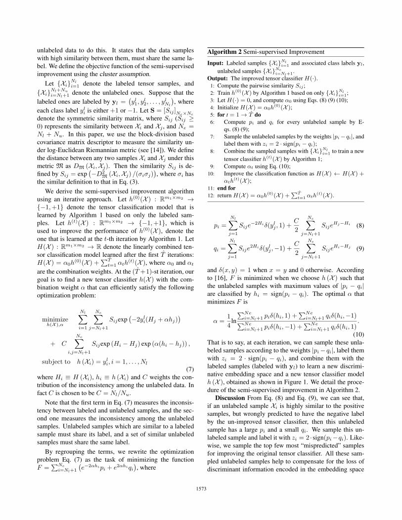
3. Experimental Results and AnalysisIn this section, we present experimental results that vali-

date the superior properties of our proposed tensor represen-

tation based discriminant tracker with semi-supervised im-

provement (SSI-TDT). As described in Section 1, we make

two novel assumptions for our tracking approach, which are

image-as-matrix assumption and semi-supervised improv-

ing assumption. With different assumptions, different ob-

ject trackers are obtained. When we adopt the image-as-

vector assumption, it is a vector representation based dis-

criminant tracker with semi-supervised improvement (SSI-

VDT). Our tracking approach without semi-supervised im-

proving assumption results in TDT. TDT with margin im-

proving assumption (e.g. ASSEMBLE) results in MI-TDT.

We compare SSI-TDT with SSI-VDT, TDT, and MI-TDT

to demonstrate the effectiveness of our assumptions. Addi-

tionally, we conduct a thorough comparison between SSI-

TDT and eight recent and state-of-the-art visual trackers de-

noted as: IRTSA [13], Frag [1], VTD [8], VTS [9], MIL [2],

IVT [21], and APG-�1 [3], SSOBT [6]. We implement these

trackers using publicly available source codes or binaries

provided by the authors. For fair evaluation, each tracker is

run with appropriately adjusted parameters.

Implementation details All our experiments are done

using MATLAB R2008b on a 2.83GHz Intel Core2 Quad

PC with 4GB RAM. As shown in Figure 1, we use the parti-

cle filter in [21] to draw unlabeled samples from frame It+1,

where we simply consider the object state information in 2D

translation and scaling, and set the number Nu of particles

to 600. We draw positive samples based on the tracking re-

sults at previous frames, and draw negative samples from

the current frame It using the dense sampling method. In

practice, we set the number of positive samples n+1 = 50,

the number of negative samples n−1 = 100. We sample top

10% of the unlabeled samples for improvement of original

classifier. This indicates that Nl = 150, and N = 210. All

the image regions corresponding to these samples are nor-

malized to templates of size 32 × 32, which indicates that

m1 = m2 = 32. The column number of U and V in Al-

gorithm 1 are both set to l1 = l2 = 2. The parameter T̂ in

Algorithm 2 is set to 2 for the sake of compromise between

tracking speed and accuracy. The above parameter settings

remain the same in all the experiments.

To evaluate SSI-TDT, we compile a set of 12 challeng-

ing video sequences consisting of 8-bit grayscale images.

�� �� �� �� �� � �

��

���

���

���

�

�

��� ��� �� ��� ���� ����

��

��

��

��

��

�

�

�

�� �� �� �� �� � ��

���

���

��

���

�

�

��� ��� �� ��� ���� �����

���

���

��

���

�

�

Figure 2: Quantitative comparison of the proposed tracker with different

assumptions on two videos. The left two subfigures are associated with the

tracking performance in CLE and VOR on the animal video, respectively;

the right two subfigures correspond to the tracking performance in CLE

and VOR on the sylv video, respectively.

animal boat coke11 david dudek football sylv womanSSI-TDT 0.94 0.81 0.80 0.99 1.00 0.73 0.88 0.87

TDT 0.44 0.27 0.83 0.29 0.58 0.60 0.79 0.59

MI-TDT 0.59 0.59 0.78 0.34 0.93 0.62 0.73 0.77

SSI-VDT 0.27 0.62 0.10 0.48 0.78 0.29 0.72 0.09

Table 1: Quantitative comparison of the proposed tracker with different

assumptions on eight videos. The table reports their tracking success rates.

These videos include challenging appearance variations due

to the changes in pose, illumination, scale, and the presence

of occlusion and cluttered background. For quantitative

comparison, two evaluation criteria are introduced, namely,

center location error (CLE) and VOC overlap ratio (VOR)

between the predicted bounding box Bp and ground truth

Bgt (manually labeled) such that VOR =area(Bp

⋂Bgt)

area(Bp

⋃Bgt)

. If

VOR is larger than 0.5, then the target is considered to be

successfully tracked. This can be used to evaluate the suc-

cess rate (i.e., #successframes#totalframes ) of any tracking approach.

3.1. The effectiveness of our approach

As previously claimed, 2nd-order tensor (image-as-

matrix) representation methods can retain more useful in-

formation than image-as-vector representation methods,

and the semi-supervised improvement technique can en-

hance the tensor based discriminant tracker much more than

margin improving techniques. To demonstrate the effective-

ness of our two assumptions, we design several experiments

on eight videos. Figure 2 quantitatively shows some ex-

perimental results of the proposed tracker with different as-

sumptions on two of the eight videos. Table 1 reports their

tracking success rates on the eight videos. From Figure 2

and Table 1, we can see that semi-supervised improvemen-

t (SSI) technique always enhances TDT, and the enhance-

ment is always much more notable than margin improving

15741574

�� �� �� �� �� � �

��

��

�

��

���

���

���

��

���

�

�

��� ��� ��� ��� ��� �� �� ����

��

���

���

���

�

�

��� ��� ��� ��� ��� ��

���

���

���

���

���

��

�

�

�� ��� ��� ��� ��� ��� ����

��

��

�

��

���

���

���

��

�

�

�� ��� ��� ��� ����

��

��

�

��

���

�

�

��� ��� ��� ����

��

���

���

�

�

�� ��� ��� ��� ��� ��� ����

��

���

���

���

�

�

�� ��� ��� ��� ��� ����

��

���

���

���

���

���

�

�

��� ��� �� ��� ���� �����

��

���

���

�

�

��� ��� ��� ��� ���

��

���

���

���

���

�

�

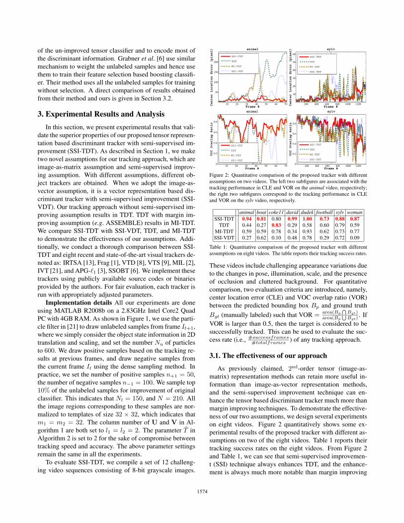
Figure 3: Quantitative comparison of different trackers in terms of CLE on ten videos.

(MI) technique’s, except for the coke11 video. The reason

is the coke11 video has few challenges in illumination, s-

cale changes and background clutter, while the challenges

caused by the presence of occlusion and varying viewpoints

are obviously noted. TDT can handle the later challenges

well, so SSI technique and MI technique are not required

in the coke11 video. TDT can’t handle the challenges in

large scale variation (e.g. david, dudek), background clut-

ter (e.g. boat, football), fast motion and blur (e.g. animal)well. In addition, although the SSI technique and discrim-

inant information are used, the image-as-vector representa-

tion based tracker (SSI-VDT) still can’t meet the challenges

caused by the presence of occlusion (e.g. coke11, football,woman), fast motion and blur (e.g. animal) well because of

the limitations of image-as-vector representation.

3.2. Comparison with competing trackers

To show the superiority of SSI-TDT over other compet-

ing trackers, we perform experiments using IRTSA [13],

Frag [1], VTD [8], VTS [9], MIL [2], IVT [21], APG-�1 [3]

and SSOBT [6] on twelve videos. Figure 3 shows the center

location errors of the nine evaluated trackers on ten videos.

Table 2 and Table 3 summarize the average center location

errors in pixels and the success rates over all the twelve

videos, respectively. Over all, the proposed tracking ap-

proach performs favorably against state-of-the-art trackers.

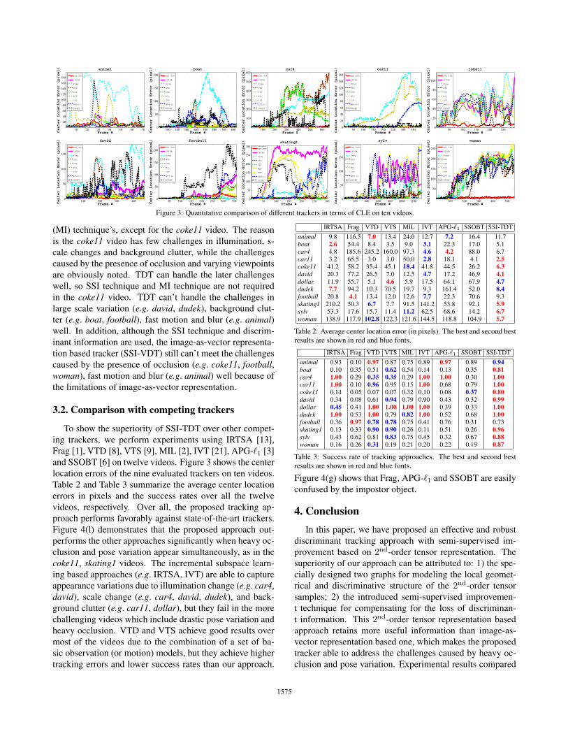
Figure 4(l) demonstrates that the proposed approach out-

performs the other approaches significantly when heavy oc-

clusion and pose variation appear simultaneously, as in the

coke11, skating1 videos. The incremental subspace learn-

ing based approaches (e.g. IRTSA, IVT) are able to capture

appearance variations due to illumination change (e.g. car4,

david), scale change (e.g. car4, david, dudek), and back-

ground clutter (e.g. car11, dollar), but they fail in the more

challenging videos which include drastic pose variation and

heavy occlusion. VTD and VTS achieve good results over

most of the videos due to the combination of a set of ba-

sic observation (or motion) models, but they achieve higher

tracking errors and lower success rates than our approach.

IRTSA Frag VTD VTS MIL IVT APG-�1 SSOBT SSI-TDT

animal 9.8 116.5 7.0 13.4 24.0 12.7 7.2 16.4 11.7boat 2.6 54.4 8.4 3.5 9.0 3.1 22.3 17.0 5.1car4 4.8 185.6 245.2 160.0 97.3 4.6 4.2 88.0 6.7car11 3.2 65.5 3.0 3.0 50.0 2.8 18.1 4.1 2.5coke11 41.2 58.2 35.4 45.1 18.4 41.8 44.5 26.2 6.3david 20.3 77.2 26.5 7.0 12.5 4.7 17.2 46.9 4.1dollar 11.9 55.7 5.1 4.6 5.9 17.5 64.1 67.9 4.7dudek 7.7 94.2 10.3 70.5 19.7 9.3 161.4 52.0 8.4football 20.8 4.1 13.4 12.0 12.6 7.7 22.3 70.6 9.3skating1 210.2 50.3 6.7 7.7 91.5 141.2 53.8 92.1 5.9sylv 53.3 17.6 15.7 11.4 11.2 62.5 68.6 14.2 6.7woman 138.9 117.9 102.8 122.3 121.6 144.5 118.8 104.9 5.7

Table 2: Average center location error (in pixels). The best and second best

results are shown in red and blue fonts.

IRTSA Frag VTD VTS MIL IVT APG-�1 SSOBT SSI-TDT

animal 0.93 0.10 0.97 0.87 0.75 0.89 0.97 0.89 0.94boat 0.10 0.35 0.51 0.62 0.54 0.14 0.13 0.35 0.81car4 1.00 0.29 0.35 0.35 0.29 1.00 1.00 0.30 1.00car11 1.00 0.10 0.96 0.95 0.15 1.00 0.68 0.79 1.00coke11 0.14 0.05 0.07 0.07 0.32 0.10 0.08 0.37 0.80david 0.34 0.08 0.61 0.94 0.79 0.90 0.43 0.32 0.99dollar 0.45 0.41 1.00 1.00 1.00 1.00 0.39 0.33 1.00dudek 1.00 0.53 1.00 0.79 0.82 1.00 0.52 0.68 1.00football 0.36 0.97 0.78 0.78 0.75 0.41 0.76 0.31 0.73skating1 0.13 0.33 0.90 0.90 0.26 0.11 0.51 0.26 0.96sylv 0.43 0.62 0.81 0.83 0.75 0.45 0.32 0.67 0.88woman 0.16 0.26 0.31 0.19 0.21 0.20 0.22 0.19 0.87

Table 3: Success rate of tracking approaches. The best and second best

results are shown in red and blue fonts.

Figure 4(g) shows that Frag, APG-�1 and SSOBT are easily

confused by the impostor object.

4. ConclusionIn this paper, we have proposed an effective and robust

discriminant tracking approach with semi-supervised im-

provement based on 2nd-order tensor representation. The

superiority of our approach can be attributed to: 1) the spe-

cially designed two graphs for modeling the local geomet-

rical and discriminative structure of the 2nd-order tensor

samples; 2) the introduced semi-supervised improvemen-

t technique for compensating for the loss of discriminan-

t information. This 2nd-order tensor representation based

approach retains more useful information than image-as-

vector representation based one, which makes the proposed

tracker able to address the challenges caused by heavy oc-

clusion and pose variation. Experimental results compared

15751575

(a) animal (b)boat (c)car4

(d)car11 (e)coke11 (f)david

(g)dollar (h)dudek (i) football

(j) skating1 (k) sylv (l)womanIRTSA Frag VTD VTS MIL IVT SSI-TDTAPG-L1 SSOBT

Figure 4: Screenshots of some sampled tracking results of evaluated approaches on twelve challenging videos.

with several state-of-the-art trackers on challenging videos

demonstrate the effectiveness and robustness of the pro-

posed approach.

Acknowledgment This work is partly supported by NS-

FC (Grant No. 60935002), the National 863 High-Tech

R&D Program of China (Grant No. 2012AA012504),

the Natural Science Foundation of Beijing (Grant No.

4121003), and The Project Supported by Guangdong Natu-

ral Science Foundation (Grant No. S2012020011081).

References[1] A. Adam, E. Rivlin, and I. Shimshoni. Robust fragments-based tracking using

the integral histogram. In CVPR, 2006.

[2] B. Babenko, M. Yang, and S. Belongie. Visual tracking with online multipleinstance learning. In CVPR, 2009.

[3] C. Bao, Y. Wu, H. Ling, and H. Ji. Real time robust �1 tracker using acceleratedproximal gradient approach. In CVPR, 2012.

[4] K. P. Bennett, A. Demiriz, and R. Maclin. Exploiting unlabeled data in ensem-ble methods. In ACM SIGKDD, 2002.

[5] H. Grabner, M. Grabner, and H. Bischof. Real-time tracking via on-line boost-ing. In BMVC, 2006.

[6] H. Grabner, C. Leistner, and H. Bischof. Semi-supervised on-line boosting forrobust tracking. In ECCV, 2008.

[7] X. He, D. Cai, and P. Niyogi. Tensor subspace analysis. In NIPS, 2005.

[8] J. Kwon and K. Lee. Visual tracking decomposition. In CVPR, 2010.

[9] J. Kwon and K. Lee. Tracking by sampling trackers. In ICCV, 2011.

[10] G. Li, L. Qin, Q. Huang, J. Pang, and S. Jiang. Treat samples differently: objecttracking with semi-supervised online covboost. In ICCV, 2011.

[11] P. Li and Q. Sun. Tensor-based covariance matrices for object tracking. InICCV Workshops, 2011.

[12] X. Li, A. Dick, H. Wang, C. Shen, and A. van den Hengel. Graph mode-basedcontextual kernels for robust svm tracking. In ICCV, 2011.

[13] X. Li, W. Hu, Z. Zhang, X. Zhang, and G. Luo. Robust visual tracking basedon incremental tensor subspace learning. In ICCV, 2007.

[14] X. Li, W. Hu, Z. Zhang, M. Zhu, and J. Cheng. Visual tracking via incrementallog-euclidean riemannian subspace learning. In CVPR, 2008.

[15] X. Li, C. Shen, Q. Shi, A. Dick, and A. van den Hengel. Non-sparse linearrepresentations for visual tracking with online reservoir metric learning. InCVPR, 2012.

[16] P. K. Mallapragada, R. Jin, A. K. Jain, and Y. Liu. Semiboost: Boosting forsemi-supervised learning. Trans. on PAMI, 31:2000–2014, 2009.

[17] X. Mei and H. Ling. Robust visual tracking using �1 minimization. In ICCV,2009.

[18] X. Mei, H. Ling, Y. Wu, E. Blasch, and L. Bai. Minimum error bounded effi-cient �1 tracker with occlusion detection. In CVPR, 2011.

[19] F. Porikli, O. Tuzel, and P. Meer. Covariance tracking using model update basedon lie algebra. In CVPR, 2006.

[20] C. Rosenberg, M. Hebert, and H. Schneiderman. Semi-supervised self-trainingof object detection models. In Workshop on Applications of Computer Vision,2005.

[21] D. A. Ross, J. Lim, R. Lin, and M. Yang. Incremental learning for robust visualtracking. Int. J. Comp. Vis., 77(1):125–141, 2008.

[22] M. Sugiyama. Dimensionality reduction of multimodal labeled data by localfisher discriminant analysis. Machine Learning Research, 8, 2007.

[23] M. A. O. Vasilescu and D. Terzopoulos. Tensor textures: multilinear image-based rendering. In ACM SIGGRAPH, 2004.

[24] Q. Wang, F. Chen, and W. Xu. Tracking by third-order tensor representation.Trans. on SMCB, 41(2):385–396, 2011.

[25] J. Wen, X. Gao, X. Li, and D. Tao. Incremental learning of weighted tensorsubspace for visual tracking. In Int. Conf. on Sys., Man, and Cyb., 2009.

[26] Y. Wu, J. Cheng, J. Wang, and H. Lu. Real-time visual tracking via incrementalcovariance tensor learning. In ICCV, 2009.

[27] S. Yan, D. Xu, S. Lin, T. S. Huang, and S. F. Chang. Element rearrangementfor tensor-based subspace learning. In CVPR, 2007.

[28] S. Yan, D. Xu, B. Zhang, H. Zhang, Q. Yang, and S. Lin. Graph embeddingand extensions: A general framework for dimensionality reduction. Trans. onPAMI, 29:40–51, 2007.

[29] J. Ye. Generalized low rank approximations of matrices. Machine Learning,61:167–191, 2005.

[30] J. Ye, R. Janardan, and Q. Li. Two-dimensional linear discriminant analysis. InNIPS, 2004.

[31] A. Yilmaz, O. Javed, and M. Shah. Object tracking: A survey. ACM ComputingSurveys, 38(4):13, 2006.

[32] L. Zelnik-Manor and P. Perona. Self-tuning spectral clustering. In NIPS, 2005.

[33] T. Zhang, B. Ghanem, S. Liu, and N. Ahuja. Low-rank sparse learning forrobust visual tracking. In ECCV, 2012.

[34] T. Zhang, B. Ghanem, S. Liu, and N. Ahuja. Robust visual tracking via multi-task sparse learning. In CVPR, 2012.

[35] X. Zhang, W. Hu, S. Maybank, and X. Li. Graph based discriminative learningfor robust and efficient object tracking. In ICCV, 2007.

15761576