Discrete Speed in Vertical Flight Planning

Zhi Yuan1, Liana Amaya Moreno1, Armin Fugenschuh1, Anton Kaier2, andSwen Schlobach2

1 Professorship of Applied Mathematics, Department of Mechanical Engineering,Helmut Schmidt University, Hamburg, Germany{yuanz,fuegenschuh,lamayamo}@hsu-hh.de

2 Lufthansa Systems AG, Kelsterbach, Germany{anton.kaier,swen.schlobach}@lhsystems.com

Abstract. Vertical flight planning concerns assigning optimal cruise al-titude and speed to each trajectory-composing segment, such that thefuel consumption is minimized, and the arrival time constraints are sat-isfied. The previous work that assigns continuous speed to each segmentleads to prohibitively long computation time. In this work, we propose amixed integer linear programming model that assigns discrete speed. Inparticular, an all-but-one speed discretization scheme is found to scalewell with problem size with only negligible objective deviation from usingcontinuous speed. Extensive experiments with real-world instances haveshown the practical effectiveness and feasibility of the proposed speeddiscretization approach.

Keywords: Flight planning; mixed integer programming; variable dis-cretization; piecewise linear interpolation

1 Introduction

Air transport is an important component of many international logistics net-works, including transportation of goods and people. Planning a fuel-efficienttrajectory for each flight is a practically important and computationally hardoptimization problem. Such a flight trajectory is in general four-dimensional(4D), which consists of horizontally a 2D route on the earth surface, vertically,a number of discrete admissible altitude levels, and a time dimension controlledby aircraft speed such that the flight can arrive within a certain strict time win-dow. Due to the computational difficulty of such a 4D optimization problem, inpractice, it is usually approached in two separate phases [2]: a horizontal opti-mization phase that searches for a trajectory on the earth surface consisting ofa set of segments, to which an optimal altitude and speed is assigned to in thesubsequent vertical optimization phase.

In this work, we focus on the vertical flight planning problem. The verticalprofile of a flight includes five stages: take-off, climb, cruise, descend, and land-ing. Here we focus on the cruise stage, since it consumes the most fuel and timeduring a flight, while the other stages are relatively short and usually have fixedprocedures due to safety considerations, which leaves little flexibility for fuel

2 Yuan, Fugenschuh, Amaya Moreno, Kaier, and Schlobach

optimization. Computing an optimal altitude profile in the absence of wind canalso provide estimated altitude for the 2D horizontal trajectory optimization [12].Such a steady-atmosphere optimal altitude profile increases approximately lin-early as fuel burns, however, it becomes irregular if altitude-dependent wind isconsidered [9]. A recent research by Lovegren and Hansman [10] confirmed a po-tential fuel saving of up to 3.5% by reassigning only altitude and speed to fixedflight trajectories, based on a study of 257 real flight operations in US. However,no time constraint is taken into account in their computation as in real-worldairline operations. In such case, there exists a backward dynamic programmingapproach to compute fuel-optimal vertical profile [17].

A practical challenge in airline operations is to handle time constraints, es-pecially delays, due to disruptions such as undesirable weather conditions, un-expected maintenance requirements, or waiting for passengers transferring fromother already delayed flights. Such delays are typically recovered by increasingcruise speed, such that the next connection for passengers as well as for the air-craft and the crew can be reached [1]. Varying cruise speed may also be useful,e.g., to enter a time-dependent restricted airspace before it is closed (or afterit is open), or when an aircraft is reassigned to a flight that used to be servedby a faster (or slower) aircraft. The industrial standard suggests using a costindex procedure to vary cruise speed. This requires inputing a value that reflectsthe importance between time-related cost and fuel-related cost. The use of costindex was criticized due to the difficulty to quantify the time-related cost in thepresence of delay, thus a dynamic cost index approach has been proposed to thisend [6]. However, such approach still cannot handle explicitly hard time con-straints, such as the about-to-close airspace. Akturk et al. [1] formulate the timeconstraint explicitly into their MIP model in the context of aircraft rescheduling.Their model uses only constant speed. Yuan et al. [18, 17] explicitly include thetime constraint and the use of variable speed in the vertical flight planning.

In [18, 17], the vertical flight planning problem with variable continuous speedis identified as a mixed-integer second-order cone programming (MISOCP) prob-lem. The second-order cone constraints consist in calculating the flight time, andthe integer variables consist in the 2D piecewise linear interpolation of the fuelconsumption function, as well as the selection of discrete admissible altitude lev-els. The MISOCP model is reformulated as a mixed-integer linear programmingmodel by applying linear approximation techniques [4, 8] and various piecewiselinear approximation techniques. Despite the performance boost by using thelinear approximation of the MISOCP model, the long computation time stillprevents it from being a practically feasible approach.

In this present work, we study an alternative model for the vertical flightplanning problem with discrete speed, i.e., only a set of speed levels can be se-lected for each segment. The use of speed discretization replaces the quadraticcone constraints by linear constraints, and it also reduces the 2D piecewise lin-ear fuel function to 1D, at the expense of introducing more binary variables.We experimentally investigate the computation scalability of the discrete speedmodel, and carefully analyze the discretization error that leads to differences in

Discrete Speed in Vertical Flight Planning 3

the objective value. In particular, to balance the computational scalability andthe discretization error, an all-but-one discretization, which discretizes speed onall but one segments, appears to be the most practically viable approach.

2 Vertical Flight Planning: The Problem Description

In the vertical flight planning problem (VFP), we are given a set of segmentsthat compose the flight trajectory. The wind information for each segment isgiven in both the track direction (flight direction) and cross-track direction. Thetask is to assign an altitude and a speed to each segment, such that the flightconsumes the least fuel while the arrival time constraints are satisfied. The alti-tude and the speed on each segment are invariant, and they can only be changedat the beginning of each segment, due to safety requirements. The cruise stageunder consideration in this work starts after the initial climb has brought theaircraft above the crossover altitude of around 29 000 feet. Depending on theflight direction (eastwards or westwards), a set of discrete admissible flight alti-tudes are allowed. We consider IFR RVSM flight levels [13], where two adjacentflight levels usually differ by 1 000 feet, and the eastwards and westwards flightsare allowed to fly in alternate flight levels.

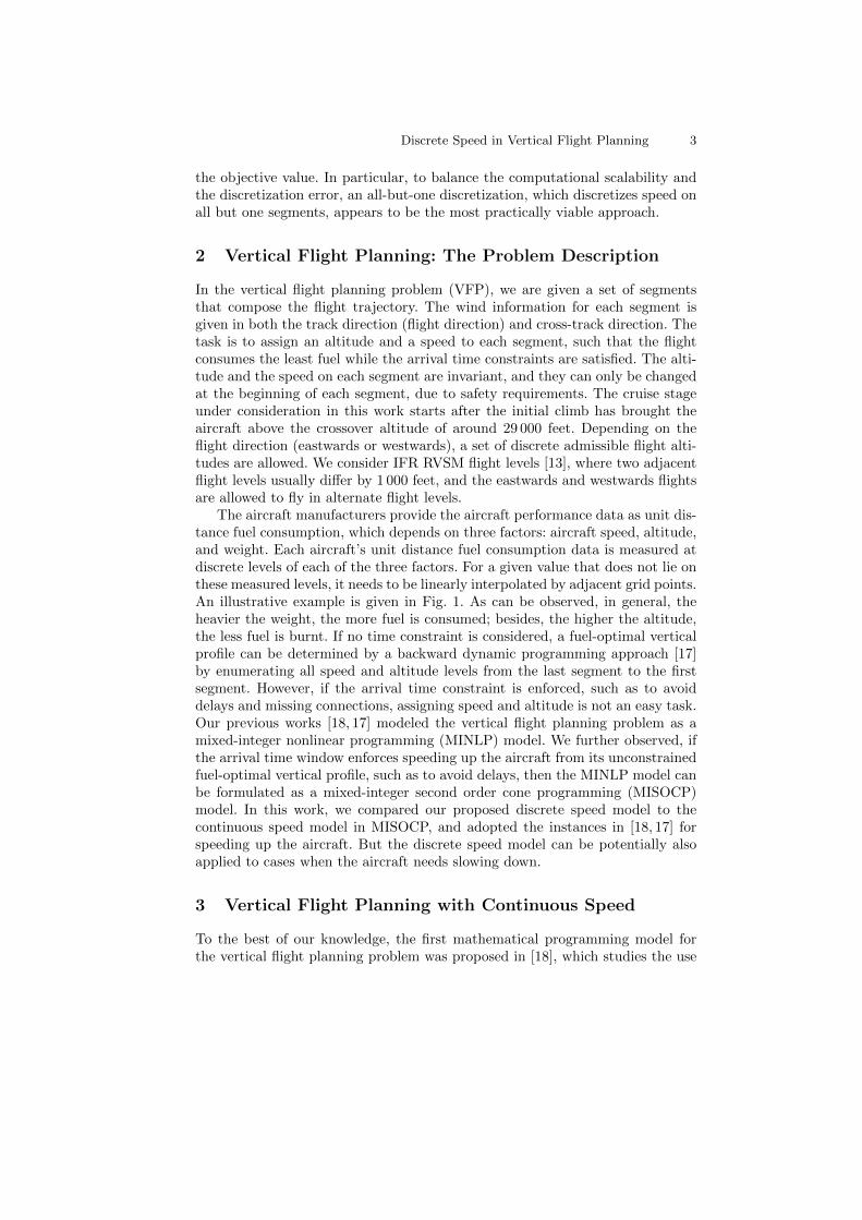
The aircraft manufacturers provide the aircraft performance data as unit dis-tance fuel consumption, which depends on three factors: aircraft speed, altitude,and weight. Each aircraft’s unit distance fuel consumption data is measured atdiscrete levels of each of the three factors. For a given value that does not lie onthese measured levels, it needs to be linearly interpolated by adjacent grid points.An illustrative example is given in Fig. 1. As can be observed, in general, theheavier the weight, the more fuel is consumed; besides, the higher the altitude,the less fuel is burnt. If no time constraint is considered, a fuel-optimal verticalprofile can be determined by a backward dynamic programming approach [17]by enumerating all speed and altitude levels from the last segment to the firstsegment. However, if the arrival time constraint is enforced, such as to avoiddelays and missing connections, assigning speed and altitude is not an easy task.Our previous works [18, 17] modeled the vertical flight planning problem as amixed-integer nonlinear programming (MINLP) model. We further observed, ifthe arrival time window enforces speeding up the aircraft from its unconstrainedfuel-optimal vertical profile, such as to avoid delays, then the MINLP model canbe formulated as a mixed-integer second order cone programming (MISOCP)model. In this work, we compared our proposed discrete speed model to thecontinuous speed model in MISOCP, and adopted the instances in [18, 17] forspeeding up the aircraft. But the discrete speed model can be potentially alsoapplied to cases when the aircraft needs slowing down.

3 Vertical Flight Planning with Continuous Speed

To the best of our knowledge, the first mathematical programming model forthe vertical flight planning problem was proposed in [18], which studies the use

4 Yuan, Fugenschuh, Amaya Moreno, Kaier, and Schlobach

Fig. 1. Unit distancefuel consumption withrespect to aircraftweight (in kg), altitude(in feet), and speed (inMach number).

of variable speed during a flight in the absence of wind. This model is furtherextended in [17] to include wind. Both models assign continuous speed to eachsegment, and can be identified as mixed integer second-order cone programming(MISCOP), if the aircraft needs to be speeded up. These two models are brieflypresented in this section.

3.1 Vertical Flight Planning without Wind (VFP-C)

In [18], a mathematical model for vertical flight planning without wind (VFP-C)is presented as follows. The unit distance fuel consumption F of an aircraft isgiven as measured data at discrete levels of the three dependent factors: speedV , altitude H, and weight W , as illustrated in Figure 1. If no wind is considered,given speed and weight, the optimal altitude can be precomputed by checkingall possible altitudes, thus it is not necessary to include its computation in theoptimization model. Other input parameters include a set of n segments S :={1, . . . , n} with length Li for all i ∈ S; the minimum and maximum trip durationT and T ; and the dry aircraft weight W dry, i.e. the weight of a loaded aircraftwithout trip fuel (reserve fuel for safety is included in the dry weight). Thevariables include the time vector ti for i ∈ S ∪ {0}, where ti−1 and ti denotethe start and end time of segment i; the travel time ∆ti spent on a segmenti ∈ S; the weight vector wi for i ∈ S∪{0} and wmid

i for i ∈ S where wi−1, wmidi ,

and wi denote the start, middle, and end weight at a segment i; the speed vion a segment i ∈ S; and the fuel fi consumed on a segment i ∈ S. A generalmathematical model for VFP-C can be stated as follows:

min w0 − wn (1)

s.t. t0 = 0, T ≤ tn ≤ T (2)

Discrete Speed in Vertical Flight Planning 5

∀i ∈ S : ∆ti = ti − ti−1 (3)

∀i ∈ S : Li = vi ·∆ti (4)

wn = W dry (5)

∀i ∈ S : wi−1 = wi + fi (6)

∀i ∈ S : wi−1 + wi = 2 · wmidi (7)

∀i ∈ S : fi = Li · F (vi, wmidi ). (8)

The objective function (1) minimizes the total fuel consumption measured bythe difference of aircraft weight before and after the flight; (2) ensures the flightduration within a given interval; time consistency is preserved by (3); the basicequation of motion (4) is enforced on each segment; (5) initializes the weightvector by assuming all trip fuel is burnt during the flight; weight consistency isensured in (6), and the middle weight of each segment calculated in (7) will be

used in the calculation of fuel consumption of each segment in (8), where F (v, w)is a piecewise linear function interpolating F for all the continuous values of vand w within the given grid of V ×W . F can be formulated as a MILP submodelusing Dantzig’s convex combination method [7, 16], a.k.a. lambda method. Ourprevious work [18] presents a variant of the 2D lambda method tailored for thisproblem. The quadratic constraint (4) can also be formulated as second-ordercone constraint, if the time constraint (2) requires the aircraft to speed up fromits unconstrained fuel-optimal travel time. A variable transformation techniqueto formulate it into a standard second-order cone constraint is presented in[18]. The resulting MISOCP can be solved by applying the linear approximationformulation for the second-order cone constraints that was proposed by Ben-Taland Nemirovski [4] and refined by Glineur [8] (see [18] for more details).

3.2 Vertical Flight Planning with Wind (VFPW-C)

In practice, wind plays an important roll in planning a fuel-optimal flight tra-jectory. In vertical flight planning, the wind also depends on the flight altitude.Since the segments S are given, the track wind component U t

i,h, i.e., the wind inthe flight direction, as well as the cross-track wind component U c

i,h, i.e., the windperpendicular to the flight direction, can be precomputed for each segment i ateach altitude h. The mathematical model without wind presented in Section 3.1is extended in [17] to include wind influence. Firstly, a further binary variableµi,h is introduced to indicate whether a segment i is flown on altitude h. Then

∀i ∈ S :∑h∈H

µi,h = 1 (9)

guarantees only one altitude is assigned to each segment. With the help of vari-able µ, the wind can be assigned to each segment by

∀i ∈ S : uti =∑h∈H

µi,h · U ti,h, (10)

6 Yuan, Fugenschuh, Amaya Moreno, Kaier, and Schlobach

∀i ∈ S : uci =∑h∈H

µi,h · U ci,h. (11)

The equation of motion (4) is reformulated based on the wind triangle (Figure 2):

Fig. 2. Wind triangle. vground

denotes the ground speed; vair

denotes the aircraft speed; vt

and ut denote the aircraft speedand wind speed in the track di-rection, respectively; uc denotesthe cross-track wind speed.

∀i ∈ S : Li = vgroundi ·∆ti (12)

∀i ∈ S : vgroundi = vti + uti (13)

∀i ∈ S : (vairi )2 = (vti)2 + (uci )

2. (14)

The two quadratic constraints (12) and (14) can be transformed into second-order cone if speeding up the aircraft is enforced, and thus can be reformulatedby linear approximation [17]. Furthermore, the fuel consumption per segment in(8) should be reformulated using the air speed and air distance as

∀i ∈ S : fi =∑h∈H

µi,h · FLi,h(vairi , wmid

i ), (15)

where FLi,h(v, w) denotes the fuel consumed by flying a segment i on an altitude

h, which can be computed in the preprocessing phase by

∀(v, w) ∈ V ×W : FLi,h(v, w) = F (v, w) · Li ·

v√v2 − (U c

i,h)2 + U ti,h

based on the wind triangle. FLi,h(v, w) is the 2D piecewise linear interpolation of

the data FLi,h(v, w) for all continuous values of (v, w) in the grid of V ×W , and

thus can be solved by the 2D piecewise linear function techniques. In particular,the lambda method is found to outperform the delta method for this model [17].

4 Speed Discretization in Vertical Flight Planning

The continuous speed models introduced in Section 3 can be classified as mixed-integer second-order cone programming models. The drawback of such modelsis their unpractically long computation time. In this section, another modelingalternative by discretizing the aircraft speed is presented.

Discrete Speed in Vertical Flight Planning 7

4.1 Discrete Speed in VFP without Wind (VFP-D)

We first focus on the vertical flight planning model without wind. Given a dis-crete set of aircraft speed V , we can further introduce binary variables µi,v,which indicates whether a discrete speed level v is used when flying on segmenti. Then only one speed level can be assigned to each segment by

∀i ∈ S :∑v∈V

µi,v = 1. (16)

With the discretized speed, the travel time ∆Ti,v for segment i with speed v canbe calculated in preprocessing,

∀i ∈ S, v ∈ V : ∆Ti,v =Li

v,

such that the quadratic constraint (4) can be linearized as:

∀i ∈ S : ∆t =∑v∈V

µi,v ·∆Ti,v. (17)

Besides, the 2D matrix F (v, w) can be reduced to Fv(w) of 1D by precomputing:

∀v ∈ V : Fv(w) = F (v, w),

such that the fuel consumption (8) can be reformulated as

∀i ∈ S : fi = Li ·∑v∈V

µi,v · Fv(wmidi ). (18)

Therefore, the speed discretization is the “stone that kills two birds”: it linearizesthe quadratic travel time constraint and reduces the 2D piecewise linear fuelfunction to 1D.

4.2 Discrete Speed in VFP with Wind (VFPW-D)

Similarly as in the VFP-D model in Section 4.1, speed discretization can help tosimplify the travel time equation as well as the fuel interpolation in the VFPW-C model. Firstly, the binary variables µi,h in the VFPW-C model are extendedto µi,h,v by one more dimension v ∈ V . Then (9) is replaced by

∀i ∈ S :∑

h∈H,v∈V

µi,h,v = 1 (19)

to ensure only one altitude and one speed level is assigned to each segment. Thenthe travel time ∆Ti,h,v for a segment i traveled on altitude h with speed v canbe precomputed based on the wind triangle:

∀i ∈ S, h ∈ H, v ∈ V : ∆Ti,h,v =Li√

v2 − (U ci,h)2 + U t

i,h

.

8 Yuan, Fugenschuh, Amaya Moreno, Kaier, and Schlobach

Then the travel time computation given by (12, 13, 14) can be simply replacedby linear constraint

∀i ∈ S : ∆t =∑

h∈H,v∈V

µi,h,v ·∆Ti,h,v. (20)

And replacing 2D matrix FLi,h(v, w) by 1D vector FL

i,h,v(w) as

∀v ∈ V : FLi,h,v(w) = FL

i,h(v, w),

reduces the 2D piecewise linear function (15) by one dimension:

∀i ∈ S : fi =∑

h∈H,v∈V

µi,h,v · FLi,h,v(wmid

i ), (21)

4.3 Univariate Piecewise Linear Interpolation

Here we review three different techniques to model the univariate piecewise linearfunction such as Fv and FL

i,h,v into mixed integer linear programming. Despitebeing mathematically equivalent (in the sense that they all describe the sameset of feasible solutions), their performances in terms of computation time areproblem dependent. Given an index set K0 := {0, 1, . . . ,m}, and the values forthe parameters W0 := {w0, w1, . . . , wm} are specified as F (wk) for k ∈ K0. Wefurther denote K := K0 \ {0} for the index set of intervals. A piecewise linear

function F : [w0, wm]→ R interpolating F can be modeled as follows.The Convex Combination (Lambda) Method. A variant of the convexcombination or lambda method [7] can be formulated as follows. To interpolate Fwe introduce binary decision variables τk ∈ {0, 1} for each k ∈ K, and continuousdecision variables λlk, λ

rk ∈ [0, 1] for each k ∈ K.∑

k∈K

τk = 1 (22a)

∀ k ∈ K : λlk + λrk = τk (22b)

w =∑k∈K

(wk−1 · λlk + wk · λrk) (22c)

F (w) =∑k∈K

(F (wk−1) · λlk + F (wk) · λrk) (22d)

Note that our variant uses twice as many lambda variables compared to theoriginal version of Dantzig [7], but in our numerical experiments it turned outthat problem instances can be solved significantly faster.The Special Ordered Set of Type 2 (SOS2) Method. Instead of intro-ducing decision variables for the selection of a particular interval (the τk above),we mark the lambda variables as belonging to a special ordered set of type 2(SOS2). That is, from an ordered set (or list) of variables (λ0, λ1, . . . , λm) it is

Discrete Speed in Vertical Flight Planning 9

required, that at most two of them are positive, and these two have to be adja-cent with respect to the ordering. This information is implicitly treated by thesolver in the solution process when branching on such special ordered set. SOS2branching was introduced by Beale and Tomlin [3]. We introduce continuousdecision variables 0 ≤ λk ≤ 1 for each k ∈ K0, and the following constraints:

SOS2(λ0, λ1, . . . , λm) (23a)

w =∑k∈K

(wk−1 · λk−1 + wk · λk) (23b)

F (w) =∑k∈K

(F (wk−1) · λk−1 + F (wk) · λk) (23c)

The Incremental (Delta) Method. The incremental (delta) method is theoldest of the three, introduced by Markowitz and Manne [11]. It uses binarydecision variable τk ∈ {0, 1} for k ∈ K and continuous decision variables δk ∈[0, 1] for k ∈ K, and the following constraints:

∀ k ∈ K : τk ≥ δk (24a)

∀ k ∈ K \ {n} : δk ≥ τk+1 (24b)

w = w0 +∑k∈K

(wk − wk−1) · δk (24c)

F (w) = F (w0) +∑k∈K

(F (wk)− F (wk−1)) · δk (24d)

4.4 All-but-one Speed Discretization

Variable discretization often leads to a discretization error and thus a loss ofoptimality in the objective value. In particular, when an aircraft needs speedingup, the shorter the flight time, the more fuel is consumed. Thus it is usuallyfuel-optimal to arrive at the exact arrival time upper bound. But this is usuallynot possible with discretized speed as it is with continuous speed. Therefore, itmay result in an unnecessary speedup on some segments, and the speed on somesegments may need to be adjusted from its optimal setting in order to arrive asclose to the prescribed time boundary as possible. This problem can be solvedby leaving one segment with continuous speed while discretizing the speed forall other segments. More specifically, we pick the last segment to use continuousspeed by the method described in Section 3, and the discrete speed is used onthe rest of the segments and solved as described in this section.

5 Experimental Results

5.1 Experimental Setup

Two of the most common aircraft types, Airbus 320 (A320) and Boeing 737(B737), are used for the empirical studies in this work. The aircraft performance

10 Yuan, Fugenschuh, Amaya Moreno, Kaier, and Schlobach

data and the upper air data are provided by Lufthansa Systems AG. Two ver-tical flight planning problems are considered, the one without wind (VFP), andthe other with wind (VFPW). For VFP, the instances considered in [18] forcontinuous speed are adopted here, including two speedup factors (flying 2.5%and 5% faster than unconstrained optimal). Five instances sizes are consideredfor A320, ranging from 15, 20, 25, 30, and 35 segments, each of which is 100nautical miles (NM) long,3 which results in flight ranges from 1500 NM to 3500NM; four B737 instance sizes are considered: 8, 12, 15, 18, i.e., flight rangesfrom 800 NM to 1800 NM, totalling 18 instances. For VFPW, we adopted theinstances considered in [17], with two different wind fields (one for westwards,and one for its eastwards return trip), three speedup factors: 2%, 4%, and 6%,and three different instance sizes: 10, 20, and 40 segments of 75 NM each forA320, and 10, 15, 20 segments of 75 NM each for B737, totaling 36 instances.Instances of both problems use full speed levels and weight levels as in the air-craft performance data, including 12 weight levels and 7 speed levels for B737,and 15 weight levels and 12 speed levels for A320. The speed discretization takesthe same speed levels as in the continuous speed, i.e., a discretization step of0.01 Mach number. All experiments ran on a computing node with a 12-coreIntel Xeon X5675 CPU at 3.07 GHz and 48 GB RAM. Three MIP solvers areconsidered: SCIP 3.1, Cplex 12.6, and Gurobi 6.0.0. Each solver run uses 12threads, and an instance is considered optimally solved, when the MIP gap iswithin 0.01%, which corresponds to a maximum fuel error of 1 kg for B737, andmaximum 2 kg for A320.

5.2 Solver comparison in continuous speed

The MISOCP model for continuous speed is extensively studied in [17]. Theuse of the linear approximation for the second-order cone constraints plus thelambda method for the 2D piecewise linear fuel interpolation are found to bethe best performing MIP model. In this work, we compare three MIP solverson our best continuous speed model, including SCIP, Cplex and Gurobi. Theruntime development plot for this comparison is shown in Figure 3, with theVFP-C on the left and VFPW-C on the right. On the horizontal axis, thesolver performance is displayed in terms of computation time in seconds. ForVFP-C, Cplex is faster than SCIP by an average factor of 7, while Gurobi isfaster than SCIP by an average factor of 30. For VFPW-C, the average speedupfactor of Cplex over SCIP is 5, while Gurobi is in average 15 times faster thanSCIP. The best performing solver Gurobi also scales best as the instance sizegrows. Its speedup is more significant for large instances than for small instances.The largest real-world instances can be solved with Gurobi within 100 secondswhen no wind is considered, and require around 1 hour when wind is included.

3 Note that we currently considered segments of maximum 100 NM, based on ourprevious accuracy studies on using middle-weight segment fuel estimation [18]. Infact, longer segments can also be used to reduce the number of segments, if thesegment fuel consumption is precomputed without using middle weight, e.g., usinga numerical integral approach of the unit distance fuel consumption function [5].

Discrete Speed in Vertical Flight Planning 11

Continuous speed without wind

Computation Time

So

lutio

n P

erc

en

tag

e (

%)

1 10 100 1000 10000 86400

025

50

75

100

SCIP

CPLEX

GUROBI

Continuous speed with wind

Computation Time

So

lutio

n P

erc

en

tag

e (

%)

10 100 1000 10000 86400

025

50

75

100

SCIP

CPLEX

GUROBI

Fig. 3. The comparison of three MIP solvers: SCIP, Cplex, and Gurobi, in the bestcontinuous speed models without wind (VFP-C, left) and with wind (VFPW-C, right).

5.3 Comparison of piecewise linear methods in speed discretization

The use of speed discretization replaces the second-order cone constraints withlinear constraints, and it also reduces the 2D piecewise linear function for fuelcomputation to 1D. The three 1D piecewise linear interpolation techniques,namely, lambda, delta, and SOS methods, are empirically studied in this sectionwith the two commercial MIP solvers Cplex and Gurobi. The comparison canbe visualized in the plots in Figure 4, where the model without wind VFP-Dis shown on the left, and the right plots with wind VFPW-D. The maximumcutoff time is set to 4 hours (14400 seconds), and their gap between the upperand lower bound after cutoff is also compared. For both models, Gurobi outper-forms Cplex in almost all cases. For VFP-D, the delta method solved by Gurobiappears to be the best performing one, and solves all instances within 2 seconds.While the SOS method scales the worst for VFP-D, it appears to be the fastestsolver for 90% of the VFPW-D instances as shown on the right of Figure 4.However, it scales poorly for the largest instances, and leaves the largest gap(close to 0.1%) after 4 hours. The best approach for VFP-D, the delta methodby Gurobi (Del-G), appears to be the most robust and scalable approach also forVFPW-D, and solves the largest instances to optimality in around one minute.

5.4 Comparison of discrete speed and continuous speed

The best approach for discrete speed studied in Section 5.3, namely Del-G, iscompared with the best approach for continuous speed (see Section 5.2), interms of computational performance as well as discretization error. As shown inFigure 5, the use of discrete speed substantially speeds up the continuous speedacross all instances. The average speedup factor is 44 for VFP without wind, and

12 Yuan, Fugenschuh, Amaya Moreno, Kaier, and Schlobach

Discrete speed without wind

Performance

So

lutio

n P

erc

en

tag

e (

%)

0.1 1 10 100 1000 14400 0.1%

025

50

75

100

Lam−C

Lam−G

Del−C

Del−G

Sos−C

Sos−G

Discrete speed with wind

Performance

So

lutio

n P

erc

en

tag

e (

%)

1 10 100 1000 14400 0.1%

025

50

75

100

Lam−C

Lam−G

Del−C

Del−G

Sos−C

Sos−G

Delta Vs. Lambda and Sos in VFP

Lambda or Sos

De

lta

Lambda or Sos

De

lta

0.1 1 10 100 1000 14400 0.1%

0.1

110

100

10

00

14

400

Lambda Sos

Delta Vs. Lambda and Sos in VFPW

Lambda or Sos

De

lta

Lambda or Sos

De

lta

1 10 100 1000 14400 0.1%

110

10

01

000

14400

0.1

%

Lambda Sos

Fig. 4. The comparison of three piecewise linear function techniques (lambda, delta,SOS) solved by two commercial MIP solvers (Cplex and Gurobi) on the vertical flightplanning models without wind (left) and with wind (right). The scatter plots showcomparison of the delta with lambda and SOS methods with Gurobi.

15 for VFP with wind. Note that the scalability of the discrete speed model isespecially noticeable for the largest instances. For instances that take more than30 seconds by VFP-C, the average speedup of using discrete speed is of factor80; while for instances that take over 30 minutes by VFPW-C, using discretespeed is in average over 50 times faster. The computation time of the largestinstance is shortened from one hour to one minute by applying discrete speed.

However, the drawback of using fully discretized speed is its discretization er-ror. The objective deviation from using continuous speed is shown in the columnsof VFP-D and VFPW-D in Fig. 6. The use of discrete speed results in an in-crease in the objective value of over 0.1% in VFP without wind, and even over0.5% for VFPW, which translates to a possible fuel increase of 50 kg for aircraftB737 or 100 kg for A320.

Discrete Speed in Vertical Flight Planning 13

Runtime Development of speed discretization

Computation time

Solu

tion P

erc

enta

ge (

%)

0.1 1 10 100

025

50

75

100

Continuous

Discrete

All−but−one

Discrete

Runtime Development of speed discretization

Computation time

Solu

tion P

erc

enta

ge (

%)

1 10 100 1000

025

50

75

100

Continuous

Discrete

All−but−one

Discrete

Discrete Vs. Continuous Speed in VFP

Continuous Speed

Dis

cre

te S

peed

Continuous Speed

Dis

cre

te S

peed

0.1 1 10 100

0.1

110

100

Discrete Abo−Discrete

Discrete Vs. Continuous Speed in VFPW

Continuous Speed

Dis

cre

te S

peed

Continuous Speed

Dis

cre

te S

peed

1 10 100 1000

110

100

1000

Discrete Abo−Discrete

Fig. 5. The comparison of three piecewise linear techniques (lambda, delta, SOS) solvedby two commercial MIP solvers (Cplex and Gurobi) on the vertical flight planningmodels without wind (left) and with wind (right).

The all-but-one (abo) speed discretization proposed in Section 4.4 can beused to reduce the discretization error. The speed discretization leaving onesegment with continuous speed significantly lowers the discretization error asshown in Figure 6 in columns VFP-A and VFPW-A. As visualized in the boxplot, around 75% of the instances in both models without or with wind have anobjective deviation of less than 0.01%, which is the solver termination MIP gap,and it translates to maximum 1 kg fuel consumption for B737 and 2 kg for A320.Besides, the maximum objective deviation is reduced to 0.02% from 0.5%. Withsuch practically negligible discretization error, the abo-discretization is still inaverage 13 times faster than using continuous speed in VFP without wind, and6 times faster when wind is considered. Furthermore, the abo approach scalesespecially well for large instances, as shown in Figure 5, since only one segment is

14 Yuan, Fugenschuh, Amaya Moreno, Kaier, and Schlobach

Fig. 6. The percentage discretizationerror in terms of objective increase overusing continuous speed. VFP-D andVFP-A denote the fully discrete andall-but-one-discrete (abo-discrete) ap-proach for VFP without wind, whileVFPW-D and VFPW-A denote thefully discrete and abo-discrete approachfor VFPW.

Discretization Error

Methods

Ob

jective

Devia

tio

n in

Pe

rce

nta

ge

VFP−D VFP−A VFPW−D VFPW−A0.0

001

%0.0

01

%0.0

1%

0.1

%0.5

%assigned with continuous speed. For the largest instances that require more than30 seconds by VFP-C as well as largest instances that need over 30 minutes byVFPW-C, abo is in average around 30 times faster than continuous speed. Thelargest instance without wind is solved within 2 seconds, and the largest instancewith wind can be solved within 2 minutes. Considering both the computationalscalability and discretization error, the Abo-discretization appears to be themost practically viable approach for vertical flight planning.

6 Conclusions and Future Works

In this work, we address the vertical flight planning problem, which concernsassigning optimal altitude and speed to each composing segment of a flight tra-jectory. The previous work has employed a mixed integer second-order coneprogramming (MISOCP) model to assign continuous speed to segments. How-ever, such model usually takes hours to solve instances of realistic sizes. In thiswork, we studied an alternative MIP model by assigning discretized speed. Thespeed discretization leads to significant speedup, since it not only transforms thequadratic constraints for travel time determination into linear constraints, butalso reduce the 2D piecewise linear fuel interpolation into 1D. Computationalexperiments with various real-world instances have confirmed the effectivenessof the proposed discrete speed model, which can deliver optimal solution withinminutes. To cope with the discretization error, an all-but-one (abo) discretiza-tion scheme that discretizes speed for all but one segments is proposed. Theabo approach is confirmed to scale well to especially large instances, and deliversolution that are under 0.02% discretization error within 2 minutes, thus provesto be a practically viable approach.

Our experiments so far have focused on the instances with time constraintthat speeds up the aircraft from its unconstrained fuel-optimal vertical profile,in order to compare with the MISOCP formulation for continuous speed. In the

Discrete Speed in Vertical Flight Planning 15

future, it will also be interesting to compute the optimal vertical profile withtime constraints that require slowing down the aircraft. Advanced techniquesfor modeling piecewise linear function such as spatial branching [14] and a loga-rithmic model [15] may be applied to further speed up our discrete speed model.

Acknowledgments This work is supported by BMBF Verbundprojekt E-Motion.

References

1. Akturk, M.S., Atamturk, A., Gurel, S.: Aircraft rescheduling with cruise speedcontrol. Operations Research 62(4), 829–845 (2014)

2. Altus, S.: Flight planning – the forgotten field in airline operations. www.agifors.org/studygrp/opsctl/2007/, presented at AGIFORS Airline Operations 2007.

3. Beale, E.L.M., Tomlin, J.A.: Global Optimization Using Special Ordered Sets.Mathematical Programming 10, 52–69 (1976)

4. Ben-Tal, A., Nemirovski, A.: On Polyhedral Approximations of the Second-OrderCone. Mathematics of Operations Research 26(2), 193 – 205 (2001)

5. Blanco, M., Hoang, N.D.: personal communication on segment fuel estimation inErlangen, Germany, 2015-04-21

6. Cook, A., Tanner, G., Williams, V., Meise, G.: Dynamic cost indexing–managingairline delay costs. Journal of air transport management 15(1), 26–35 (2009)

7. Dantzig, G.B.: On the significance of solving linear programming problems withsome integer variables. Econometrica 28(1), 30 – 44 (1960)

8. Glineur, F.: Computational Experiments with a Linear Approximation of Second-Order Cone Optimization. Tech. rep., Image Technical Report 0001, Faculte Poly-technique de Mons, Belgium (2000)

9. Liden, S.: Optimum cruise profiles in the presence of winds. In: Proceedings ofIEEE/AIAA 11th Digital Avionics Systems Conference. pp. 254–261. IEEE (1992)

10. Lovegren, J.A., Hansman, R.J.: Estimation of potential aircraft fuel burn reductionin cruise via speed and altitude optimization strategies. Tech. rep., ICAT-2011-03,MIT International Center for Air Transportation (2011)

11. Markowitz, H.M., Manne, A.S.: On the solution of discrete programming problems.Econometrica 25(1), 84 – 110 (1957)

12. Ng, H.K., Sridhar, B., Grabbe, S.: Optimizing aircraft trajectories with multiplecruise altitudes in the presence of winds. Journal of Aerospace Information Systems11(1), 35–47 (2014)

13. IVAO.: IFR cruise altitude or flight level. http://ivao.aero/training/

documentation/books/SPP_ADC_IFR_Cruise_Altitude.pdf14. Tawarmalani, M., Sahinidis, N.V.: A polyhedral branch-and-cut approach to global

optimization. Mathematical Programming 103(2, Ser. B), 225–249 (2005)15. Vielma, J.P., Nemhauser, G.L.: Modeling disjunctive constraints with a logarith-

mic number of binary variables and constraints. In: Integer Programming andCombinatorial Optimization, pp. 199–213. Springer (2008)

16. Wilson, D.: Polyhedral Methods for Piecewise-Linear Functions. Ph.D. thesis, Uni-versity of Kentucky (1998)

17. Yuan, Z., Amaya Moreno, L., Maolaaisha, A., Fugenschuh, A., Kaier, A.,Schlobach, S.: Mixed integer second-order cone programming for the horizontal andvertical free-flight planning problem. Tech. rep., AMOS#21, Applied MathematicalOptimization Series, Helmut Schmidt University, Hamburg, Germany (2015)

18. Yuan, Z., Fugenschuh, A., Kaier, A., Schlobach, S.: Variable speed in vertical flightplanning. In: Operations Research Proceedings. p. 6 pages. Springer (2014)