Discrete Representations of the Braid Groups · 2019-06-13 · Nancy C. Scherich CV Research...

University of California

Santa Barbara

Discrete Representations of the Braid Groups

A dissertation submitted in partial satisfaction

of the requirements for the degree

Doctor of Philosophy

in

Mathematics

by

Nancy Catherine Scherich

Committee in charge:

Professor Darren Long, Chair

Professor Stephen Bigelow

Professor Daryl Cooper

June 2019

The dissertation of Nancy Catherine Scherich is approved.

Professor Stephen Bigelow

Professor Daryl Cooper

Professor Darren Long, Chair

June 2019


Copyright c© 2019

by


iii

dedicated to Warren H. Scherich Jr.

iv

Acknowledgements

This dissertation is the culmination of 14 years: 6 years of undergrad and 8 years of

graduate school. I have had support mathematically, emotionally, financially, physically

and spiritually from so many people over the years. I would like to thank just a small

subset of those people here.

My advisor, Darren. With out you, this dissertation simply would not exist. Thank

you for always being available, both in person and by email. Thank you for helping me

to choose interesting projects and teaching me how to be a researcher. I am honored to

be one of your students and and to be one little part of your mathematical legacy.

My committee, Stephen and Daryl. Thank you for reading my dissertation and

being available for questions along the way.

Ken Millett. Thank you for your endless moral support, not only for my research but

for my Math-Dance endeavors. It meant so much to me that you participated in my

Math-Dance videos and encouraged me to grow and do it all. I hope to be like you when

I grow up.

My father. Well, what can I say, pop? I beat you to it! Thank you for being the rock in

my life, always. I am able to take so many more risks and reach so much further because

I know I have you to lean back on.

My mother and namesake. Thank you for always being a safe place for me to hide

when the world gets too big and scary to handle. I love you so much and cant imagine how

I could have survived this PhD without your endless emotional support and validation.

I might be a Dr., but I will always be your sweet baby girl.

My Brother, Warren. You will always be my hero. I am so proud of all that you do

and have accomplished. I look up to you and want to be just like you. Thank you for

inspiring me.

v

Lindsee Acton. Thank you for being my biggest Math-Dance supporter, and such

a loving member of my family. Brenna Bates-Grub. Thank you for 25 years of

friendship and support. Amanda Curtis. Thank you for always being my sanity check,

that grads school really is THAT hard. Michelle Chu. Thank you for your friendship

and mentorship. You have really helped me to feel that I belong in the math community.

Chelsea Cummings. Thank you for the letting me cry on your shoulder for the last 9

years. Ruth Deeble. You were the first person to predict that I would become a doctor

one day. How did you know? Rest in peace, grandma. Zsuzsanna Dancso. Thank

you for taking a chance on me, an unknown mathematician. You are such a wonderful

collaborator and mentor. I am so honored to know you and lucky to work with you.

Chris Gorman. Thank you for always being there. Dana Iltis. Thank you for your

support and friendship. Trindel Maine. You were my first female mathematical role

model. Thank you for your support over all these years. Dean Morales. Thanks for

being there. Bonnie, John and Teza Ross. Thank you for continuing to be my

safety net. Warren Scherich Sr. I wish you could have been here to see me graduate.

Thank you for all of your support and love. Rest in peace, grandpa. Eric Seidman.

Thank you for emotionally supporting me through my qualifying exams. May you rest in

peace and I hope you know that you are missed. Sheri Tamagawa. Best teammate a

girl could ask for. Thanks for being right by my side, every step of the way through this

crazy ordeal of grad school. Steve Trettel. Thank you for being so darn good at math

and helping me whenever I got stuck. Anush Tserunyan. Thank you for believing in

me as an undergrad and encouraging me to go to grad school.

Thanks to: Kate Hake, Beatrice Martino, Medina Price, Vicky and Dean Morales,

Darwin Pawington, Alex Nye, Lauren Breese, Delmer Reed, Kevin Malta, Steve Deeble,

Harley Busch, Jeremy Busch, Marte Aponte, Donna Oden, Emily Baker, Abe Pressman,

Lana Smith-Hale, Arica Lubin, Wendy Ibsen, Ofelia Aguirre Paden, Liam Watson, Dror

Bar-Natan, Bill Bogley, and Jozef Przytycki.

vi

Nancy C. Scherich CV

ResearchInterests Combinatorial representation theory, representations of the braid groups, knot

theory, finite type invariants, topological quantum computation

EmploymentVisiting Assistant Professor at Wake Forest University to start in Fall 2019.

EducationPhD in Mathematics, University of California, Santa Barbara, 2019

Advisor: Darren Long

Thesis topic: Discrete Representations of the Braid Groups

MS in Mathematics, summa cum laude, Oregon State University, 2013

Advisor: William Bogely, Thesis: The Alexander Polynomial

BS in Mathematics, magna cum laude, University of California, Los Angeles, 2011

AA in Mathematics, summa cum laude, Antelope Valley Community College, 2008

PublicationsRibbon 2-knots, 1+1=2, and Duflo’s Theorem for arbitrary Lie Algebras, jointwith Dror Bar-Natan and Zsuzsanna Dancso, Preprint,https://arxiv.org/abs/1811.08558

Real Discrete Specializations of the Burau Representation for B3, MathematicalProceedings of the Cambridge Philosophical Society, 1-10.doi:10.1017/S0305004118000683 https://arxiv.org/abs/1801.08203

A Survey of Grid Diagrams and a Proof of Alexander’s Theorem, to appear inSpringer Proceedings of Knots in Hellas 2016

A Simplification of Grid Equivalence, Involve Journal, 2015, vol. 8, no. 5.

Turning Math Into Dance; Lessons From Dancing My PhD, Proceedings of Bridges2018: Mathematics, Art, Music, Architecture, Education, Culture; pg 351-354

Awards andHonors UCSB Graduate Division Special Fellowship in the STEM Disciplines, 2017-18

full academic year

Winner of Science Magazine’s Dance Your PhD Competition 2017

Research Training Group (RTG) Fellowship UCSB, Spring quarter 2016

Honorable Mention in the NSF’s We are Mathematics video competition 2019

Winner of UCSB’s Art of Science competition 2019

UCSB Individualized Professional Skills Grant 2018

UCSB Academic Senate Doctoral Student Travel Grant 2018

Nominated for UCSB Outstanding Teaching Assistant Award 2018

UCLA Alumni Scholar, full tuition scholarship for two years 2009-2011

vii

Abstract


by


Many well known representations of the braid groups are parameterized by a com-

plex parameter, such as the Burau, Jones and BMW representations. This dissertation

develops a construction for choosing specializations of the parameters so the images of

the representations are discrete groups. This construction requires not only a parame-

terized representation, but the representations need to be sesquilinear. Squier showed

that the Burau representation is sesquilinear. This dissertation extends Squier’s result

to all of the Jones and BMW representations, and finds discrete specializations of these

representations.

viii

Contents

1 Introduction 1

1.1 Overview . . . . . . . . . . . . . . . . . . . . . . . . . . . . . . . . . . . . 1

1.2 The Braid Groups . . . . . . . . . . . . . . . . . . . . . . . . . . . . . . . 4

1.3 Where do the braid groups arise in real life? . . . . . . . . . . . . . . . . 7

1.4 Representation Theory . . . . . . . . . . . . . . . . . . . . . . . . . . . . 10

1.4.1 Representations of the Braid Groups . . . . . . . . . . . . . . . . 10

1.5 Motivation For Discreteness . . . . . . . . . . . . . . . . . . . . . . . . . 12

2 The Burau Representation 14

2.1 Definition and Properties . . . . . . . . . . . . . . . . . . . . . . . . . . . 14

2.1.1 Details on Squier’s Form . . . . . . . . . . . . . . . . . . . . . . . 16

2.1.2 Signature analysis of Squier’s Form . . . . . . . . . . . . . . . . . 19

2.2 Details on the Burau Representation of B3 . . . . . . . . . . . . . . . . . 20

2.2.1 Subgroup Properties of B3 . . . . . . . . . . . . . . . . . . . . . . 20

2.3 Complete Classification of the Real Discrete Specializations of the Burau

Representation of B3 . . . . . . . . . . . . . . . . . . . . . . . . . . . . . 23

2.4 Corollaries and Examples . . . . . . . . . . . . . . . . . . . . . . . . . . . 28

2.4.1 Moving forward from B3 . . . . . . . . . . . . . . . . . . . . . . . 30

3 Discrete Generalized Unitary Groups 32

3.1 Generalized Unitary Groups . . . . . . . . . . . . . . . . . . . . . . . . . 32

ix

3.2 Discrete Generalized Unitary Groups . . . . . . . . . . . . . . . . . . . . 33

3.3 Salem Numbers . . . . . . . . . . . . . . . . . . . . . . . . . . . . . . . . 36

3.4 Discrete Specializations of the Burau Representation using Salem Numbers 39

4 The Hecke Algebras and the Jones Representations 41

4.1 Representations of the Hecke Algebras and Young Diagrams . . . . . . . 42

4.2 Sesqulinear Representations and Contragredients . . . . . . . . . . . . . . 45

4.2.1 Proof of Theorem 4.0.1 . . . . . . . . . . . . . . . . . . . . . . . . 46

4.3 Examples and Computations . . . . . . . . . . . . . . . . . . . . . . . . . 49

5 BMW Representations 52

5.1 The BMW Algebras . . . . . . . . . . . . . . . . . . . . . . . . . . . . . 52

5.2 The BMW Representations . . . . . . . . . . . . . . . . . . . . . . . . . 54

5.3 Explicit Matrices for the BMW Representations . . . . . . . . . . . . . . 55

5.4 Sesquilinearity . . . . . . . . . . . . . . . . . . . . . . . . . . . . . . . . . 56

5.4.1 Positive-Definiteness . . . . . . . . . . . . . . . . . . . . . . . . . 57

6 Lattices and Commensurability 61

6.1 Commensurability . . . . . . . . . . . . . . . . . . . . . . . . . . . . . . . 61

x

Chapter 1

Introduction

1.1 Overview

Representations of the braid groups have attracted attention because of their wide va-

riety of applications from discrete geometry to quantum computing. Two well studied

representations are the Jones representations and one of its irreducible summands, the

Burau representation. These representations are parameterized by a variable q (or con-

ventionally t for the Burau representation), and much work has been done to understand

the structure of the images for specializations of the parameter, as depicted in Figure

1.1.

For example, the Jones representations of the braid groups collapse to a representation

of the symmetric group, Σn, when specializing q = 1. When t = −1, the Burau repre-

sentation is symplectic and has been studied by Brendle, Margalit and Putman in [6].

The Jones representations are used in modeling quantum computations, so much work

has been done to understand specializations to roots of unity, as explored by Funar and

Kohno in [12], Freedman, Larson and Wang in [11], and many others. Venkataramana

in [30] showed the Burau representation is arithmetic for certain specializations to roots

of unity.

1

1rep of Σn

-1[Brendle-Margalit-Putman]

Symplectic

d√

1 n ≥ 2d[Venkataramana]Arithmetic

[Freedman-Larson-Wang]Density for computation

Figure 1.1: Structural results for specializations of the Burau representation.

However, there seems to be a lack of exploration of the real specializations of these

representations. The main focus of this dissertation is to find real specializations of

parameterized representations of the braid groups so that the images are discrete groups.

As a warm up, Chapter 2 focuses only on the Burau representation, and Section 2.2

proves the following complete classification of the real discrete specializations on B3.

Theorem. The real discrete specializations of the Burau representation of B3 are exactly

when t satisfies one of the following:

1. t < 0 and t 6= −1

2. 0 < t ≤ 3−√5

2or t ≥ 3+

√5

2

3. 3−√5

2< t < 3+

√5

2and the image forms a triangle group.

Additionally, the specialization is faithful in (1) and (2).

The remainder of the dissertation is dedicated to the proof and application of the

following main result.

2

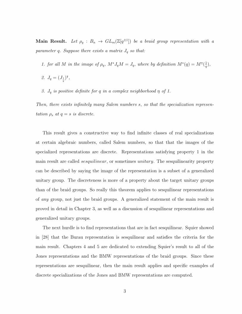
Main Result. Let ρq : Bn → GLm(Z[q±1]) be a braid group representation with a

parameter q. Suppose there exists a matrix Jq so that:

1. for all M in the image of ρq, M∗JqM = Jq, where by definition M∗(q) = Mᵀ(1

q),

2. Jq = (J 1q)ᵀ,

3. Jq is positive definite for q in a complex neighborhood η of 1.

Then, there exists infinitely many Salem numbers s, so that the specialization represen-

tation ρs at q = s is discrete.

This result gives a constructive way to find infinite classes of real specializations

at certain algebraic numbers, called Salem numbers, so that that the images of the

specialized representations are discrete. Representations satisfying property 1 in the

main result are called sesquilinear, or sometimes unitary. The sesquilinearity property

can be described by saying the image of the representation is a subset of a generalized

unitary group. The discreteness is more of a property about the target unitary groups

than of the braid groups. So really this theorem applies to sesquilinear representations

of any group, not just the braid groups. A generalized statement of the main result is

proved in detail in Chapter 3, as well as a discussion of sesquilinear representations and

generalized unitary groups.

The next hurdle is to find representations that are in fact sesquilinear. Squier showed

in [28] that the Burau representation is sesquilinear and satisfies the criteria for the

main result. Chapters 4 and 5 are dedicated to extending Squier’s result to all of the

Jones representations and the BMW representations of the braid groups. Since these

representations are sesquilinear, then the main result applies and specific examples of

discrete specializations of the Jones and BMW representations are computed.

3

Discreteness is an interesting structural property to study in light of the current

pursuit of thin groups and lattices. It turns out that the images of the braid group

representations in the main result are subgroups of lattices inside GLn(R). Chapter 6

explores the lattice structure and some commensurability results of the target lattices.

1.2 The Braid Groups

The braid groups are a very exciting and versatile mathematical object that are interest-

ing from an algebraic, geometric and topological point of view. The group presentation

given below was first introduced by E. Artin in 1925 [1].

Definition 1.2.1. The braid group on n strands, denoted Bn, is a group with the following

presentation:

Generators: σ1, · · · , σn−1

Relations: σiσj = σjσi for |i− j| > 1 (far commutativity)

σiσi+1σi = σi+1σiσi+1 for all i (braid relation)

From this algebraic perspective, we can easily see that this group is finitely generated,

finitely presented and infinite as each generator has infinite order. Also, the braid relation

can be rearranged

(σi+1σi)−1σi(σi+1σi) = σi+1

to show that the generators are conjugate. This is a particularly useful fact when studying

representations of the braid groups.

What is difficult to see from this algebraic definition is the motivation for the two

sets of relations. Viewing the braids from a more geometric perspective helps to see this

motivation.

Braids in Bn can be described as diagrams with n strands, which are stacks of the

generating diagrams σi and σ−1i defined in Figure 1.2.

4

1 i i+1 n

σi

1 i i+1 n

σ−1i

Figure 1.2: Generating diagrams for the braid group.

In σi, the strand in the i’th position crosses downwards behind the strand in the

i + 1 position, and in σ−1i the strand in the i’th position cross downwards in front of

the strand in the i + 1’th position. The braid group on n-strands is the collection of

diagrams created by stacking the σi’s, considered up to a certain isotopy of the strands.

Each braid can be described by listing the σi’s that occur in order from bottom to top.

The group multiplication is visualized by diagram stacking.

· =

σ1 σ2 σ1σ2

Figure 1.3: Multiplication is diagram stacking.

Importantly, what distinguishes a braid from a more general tangle is the monotonicity

of the strands, and the crossings occur at distinct heights in the braid. This is best seen

by orienting the strands with an upward flow. Braids are only considered up to isotopy

of the strands relative to the endpoints and which preserves the monotonicity of the

strands.

Example: The tangle in Figure 1.4 is not a braid because it can not be isotoped relative

the endpoints so that the strands flow monotonically upwards.

Example: The tangle in Figure 1.5 is a braid because it can be isotoped relative end-

points to the braid (σ−11 )3.

The far commutativity relation is easy to visualize with this geometric perspective.

5

Figure 1.4: A tangle that is not a braid.

=

Figure 1.5: A tangle that is a braid.

=

σ1σ3 σ3σ1

Figure 1.6: Far commutativity relation.

=

σ1σ2σ1 σ2σ1σ2

Figure 1.7: The braid relation.

6

If σi and σj use disjoint strands in their crossings, then there is an acceptable isotopy

that slides the crossings passed each other, as shown in Figure 1.6.

Knot theoretically, the braid relation is easy to see as a Reidemeister III move applied

to the strands. Or rather, the middle strand can slide in between the other two strands,

which changes the order of the crossings, as shown in Figure 1.7.

The braid relation shows that σi and σi+1 do not commute with each other, but rather

entangle with each other. Since the generators do not all commute, it is a bit surprising

is that the braid groups have a non trivial center.

Theorem 1.2.2 (van Buskirk [29]). The center of Bn is cyclic generated by

(σ1σ2 · · ·σn−1)n.

Using this visual description, it is easy to visualize that (σ1σ2 · · ·σn−1)n is central,

but difficult to see that it generates all of the center.

1.3 Where do the braid groups arise in real life?

E. Artin in 1925 [1] was the first person to name the braid groups and give an explicit

algebraic presentation for these groups. While this is the most famous introduction of

the braid groups, their existence and some deep properties were known far before 1925 in

the early descriptions of mapping class groups, by Hurwitz and Fricke-Klein in the late

1800’s though these references are difficult to find today.

This section briefly outlines several ways the braid groups arise in various different

mathematical settings.

Mapping Class Group

The mapping class group of a topological space M is the group of isotopy classes of

homeomorphisms of M . The braid group is the mapping class group of an n-punctured

7

disc where the homeomorphisms fix the boundary. This can be seen by visualizing each

puncture connected to the boundary by a string. After the homeomorphism is applied,

the punctures have swapped places and the strings are braided.

Fundamental group of configuration space

The configuration space of n points is defined to be

Cn = (x1, · · · , xn) ∈ Cn|xi 6= xj if i 6= j.

There is a natural action of the symmetric group Sn on Cn by permuting the coordi-

nates. Then Bn is the fundamental group of Cn modulo this action, Bn∼= π1(Cn)/Sn.

Knot Theory

A knot is a smooth embedding of the circle S1 into R3. A link is an embedding of multiple

circles. The knot type of a knot(or link) is the equivalence class of the knot up to ambient

isotopy. The major question in knot theory is to determine the knot type of a knot, or

tell when two knots are “the same” or “not the same”. Knots are often drawn as planar

projections with the crossings indicated by a gap in the under strand.

These projections are called knot diagrams. The same knot can have wildly different

diagrams, which are related by Reidemeister moves. Braids can serve as one way to

standardize these diagrams. Every braid gives rise to a knot or link by taking the braid

closure. The braid closure is formed by adding arcs that connect the i’th strand at the

top of the braid to the i’th strand at the bottom of the braid.

8

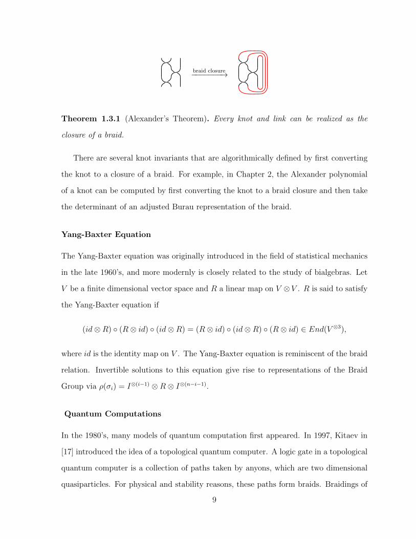
braid closure−−−−−−−→

Theorem 1.3.1 (Alexander’s Theorem). Every knot and link can be realized as the

closure of a braid.

There are several knot invariants that are algorithmically defined by first converting

the knot to a closure of a braid. For example, in Chapter 2, the Alexander polynomial

of a knot can be computed by first converting the knot to a braid closure and then take

the determinant of an adjusted Burau representation of the braid.

Yang-Baxter Equation

The Yang-Baxter equation was originally introduced in the field of statistical mechanics

in the late 1960’s, and more modernly is closely related to the study of bialgebras. Let

V be a finite dimensional vector space and R a linear map on V ⊗V . R is said to satisfy

the Yang-Baxter equation if

(id⊗R) (R⊗ id) (id⊗R) = (R⊗ id) (id⊗R) (R⊗ id) ∈ End(V ⊗3),

where id is the identity map on V . The Yang-Baxter equation is reminiscent of the braid

relation. Invertible solutions to this equation give rise to representations of the Braid

Group via ρ(σi) = I⊗(i−1) ⊗R⊗ I⊗(n−i−1).

Quantum Computations

In the 1980’s, many models of quantum computation first appeared. In 1997, Kitaev in

[17] introduced the idea of a topological quantum computer. A logic gate in a topological

quantum computer is a collection of paths taken by anyons, which are two dimensional

quasiparticles. For physical and stability reasons, these paths form braids. Braidings of

9

anyons in a topological quantum computer change the encoded quantum information,

giving rise to a quantum computation. So, representations of the braid groups can be

used to describe quantum computations. [10]

1.4 Representation Theory

This section will define the standard terminology of representation theory that will be

used throughout the thesis.

Definition 1.4.1. A representation of a group G is a group homomorphism ρ : G→

GL(V ) for some vector space V . A representation can also be defined in terms of a group

action or a module structure.

Definition 1.4.2. A representation is irreducible if it has no proper sub-representations.

(Under nice circumstances, this is equivalent to a representation which is not a direct sum

of representations.)

Definition 1.4.3. A representation is faithful if it is an injective homomorphism.

Definition 1.4.4. A representation is discrete if its image is a discrete subgroup of

GLm(R), with the standard euclidean topology.

Definition 1.4.5. A representation is parameterized by a variable t if the image

lies in GL(Z[t±1]).

Definition 1.4.6. For a parameterized representation ρ, a specialization of ρ at s ∈ C

is a composition of ρ and the evaluation map t = s.

1.4.1 Representations of the Braid Groups

As described in Section 1.3, the braid groups arise in several different mathematical

settings, many of which induce representations of the braid groups.

10

Representations of

the braid groups

Hecke & BMWalgebras

Monodromyactions of π1

Mapping classgroup actions

Solutions toYang-Baxter eq

knot

invariants

Thin

subgroups

Top.quantum

computing

The Jones representations and one of its irreducible summands, the Burau representa-

tion, are very well known representations and are described in detail in the later chapters.

These representations are very important for a myriad of reasons, but particularly for

the following two properties.

1. The Jones representations parameterize all of the irreducible representations of the

braid groups with two eigenvalues.

2. For n = 4, Bigelow conjectured and Tetsuya Ito proved that the faithfulness of the

Burau representation implies that the Jones polynomial detects the unknot [3,13].

More precisely, the Burau representation for n = 4 is unfaithful if and only if there

is a knot with braid index 4 and trivial Jones polynomial. It is known that the Jones

polynomial is not a complete knot invariant, but it is unknown whether it detects

the unknot. So deeper understanding the Burau representation can significantly

impact the field of knot theory.

The Jones representations are parameterized by a variable q, though for the Burau

representation the variable is typically denoted by a t. The main results in this thesis are

about choosing careful specializations of the parameter so that the image is a discrete

group.

11

1.5 Motivation For Discreteness

There are two major motivations for discrete representations: the search for thin groups,

and Wielenberg’s Theorem.

A lattice is a discrete subgroup of a Lie Group that has finite co-volume. A thin

group can be thought of as a generalization of a lattice. That is, a thin group is a

Zariski dense, infinite index subgroup of a lattice. One possible approach to find thin

groups is to first find discrete representations of a group into a lattice with infinite image.

The image is a subgroup of the lattice which has potential to be thin.

A second motivation is Wielenberg’s theorem stated below. This theorem gives a

way to create faithful representations using sequences of discrete representations. This

is particularly interesting in light of the open faithfulness question for the Burau repre-

sentation.

Theorem 1.5.1 (Wielenberg, [32]). Let ρi : Bn → G be a sequence of discrete represen-

tations, where G is a linear Lie Group. Suppose that

1. For each non trivial γ ∈ Bn, there exists Kγ so that for k > Kγ, ρk(γ) 6= IdG,

2. ρi converges algebraically to ρ : Bn → G,

then ρ is faithful, except possibly on the center of Bn

Here, converges algebraically means for each ω ∈ Bn, ρ(ω) = limi→∞ρi(ω).

Proof. This proof follows that of Kapovich [16]. Let K be the kernel of ρ. Since Bn is

torsion free, then K is torsion free.

Since G is a linear Lie Group, the nilpotency class of its subgroups is bounded above

by some constant c. Fix any finite collection g1, · · · , gk ∈ K. Suppose the subgroup

〈g1, · · · , gk〉 is not nilpotent of class c, then there exists some commutator word of length

c, ω := [x1, [x2, [. . . ] . . . ] 6= 1, for xi ∈ 〈g1, · · · , gk〉.

12

Choosing sufficiently large i, ρi(ω) 6= IdG, and for each gj, ρi(gj) 6= IdG and ρi(gj)

belongs to the Zassenhaus neighborhood of the identity in G. (A Zassenhaus neighbor-

hood is an open neighborhood Ω of the identity so that every discrete subgroup ∆ in

G which is generated by ∆ ∩ Ω is contained in a connected nilpotent Lie-subgroup of

G.) Since ρi is discrete, then 〈ρi(g1), · · · ρi(gk)〉 is discrete and generated by elements

in the Zassenhaus neighborhood, so the group 〈ρi(g1), · · · , ρi(gk)〉 is nilpotent of class c.

Since ρi(ω) is a commutator word of length c in 〈ρi(g1), · · · , ρi(gk)〉, then ρi(ω) = IdG

contradicting the choice of i.

Similarly, suppose K is not nilpotent of class c. Then there exists some braids

g1, ·, gk ∈ K and some commutator word ω′ of length c so that ω′(g1, · · · , gk) 6= 1. How-

ever, the group 〈g1, · · · , gk〉 is nilpotent of length c, so it must be that ω′(g1, · · · , gk) = 1.

Therefore K is nilpotent.

Thus, K is a normal, nilpotent subgroup of Bn, so K must be trivial or central.

13

Chapter 2

The Burau Representation

The Burau representation was first discovered by Werner Burau in 1935 [8]. This repre-

sentation has garnered much attention over the years for its question of faithfulness. It

is well known that the reduced Burau representation is faithful for n ≤ 3 and unfaithful

for n ≥ 5, but unknown for n = 4 [2,20,22].

Notation: There are two versions of the Burau representation: reduced and unreduced.

The reduced Burau representation is irreducible, while the unreduced is not. For the

remainder of this paper, the Burau representation is assumed to be reduced unless oth-

erwise specified.

In addition to its faithfulness intrigue, the Burau representation can also be used to

compute the Alexander polynomial of a knot [9,14]. If a knot K is the closure of a braid

ω in Bn, and ρ the Burau representation of Bn, then the Alexander polynomial ∆K(t) is

∆K(t) =1− t1− tn

det(Id− ρ(ω)).

2.1 Definition and Properties

Definition 2.1.1. The (reduced) Burau representation ρn : Bn → GLn−1(Z[t±1]) is given

by

14

σ1 7→

−t 1 00 1 00 0 Idn−3

, σn−1 7→

In−3 0 00 1 00 t −t

σi 7→

Idi−2 0 0 0 0

0 1 0 0 00 t −t 1 00 0 0 1 00 0 0 0 Idn−i−2

for 2 ≤ 1 ≤ n− 2

Squier showed in [28] that there exists a nonsingular n − 1 × n − 1 matrix J over

Z[t±1] so that for every w in Bn,

ρn(w)∗Jρn(w) = J.

Notation: For M ∈ GLn−1(Z[t±1]), the entries of M are integral polynomials in t and 1t,

and we denote M = M(t) and M(1t) to be the matrix that replaces t by 1

tin the entries

of M(t). The involution ∗ is given by M(t)∗ = M(1t)T .

Definition 2.1.2. A specialization of the Burau representation is a composition

representation τ ρn, where τ : GLn+1(Z[t±1]) → GLn+1(R) is an evaluation map de-

termined by t 7→ r for some fixed r ∈ R. Typically ρn is written at ρn,t viewing t as a

parameter, and the specialization is denoted ρn,r.

Theorem 2.1.3. For r ∈ C, the image of the specialization of the Burau representation

at r is isomorphic to the image when specializing to 1r. In particular, specializing to r is

discrete (faithful) if and only if specializing to 1r

is discrete (faithful).

Proof. Let ψ be the contragradient representation of ρn. For w ∈ Bn, if ρn(w) = M(t)

then ψ(w) = (M(t)−1)T where M ∈ GLn−1(Z[t±1]). From Squier, there exists a matrix

J so that

M(t)∗ = JM(t)−1J−1.

Taking the transpose of both sides shows that M(1t) is conjugate to (M(t)−1)T by JT .

15

Thus ρn and ψ are conjugate representations. Discreteness and faithfulness is preserved

by conjugation, inversion and transposition.

2.1.1 Details on Squier’s Form

As shown in Theorem 2.1.3, Squier’s form is a useful tool for proving structural results

about the image of the Burau representation. This section will give detailed computation

proofs for the following two results, which are necessary for later use. Letting J denote

Squier’s form,

1. In dimension n ≥ 4, det J = (1 + t)n (tn+1−1)(tn(t−1)) .

2. In dimension n, J may be chosen so it is positive definite for complex values of

t = eiθ for |θ| < 2πn+1

.

For notational clarity and in this section only, since the following arguments rely

heavily on the parameter t, Jt will be used to denote J .

Remark 2.1.4. Jt is hermitian when t is real or on the unit circle.

The following computations provide a change of basis to diagonalize Jt into a format

useful for analyzing its signature.

Let ei’s be the standard basis vectors in Cn and Ki = 1+t+···+ti−2

1+t+···+ti−1 . Define a new basis

for Cn as follows

v1 = 1

1 + t, 1, 0, · · · , 0

v2 = e1

v3 = e3 +K3v1

vi = ei +Kivi−1 for 3 < i ≤ n

16

Proposition 2.1.5. Let S be the matrix whose columns are the vj’s. Then −S∗JtS is a

diagonal matrix with k’th entry equal to (1+t)(tk+1−1)t(tk−1) for k ≥ 3 and first two entries equal

to −1+t+t2

tand − (1+t)2

t.

This proposition follows from the following computational claims.

Definition 2.1.6. 〈x, y〉Jt = x∗Jty is an antilinear form on C.

Claim 2.1.7. 〈vi, vj〉Jt = 0 for i 6= j.

Proof. 〈v1, v2〉Jt = v∗1Jtv2 = 11+ 1

t

b+ a = t1+t

(−2− t− 1t) + 1 + t = 0

Since vi = ei +Kivi−1, it suffices to prove that 〈vi, vi−1〉Jt = 0 for 1 ≥ 3.

〈v2, v3〉Jt = v∗2Jtv3 = e1Jt(e3 +K3v1) = e1Jte3 +K3e1Jtv1 = b, c, 0e3 +K3(b1t+1

+ c)

= K3(− (t−1)2t

1t+1

+ t+1t

)

Claim 2.1.8. 〈v1, v1〉Jt = −1+t+t2

tand 〈v2, v2〉Jt = − (1+t)2

t.

Proof. 〈v1, v1〉Jt = v∗1Jtv1 = [b t1+t

+ a, c t1+t

+ b, c, 0, · · · , 0]v1 = b t1+t

11+t

+ a 11+t

+ c t1+t

+ b

= − (t+1)2

tt

(1+t)2+ 1 + 1− (t+1)2

t= t−(1+t)2

t= −1+t+t2

t.

〈v2, v2〉Jt = v∗2Jtv2 = [b, c, 0, · · · , 0]v2 = b = − (1+t)2

t.

Claim 2.1.9. 〈vk, vk〉Jt = −(1+t)(tk+1−1)t(tk−1) = −(1+t)

tK−1k+1, for k ≥ 3.

Proof.

〈vk, vk〉Jt = v∗kJtvk = (K∗kvk−1 + e∗k)Jt(Kkvk−1 + ek)

= K∗kv∗k−1JtKkVk−1 +K∗kv

∗k−1Jtek + e∗kJtKkvk−1 + e∗kJtek

= KkK∗k(v∗k−1Jtvk−1) +K∗kv

∗k−1(0, · · · , 0, c, b) +Kk(0, · · · , 0, a, b)vk−1 + b

= KkK∗k(v∗k−1Jvk−1) +K∗kc+Kka+ b (∗)

Now Kk = 1+t+···+tk−2

1+t+···+tk−1 = tk−1−1tk−1 and so K∗k = t(tk−1−1)

tk−1 = tKk. Also, by inductive

hypothesis

v∗k−1Jtvk−1 = −(1+t)t

K−1k .

17

Thus from (∗) we get

〈vk, vk〉Jt = KkK∗k(−t−1(1− t)K−1k ) + tKkc+ kna+ b

= −(1 + t)Kk + tKk1 + t

t+Kka+ b

= Kka+ b

=tk−1 − 1

tk − 1(1 + t)− (1 + t)2

t

=(1 + t)(t(tk−1 − 1)− (1 + t)(tk − 1))

t(tk+1 − 1)

= −(1 + t)(tk+1 − 1)

t(tk − 1)=−(1 + t)

tK−1k+1

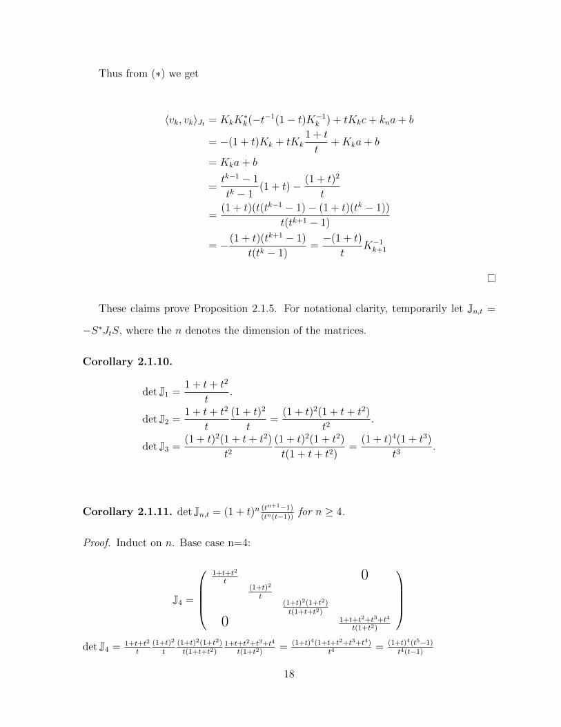
These claims prove Proposition 2.1.5. For notational clarity, temporarily let Jn,t =

−S∗JtS, where the n denotes the dimension of the matrices.

Corollary 2.1.10.

det J1 =1 + t+ t2

t.

det J2 =1 + t+ t2

t

(1 + t)2

t=

(1 + t)2(1 + t+ t2)

t2.

det J3 =(1 + t)2(1 + t+ t2)

t2(1 + t)2(1 + t2)

t(1 + t+ t2)=

(1 + t)4(1 + t3)

t3.

Corollary 2.1.11. det Jn,t = (1 + t)n (tn+1−1)(tn(t−1)) for n ≥ 4.

Proof. Induct on n. Base case n=4:

J4 =

1+t+t2

t0

(1+t)2

t(1+t)2(1+t2)t(1+t+t2)

0 1+t+t2+t3+t4

t(1+t2)

det J4 = 1+t+t2

t(1+t)2

t(1+t)2(1+t2)t(1+t+t2)

1+t+t2+t3+t4

t(1+t2)= (1+t)4(1+t+t2+t3+t4)

t4= (1+t)4(t5−1)

t4(t−1)

18

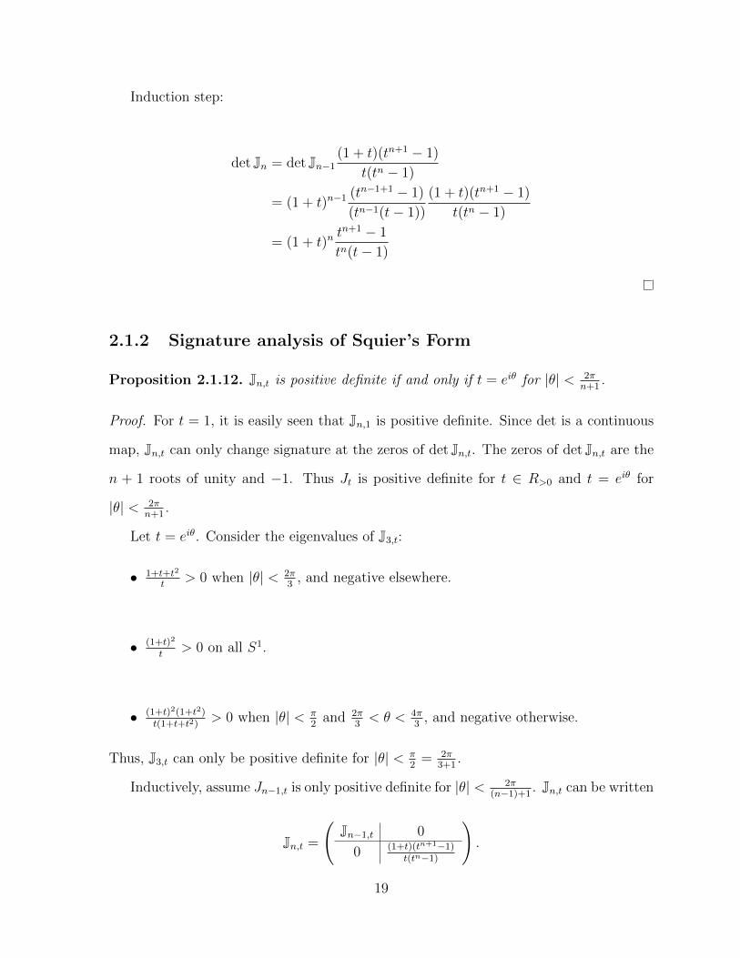
Induction step:

det Jn = det Jn−1(1 + t)(tn+1 − 1)

t(tn − 1)

= (1 + t)n−1(tn−1+1 − 1)

(tn−1(t− 1))

(1 + t)(tn+1 − 1)

t(tn − 1)

= (1 + t)ntn+1 − 1

tn(t− 1)

2.1.2 Signature analysis of Squier’s Form

Proposition 2.1.12. Jn,t is positive definite if and only if t = eiθ for |θ| < 2πn+1

.

Proof. For t = 1, it is easily seen that Jn,1 is positive definite. Since det is a continuous

map, Jn,t can only change signature at the zeros of det Jn,t. The zeros of det Jn,t are the

n + 1 roots of unity and −1. Thus Jt is positive definite for t ∈ R>0 and t = eiθ for

|θ| < 2πn+1

.

Let t = eiθ. Consider the eigenvalues of J3,t:

• 1+t+t2

t> 0 when |θ| < 2π

3, and negative elsewhere.

• (1+t)2

t> 0 on all S1.

• (1+t)2(1+t2)t(1+t+t2)

> 0 when |θ| < π2

and 2π3< θ < 4π

3, and negative otherwise.

Thus, J3,t can only be positive definite for |θ| < π2

= 2π3+1

.

Inductively, assume Jn−1,t is only positive definite for |θ| < 2π(n−1)+1

. Jn,t can be written

Jn,t =

(Jn−1,t 0

0 (1+t)(tn+1−1)t(tn−1)

).

19

Within the constraint that |θ| < 2π(n−1)+1

, the last eigenvalue (1+t)(tn+1−1)t(tn−1) is only posi-

tive when |θ| < 2πn+1

. Thus Jn,t is only positive definite for |θ| < 2πn+1

.

Moreover, since each eigenvalue has at most one repeated root (at -1), each eigenvalue

alternates sign around the circle changing at roots of unity. Thus the signature of Jn,t

starts at (n, 0) at t = 1 and changes incrementally to (0, n) at(near) t = −1.

Remark 2.1.13. If α is a positive real number, then αJn,t is also positive definite if and

only if t ∈ R>0 or t = eiθ for |θ| < 2πn+1

.

2.2 Details on the Burau Representation of B3

The goal of this Section is to prove a complete classification of the real discrete special-

izations of the Burau representation of B3 described in the following theorem.

Theorem 2.2.1. The real discrete specializations of the Burau representation of B3 are

exactly when t satisfies one of the following:

1. t < 0 and t 6= −1

2. 0 < t ≤ 3−√5

2or t ≥ 3+

√5

2

3. 3−√5

2< t < 3+

√5



2.2.1 Subgroup Properties of B3

There are two well known subgroups of B3 that play a vital role in the classification.

1. The center of B3 is Z(B3) = 〈(σ1σ2)3〉 which is cyclic.

20

2. The normal subgroup N = 〈a1, a2〉 where a1 = σ−11 σ2 and a2 = σ2σ−11 , which is a

free group on two generators. A proof of this will be shown in the proof of Theorem

2.2.1.

These subgroups will be used in combination with the following Lemmas and Theorem.

Lemma 2.2.2 (Long [21]). Let ρ : Bn → GL(V ) be a representation and K / Bn with

K nontrivial and non central. If ρ|K is faithful, then ρ is faithful except possibly on the

center.

Lemma 2.2.3. Every homomorphism φ on N with φ(N) a free group of rank two is an

isomorphism onto its image.

Proof. Since N is a free group of rank two, it is Hopfian. It is given that φ(N) is also a

free group of rank two. Therefore by definition of Hopfian, φ must be an isomorphism

on N .

Definition 2.2.4. The Burau representation of B3 is the homomorphism ρ3 : B3 →

GL2(Z[t, t−1]) given by

ρ3(σ1) =

(−t 10 1

)and ρ3(σ2) =

(1 0t −t

).

Lemma 2.2.5. The Burau representation of B3 is faithful on the center for all real

specializations of t except t = 0,±1.

Proof. The center of B3 is cyclicly generated by (σ1σ2)3, where

ρ3((σ1σ2)

3)

=

(t3 00 t3

).

This shows that ρ3(Z(B3)) is a free group on one generator when t 6= ±1, 0. So ρ3 is

faithful on Z(B3).

21

Corollary 2.2.6. Away from 0 and ±1, if a specialization the Burau representation is

faithful on N , then it is faithful on all of B3.

Proof. Lemma 2.7 proves that the specialization is faithful on the center. Since N is a

normal subgroup of B3, Lemma 2.5 guarantees that the specialization is faithful on the

rest of B3.

Theorem 2.2.7. If ρ3 is discrete on N , then ρ3 is discrete on all of B3.

Proof. Assume for a contradiction that γk is a sequence in ρ3(B3) converging to the

identity but γk 6= Id for all k. Then for every fixed φ ∈ ρ3(N), the commutator sequence

[φ, γk] also converges to the identity. Since N is normal and ρ3(N) is discrete, then

[φ, γk] ⊆ ρ3(N) and for some n0 ∈ N, [φ, γk] = Id for all k > k0. This gives that for all

k > n0,

φγk = γkφ.

This shows that every φ ∈ ρ3(N) commutes with γk for large k, and further φ and γk

have the same fixed points. Because B3 is not virtually solvable, ρ3(B3) is non-elementary

and ρ3|N is discrete, there exists two hyperbolic element η and φ of ρ3(N) so that φ and

η have different fixed points [26, p. 606]. This contradicts the fact that both φ and η

must have the same fixed points as γk for large enough k.

Remark: Theorem 2.2.7 can be generalized with effectively the same proof, but is a

slight tangent from the realm of braids and requires a bit of hyperbolic geometry.

Theorem 2.2.7 generalized: Let G be a group that is not virtually solvable and K a

non central normal subgroup of G. If ρ : G → Isom+(Hn) is a homomorphism so that

ρ(G) is non-elementary, ρ|K is discrete, and ρ(K) 6⊂ Ker(ρ) then ρ is discrete on all of

G.

22

2.3 Complete Classification of the Real Discrete Spe-

cializations of the Burau Representation of B3

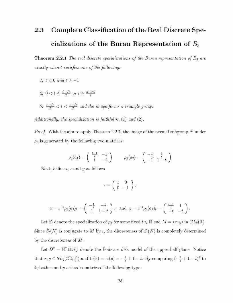
Theorem 2.2.1 The real discrete specializations of the Burau representation of B3 are

exactly when t satisfies one of the following:

1. t < 0 and t 6= −1

2. 0 < t ≤ 3−√5

2or t ≥ 3+

√5

2

3. 3−√5

2< t < 3+

√5



Proof. With the aim to apply Theorem 2.2.7, the image of the normal subgroup N under

ρ3 is generated by the following two matrices.

ρ3(a1) =

(t−1t−1

t −t

)ρ3(a2) =

(−1

t1t

−1 1− t

)Next, define ι, x and y as follows

ι =

(1 00 −1

),

x = ι−1ρ3(a2)ι =

(−1

t−1

t

1 1− t

), and y = ι−1ρ3(a1)ι =

(t−1t

1−t −t

).

Let St denote the specialization of ρ3 for some fixed t ∈ R and M = 〈x, y〉 in GL2(R).

Since St(N) is conjugate to M by ι, the discreteness of St(N) is completely determined

by the discreteness of M .

Let D2 = H2 ∪ S1∞ denote the Poincare disk model of the upper half plane. Notice

that x, y ∈ SL2(Z[t, 1t]) and tr(x) = tr(y) = −1

t+ 1− t. By comparing (−1

t+ 1− t)2 to

4, both x and y act as isometries of the following type:

23

1. Hyperbolic when t < 0 or 0 < t < 3−√5

2or t > 3+

√5

2,

2. Elliptic when 3−√5

2< t < 3+

√5

2,

3. Parabolic when t = 3±√5

2.

Consider the following cases on t ∈ R.

Case 1) Let t < 0.

In this range of t, both x and y act as hyperbolic isometries on D2. Consider the following

images of ∞:

y−1(∞) = −1, and xy−1(∞) = 0

yxy−1(∞) = −1

t= x(∞).

The shaded region of Figure 2.1 is a fundamental domain for the action of M on D2.

So H2/M is a punctured torus, showing that M and St(N) are discrete, and M is a free

group of rank 2. By Theorem 2.2.7, since St is discrete on N then it is discrete on all of

B3.

p

xyx−1(∞) = 1−t = x(∞)∞

y−1(∞) = −1 xy−1(∞) = 0

A

B

C

D

Figure 2.1: D2 with geodesics connecting images of ∞, when t < 0.

To see why the action is discrete, it suffices to show that the center point p can never

be fixed by an element of M . Let A,B,C and D be the un-shaded regions in the disk

bounded by the geodesics as shown in Figure 2.1. Notice that x(p) ∈ B, x−1(p) ∈ D,

y(p) ∈ A and y−1(p) ∈ C. Similarly, for any integer n, xn(p) ∈ D∪B and yn(p) ∈ A∪C.

Lastly, xn(A ∪ C) ⊂ D ∪ B and yn(D ∪ B) ⊂ A ∪ C. Any element in M is of the form

24

xe1ye2 · · ·xem−1yem for some ei ∈ Z, giving that xe1ye2 · · ·xem−1yem(p) ∈ A ∪ B ∪ C ∪ D

and could not possibly fix p.

Case 2) Let t = 3+√5

2.

For this value of t, x, y and yx−1 are parabolic isometrics. Let x−1f , yf and zf denote

fixed points of x−1, y and yx−1 respectively. By computing eigenvectors, these fixed

points are

x−1f =−1 +

√5

2, yf =

1−√

5

2, zf =

−7 + 3√

5

2.

Figure 2.2 shows a fundamental domain for the action of M on D2, showing that

H2/M is a thrice punctured sphere. By the same arguments as in case 1, St is discrete

and faithful on all of B3.

zf

x−1(zf )

yfx−1f

Figure 2.2: The shaded region is the fundamental domain for the action of M on D2

when t = 3+√5

2.

Case 3) Let t > 3+√5

2.

In this region, both x, y, yx and yx−1 act as hyperbolic isometries on the D2. As

shown in Case 2, the fixed points of x−1, y and yx−1 are distinct when t = 3+√5

2. If there

exists a t so that any two of x−1, y or x−1y shared a fixed point then, then both x−1

and y share a fixed point. In other words, x−1 and y have a common eigenvector and are

25

simultaneously conjugate to matrices of the form

x−1 ∼(a ∗0 a−1

)and y ∼

(b ∗0 b−1

)for some a, b ∈ R. This forces the commutator [x−1, y] to have the form

[x−1, y] ∼(

1 ∗0 1

),

which gives tr([x−1, y]) = 2. However, by direct computation, tr([x−1, y]) = (1+t2)(1−t2+t4)t3

which is strictly greater than 2 for t > 3+√5

2. So as t increases, all six fixed points of x−1,

y and x−1y remain distinct for all t > 3+√5

2.

Let x±, and y± denote the fixed points of each x, y respectively. Since x, y, yx, and

yx−1 are all hyperbolic in this interval for t, there exists disjoint geodesics about each of

x± and y± as shown in Figure 2.3. The action of M on D2 shows that H2/M is a pair of

pants, and thus St is discrete and faithful on B3.

x+

y+

x−y−

Figure 2.3: The shaded region is the fundamental domain for the action of M on D2

when t > 3+√5

2.

Case 4) Let 0 < t ≤ 3−√5

2.

Immediately from case 2, case 3, and Theorem 2.2.7, St is discrete and faithful on all

of B3.

26

Case 5) Let 3−√5

2< t < 3+

√5

2.

In this region, x−1, y and yx−1 are all elliptic with the same trace 1− t− 1t. Elliptic

isometries are diagolizable with diagonal entries complex conjugate roots of unity. So

the trace is 2 cos θ for some θ which is the rotation angle for the isometry. At t = 3+√5

2,

the trace of x−1, y and yx−1 are all equal to −2. To account for this negative sign, the

following equation must hold

−2 cos θ = 1− t− 1

t.

Solving for t in terms of θ gives

t =1 + 2 cos θ ±

√(2 cos θ + 1)2 − 4

2.

Since t is real valued, the discriminant must be nonnegative, forcing

cos θ ≤ −3

2or cos θ ≥ 1

2.

Thus, the only possible rotation angles for x−1, y and yx−1 are 0 ≤ θ ≤ π3

or 5π3≤ θ ≤ 2π.

Consider the following cases for θ.

1. If θ = dπ where d is irrational.

Let xf and yf be the fixed points of x and y respectively. Since y acts as a rotation

about yf , the set yi(xf )i∈N lies in an S1 centered at yf . Since θπ

is irrational,

yi(xf ) is distinct for each i. By compactness, yi(xf )i∈N has an accumulation

point, giving the orbit of xf is not discrete and the action of M is not discrete.

2. If θ = 2πn

for some n ∈ Z.

Then M is the triangle group with presentation 〈x, y|xn = yn = (xy)n = 1〉. The

bounds for θ force n ≥ 6 and all such n occur from specializations of t satisfying

3−√5

2< t < 3+

√5

2. For n ≥ 6, 1

n+ 1

n+ 1

n< 1 so M is a hyperbolic triangle group

and is known to be discrete.

27

3. If θ = 2πkm

for k,m ∈ Z relatively prime.

The classification of good orbifolds gives that D2/M can not yield a cone angle of

2πkm

for k,m ∈ Z relatively prime. So the action of M is not discrete.

2.4 Corollaries and Examples

There is interesting faithfulness interplay between the Burau representations ρ3 on B3

and ρ4 on B4. The underlying reason for this interplay is the block structure of ρ4 shown

in the definition below.

ρ4(σ1) =

−t 1 00 1 00 0 1

=

ρ3(σ1)0

00 0 1

,

ρ4(σ2) =

1 0 0t −t 10 0 1

=

ρ3(σ2)0

10 0 1

,

ρ4(σ3) =

1 0 00 1 00 t −t

.

One way to create an unfaithful specialization of ρ4 is to “extend” an unfaithful

specialization of ρ3. More precisely, suppose the specialization of ρ3 at η is unfaithful, and

let K denote the kernel in B3. We can identify K as a subgroup of B4 under the standard

inclusion. From the block structures shown above, ρ4(K) consists of upper triangular

matrices with ones along the diagonals, which is a nilpotent group as a subgroup of the

Heisenberg group. Thus the upper central series finitely terminates yielding a nontrivial

subgroup of K that maps to the identity by ρ4. Therefore, the specialization of ρ4 at η

is also unfaithful.

28

Example 4.1 shows one method to create unfaithful specializations of ρ3, which con-

sequently are also unfaithful specializations of ρ4. Because of this consequential relation-

ship, it is perhaps more interesting to find an unfaithful specialization of ρ4 that is faithful

when restricted to B3. Example 2.4.1 gives a construction of such a specialization.

Example 2.4.1. A method to create unfaithful specializations of ρ3 on B3.

Let w be a word in B3 different from σk1 . Let fw be a polynomial factor of the 2-1 entry

of ρ3(w) and tw be a root of fw. Specializing to t = tw leaves Stw(w) an upper triangular

matrix. Since the image of σ1 is also upper triangular, the group 〈Stw(σ1), Stw(w)〉 is

solvable. Therefore, specializing to tw cannot be faithful since B3 does not have solvable

subgroups.

Some examples such w’s and fw’s are listed here.

1. Let w = σ−22 σ1σ−12 with fw = −1 + t− 2t2 + t3 which has one real root.

2. Let w = σ52σ

21σ−42 σ1σ

32 and

fw = 1− 3t+ 6t2 − 10t3 + 13t4 − 16t5 + 16t6 − 15t7 + 12t8 − 8t9 + 5t10 − 3t11 + t12

which has two real roots.

Theorem 2.2.1 proved that all real unfaithful specializations of ρ3 come from the

interval (3−√5

2, 3+

√5

2). Thus we can conclude that all real roots of fw must lie in the

interval (3−√5

2, 3+

√5

2). This proves the following corollary.

Corollary 2.4.2. Real roots of the 2-1 entries of Burau matrices not in 〈σ1〉 must lie in

the interval (3−√5

2, 3+

√5

2).

Example 2.4.3. An unfaithful specialization of ρ4 on B4.

For simplification, let x = σ1σ−13 and y = σ2xσ

−12 . Consider the following words

ω1 = x−1y2x−1yxyx2y−2x−1y−3 (2.1)

ω2 = y−1xy−2xy−1x−1y−1x−2y2xy2. (2.2)

29

One can check that ρ4(ω1) 6= ρ4(ω2). However, for St0 the specialization of ρ4 to

t0 = 3+√5

2, the equality St0(ω1) = St0(ω2) occurs. Theorem 2.2.1 proved that specializing

ρ3 at t0 is faithful. Thus, the infidelity of ρ4 at t0 is truly a property of B4, not a conse-

quence of containing B3.

2.4.1 Moving forward from B3

Keeping inline with the previous discussions of discreteness, Squier’s form easily gives

the next result.

Proposition 2.4.4. The image of the specialization of the Burau representation is dis-

crete at real quadratic algebraic units with positive norm.

Proof. Let α be a real quadratic algebraic unit with positive norm and σ be the generator

of the Galois group of Q(α). The map σ is determined by σ(α) = α−1, since α has positive

norm. Fix arbitrary n and consider the Burau representation on Bn specialized at α, and

J the associated Squier’s form. Let Ak be a sequence of matrices in the image of this

specialization and assume that Ak converges to the Id. Each Ak has entries in Q(α),

so the defining relation of Squier’s form A∗kJAk = J becomes (Aσk)T = JA−1k J−1. So if

Ak → Id then so does Aσk . Since σ is the only field automorphism, the entires (Ak)ij are

all algebraic integers of bounded absolute value and degree. There are only finitely many

such algebraic integers, so the entries (Ak)ij must be eventually constant.

Corollary 2.4.5. The specialization of the Burau representation of B3 at 3+√5

2is discrete.

The number 3+√5

2is particularly interesting as ρ3 specialized at 3+

√5

2is both discrete

and faithful, while specializing ρ4 at 3+√5

2is discrete and yet unfaithful.

The discreteness in Theorem 2.2.1 required specific characteristics of B3 and the fact

that the Burau representation is 2-dimensional. However, Proposition 2.4.4 only required

30

Squier’s form and no limitations of the dimension of the representation. Proposition

2.4.4 is motivation for a larger class of discrete representations using Salem numbers and

generalized unitary groups, which will be described in the next chapters.

31

Chapter 3

Discrete Generalized Unitary

Groups

3.1 Generalized Unitary Groups

A matrix is unitary over the complex numbers if MᵀM = Id, where M is the complex

conjugate of M . We can rewrite this as Mᵀ · Id ·M = Id. The collection of all unitary

matrices over C gives the unitary group, denoted

U(Id,−,C) =: M ∈ GL(C)|Mᵀ · Id ·M = Id.

We can generalize this group to use an arbitrary coefficient ring R, and an order two

automorphism φ of R.

U(Id, φ,R) =: M ∈ GL(R)|φ(M)ᵀ · Id ·M = Id

When the automorphism φ is understood, we will denote M∗ = φ(M)ᵀ. To generalize

further, if J is a matrix satisfying J∗ = J , then we can get

U(J, φ,R) =: M ∈ GL(R)|M∗JM = J.

32

Definition 3.1.1. U(J, φ,R) =: M ∈ GL(R)|M∗JM = J is called the generalized

unitary group, where M∗ = φ(M)ᵀ and J∗ = J .

Here J is called a sesquilinear form and if a representation has image in such a

generalized unitary group, it is called a sesquilinear representation. This generalized

unitary group can be thought of as the collection of matrices that preserve an inner

product given by

〈v, w〉 = v∗Jw.

Example 3.1.2. Let R = Q(√

5) and φ be the field automorphism defined by√

5 7→ −√

5.

For J and X below, X ∈ U2(J, φ,Q(√

5)).

J =

(−10 5 +

√5

5−√

5 10

)X =

(−3+

√5

21

0 1

)Example 3.1.3. How does this apply to the Burau representations? Squier showed that

the Burau representations are sesquilinear with respect to Squier’s form J . Letting φ be

the involution given by t 7→ 1t, we can write

ρn : Bn+1 → Un(J, φ,Z[t±1]).

3.2 Discrete Generalized Unitary Groups

Discreteness of a unitary group is a balance between the form J and the choice of coeffi-

cient ring.

Example 3.2.1. Proposition 2.4.4 can be restated as follows: For α a real quadratic

algebraic unit with positive norm, OQ(α) the ring of integers for Q(α), φ the map that

sends α 7→ 1α

, and J a nondegenerate form over Fix(φ), then the generalized unitary

group Um(J, φ,OQ(α)) is discrete.

This example of discreteness can be extended to a larger class of number rings with

greater than quadratic dimension. Let L be a totally real algebraic field extension of

33

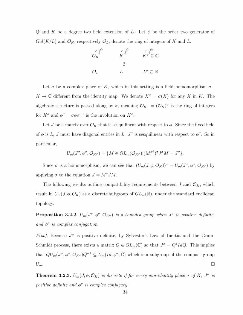
Q and K be a degree two field extension of L. Let φ be the order two generator of

Gal(K/L) and OK , respectively OL, denote the ring of integers of K and L.

K

L

2

φ

OK

OL

φ

Kσ ⊆ C

Lσ ⊆ R

φσ

Let σ be a complex place of K, which in this setting is a field homomorphism σ :

K → C different from the identity map. We denote Xσ = σ(X) for any X in K. The

algebraic structure is passed along by σ, meaning OKσ = (OK)σ is the ring of integers

for Kσ and φσ = σφσ−1 is the involution on Kσ.

Let J be a matrix over OK that is sesquilinear with respect to φ. Since the fixed field

of φ is L, J must have diagonal entries in L. Jσ is sesquilinear with respect to φσ. So in

particular,

Um(Jσ, φσ,OKσ) = M ∈ GLm(OKσ)|(Mφσ)ᵀJσM = Jσ.

Since σ is a homomorphism, we can see that (Um(J, φ,OK))σ = Um(Jσ, φσ,OKσ) by

applying σ to the equation J = M∗JM .

The following results outline compatibility requirements between J and OK , which

result in Um(J, φ,OK) as a discrete subgroup of GLm(R), under the standard euclidean

topology.

Proposition 3.2.2. Um(Jσ, φσ,OKσ) is a bounded group when Jσ is positive definite,

and φσ is complex conjugation.

Proof. Because Jσ is positive definite, by Sylvester’s Law of Inertia and the Gram-

Schmidt process, there exists a matrix Q ∈ GLm(C) so that Jσ = Q∗IdQ. This implies

that QUm(Jσ, φσ,OKσ)Q−1 ⊆ Um(Id, φσ,C) which is a subgroup of the compact group

Um.

Theorem 3.2.3. Um(J, φ,OK) is discrete if for every non-identity place σ of K, Jσ is

positive definite and φσ is complex conjugacy.

34

Proof. Assume that Mn converges to the identity in Um(J, φ,OK). To show Mn is

eventually constant, we will show that for n large, there are only finitely many possibilities

for the entries (Mn)ij.

By assumption, for each σ the group Um(Jσ, φσ, OKσ) is bounded by Proposition

3.2.2. Also, for every Mn, Mσn ∈ Um(Jσ, φσ, OKσ). So there exists a B so that for large

n, for all i, j, and for all σ, that |(Mσn )ij| < B.

For everyM ∈ Um(J, φ,OK), the equationM∗JM = J can be rearranged to JMJ−1 =

((Mφ)ᵀ)−1, showing that M and ((Mφ)ᵀ)−1 are simultaneously conjugate. Thus Mφn

also converges to the identity. Convergent sequences are bounded, so for large enough n,

|(Mn)ij| < B and |(Mn)φij| < B for every ij-entry.

L is a totally real degree two subfield of K, and φ generates Gal(K/L). So K has

one non-identity real embedding φ, and all other embeddings are complex. Thus we have

shown above that for large n there is a uniform bound B for each entry (Mn)ij and each

Galois conjugate of (Mn)ij. There are only finitely many algebraic integers α so that

deg(α) ≤ deg(K/Q), and with the property that α and all of the Galois conjugates of α

have absolute value bounded above by B. So there are only finitely many possible entries

for (Mn)ij, which implies the sequence Mn is eventually constant.

Corollary 3.2.4. If ρ : G → Um(J, φ,OK) is a representation of a group G so that for

every non-identity place σ of K, Jσ is positive definite and φσ is complex conjugacy, then

ρ is a discrete representation.

With the Burau representation in mind, Theorem 3.2.3 requires an algebraic unit α

so that Squier’s form J is positive definite at all of the non-identity embeddings of α, in

addition to properties of the number ring of α. Recall from Proposition 2.1.12 that J is

positive definite in a neighborhood of 1 on the unit circle. This need motivates the use

of Salem numbers in the next section.

At first glance, the requirements for Corollary 3.2.4 seem very specific and perhaps it

is doubtful that any such a representation could exist. However, as described in section

35

2.1, Squier showed that the Burau representation maps into a generalized unitary group

over Z[t, t−1], so the next task is to find values of t so that so the form and coefficient

ring satisfy the specific hypothesis of Corollary 3.2.4. Section 3.4 will show how careful

specializations of t to certain Salem numbers meet all of the conditions for Corollary

3.2.4. More generally, Section 4.0.1 will show that every irreducible Jones representation

fixes a form Jt with a parameter, and specializations to Salem numbers can also be found

to satisfy Corollary 3.2.4.

3.3 Salem Numbers

Salem numbers are the key ingredient to the application of Corollary 3.2.4, which requires

a real algebraic number field with tight control and understanding of each of its complex

embeddings.

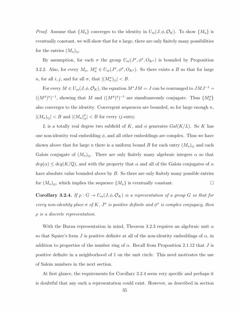
Definition 3.3.1. A Salem number s is a real algebraic unit greater than 1, with one

real Galois conjugate 1s, and all complex Galois conjugates have absolute value equal to

1.

s

For example, the largest real root of Lehmer’s Polynomial, called Lehmer’s number,

x10 + x9 − x7 − x6 − x5 − x4 − x3 + x+ 1,

is a Salem number. Trivial Salem numbers of degree two are solutions to s2 − ns+ 1 for

n ∈ N, n > 2.It is well known that there are infinitely many Salem numbers of arbitrarily

large absolute value and degree. In particular, if s is a Salem number, then sm is also a

Salem number for every positive integer m. One geometric consequence of this property

that powers of Salem numbers are Salem numbers, is that by taking powers, one can

36

control the spatial configuration of the complex Galois conjugates of a Salem number, as

described in Lemma 3.3.2.

Lemma 3.3.2. For any interval about 1 on the complex unit circle, there exists infinitely

many integers m so that every complex Galois conjugate of sm lies in the interval.

s

sm

Proof. Let eiθ1 , · · · , eiθk be all the Galois conjugates of the Salem number s with positive

imaginary part. Suppose that∏k

j=1(eiθj)mj = 1. Let ϕ be the automorphism of the

Galois closure of s with the property that ϕ(eiθ1) = s. Since ϕ must permute the Galois

conjugates of s, for j 6= 1, ϕ(eiθj) is again on the complex unit circle. Thus,

1 = ϕ(k∏j=1

(eiθj)mj) = sm1

k∏j=2

ϕ(eiθj)mj ,which impliesk∏j=2

ϕ(eiθj)mj =1

smj.

Since each ϕ(eiθj) is a unit complex number, it must be the case that each mj =

0. This shows that the point p = (eiθ1 , · · · , eiθk) satisfies the criteria for Kronecker’s

Theorem. In particular, the set pm|m ∈ Z is dense in the torus T k.

Fixing an arbitrary Salem number s, let K = Q(s), L = Q(s+ 1s), and OK be the the

ring of integers of K.

Q(s) = K

Q(s+ 1s) = L

Q

2

37

Since s and 1s

are real and all other Galois conjugates of s are complex, K has exactly

two real embeddings. For a complex embedding σ of K, (s+ 1s)σ = 2Re(sσ) which is real.

This shows that all embeddings of L are real, and that L is a totally real subfield of K.

Since s is a root of X2 − (s+ 1s)X + 1, K is degree two over L.

The Galois group of K/L is generated by φ which maps s 7→ 1s. (This exactly matches

the involution t 7→ 1t

needed in the sesquilinear condition for the Burau representation.)

On the complex unit circle, inversion is the same as complex conjugation. So for the

complex embeddings σ of K, φσ is complex conjugacy. Notice for a sesquilinear matrix

Jt over OK with a parameter t, specializing t = s leaves Jσs hermitian.

Theorem 3.3.3. Let ρt : G→ GLm(Z[t, t−1]) be a representation of a group G. Suppose

there exists a matrix Jt so that:

1. M∗JtM = Jt for all M in the image of ρt,

2. Jt = (J 1t)ᵀ,

3. Jt is positive definite for t in a neighborhood η of 1.

Then, there exists infinitely many Salem numbers s, so that the specialization ρs at t = s

is discrete.

Proof. By Lemma 3.3.2, there are infinitely many Salem numbers with the property that

all the complex Galois conjugates lie in η. Let s be one such Salem number. Specializing

t to s gives ρs : G→ Um(Js, φ, OQ(s)), where φ is the usual map given by s 7→ 1s.

Let σ be a complex place of Q(s) which is given by s 7→ z for z a complex Galois

conjugate of s. Then Jσs = Jz, and since z ∈ η, then Jz is positive definite. By Corollary

3.2.4, the specialization ρs at t = s is discrete.

Remark 3.3.4. If the representations in Theorem 3.3.3 all have determinant 1, then the

image is more than just discrete, but in fact is a subgroup of a lattice. See Chapter 6 for

more details.

38

3.4 Discrete Specializations of the Burau Represen-

tation using Salem Numbers

Proposition 3.4.1. There are infinitely many Salem numbers s so that the Burau rep-

resentation specialized to t = s is discrete.

Proof. The specialization of ρn,1 at t = 1 collapses to an irreducible representation of the

symmetric group. As a representation of a finite group, ρn,1 fixes a positive definite form

which is unique up to scaling, by Proposition 4.2.2. At t = 1, Jn,1 is positive definite,

and the signature of Jn,t can only change at zeroes of its determinant.

By Proposition 2.1.12 and the zeroes of det(Jn,t) occur at n+1’th roots of unity. Thus,

Jn,t remains positive definite for unit complex values of t with argument less than 2πn+1

.

This shows the reduced Burau representation satisfies the criteria of Theorem 3.3.3.

Example 3.4.2. The Burau representation ρ4,t of B4 is discrete when specializing t to

the following Salem numbers:

• Lehmer’s number raised to the powers 16, 32, and 47,

• The largest real root of 1− x4 − x5 − x6 + x10 raised to the powers 17, 23, and 43.

Remark 3.4.3. Recall Wielenberg’s Theorem from Section 1.5. This theorem says that

one can create a faithful representation as a limit of discrete representations, with other

technical requirements. Since Theorem 3.3.3 gives infinitely many different discrete rep-

resentations, is it possible that these representations could be used to find a faithful spe-

cialization of the Burau representation? More precisely, let sm be a sequence of Salem

numbers that converge to Salem number s∞. The specializations of ρt at t = sm, ρsm,

is a sequence of representations that converges to the specialization at t = s∞, ρs∞. If

the sequence of sm’s could be chosen so that ρsm was discrete, then it is possible that ρs∞

is a faithful specialization. As you might have guessed, since this is a remark and not a

theorem, this convergence is never possible.

39

Here’s the problem. It is a fact about Salem numbers that if a sequence of Salem

numbers converges, their complex Galois conjugates must be dense in the unit circle.

However, the discreteness of the specializations in Theorem 3.3.3 requires Salem numbers

whose complex Galois conjugates lie in a small region on the unit circle so that the form

J is positive definite at those places. So we cannot simultaneously keep discreteness of

the specializations and convergence of the Salem numbers.

40

Chapter 4

The Hecke Algebras and the Jones

Representations

The goal of this section is to generalizes Squier’s result and show that all of the irreducible

Jones representations are sesquilinear, as in the following theorem.

Theorem 4.0.1. If ρ is an irreducible Jones representation of Bn and q generic unit com-

plex number close to 1, then there exists a non-degenerate, positive definite, sesquilinear

matrix J so that for all M in the image of ρ, (Mφ)ᵀJM = J .

Then applying Theorem 3.3.3 will give the following discreteness results.

Corollary 4.0.2. For each irreducible Jones representation, there are infinitely many

Salem numbers s so that specializing q = s, is a discrete representation.

Before proving the theorem, there is a brief introduction to the Hecke algebras and

Young diagrams establishing only pertinent information from this rich subject.

41

4.1 Representations of the Hecke Algebras and Young

Diagrams

Definition 4.1.1. The Hecke algebra (of type An), denoted Hn(q), is the complex

algebra generated by invertible elements g1, · · · , gn−1 with relations

gigi+1gi = gi+1gigi+1 for all i < n

gigj = gjgi for |i− j| > 1

g2i = (1− q)gi + q for all i < n.(∗) (4.1)

Here, q is a complex parameter. Hn(q) is a quotient of C[Bn] by relation 4.1. This

quotient can be seen as an eigenvalue condition which forces the eigenvalues of the gen-

erators to be q and −1. In fact, all of the representations of the braid group with two

eigenvalues come from representations of the Hecke algebras, see [15]. These represen-

tations of the braid group are called the Jones representations which are defined by

precomposing a representation of Hn(q) by the quotient map from C[Bn]. Notice that

there is a standard inclusion of Hn−1(q) into Hn(q) by ignoring the last generator. This

gives a standard way to restrict a representation of Hn(q) to a representation of Hn−1(q),

which respects the restriction of Bn to Bn−1.

The Hecke algebras come equipped with a natural automorphism, denoted here by φ,

which sends q 7→ 1q. Taking q to be a unit complex number, this automorphism becomes

complex conjugacy. It is easy to see that when q = 1, Hn(q) is the complex symmetric

group C[Σn]. What is less obvious but well known is that for q not a root of unity,

Hn(q) is isomorphic to C[Σn], see [5] pages 54-56. One consequence of this isomorphism

is that the parameterization of the irreducible representations of Σn by Young diagrams

also gives a complete parameterization of the irreducible representations of Hn(q). For

a more detailed discussion of Young diagrams see [33], and [31] for a construction of the

Jones Representations.

42

Definition 4.1.2. A Young diagram is a finite collection of boxes arranged in left

justified rows, with the row sizes weakly decreasing.

Every Young diagram contains sub-Young diagrams by removing boxes in a way that

retains the weakly decreasing row length condition. If λ is a Young diagram with n

boxes, then we will call the sub-Young diagrams found by removing one box from λ the

(n− 1)-subdiagrams of λ.

5-subdiagrams

Young diagrams on 6 boxes

Figure 4.1: Example 5-subdiagrams of three different Young diagrams with 6 boxes.

A Young diagram is completely determined by its list of (n−1)-subdiagrams. In fact,

a Young diagram is completely determined by any two of its (n−1)-subdiagrams. To see

this, stack any two (n− 1)-subdiagrams atop each other top left aligned. Each (n− 1)-

subdiagram will contain the missing box from the other (n− 1)-subdiagram, recovering

the original Young diagram. Notice that each pair of the Young diagrams in Figure

4.1 have one 5-subdiagram in common and it is also possible for two different Young

diagrams to have the same number of (n− 1)-subdiagrams. These (n− 1)-subdiagrams

also determine representations of the Hecke algebras in a powerful way. The following

theorem, due to Jones in [15], states concretely the relationship between Young diagrams

and the representations of the Hecke algebras.

Theorem 4.1.3. Up to equivalence, the finite dimensional irreducible representations

of Hn(q), for generic q, are in one to one correspondence with the Young diagrams of

n boxes. Moreover, if ρ is a representation corresponding to Young diagram λ, then ρ

restricted to Hn−1(q) is equivalent to the representation⊕k

i=1 ρλi where λ1, · · · , λk are all

43

of the (n− 1)-subdiagrams of λ and each ρλi is an irreducible representation of Hn−1(q)

corresponding to λi.

Here equivalence means the existence of an intertwining isomorphism made precise

by the following definition.

Definition 4.1.4. ϕ : G → GL(V ) and ψ : G → GL(W ) are said to be equivalent

representations if there exists a linear isomorphism T : V → W so that Tϕ(g)(v) =

ψ(g)T (v) for all g ∈ G and v ∈ V , or that the following diagram commutes.

V V

W W

ϕ(g)

T T

ψ(g)

Choosing bases for V and W , the equivalence T gives the matrix equation

[T ][ϕ(g)][T ]−1 = [ψ(g)].

At the level of matrices, representations are equivalent exactly when they are simulta-

neously conjugate. In the context of Theorem 4.1.3, the restriction of ρ to Hn−1(q) is

equivalent to the representation⊕k

i=1 ρλi , which means there is a change of basis so that

the restriction of ρ is block diagonal.

These restriction rules are combinatorially depicted in the lattice of Young diagrams

shown in Figure 4.2. The lines drawn between diagrams in different rows connect the

diagrams with n boxes to all of their (n− 1)-subdiagrams.

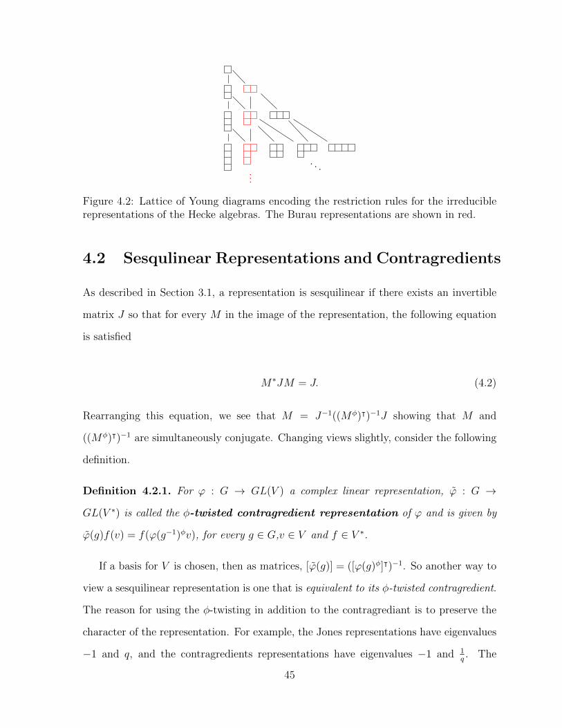
Remark 4.1.5. The lattice of Young diagrams has a chain of diagrams with two columns

and only one block in the second column, ...

. The representations corresponding to these

diagrams are the Burau representations. There is a natural symmetry of the lattice of

Young diagrams, so depending on the choice of convention, one could define the Burau

representations as the diagrams with exactly two rows, and one box in the second row.

The Burau representations are shown in red in Figure 4.2.

44

...

. . .

Figure 4.2: Lattice of Young diagrams encoding the restriction rules for the irreduciblerepresentations of the Hecke algebras. The Burau representations are shown in red.

4.2 Sesqulinear Representations and Contragredients

As described in Section 3.1, a representation is sesquilinear if there exists an invertible

matrix J so that for every M in the image of the representation, the following equation

is satisfied

M∗JM = J. (4.2)

Rearranging this equation, we see that M = J−1((Mφ)ᵀ)−1J showing that M and

((Mφ)ᵀ)−1 are simultaneously conjugate. Changing views slightly, consider the following

definition.

Definition 4.2.1. For ϕ : G → GL(V ) a complex linear representation, ϕ : G →

GL(V ∗) is called the φ-twisted contragredient representation of ϕ and is given by

ϕ(g)f(v) = f(ϕ(g−1)φv), for every g ∈ G,v ∈ V and f ∈ V ∗.

If a basis for V is chosen, then as matrices, [ϕ(g)] = ([ϕ(g)φ]ᵀ)−1. So another way to

view a sesquilinear representation is one that is equivalent to its φ-twisted contragredient.

The reason for using the φ-twisting in addition to the contragrediant is to preserve the

character of the representation. For example, the Jones representations have eigenvalues

−1 and q, and the contragredients representations have eigenvalues −1 and 1q. The

45

involution φ is necessary to return the 1q

eigenvalue back to a q.

This viewpoint combined with the following proposition gives a crucial perspective

for the proof of Theorem 4.0.1.

Proposition 4.2.2. If an absolutely irreducible matrix representation has an invertible

matrix J satisfying equation 4.2, then J is unique up to scaling.

Proof. Suppose there were two such matrices J1 and J2. Then equation 4.2 gives for all

matrices M in the representation,

J1MJ−11 = ((Mφ)ᵀ)−1 =J2MJ−12

⇒ (J−11 J2)−1M(J−11 J2) =M.

This shows that J−11 J2 is in the centralizer of the entire irreducible representation.

Schur’s Lemma gives that J−11 J2 = α·Id for some scalar α, and finally J2 = αJ1.

4.2.1 Proof of Theorem 4.0.1

Lemma 4.2.3. Every finite dimensional irreducible representation of the Hecke algebra

is equivalent to its φ-twisted contragediant representation, when q is a generic complex

number.

Proof. We can establish this result for n = 3. There are three non-equivalent irreducible

representations of H3(q) corresponding to the following Young diagrams.

Up to equivalence, the first two representations are one dimensional given by gi 7→ q

and gi 7→ −1, which are in fact equal to their φ-twisted contragredient representations.

The third representation is known to be the Burau representation for B3. As described

in Chapter 2, Squier showed that the Burau representations are sesquilinear and are

therefore equivalent to their φ-twisted contragediant.

46

Inductively moving forward, let ρ : Hn(q) → GL(V ) be a finite dimensional irre-

ducible representation and ρ be the φ-twisted contragredient representation of ρ. Up to

equivalence, ρ corresponds to a Young diagram λ. To show that ρ and ρ are equivalent,

it suffices to show that both representations correspond to the same λ. A Young diagram

is completely characterized by its list of (n − 1)-subdiagrams, which correspond to the

restriction of the representation to Hn−1(q). So it is enough to show that the restrictions

of ρ and ρ correspond to the same list of (n− 1)-subdiagrams.

Denoting ρ| = ρ|Hn−1(q), by Theorem 4.1.3 there is an equivalence T so that

Tρ|(h)T−1 =k⊕i=1

ρλi(h) for every h ∈ Hn−1(q),

where each λi is an (n−1)-subdiagram of λ, k is the number of (n−1)-subdiagrams of λ,

and ρλi is an irreducible representation of Hn−1(q) corresponding to λi. Choosing a basis

for V , the matrix for [Tρ|(h)T−1] is block diagonal. Taking the φ-twisted contragredient

of a block diagonal matrix preserves the block decomposition, which gives

([T φ]ᵀ)−1[ρ|(h)][T φ]ᵀ =k⊕i=1

[ρλi(h)] for every h ∈ Hn−1(q).

This equation shows that ρ| is equivalent to⊕

ρλi . Since each ρλi is an irreducible

representation of Hn−1(q), we can inductively assume that ρλi is equivalent to ρλi , for

all i ≤ k. Therefore, ρλi and ρλi correspond to the same Young diagram λi. Thus the

restrictions of ρ and ρ correspond to the same list of (n− 1)-subdiagrams.

Remark 4.2.4. While it would be elegant to have a proof of this result using character

theory, the generality of this approach allows a broader application to algebras that are

not deformations of the symmetric group.

Theorem 4.0.1. If ρ is an irreducible Jones representation of Bn and q generic unit

complex number close to 1, then there exists a non-degenerate, positive definite, sesquilin-

ear matrix J so that for all M in the image of ρ, (Mφ)ᵀJM = J .

47

Proof. Let ρ be a finite dimensional irreducible representation of Hn(q) over V . By

Lemma 4.2.3, ρ is equivalent to its φ-twisted contragredient representation ρ by an equiv-

alence T . Choose a basis for V and its dual basis for V ∗, let T be the matrix for T with

respect to these bases. We will use this matrix T to find the desired matrix J . Let

superscript ∗ denote the φ-twisted transpose of a matrix to ease computation. For all

g ∈ Hn(q), we get the following matrix equations.

T [ρ(g)]T −1 = [ρ(g)] = ([ρ(g)]−1)∗

⇒ (T −1)∗[ρ(g)]∗T ∗ = [ρ(g)]−1 (‡)⇒ T ∗[ρ(g)](T ∗)−1 = ([ρ(g)]−1)∗

This shows that T and T ∗ are two possible forms for ρ. By Proposition 4.2.2, T = αT ∗

for some α ∈ C. Applying ∗ again gives T = αα∗T and αα∗ = 1.

Define J = βT + β∗T ∗ = (αβ + β∗)T ∗ where β is as follows. (The need for β is to

ensure that J is invertible.) If α 6= −1, let β = 1 with gives that det J = det((α + 1)T )

which is nonzero. If α = −1, let β ∈ C so that β∗ 6= β. Then det J = det[(αβ+β∗)T ∗] =

det[(−β + β∗)T ] is nonzero. So in both cases, J is invertible.

Secondly, J is sesqulinear, that is J∗ = (βT + β∗T ∗)∗ = β∗T ∗ + βT = J . If M is a

matrix in the image of ρ, rearranging equation (‡) gives M∗T ∗M = T . So, inserting J

gives

M∗JM = M∗(αβ + β∗)T ∗M = (αβ + β∗)M∗T ∗M = (αβ + β∗)T = J.

It remains to show that J is positive definite. Taking q = 1, ρ is an irreducible

representation of the symmetric group Σn. As a linear representation of a finite group,

V admits an inner product that is invariant under the action of Σn, given by a positive

definite nondegenerate matrix J . Proposition 4.2.2 guarantees that J is unique up to

scaling. Since J |q=1 is also a form for this representation, it must be that J is a multiple

of J |q=1, which gives that J is positive definite for q = 1. Since J is Hermitian for unit

48

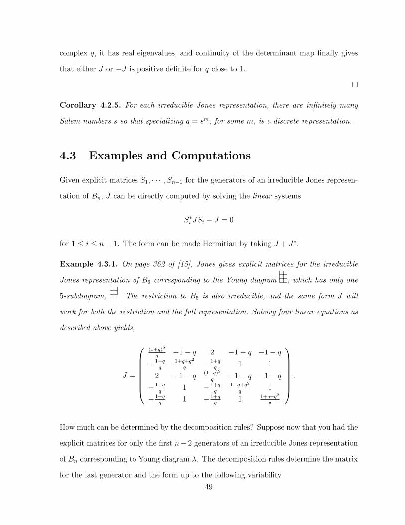
complex q, it has real eigenvalues, and continuity of the determinant map finally gives

that either J or −J is positive definite for q close to 1.

Corollary 4.2.5. For each irreducible Jones representation, there are infinitely many

Salem numbers s so that specializing q = sm, for some m, is a discrete representation.

4.3 Examples and Computations

Given explicit matrices S1, · · · , Sn−1 for the generators of an irreducible Jones represen-

tation of Bn, J can be directly computed by solving the linear systems

S∗i JSi − J = 0

for 1 ≤ i ≤ n− 1. The form can be made Hermitian by taking J + J∗.

Example 4.3.1. On page 362 of [15], Jones gives explicit matrices for the irreducible

Jones representation of B6 corresponding to the Young diagram , which has only one

5-subdiagram, . The restriction to B5 is also irreducible, and the same form J will

work for both the restriction and the full representation. Solving four linear equations as

described above yields,

J =

(1+q)2

q−1− q 2 −1− q −1− q

−1+qq

1+q+q2

q−1+q

q1 1

2 −1− q (1+q)2

q−1− q −1− q

−1+qq

1 −1+qq

1+q+q2

q1

−1+qq

1 −1+qq

1 1+q+q2

q

.

How much can be determined by the decomposition rules? Suppose now that you had the

explicit matrices for only the first n− 2 generators of an irreducible Jones representation

of Bn corresponding to Young diagram λ. The decomposition rules determine the matrix

for the last generator and the form up to the following variability.

49

• The matrix for the last generator is unique up to conjugation by any γ in the

centralizer of S1, · · · , Sn−2. So if Sn−1 is one choice of matrix for the last gen-

erator, any other choice of matrix for the last generator is of the form γ−1Sn−1γ.

Furthermore, after changing basis so the matrices for the first n − 2 generators

are block diagonal, then by Schur’s lemma every γ is block diagonal with scaled

identity matrices as the blocks.

• If J is a form for the representation 〈S1, · · · , Sn−2, Sn−1〉, then γ∗Jγ is a form for

the representation 〈S1, · · · , Sn−2, γ−1Sn−2γ〉.

Example 4.3.2. Consider the Young diagram , which has two 3-subdiagrams, , and

. These subdiagrams correspond to the reduced Burau representation of B3 and the

trivial representation. Forming an induced representation on B4 the first two generators

can be given by

S1 =

q 1 0

0 1 0

0 0 1

and S2 =

1 0 0

q −q 0

0 0 1

.The matrices R1 and R2 are two different possibilities for the third generator. These

matrices are conjugate by an element in the centralizer of 〈S1, S2〉 and ultimately give

rise to different but equivalent representations of B4.

R1 =

1 − q

q2+q+11

0 (−q−1)qq2+q+1

+ 1 q + 1

0q(q3+q2+q+1)

(q2+q+1)2− q3

q2+q+1

R2 =

1 − q

q2+q+13

0 (−q−1)qq2+q+1

+ 1 3(q + 1)

0q(q3+q2+q+1)3(q2+q+1)2

− q3

q2+q+1

The matrix J1 is the form for the representation 〈S1, S2, R1〉 and the matrix J2 is the

form for the representation 〈S1, S2, R2〉.

50

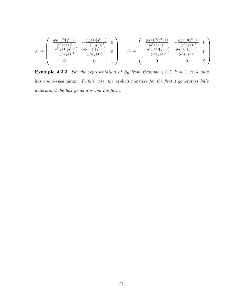
J1 =

q(q+1)2(q2+1)

(q2+q+1)3− q(q+1)(q2+1)

(q2+q+1)30

− q2(q+1)(q2+1)(q2+q+1)3

q(q+1)2(q2+1)(q2+q+1)3

0

0 0 1

J2 =

q(q+1)2(q2+1)

(q2+q+1)3− q(q+1)(q2+1)

(q2+q+1)30

− q2(q+1)(q2+1)(q2+q+1)3

q(q+1)2(q2+1)(q2+q+1)3

0

0 0 9

Example 4.3.3. For the representation of B6 from Example 4.3.1, k = 1 as λ only

has one 5-subdiagram. In this case, the explicit matrices for the first 4 generators fully

determined the last generator and the form.

51

Chapter 5

BMW Representations

5.1 The BMW Algebras

The BMW algebras were discovered in the 1980’s by Joan Birman and Hans Wenzl

in [4], and simultaneously by Jun Murakami [25]. Following the notation of [4] and Zinno

in [34], the BMW algebras Cn(l,m) are a two parameter, l and m, family of algebras

with n− 1 generators. The invertible generators are denoted G1, · · · , Gn−1 which satisfy

the following relations in terms of non-invertible elements denoted by Ei as follows:

GiGj = GjGi for |i− j| > 1 (5.1)

GiGi+1Gi = Gi+1GiGi+1 (5.2)

G2i = m(Gi + l−1Ei)− 1. (5.3)

There are additional relations:

52

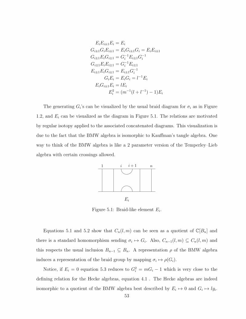
EiEi±1Ei = Ei

Gi±1GiEi±1 = EiGi±1Gi = EiEi±1

Gi±1EiGi±1 = G−1i Ei±1G−1i

Gi±1EiEi±1 = G−1i Ei±1

Ei±1EiGi±1 = Ei±1G−1i

GiEi = EiGi = l−1Ei

EiGi±1Ei = lEi

E2i = (m−1(l + l−1)− 1)Ei

The generating Gi’s can be visualized by the usual braid diagram for σi as in Figure

1.2, and Ei can be visualized as the diagram in Figure 5.1. The relations are motivated

by regular isotopy applied to the associated concatenated diagrams. This visualization is

due to the fact that the BMW algebra is isomorphic to Kauffman’s tangle algebra. One

way to think of the BMW algebra is like a 2 parameter version of the Temperley–Lieb

algebra with certain crossings allowed.

i i+ 11 n

Ei

Figure 5.1: Braid-like element Ei.

Equations 5.1 and 5.2 show that Cn(l,m) can be seen as a quotient of C[Bn] and

there is a standard homomorphism sending σi 7→ Gi. Also, Cn−1(l,m) ⊆ Cn(l,m) and

this respects the usual inclusion Bn−1 ⊆ Bn. A representation ρ of the BMW algebra

induces a representation of the braid group by mapping σi 7→ ρ(Gi).

Notice, if Ei = 0 equation 5.3 reduces to G2i = mGi − 1 which is very close to the

defining relation for the Hecke algebras, equation 4.1 . The Hecke algebras are indeed

isomorphic to a quotient of the BMW algebra best described by Ei 7→ 0 and Gi 7→ lgi.

53

However, the Hecke algebra’s are not equal to a subalgebra of the BMW because of an

incompatibility of their multiplicative structures, see [34] for more detail. This isomorphic

copy of the Hecke algebra inside Cn(l,m) is typically denoted by Hn.

The dimension of Cn(l,m) is (2n)!2nn!

which has been proved in many ways, but directly

computed in [24] and [4]. BMW algebras are a deformation of the Brauer algebras

in the same way that the Hecke algebras are a deformation of the complex algebra of

the symmetric group. The Brauer algebras can be obtained from Cn(l,m) by simple

re-parameterization and specialization of l = −i, see Section 5 of [4].

5.2 The BMW Representations

Recall from Section 4.1 that the irreducible representations of the Hecke algebras are

parameterized by the Young diagrams with the standard Young lattice describing the

restriction rules in Figure 4.2. Analogously, the irreducible representations of the BMW

algebras Cn(l,m) are parameterized by a Bratteli diagram whose vertices are Young Di-

agram as show in Figure 5.2, but the restriction rule is quite different from the standard

Young lattice. The new restriction rule is:

BMW restriction rule: A Young diagram λn in row n is connected to a Young dia-

gram λn+1 in row n+ 1 if λn+1 is obtained from λn by adding or removing a single box.

As depicted in Figure 5.2, the standard Young lattice occurs in the Bratteli diagram

and corresponds to Hn the subalgebra of Cn(l,m) isomorphic to the Hecke algebras. The

induced representations of the braid group coming from the subalgebra Hn are the Jones

representations, [34].

Notice that any λn+1 in the n + 1’st row is completely determined by the the set of

diagrams in the n’th row connecting to λn+1. We can describe this property by saying

54

∅

∅

......

. . .

Figure 5.2: Bratteli diagrams for the restriction rules of the irreducible representationsof the BMW algebras. The Lawrence-Krammer representation is shown in red.

a diagram is determined up to equivalence by the restriction rule (equivalent as in the

sense of Definition 4.1.4 from Section 4.1).

Similar to how the the Burau representation is one irreducible summand of the Jones

representations, the Lawrence-Krammer representation is one summand of the BMW

representations, colored red in Figure 5.2. The Lawrence-Krammer representation was

first discovered by Ruth Lawrence [19] and famously studied by Daan Krammer and

Stephen Bigelow. It was originally defined as a homological representations coming from

a mapping class group action, but was proved later by Zinno [34] to come from the BMW

algebras.

5.3 Explicit Matrices for the BMW Representations

To compute the three 1-dimensional BMW representations of B2, first we choose a ba-

sis for the algebra as a vector space over C(l,m), for example 1, G,G−1. Then we

let the G act on this ordered basis to get a 3 × 3 representation of B2. This left reg-

ular representation is a direct sum of thee 1-dimensional representations, shown in the

diagonalization.

55

0 −ml− 1 1

1 m+ 1l

00 1

l0

∼ 1

l0 0

0 12(m− 1

√−4 +m2) 0

0 0 12(m+

√−4 +m2)

So the three 1-dimensional representations are ϕ1(G) = 1

l, ρ1(G) = 1

2(m−1

√−4 +m2)

and ρ2(G) = 12(m+ 1

√−4 +m2).

ρi(E) =1

m(ρi(G)− ρi(G)−1)− 1 = 0

Which shows that both ρi’s are actually representations of the Hecke algebra so they

correspond to the two Young diagrams in row 2 of the Bratteli diagrams. The third

representation ϕ corresponds to the ∅ diagram.

Example 5.3.1. In [4], Birman and Wenzl computed the representation of B3 corre-

sponding to the single box Young diagram.

σi 7→

l−1 m 00 m 10 −1 0

, σ2 7→

0 0 −10 l−1 l−1m1 0 m

5.4 Sesquilinearity

Using Morse theoretic arguments, Budney proved that the Lawrence Krammer is sesquilin-

ear [7]. In this section, we will extend Budney’s result to all of the BMW representations.

Theorem 5.4.1. If ρ is an irreducible BMW representation of Bn then there exists a

non-degenerate, sesquilinear matrix J so that for all M in the image of ρ, M∗JM = J .

To make sense of the ∗ operation in Theorem 5.4.1, we need to define an involution

of the coefficients. The relevant involution for the BMW algebra is l 7→ 1l, m 7→ m,

and α 7→ 1α

where m = α + 1α

. We will denote this involution by φ. So to show

sesquilineararity in this context is to show that the representations are equivalent to

their φ-twisted contragrediant representation using φ to define ∗.56

The proof of Theorem 5.4.1 is exactly analogous to the proof of Theorem 4.0.1 showing

that the Jones representations are sesquilinear, excluding the positive definite argument.

It is only necessary to prove the following Lemma.

Lemma 5.4.2. If ρ is an irreducible BMW representation of Bn, then ρ is equivalent to

its φ-twisted contragredient representation.

Proof. Analogously to Lemma 4.2.3, we will prove this result by induction on n.

Let ρ be an irreducible BMW representation of B2. As shown in the Section 5.3,

there are three possible 1-dimensional representations given by ϕ1(G) = 1l, ρ1(G) =

12(m− 1

√−4 +m2) and ρ2(G) = 1

2(m+ 1

√−4 +m2).

In the diagonalization process to compute these representations, we introduced a

square-root term√−4 +m2. Extending φ to the field including this term, we define

φ(√−4 +m2) = −

√−4 +m2. Each of these one-dimensional representations are equal

to thier φ-twisted contragredient representation.

Inductively moving forward, let ρ be an irreducible BMW representation of Bn, and

ρ be the φ-twisted contragadient of ρ. Let ρ correspond to Young diagram λ1 and ρ

correspond to λ2. As described in Section 5.2, λ1 and λ2 are completely determined by

the BMW restriction rule. The inductive step is the exactly the same as in Lemma 4.2.3.

5.4.1 Positive-Definiteness

One motivation for showing the BMW representations are sesquilinear is to find dis-

crete specializations of the parameters. Theorem 3.3.3 proved that we can find infinitely

many discrete specializations of a parameterized representation, given certain require-

ments about the positive definiteness of the sesquilinear form J . This section discusses

the positive definiteness of the forms for the BMW representations.

57

Conjecture: The forms for the BMW representations, found in Theorem 5.4.1, are pos-

itive definite for specializations in some open neighborhood in C2.

This conjecture has been experimentally verified for several of the smaller indexed

BMW representations as described in Examples 5.4.3 and 5.4.4 to follow, but has not

been proven in general. Since the proof of Theorem 5.4.1 was completely analogous to

that of Theorem 4.0.1, at first glance there is hope to repeat the positive definiteness

argument that worked for the Jones representations. However, there is a major obstacle

that prevents this approach from generalizing to the BMW representations. The forms

for the Jones representations found in Theorem 4.0.1 were proven to be positive definite in

a complex neighborhood of 1 by using the fact that the Hecke algebras are a deformation

of the complex symmetric algebras. That is at q = 1, Hq(n) collapses to C[Σn]. Since

Σn is a finite group, its representations are unitary. Now in a similar way, the BMW

algebras are a deformation of the Brauer algebras. However it is unknown whether the

irreducible representations of the Brauer algebras are unitary/sesquilinear or not. So

some further investigation into the representation theory of the Brauer algebras could

lead to a general proof the conjecture.

Example 5.4.3.

One of the BMW representation of B4 is given by:

σ1 7→

1a

0 0 0 0 0

0 0 0 0 −1 0

0 0 0 0 0 −1

0 0 0 1L

a+ 1a

L

a(a+ 1a)

L

0 1 0 0 a+ 1a

0

0 0 1 0 0 a+ 1a

σ2 7→

0 0 −1 0 0 0

0 1L

a+ 1a

La+ 1

a0 0

1 0 a+ 1a

0 0 0

0 0 0 a+ 1a

1 0

0 0 0 −1 0 0

0 0 0 0 0 1a

58

σ3 7→

1L

a+ 1a

0 0a+ 1

a

a0

0 a+ 1a

1 0 0 0

0 −1 0 0 0 0

0 0 0 1a

0 0

0 0 0 0 a+ 1a

1

0 0 0 0 −1 0

J can be computed as the diagonal matrix with the following entries on the diagonal

J1,1 =2

J2,2 =− 2a (L2 + 1) (2a2L− aL2 − a+ 2L)

(a− L)2(aL− 1)2

J3,3 =2 (L2 + 1) (a3 + L) (a3L+ 1)

a(a− L)(aL− 1) (2a2L− aL2 − a+ 2L)

J4,4 =2(a+ L) (a5L2 + a4L− a3L2 − a3 + a2L3 + a2L− aL2 − L)

a (L2 + 1) (a3 + L) (aL− 1)

J5,5 =2(a+ L)(aL+ 1) (a3L+ 1) (2a3L2 + a3 + a2L+ aL2 + L3 + 2L)

a (L2 + 1) (aL− 1) (a5L2 + a4L− a3L2 − a3 + a2L3 + a2L− aL2 − L)

J6,6 =− 2 (a5 − L) (a+ L)(aL+ 1) (a3L+ 1)

a3(aL− 1) (2a3L2 + a3 + a2L+ aL2 + L3 + 2L)

A short computation shows that J(a, l) = J(i, 1) = 2Id, giving a point where J is

positive definite. Continuity of the determinant implies that J is positive definite in a

neighborhood of (i, 1) on the complex torus. It is difficult to determine explicitly the

radius of this neighborhood. However, one can choose a Salem number and through trial

and error, find powers of the Salem number that are very close to (i, 1) where the form

stays positive definite. Taking the Salem number S = 12

+ 1√2

+ 1

2√−1+2

√2, specializing

a = S15 and L = S3 leaves J positive definite at the complex places of OQ(S). So this

representation is discrete at the specialization a = S15, L = S3.

59

Example 5.4.4.

Taking m = 0 in the BMW algebra yields a quotient of the C[Bn] where each genera-

tor G2i = −1, or rather each generator has order 4. It is known that this quotient of the

braid group yields a finite group exactly when n = 3 [18, pg 81]. So with this information,

we know there is a neighborhood of m = 0 where all of the BMW representations of B3

have a positive definite form.

60

Chapter 6

Lattices and Commensurability

6.1 Commensurability

The irreducible Jones representations corresponding to rectangular Young diagrams, as

in Example 4.3.1, are particularly interesting and lead to some further questioning. What

is special about these representations is that they each have only one (n−1)-subdiagram.

This implies that both the restriction representation and the full representation are ir-

reducible, of the same dimension and use the same form J . Both representations map

into the same unitary group. How can we mimic this situation for the other irreducible

Jones representations for the non-rectangular diagrams? Can we get two representations

to map into the “same” unitary group? The answer is yes! The approach is to fix a

representation and specialize to two different powers of the same Salem number. The

ring of integers OK will stay the same, but the defining sesquilinear forms might be very

different.

Recall the notation of K, L, OK and φ from Section 3.3. In general, fixing a number

ring OK and dimension m, the group Um(J, φ,OK) is determined by the form J . Notice

that Um(J, φ,OK) = Um(λJ, φ,OK) for every λ ∈ L, and that the form J is not completely

unique. This motivates that following definition.

61

Definition 6.1.1. Matrices J and H are equivalent over K if Q∗JQ = λH for some

Q ∈ GLm(K) and λ ∈ Fix(φ).

It would be nice if equivalent forms gave rise to equal unitary groups, but this is

not true in general. However, in the careful scenario that the unitary group is a lat-

tice in SL(R), then changing the form by equivalence yields “the same” lattice, up to

commensurability in the following sense.

Definition 6.1.2. Two groups G1 and G2 are commensurable if there are finite index

subgroups H1 ⊆ G1 and H2 ⊆ G2 so that H1 is isomorphic to H2.

Definition 6.1.3. A lattice in a semisimple Lie group G is a discrete subgroup of G

with finite covolume.

For our purposes, we will take G = SLm(R) or PSLm(R).

Proposition 6.1.4. Assume SUm(J1, φ,OK) and SUm(J2, φ,OK) are lattices in SLm(R).

If J1 and J2 are equivalent over K, then SUm(J1, φ,OK) is commensurable to SUm(J2, φ,OK)

Proof. Let λJ1 = Q∗J2Q for some Q ∈ GLm(K) and λ ∈ Fix(φ). For notational clarity,

denote SU(Ji,OK) = SUm(Ji, φ,OK).

Since scalar multiplication commutes with matrix multiplication, then M∗JM = J

if and only if M∗λJM = λJ . So scaling the form preserves the unitary group, and

with out loss of generality we may assume λ = 1. It is easy to see that M∗JM = J

if and only if (Q∗M∗Q∗−1)(Q∗JQ)(Q−1MQ) = Q∗JQ, which seems like it implies that

SU(Q∗J1Q,OK) = Q−1SU(J1,OK)Q. However, since Q has coefficients in K, Q−1MQ

may not have coefficients in OK , so we can only conclude that Q−1SU(J,OK)Q ⊆

SU(Q∗JQ,K). To avoid this, we need to pass to a finite index subgroup.

Since K is the ring of fractions of OK , then there exists γ ∈ OK so that γQ ∈

Mm(OK). As a ring of integers of an algebraic extension, OK is a Dedekind domain and

every quotient is finite. So OK/〈γ2〉 is finite and SU(J1,OK/〈γ2〉) is finite. The kernel

N of the quotient map SU(J1,OK)→ SU(J1,OK/〈γ2〉) has finite index in SU(J1,OK).

62

Any element B in the kernel has the form B = Id+γ2A for some matrix A ∈Mm(OK).

Inserting Q∗J2Q for J1 into the equation B∗J1B = J1, gives that that QBQ−1 fixes the

form J2. Because Q has coefficients over K, QBQ−1 has coefficients in K and not

necessarily in OK . However, since QBQ−1 = Id + (γQ)A(γQ−1), and both A and γQ

are integral, then QBQ−1 is also integral. Thus QBQ−1 ∈ SU(J2,OK).

Since SU(J1,OK) is a lattice, and N is a finite index subgroup, then N is also a

lattice in SL(R) with finite covolume. Thus QNQ−1 has finite covolume in SL(R) and

is therefore a lattice in G. So QNQ−1 is a sublattice of SU(J2,OK) and must have finite

index.

This shows that N is a finite index subgroup SU(J1,OK) and QNQ−1 is finite index

in SU(J2,OK).

So how does this lattice information apply to the Jones representations? Firstly, after

a rescaling and reparameterization, the Jones representations can be made to have deter-

minant ±1, allowing the image to land in an PSU(J, φ,OK) instead of just U(J, φ,OK).

Secondly, an arithmetic group theory result of Harish-Chandra, that is formalized in our

setting in Chapter 6 of Witte [23], states that SUm(J, φ,OK) is a lattice in SLm(R) under

the exact Salem number circumstances as required by Theorem 3.3.3. So we can restate

Corollary 4.2.5 using this new vocabulary.

Corollary 6.1.5. For each irreducible Jones representation, after a change of parameter,

there are infinitely many Salem numbers s so that specializing q to a powers of s maps

the braid group into a lattice in PSLm(R).

Proof. Let ρq be an irreducible Jones representation of dimension m. The images of the

braid generators under ρq have determinant ±qk for some k ∈ N. After a change of

variable q = ym and scaling the generators by 1ym−k

, this adjusted representation ρy maps

into PSUm(Jy,Z[y±1]).

The subgroup B2n of squared braids is a non-central normal subgroup of Bn of finite

63

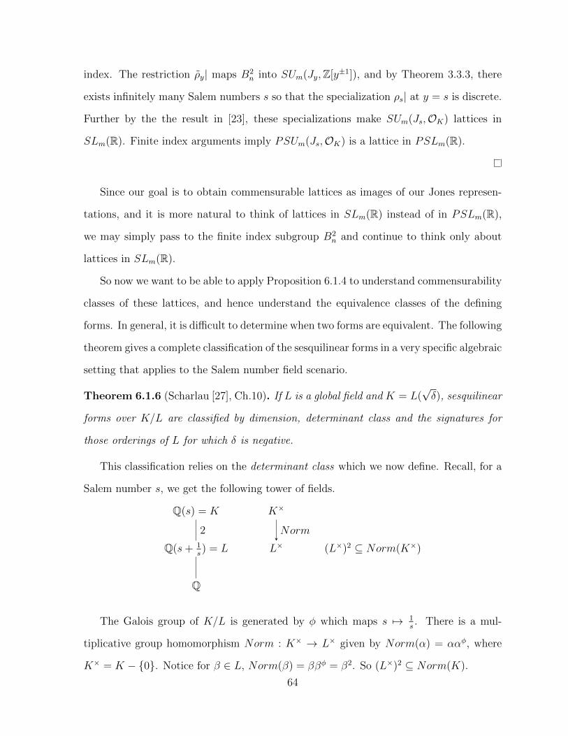
index. The restriction ρy| maps B2n into SUm(Jy,Z[y±1]), and by Theorem 3.3.3, there

exists infinitely many Salem numbers s so that the specialization ρs| at y = s is discrete.

Further by the the result in [23], these specializations make SUm(Js,OK) lattices in

SLm(R). Finite index arguments imply PSUm(Js,OK) is a lattice in PSLm(R).

Since our goal is to obtain commensurable lattices as images of our Jones represen-

tations, and it is more natural to think of lattices in SLm(R) instead of in PSLm(R),

we may simply pass to the finite index subgroup B2n and continue to think only about

lattices in SLm(R).

So now we want to be able to apply Proposition 6.1.4 to understand commensurability

classes of these lattices, and hence understand the equivalence classes of the defining

forms. In general, it is difficult to determine when two forms are equivalent. The following

theorem gives a complete classification of the sesquilinear forms in a very specific algebraic

setting that applies to the Salem number field scenario.

Theorem 6.1.6 (Scharlau [27], Ch.10). If L is a global field and K = L(√δ), sesquilinear

forms over K/L are classified by dimension, determinant class and the signatures for

those orderings of L for which δ is negative.

This classification relies on the determinant class which we now define. Recall, for a

Salem number s, we get the following tower of fields.

Q(s) = K K×

Q(s+ 1s) = L L× (L×)2 ⊆ Norm(K×)

Q

2 Norm

The Galois group of K/L is generated by φ which maps s 7→ 1s. There is a mul-

tiplicative group homomorphism Norm : K× → L× given by Norm(α) = ααφ, where

K× = K − 0. Notice for β ∈ L, Norm(β) = ββφ = β2. So (L×)2 ⊆ Norm(K).

64

Definition 6.1.7. The determinant class of a sesquilinear form H over K/L is the

coset of det(H) in K×/Norm(K×),

[det(H)] = det(H)Norm(K).

Taking δ = (s − 1s)2, K can be rewritten as K = L(

√δ). Thus we can restate

Scharlau’s classification in the specific context of Salem numbers.

Theorem 6.1.8 (Scharlau restated). Sesquilinear forms over K/L are classified by di-

mension, determinant class and the signatures for those orderings of L for which (s− 1s)2

is negative.

In odd dimension, it is very simple to show that all sesquilinear forms have the same

determinant class, up to scaling. However, for even dimension, the situation is very

unclear.

Proposition 6.1.9. For every odd dimensional invertible sesquilinear matrices H and

J over K, [det(H)] = [det(λJ)] for λ ∈ L.

Proof. Let H and J be sesquilinear matrices over K of dimension 2k + 1. Hermitian

guarantees both H and J are diagonalizable with diagonal entrees fixed by φ. So, the

determinant of both H and J are elements in L. Let dH and dJ denote the nonzero

determinants of both H and J . Thus

dH =dHdJdJ

mod(L×)2

≡ (dHdJ

)2k+1dJ = det(dHdJJ).

Since (L×)2 ⊆ Norm(K), then H and λJ have the same determinant class for λ = dHdJ∈

L.

As a result, to determine whether two forms of the same odd dimension are equivalent,

it suffices only to do check they have the same signatures.

Theorem 6.1.10. For Jt a sesquilinear form that is positive definite for t in a neighbor-

hood η of 1, there are infinitely many Salem numbers s and integers n,m, so that in all

65

odd dimension, SU2k+1(Jsn , φ,OK) and SU2k+1(Jsm , φ,OK) are commensurable, discrete

groups.

Proof. By Lemma 3.3.2 there are infinitely many Salem numbers s and integers n,m so

that every complex Galois conjugate of sm and sn lie in η. Fix one such Salem number

s, and K,L, and δ as above.

By Theorem 6.1.6, sesquilinear forms are completely classified by dimension, deter-

minant class, and the signatures for the places of L for which (s − 1s)2 is negative. By

Proposition 6.1.9, Jsn and λJsm have the same determinant class for λ in L, namely

λ = det Jsndet Jsm

.

Let σ be a complex placement of L. Then σ(sm) is a complex Galois conjugate of sm,

and similarly for σ(sn) and sn. Since n and m were chosen so that all of the complex

Galois conjugate of sm and sn have arguments in η, then Jσ(sm) and Jσ(sn) are positive

definite. Moreover, det Jsndet Jsm

and σ( det Jsndet Jsm

) are both positive, making λ > 0. So regardless

of whether σ((s− 1s)2) is positive or negative, the forms Jσ(si) have the same signature.

Thus, Jsn is equivalent to λJsm , and SU(Jsn , φ,OK) is commensurable to SU(Jsm , φ,OK).

The groups are discrete by Theorem 3.2.3.

Corollary 6.1.11. Let ρt : G → SL2k+1(Z[t, t−t]) be a group representation with a

parameter t. Suppose there exists a matrix Jt so that:

1. for all M in the image of ρt, M∗JtM = Jt, where M∗(t) = Mᵀ(1

t),

2. Jt = (J 1t)ᵀ,

3. Jt is positive definite for t in an neighborhood η of 1

Then, there exists infinitely many Salem numbers s, so that for infinitely many integers

n,m the specializations ρsm at t = sm and ρsn at t = sn map into commensurable lattices

of SL2k+1(R).

66

lattice

lattice

lattice

Bn

SL2k+1(R)

Figure 6.1

Example 6.1.12. The reduced Burau representation of B4 is 3 dimensional and, after the

appropriate rescaling to have determinant 1, satisfies Corollary 6.1.11. So certain powers

of the specializations in Example 3.4.2 map into commensurable lattices in SL3(R).

67

Bibliography

[1] Emil Artin. Theorie der Zopfe. Abh. Math. Sem. Univ. Hamburg, 4(1):47–72, 1925.

[2] Stephen Bigelow. The Burau representation is not faithful for n = 5. Geom. Topol.,

3:397–404, 1999.

[3] Stephen Bigelow. Does the Jones polynomial detect the unknot? J. Knot Theory

Ramifications, 11(4):493–505, 2002. Knots 2000 Korea, Vol. 2 (Yongpyong).

[4] Joan S. Birman and Hans Wenzl. Braids, link polynomials and a new algebra. Trans.

Amer. Math. Soc., 313(1):249–273, 1989.

[5] N. Bourbaki. Springer Verlag, Berlin Heidelberg, 1972.

[6] Tara Brendle, Dan Margalit, and Andrew Putman. Generators for the hyperelliptic

Torelli group and the kernel of the Burau representation at t = −1. Invent. Math.,

200(1):263–310, 2015.

[7] Ryan D. Budney. On the image of the Lawrence-Krammer representation. J. Knot

Theory Ramifications, 14(6):773–789, 2005.

[8] Werner Burau. ”about Z petting groups and correspondence twisted V leases. dep.

Math. Sem. Univ. Hamburg, 11(1):179–186, 1935.

[9] R. H. Fox. A quick trip through knot theory. In Topology of 3-manifolds and related

topics (Proc. The Univ. of Georgia Institute, 1961), pages 120–167. Prentice-Hall,

Englewood Cliffs, N.J., 1962.

68

[10] Jennifer M. Franko. Braid group representations arising from the Yang-Baxter equa-

tion. J. Knot Theory Ramifications, 19(4):525–538, 2010.

[11] Michael H. Freedman, Michael J. Larsen, and Zhenghan Wang. The two-eigenvalue

problem and density of Jones representation of braid groups. Comm. Math. Phys.,

228(1):177–199, 2002.

[12] Louis Funar and Toshitake Kohno. On Burau’s representations at roots of unity.

Geom. Dedicata, 169:145–163, 2014.

[13] Tetsuya Ito. A kernel of a braid group representation yields a knot with trivial knot

polynomials. Math. Z., 280(1-2):347–353, 2015.

[14] Craig H. Jackson. Braid group representations. 2001.

[15] V. F. R. Jones. Hecke Algebra Representations of Braid Groups and Link Polyno-

mials. Annals of Mathematics, 126(2):335–388, 1987.

[16] Michael Kapovich. Hyperbolic Manifolds and Discrete Groups. 2010.

[17] A. Yu. Kitaev. Quantum computations: algorithms and error correction. Uspekhi

Mat. Nauk, 52(6(318)):53–112, 1997.

[18] Bohdan I. Kuripita Kunio Murasugi. A study of Braids. Kluwer Academic Press,

1999.

[19] R. J. Lawrence. Homological representations of the Hecke algebra. Comm. Math.

Phys., 135(1):141–191, 1990.

[20] D. D. Long and M. Paton. The Burau representation is not faithful for n ≥ 6.

Topology, 32(2):439–447, 1993.

[21] Darren Long. A note on the normal subgroups of mapping class groups. Math. Proc.

Camb. Phil. Soc, 99:295 – 303, 1986.

69

[22] John Atwell Moody. The Burau representation of the braid group Bn is unfaithful

for large n. Bull. Amer. Math. Soc. (N.S.), 25(2):379–384, 1991.

[23] Dave Witte Morris. Introduction to Arithmetic Groups. Deductive Press, 2015.

[24] H. R. Morton. A basis for the birman-wenzl algebra. arXiv:1012.3116v1 [math.QA],

2010.

[25] Jun Murakami. The Kauffman polynomial of links and representation theory. Osaka

J. Math., 24(4):745–758, 1987.

[26] John Ratcliffe. Foundations of Hyperbolic n-Manifolds. Springer, 2nd edition, 2006.

[27] Winfried Scharlau. Quadratic and Hermitian Forms. Springer-Verlag, 1985.

[28] Craig C. Squier. The Burau representation is unitary. Proc. Amer. Math. Soc.,

90(2):199–202, 1984.

[29] James van Buskirk. Braid groups of compact 2-manifolds with elements of finite

order. Trans. Amer. Math. Soc., 122:81–97, 1966.

[30] T. N. Venkataramana. Image of the burau representation at d-th roots of unity.

Annals of Mathematics, 179:1041–1083, 2014.

[31] Hans Wenzl. Hecke Algebras of Type an and Subfactors. Inventiones mathematicae,

92(2):349–384, 1988.

[32] Norbert J. Wielenberg. Discrete Moebius groups: fundamental polyhedra and con-

vergence. Amer. J. Math., 99(4):861–877, 1977.

[33] Yufei Zhao. Young Tableaux and the Representations of the Symmetric Group.

[34] Matthew G. Zinno. On Krammer’s representation of the braid group. Math. Ann.,

321(1):197–211, 2001.

70

Discrete Representations of the Braid Groups · 2019-06-13 · Nancy C. Scherich CV Research...

Documents

Transcript of Discrete Representations of the Braid Groups · 2019-06-13 · Nancy C. Scherich CV Research...