Discrete Fourier Transformation(DFT)

1

Eigen-Analysis(System or Linear Transformation)

2

Eigenvector and Eigenvalues

• Given matrix 𝐴

• Eigenvectors 𝑣 are input signals that emerge at the system output unchanged (except for a scaling by the eigenvalue 𝜆𝑘) and so are somehow “fundamental” to the system

• Using this, we can find the following equation

• We can change to

3

Eigen-analysis of LTI Systems (Finite-Length Signals)

• For length-𝑁 signals, 𝐻 is an 𝑁 × 𝑁 circulent matrix with entries

where ℎ is the impulse response

• Goal: calculate the eigenvectors and eigenvalues of 𝐻

– Fact: the eigenvectors of a circulent matrix (LTI system) are the complex harmonic sinusoids

– The eigenvalue 𝜆𝑘 ∈ ℂ corresponding to the sinusoid eigenvectors 𝑠𝑘 is called the frequency response at frequency 𝑘 since it measures how the system “responds” to 𝑠𝑘

4

Eigenvector of LTI Systems (Finite-Length Signals)

• Prove that

– harmonic sinusoids are the eigenvectors of LTI systems simply by computing the circular convolution with input 𝑠𝑘 and applying the periodicity of the harmonic sinusoids

• 𝜆𝑘 means the number of 𝑠𝑘 in ℎ[𝑛] ⇒ similarity

5

Eigenvector Matrix of Harmonic Sinusoids

• Stack 𝑁 normalized harmonic sinusoid 𝑠𝑘 𝑘=0𝑁−1 as columns into an 𝑁 × 𝑁 complex orthonormal basis

matrix

6

Signal Decomposition by Harmonic Sinusoids

7

Basis

• A basis {𝑏𝑘} for a vector space 𝑉 is a collection of vectors from 𝑉 that linearly independent and span 𝑉

• Basis matrix: stack the basis vectors 𝑏𝑘 as columns

• Using this matrix 𝐵, we can now write a linear combination of basis elements as the matrix/vector product

8

Orthonormal Basis

• An orthogonal basis 𝑏𝑘 𝑘=0𝑁−1 for a vector space 𝑉

– a basis whose elements are mutually orthogonal

• An orthonormal basis 𝑏𝑘 𝑘=0𝑁−1 for a vector space 𝑉

– a basis whose elements are mutually orthogonal and normalized in the 2-norm

9

Orthonormal Basis

• 𝐵 is a unitary matrix

10

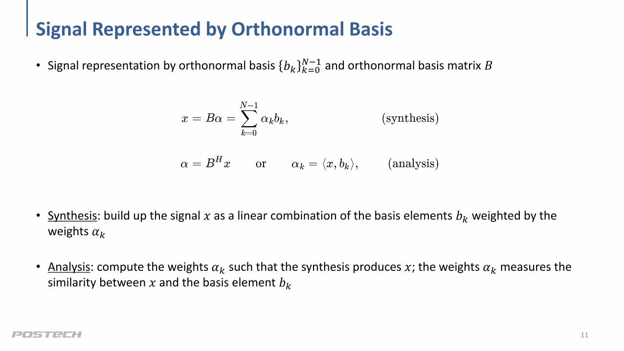
Signal Represented by Orthonormal Basis

• Signal representation by orthonormal basis 𝑏𝑘 𝑘=0𝑁−1 and orthonormal basis matrix 𝐵

• Synthesis: build up the signal 𝑥 as a linear combination of the basis elements 𝑏𝑘 weighted by the weights 𝛼𝑘

• Analysis: compute the weights 𝛼𝑘 such that the synthesis produces 𝑥; the weights 𝛼𝑘 measures the similarity between 𝑥 and the basis element 𝑏𝑘

11

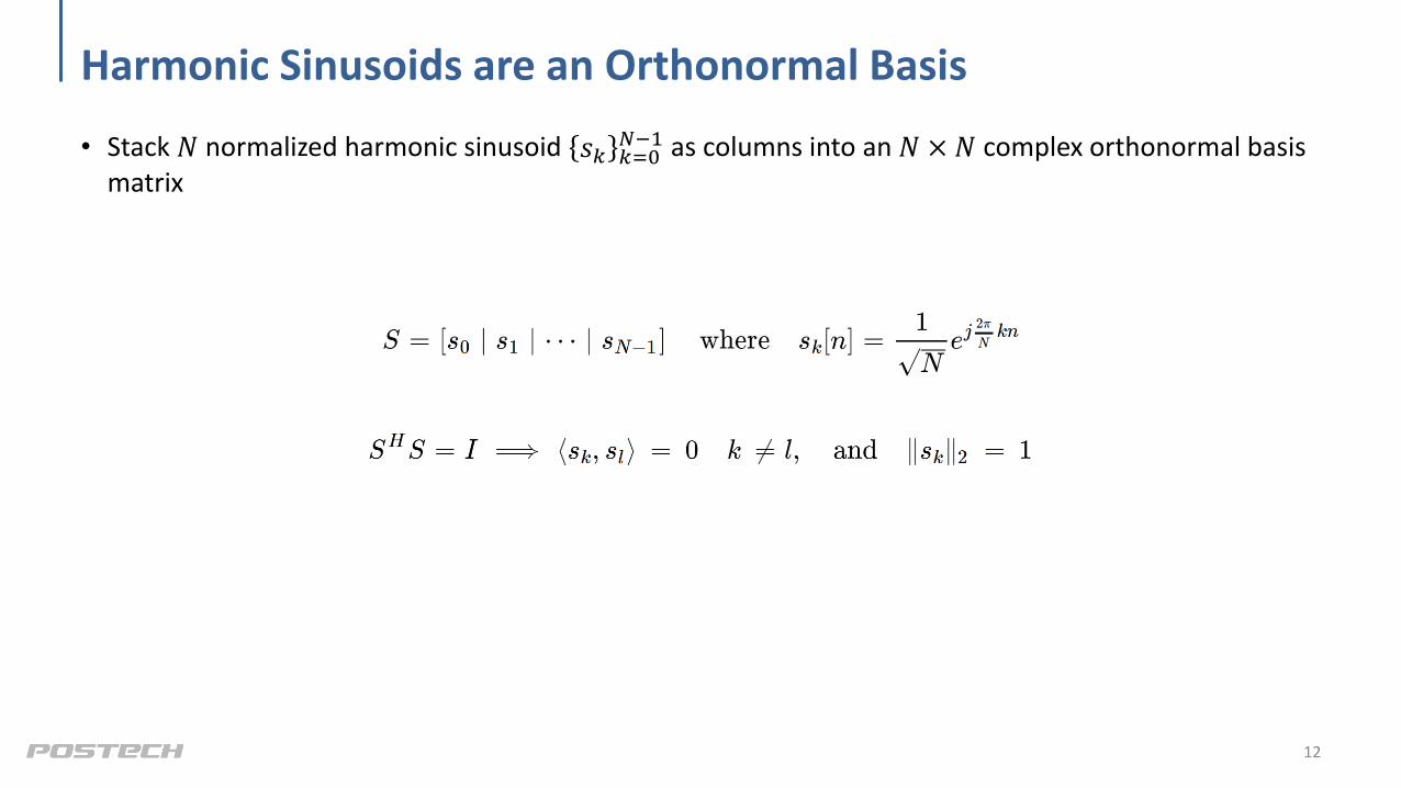
Harmonic Sinusoids are an Orthonormal Basis

• Stack 𝑁 normalized harmonic sinusoid 𝑠𝑘 𝑘=0𝑁−1 as columns into an 𝑁 × 𝑁 complex orthonormal basis

matrix

12

Discrete Fourier Transform (DFT)

13

DFT and Inverse DFT

• Jean Baptiste Joseph Fourier had the radical idea of proposing that all signals could be represented as a linear combination of sinusoids

• Analysis (Forward DFT)

– The weight 𝑋[𝑘] measures the similarity between 𝑥 and the harmonic sinusoid 𝑠𝑘– It finds the “frequency contents” of 𝑥 at frequency 𝑘

14

DFT and Inverse DFT

• Jean Baptiste Joseph Fourier had the radical idea of proposing that all signals could be represented as a linear combination of sinusoids

• Synthesis (Inverse DFT)

– It is returning to time domain

– It builds up the signal 𝑥 as a linear combination of 𝑠𝑘 weighted by the 𝑋[𝑘]

15

Unnormalized DFT

• Normalized forward and inverse DFT

• Unnormalized forward and inverse DFT

16

Harmonic Sinusoids are an Orthonormal Basis

• Stack 𝑁 normalized harmonic sinusoid 𝑠𝑘 𝑘=0𝑁−1 as columns into an 𝑁 × 𝑁 complex orthonormal basis

matrix

17

Eigen-decomposition and Diagonalization

• 𝐻 is circulent LTI System matrix

• 𝑆 is harmonic sinusoid eigenvectors matrix (corresponds to DFT/IDFT)

• Λ is eigenvalue diagonal matrix (frequency response)

• The eigenvalues are the frequency response (unnormalized DFT of the impulse response)

• Place the 𝑁 eigenvalues 𝜆𝑘 𝑘=0𝑁−1 on the diagonal of an 𝑁 × 𝑁 matrix

18

Eigen-decomposition and Diagonalization

• 𝐻 is circulent LTI System matrix

• 𝑆 is harmonic sinusoid eigenvectors matrix (corresponds to DFT/IDFT)

• Λ is eigenvalue diagonal matrix (frequency response)

19

Eigen-decomposition and Diagonalization

20

Eigen-decomposition and Diagonalization

21

Eigen-decomposition and Diagonalization

22

Eigen-decomposition and Diagonalization

23

DFT in MATLAB

24

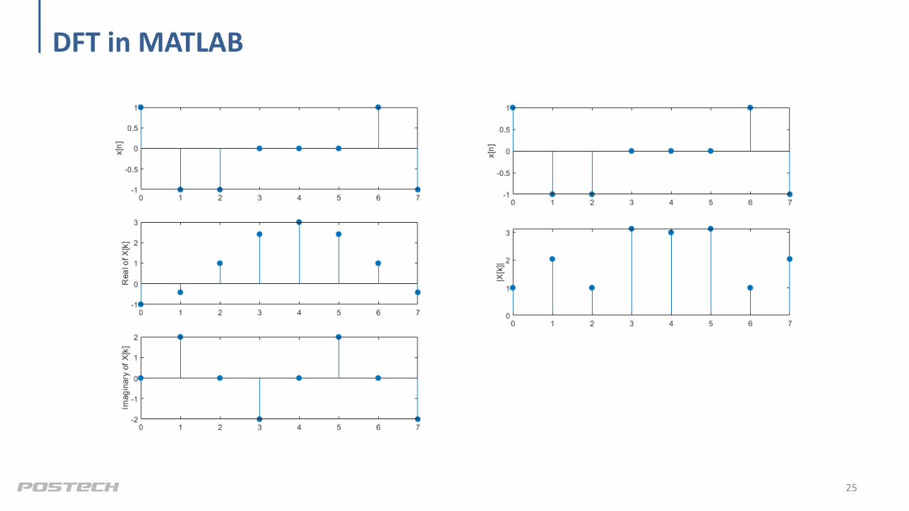
DFT in MATLAB

25

DFT Function

26

Example: DFT

27

Example: DFT

28

Example: DFT

29

Example: DFT

30

Fast Fourier Transform (FFT)

• FFT algorithms are so commonly employed to compute DFT that the term 'FFT' is often used to mean 'DFT'

– The FFT has been called the "most important computational algorithm of our generation"

– It uses the dynamic programming algorithm (or divide and conquer) to efficiently compute DFT.

• DFT refers to a mathematical transformation or function, whereas 'FFT' refers to a specific family of algorithms for computing DFTs.

– use fft command to compute dft

– fft (computationally efficient)

• We will use the embedded fft function without going too much into detail.

31

DFT Properties

• DFT pair

• DFT Frequencies

– 𝑋[𝑘] measures the similarity between the time signal 𝑥[𝑛] and the harmonic sinusoid 𝑠𝑘[𝑛]

– 𝑋[𝑘] measures the “frequency content” of 𝑥[𝑛] at frequency 𝜔𝑘 =2𝜋

𝑁𝑘

32

DFT Properties

• DFT and Circular Shift

– No amplitude changed

– Phase changed

33

DFT Properties

• DFT and Modulation

34

DFT Properties

• DFT and Circular Convolution

– Circular convolution in the time domain = multiplication in the frequency domain

• Proof

35

Filtering in Frequency Domain

36

• Circular convolution in the time domain = multiplication in the frequency domain

Example: Low-Pass Filter

37

Example: High-Pass Filter

38

Filtering in Time Domain

39

Filtering in Frequency Domain

40