Discrete Fourier Transform - Complex To Real

Chapter 5 - Discrete Fourier Transform (DFT)

ComplexToReal.com

Chapter 5

Discrete Fourier Transform, DFT and FFT

In the previous chapters we learned about Fourier series and the Fourier transform. These

representations can be used to both synthesize a variety of continuous and discrete-time

signals as well as understanding the frequency spectrum of the given signal whether periodic

or otherwise.

A majority of real life signals are discrete. Most are also aperiodic. They are also limited in

time. We never have an infinitely long signal, nor are most to the signals we deal with

perfectly periodic. Examples are stock market quotations, temperature measurement,

communications signals that carry voice, TV signals etc.. These are signals with a large

random component. Fourier opened the door to the analysis of these signals but at every step

some mathematical incongruity surfaced making necessary the development of the tool into

many different types.

So let’s look at our primary desire, which is that the input signal be discrete. For discrete

signals we can use the discrete Fourier series (DFS), but it is applicable only to periodic

signals. Or we can use the discrete-time Fourier Transform (DTFT), which is applicable to

non-periodic signals. The spectrum of the DFS is discrete whereas the spectrum of DTFT is

continuous. As a consequence of sampling, the output spectrums for both of these constructs

are periodic.

Fourier Transform(Aperiodic signals)Continuous time

CTFT

Fourier Transform(Aperiodic signals)

Discrete timeDTFT

Discrete Fourier Transform

(Periodic signals)Discrete time

DFT

Fourier Series(Periodic signals)

Discrete timeDTFS

Fourier Series(Periodic signals)Continuous time

CTFS

Same as one-period of discrete Fourier

series

Figure 5.1 – Relationship of various Fourier transforms

In the last chapter we arrived at DTFT, but DTFT falls short of an ideal analysis tool.

Yes, it applies to discrete time signals and to aperiodic signals. But the rub is that the DTFT

in frequency domain is continuous. Computer storage and calculation mode is inherently

discrete and DTFT is not an algorithm that can be computed using discrete (which means

essentially by computer) math. What we need is a combination of DFS which can be discrete

in frequency domain and the DTFT which is discrete in time domain. We saw that when we


ComplexToReal.com

compute a DTFT of a periodic signal, it is also discrete because this form of the DTFT is

same as sampled DFS coefficients. The results from the DTFT of periodic signals in Chapter

4 leads directly to the development of the Discrete Fourier Transform (DFT).

So we now move a new transform called the Discrete Fourier Transform (DFT). It

borrows elements from both the Fourier series and the Fourier transform. DFT was

developed after it became clear that our previous transforms fell a little short of what was

needed.

Let’s go through the path we took to get to the DFT. In the beginning there was continuous

time Fourier series. The input signal is periodic with period T and continuous in time, which

we don’t like. But CTFS gave us a discrete frequency spectrum which we do like.

Then we let the period go to infinity. This made the signal aperiodic which is something that

we also want, this we called the Continuous-time Fourier transform (CTFT). CTFT gave us a

discrete frequency spectrum, also good. But continuous time is still a problem and we want

to avoid dealing with it.

Then we sample the signal, get a discrete version of the signal and calculate the discrete-time

Fourier series (DTFS). The DTFS gives discrete frequency spectrum but unfortunately the

spectrum replicates.

Again by letting the period go to infinity we get the discrete-time Fourier Transform (DTFT).

This gives us a continuous frequency spectrum, which is not desirable. But we notice that if

take the DTFT of a periodic signal, which has the effect of limiting the signal to a time

window, the spectrum becomes discrete. This gives us the idea for the next development in

the series, the Discrete Fourier Transform (DFT), the topic of this chapter.

Input is Output Spectrum is

Periodic Time

Resolution

Periodic Frequency

Resolution

Fourier Series

Continuous

CT-DFS

Periodic Continuous No Discrete

Fourier Series

Discrete

DT-DFS

Periodic Discrete Periodic Discrete

Fourier Transform

CTFT

Non-periodic Continuous Non-

periodic

Continuous

Fourier Transform

DTFT

Non-periodic Discrete Periodic Continuous

Discrete Fourier

Transform

DFT

Non-periodic Discrete Periodic Discrete

Table I – Properties of Fourier transform input and output signals


ComplexToReal.com

Taking this further we present now the Discrete Fourier transform (DFT) which has all three

desired properties. It applies to discrete signals which may be

(a) Periodic or non-periodic

(b) Of finite duration

(c) Have a discrete frequency spectrum

DFT is similar to both DTFS and DTFT. The differences between the DFT and DTFT and

DFS are subtle. So first let’s look at the definition for the DTFT.

( ) [ ] j k

k

X x k e DTFT

(1.1)

Notable here are an infinite number of harmonics used in the calculation of the DTFT. And

because there are an infinite number of harmonics, resolution is infinitesimally small and

hence the spectrum of the DTFT is continuous.

The DFT is essentially a discrete version of the DTFT. It is a function of the frequency index

n, where the nth harmonic of the DTFT 2 nNn for 0 1n N . Here N is the period of

the signal. To derive the expression of the DFT, we substitute this value of the harmonic into

the DTFT equation (1.1). This is given by the following expression.

1

(2 / )

0

( ) [ ]N

j kn N

k

X n x k e DFT

(1.2)

The inverse DFT is given by

1

(2 / )

0

1[ ] [ ]

Nj kn N

k

x k X n e IDFTN

(1.3)

Here k is the time index, N the number of harmonics and r is the index of these, so that n/N is

the nth harmonic. We note that the only thing different between the DTFT expression (1.1)

and the DFT (1.2) is the range of summation. The DFT takes place over N points. The DFT

uses only a finite number of harmonics, instead of the infinite for the DTFT, namely N, so its

spectrum resolution as measured by the fundamental frequency 20 N

is discrete and finite.

Hence this expression gives a spectrum that is discrete. Of course we can pick a very large N,

but that does not change the fact that it is still a finite number and so the DFT output is

discrete. Conceptually speaking, it may be easier to think of the DFT as sampled DTFT at

specific frequency points.

In previous chapter, we calculated DTFTs by closed form analysis. DTFT of arbitrary signals

are often hard to calculate. DFT on the other hand lends itself to calculation by digital

devices. It has an easy to understand architecture as shown in Figure 1. It can be


ComplexToReal.com

implemented as a linear device with N inputs and N outputs. It is completely lossless and

bidirectional. N numbers go in and N numbers come out.

[0]x

[1]x

[ 1]x N

[2]x

[0]X

[1]X

[2]X

[ 1]X N

L data samples

21

0

[ ] [ ]N jn k

N

k

X n x k e

Use N out of L

Discrete Fourier Transform(DFT)

Figure 5.2 – Architecture of a DFT

[0]x

[1]x

[ 1]x N

[2]x

[0]X

[1]X

[2]X

[ 1]X N

21

0

1[ ] [ ]

N jn kN

k

x k X n eN

InverseDiscrete Fourier Transform

(DFT)

Figure 5.3 – Inverse Discrete Fourier Transform

The input to the inverse DFT are the N frequency domain samples. Let’s compare this to the

inverse expression for the DFS (Eq. 1.17, Chapter 3)

0

0

1

0

[ ]K

jn k

n

k

x k D e IDFS

(1.4)

The two equations (1.4) and (1.3) are very similar, with only a scaling difference. The

coefficients nD from the DFS are same as the transform X[n] in (1.4) The range is also same

as N samples. So we see how the DFT is a hybrid transform that is like the both the DTFT

and the DFS. It is very nearly identical to the DFS if we think of it as looking through an

observation window one period long and choosing to ignore what is outside that window.

DFT spectrum also repeats but because we limit the range to just 2 , calculations are limited

to just one main part which is sometimes also called the principal alias. But the true spectrum


ComplexToReal.com

does have all the other aliases besides the principal one located at the zero, as well all the

others we have to account for.

The difference between the DFT and its inverse IDFT is just a scaling term in the front of the

IDFT and a change of the sign of the exponent. The two expressions are very similar and

this makes the hardware/software implementation of DFT algorithm easy. You can easily do

it in Matlab with just one or two lines.

Matrix method for computing DFT

We can also view the DFT as a linear input/output processor consisting of N equations.

Assume we have collected L data symbols, then we need to make a decision about how long

the N as specified for the DFT processor should be. If N is less than L, then we select N

samples out of the L and perform the DFT calculations on these N points. If we choose N

that is larger than the L collected samples, then we have to perform some sort interpolation to

increase the number of samples from L to N. Some algorithms of the DFT will automatically

add a bunch of zeros to make the length N you have specified.

The exponential is kind of hard to type, so let’s make this substitution.

2 /j N

Ne W

And also this

2

2N

nkjn k nkN

N

je e W (1.5)

Remember to think of NW as a single complex exponential of frequency 2N

. Hence nkNW is a

matrix of several exponentials with both n and k ranging from 0 to N. Now rewrite the DFT

using this form.

0

[ ] [ ]N

k

nkX n x k WN

(1.6)

The index N indicates that this complex number is based on period N. Now we write Eq.(1.6)

in matrix form as

nkNWX x (1.7)

X is the output Fourier transform vector of size N and x is the input vector of same size.


ComplexToReal.com

[0] [0]

[1] [1]

[ 1] [ 1]

X x

X x

X N x N

X x (1.8)

The nkNW term in Eq. (1.6) is called the DFT matrix and is given by

2 1

2( 1)2

2( 1)1

4

( 1)( 1)

1 1 1 1

1

1

1

1 N

nkN N

n nN

NN N

NN N

nNN N n k

W

W W

W W

W

W W W

W

Note that the exponent of NW is the product of n and k. The matrix size is n by k, but since

both n and k are equal to, the size is also equal to N x N. The rows represent the index n of

the harmonics and columns the index k, time. The first row has index n = 0, so all the first

row terms are equal to 1, because

0)0( 01

j kkNnW e .

The first column has index k = 0, hence all nkNW terms in the first column have a zero

exponent and so all are also equal to 1. The second row, second term is equal to ( 1)( 1)n kN NW W and the rest can be understood the same way. Note that the matrix is

symmetrical about the right diagonal such that

TN NW W

We can also show that the inverse of this matrix is just the inverse of the individual terms.

1 *1N NW W

N (1.9)

We will call nkNW the DFT Matrix.

Let’s write out the DFT matrix for N = 4. If N = 4, then the product of n and k is also equal

to 4 x 4 = 16. To calculate the individual terms of the DFT Matrix nkNW , we need to recall the

following property of the complex exponential from Chapter 2.

N is equal to 4, so the fundamental frequency is equal to 20 4

.


ComplexToReal.com

2

4

4

2 2cos sin

j nknk

nk

W e

nk j nk

j

(1.10)

For all nk, a product which is always an integer, the cosine of 2nk is always zero. Sine

however is always equal to 1. So we get the various values of the matrix

41, 0 1

41, 1

41, 2 1

41, 3

4

nknkW j

n kW

n kW j

n kW

n kW j

From this we can develop the 4nkW matrix as

4

1 1 1 1

1 1

1 1 1 1

1 1

j jW

j j

(1.11)

The inverse comes easily from Eq. (1.9)

1 1 1 1

1 1

1 1 1 1

1 1

N

j jInverseW

j j

Notice that only the imaginary components changed sign. For this you have to remember

what matrix W is. Each term is a complex exponential. For the forward transform we need

0j n ke and for the reverse we need 0j n k

e . The difference between these is that the

imaginary part changes sign. cos sinj vs. cos sinj . So here you are seeing the

imaginary part changing sign for the inverse but not the real part.

We can now use this DFT matrix to calculate the DFT of any arbitrary signal of 4 input

points using the equation of (1.7). Larger DFT matrices would be needed to compute larger

size DFT.

Now we will revisit ideas some elementary signals and their DTFT and the DFTs.


ComplexToReal.com

DFT of Important functions

DFT of a delta function at the origin

Here we have a sequence of just one impulse at the origin. We already know that the DTFT

of an impulse is a constant 1. The DFT however is a train of impulses of amplitude 1.

Figure 5.4 – (a) Single impulse function at origin, (b) its Discrete Fourier Transform

(DFT) (c) its discrete-time Fourier Transform (DTFT)

If the DTFT of an impulse is a constant, then for the DFT, how did we go from a constant of

1 to a train of impulses? The reason is this. DFT is essentially the sampled version of the

DTFT. If the DTFT is a constant 1, then for DFT, we sample the DTFT at each of the DFT

harmonics which are every 4 . From the sifting property of delta function, we get 8 samples

which are called the principal alias, as we see in Fig. 5.4(b). Thereafter they repeat again

and hence we get an infinite pulse train.

This idea that the spectrum repeats every 2 is a key point which you will see repeated often

in this chapter. The inverse DFT or the IDFT of an impulse train will of course then be a

single impulse.

DFT/DTFT of a constant

Conversely if we have a time domain signal that is constant of amplitude 1, its DTFT is given

as

2 2m

X m (1.12)

This is a pulse train of magnitude 2 . The DFT of this case is exactly the same as the DTFT.

0 2 4 60

0.5

1

0 2 4 60

0.5

1

-5 0 5 10 15 200

0.5

1

1.5

2


ComplexToReal.com

0 3-2 -1 1 2

1

0 32 4-2-4

............2

Figure 5.5 – DFT of a constant function is same an impulse train.

DFT of a sinusoid

Here is a cosine of frequency 4 Hz of amplitude 0.7. The sampling frequency is 20 Hz. In (b)

we plot its spectrum which gives us two impulses of half the amplitude located at 4 Hz from

the origin, just as we would expect. The third figure shows the full DFT spectrum. The center

part is called the principal alias, thereafter the same repeats with the sampling frequency of

20 Hz. Note that the second set is centered at 20 Hz on the high side at -20 Hz on the low

side. These repeat at -40, -60 etc. the integer multiple of the sampling frequency.

(a)The sampled cosine signal (b)The spectrum of the cosine

(c)Repeating DFT

Figure 5.6 – The DFT of a cosine. (a) Time domain signal, (b) The DFT showing only

the principal alias, (c) the repeating DFT

The DTFT of this signal is given as

0 02 2

k k

X m m

(1.13)

The DTFT of a cosine is discrete and so is the DFT.

DFT of a complex exponential

0 5 10 15 20-1

0

1

-10 -5 0 5 100

0.2

-40 -20 0 20 400

0.2

0.4


ComplexToReal.com

This example shows the DFT of the sum of two complex exponentials of frequencies 4 and 6

Hz. We sample the signal with a sampling frequency of 32 Hz, which is of course much

bigger than minimum needed (12 Hz.)

1 2

1 2

[ ] 0.5 exp( 2 / ) 0.3exp( 2 / )

6, 4, 32s s

s

x k j f k F j f k F

f f F

The DFT of this signal are two impulses one at -6 Hz of amplitude .5 and the other at 4 Hz of

amplitude .3, which you already know. The set around the origin is the principal alias and the

rest are repetitions centered at 32 Hz from the origin.

Figure 5.7 – The spectrum of a complex exponential is just a single impulse at the

frequency of the exponential (a) The DFT showing only the principal alias, (c) the

repeating DFT

The DTFT of a complex exponential is given by

02 ( 2 )

k

X m

(1.14)

This is quite similar to the DTFT/DFT of a cosine, but of course, there is only one impulse

instead of two and it also repeats every 2 .

Properties of DTFT/DFT

We will go over properties of both DTFT and DFT in this section. DFT derives its properties

from both DFS and DTFT.

Periodicity: Repeating spectrum

The DTFT of a signal is periodic with 2 . The same is true for DFT.

[ ] [ 2 ]X X (1.15)

Most calculations of the DFT, be they done in closed form, software, hardware or Matlab etc.

show only the principal alias, the DFT actually consists of an infinity of the repeating

spectrum. Hence, in frequency domain, for signal processing purposes, we often have to filter

out the principal alias from all the others.

-20 -10 0 100

0.5

-40 -20 0 20 400

0.5


ComplexToReal.com

Time shifting: DFT of a delayed delta function

In this example, we show the effect of time shift in time domain on the DFT. Take a single

impulse which is displaced or delayed from the origin by one sample. The signal length is 16

samples but for this example, the length does not matter.

Figure 5.8 - A delayed impulse function

We calculate the DFT of this signal by

0

1

0

( ) [ ]N

jn k

k

X n x k e

What is 0 in the DFT equation? It is 216 8

because we have N = 16 samples in the signal,

although only one is non-zero.

What is x[k]?

It is [0 1 0 0 0 0 0 0 0 0 0 0 0 0 0 0 0] or we can say it is [ ] [ 1]x k k .

0

0

1

0

15

0

( ) [ ]

[ 1]

Njn k

k

jn k

k

X x k e

k e

The index k has disappeared in the last step because its value is equal to 1 from the delta

function. The DFT of an un-delayed delta function was a train of constant impulses but here

we are getting a complex exponential. The frequency of this exponential is 1 Hz, because the

signal goes through one cycle or 2 in 16 samples. This is not very obvious if we look at the

DFT. We don’t see the 1 Hz. But note that n is the sample number. There are 16 samples.

The fundamental frequency which is not in Hz, but in radians per sample is / 8 .

0 5 10 150

0.5

1


ComplexToReal.com

8( )

(0) 1

(1) .92 .38

(2) .70 .70

(3) .38 .92

jnX n e

X

X j

X j

X j

Here we plot the real and imaginary parts of the DFT.

Figure 5.9 - (a) the Real part of the DFT, a cosine of 1 Hz, (b) the Imaginary part of the

DFT of the delayed delta function.

It may help instead to look at the magnitude and the phase, the most common way of looking

at the spectrum of a signal. The delay does not effect the magnitude at all. Only the phase

changes. In (b), we see that the phase is changing. It progresses / 8 radians per sample,

and we get 2 in 16 samples.

Figure 5.10 - (a) The magnitude of the DFT, (b) Phase of the DFT.

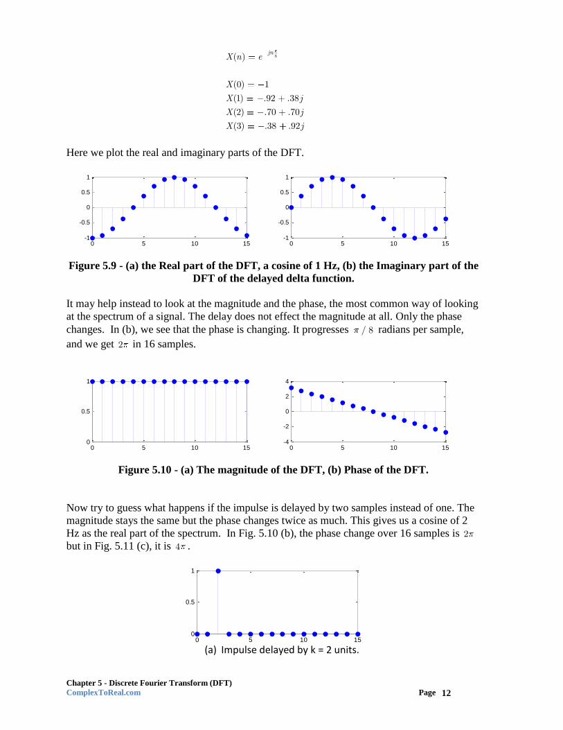
Now try to guess what happens if the impulse is delayed by two samples instead of one. The

magnitude stays the same but the phase changes twice as much. This gives us a cosine of 2

Hz as the real part of the spectrum. In Fig. 5.10 (b), the phase change over 16 samples is 2

but in Fig. 5.11 (c), it is 4 .

(a) Impulse delayed by k = 2 units.

0 5 10 15-1

-0.5

0

0.5

1

0 5 10 15-1

-0.5

0

0.5

1

0 5 10 150

0.5

1

0 5 10 15-4

-2

0

2

4

0 5 10 150

0.5

1


ComplexToReal.com

(b) The real part of the signal (a cosine of frequency 2 Hz.) (c) The phase

Figure 5.11 – (a) Impulse function delayed by 0k units, (b) the Real part of its DFT

shows increasing frequency (c) Phase similarly also increases at twice the speed as case

with one time unit delay.

These results show the shifting property of the DFT same as DTFT and other Fourier

transforms. The DTFT of this delayed signal is given by

0j kX e (1.16)

And equivalently we can write that if a signal is delayed by k0 units, then its DTFT (and also

DFT) is multiplied by a complex exponential of 0k . For the DFT, this is equal to 02k

N.

00[ ] [ ] j kex k k X n (1.17)

How does the delay turn into a frequency/phase shift? To understand what the delay means,

look carefully at the complex exponential multiplier. We are multiplying frequency by an

integer, k0. What is this frequency? Okay, this gets confusing here. Think of this term as an

exponential of frequency k0, and not . The term is not actually frequency here. As we

said earlier, it is measured as radians per sample, so it is not frequency per say in Hz. The

only way you know it is 1 Hz frequency is by noting the phase changes 2 over the period

and that makes the frequency 1 Hz. We know this indirectly. So it is a frequency of 1 Hz

(although the digital frequency is equal to / 8 ) for k0 = 1 and as you step through n, you

just trace out the sinusoid as shown below. This is why this phase shift is not a function of

the N, the size of the DFT.

0 5 10 15-1

-0.5

0

0.5

1

0 5 10 15-4

-2

0

2

4


ComplexToReal.com

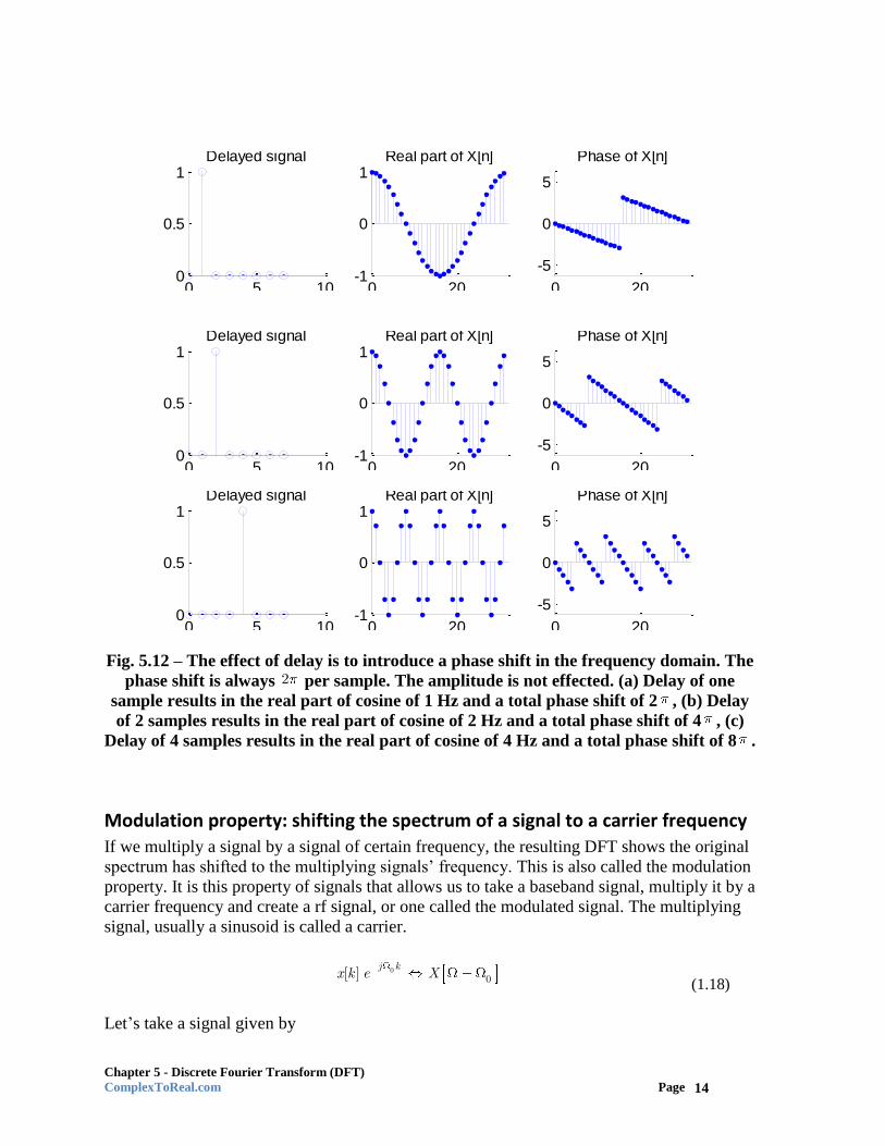
Fig. 5.12 – The effect of delay is to introduce a phase shift in the frequency domain. The

phase shift is always 2 per sample. The amplitude is not effected. (a) Delay of one

sample results in the real part of cosine of 1 Hz and a total phase shift of 2 , (b) Delay

of 2 samples results in the real part of cosine of 2 Hz and a total phase shift of 4 , (c)

Delay of 4 samples results in the real part of cosine of 4 Hz and a total phase shift of 8 .

Modulation property: shifting the spectrum of a signal to a carrier frequency If we multiply a signal by a signal of certain frequency, the resulting DFT shows the original

spectrum has shifted to the multiplying signals’ frequency. This is also called the modulation

property. It is this property of signals that allows us to take a baseband signal, multiply it by a

carrier frequency and create a rf signal, or one called the modulated signal. The multiplying

signal, usually a sinusoid is called a carrier.

0

0[ ]j k

x k e X (1.18)

Let’s take a signal given by

0 5 100

0.5

1Delayed signal

0 20-1

0

1Real part of X[n]

0 20

-5

0

5

Phase of X[n]

0 5 100

0.5

1Delayed signal

0 20-1

0

1Real part of X[n]

0 20

-5

0

5

Phase of X[n]

0 5 100

0.5

1Delayed signal

0 20-1

0

1Real part of X[n]

0 20

-5

0

5

Phase of X[n]


ComplexToReal.com

1 2

1 1

[ ] cos(2 / ) 0.7 cos(2 / )

1, 4, 30 50s s

s

x k f k F f k F

f f F or

First we compute the DFT of this signal. It has two impulses, one of magnitude 0.5 and the

second of 0.35. These are shown in (c). This signal is then multiplied by a carrier signal of

frequency 10 Hz to modulate it. The DFT of the modulating signal which is a single

frequency sinusoid, is given by two impulses located the frequency of the sinusoid as in (d).

Fig 5.13 – (a) the continuous signal, (b) Sampled signal with Fs = 30, (c) the spectrum of

the baseband signal of (b). It spectrum is located at the origin, (d) the DFT of the

carrier signal of frequency 10 Hz. (e) The spectrum of same signal after it is multiplied

by a carrier signal of frequency 10 Hz. (f) Same signal sampled with Fs = 50, which

increases the distance between the copies.

In Fig. 5.13 (e) we see just the principal alias of the spectrum when the signal is sampled at

30 Hz. The edges are samples 15, -16. The spectrum which was centered at origin, is now

replicated on each carrier frequency and is now located at 10Hz. Figure (f) shows the DFT

with additional copies of the spectrum. When the signal is sampled with Fs = 50 Hz. The

principal alias did not change, but the distance between the principal alias and the copies has

increased. Each copy is centered at integer multiple of 50 Hz.

Note when we sampled the signal at 30 hz, due to the 10 Hz shift, the 4 Hz component on left

is now at 14 Hz on the right, the edge of the principal alias. When we see the replicated

spectrum, note that next copy of the spectrum is very close to the principal alias because its

right edge is at 16 Hz. The same signal if it is sampled with a sampling frequency of 50 Hz,

moves the next copy of the spectrum to 50 Hz and hence we see larger distances between the

copies. This makes filtering less of a problem, we won’t need such a sharp filter.

0 1 2 3-2

-1

0

1

0 10 20 30-2

-1

0

1

-10 0 100

0.5

-20 -10 0 10 200

0.5

-10 0 100

0.2

-50 0 500

0.1

0.2


ComplexToReal.com

Figure 5.14 – Increasing the sampling frequency moves the copies of the spectrum

further apart

DFT of square-pattern pulses

Now let’s look at another class of signals, ones that are a discrete version of a square pulse.

The first pulse consists of four samples and the rest 28 are zeros for a total of 32 samples. We

write the DFT equation as

0

316 8 16

1

0

20 32

16 16 2 16 31

1

[ ] [ ] [ 1] [ 2] [ 3]

1

1

[0] 0.0313 + 0.0129j

[1] 0.0326 + 0.0032j

[2] 0.0261 - 0.0052j

[3] 0.0136 - 0.0073

Nj n k

N

k

j n j n j n

N

jn jn jn

N

X k k k k e

e e e

e e e

X

X

X

X

j

etc.

We see the magnitude of the spectrum plotted in Figure 5.15. Note that magnitude has a Diric

function pattern and not sinc. The width of the main lobe is equal to 2N/K, if N is the total

length and K the length of the non-zero pulses. In the first case below, N = 32, so we see that

the width of the main lobe is equal to 64/4 = 16 samples.

-50 0 500

0.1

0.2

0.3

-100 -50 0 50 1000

0.1

0.2

0.3

0.4


ComplexToReal.com

(a) Four impulses representing a square

(b) Square pulse length = 8 samples

(c) Square pulse length = 16 samples

(d) Square pulse length = 24 samples

(e) Square pulse length = 30 samples

0 5 10 15 20 25 30 350

0.5

1

0 5 10 15 20 25 30 350

1

2

3

4

0 5 10 15 20 25 30 350

0.5

1

0 5 10 15 20 25 30 350

2

4

6

8

0 5 10 15 20 25 30 350

0.5

1

0 5 10 15 20 25 30 350

5

10

15

20

0 5 10 15 20 25 30 350

0.5

1

0 5 10 15 20 25 30 350

10

20

30

0 5 10 15 20 25 30 350

0.5

1

0 5 10 15 20 25 30 350

10

20

30


ComplexToReal.com

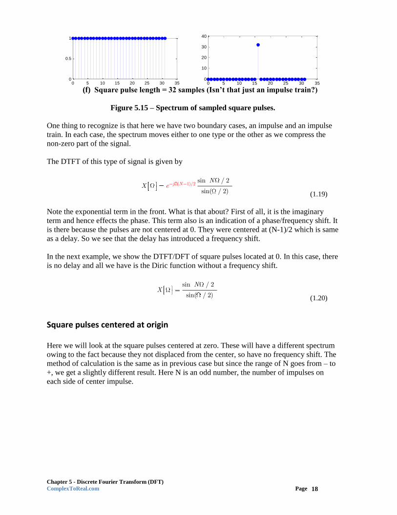
(f) Square pulse length = 32 samples (Isn’t that just an impulse train?)

Figure 5.15 – Spectrum of sampled square pulses.

One thing to recognize is that here we have two boundary cases, an impulse and an impulse

train. In each case, the spectrum moves either to one type or the other as we compress the

non-zero part of the signal.

The DTFT of this type of signal is given by

( 1)/2sin / 2

sin( / 2)j Ne

NX

(1.19)

Note the exponential term in the front. What is that about? First of all, it is the imaginary

term and hence effects the phase. This term also is an indication of a phase/frequency shift. It

is there because the pulses are not centered at 0. They were centered at (N-1)/2 which is same

as a delay. So we see that the delay has introduced a frequency shift.

In the next example, we show the DTFT/DFT of square pulses located at 0. In this case, there

is no delay and all we have is the Diric function without a frequency shift.

sin / 2

sin( / 2)

NX

(1.20)

Square pulses centered at origin

Here we will look at the square pulses centered at zero. These will have a different spectrum

owing to the fact because they not displaced from the center, so have no frequency shift. The

method of calculation is the same as in previous case but since the range of N goes from – to

+, we get a slightly different result. Here N is an odd number, the number of impulses on

each side of center impulse.

0 5 10 15 20 25 30 350

0.5

1

0 5 10 15 20 25 30 350

10

20

30

40


ComplexToReal.com

-4 0 3-3 -2 -1 1 2

1(a)[ ] 1x k k N

-4 0 3-3 -2 -1 1 2

1(b) 2N

3N

-4 0 3-3 -2 -1 1 2

1(c)

5N

Figure 5.16 - Sampled square pulse centered at zero.

Now let’s plot the DFT of this signal as given by the following formula.

0

1[ ]

0

k Nx k

N k K

Also

0[ ] [ ]x k x k K the signal is periodic.

00

0

0

0

(2 1)

(2 1)sin

1

1sin

n

Nk lK

KN

nCK

elsewhereK

nK

(1.21)

DFT is the repeating version of these coefficients given by

0

2[ ] 2 n

k

nX C

K (1.22)


ComplexToReal.com

5N

2N

3N

-5

0

5

-3 -2 - 0 2 3

0

5

10

-3 -2 - 0 2 3

0

5

10

-3 -2 - 0 2 3

Figure 5.17 – Spectrums of square pulse centered at zero.

Here we have plotted the DTFT along with DFT. As we increase N, the size of the square

pulse gets bigger so are we not approaching an impulse train again? The spectrum also

approaches impulses since the lobes are getting narrower which is the spectrum of an impulse

train.

Sinc function as an input signal

When the input is a sinc function, such as

[ ] sincW Wk

x k (1.23)

Then its DTFT is given as

1

0 2

WX

W (1.24)


ComplexToReal.com

In theory, the sinc signal would give a perfectly flat top-hat like spectrum as shown in Fg. 5-.

Figure 5.18 – A sinc pulse of infinite length has a top-hat like DTFT.

But this does not happen if you employ the DFT. The reason is that the sinc function is

infinitely long and when we truncate it to compute the DFT, we get what is called ringing

(also called leakage). Since we can never get an infinitely long signal, the spectrum of a

truncated sinc function will always show this pattern, This is shown in Fig. 5.19. And in (b)

and (d), same spectrum plotted in stem and the in classical fashion by connecting the values.

Figure 5.19 – The DFT of a since function that has been truncated to four lobes on each

side.

The actual spectrum of course repeats with sampling frequency. Here we see the square

pulses located at -64 and +64 Hz which is the sampling frequency of this signal. Notice that

each “square” pulse is centered at integer multiple of the sampling frequency.

-5 0 5

-0.2

0

0.2

0.4

0.6

0.8

TIME, seconds

sin(2 0.5 t)/(2 0.5 t)

AM

PL

ITU

DE

-1 0 10

0.5

1

1.5

FREQUENCY,Hz

MA

GN

ITU

DE

0 10 20-0.5

0

0.5

1

TIME, seconds

AM

PL

ITU

DE

-20 0 200

0.5

1

1.5

FREQUENCY, HZ

MA

GN

ITU

DE

0 10 20-0.5

0

0.5

1

TIME, seconds

AM

PL

ITU

DE

-20 0 200

0.5

1

1.5

FREQUENCY, HZ

MA

GN

ITU

DE


ComplexToReal.com

Figure 5.20 – When sampled with Fs = 64, the spectrum repeats with same frequency.

Time scaling: Effect of oversampling and downsampling

In 5.21 (a) we see a signal of 4 samples. Its DFT is shown in (b). Now we stretch this signal

by inserting a zero in between each sample. The effect of this oversampling is actually

surprising. The oversampling by a factor k, results in the spectrum replicating k times. We

see this in (e) and (f).

(a) Initial signal (d) Spectrum of initial signal

(b) Signal upsampled by 2 (e) Spectrum repeats

(c) Initial signal upsampled by 5 (f) Spectrum repeats five times

Figure 5.21 – Effect of oversampling

Here is an another example. Let’s take the square pulse centered at origin with N = 3. We get

the following signal and its DFT. When we oversample this signal and insert 2 zeros between

-100 -50 0 50 1000

0.5

1

1.5

0 1 2 30

0.5

1

0 1 2 30

1

2

0 2 4 60

0.5

1

0 2 4 60

1

2

0 5 10 15 200

0.5

1

0 5 10 15 200

1

2


ComplexToReal.com

each sample, we see the following spectrum. The spectrum repeats by the factor of

oversampling.

Figure 5.22 – Effect of oversampling on a square pulse

Down-sampling the oversampled signal by the same amount, will return the signal to its un-

stretched configuration, both in time and frequency domain. Try it with the Matlab code.

Zero-padding

In figure 5.22, we show that the signal size is 16 points, however the DFT size is 128 points.

The extras points come as additional zeros appended to the signal. The appended points

reduce the frequency resolution by the relationship 2

N. As N gets larger, the resolution get

smaller and we get a better defined spectrum such as we can see. Zero padding can only be

done at the end or at the start of the signal. It will not provide any additional information as

information is a function of the sampling frequency and not the size of the DFT.

Example 5-1

To compute the DFT of an arbitrary signal, we will now use both the closed solution first and

then use the metric method. The signal in Fig. 5.16 is given as

[ ] [ ] .5 [ 6]x k k k

0 5 10 150

0.5

1

0 50 100

0

2

4

0 5 10 150

0.5

1

0 50 100

0

2

4

0 5 10 150

0.5

1

0 50 100

0

2

4


ComplexToReal.com

Figure 5.23 – Time domain signal of example problem 5-2

Signal length is: L = 8. Taking DFT of a series of impulses can be pretty easy. First we

determine the fundamental frequency of this signal. N = 8 and so 2 20 8 4N

. This is a

good resolution because of both the non-zero impulses fall on one of the bins which are

separated by

4k

Let’s compute the DFT of the signal as

2

28

28

1

07

07

0

[ ] [ ]

[ ]

[ ] .5 [ 6]

N

Nj n k

k

j n k

k

j n k

k

X n x k e

x k e

k k e

In the last step, the multiplication of the complex exponential by a delta function just means

that we grab the value of the exponential at the location of the delta function which we do

here for k = 0 and k = 6.

2 28 8

2 28 8

28

0 66

[ ] .5 [ 6]

.5

1 .5

j n k j n k

j n k j n k

k kj n

k e k e

e e

e

Now we finish the job, noting that index k is gone.

28

32

76

0

[ ] 1 .5

1 .5

j n

k

j n

X n e

e

(1.25)

Now take a careful look at this. Is this not just the amplitudes of the two impulse functions,

one at 0 and the other at n = 6. We have to actually go through each k and determine the

values of the DFT for each n. These are given by

0 2 4 60

0.5

1


ComplexToReal.com

32

32

3

4.5

6

7.5

9

11.5

[ ] 1 .5

[0] 1.5

[1] 1 .5 1.0 + 0.5j

[2] 1 .5 0.5

[3] 1 .5 1.0 - 0.5j

[4] 1 .5 1.5

[5] 1 .5 1.0 + 0.5j

[6] 1 .5 0.5

[7] 1 .5 1.0 - 0.5j

j n

j

j

j

j

j

j

j

X e

X

X e

X e

X e

X e

X e

X e

X e

(a) The magnitude of the spectrum

(b) The phase of the spectrum

Figure 5.24 – Spectrum of signal of example 5-1

20 .5 32 1.5

Figure 5.25 – Magnitude spectrum of signal of example 5-1. Note it repeats what is

shown in Fig. 5.18 (a)

We did the analysis for 8 points. Now we will do exactly the same thing first for 7 points and

then for 128 points by padding the end of the signal with a lot of zeros.

0 1 2 3 4 5 6 70

0.5

1

1.5

0 1 2 3 4 5 6 7-0.5

0

0.5

0 2 4 60

0.5

1

0 2 4 60

1

2


ComplexToReal.com

Figure 5.26 DFT of a signal with different amounts of zero padding, size = 7, size = 8,

size = 128

So zero padding gives more points of interpolation. However, is the signal contained a higher

frequency signal beyond the twice sampling frequency, zero-padding would do nothing to

help discover it.

Example 5-2

Find the DFT of sequence

2 2[ ] 1 cos 0,1, 7

8

kx k k

Its easier to convert the sinusoid into complex exponentials. So we write

22 2 2 2

8 8 4 41 3 1 1[ ] 1

4 2 4 4

k k k kj j j j

x k e e e e

The DFT coefficients are;

30

2[0] 2 2,6

0

n

X n

else

0 10 20 300

0.5

1

0 10 20 300

1

2

0 20 40 600

0.5

1

0 20 40 600

1

2

0 50 1000

0.5

1

0 50 1000

1

2


ComplexToReal.com

Example 5-3

Find the sequence [ ]y k that has for its DFT 2

212[ ] [ ]

j nY n e X n , given that

[ ] ( ) 2 ( 6)x k k n and [ ]X k is the 12 point DFT of [ ].x k

The DFT of [ ]x k is equal to

26

12[ ] 1 2 1 2( 1)j n

nX n e

Multiplication of this DFT by a complex exponential has the effect of delaying the signal in

time domain. So [ ]y k is a delayed form of [ ].x k The delay operator is

26

12je

The delay is 0 6k , hence [ ]y k is given by

12[ ] [ 2] 2 4 10y k x k

Example 5-4 Compute the DFT of the aperiodic signal given by the following four samples.

X[k] = [ 2 1 -3 4]

We write its DFT by observation like this.

3

/2 3 /2

0

2 1 3 4j n j n j n

n

e e e

From here we can compute the first two terms as

/2 3 /2

[0] 2 1 3 4 4

[1] 2 3 4

2 3 4

5 3

j j j

X

X e e e

j j

j

Now we will use the matrix method for the solution to see if we get the same thing.

[ ] [2 1 3 4]x k


ComplexToReal.com

We write the matrix equation using the DFT matrix for N = 4.

[0] 1 1 1 1 [0]

[1] 1 1 [1]

[2] 1 1 1 1 [2]

[3] 1 1 [3]

1 1 1 1 2 4

1 1 1 5 3

1 1 1 1 3 6

1 1 4 5

X x

X j j x

X x

X j j x

j j j

j j 3j

Okay, we got the same thing!

Now let’s compute the inverse DFT.

1[ ] [ ]Nx k W X n

Here we will use the matrix we developed for the inverse DFT. Note that various sizes of the

DFT can be pre-computed and saved in the computer hence making computations easy for

any size B.

[0] 1 1 1 1 [0]

[1] 1 1 [1]

[2] 1 1 1 1 [2]

[3] 1 1 [3]

1 1 1 1 4 2

1 1 5 3 111 1 1 1 6 34

1 1 5 3 4

x X

x j j X

x X

x j j X

j j j

j j j

Example 5-5

A band-limited signal DFT is sampled at the rate of 100 Hz and is band-limited to 25 Hz.

The number of samples is N = 50.

(a) What is spectral spacing?

(b) What frequency is represented by n = 20 and 40?


ComplexToReal.com

The DFT is basically a set of sampled points at N frequencies. So each bin of 50 samples (the

size of the DFT) represents 2 Hz which is the spectral spacing. Bin 20 represents 40 Hz and

bin 40 represents 80 Hz.

What if this signal was sampled at the rate of 25 Hz instead of 100? What would be the value

of these bins then.

Sampling frequency of 25 Hz is less than the minimum rate (needs to be 50 Hz) and so we

will get aliasing. The spectral resolution is 0.5 Hz. For bin 20, we get 10 Hz, and 20 Hz for

bin 40. This is beyond the 12.5 Hz range of the DFT, so at bin 20 we will get aliased

adjacent spectrum value and the answer would not be correct.

Truncation effects

Let’s take this sampled cosine wave with period equal to N = 8.

Figure 5.27 – A sampled cosine wave with N = 8.

The DFT of the signal should be pretty clear to you by now. It consists of just two impulses

located at the positive and negative frequency of the signal centered at the origin.

To do the DFT of this signal, how many points do we need? This is a crucial point. The

signal repeats every 8 samples. So we need at least 8, anything more is extra and may or may

not be helpful, as we will see.

Assume that we are going to use some part of the above sampled cosine signal, which we

obtain by multiplying this signal with a “window”, a constant signal of a certain length. For

example, if we wanted just one period, the window would be 8 samples long and would have

an amplitude of 1.0 . So the N-sample segment of the signal is equivalent to the input signal

times a window function of length N. We call the resulting “truncated” signal a windowed

signal.

( ) ( ) ( )wx m w m x m

We define the window function as a rectangular function given by

1 0 1

( )0

m Nw m

otherwise (1.26)

0 10 20 30 40 50-1

0

1


ComplexToReal.com

Where M n M is the time length of the window. This window function is all ones. So

it is just a rectangular function over a certain number of samples, N. The truncated function

( )wx m now becomes a signal of finite duration. We can also think of this signal as

[ ]

( )0m

x n M n Mx m

otherwise (1.27)

Multiplying these two signals together is same as doing convolution in frequency domain, so

we can write the relationship of the spectrums as a convolution.

( ) ( ) * ( )wX k W k X k (1.28)

Our signal is a sinusoid and we know that its transforms looks something like this

0 0( ) ( ) ( )X (1.29)

The DTFT of the window function, which is a square pulse like function is a Diric (repeating

sinc) function.

1

22

2

sin( )

sin

Nj N

W e (1.30)

Figure 5.28 – The spectrum of the rectangular window.

This function is zero at all k integer values except at k = 0. It has a sinc-like shape and N-1

zero crossing. Now we compute the DTFT of the truncated signal by convolution of the two

transforms.

1

220 0

2

( ) ( ) * ( )

sin( ) ( ) *

sin

mN

j

X X W

Ne

(1.31)

0 50 100 150 200 250 300-0.02

0

0.02

0.04


ComplexToReal.com

If you look carefully you can figure out what this convolution will do. Procedures with delta

functions are fairly easy. So the first delta function copies the sinc function at and the

second delta function creates another copy at . these are superimposed and create a

smeared double peak spectrum as shown below.

Figure 5.29 – The DTFT and DFT of the windowed cosine.

The DTFT of the window function is shown in the red line. It is a continuous function. The

DFT however, is sampled values of this function, the 8 values in keeping with the original 8

sample data. If we did not plot the DTFT, all you would see are the two impulses and a

bunch of zeros, exactly what you would expect as the DFT of a cosine signal.

The figure below shows what happens if the window is 16 samples long. Notice that the

peaks are closer together. We sample this function at 16 places and again get a pretty decent

looking DFT. It’s a pure sinusoid, only the two impulses. Nothing else.

Figure 5.30 – The DTFT and DFT of the windowed cosine, with N = 256

But wait, let’s try a window of size of 12 instead of 8 samples. We again do a DFT of size

256 points.

0 50 100 150 200 250 3000

0.005

0.01

0.015

0.02

0 50 100 150 200 250 3000

0.01

0.02

0.03

0.04


ComplexToReal.com

Figure 5.31 – The DTFT and DFT of the windowed cosine, with window size = 12

samples, N = 256

Oh no, whatever happened to the clean looking DFT of Fig. 5.27. The DFT points now seem

to be at the peak of the side lobes not so in the main lobes. The larger number of points has

ended up ruining the form of the DFT. This one does not have two impulses and a bunch of

zeros as the previous two cases. The underlying signal is still the sinusoid, it did not change,

in fact, we gave the DFT more points, 12 vs. 8, so why are we getting this mish-mash?

Note that the DTFT has not changed, it looks the same as the one before, what has changed is

the place where we sample the DTFT, which is the DFT. This effect is due to the window

size and it has happened for one simple reason: the window size is not an integer multiple of

the signal period, N. The period of the signal is 8 but we have used 12 points of the signal.

Looking at the 12 points, in isolation, we see that if we string together the 12 samples of the

cosine, the pieces would not join at the end. The signal has lost its periodicity and hence its

DFT looks awry.

In reality, when we get a signal, we do not know the underlying signal period. We pick the

length of signal on which to do the analysis based on numerical convenience. So rectangular

windowing is a natural part of the problem of finite length signals. It not only truncates the

signal but also introduces discontinuities at the edges in most cases. Unless of course, we get

lucky and happen to pick a length that exactly matches an integer multiple of the signal

period. This is of course not likely. So what can we do? Do we have to accept a messed up

DFT? Well no, we can apply another window to the truncated signal, one that will reduce the

effect of the truncation (in reality the rectangular window.). So is there some other window

we could have used that would allow us to obtain a DFT that is closer to the real sinusoid

underneath? Yes, there are very many windows. We will discuss these in the next chapter.

Most of them work by forcing the edge points to zero, so the ends always match and we get a

forced periodic signal

DFT is something is generally done in software using the matrix method shown. Using the

general matrix method, it is possible to do a DFT of any size.

0 50 100 150 200 250 3000

0.005

0.01

0.015

0.02

0.025


ComplexToReal.com

Fast Fourier Transform (FFT)

The DFT although clear and easy to compute, requires a good many calculations. For each

harmonic, we have N+1 multiplications and we do this N times, giving us N2 + N

calculations. A 256 point DFT would require 65792 calculations. The algorithm for Fourier

Transform existed for more than 200 years before it came into widespread use mostly

because we could not cope with such large number of computations. The algorithm waited

for the development of the microprocessor.

In 1948, Cooley and Tukey and came up with a computational breakthrough called the Fast

Fourier Transform algorithm. This was an ingenious manipulation of the inherent symmetry

of the calculations. It now allowed the computation of a N point DFT as a function only 2N

instead of the N2. So a 256 point DFT would only require 512 calculations, a huge

improvement from 65792 calculations doing it the laborious way. The algorithm was quickly

and widely adopted and is the basis of all modern signal processing.

Most DSP books spend a lot of time going through the mechanism of the FFT and how it is

computed. Huge butterfly figures in our books help to confuse and confound us as to what is

actually going on. Most of us just give up on it. Let me alleviate your guilt. Although

extremely important in itself, the understanding of the mechanism of the FFT is not all that

important. So, I am skipping over the details of its implementation.

The method has been programmed in all sort of software and we can safely skip it without

impacting our understanding of the application of the DFT and the FFT. In Matlab, you can

do a FFT of any size. However in most hardware, efficiency is important so the FFT

algorithm (and there are several versions) is based on signal size which is of length N, such

that N is a number generated by.., with k an integer. We will assume that the implementation

is a black-box, into which we feed the data. As long you understand what this box is doing,

understanding how efficiently it is doing its job is not that important. Only a decade or so

ago, most hardware FFT size was limited to about 9000 points, with better hardware, the size

and speed are not a big limitation any more.

The main thing one needs to know about the FFT is that it works only with sample numbers

that are powers of 2, such as 16, 32, 64 etc. We cannot do a FFT on an arbitrary number of

samples as we can with DFT or FFT in Matlab, which is used mostly for didactic and

exploration purposes process. The FFT is a DFT with constraints on the number of input

samples.

The other thing about the FFT process to know is that it allows zero-padding. Let’s say we

have 28 samples and we wish to do a DFT via the FFT, we can do two things, 1. we can do a

16 point FFT and discard the remaining 12 points or we can insert four zeros at the end so we

have 32 points. Now we can do a 32 point FFT. The zero-padding provides us better

resolution but does not provide any extra information. The frequency detected is still a


ComplexToReal.com

function of the original N samples and not the zero-padded length, although the FFT does

look a lot better. And looks do count.

Charan Langton

Copyright 2013, All Rights reserved

www.complextoreal.com

Matlab Code

Program 1 %DFT of a cosine clf clear all t = 0: .01: 3; xc = 1*cos(2*pi*3*t); figure(1) plot(t, xc) fs = 21; k = 0: 20; xn = 1*cos(2*pi*3*k/fs); figure(2) stem(k, xn)

xf = (1/30)*(fft(xn,21)); n = -10: 10 figure(3) xf2 = abs(fftshift(xf,2)) stem(n, abs(fftshift(xf,2)), 'filled') xfm2 = [ xf2 xf2 xf2]; figure(41) n2 = -31: 31; stem(n2, abs(xfm2), 'filled')

Program 2 %complex exponential N = 32; n = 0: N-1; x = 0.3*exp(1i*2*pi*4*n/N)+ 0.5*exp(-1i*2*pi*6*n/N); ND = 32; xf = (1/32)*fft(x, ND); figure(1) n2 = -16: 15; xfs = abs(fftshift(xf,2)); stem(n2, xfs, 'filled') figure(2) x = [x zeros(1,ND-N)] stem(n2, real(x), 'filled') xfm2 = [ xfs xfs xfs]; figure(3)

http://www.complextoreal.com/


ComplexToReal.com

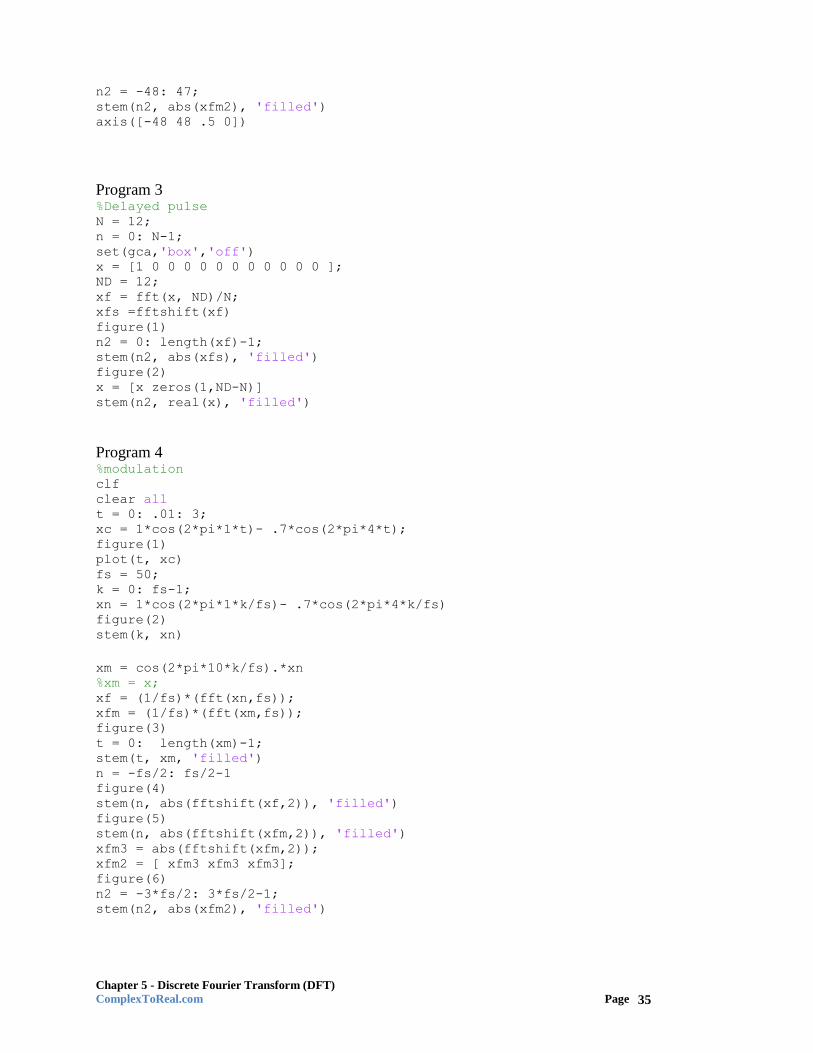
n2 = -48: 47; stem(n2, abs(xfm2), 'filled') axis([-48 48 .5 0])

Program 3 %Delayed pulse N = 12; n = 0: N-1; set(gca,'box','off') x = [1 0 0 0 0 0 0 0 0 0 0 0 ]; ND = 12; xf = fft(x, ND)/N; xfs =fftshift(xf) figure(1) n2 = 0: length(xf)-1; stem(n2, abs(xfs), 'filled') figure(2) x = [x zeros(1,ND-N)] stem(n2, real(x), 'filled')

Program 4 %modulation clf clear all t = 0: .01: 3; xc = 1*cos(2*pi*1*t)- .7*cos(2*pi*4*t); figure(1) plot(t, xc) fs = 50; k = 0: fs-1; xn = 1*cos(2*pi*1*k/fs)- .7*cos(2*pi*4*k/fs) figure(2) stem(k, xn)

xm = cos(2*pi*10*k/fs).*xn %xm = x; xf = (1/fs)*(fft(xn,fs)); xfm = (1/fs)*(fft(xm,fs)); figure(3) t = 0: length(xm)-1; stem(t, xm, 'filled') n = -fs/2: fs/2-1 figure(4) stem(n, abs(fftshift(xf,2)), 'filled') figure(5) stem(n, abs(fftshift(xfm,2)), 'filled') xfm3 = abs(fftshift(xfm,2)); xfm2 = [ xfm3 xfm3 xfm3]; figure(6) n2 = -3*fs/2: 3*fs/2-1; stem(n2, abs(xfm2), 'filled')


ComplexToReal.com

Program 5 %square pulse N = 32; x = ones(1,N); n = 0: length(x)-1; ND = 32; xf = fft(x, ND) xfs = fftshift(xf) figure(1) n2 = 0: length(xf)-1; stem(n2, abs(xfs), 'filled') figure(2) x = [x zeros(1,ND-N)] stem(n2, x, 'filled')

Program 6 T = 0.25; t = [0:T:(20-T)]'; N = length(t); shift = 40*ones(N,1);

y = sin (pi*t - pi*T*shift) ./ (pi*t - pi*T*shift); y(41)=1;

figure(2) subplot(1,2,1); plot(t,y) %title('x(t), T=0.25 & P=20 sec'); xlabel('TIME, seconds'); ylabel('AMPLITUDE') Y = T*fft(y); MY = abs(Y); fd = 1/(N*T); f = [0:fd:(N/2-1)*fd]'; f2 = (-(N/2): (N/2)-1); %mag2 = fftshift(MY,2); mag = MY(1:(N)/2); magt = mag(end:-1:1);

mag2 = cat(1, magt, mag); subplot(1,2,2); plot(f2, mag2) %stem(f2,mag2, 'marker', 'none') %title('MAGNITUDE SPECTRUM'); xlabel('FREQUENCY, HZ'); ylabel('MAGNITUDE') axis([-30 30 0 1.5])

Program 7 %DTFT and DFT of a window clf set(gca,'box','off') S = 12;% size of window n = 0: 47; %for showing time domain signal x = cos(2*pi*n/8); %the signal with N = 8 stem(n, x) figure (1) win = ones(1,S) % window of size S, al ones %win = [.1 .3 .5 1 1 .5 .3 .1]


ComplexToReal.com

N = S; xw =(1/N)* fft(x, N); s = 0: S-1; N2 = 256; winw = (1/N2)* fft(win, N2); %FFT of the window stem(s, xw) %fft of signal figure(2) n2 = 0: 255; plot(n2, (fftshift(winw))); %fft of window figure(3) sd = x(1:S) mult = sd.*win(1:S); %multiply two signals multw = (1/N2)* fft(mult, N2); %fft of both plot(n2, (fftshift(abs(multw))), '-.r'); hold on A = (fftshift(abs(multw))); tvar = 256/S; sd = A(1 : 256/S : end); n5 = 1: 256/S: 256; stem(n5, sd)

Discrete Fourier Transform - Complex To Real

Documents

Transcript of Discrete Fourier Transform - Complex To Real