Discrete exponential Bayesian networks: Definition, learning andapplication for density estimation$

Aida Jarraya a,b,n, Philippe Leray b, Afif Masmoudi a

a Laboratory of Probability and Statistics, Faculty of Sciences of Sfax, University of Sfax, Tunisiab LINA Computer Science Lab UMR 6241, Knowledge and Decision Team, University of Nantes, France

a r t i c l e i n f o

Article history:Received 20 November 2012Received in revised form15 May 2013Accepted 18 May 2013Available online 15 February 2014

Keywords:Exponential familyBayesian networkDensity estimation

a b s t r a c t

Our work aims at developing or expliciting bridges between Bayesian networks (BNs) and NaturalExponential Families, by proposing discrete exponential Bayesian networks as a generalization of usualdiscrete ones. We introduce a family of prior distributions which generalizes the Dirichlet prior appliedon discrete Bayesian networks, and then we determine the overall posterior distribution. Subsequently,we develop the Bayesian estimators of the parameters, and a new score function that extends theBayesian Dirichlet score for BN structure learning. Our goal is to determine empirically in which contextssome of our discrete exponential BNs (Poisson deBNs) can be an effective alternative to usual BNs fordensity estimation.

& 2014 Published by Elsevier B.V.

1. Introduction

Probabilistic graphical models, specifically Bayesian networksare tools for knowledge representation under uncertainty. Underusual hypotheses, the joint probability distribution associated to aBN is decomposed in the product of local conditional probabilitydistribution of each variable given its parents in the graph.

Some Bayesian estimation methods can be used in order toestimate the parameters of each conditional probability distribution,given one dataset and one a priori distribution over the parameters.The computation of the posterior distribution is useful for twopurposes: to estimate the probability of a graph given the data andthen to find the better graph (structure) that fits the data [6,17,16].

Reviewing the literature, we find abundant research and worksdealing with discrete Bayesian network, where the conditionaldistribution of each variable, given its parents, is a multinomialdistribution [28].

In this paper, we are interested in extending the distribution ofvariables to the natural exponential family (NEF) which represents avery important class of distributions in probability and statisticaltheory [2,24]. This idea has previously been developed by Bealand Ghahramani [3] (conjugate–exponential models) for Bayesian

networks with latent variables. They concentrated their work onvariational ExpectationMaximization (EM) estimation needed becauseof latent variables, but they did not clarify the Bayesian estimatorsused, hence restricting their experiments to the usual multinomialdistributions. Wainwright and Jordan [30] also proposed an interestingstudy of graphical models as exponential families, showing that veryspecific structures of directed or undirected probabilistic graphicalmodels can be interpreted as exponential distributions. Our workpursues with the same general idea, developing bridges between BNsand NEFs, dealing with discrete exponential BNs instead of usualmultinomial ones in order to explore a wider range of probabilisticmodels. We formally introduce a family of prior distributions valid forany NEF distribution and show that this family of priors generalizesthe Dirichlet prior used in discrete multinomial BNs. Then, we are ableto express the global posterior distribution and a new score functionfor learning the structure of any discrete exponential BN, and theBayesian estimators for parameters of such BNs. Our work aims todetermine empirically in which contexts one class of these discreteexponential Bayesian networks (Poisson deBNs) can be an effectivealternative to usual Bayesian networks for density estimation.

The present paper is structured as follows. In Section 2, wereview existing results for discrete multinomial BN learning. Afterthat, in Section 3, we review some of the properties of naturalexponential families with quadratic variance functions. In Section4, we propose our results concerning structure and parameterslearning for discrete exponential BNs. Section 5 aims at explicitingour experimental protocol, evaluation criteria, and gives an inter-pretations of results. Finally, we conclude with perspectives for afuture work.

Contents lists available at ScienceDirect

journal homepage: www.elsevier.com/locate/neucom

Neurocomputing

http://dx.doi.org/10.1016/j.neucom.2013.05.0610925-2312 & 2014 Published by Elsevier B.V.

☆This paper is an extended version of theoretical and experimental resultsinitially presented in [20,21].

n Corresponding author at: LINA Computer Science Lab UMR 6241, Knowledgeand Decision Team, University of Nantes, France.

E-mail addresses: aidajarraya@yahoo.fr (A. Jarraya),philippe.leray@univ-nantes.fr (P. Leray), Afif.Masmoudi@fss.rnu.tn (A. Masmoudi).

Neurocomputing 137 (2014) 142–149

2. Discrete Bayesian network background

2.1. General definition

Consider a finite set X ¼ fX1;…;Xng of random variables.A Bayesian network (BN) is a directed acyclic graph G and a setof conditional probability distributions which represent a jointprobability distribution

PðX1;…;XnÞ ¼ ∏n

i ¼ 1PðXijpaiÞ ð1Þ

where pai represent the parents of node Xi in G.Bayesian networks allow to represent distributions compactly

and to construct efficient inference and learning algorithms.Distinct directed acyclic graphs may sometimes encode the sameset of independence relations and hence, may be considered asMarkov equivalent graphs.

In what follows, we assume that the local distributions dependon a finite set of parameters μ¼ ðμijÞ1r irn;1r jrqi , where qi is thenumber of parent configurations for variable Xi.

Usually, as described in [28], discrete Bayesian networksstudied in the literature assume that local conditional distributionsPðXijpaiÞ are multinomial distributions Multð1;μij1;…;μijri

Þ, i.e.multivariate Bernoulli distributions with parameters ðμij1;…;μijri

Þ.

2.2. Structure learning

Learning Bayesian network structure from dataset is a NP-hardproblem [5] and is still one of the most exciting challenges inmachine learning.

There are three classical approaches often used for BN structurelearning. First, constraint-based methods consist in detecting (in)dependencies between the variables by performing conditionalindependence tests on data. Second, score-and-search basedapproaches use a score function to evaluate the quality of a givenstructure and a heuristic to search in the solution space. The thirdhybrid approach merges the two previous approaches.

In previous works, Acid et al. [1], Brown et al. [4], Fu [11] andTsamardinos et al. [29] provide comparisons of Bayesian networklearning algorithms. Recently, Daly et al. [9] states that score-and-search approaches are some of the most successful strategies forlearning Bayesian networks. Even a simple heuristic such asgreedy search [6] can produce good results. The choice of thescoring function is also an open question. This function, oftenrelated to the marginal likelihood can be approximated in severalways [7]. Daly et al. [9] proposes some elements in order tocompare the two main scoring functions, the large scale approx-imation (BIC) [13] and the Bayesian Dirichlet approximationdescribed below.

Lemma 2.1. Suppose that we have one dataset d¼ fxð1Þ;…; xðMÞg ofsize M where xðhÞ ¼ ðxðhÞ1 ;…; xðhÞn Þ0 is the hth sample and xðhÞi is thevalue of the variable Xi for this sample. Therefore, the distribution ofthe dataset d given μ¼ ðμ1;…;μnÞ and the structure G is

Pðdjμ;GÞ ¼ ∏n

i ¼ 1∏M

h ¼ 1PðxðhÞi jpaðhÞi ;μi;GÞ ð2Þ

where paðhÞi contains the values of the parents of xi in the hth sample.

Given a structure G, we denote by Nijk the number of samples ind where Xi is in its kth state and its parents are in their jthconfiguration, by Nij ¼∑ri

k ¼ 1Nijk the number of samples in dwherepai is in the jth configuration, ri denotes the number of states of Xi,qi the number of parents configurations of Xi. We suppose that theconditional distribution of Xi given pai is a multinomial distribu-tion Multð1;μij1;…;μijri

Þ which corresponds to the multivariate

Bernoulli distribution with parameters ðμij1;…;μijriÞ. Starting from

a prior distribution about the possible structures P(G), the objec-tive is to express the posterior probability of all possible structuresconditional on a dataset d. After some calculation and using aDirichlet prior, we get the Bayesian Dirichlet (BD) scoring function:

BDðd;GÞ ¼ Pðd;GÞ ¼ PðGÞ ∏n

i ¼ 1∏qi

j ¼ 1

ΓðαijÞΓðNijþαijÞ

∏ri

k ¼ 1

ΓðNijkþαijkÞΓðαijkÞ

ð3Þ

where αijk are the parameters of the Dirichlet prior distribution.Heckerman et al. [17] propose a constraint on Dirichlet coeffi-

cients to be used in order to obey to the Markov equivalence:

αijk ¼N0PðXi ¼ k; pai ¼ jjGcÞ ð4Þwhere Gc denotes the completely connected graph and N0 is anequivalent sample size defined by the user.

2.3. Parameter learning

The following theorem is introduced in the context of Bayesiannetworks under the name of global posterior independentparameters.

Theorem 2.2. Under the same conditions of Lemma 2.1, we supposethat μ¼ ðμiÞ1r irn are mutually independent given a dataset d, thus

Pðμjd;GÞ ¼ ∏n

i ¼ 1Pðμijd;GÞ ð5Þ

In the case of discrete BNs where the joint distribution is amultinomial one and the prior is a Dirichlet distribution, the EAP(expected a posteriori) estimator of μij ¼ ðμijkÞ1rkr ri is given by

bμEAPijk ¼ Nijkþαijk

∑ril ¼ 1ðNijlþαijlÞ

; k¼ 1;…; ri: ð6Þ

Note that the MAP (maximum a posteriori) estimator is

bμMAPijk ¼ Nijkþαijk�1

∑ril ¼ 1ðNijlþαijl�1Þ; k¼ 1;…; ri: ð7Þ

3. Natural exponential families

3.1. Introduction and definitions

The exponential family is a widely used family of distributions.The natural exponential families (NEFs) is a subclass of this family,with interesting estimation properties [2]. In the last decades,several classifications of natural exponential families based on theform of the variance function have appeared in literature [25,15].There are six basic natural exponential families having quadraticvariance functions distributions: Normal, Poisson, Gamma, Bino-mial, Negative Binomial and the NEF generated by the generalizedhyperbolic secant distributions. For an accurate presentation of thesimple quadratic natural exponential families, let us begin withsome traditional definitions and notations in Statistics. For moredetails, we refer to [24]. Let ðθ; xÞ⟼⟨θ; x⟩ be the canonical scalarproduct on Rd � Rd. For a positive measure ν on Rd, we denote

Lν : Rd⟶½0; þ1½θ⟶

ZRd

exp ⟨θ; x⟩νðdxÞ

ΘðνÞ ¼ intfθARd; LνðθÞoþ1g, kν ¼ log Lν.Lν and kν are, respectively, the Laplace transform and the

cumulant generating function of ν. The set MðRdÞ is now definedas the set of positive measures ν such that ν is not concentrated on

A. Jarraya et al. / Neurocomputing 137 (2014) 142–149 143

an affine hyperplane and ΘðνÞ is not empty. To each ν in MðRdÞand θAΘðνÞ, we associate the following probability distribution:

Pðθ;νÞðdxÞ ¼ exp ð⟨θ; x⟩�kνðθÞÞνðdxÞ: ð8Þ

It is well known that the mean of Pðθ;νÞ is k0νðθÞ ¼RRd xPðθ;νÞðdxÞ

and its covariance operator kν″ðθÞ is symmetric positive definite.The set of probabilities F ¼ FðνÞ ¼ fPðθ;νÞðdxÞ;θAΘðνÞg is called

the NEF generated by ν. Of course, ν and ν0 in MðRdÞ are such thatFðνÞ ¼ Fðν0Þ if and only if there exists (a,b) in Rd � R such thatν0ðdxÞ ¼ expð⟨a; x⟩þbÞνðdxÞ.

Since ν is in MðRdÞ, then kν is analytic and strictly convex mapon ΘðνÞ. So, k0ν defines a diffeomorphism from ΘðνÞ to its imageMF, called the means domain of F. Let ψν : MF⟶ΘðνÞ be theinverse function of k0ν and, for μAMF ; Pðμ; FÞ ¼ PðψνðμÞ;νÞ. Then,we obtain a new parameterization of F by its means domain, wehave F ¼ fPðμ; FÞ;μAMF g. So, we can return to the canonicalparameterization by θ¼ψνðμÞ.

A family of distributions on a real parameter having thestructure of the likelihood kernel is usually named a conjugate[27]. This family, which we will name a standard conjugate, isclosed under sampling, however, this property does not character-ize such priors. A characterization of standard conjugate priors forthe parameter θ indexing a natural exponential family has beenprovided by Diaconis and Ylvisaker [10].

For a given NEF FðνÞ, let Π be the family of prior distributionson ΘðνÞ:

Πt;m0 ðdθÞ ¼ Kt;m0et½⟨θ;m0⟩�kνðθÞ�1ΘðνÞðθÞ dθ; ð9Þ

where t40, m0AMF and Kt;m0 is a normalizing constant. Thefamily Π is said to be conjugated if the posterior distribution of θgiven X, when ðθ;XÞ is Πt;m0 ðdθÞPðθ;νÞðdxÞ distributed, still belongsto Π.

Besides Π, Consonni and Veronese [8] consider another familyof prior distribution on MF. ~Π , is defined by a similar constructionas for Π, that is, for suitable ðt;m0Þ~Π t;m0 ðdμÞ ¼ ~K t;m0e

t½⟨ψνðμÞ;m0⟩�kνðψνðμÞÞ�1MF ðμÞ dμ: ð10Þ

In the next section we are interested to search the Bayesianestimators in natural exponential families.

3.2. Bayesian estimation in natural exponential families

3.2.1. EAP and MAP estimatorsLet F be a NEF on Rd generated by a probability measure ν. Let X

be a random variable following Pðμ; FÞ (i.e; X � Pðμ; FÞ), we supposethat the prior distribution of μ is ~Π t;m0 (μ� ~Π t;m0 ) then thedistribution of μ given X is defined by

PðμjX ¼ xÞðdμÞp ~K t;m0et½⟨ψνðμÞ;m0⟩�kνðψνðμÞÞ�e⟨ψνðμÞ;x⟩�kνðψνðμÞÞ1MF ðμÞðdμÞ:

Then, the conditional distribution of μ given X is ~Π tþ1;ðXþ tm0Þ=ðtþ1Þand in the case of a sample X1;…;Xn the distribution is~Π tþn;ð∑n

i ¼ 1Xi þ tm0Þ=ðtþnÞ.We calculate the expected a posteriori (EAP) estimator of μ

bμEAP ¼ EðμjXÞ ¼ ~K tþ1;ðXþ tm0Þ=ðtþ1Þ

ZMF

μeðtþ1Þ½⟨ψνðμÞ;ðXþ tm0Þ=ðtþ1Þ⟩�kνðψνðμÞÞ� dμ

¼RMFμeðtþ1Þ½⟨ψνðμÞ;ðXþ tm0Þ=ðtþ1Þ⟩�kνðψνðμÞÞ� dμR

MFeðtþ1Þ½⟨ψνðμÞ;ðXþ tm0Þ=ðtþ1Þ⟩�kνðψνðμÞÞ� dμ

: ð11Þ

We also compute the maximum a posteriori (MAP) estimatorwhich is given by

bμMAP ¼Xþtm0

tþ1: ð12Þ

In the case of a sample X1;…;Xn � Pðμ; FÞ, the MAP estimatorof μ is

bμMAP ¼∑n

i ¼ 1Xiþtm0

tþn: ð13Þ

The maximum likelihood estimator (ML) of μ is given by bμML ¼ X ifXAMF and bμ is not defined where X is not in MF.

We can illustrate these estimators by fixing it for the NEF ofPoisson, Binomial and Negative Binomial families [24]. For each ofthem, we first begin by specifying kνðθÞ;ψνðμÞ and MF.

3.2.2. Examples

� Poisson family X � Pðμ;νÞ ¼PðμÞ, the cumulant generating func-tion is kνðθÞ ¼ eθ , ΘðνÞ ¼R, the means domain of F isMF ¼ �0; þ1½ and θ¼ψνðμÞ ¼ log ðμÞ.By some calculation, we show that the normalizing constant is

~K t;m0 ¼1R

MFetðψνðμÞm0 �μÞdμ

¼ ttm0 þ1

Γðtm0þ1Þ; ð14Þ

where Γ denotes the Gamma function.

Then, the family ~Π of prior distributions on MF is

~Π t;m0 ðdμÞ ¼ttm0 þ1

Γðtm0þ1Þetðm0log ðμÞ�μÞ1�0;þ1½ðμÞ dμ; t40;m0AMF :

ð15ÞThe EAP estimator of μ is

bμEAP ¼ ~K tþ1;ðXþ tm0Þ=ðtþ1Þ

Z þ1

0μeðtþ1Þ½ðXþ tm0Þ=ðtþ1Þlog ðμÞ�� ðtþ1Þμ dμ

¼ ðtþ1ÞXþ tm0 þ1

ΓðXþtm0þ1ÞΓðXþtm0þ2Þðtþ1ÞXþ tm0 þ2 ;

therefore

bμEAP ¼Xþtm0þ1

tþ1: ð16Þ

In the case of a sample X1;…;Xn �PðμÞ, the EAP estimator of μ is

bμEAP ¼∑n

i ¼ 1Xiþtm0þ1tþn

: ð17Þ

� Negative binomial family, X � Pðμ;νÞ ¼NBðμ;1Þ, the cumulantgenerating function is kνðθÞ ¼ � log ð1�eθÞ, ΘðνÞ ¼ ��1;0½, themeans domain of F is MF ¼ �0; þ1½ and ψνðμÞ ¼ log ðμ=μþ1Þ.We prove that the normalizing constant is

~K t;m0 ¼1R

MFetðlog ðμ=ðμþ1ÞÞm0 þ log ð1�μ=ðμþ1ÞÞÞdμ

¼ Γðtm0þtÞΓðtm0þ1ÞΓðt�1Þ; t41:

ð18ÞThen, the family of prior distributions on MF is

~Π t;m0 ðdμÞ ¼Γðtm0þtÞ

Γðtm0þ1ÞΓðt�1Þetm0log ðμ=ðμþ1ÞÞþ tlog ð1�μ=ðμþ1ÞÞ1�0;þ1½ðμÞdμ:

ð19Þ

We calculate the EAP estimator of μ

bμEAP ¼ ~K tþ1;ðXþ tm0Þ=ðtþ1Þ

Z þ1

0μelog ðμ=ðμþ1ÞÞðtm0 þXÞþ ðtþ1Þlog ð1�μ=ðμþ1ÞÞ dμ

¼ ~K tþ1;ðXþ tm0Þ=ðtþ1Þ

Z þ1

0μð μμþ1

Þtm0 þXð1� μμþ1

Þðtþ1Þ dμ:

By using a change of variable (z¼ μ=μþ1Þ, we get

bμEAP ¼ ~K tþ1;ðXþ tm0Þ=ðtþ1Þ

Z 1

0ztm0 þXþ1ð1�zÞt�2dz

A. Jarraya et al. / Neurocomputing 137 (2014) 142–149144

¼ ΓðXþtm0þtþ1ÞΓðXþtm0þ1ÞΓðtÞ

Γðtm0þXþ2ÞΓðt�1ÞΓðtm0þXþtþ1Þ

hence,

bμEAP ¼tm0þXþ1

t�1: ð20Þ

In the case of a sample X1;…;Xn �NBðμ;1Þ, the EAP estimator is

bμEAP ¼∑n

i ¼ 1Xiþtm0þ1tþn�2

: ð21Þ

� Binomial family, X � Pðμ;νÞ ¼ BðN; p¼ μ=NÞ, the cumulant gen-erating function is kνðθÞ ¼Nlog ð1þeθÞ;ΘðνÞ ¼ ��1;0½, themeans domain of F is MF ¼ �0;N½ and ψνðμÞ ¼ log ðμ=ðN�μÞÞ.After some calculations, we prove that the normalizing con-stant is

~K t;m0 ¼ΓðtNþ2Þ

NΓðtm0þ1ÞΓðtN�tm0þ1Þ: ð22Þ

One can notice that p¼ μ=N� Betaðtm0þ1; tN�tm0þ1Þ andthe posterior distribution of p given X is Beta ðXþtm0þ1; ðtþ1ÞN�X�tm0þ1Þ.

Then,

bpEAP ¼bμN¼ E

μNjX

� �¼ Xþtm0þ1ðtþ1ÞNþ2

ð23Þ

which corresponds to the classical case.

4. Discrete exponential Bayesian network

4.1. Definition

Usually, the statistical model of a discrete BN is a multinomialdistribution, as seen in Section 2.1. We propose here a general-ization of these BNs, discrete exponential Bayesian networks.

A discrete exponential Bayesian network (deBN) is defined as aBN where conditional probability distributions are in NEF. For thiswork, we restrict ourselves to the Discrete NEFs. Here we willapply the previous results to the samples of the discrete expo-nential Bayesian networks.

Let F be a NEF generated by a discrete probability νAMðRdÞ.We note that ΘðνÞ ¼Θ, kν ¼ k and ψν ¼ψ . Let X1;…;Xn be nrandom variables and we suppose that Xijpai ¼ j� Pðμij; FÞ, whereμijAMF .

In this section and what follows, we suppose that we have onedataset d¼ fxð1Þ;…; xðMÞg of size M where xðhÞ ¼ fxðhÞ1 ;…; xðhÞn g is thehth sample and xðhÞi is the value of variable Xi for this sample.

Then, each conditional probability distribution can beexpressed in an “exponential” way:

PðxðhÞi jpaðhÞi ¼ j;μ;GÞ ¼ e⟨ψ ðμijÞ;xðhÞi ⟩�kðψ ðμijÞÞνfxðhÞi g: ð24ÞWe denote μi ¼ ðμijÞ1r jrqi

, μ¼ ðμiÞ1r irn and μij � ~Π tij ;mij .Suppose that ðμijÞ1r jr qi

1r ir nare mutually independent. Note that μij

is a function of the states of the parents pai ¼ j.

4.2. Generalization of Dirichlet prior

As seen in previous section, the usual prior distribution fordiscrete BNs is a Dirichlet. We propose here a generalization of thisprior for discrete exponential BNs.

For the discrete NEF, we use the prior family defined in Eq. (10)ð ~Π tij ;mij ðμijÞ ¼ ~K tij ;mij e

tij⟨ψ ðμijÞ;mij⟩� tijkðψ ðμijÞÞÞ. Let's prove that this prior is

the Dirichlet one when the initial distribution is the multinomialone.

Proposition 4.1. ~Π tij ;mij is a generalization of Dirichlet priors usuallyconsidered with discrete BNs.

Proof. Let F be a multinomial NEF on Rd generated by ν with acumulant function defined by

kνðθÞ ¼Nlog 1þ ∑d

i ¼ 1eθi

!and

k0νðθÞ ¼Neθ1

1þ∑di ¼ 1e

θi;…;

Neθd

1þ∑di ¼ 1e

θi

!:

The inverse function of k0ν is

ψνðμÞ ¼ logμ1

N�∑di ¼ 1μi

!;…; log

μd

N�∑di ¼ 1μi

! !

8 μAfðμ1;…μdÞAð0;1Þd;∑di ¼ 1μioNg ¼MF :

If μ� ~Π t;m0 , thus μ=N follows a Dirichlet distribution:

Dir tm1þ1;…; tmdþ1; tN�t ∑d

i ¼ 1miþ1

!with a normalizing constant which is :

~K t;m0 ¼ΓðtNþdþ1Þ

Γðtm1þ1Þ…Γðtmdþ1ÞΓðtN�t∑di ¼ 1miþ1Þ: ð25Þ

We prove here that the prior family ~Π is a generalization for anyNEF distribution of prior Dirichlet used for a multinomial family.

4.3. Structure learning

As for their counterpart, deBN structure learning can be performedby using any heuristic method whose objective is the optimization ofthe marginal likelihood or one of its approximations.

We propose to adapt the Bayesian Dirichlet (BD) scoringfunction because we have generalized the Dirichlet prior to theNEF in Section 4.2. For the experiments in Section 5.2, we chose asimple greedy search because it is the core method in score-and-search learning algorithms.

In this section, we are interested in extending the computationof PðdjGÞ for deBN and, throughout our work, we propose a scorefunction which generalizes the Bayesian Dirichlet (BD) score.We denote this new score function by gBD (generalized BayesianDirichlet).

The following proposition gives the probability of a dataset dgiven μ and the structure G.

Proposition 4.2. Suppose that we have the same conditions ofSection 2. Then

Pðdjμ;GÞ ¼ ∏n

i ¼ 1∏qi

j ¼ 1e⟨ψ ðμijÞ; ∑

hAMij

xðhÞi ⟩�Nijkðψ ðμijÞÞ∏

hAMij

νfxðhÞi g; ð26Þ

where Mij ¼ fhAf1;…;Mg=paðhÞi ¼ jg and Nij ¼ jMijj denotes thecardinal of Mij.

Proof.Pðdjμ;GÞ ¼ ∏

n

i ¼ 1∏

hAMij

PðxðhÞi jpaðhÞi ;μi;GÞ ¼ ∏n

i ¼ 1∏

hAMij

∏qi

j ¼ 1PðxðhÞi jpaðhÞi ¼ jiðdÞ;μij;GÞ

thus,

Pðdjμ;GÞ ¼ ∏n

i ¼ 1∏qi

j ¼ 1e⟨ψ ðμijÞ;∑hAMij

xðhÞi ⟩�Nijkðψ ðμijÞÞ ∏hAMij

νfxðhÞi g;

where j¼ jiðdÞ denotes the state of the parents pai of Xi.

A. Jarraya et al. / Neurocomputing 137 (2014) 142–149 145

Then, in the following theorem, we develop a new score functiongBD(d,G) in discrete exponential network, which is proportional toPðdjGÞ.

Proposition 4.3. Suppose that we have the same condition in (4.2).Then

PðdjGÞ ¼ ∏n

i ¼ 1∏qi

j ¼ 1

~K tij ;mij

~KNij þ tij ;

∑hAMijxðhÞi

þ tijmij

Nij þ tij

∏hAMij

ν xðhÞi

n oð27Þ

and

gBDðd;GÞ ¼ PðGÞ ∏n

i ¼ 1∏qi

j ¼ 1

~K tij ;mij

~KNij þ tij ;

∑hAMijxðhÞi

þ tijmij

Nij þ tij

: ð28Þ

Proof.PðdjGÞ ¼ ∏

n

i ¼ 1

Zμi

∏hAMij

PðxðhÞi jpaðhÞi ;μi;GÞ ~Π ðμiÞ dμi

¼ ∏n

i ¼ 1∏qi

j ¼ 1

Zμij AMF

e⟨ψ ðμijÞ;∑hAMijxðhÞi ⟩�Nijkðψ ðμijÞÞ

~K tij ;mij etij⟨ψ ðμijÞ;mij⟩� tijkðψ ðμijÞÞdμij ∏

hAMij

νfxðhÞi g

after simplifications, we obtain

PðdjGÞ ¼ ∏n

i ¼ 1∏qi

j ¼ 1

Zμij AMF

e⟨ψ ðμijÞ;∑hAMijxðhÞi þ tijmij⟩�ðNij þ tijÞkðψ ðμijÞÞ

~K tij ;mij dμij ∏hAMij

ν xðhÞi

n o

¼ ∏n

i ¼ 1∏qi

j ¼ 1

~K tij ;mij

~KNij þ tij ;

∑hAMijxðhÞi

þ tijmij

Nij þ tij

∏hAMij

ν xðhÞi

n o

then

gBDðd;GÞ ¼ PðGÞ ∏n

i ¼ 1∏qi

j ¼ 1

~K tij ;mij

~KNij þ tij ;

∑hAMijxðhÞi

þ tijmij

Nij þ tij

:

4.4. Parameter learning

The following proposition determines the global posterior distri-bution of the vector mean parameter μ given a dataset d.

Proposition 4.4. Under the same condition in Lemma (2.1), wesuppose that ðμiÞ1r irn are mutually independent conditional on d.That is

Pðμjd;GÞ ¼ ∏n

i ¼ 1∏qi

j ¼ 1

~ΠNij þ tij ;

∑hAMijxðhÞi

þ tijmij

Nij þ tij

: ð29Þ

Proof. Through the application of Bayes formula we obtain

Pðμjd;GÞ ¼ Pðdjμ;GÞPðμÞPðdjGÞ :

Eqs. (26) and (27) give us Pðdjμ;GÞ and PðdjGÞ. PðμÞ is given by the~Π distribution described in Section 4.2. After simplification, wefind the following expression Pðμjd;GÞ:

¼ ∏n

i ¼ 1∏qi

j ¼ 1e⟨ψ ðμijÞ; ∑

hAMij

xðhÞi þ tijmij⟩�ðNij þ tijÞkðψ ðμijÞÞ~KNij þ tij ;

∑hAMijxðhÞi

þ tijmij

Nij þ tij

¼ ∏n

i ¼ 1∏qi

j ¼ 1

~ΠNij þ tij ;

∑hAMijxðhÞi

þ tijmij

Nij þ tij

¼ ∏n

i ¼ 1∏qi

j ¼ 1Pðμij d;GÞ:

��

Hence, the EAP estimator of μij is given by

bμEAPij ¼

ZμijPðμij d;GÞ dμij

���¼Zμij

~ΠNij þ tij ;

∑hAMijxðhÞi

þ tijmij

Nij þ tij

dμij: ð30Þ

As there is no closed-form for this estimator, Monte-Carlo methodfor example has to be used in practice to find the estimation forone given dataset.

Note that the MAP estimator of μij is given by the followingclosed-form:

bμMAPij ¼ Xiþtijmij

tijNij

þ1

0BB@1CCA ð31Þ

where Xi ¼ 1=Nij∑hAMijxðhÞi .

4.5. Poisson and negative binomial Bayesian networks

The following examples are given to illustrate our findings andresults. We apply the previous results to a discrete Bayesianexponential network within specific models such as Poisson andNegative Binomial.

For the Poisson Model, recall that the normalizing constant is

~K tij ;mij ¼ttijmij þ1ij

Γðtijmijþ1Þ:

According to Proposition 4.3, the score function gBDðd;GÞ is givenby

gBDðd;GÞ ¼ PðGÞ ∏n

i ¼ 1∏qi

j ¼ 1

ttijmij þ1ij

ðNijþtijÞ∑hAMijxðhÞi

þ tijmij þ1

Γðtijmijþ∑hAMijxðhÞi þ1Þ

Γðtijmijþ1Þ :

ð32ÞFor the Negative Binomial Model, after some calculations we

obtain the following normalizing constant

~K tij ;mij ¼ΓðtijmijþtijÞ

Γðtijmijþ1ÞΓðtij�1Þ; tij41

with this normalizing constant we obtain the proposed score

gBDðd;GÞ ¼ PðGÞ ∏n

i ¼ 1∏qi

j ¼ 1

ΓðtijmijþtijÞΓðtijmijþ∑hAMijxðhÞi þ1ÞΓðNijþtij�1Þ

Γðtijmijþ1ÞΓðtijmijþ∑hAMijxðhÞi ÞΓðtij�1Þ

:

ð33Þ

5. Experimentations

In this section, we propose to evaluate the interest of deBNs fordensity estimation in an usual experimental framework. We firstgenerate reference distributions, and sample data from thesedistributions. Then, we learn usual BNs and deBNs from thesedata. The quality of the estimation is then evaluated by comparinglearnt and initial distributions.

5.1. Data

In order to assess the effectiveness of using deBNs insteadof the usual BNs for density estimation, we have carried out

A. Jarraya et al. / Neurocomputing 137 (2014) 142–149146

repetitive experiments in different contexts. In the first context,data are generated from the distributions described by the usualBNs where (Dist¼Multi). In the second context, data are generatedfrom distributions described by Poisson deBNs where (Dist¼Pois-son). In both cases, data generation is performed with ProbabilisticLogic Sampling algorithm [18].

In these contexts, we can control several parameters such asthe number of variables (n¼10,30) and the size of the datasetsðM¼ 100;1000;10;000Þ. The maximum cardinality of our discretevariables is also controlled for usual BNs where ðK ¼ 3;4;6Þ,knowing that such measurement is restricted to the samplesgenerated for Poisson deBNs. Each set of data generated in suchconditions is iterated 10�10 times, with 10 Directed Acyclic Graph(DAG) randomly generated and with 10 distributions parametersets (μijk for usual BNs or μij for Poisson deBNs) randomlygenerated for each of these DAGs. DAG generation is performedwith BNgenerator algorithm [19].

5.2. Models and algorithms

Our objective is to compare the performances of usual discreteBN models (Model¼multi) with the ones achieved by PoissondeBNs (Model¼Poisson) learnt with the previous describeddatasets. Prior parameters are chosen in their simplest form,αij ¼ 1, uniform Dirichlet coefficient, for the discrete BNs andtij ¼ 1;mij ¼ 0 for Poisson deBNs. The structure learning procedureused to optimize the Bayesian score function is the Greedy searchas used in [6]. In order to get more robust results, the Greedysearch is performed 10 times with different random initializationsand the best result of the 10 tracks is maintained. For parameterlearning we use the maximum a posteriori (MAP) estimation. Ourdifferent models and algorithms have been implemented inMatlab with BNT [26] and BNT Structure Learning Package [23].

5.3. Evaluation criteria

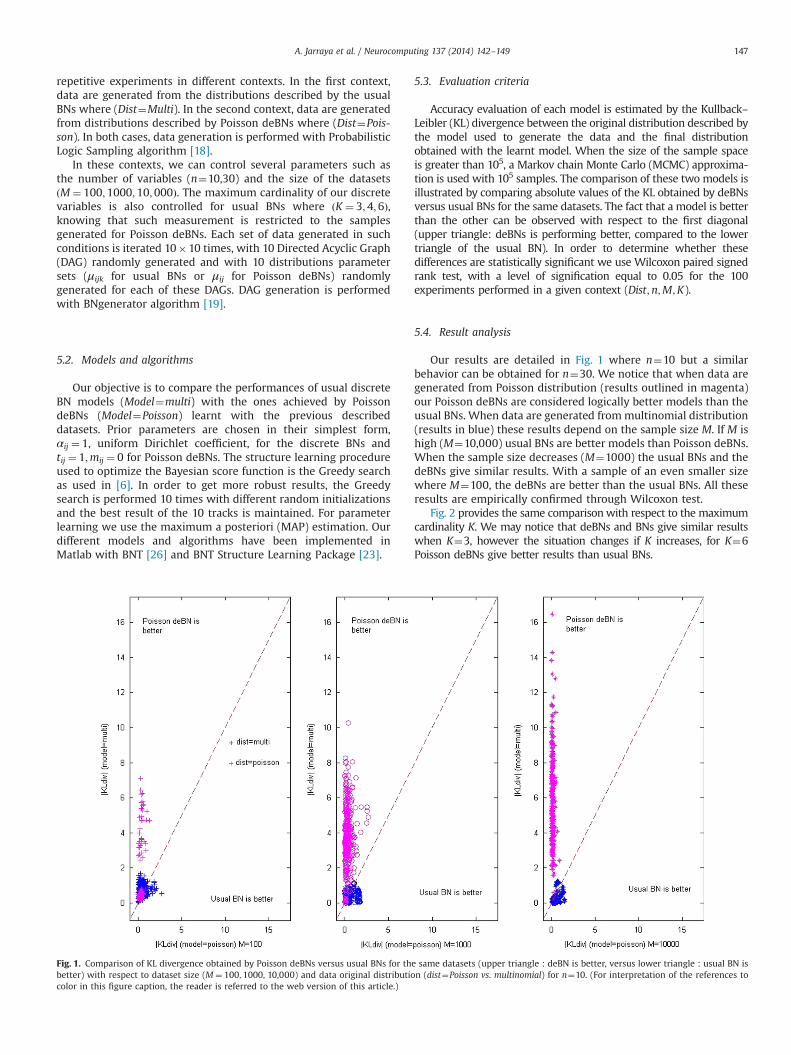
Accuracy evaluation of each model is estimated by the Kullback–Leibler (KL) divergence between the original distribution described bythe model used to generate the data and the final distributionobtained with the learnt model. When the size of the sample spaceis greater than 105, a Markov chain Monte Carlo (MCMC) approxima-tion is used with 105 samples. The comparison of these two models isillustrated by comparing absolute values of the KL obtained by deBNsversus usual BNs for the same datasets. The fact that a model is betterthan the other can be observed with respect to the first diagonal(upper triangle: deBNs is performing better, compared to the lowertriangle of the usual BN). In order to determine whether thesedifferences are statistically significant we use Wilcoxon paired signedrank test, with a level of signification equal to 0.05 for the 100experiments performed in a given context (Dist;n;M;K).

5.4. Result analysis

Our results are detailed in Fig. 1 where n¼10 but a similarbehavior can be obtained for n¼30. We notice that when data aregenerated from Poisson distribution (results outlined in magenta)our Poisson deBNs are considered logically better models than theusual BNs. When data are generated frommultinomial distribution(results in blue) these results depend on the sample size M. If M ishigh (M¼10,000) usual BNs are better models than Poisson deBNs.When the sample size decreases (M¼1000) the usual BNs and thedeBNs give similar results. With a sample of an even smaller sizewhere M¼100, the deBNs are better than the usual BNs. All theseresults are empirically confirmed through Wilcoxon test.

Fig. 2 provides the same comparisonwith respect to the maximumcardinality K. We may notice that deBNs and BNs give similar resultswhen K¼3, however the situation changes if K increases, for K¼6Poisson deBNs give better results than usual BNs.

Fig. 1. Comparison of KL divergence obtained by Poisson deBNs versus usual BNs for the same datasets (upper triangle : deBN is better, versus lower triangle : usual BN isbetter) with respect to dataset size (M ¼ 100;1000, 10,000) and data original distribution (dist¼Poisson vs. multinomial) for n¼10. (For interpretation of the references tocolor in this figure caption, the reader is referred to the web version of this article.)

A. Jarraya et al. / Neurocomputing 137 (2014) 142–149 147

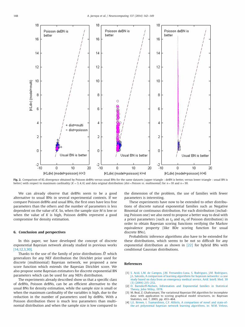
We can already observe that deBNs seem to be a goodalternative to usual BNs in several experimental contexts. If wecompare Poisson deBNs and usual BNs, the first ones have less freeparameters than the others and the number of parameters is lessdependent on the value of K. So, when the sample size M is low orwhen the value of K is high, Poisson deBNs represent a goodcompromise for density estimation.

6. Conclusion and perspectives

In this paper, we have developed the concept of discreteexponential Bayesian network already studied in previous works[14,12,3,30].

Thanks to the use of the family of prior distributions ~Π whichgeneralizes for any NEF distribution the Dirichlet prior used fordiscrete (multinomial) Bayesian network, we proposed a newscore function which extends the Bayesian Dirichlet score. Wealso propose some Bayesian estimators for discrete exponential BNparameters which can be used for any NEFs distribution.

The experiments already described show us that a specific classof deBNs, Poisson deBNs, can be an efficient alternative to theusual BNs for density estimation, while the sample size is small orwhen the maximum cardinality of the variables is high, due to thereduction in the number of parameters used by deBNs. With aPoisson distribution there is much less parameters than multi-nomial distribution and when the sample size is low compared to

the dimension of the problem, the use of families with fewerparameters is interesting.

These experiments have now to be extended to other distribu-tions of discrete natural exponential families such as NegativeBinomial or continuous distribution. For each distribution (includ-ing Poisson one) we also need to propose a better way to deal witha priori parameters (such as tij and mij of Poisson distribution) inorder to obtain Bayesian scoring functions verifying the Markovequivalence property (like BDe scoring function for usualdiscrete BNs).

Probabilistic inference algorithms also have to be extended forthese distributions, which seems to be not so difficult for anyexponential distribution as shown in [22] for hybrid BNs withconditional Gaussian distributions.

References

[1] S. Acid, L.M. de Campos, J.M. Fernandez-Luna, S. Rodriguez, J.M. Rodriguez,J.L. Salcedo, A comparison of learning algorithms for bayesian networks: a casestudy based on data from an emergency medical service, Artif. Intell. Med. 30(3) (2004) 215–232.

[2] O. Barndorff-Nielsen, Information and Exponential families in StatisticalTheory, John Wiley, 1978.

[3] M. Beal, Z. Ghahramani, The variational Bayesian EM algorithm for incompletedata: with application to scoring graphical model structures, in: BayesianStatistics, vol. 7, 2003, pp. 453–464.

[4] L.E. Brown, I. Tsamardinos, C.F. Aliferis, A comparison of novel and state-of-the-art polynomial bayesian network learning algorithms, in: M.M. Veloso,

Fig. 2. Comparison of KL divergence obtained by Poisson deBNs versus usual BNs for the same datasets (upper triangle : deBN is better, versus lower triangle : usual BN isbetter) with respect to maximum cardinality (K ¼ 3;4;6) and data original distribution (dist¼Poisson vs. multinomial) for n¼10 and n¼30.

A. Jarraya et al. / Neurocomputing 137 (2014) 142–149148

S. Kambhampati (Eds.), Proceedings of the Twentieth National Conference onArtificial Intelligence, AAAI Press, 2005, pp. 739–745.

[5] D. Chickering, D. Geiger, D. Heckerman, Learning Bayesian Networks is NP-Hard, Technical Report MSR-TR-94-17, Microsoft Research Technical Report,1994.

[6] D. Chickering, D. Geiger, D. Heckerman, Learning Bayesian networks: searchmethods and experimental results, in: Proceedings of Fifth Conference onArtificial Intelligence and Statistics, 1995, pp. 112–128.

[7] D. Chickering, D. Heckerman, Efficient approximation for the marginal like-lihood of incomplete data given a Bayesian network, in: UAI'96, MorganKaufmann, 1996, pp. 158–168.

[8] G. Consonni, P. Veronese, Conjugate priors for exponential families havingquadratic variance functions, J. Am. Stat. Assoc. 87 (1992) 1123–1127.

[9] R. Daly, Q. Shen, S. Aitken, Learning bayesian networks: approaches and issues,Knowl. Eng. Rev. 26 (2011) 99–157.

[10] P. Diaconis, D. Ylvisaker, Conjugate priors for exponential families, Ann. Stat. 7(1979) 269–281.

[11] L.D. Fu, 2005, A Comparison of State-of-the-Art Algorithms for LearningBayesian Network Structure from Continuous Data, Master's Thesis, VanderbiltUniversity.

[12] D. Geiger, D. Heckerman, H. King, C. Meek, Stratified exponential families:graphical models and model selection, Ann. Stat 29 (2001) 505–529.

[13] D. Geiger, D. Heckerman, C. Meek, Asymptotic model selection for directednetworks with hidden variables, in: Proceedings of the Twelfth AnnualConference on Uncertainty in Artificial Intelligence (UAI–96), Morgan Kauf-mann Publishers, San Francisco, CA, 1996, pp. 283–290.

[14] D. Geiger, C. Meek, Graphical models and exponential families, in: Proceedingsof Fourteenth Conference on Uncertainty in Artificial Intelligence, Madison,WI, Morgan Kaufmann, 1998, pp. 156–165.

[15] A. Hassairi, La classification des familles exponentielles naturelles sur Rn parl'action du groupe linéaire de Rnþ1, C.R. Acad. Sci. Paris Sér. I Math. 315 (1992)207–210.

[16] D. Heckerman, A tutorial on learning with Bayesian networks, in: M.I. Jordan(Ed.), Learning in Graphical Models, Kluwer Academic Publishers, Boston,1998, pp. 301–354.

[17] D. Heckerman, D. Geiger, D. Chickering, Learning Bayesian networks: thecombination of knowledge and statistical data, Mach. Learn. 20 (1995)197–243.

[18] M. Henrion, Propagating uncertainty in Bayesian networks by probabilisticlogic sampling, in: Uncertainty in Artificial Intelligence Second Annual Con-ference on Uncertainty in Artificial Intelligence (UAI-86), Elsevier Science,Amsterdam, NL, 1986, pp. 149–163.

[19] J. Ide, F. Cozman, F. Ramos, Generating random Bayesian networks withconstraints on induced width, in: Proceedings of the European Conferenceon Artificial Intelligence (ECAI 2004), 2004, pp. 323–327.

[20] A. Jarraya, P. Leray, A. Masmoudi, Discrete exponential Bayesian networks: anextension of Bayesian networks to discrete natural exponential families, in:23rd IEEE International Conference on Tools with Artificial Intelligence(ICTAI'2011), Boca Raton, Florida, USA, 2011, pp. 205–208.

[21] A. Jarraya, P. Leray, A. Masmoudi, Discrete exponential Bayesian networksstructure learning for density estimation, in: Proceedings of the 2012 EighthInternational Conference on Intelligent Computing (ICIC 2012), Springer,Huangshan, China, 2012, pp. 146–151.

[22] S.L. Lauritzen, F. Jensen, Stable local computation with conditional Gaussiandistributions, Stat. Comput. 11 (2001) 191–203.

[23] P. Leray, O. Francois, BNT Structure Learning Package: Documentation andExperiments, Technical Report, Laboratoire PSI, 2004.

[24] G. Letac, Lectures on Natural Exponential Families and their Variance Func-tions, Number 50 in Monograph. Math., Inst. Mat. Pura Aplic. Rio., 1992.

[25] C.N. Morris, Natural exponential families with quadratic variance functions,Ann. Stat. 10 (1982) 65–80.

[26] K. Murphy, The Bayes Net Toolbox for Matlab, Comput. Sci. Stat. 33 (2001)1024–1034.

[27] H. Raiffa, R. Schlaifer, Applied Statistical Decision Theory, Graduate School ofBusiness Administration, Harvard University, Boston, 1961.

[28] M. Studený, Mathematical Aspects of Learning Bayesian Networks: BayesianQuality Criteria, Research Report 2234, Institute of Information Theory andAutomation, Prague, 2008.

[29] I. Tsamardinos, L. Brown, C. Aliferis, The max-min hill-climbing Bayesiannetwork structure learning algorithm, Mach. Learn. 65 (1) (2006) 31–78.

[30] M.J. Wainwright, M.I. Jordan, Graphical models, exponential families, andvariational inference, Found. Trends Mach. Learn. 1 (2008) 1–305.

Aida Jarraya got her Bachelor in 2003 and received aMaster degree on Applied Mathematics in Faculty ofSciences of Sfax, Tunisia. she is a very active member ofthe research unit “Probability and Statistics”. She is adoctoral student registered in the third year Ph.D.student jointly supervised. This thesis is part of acommon research theme to Knowledge and DecisionTeam, University of Nantes, and the Laboratory ofProbability and Statistics, University of Sfax. The workof her thesis is at the intersection between appliedmathematics and computer science, and designed spe-cifically for the application of recent theoreticaladvances in statistics in the context of Bayesian

Networks. She is also contractual assistant in the University of Sfax for 3 years(2009–2012).

Philippe Leray graduated from a French engineeringschool in Computer Sciences in 1993. He also got a Ph.D. (Computer Sciences) from the University Paris 6 in1998, about the use of bayesian and neural networksfor complex system diagnosis. Since 2007, he is a fullprofessor at Polytech'Nantes, a pluridisciplinary FrenchEngineering University, teaching from basic statistics toprobabilistic graphical models. He has been workingmore intensively on Bayesian Networks field for thepast 12 years with interests for theory (Bayesian net-work structure learning, causality) and application(reliability, intrusion detection, bio-informatics). SinceJanuary 2012, he is also the head of the “Knowledge

and Decision” research group, in the Nantes Computer Science lab. This researchgroup is structured around three main research themes, Data mining (associationrule mining and clustering) and Machine learning (probabilistic graphical models),Knowledge engineering, and Knowledge visualization, with a Transverse ambition,improving the performance, in terms of complexity but also “actionability” ofmining and learning algorithms by integrating domain and/or user knowledge.

Afif Masmoudi graduated from Sfax University. He alsogot a Ph.D. (Mathematics) from the University of Sfax in2000, about the asymptotic properties of a variancefunction on the means boundary. Since 2010, he is a fullprofessor at Faculty of Science of Sfax, teaching from basicstatistics and probability. He has been working moreintensively on exponential families and Bayesian estima-tion and application. He is a member of Laboratory ofStatistics and Probability of Sfax. The interest research isaround: Statistical inference; Statistical modelling; Expo-nential families; Distribution theory; Estimating functions;Stochastic processes; Generalized linear mixed models,probabilistic graphical models, and Bayesian Network.

A. Jarraya et al. / Neurocomputing 137 (2014) 142–149 149