Discrete Element Method Lagggrangian approach used in ...

Discrete Element Method (DEM) simulations: A(DEM) simulations: A Lagrangian approach used g g ppin granular materials and multiphase flowsmultiphase flows

Payman JalaliAdjunct [email protected]

ContentsContents

• Granular Materials, Gas-Solid Systems and Lagrangian Models

• Discrete Element Method (DEM) ( )

• Applications in Dense Packs

• Applications in Dilute Systems: Comparison to Eulerian Models

• Linking 1D Gas Flow to DEM• Linking 1D Gas Flow to DEM

• Other Lagrangian Methods: Hard Sphere (Disk) Model

Granular Materials, Gas-SolidSystems and Lagrangian Models

• Granular material, a collection of solid grains as a bulk

• It behaves strangely: A fourth state of matter (continuum media?)g y f ( )

• Deformation (or its rate) not uniform

Eff f i i i l fl id• Effects of interstitial fluid

• Size and shape of individual grains

• Mechanical properties of individual grains


Gas Solid systems are mainly found inGas-Solid systems are mainly found influidized beds with different processesinvolved such as combustion, gasification,drying or simply heat transferdrying, or simply heat transfer.


Why Lagrangian models are needed?

• Complex dynamics of granular phase can be explained and• Complex dynamics of granular phase can be explained and

understood by modeling in particle scale.

• The results can be extended to verify/modify the Eulerian models

used in very large industrial systemsused in very large industrial systems.

• Sometimes they are the only way to study particulate systems

such as the study of large particle packing.

Discrete Element Method (DEM)Discrete Element Method (DEM)

Scale based classification of simulations

Micro‐Scale Meso‐Scale Macro‐Scale

Scale-based classification of simulations

Micro Scale

Individual particle base

Meso Scale

Local cell base

Macro Scale

System base

DEMParticleMotion

Trajectories of individual particles

Continuummodel(multi‐dimension)

Continuum model(one‐dimension)

FluidMotion

Flow aroundindividual particles

Local averaging(multi‐dimension)

One‐dimensional

Two fluidDNS

L‐EL‐E

DNS: Direct Numerical Simulation

Two‐fluidmodel (E‐E)

DNS

E: Eulerian

L: Lagrangian


i Fi

CnijF

CtijF

j

nij

jijn

jtij

Forces from Hertzian theory:

KF )( 2/3

sijtjtijtCtij

ijijrijnjnijnCnij

k

K

vδF

nnvF

)( 2/3

ijjiiijijrijrijsij

jirij

nωωrnnvvv

vvv

)()(

tCtijtij

ijCnijfCtijCnijfCtij kFδ

tFFFF

/ If

jCtijCnijCi )( FFF

sijsijij

tCtijtij

vvt /

j

CtijijsiCi

j

r )( FnT

Discrete Element Method (DEM)

Th l iff K i l iff


The normal stiffness Kn, tangential stiffnesskt, and damping factors n and t areobtained from the Hertzian theory:

214 RRK

212

22

1

21 113 RR

EE

Kn

2/1

21

21

228

nijt

RR

RRk

2121

RRGG

modulus sYoung' :E :modulusShear E

Radius :ratio sPoisson' :

R

)1(2

EG


The damping factor can be determined by:

Here, varies between 0 and 1 mostly and it is related to the coefficient of i i

4/12/1)( nijntn mK

restitution.

22 )(ln)ln(5

ee


START


START

Read Initial datadata

Build the table for potential contacting

Contact forces on each particle & potential contacting

neighborsp

deformations

Yes

Torques on each particleIf t<tf ?STOP

No

Linear & angular accelerations using forces &

Velocities & positions at new ti t

Update neighbors list if needed using forces &

torquestime steplist if needed

Applications in Dense PacksApplications in Dense Packs

Vibration of granular beds

Applications in Dense PacksApplications in Dense Packs

Stacking and sedimentation of particlesApplication in nuclear pebble bed reactor(H. Suikkanen, J. Ritvanen, P. Jalali)

• 400 000 fuel particles are settled under gravity.• The environment of each particle is analyzed byV i llVoronoi cells.• The overall packing properties studied.• The DEM code is parallel.• Real earthquake signal is applied to see the• Real earthquake signal is applied to see thechanges caused by it.

Applications in Dilute Systems: Comparison to Eulerian ModelsIn a typical fluidized bed system there are several phases involved The gas (or liquid)In a typical fluidized bed system, there are several phases involved. The gas (or liquid)phase is the background phase and the solid phases are the dispersed phases. InEulerian approach (multi-fluid model), the above-mentioned system is considered as amixture of 3 continuamixture of 3 continua.

Gas phase

Solid phase 1

Gas phase

Solid phase 1

Solid phase 2

Solid phase 1

Solid phase 2

+ +1s

Gas flow

g2s

Applications in Dilute Systems: Comparison to Eulerian Models

G i tiGoverning equations• Conservation of mass for phase k:

kkkt

)()( u

Mass transfer to phase k from other phases

tk phase offraction volume:k

0,111

n

kk

n

kk

11 kk

• Conservation of momentum for phase k:

gFuuu kkkkkkk p )()()(

Transient term Convectiveterm

Stress withinphase k

Momentumtransfer between

gkkkkkkk pt

)()()(

term phase k phases


S f th f b t h li t d b l D di th t t f h

MTWMDTDVMLpD FFFFFFFFF

• Some of the forces between phases are listed below. Depending on the state of phases

(gas, solid or liquid) the significance of each term varies.MTk

Wk

MDk

TDk

VMk

Lk

pk

Dkk FFFFFFFFF

- D: drag force

p: interfacial pressure force

- TD: turbulent diffusion force

- MD: mass diffusion force- p: interfacial pressure force

- L: lift force

- VM: virtual mass force

MD: mass diffusion force

- W: wall repulsion force

- MT: force due to mass transfer betweenphasesphases

Applications in Dilute Systems: Comparison to Eulerian ModelsWe investigated the solid-solid phases interaction using DEM:We investigated the solid solid phases interaction using DEM:

Red and black dots represent the particles of each phase. Initially, blackparticles are fixed and red ones move. Due to collisional drag, the momentumi t f d t th bl k his transferred to the black phase.

The overall view of the mixture

View of a control volumeinside the system

Applications in Dilute Systems:

The momentum transfer between the solid phases (F ) per unit volume can be also

Comparison to Eulerian ModelsThe momentum transfer between the solid phases (Fml) per unit volume can be alsocompared between the DEM model, and the theoretical prediction using data provided bythe DEM (Syamlal/DEM) and the multifluid Eulerian-Eulerian model (Syamlal/FLUENT).

Initial uniform random mixture

)(2)()8/2/)(1(3

)(

330

22

llmm

mllmlmlmml

mlmlml

ddgdde

I

I

vv

vvF

Syamlal/FLUENT

DEM

Syamlal/DEMy


M d il b f d i f ll i bli iMore details can be found in our following publication:


The collisional drag from a particle cloud on large particles is important in systems such asThe collisional drag from a particle cloud on large particles is important in systems such asbiomass. DEM simulations are used along with Eulerian simulations to study these forces.

Linking 1D Gas Flow to DEMLinking 1D Gas Flow to DEM

• Continuity:

011

iigi

ig uu

y

p

• Momentum:

11

1

1

1 )(1i

iii

ig

ii vxAppA

uu

Continuity cellMomentum cell

pi

pi+1Ai+1,ui+1

111

1 )( ig

iig

ii

i Mpp

ME

Ai,ui

80)1(3

8.0,)1(75.1)1(150

7.2

2

2

ii

igsp

gig

pi

i

i

vvC

vvdd

8.0,4 iigsg

pD vv

dC

1000R4301000ReRe,/)Re15.01(24 687.0

DC

1000Re,43.0D

Particle Reynolds number


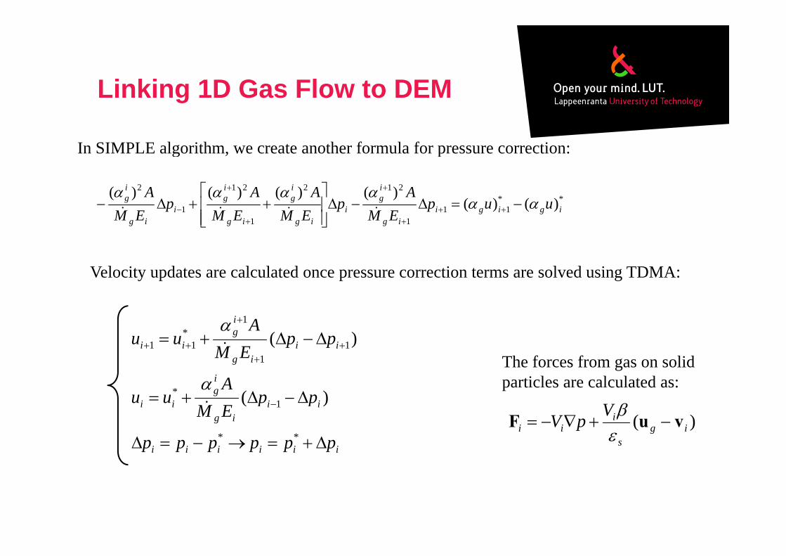
In SIMPLE algorithm, we create another formula for pressure correction:

**11

21221

1

2

)()()()()()(

igigi

ig

i

ig

ig

i

ig uup

EMA

pEM

AEM

Ap

EMA

In SIMPLE algorithm, we create another formula for pressure correction:

11 igigigig EMEMEMEM

Velocity updates are calculated once pressure correction terms are solved using TDMA:y p p g

ig pp

Auu

1* )(

ii

ig

ii

iiig

ii

ppA

uu

ppEM

uu

1*

11

11

)(

)(

The forces from gas on solidparticles are calculated as:

V

iiiiii

iiig

ii

pppppp

ppEM

**

1 )()( ig

s

iii

VpV vuF


0.145m x 0.01mPo=110000 Pa

0.270GPaE1000N

mm5

d p

3m

40.0kg/m2500

0.33

e

kg/m205.1

kg/s025.03

gM

Pa.s1011.15 6

Other Lagrangian Methods: HardSphere (Disk) Model

V11ωAn event-driven algorithm:

• Dynamics of system is only governed by particle-particleinteractions.

V1

V2

• Particles are hard disks and they interact via binarycollisions. 2ω

k

• Collision times are calculated numerically as gravity and a constrained motion of the obstacle particles may exist.


V’' V 11ω'

V’

V11ω

V 2

2'ω

V2

k

Pre collisional status

2

Post collisional status

2ω

Pre-collisional status Post-collisional status

pVVpVV 22'211

'1

dd

Post-collisional

ΓωωΓωω2

22

'2

1

11

'1 22 I

dI

dvelocities

)()( UU)()()()(

12221212222

12211112211

nUnUpnUnUp


e0=0.90 H0

Vy0

N, dP gL

DCylindricalobstacle

D

yx

Thank you for your attention!

Discrete Element Method Lagggrangian approach used in ...

Documents

Transcript of Discrete Element Method Lagggrangian approach used in ...