Discrete and continuous adjoint method for compressible...
61
Discrete and continuous adjoint method for compressible CFD J. Peter ONERA J. Peter 1 1 ONERA DMFN October 2, 2014 J. Peter (ONERA DMFN) Adjoint method for compressible CFD October 2, 2014 1 / 60
Transcript of Discrete and continuous adjoint method for compressible...

Discrete and continuous adjoint method for compressible CFDJ. Peter ONERA
J. Peter1
1ONERA DMFN
October 2, 2014
J. Peter (ONERA DMFN) Adjoint method for compressible CFD October 2, 2014 1 / 60

Introduction
Outline
1 Introduction
2 Discrete adjoint method
3 Continuous adjoint method
4 Discrete vs Continuous adjoint
5 Conclusions
J. Peter (ONERA DMFN) Adjoint method for compressible CFD October 2, 2014 2 / 60

Introduction
Introduction (1/4)
Well-known aerodynamic optimization problems of the utmost importance
Aircraft drag reductionReduction of total pressure losses of a blade row.
Strongly constrained problems (from aerodynamics, structure...)
Several approaches for researches and studies in external aerodynamics
Flight testsWind tunnel experiments (with flight Re/lower than flight Re)Numerical simulation
Numerical simulation most adapted
J. Peter (ONERA DMFN) Adjoint method for compressible CFD October 2, 2014 3 / 60

Introduction
Introduction (2/4)
(Non solvable) pde → numerical simulation. Finite-volume simulation in thistalk.
Infinite dimension possible deformation → parametrization
Finite dimensional maths
Which type of optimization method ?
Local or global optimization ?
J. Peter (ONERA DMFN) Adjoint method for compressible CFD October 2, 2014 4 / 60

Introduction
Introduction (3/4)
Global optimization
genetic/evolutionnary algorithms, particle swarm, aunt colony, CMA-ES...large number of function evaluations requiredcombined with surrogate modelsin particular used for design space exploration with low fidelity models
Local optimization
very valuable when starting from pre-optimized shapespattern methods. e.g. simplex methodgradient-based methods. e.g. steepest descent, conjugate gradient
Popular and efficient descent methods require objective and constraintsensitivities w.r.t. design parameters
J. Peter (ONERA DMFN) Adjoint method for compressible CFD October 2, 2014 5 / 60
Introduction
Introduction (4/4)
Needed sensitivities w.r.t. design parameters
...not a trivial task in numerical simulation as state variables change withshape via the equations of the mechanical problem
Sensitivty calculation
70’s 80’s finite differences. Scaling with number of shape parametersControl theory [Lions 71, Pironneau 73,74] aerodynamics shape optimization[Jameson 88] adjoint method. Scaling with the number of functions to bedifferentiated
Other applications of adjoint method: understanding zones of influence forfunction value, goal-oriented mesh refinement
J. Peter (ONERA DMFN) Adjoint method for compressible CFD October 2, 2014 6 / 60

Discrete adjoint method
Outline
1 Introduction
2 Discrete adjoint method
3 Continuous adjoint method
4 Discrete vs Continuous adjoint
5 Conclusions
J. Peter (ONERA DMFN) Adjoint method for compressible CFD October 2, 2014 7 / 60

Discrete adjoint method
Discrete adjoint method
Framework: compressible flow simulation using finite volume method.Discrete approach for sensitivity analysis
Notations
Volume mesh X , flowfield W (size na)Wall surface mesh SResidual R, C 1 regular w.r.t. X and W – steady state: R(W ,X ) = 0Vector of design parameters α (size nd), X (α) S(α) C 1 regular
Assumption of implicit function theorem
∀ (Wi ,Xi ) / R(Wi ,Xi ) = 0 (∂R/∂W )(Wi ,Xi ) 6= 0Unique steady flow corresponding to a mesh
J. Peter (ONERA DMFN) Adjoint method for compressible CFD October 2, 2014 8 / 60

Discrete adjoint method
IntroductionDiscrete gradient calculation methods
Functions of interest
Jk(α) = Jk(W (α),X (α)) k ∈ [1, nf ]Flowfield and volume mesh linked by flow equations R(W (α),X (α)) = 0
Sensitivities dJk/dαi k ∈ [1, nf ] i ∈ [1, nd ] to be computed
Discrete gradient computation methods
Finite differences – 2nd flow computations (non linear problems, size na)Direct differentiation method – nd linear systems (size na)Adjoint vector method – nf linear systems (size na)
J. Peter (ONERA DMFN) Adjoint method for compressible CFD October 2, 2014 9 / 60

Discrete adjoint method
Finite difference method
Choose steps δαi . Get shifted meshes X (α + δαi ), X (α− δαi )
Solve flows
R(W (α + δαi ),X (α + δαi )) = 0 R(W (α− δαi ),X (α− δαi )) = 0
dW
dαi (FD)
=W (α + δαi )−W (α− δαi )
2δαi
Compute outputs sensitivities
dJkdαi (FD)
=Jk(W (α + δαi ),X (α + δαi ))− Jk(W (α− δαi ),X (α + δαi ))
2δαi
Two issues: definition of δαi , cost of shifted flow solves
J. Peter (ONERA DMFN) Adjoint method for compressible CFD October 2, 2014 10 / 60

Discrete adjoint method
Direct differentiation method (1/2)
Discrete equations for mechanics (set of na non-linear equations )
R(W (α),X (α)) = 0
Differentiation with respect to αi i ∈ [1, nd ]. Derivation of nd linear systemof size na
∂R
∂W
dW
dαi= −(
∂R
∂X
dX
dαi)
Calculation of derivatives
dJkdαi
=∂Jk∂X
dX
dαi+∂Jk∂W
dW
dαi
J. Peter (ONERA DMFN) Adjoint method for compressible CFD October 2, 2014 11 / 60

Discrete adjoint method
Direct differentiation method (2/2)
Gradient vectors
∇αJk(α) =∂Jk∂X
dX
dα+∂Jk∂W
dW
dα
Check the flow sensitivities using finite differences
R(W (α + δαi ),X (α + δαi )) = 0 R(W (α− δαi ),X (α− δαi )) = 0
dW
dαi? ' W (α + δαi )−W (α− δαi )
2δαi
Check the outputs sensitivities
dJkdαi
? ' Jk(W (α + δαi ),X (α + δαi ))− Jk(W (α− δαi ),X (α + δαi ))
2δαi
J. Peter (ONERA DMFN) Adjoint method for compressible CFD October 2, 2014 12 / 60

Discrete adjoint method
Mathematical game (1/4)
Mathematical game in Rn to understand adjoint method
given (f , bi ) ∈ Rn (i ∈ 1, nd), given A ∈M(Rn)
Calculate the values of xi .f A xi = bi i ∈ 1, nd
Solution solving one linear system instead of nd linear systems ???
J. Peter (ONERA DMFN) Adjoint method for compressible CFD October 2, 2014 13 / 60

Discrete adjoint method
Mathematical game (2/4)
Linear algebra reminder: the inverse of the transpose is the transpose of theinverse
MT (M−1)T = (M−1M)T = IT = I
(M−1)TMT = (MM−1)T = IT = I
The notation M−T is suitable for (MT )−1 / (M−1)T
J. Peter (ONERA DMFN) Adjoint method for compressible CFD October 2, 2014 14 / 60

Discrete adjoint method
Mathematical game (3/4)
Mathematical game in Rn to understand adjoint method
given (f , bi ) ∈ Rn (i ∈ 1, nd), given A ∈M(Rn)
Calculate the values of f .xi A xi = bi i ∈ 1, nd
f .xi = f .(A−1bi ) = ((A−1)T f ).bi = (A−T f ).bi efficient solution
Solve AT λ = f Calculate λ.bi i ∈ 1, nd
J. Peter (ONERA DMFN) Adjoint method for compressible CFD October 2, 2014 15 / 60

Discrete adjoint method
Mathematical game (4/4)
Mathematical game in Rn to understand adjoint method
given (fj , bi ) ∈ Rn (i ∈ 1, nd j ∈ 1, nf ), given A ∈M(Rn)
Calculate the values of xi .fj A xi = bi i ∈ 1, nd
Solution solving nd linear systems
Solution solving nf linear systems
J. Peter (ONERA DMFN) Adjoint method for compressible CFD October 2, 2014 16 / 60

Discrete adjoint method
Discrete adjoint parameter method (1/5)
Several ways of deriving the equations of discrete adjoint method. Thefollowing also helps understanding continuous adjoint
Following equalities hold ∀λk ∈ Rna
λTk∂R
∂W
dW
dαi+ λTk (
∂R
∂X
dX
dαi) = 0
dJk(α)
dαi=∂Jk∂X
dX
dαi+∂Jk∂W
dW
dαi+ λTk
∂R
∂W
dW
dαi+ λTk (
∂R
∂X
dX
dαi)
dJk(α)
dαi= (
∂Jk∂W
+ λTk∂R
∂W)dW
dαi+∂Jk∂X
dX
dαi+ λTk (
∂R
∂X
dX
dαi)
J. Peter (ONERA DMFN) Adjoint method for compressible CFD October 2, 2014 17 / 60

Discrete adjoint method
Discrete adjoint parameter method (2/5)
Vector λk defined in order to cancel the factor of the flow sensitivity dWdαi
...
the adjoint equation. λk actually appears to be linked to functions Jk
∂Jk∂W
+ λTk∂R
∂W= 0
Calculation of derivatives
∀i ∈ [1, nd ]dJk(α)
dαi=∂Jk∂X
dX
dαi+ λTk (
∂R
∂X
dX
dαi)
∇αJk(α) =∂Jk∂X
dX
dα+ λTk (
∂R
∂X
dX
dα)
Method with nf and not nd linear systems to solve
J. Peter (ONERA DMFN) Adjoint method for compressible CFD October 2, 2014 18 / 60

Discrete adjoint method
Discrete adjoint parameter method (3/5)
Other ways to derive the discrete adjoint equation
Introduce a LagrangianManipulate direct differentiation gradient expression (like in the mathematicalgame)
From direct method gradient expression
∇αJk(α) =∂Jk∂X
dX
dα+∂Jk∂W
dW
dα
∇αJk(α) =∂Jk∂X
dX
dα− ∂Jk∂W
(dR
dW
)−1dR
dX
dX
dα
∇αJk(α) =∂Jk∂X
dX
dα−
(∂Jk∂W
(dR
dW
)−1)
dR
dX
dX
dα
Define λk column vector
J. Peter (ONERA DMFN) Adjoint method for compressible CFD October 2, 2014 19 / 60
Discrete adjoint method
Discrete adjoint parameter method (4/5)
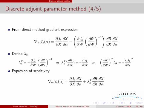
From direct method gradient expression
∇αJk(α) =∂Jk∂X
dX
dα−
(∂Jk∂W
(dR
dW
)−1)
dR
dX
dX
dα
Define λk
λTk = −∂Jk
∂W
(dR
dW
)−1
or λTk (dR
dW) = −
∂Jk
∂Wor
(dR
dW
)T
λk = −∂Jk
∂W
T
Expresion of sensitivity
∇αJk(α) =∂Jk∂X
dX
dα+ λTk
dR
dX
dX
dα
J. Peter (ONERA DMFN) Adjoint method for compressible CFD October 2, 2014 20 / 60

Discrete adjoint method
Iterative solution of direct and adjoint equation (1/3)
CFD teams tend to mimic the solution of steady state flow altough flowequations are non-linear whereas direct/adjoint equation are linear
Storing the jacobian of the scheme and sending to direct solver has beendone but is rare and is not tractable for large cases
Iterative resolution is much more common. Newton/relaxation algorithm(∂R
∂W
)(APP) T (λ
(l+1)k − λ(l)
k
)= −
((∂R
∂W)Tλ
(l)k + (
∂Jk∂W
)T)
J. Peter (ONERA DMFN) Adjoint method for compressible CFD October 2, 2014 21 / 60
Discrete adjoint method
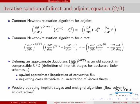
Iterative solution of direct and adjoint equation (2/3)
Common Newton/relaxation algorithm for adjoint(∂R
∂W
)(APP) T (λ
(l+1)k − λ(l)
k
)= −
((∂R
∂W)Tλ
(l)k +
∂Jk
∂W)T)
Common Newton/relaxation algorithm for direct(∂R
∂W
)(APP) ((dW
dαi)(l+1) − (
dW
dαi)(l)
)= −
((∂R
∂W)dW
dαi
(l)
+∂R
∂X
dX
dαi
)
Defining an approximate Jacobians ( ∂R∂W )(APP) is an old subject incompressible CFD (definition of implicit stages for backward-Eulerschemes...)
upwind approximate linearization of convective fluxneglecting cross derivatives in linearization of viscous fluxes...
Possibly adapting implicit stages and mutigrid algorithm (flow solver toadjoint solver)
J. Peter (ONERA DMFN) Adjoint method for compressible CFD October 2, 2014 22 / 60

Discrete adjoint method
Iterative solution of direct and adjoint equation (3/3)
Common Newton/relaxation algorithm for adjoint(∂R
∂W
)(APP) T (λ
(l+1)k − λ(l)
k
)= −
((∂R
∂W)Tλ
(l)k +
∂Jk
∂W)T)
Accuracy of adjoint vector only depends on ( ∂R∂W ). Only minor simplifcationsare allowed at this stage to perserve an acceptable accuracy
Convergence towards solution of the linear system depends on ( ∂R∂W ),
( ∂R∂W )(APP), multigrid (if active), other operations like smoothing (if active)
J. Peter (ONERA DMFN) Adjoint method for compressible CFD October 2, 2014 23 / 60

Discrete adjoint method
Discrete adjoint parameter method (5/5)
Checking adjoint method... much more difficult than checking directdifferentiation method. If
dJkdαi
<>Jk (W (α+ δαi ),X (α+ δαi ))− Jk (W (α− δαi ),X (α+ δαi ))
2δαi
no easy checking procedure
In the iterative resolution method, the gradient accuracy depends on the
( ∂R∂W )Tλ(l)k operation
If direct mode is coded, duality checks between direct and adjoint code areuseful. (U,V ) two column vectors of Rna
UT (∂R
∂W)V =
(UT (
∂R
∂W)
)adj−code
.V = UT .
((∂R
∂W)V
)lin−code
Valid for individual fluxes routine. Valid for part of the interfaces (border,joins...)
J. Peter (ONERA DMFN) Adjoint method for compressible CFD October 2, 2014 24 / 60

Discrete adjoint method
Discrete adjoint mesh method (1/3)
Vector λk defined by∂Jk∂W
+ λTk∂R
∂W= 0
Calculation of derivatives
∀i ∈ [1, nf ]dJk(α)
dαi=∂Jk∂X
dX
dαi+ λTk (
∂R
∂X
dX
dαi)
∀i ∈ [1, nf ]dJk(α)
dαi= (
∂Jk∂X
+ λTk∂R
∂X)dX
dαi
Obvious mathematical factorization. Huge practical importance.
J. Peter (ONERA DMFN) Adjoint method for compressible CFD October 2, 2014 25 / 60
Discrete adjoint method
Discrete adjoint mesh method (2/3)
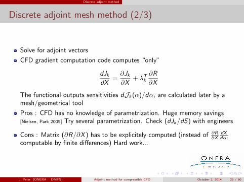
Solve for adjoint vectors
CFD gradient computation code computes “only”
dJkdX
=∂Jk∂X
+ λTk∂R
∂X
The functional outputs sensitivities dJk(α)/dαi are calculated later by amesh/geometrical tool
Pros : CFD has no knowledge of parametrization. Huge memory savings[Nielsen, Park 2005] Try several parametrization. Check (dJk/dS) with engineers
Cons : Matrix (∂R/∂X ) has to be explicitely computed (instead of ∂R∂X
dXdαi
computable by finite differences) Hard work...
J. Peter (ONERA DMFN) Adjoint method for compressible CFD October 2, 2014 26 / 60
Discrete adjoint method
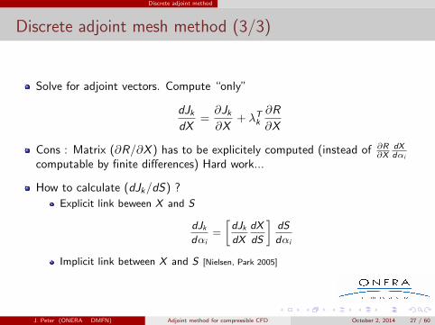
Discrete adjoint mesh method (3/3)
Solve for adjoint vectors. Compute “only”
dJkdX
=∂Jk∂X
+ λTk∂R
∂X
Cons : Matrix (∂R/∂X ) has to be explicitely computed (instead of ∂R∂X
dXdαi
computable by finite differences) Hard work...
How to calculate (dJk/dS) ?
Explicit link beween X and S
dJkdαi
=
[dJkdX
dX
dS
]dS
dαi
Implicit link between X and S [Nielsen, Park 2005]
J. Peter (ONERA DMFN) Adjoint method for compressible CFD October 2, 2014 27 / 60

Continuous adjoint method
Outline
1 Introduction
2 Discrete adjoint method
3 Continuous adjoint method
4 Discrete vs Continuous adjoint
5 Conclusions
J. Peter (ONERA DMFN) Adjoint method for compressible CFD October 2, 2014 28 / 60

Continuous adjoint method
Bibliography
Mathematical references [Pironneau 73,74]
Mathematical aeronautical reference [Jameson 88]
Simplest introduction [Giles, Pierce 99]
An introduction to the adjoint approach to design ERCOFTAC Workshop onAdjoint Methods, Toulouse 1999.
J. Peter (ONERA DMFN) Adjoint method for compressible CFD October 2, 2014 29 / 60

Continuous adjoint method
Continuous Adjoint for toy problems (1/6)
From [Giles, Pierce 99] section (3.2)
Toy problems without design parameters
Solvedu
dx− εd
2u
dx2= f on [0, 1] u(0) = u(1) = 0
before calculating
J = (u, g) =
∫ 1
0
u g dx
Adjoint problem ? Define (if it exists)
L∗λ = g on [0, 1] plus boundary conditions
such that
J = (λ, f ) =
∫ 1
0
λ fdx
J. Peter (ONERA DMFN) Adjoint method for compressible CFD October 2, 2014 30 / 60

Continuous adjoint method
Continuous Adjoint for toy problems (2/6)
Direct: solve
du
dx− εd
2u
dx2= f on [0, 1] u(0) = u(1) = 0
before calculating
J = (u, g) =
∫ 1
0
u gdx
Adjoint problem (if it exists):
L∗λ = g on [0, 1]
plus boundary conditions such that
J = (λ, f ) =
∫ 1
0
λ fdx
Defining equation L∗
J. Peter (ONERA DMFN) Adjoint method for compressible CFD October 2, 2014 31 / 60

Continuous adjoint method
Continuous Adjoint for toy problems (3/6)
Defining equation L∗
(λ, f ) =
∫ 1
0
λ fdx =
∫ 1
0
λ
(du
dx− εd
2u
dx2
)dx
(λ, f ) = −∫ 1
0
dλ
dxu dx + [λ u]1
0 + ε
∫ 1
0
dλ
dx
du
dxdx − ε
[λ
du
dx
]1
0
(λ, f ) = −∫ 1
0
dλ
dxu dx + [λ u]1
0 − ε∫ 1
0
d2λ
dx2du dx − ε
[λdu
dx
]1
0
− ε[dλ
dxu
]1
0
Finally
(λ, f ) =
∫ 1
0
(dλ
dx− εd
2λ
dx2
)udx + [λ u]1
0 + ε
[dλ
dxu
]1
0
− ε[λdu
dx
]1
0
Suitable adjoint equation. Solving
−dλ
dx− εd
2λ
dx2= g on [0, 1] λ(0) = λ(1) = 0
ensures (λ, f ) = (u, g)
J. Peter (ONERA DMFN) Adjoint method for compressible CFD October 2, 2014 32 / 60

Continuous adjoint method
Continuous Adjoint for toy problems (4/6)
In order to calculate J = (u, g) =
∫Ω
u g dΩ, solve for u
div(k grad(u)) = f on Ω u = 0 on ∂Ω
In order to calculate J as (λ, f ) =
∫Ω
λ f dΩ, solve for λ
div(k grad(λ)) = g on Ω λ = 0 on∂Ω
Definition of adjoint operator comes from
(λ, f ) =
∫Ω
u div(k grad(λ))dΩ−∫∂Ω
k u (grad(λ).n)dS +
∫∂Ω
k λ (grad(u).n)dS
J. Peter (ONERA DMFN) Adjoint method for compressible CFD October 2, 2014 33 / 60

Continuous adjoint method
Continuous Adjoint for toy problems (5/6)
Direct: solve
∂u
∂t− ∂2u
∂x2= f on [0, L]× [0,T ] u(0, .) = u(L, .) = 0 u(., 0) = 0
before calculating
J = (u, g) =
∫ L
0
∫ T
0
u g dxdt
Adjoint: solve
−∂λ∂t− ∂2λ
∂x2= g on [0, L]× [0,T ] λ(0, .) = λ(L, .) = 0 λ(.,T ) = 0
before calculating J as
(λ, f ) =
∫ L
0
∫ T
0
λ f dxdt
J. Peter (ONERA DMFN) Adjoint method for compressible CFD October 2, 2014 34 / 60

Continuous adjoint method
Continuous Adjoint for toy problems (6/6)
Time derivative∂u
∂tgets −∂λ
∂tBackward time integration for unsteady adjoint
Convection term∂u
∂xgets −∂λ
∂x“Backward propagation” in adjoint steady state solutions
Diffusion term∂2u
∂x2gets
∂2λ
∂x2
J. Peter (ONERA DMFN) Adjoint method for compressible CFD October 2, 2014 35 / 60

Continuous adjoint method
Continuous Adjoint for 2D Euler equations (1/11)
2D Euler equations∂w
∂t+∂f (w)
∂x+∂g(w)
∂y= 0
avec
w =
ρρuρvρE
f (w) =
ρu
ρu2 + pρuvρHu
g(w) =
ρvρuv
ρv2 + pρHv
p = (γ − 1)ρ(E − u2 + v2
2), ρH = ρE + p
J. Peter (ONERA DMFN) Adjoint method for compressible CFD October 2, 2014 36 / 60

Continuous adjoint method
Continuous Adjoint for 2D Euler equations (2/11)
Figure: Coordinate transformation for airfoil-fitted structured mesh
Coordinate transformation Γ, C 1 diffeomorphism Dξη =[ξmin, ξmax ]× [ηmin, ηmax ] en Dw .
Γ
Dξη → Dxy
(ξ, η) → (x , y)
J. Peter (ONERA DMFN) Adjoint method for compressible CFD October 2, 2014 37 / 60

Continuous adjoint method
Continuous Adjoint for 2D Euler equations (3/11)
Figure: Normal surface vectors
J. Peter (ONERA DMFN) Adjoint method for compressible CFD October 2, 2014 38 / 60

Continuous adjoint method
Continuous Adjoint for 2D Euler equations (4/11)
2D Euler equations generalized coordinates
K = (∂x
∂ξ
∂y
∂η− ∂y
∂ξ
∂x
∂η)
(UV
)=
1
K
∂y∂η
− ∂x∂η
−∂y∂ξ
∂x∂ξ
( uv
)
W = K
ρρuρvρE
F (W ) = K
ρU
ρUu + p ∂ξ∂x
ρUv + p ∂ξ∂y
ρUH
G(W ) = K
ρV
ρVu + p ∂η∂x
ρVv + p ∂η∂y
ρVH
∂W
∂t+∂F (W )
∂ξ+∂G(W )
∂η= 0
J. Peter (ONERA DMFN) Adjoint method for compressible CFD October 2, 2014 39 / 60

Continuous adjoint method
Continuous Adjoint for 2D Euler equations (5/11)
Steady state equation can also be rewritten as
∂
∂ξ
(f∂y
∂η− g
∂x
∂η
)+
∂
∂η
(−f ∂y
∂ξ+ g
∂x
∂ξ
)= 0 sur Dξη
Jacobians per mesh directions :
a(w) =df (w)
dwb(w) =
dg(w)
dw
a1(w , ξ, η) =
(a(w)
∂y
∂η− b(w)
∂x
∂η
)a2(w , ξ, η) =
(−a(w)
∂y
∂ξ+ b(w)
∂x
∂ξ
)
J. Peter (ONERA DMFN) Adjoint method for compressible CFD October 2, 2014 40 / 60

Continuous adjoint method
Continuous Adjoint for 2D Euler equations (6/11)
Coordinate transformation now depending on a design parameter α (for thesake of simplicity scalar)
Γ
DξηDα → Dw
(ξ, η)(α) → (x(ξ, η, α), y(ξ, η, α))(1)
Dw changes with α but not Dξη
Equation for dW /dαi ?
J. Peter (ONERA DMFN) Adjoint method for compressible CFD October 2, 2014 41 / 60

Continuous adjoint method
Continuous Adjoint for 2D Euler equations (7/11)
Variations induced by dα change f (w) → f (w) + dfdw
dwdαi
dαi
∂x∂η
→ ∂x∂η
+ ∂2x∂η∂αi
dαi
Fluid dynamics equations on the fixed domain Dξη
∀ α ∈ Dα∂
∂ξ
(f∂y
∂η− g
∂x
∂η
)+
∂
∂η
(−f ∂y
∂ξ+ g
∂x
∂ξ
)= 0 on Dξη
Differentiate w.r.t. α
J. Peter (ONERA DMFN) Adjoint method for compressible CFD October 2, 2014 42 / 60

Continuous adjoint method
Continuous Adjoint for 2D Euler equations (8/11)
Continuous direct differention equation
∂∂ξ
(a1(w , ξ, η)dwdα
)+ ∂∂η
(a2(w , ξ, η)dwdα
)+
∂∂ξ
(f (w) ∂2y
∂η∂α− g(w) ∂2x
∂η∂α
)+ ∂∂η
(−f (w) ∂
2y∂ξ∂α
+ g(w) ∂2x∂ξ∂α
)= 0
Objective function (fixed domain Dξη)
J (α) =
∫ξmin
J1(w)dη +
∫Dξη
J2(w)dξdη
derivative of the objective function (fixed domain Dξη)
dJ (α)
dα=
∫ξmin
dJ1(w)
dw
dw
dαdη +
∫Dξη
dJ2(w)
dw
dw
dαdξdη
J. Peter (ONERA DMFN) Adjoint method for compressible CFD October 2, 2014 43 / 60

Continuous adjoint method
Continuous Adjoint for 2D Euler equations (9/11)
continuous direct differentiation equation is multiplied by ψ, C 1, periodic inηmin, ηmax
∀ψ ∈ C 1(Dξη)4∫Dξη
ψT(∂∂ξ
(a1(w , ξ, η) dw
dα
)+ ∂∂η
(a2(w , ξ, η) dw
dα
))dξdη+∫
DξηψT
(∂∂ξ
(f (w)
∂2y
∂η∂α− g(w) ∂
2x∂η∂α
)+ ∂∂η
(−f (w)
∂2y
∂ξ∂α+ g(w) ∂
2x∂ξ∂α
))dξdη = 0
Integration by parts
−∫Dξη
∂ψT
∂ξa1(w , ξ, η) dw
dαdξdη −
∫Dξη
∂ψT
∂ηa2(w , ξ, η) dw
dαdξdη+
−∫Dξη
∂ψT
∂ξ
(f (w)
∂2y
∂η∂α− g(w) ∂
2x∂η∂α
)dξdη
−∫Dξη
∂ψT
∂η
(−f (w)
∂2y
∂ξ∂α+ g(w) ∂
2x∂ξ∂α
)dξdη
+∫ξmin
ψT a1(w , ξ, η) dwdα
dη +∫ξmin
ψT
(f (w)
∂2y
∂η∂α− g(w) ∂
2x∂η∂α
)dη = 0.
J. Peter (ONERA DMFN) Adjoint method for compressible CFD October 2, 2014 44 / 60

Continuous adjoint method
Continuous Adjoint for 2D Euler equations (10/11)
Gradient of objective function for all ψ function of C 1η (Dξη)4
dJ (α)dα =
∫ξmin
dJ1(w)dw
dwdα
dη +∫Dξη
dJ2(w)dw
dwdα
dξdη
−∫Dξη
∂ψT
∂ξa1(w , ξ, η) dw
dαdξdη −
∫Dξη
∂ψT
∂ηa2(w , ξ, η) dw
dαdξdη+
−∫Dξη
∂ψT
∂ξ
(f (w)
∂2y
∂η∂α− g(w) ∂
2x∂η∂α
)dξdη
−∫Dξη
∂ψT
∂η
(−f (w)
∂2y
∂ξ∂α+ g(w) ∂
2x∂ξ∂α
)dξdη
+∫ξmin
ψT a1(w , ξ, η) dwdα
dη +∫ξmin
ψT
(f (w)
∂2y
∂η∂α− g(w) ∂
2x∂η∂α
)dη
ψ chosen so as to cancel all flow sensitivity termsdJ2(w)dw
− ∂ψT
∂ξa1(w , ξ, η)− ∂ψ
T
∂ηa2(w , ξ, η) = 0 over Dξ,η
ψT a1(w , ξ, η) +dJ1(w)dw
= 0 on ξmin
J. Peter (ONERA DMFN) Adjoint method for compressible CFD October 2, 2014 45 / 60

Continuous adjoint method
Continuous Adjoint for 2D Euler equations (11/11)
Final form of objective gradient (ψ being the solution of continuous adjointequation)
dJ (α)dαi
=∫ξmin
ψT
(f (w)
∂2y
∂η∂αi− g(w) ∂
2x∂η∂αi
)dη
−∫Dξη
∂ψT
∂ξ
(f (w)
∂2y
∂η∂αi− g(w) ∂
2x∂η∂αi
)dξdη
−∫Dξη
∂ψT
∂η
(−f (w)
∂2y
∂ξ∂αi+ g(w) ∂
2x∂ξ∂αi
)dξdη
(2)
Just as for discrete adjoint, one adjoint field for one function of interest anddesign parameters
Partial differential equation which derivation exceeds level of maths ordinarlyused by engineers
Equation to be discretized to get numerical values
J. Peter (ONERA DMFN) Adjoint method for compressible CFD October 2, 2014 46 / 60

Continuous adjoint method
Some intuitions about adjoint vector ? (1/7)
Could I get some intuition about adjoint vector ?Try again with continuous adjoint !
Rewrite flow equation locally, neglecting metric derivatives terms
∂
∂ξ
(f∂y
∂η− g
∂x
∂η
)+
∂
∂η
(−f ∂y
∂ξ+ g
∂x
∂ξ
)= 0 sur Dξη
a(w) =df (w)
dwb(w) =
dg(w)
dw
a1(w , ξ, η) =
(a(w)
∂y
∂η− b(w)
∂x
∂η
)a2(w , ξ, η) =
(−a(w)
∂y
∂ξ+ b(w)
∂x
∂ξ
)
J. Peter (ONERA DMFN) Adjoint method for compressible CFD October 2, 2014 47 / 60

Continuous adjoint method
Some intuitions about adjoint vector ? (2/7)
Could I get some intuition about adjoint vector ?Trying again based on continuous adjoint
Rewrite flow equation locally, neglecting metric derivatives terms
a1(w , ξ, η)∂w
∂ξ+ a2(w , ξ, η)
∂w
∂η= 0
Reminder adjoint equation
dJ2(w)
dw−∂ψ
T
∂ξa1(w , ξ, η)−
∂ψT
∂ηa2(w , ξ, η) = 0
Change of sign, transposed jacobians, source term.
Hyperbolic system. Same conditions for existence of simple wave solutionsψ(ξ, η) = Ψ(aξ + bη)V , propagation par convection. Number of solutions forsubsonic/supersonic flow...
J. Peter (ONERA DMFN) Adjoint method for compressible CFD October 2, 2014 48 / 60
Continuous adjoint method
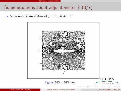
Some intuitions about adjoint vector ? (3/7)
Supersonic inviscid flow M∞ = 1.5 AoA = 1o
Figure: 513 × 513 mesh
J. Peter (ONERA DMFN) Adjoint method for compressible CFD October 2, 2014 49 / 60

Continuous adjoint method
Some intuitions about adjoint vector ? (5/7)
Supersonic inviscid flow M∞ = 1.5 AoA = 1o
Figure: iso-lines of Mach number
J. Peter (ONERA DMFN) Adjoint method for compressible CFD October 2, 2014 50 / 60

Continuous adjoint method
Some intuitions about adjoint vector ? (6/7)
Supersonic inviscid flow M∞ = 1.5 AoA = 1o
Figure: First component of adjoint vector for CDp
J. Peter (ONERA DMFN) Adjoint method for compressible CFD October 2, 2014 51 / 60

Continuous adjoint method
Some intuitions about adjoint vector ? (6/7)
Supersonic inviscid flow M∞ = 1.5 AoA = 1o
Figure: First component of adjoint vector for CDp (close view)
J. Peter (ONERA DMFN) Adjoint method for compressible CFD October 2, 2014 52 / 60

Continuous adjoint method
Some intuitions about adjoint vector ? (7/7)
Supersonic inviscid flow M∞ = 1.5 AoA = 1o
Figure: Fourth component of adjoint vector for CDp
J. Peter (ONERA DMFN) Adjoint method for compressible CFD October 2, 2014 53 / 60

Continuous adjoint method
Some intuitions about adjoint vector ? (7/7)
Supersonic inviscid flow M∞ = 1.5 AoA = 1o
Figure: Fourth component of adjoint vector for CDp (close view)
J. Peter (ONERA DMFN) Adjoint method for compressible CFD October 2, 2014 54 / 60
Discrete vs Continuous adjoint
Outline
1 Introduction
2 Discrete adjoint method
3 Continuous adjoint method
4 Discrete vs Continuous adjoint
5 Conclusions
J. Peter (ONERA DMFN) Adjoint method for compressible CFD October 2, 2014 55 / 60

Discrete vs Continuous adjoint
Discrete adjoint
Assets
calculates what you want = sensitivity of your codecan deal with all types of functionscode can be partly built by AD (automatic differentiation)higher order derivatives simple (not too complex) in a discrete framework
Drawbacks
no understanding of underlying physics (Euler flows...)numerical consistency with a set of pde ? Dissipative scheme for this set ofpde ?
J. Peter (ONERA DMFN) Adjoint method for compressible CFD October 2, 2014 56 / 60

Discrete vs Continuous adjoint
Discrete adjoint
Assets
get physical understanding of underlying equations (with all followingrestrictions)codes a dissipative discretization of underlying equationthe code is shorter and simpler than the one of discrete adjoint
Drawbacks
does not calculate the sensitivity of your direct (steady state) codeno reason that continuous adjoint equations would exist for all types of initialpdecan not deal with far-field functions
J. Peter (ONERA DMFN) Adjoint method for compressible CFD October 2, 2014 57 / 60

Discrete vs Continuous adjoint
Coexistence of continuous and discrete adjoint
Coexistence comes from the fact that their assets are balanced
Continuous more suitable for theoretical mechanics
Probably discrete more suitable for practical applications
J. Peter (ONERA DMFN) Adjoint method for compressible CFD October 2, 2014 58 / 60

Conclusions
Outline
1 Introduction
2 Discrete adjoint method
3 Continuous adjoint method
4 Discrete vs Continuous adjoint
5 Conclusions
J. Peter (ONERA DMFN) Adjoint method for compressible CFD October 2, 2014 59 / 60

Conclusions
Conclusion
More material can be found in Numerical sensitivity analysis for aerodynamicoptimization: A survey of approaches. Computers and Fluids 39 J.P. & RPDwight 2010
Second order derivatives, frozen turbulence and other approximations,discretization of the continuous adjoint equation...
Twenty-six years after [Jameson 88] famous article...
All large CFD code in aeronautics have an adjoint moduleSome robustness issues to be solvedCompatibility with some complex options of direct code possibly missingIntegration in automated local shape optimization requires adjoint enhancedrobustness and CAD/parametrization issue to be solvedNumerous successful adjoint-based local optimizations and goal-orientedadaptations
J. Peter (ONERA DMFN) Adjoint method for compressible CFD October 2, 2014 60 / 60


![ADjoint: An Approach for the Rapid Development of Discrete ...adl.stanford.edu/papers/AIAA-29123-431.pdf · systems [9]. The usefulness of the adjoint method lies in the fact that](https://static.fdocuments.us/doc/165x107/5f0982447e708231d427297c/adjoint-an-approach-for-the-rapid-development-of-discrete-adl-systems-9.jpg)