Articleshttps://doi.org/10.1038/s41561-018-0073-0

Discrepancy between simulated and observed ethane and propane levels explained by underestimated fossil emissionsStig B. Dalsren 1,11*, Gunnar Myhre 1, ivind Hodnebrog 1, Cathrine Lund Myhre 2, Andreas Stohl 2, Ignacio Pisso 2, Stefan Schwietzke 3,4, Lena Hglund-Isaksson5, Detlev Helmig6, Stefan Reimann 7, Stphane Sauvage8, Norbert Schmidbauer2, Katie A. Read 9, Lucy J. Carpenter 9, Alastair C. Lewis 9, Shalini Punjabi 9 and Markus Wallasch10

1CICERO, Oslo, Norway. 2NILU, Kjeller, Norway. 3CIRES, University of Colorado, Boulder, CO, USA. 4NOAA Earth System Research Laboratory, Global Monitoring Division, Boulder, CO, USA. 5International Institute for Applied Systems Analysis, Laxenburg, Austria. 6Institute of Arctic and Alpine Research, University of Colorado, Boulder, CO, USA. 7Empa, Laboratory for Air Pollution/Environmental Technology, Swiss Federal Laboratories for Materials Science and Technology, Dbendorf, Switzerland. 8IMT Lille Douai, SAGE, Universit de Lille, Lille, France. 9Wolfson Atmospheric Chemistry Laboratories, Department of Chemistry, University of York, York, UK. 10Umweltbundesamt, Messnetzzentrale Langen, Langen, Germany. 11Present address: Institute of Marine Research, His, Norway. *e-mail: stig.dalsoeren@hi.no

2018 Macmillan Publishers Limited, part of Springer Nature. All rights reserved.

SUPPLEMENTARY INFORMATION

In the format provided by the authors and unedited.

NAtuRe GeoSCIeNCe | www.nature.com/naturegeoscience

https://doi.org/10.1038/s41561-018-0073-0http://orcid.org/0000-0002-6752-4728http://orcid.org/0000-0002-4309-476Xhttp://orcid.org/0000-0001-5233-8992http://orcid.org/0000-0003-3587-5926http://orcid.org/0000-0002-2524-5755http://orcid.org/0000-0002-0056-7897http://orcid.org/0000-0002-1836-8968http://orcid.org/0000-0002-9885-7138http://orcid.org/0000-0002-4044-455Xhttp://orcid.org/0000-0002-6257-3950http://orcid.org/0000-0002-4075-3651http://orcid.org/0000-0003-3587-5926mailto:stig.dalsoeren@hi.nohttp://www.nature.com/naturegeoscience

1

Discrepancy between simulated and observed ethane and propane levels explained by

underestimated fossil emissions

Stig B. Dalsren1,, Gunnar Myhre2, ivind Hodnebrog2, Cathrine Lund Myhre3, Andreas

Stohl3, Ignacio Pisso3, Stefan Schwietzke4,5, Lena Hglund-Isaksson6, Detlev Helmig7, Stefan

Reimann8, Stphane Sauvage9, Norbert Schmidbauer3, Katie A. Read10, Lucy J. Carpenter10,

Alastair C. Lewis10, Shalini Punjabi10 and Markus Wallasch11

1CICERO-Center for International Climate and Environmental Research Oslo, 0318, Oslo,

Norway. Now at Institute for Marine Research, Fldevigen, 4817 His, Norway.

2CICERO-Center for International Climate and Environmental Research Oslo, 0318, Oslo,

Norway.

3NILU-Norwegian Institute for Air Research, 2027 Kjeller, Norway.

4CIRES-Cooperative Institute for Research in Environmental Sciences, University of Colorado,

Boulder, Colorado 80309, USA.

5NOAA Earth System Research Laboratory, Global Monitoring Division, Boulder, Colorado

80305-3337, USA.

6International Institute for Applied Systems Analysis, A-2361 Laxenburg, Austria.

7Institute of Arctic and Alpine Research, University of Colorado, Boulder, Colorado 80305,

USA.

8Empa, Laboratory for Air Pollution/Environmental Technology, Swiss Federal Laboratories for

Materials Science and Technology, 8600 Dbendorf, Switzerland.

9IMT Lille Douai, Univ. Lille, SAGE - Dpartement Sciences de l'Atmosphre et Gnie de

l'Environnement, 59000 Lille, France.

10Wolfson Atmospheric Chemistry Laboratories, Department of Chemistry, University of York,

Heslington, York, YO10 5DD, United Kingdom.

11Umweltbundesamt, Messnetzzentrale Langen, D-63225 Langen, Germany.

e-mail: stig.dalsoeren@hi.no

2

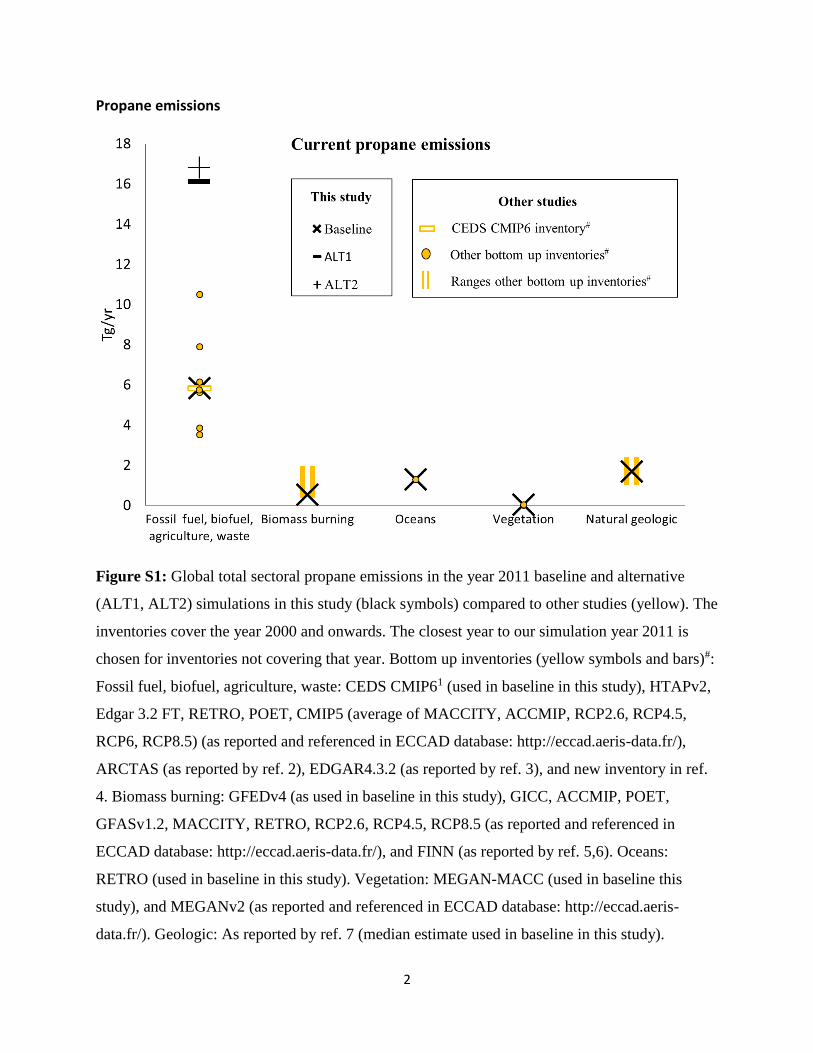
Propane emissions

Figure S1: Global total sectoral propane emissions in the year 2011 baseline and alternative

(ALT1, ALT2) simulations in this study (black symbols) compared to other studies (yellow). The

inventories cover the year 2000 and onwards. The closest year to our simulation year 2011 is

chosen for inventories not covering that year. Bottom up inventories (yellow symbols and bars)#:

Fossil fuel, biofuel, agriculture, waste: CEDS CMIP61 (used in baseline in this study), HTAPv2,

Edgar 3.2 FT, RETRO, POET, CMIP5 (average of MACCITY, ACCMIP, RCP2.6, RCP4.5,

RCP6, RCP8.5) (as reported and referenced in ECCAD database: http://eccad.aeris-data.fr/),

ARCTAS (as reported by ref. 2), EDGAR4.3.2 (as reported by ref. 3), and new inventory in ref.

4. Biomass burning: GFEDv4 (as used in baseline in this study), GICC, ACCMIP, POET,

GFASv1.2, MACCITY, RETRO, RCP2.6, RCP4.5, RCP8.5 (as reported and referenced in

ECCAD database: http://eccad.aeris-data.fr/), and FINN (as reported by ref. 5,6). Oceans:

RETRO (used in baseline in this study). Vegetation: MEGAN-MACC (used in baseline this

study), and MEGANv2 (as reported and referenced in ECCAD database: http://eccad.aeris-

data.fr/). Geologic: As reported by ref. 7 (median estimate used in baseline in this study).

3

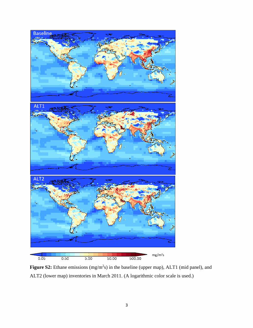
Figure S2: Ethane emissions (mg/m2s) in the baseline (upper map), ALT1 (mid panel), and

ALT2 (lower map) inventories in March 2011. (A logarithmic color scale is used.)

4

Sensitivity studies preindustrial conditions

Sensitivity simulations with meteorological input data for a different year and an alternative

inventory for biomass burning emissions (see Methods) resulted in similar Antarctic

concentrations and identical (meteorological sensitivity simulation) and 15 % lower (biomass

burning sensitivity simulation) inter-polar ratio.

5

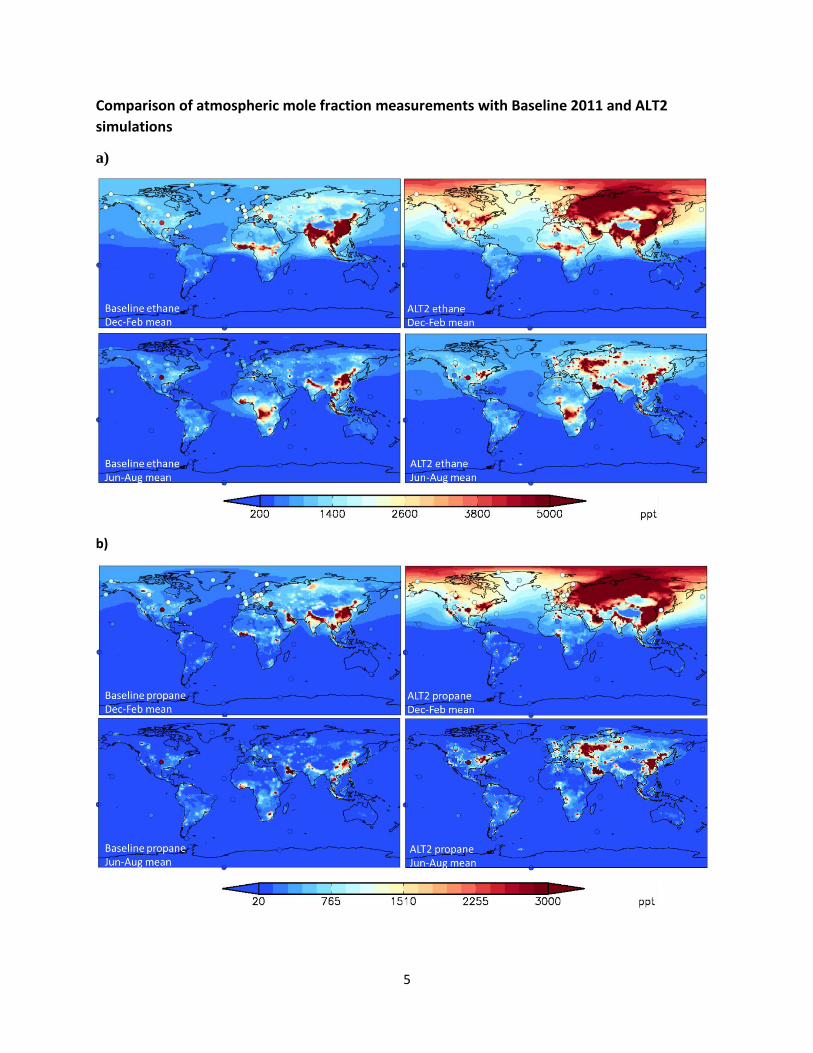
Comparison of atmospheric mole fraction measurements with Baseline 2011 and ALT2

simulations

a)

b)

6

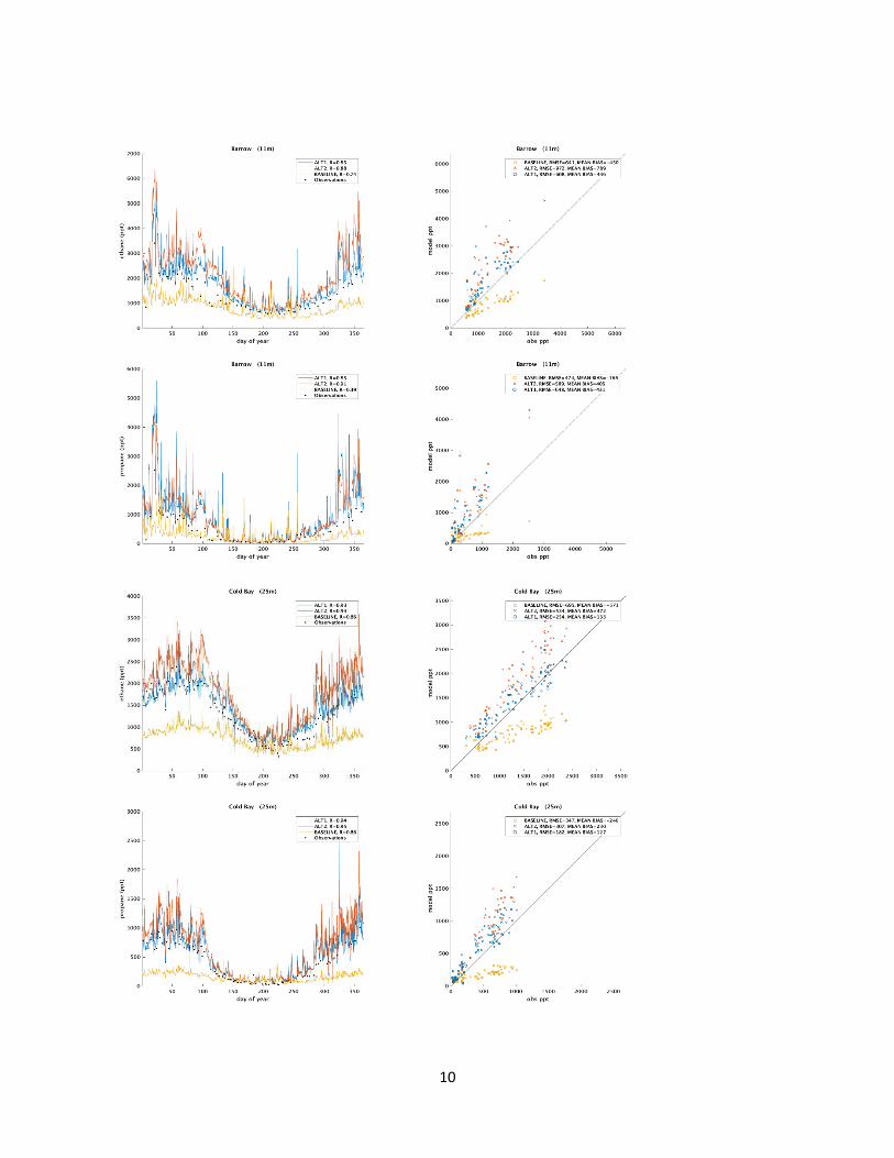
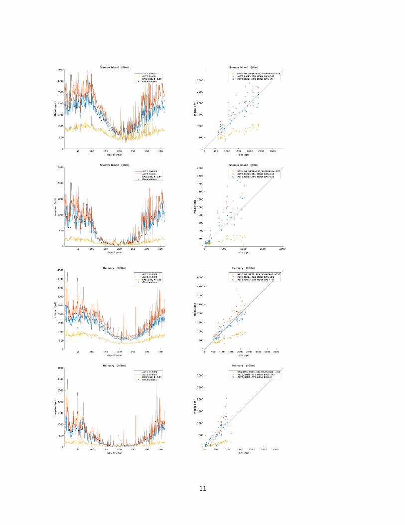
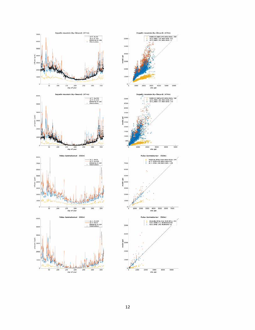
Figure S3: Comparison of modeled (background colours) and observed (colour-filled circles)

surface ethane (ppt) for the year 2011. Model data for the lowest model layer was used. Stations

with less than 6 samples within the 3 month averaging period were excluded from the

comparison. Mountain stations that typically sample free tropospheric air and that are situated in

areas where the model resolution doesnt resolve the terrain were also excluded. Details on the

applied observation datasets are found in the Methods section. b) Same for propane.

7

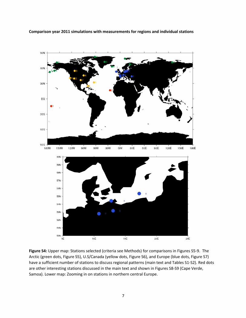
Comparison year 2011 simulations with measurements for regions and individual stations

Figure S4: Upper map: Stations selected (criteria see Methods) for comparisons in Figures S5-9. The

Arctic (green dots, Figure S5), U.S/Canada (yellow dots, Figure S6), and Europe (blue dots, Figure S7)

have a sufficient number of stations to discuss regional patterns (main text and Tables S1-S2). Red dots

are other interesting stations discussed in the main text and shown in Figures S8-S9 (Cape Verde,

Samoa). Lower map: Zooming in on stations in northern central Europe.

8

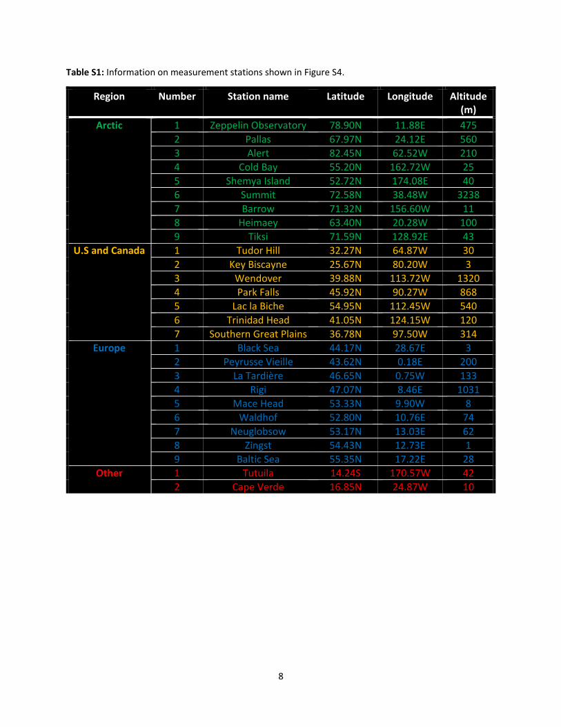
Table S1: Information on measurement stations shown in Figure S4.

Region Number Station name Latitude Longitude Altitude (m)

Arctic 1 Zeppelin Observatory 78.90N 11.88E 475

2 Pallas 67.97N 24.12E 560

3 Alert 82.45N 62.52W 210

4 Cold Bay 55.20N 162.72W 25

5 Shemya Island 52.72N 174.08E 40

6 Summit 72.58N 38.48W 3238

7 Barrow 71.32N 156.60W 11

8 Heimaey 63.40N 20.28W 100

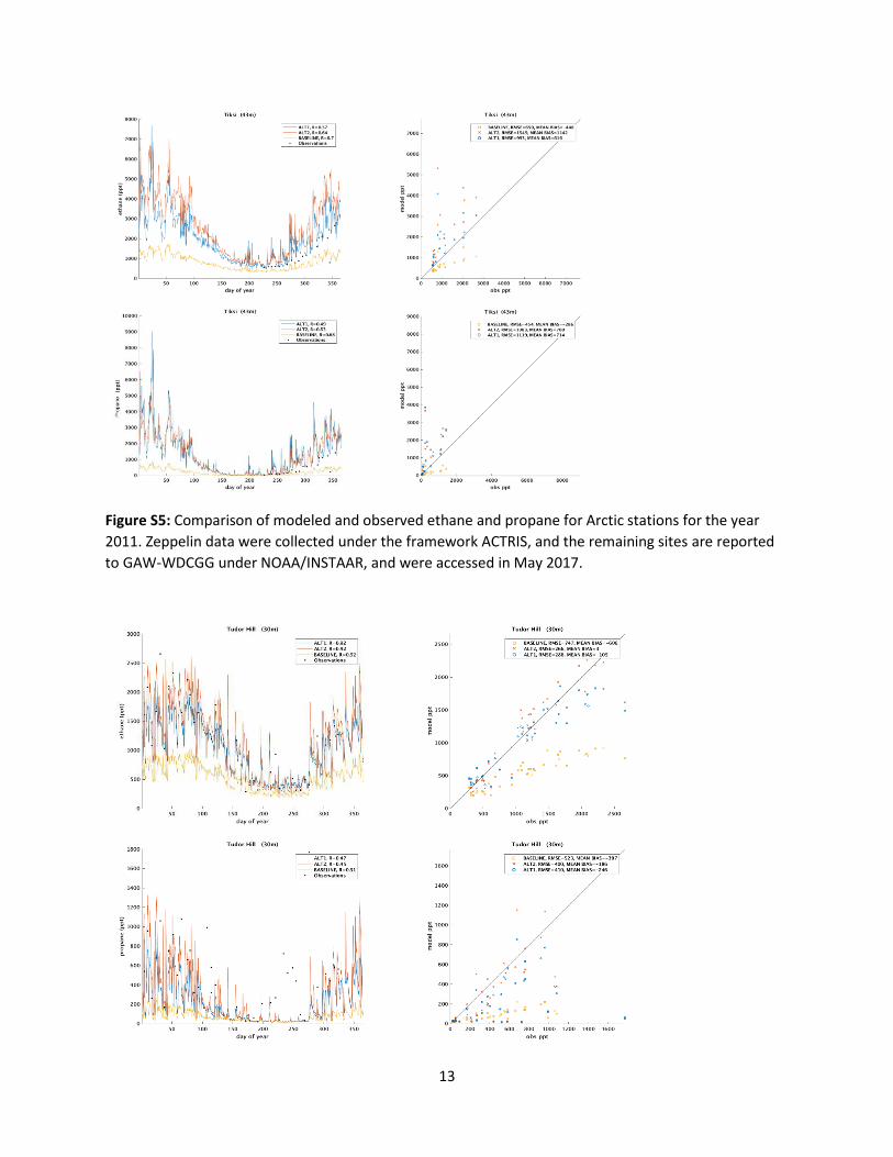
9 Tiksi 71.59N 128.92E 43

U.S and Canada 1 Tudor Hill 32.27N 64.87W 30

2 Key Biscayne 25.67N 80.20W 3

3 Wendover 39.88N 113.72W 1320

4 Park Falls 45.92N 90.27W 868

5 Lac la Biche 54.95N 112.45W 540

6 Trinidad Head 41.05N 124.15W 120

7 Southern Great Plains 36.78N 97.50W 314

Europe 1 Black Sea 44.17N 28.67E 3

2 Peyrusse Vieille 43.62N 0.18E 200

3 La Tardire 46.65N 0.75W 133

4 Rigi 47.07N 8.46E 1031

5 Mace Head 53.33N 9.90W 8

6 Waldhof 52.80N 10.76E 74

7 Neuglobsow 53.17N 13.03E 62

8 Zingst 54.43N 12.73E 1

9 Baltic Sea 55.35N 17.22E 28

Other 1 Tutuila 14.24S 170.57W 42

2 Cape Verde 16.85N 24.87W 10

9

10

11

12

13

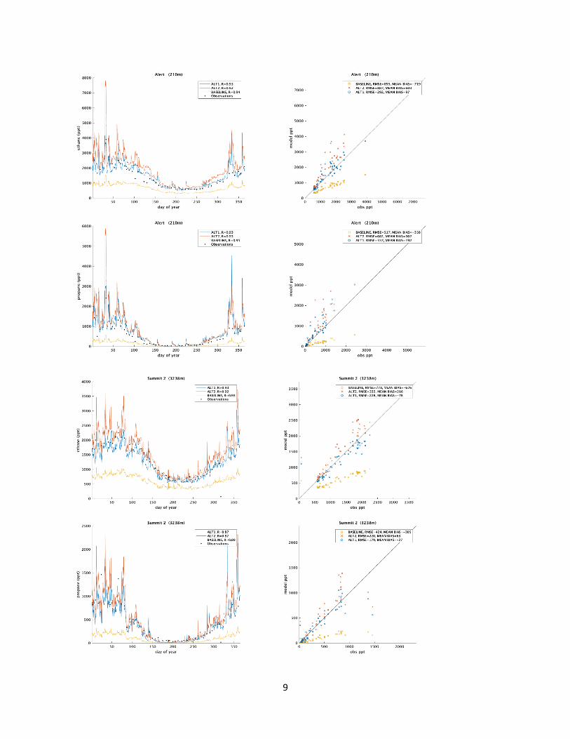
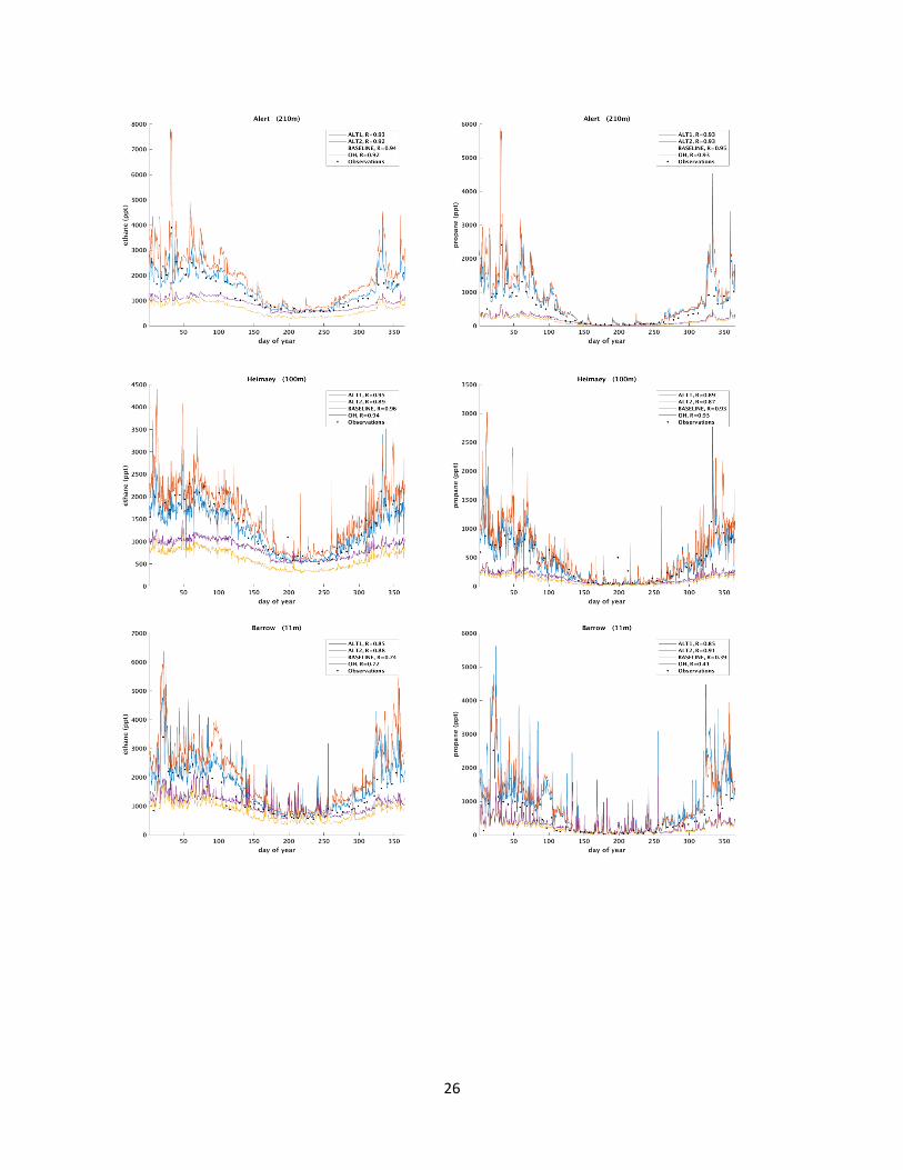
Figure S5: Comparison of modeled and observed ethane and propane for Arctic stations for the year

2011. Zeppelin data were collected under the framework ACTRIS, and the remaining sites are reported

to GAW-WDCGG under NOAA/INSTAAR, and were accessed in May 2017.

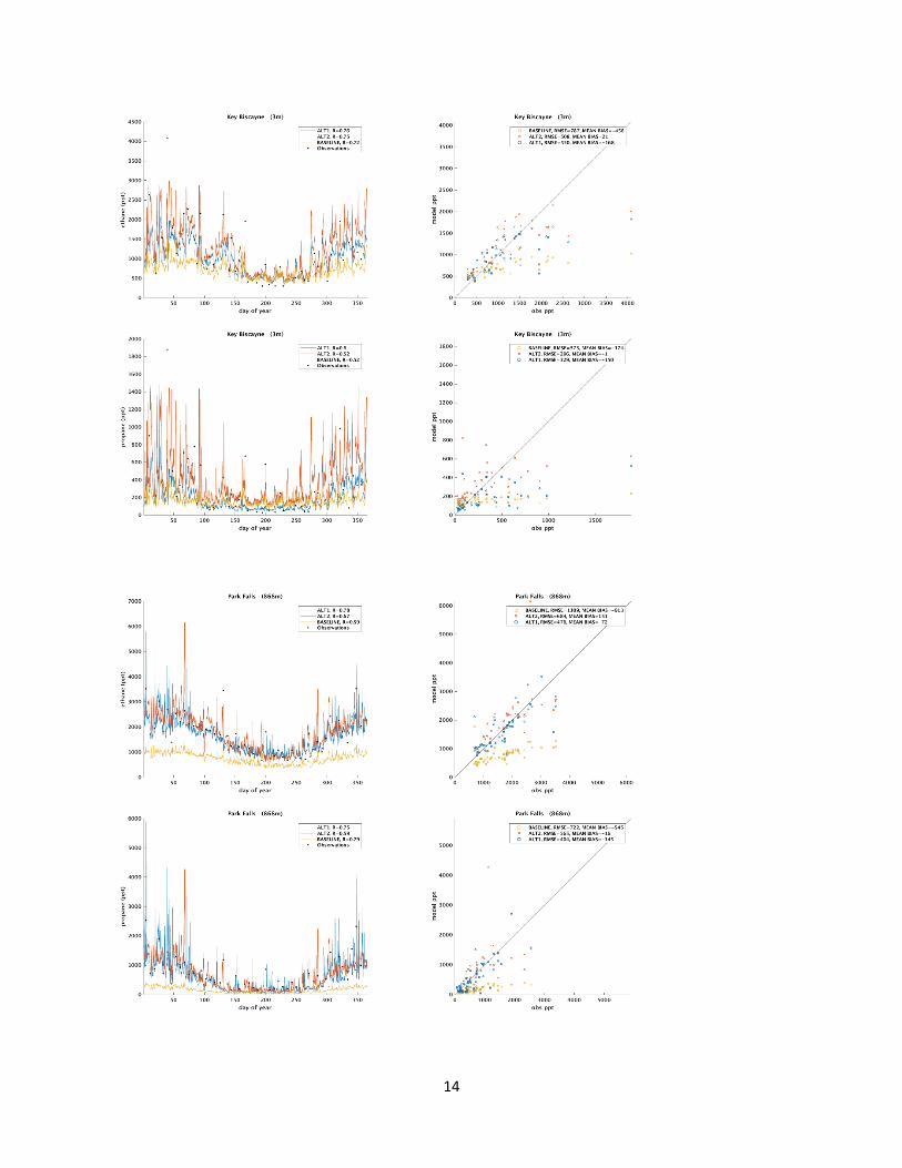
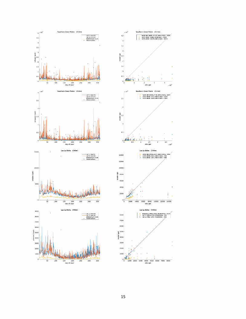
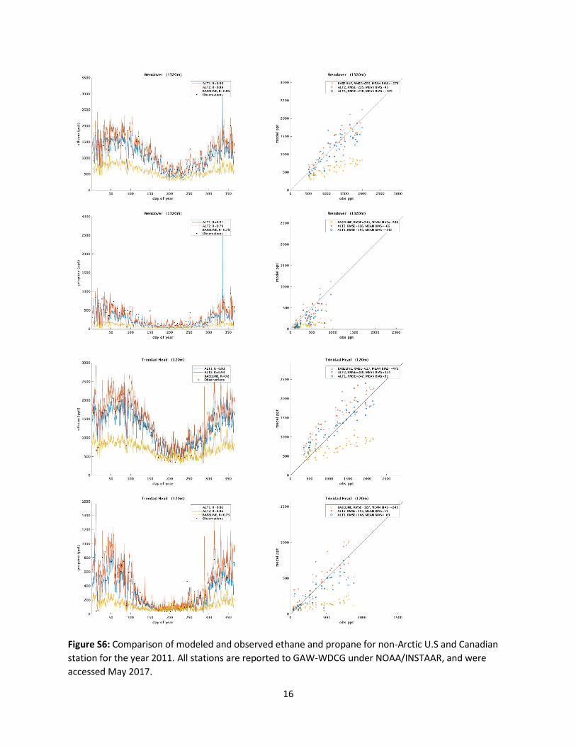
14

15

16

Figure S6: Comparison of modeled and observed ethane and propane for non-Arctic U.S and Canadian

station for the year 2011. All stations are reported to GAW-WDCG under NOAA/INSTAAR, and were

accessed May 2017.

17

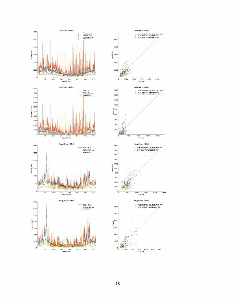
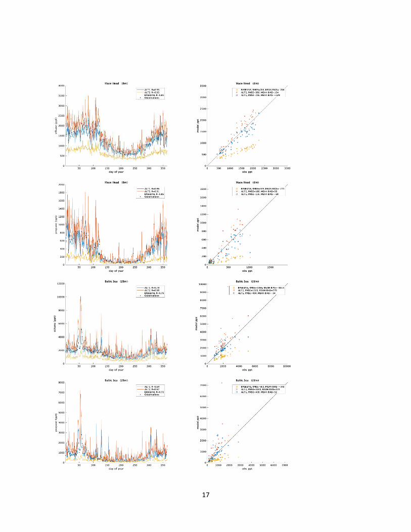
18

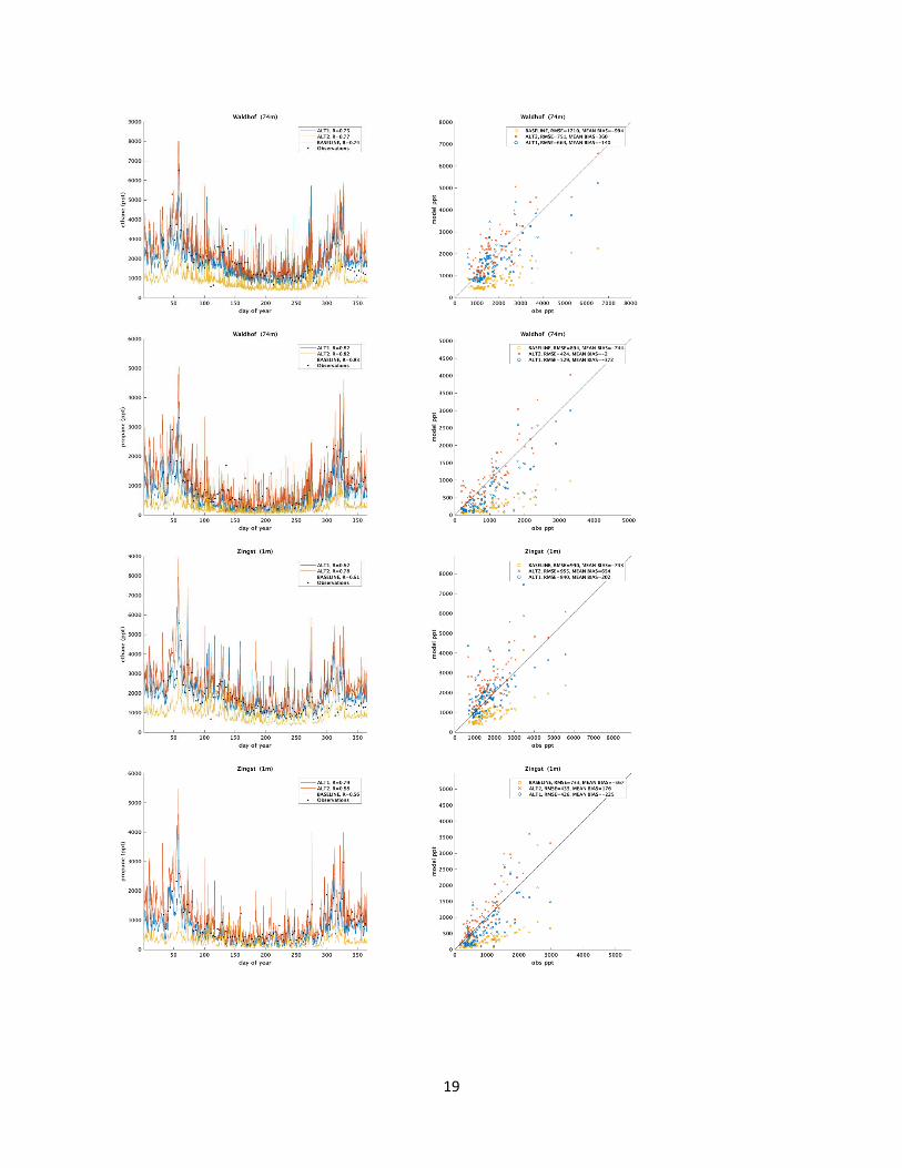
19

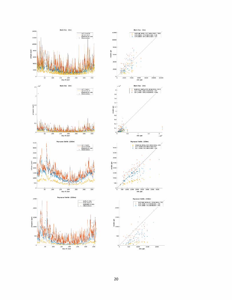
20

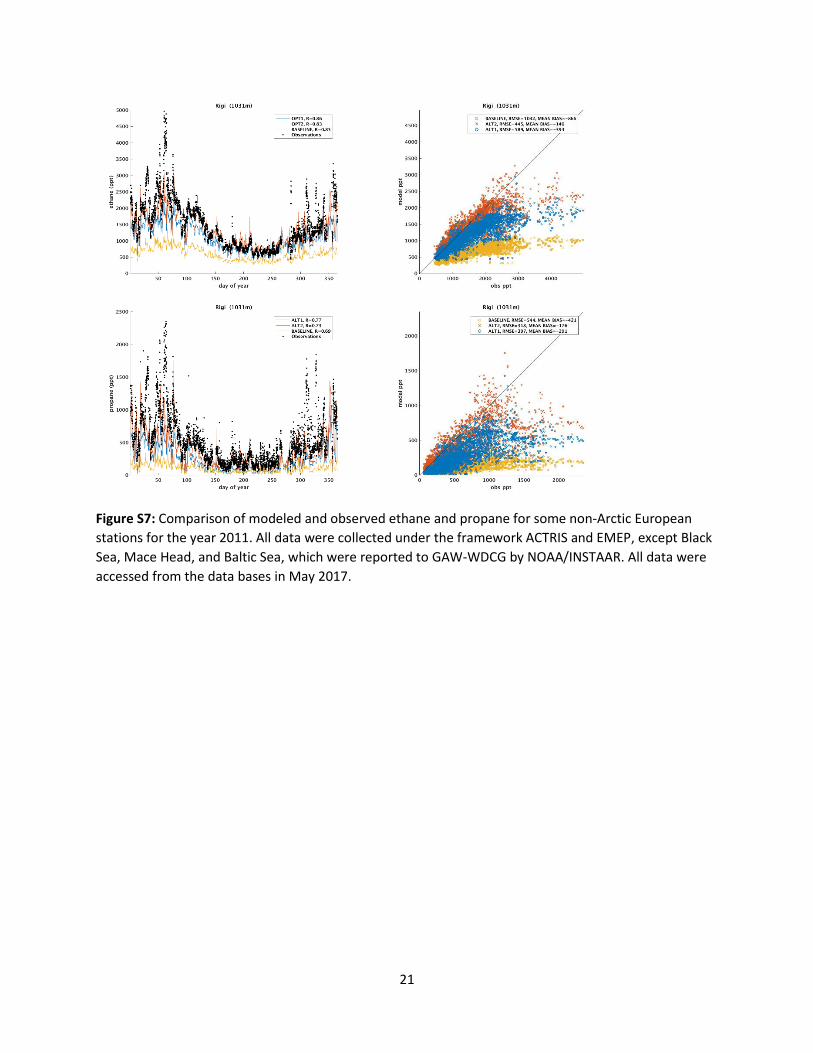
21

Figure S7: Comparison of modeled and observed ethane and propane for some non-Arctic European

stations for the year 2011. All data were collected under the framework ACTRIS and EMEP, except Black

Sea, Mace Head, and Baltic Sea, which were reported to GAW-WDCG by NOAA/INSTAAR. All data were

accessed from the data bases in May 2017.

22

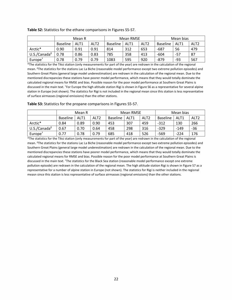
Table S2: Statistics for the ethane comparisons in Figures S5-S7.

Mean R Mean RMSE Mean bias

Baseline ALT1 ALT2 Baseline ALT1 ALT2 Baseline ALT1 ALT2

Arctic* 0.90 0.91 0.91 814 312 653 -687 56 479

U.S./Canada 0.78 0.86 0.83 785 358 413 -604 -57 87

Europe 0.78 0.79 0.79 1083 595 920 -879 -93 567 *The statistics for the Tiksi station (only measurements for part of the year) are redrawn in the calculation of the regional

mean. The statistics for the stations Lac La Biche (reasonable model performance except two extreme pollution episodes) and

Southern Great Plains (general large model underestimation) are redrawn in the calculation of the regional mean. Due to the

mentioned discrepancies these stations have poorer model performance, which means that they would totally dominate the

calculated regional means for RMSE and bias. Possible reason for the poor model performance at Southern Great Plains is

discussed in the main text. For Europe the high altitude station Rigi is shown in Figure S6 as a representative for several alpine

station in Europe (not shown). The statistics for Rigi is not included in the regional mean since this station is less representative

of surface airmasses (regional emissions) than the other stations.

Table S3: Statistics for the propane comparisons in Figures S5-S7.

Mean R Mean RMSE Mean bias

Baseline ALT1 ALT2 Baseline ALT1 ALT2 Baseline ALT1 ALT2

Arctic* 0.84 0.89 0.90 453 307 459 -312 130 266

U.S./Canada 0.67 0.70 0.64 458 298 316 -329 -149 -36

Europe 0.77 0.78 0.79 685 418 526 -569 -224 176 *The statistics for the Tiksi station (only measurements for part of the year) are redrawn in the calculation of the regional

mean. The statistics for the stations Lac La Biche (reasonable model performance except two extreme pollution episodes) and

Southern Great Plains (general large model underestimation) are redrawn in the calculation of the regional mean. Due to the

mentioned discrepancies these stations have poorer model performance, which means that they would totally dominate the

calculated regional means for RMSE and bias. Possible reason for the poor model performance at Southern Great Plains is

discussed in the main text. The statistics for the Black Sea station (reasonable model performance except one extreme

pollution episode) are redrawn in the calculation of the regional mean. The high altitude station Rigi is shown in Figure S7 as a

representative for a number of alpine station in Europe (not shown). The statistics for Rigi is neither included in the regional

measn since this station is less representative of surface airmasses (regional emissions) than the other stations.

23

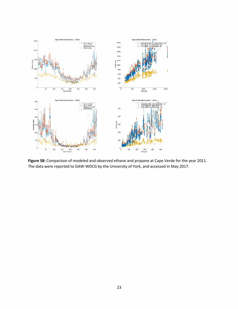
Figure S8: Comparison of modeled and observed ethane and propane at Cape Verde for the year 2011.

The data were reported to GAW-WDCG by the University of York, and accessed in May 2017.

24

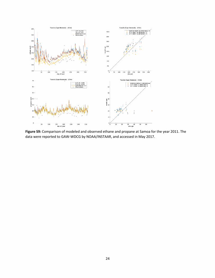
Figure S9: Comparison of modeled and observed ethane and propane at Samoa for the year 2011. The

data were reported to GAW-WDCG by NOAA/INSTAAR, and accessed in May 2017.

25

OH sensitivity study

26

27

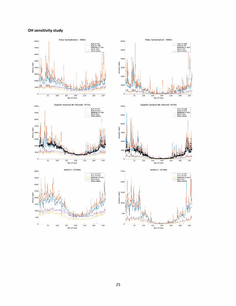
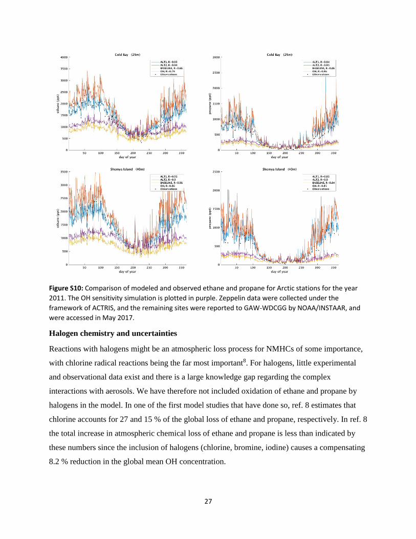
Figure S10: Comparison of modeled and observed ethane and propane for Arctic stations for the year

2011. The OH sensitivity simulation is plotted in purple. Zeppelin data were collected under the

framework of ACTRIS, and the remaining sites were reported to GAW-WDCGG by NOAA/INSTAAR, and

were accessed in May 2017.

Halogen chemistry and uncertainties

Reactions with halogens might be an atmospheric loss process for NMHCs of some importance,

with chlorine radical reactions being the far most important8. For halogens, little experimental

and observational data exist and there is a large knowledge gap regarding the complex

interactions with aerosols. We have therefore not included oxidation of ethane and propane by

halogens in the model. In one of the first model studies that have done so, ref. 8 estimates that

chlorine accounts for 27 and 15 % of the global loss of ethane and propane, respectively. In ref. 8

the total increase in atmospheric chemical loss of ethane and propane is less than indicated by

these numbers since the inclusion of halogens (chlorine, bromine, iodine) causes a compensating

8.2 % reduction in the global mean OH concentration.

28

Uncertainties in baseline and alternative anthropogenic emission inventories

Complete quantitative uncertainty estimates do not currently exist for the CEDS CMIP6

inventory1 used in our baseline simulation. In CEDS CMIP61 the uncertainties in global total

anthropogenic CO2 and SO2 emissions are estimated to be around 10 %, whereas they typically

are 100 % for carbonaceous aerosols. The emission uncertainties for CO, NOx, and NMHCs are

stated to be in between these numbers. Based on that, we assume an emission uncertainty of

60 % for anthropogenic emissions of ethane and propane in the CEDS CMIP6 inventory used in

our baseline simulations. This agrees quite well with the estimates for the older EDGARv3

(http://themasites.pbl.nl/tridion/en/themasites/edgar/documentation/uncertainties/index-2.html),

where the uncertainties for individual sectors fall in the categories medium (around 50 %) and

high (around 100 %). Based on the span in the approximate uncertainty numbers reported in

CEDS CMIP61 and EDGAR (above link to documentation) we further assume that our selected

CEDS CMIP6 uncertainty estimate ( 60 %) has a confidence level of one standard deviation

(68 %).

There are very few quantitative datasets available on uncertainties in other global standard

community emission inventories. It is therefore difficult to estimate the combined uncertainty for

the eight other inventories shown in Figures 1b, S1 and S11. We expect the emission

uncertainties in each of these older inventories to be equal or larger than that of the CEDS

CMIP6 state of the art inventory.

For the new fugitive fossil fuel emission dataset in the ALT1 inventory the uncertainty in

emissions from associated gas flow and handling is based on the uncertainty estimates in Table 3

of ref. 9. For the uncertainty in emissions from unintended leakage, IPCC default factors10 were

modified to -50% of the IPCC low-end and to +10% of the IPCC high-end. The ranges for the

IPCC default factors are very large, in particular the high-end value for developing countries,

which is likely to reflect emissions from occasional "super-emitters", that are hardly

representative for the global scale. The uncertainty range for leakage during shale gas extraction

was set to be from 2% to 5%. For coal emissions the low and high estimates of ref. 11 is used.

The overall uncertainty range for the ALT1 fugitive fossil fuel emissions is -28 % to +38 % for

both ethane and propane with a confidence level of one standard deviation (68 %).

29

The ALT2 inventory emission uncertainties for the fugitive fossil fuel emissions are from ref. 11.

Based on top down studies12 the low gas scenario from ref. 11 is considered most likely. Our

upper total fugitive emission estimate uses the combination emissions low gas and high coal and

oil, while our lower total fugitive emission estimate has the combination low gas, coal, and oil.

The overall uncertainty in the fugitive fuel emissions in ALT2 range from -27 % to +30 % for

both ethane and propane with a confidence level of one standard deviation (68 %).

In the fugitive fossil fuel datasets in the ALT1 and ALT2 inventories the relative uncertainties

(around 30 %) are about halved compared to that assumed ( 60 %) above for the CEDS

CMIP6 inventory. The reason is that the ALT1 and ALT2 datasets are based on novel

approaches to quantify and attribute methane and NMHC emissions and take much better into

account that the emission factors from venting and flaring of associated gas released during

extraction vary considerably across different oil, coal and gas fields in the world. The main text

and methods section provide further information on differences in data quality, calculation

methods, etc.

In the ALT1 and ALT2 simulations we use conservative low estimates of fugitive fossil fuel

emissions. Due to potential double-counting11 we assume full overlap with geologic seepage

emissions: Conservative low estimates = Best estimates with geologic seepage emissions

subtracted (see Methods for details). The anthropogenic (excluding biomass burning) ethane

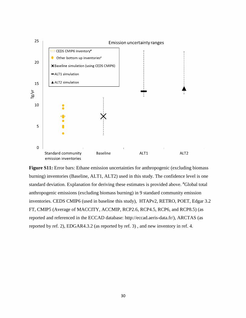
emissions used in the baseline, ALT1, and ALT2 model simulations are shown in Figure S11

together with uncertainty ranges calculated based on the estimates discussed in this section.

30

Figure S11: Error bars: Ethane emission uncertainties for anthropogenic (excluding biomass

burning) inventories (Baseline, ALT1, ALT2) used in this study. The confidence level is one

standard deviation. Explanation for deriving these estimates is provided above. #Global total

anthropogenic emissions (excluding biomass burning) in 9 standard community emission

inventories. CEDS CMIP6 (used in baseline this study), HTAPv2, RETRO, POET, Edgar 3.2

FT, CMIP5 (Average of MACCITY, ACCMIP, RCP2.6, RCP4.5, RCP6, and RCP8.5) (as

reported and referenced in the ECCAD database: http://eccad.aeris-data.fr/), ARCTAS (as

reported by ref. 2), EDGAR4.3.2 (as reported by ref. 3) , and new inventory in ref. 4.

31

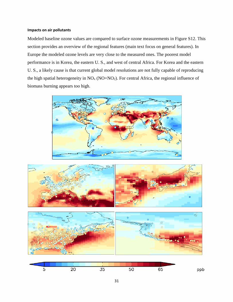
Impacts on air pollutants

Modeled baseline ozone values are compared to surface ozone measurements in Figure S12. This

section provides an overview of the regional features (main text focus on general features). In

Europe the modeled ozone levels are very close to the measured ones. The poorest model

performance is in Korea, the eastern U. S., and west of central Africa. For Korea and the eastern

U. S., a likely cause is that current global model resolutions are not fully capable of reproducing

the high spatial heterogeneity in NOx (NO+NO2). For central Africa, the regional influence of

biomass burning appears too high.

32

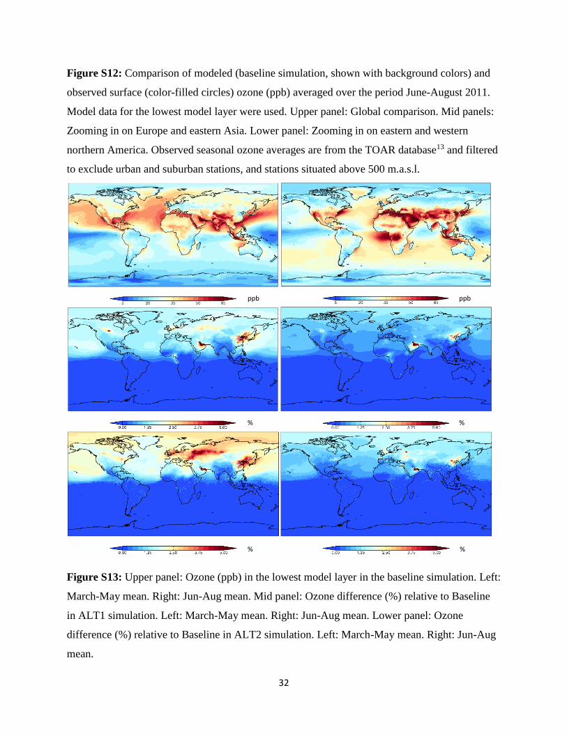
Figure S12: Comparison of modeled (baseline simulation, shown with background colors) and

observed surface (color-filled circles) ozone (ppb) averaged over the period June-August 2011.

Model data for the lowest model layer were used. Upper panel: Global comparison. Mid panels:

Zooming in on Europe and eastern Asia. Lower panel: Zooming in on eastern and western

northern America. Observed seasonal ozone averages are from the TOAR database13 and filtered

to exclude urban and suburban stations, and stations situated above 500 m.a.s.l.

Figure S13: Upper panel: Ozone (ppb) in the lowest model layer in the baseline simulation. Left:

March-May mean. Right: Jun-Aug mean. Mid panel: Ozone difference (%) relative to Baseline

in ALT1 simulation. Left: March-May mean. Right: Jun-Aug mean. Lower panel: Ozone

difference (%) relative to Baseline in ALT2 simulation. Left: March-May mean. Right: Jun-Aug

mean.

1

2

3

ppb ppb

% %

% %

33

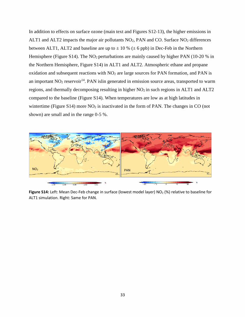
In addition to effects on surface ozone (main text and Figures S12-13), the higher emissions in

ALT1 and ALT2 impacts the major air pollutants NO2, PAN and CO. Surface NO2 differences

between ALT1, ALT2 and baseline are up to 10 % ( 6 ppb) in Dec-Feb in the Northern

Hemisphere (Figure S14). The NO2 perturbations are mainly caused by higher PAN (10-20 % in

the Northern Hemisphere, Figure S14) in ALT1 and ALT2. Atmospheric ethane and propane

oxidation and subsequent reactions with NO2 are large sources for PAN formation, and PAN is

an important NO2 reservoir14. PAN islin generated in emission source areas, transported to warm

regions, and thermally decomposing resulting in higher NO2 in such regions in ALT1 and ALT2

compared to the baseline (Figure S14). When temperatures are low as at high latitudes in

wintertime (Figure S14) more NO2 is inactivated in the form of PAN. The changes in CO (not

shown) are small and in the range 0-5 %.

Figure S14: Left: Mean Dec-Feb change in surface (lowest model layer) NO2 (%) relative to baseline for

ALT1 simulation. Right: Same for PAN.

NO2 PAN

34

References

1 Hoesly, R. M. et al. Historical (17502014) anthropogenic emissions of reactive gases and aerosols from the Community Emission Data System (CEDS). Geosci. Model Dev. Discuss. 2017, 1-41 (2017).

2 Emmons, L. K. et al. The POLARCAT Model Intercomparison Project (POLMIP): overview and evaluation with observations. Atmos. Chem. Phys. 15, 6721-6744 (2015).

3 Huang, G. et al. Speciation of anthropogenic emissions of non-methane volatile organic compounds: a global gridded data set for 19702012. Atmos. Chem. Phys. 17, 7683-7701 (2017).

4 Tzompa-Sosa, Z. A. et al. Revisiting global fossil fuel and biofuel emissions of ethane. Journal of Geophysical Research: Atmospheres 122, 2493-2512 (2017).

5 Helmig, D. et al. Reversal of global atmospheric ethane and propane trends largely due to US oil and natural gas production. Nature Geosci 9, 490-495 (2016).

6 Franco, B. et al. Evaluating ethane and methane emissions associated with the development of oil and natural gas extraction in North America. Environmental Research Letters 11, 044010 (2016).

7 Etiope, G. & Ciccioli, P. Earth's Degassing: A Missing Ethane and Propane Source. Science 323, 478-478 (2009).

8 Sherwen, T. et al. Global impacts of tropospheric halogens (Cl, Br, I) on oxidants and composition in GEOS-Chem, Atmos. Chem. Phys. 16, 12239-12271 (2016).

9 Hglund-Isaksson, L. Bottom-up simulations of methane and ethane emissions from global oil and gas sysreftems 1980 to 2012. Environmental Research Letters 12, 024007 (2017).

10 IPCC. Vol. 2 IPCC Guidelines for National Greenhouse Gas Inventories Tables 4.2.4 and 4.2.5 (IPCC, Japan, 2006).

11 Schwietzke, S., Griffin, W. M., Matthews, H. S. & Bruhwiler, L. M. P. Global Bottom-Up Fossil Fuel Fugitive Methane and Ethane Emissions Inventory for Atmospheric Modeling. ACS Sustainable Chemistry & Engineering 2, 1992-2001 (2014).

12 Schwietzke, S., Griffin, W. M., Matthews, H. S. & Bruhwiler, L. M. P. Natural Gas Fugitive Emissions Rates Constrained by Global Atmospheric Methane and Ethane. Environ. Sci. Technol. 48, 7714-7722 (2014).

13 Schultz, M. G. et al. in Supplement to: Schultz, MG et al. (in press): Tropospheric Ozone Assessment Report: Database and Metrics Data of Global Surface Ozone Observations. Elementa, https://doi.org/10.1525/elementa.244 Custom 8 (PANGAEA, 2017).

14 Fischer, E. V. et al. Atmospheric peroxyacetyl nitrate (PAN): a global budget and source attribution. Atmos. Chem. Phys. 14, 2679-2698 (2014).