Discrepancy Analysis of State Sequences

Matthias Studer, Gilbert Ritschard,Alexis Gabadinho and Nicolas S. Muller

University of Geneva, Switzerland

Article to appear in Sociological Methods & Research in August 2011

Abstract

In this article we define a methodological framework for analyzing the relationship between statesequences and covariates. Inspired by the ANOVA principles, our approach looks at how the covariatesexplain the discrepancy of the sequences. We use the pairwise dissimilarities between sequences todetermine the discrepancy which makes it then possible to develop a series of statistical-significance-based analysis tools. We introduce generalized simple and multi-factor discrepancy-based methodsto test for differences between groups, a pseudo R2 for measuring the strength of sequence–covariateassociations, a generalized Levene statistic for testing differences in the within-group discrepancies, aswell as tools and plots for studying the evolution of the differences along the timeframe and a regressiontree method for discovering the most significant discriminant covariates and their interactions. Inaddition, we extend all methods to account for case weights. The scope of the proposed methodologicalframework is illustrated using a real-world sequence dataset.

Keywords: distance, dissimilarities, analysis of variance, regression tree, tree structured ANOVA,state sequence, optimal matching, homogeneity in discrepancies, Levene test, permutation test.

Author’s note: Please address correspondence to Matthias Studer, Institute for Demographic and LifeCourse Studies, University of Geneva, Bvd Pont D’Arve 40, 1211 Geneva 4, Switzerland, Matthias.

Studer@unige.ch. All the numerical results and plots presented in this article can be reproduced withthe R script provided as a supplemental file on the website of the journal.

1

1 Introduction

Optimal matching (OM) and, more generally, clustering of state sequences have become popular tools foranalyzing life trajectories since their initial introduction in the social sciences in the late 1980s (Abbottand Forrest 1986; Abbott and Hrycak 1990). The popularity of these techniques is largely attributableto the holistic view they provide on the life course construction process. As emphasized by Billari (2005)such an approach considers the complete life sequence as a single unit of analysis, as opposed to eventhistory analysis, for instance, which focuses on specific events of the life process such as marriage or thestart of a new job.

In general, the OM approach consists of measuring the pairwise dissimilarities between sequencesand then using the obtained values in an unsupervised clustering algorithm to build a typology of theobserved sequences (i.e., to find homogeneous groups of sequences). Such analysis has proven to be aneffective exploratory tool for discovering the main characteristics of a set of sequences without formulatingany a-priori hypothesis. Further, it permits identification of typical trajectories and recurring structuresin the sequences, thus bringing out fundamental descriptive information and making the data easier tocomprehend. From a sociological point of view, groups determined by clustering techniques are usefulfor characterizing typical trajectories. Even more, it is often assumed that cases in a cluster all followmore or less an associated ideal type of trajectory. Clustering serves in this way for identifying the idealtypes, which then in turn provide nice, simplified interpretations of the clusters.

Aside the understanding of the intrinsic characteristics of the sequences, in this article, we are in-terested in how the individual sequences are impacted by their context. A common practice in thatperspective is to investigate the relationship of the identified sequence types—the clusters—with covari-ates such as sex and birth cohort. This is achieved, for example, by looking at the association between thecluster membership and the covariates, or by explaining cluster membership by means of logistic regres-sions or classification trees. The downside of this cluster-based approach, however, is that by representingthe diversity of trajectories with a limited number of clusters, one inevitably loses the information aboutthe diversity within each cluster. In the causal perspective, reducing the set of sequences to a limitednumber of standard trajectories is a too-crude approximation and would lead to considering deviationsfrom the standard inside a cluster as non-explained error terms. Furthermore, knowledge of the clustermembership alone does not inform about the distances and differences between clusters. As a result,wrong conclusions may be drawn about the sequences–covariates relationships.

As a solution to this problem, we propose a set of methods—the discrepancy analysis—that allow todirect analysis of the sequence–covariate links (i.e., without any prior clustering). Our approach focuseson the discrepancy of the sequences, which we measure from their pairwise dissimilarities (OM distances,for example). This trick allows then a generalization of the ANOVA principles. The basic idea behindthe ANOVA approach is to measure and test the part of the discrepancy among sequences that can beexplained by covariates. For instance, one can assess what fraction of the differences between individuals’academic careers can be explained by sex or how the construction of one’s familial life may differ accordingto social origin.

The article is organized as follows. In Section 2, we briefly review the relevant literature, and inSection 3 we describe the dataset on the transition from school to work used for illustrating the discussedmethods. In Section 4 we introduce a dissimilarity-based measure of discrepancy for a set of possiblyweighted sequences and discuss its interpretation. In Section 5 we propose methods to study the relation-ship between sequences and a single categorical variable; that is, we focus on the comparison of groupsof sequences defined according to the levels of a given covariate. We derive a pseudo R2 for measuringthe share of sequence discrepancy explained by the grouping variable and introduce a pseudo F test forassessing the significance of the association. We extend both statistics to account for case weights. Wepropose also a Levene-like statistic for testing the homogeneity of within-group sequence discrepancies.To conclude the section, we illustrate the behavior of the statistics with simulations. In Section 6, weshow how results can be further investigated and rendered to characterize the differences between groups.Section 7 deals with the multi-factor case for which we introduce original formulas that can account forcase weights. Section 8 exploits the previous material in a tree-structured fashion to reveal the factorsthat best discriminate sequences. Finally, in Section 9, we provide a brief overview on how to apply thepresented methods in R with our TraMineR package.

To avoid overloading the reader, detailed mathematical developments and discussions have been taken

2

out of the main text and included in Appendices A to C.

2 Literature review

Several approaches have been used to study the association between objects described by their pairwisedissimilarities and a categorical covariate (Gower and Krzanowski 1999; Anderson 2001; McArdle andAnderson 2001; Mielke and Berry 2007; Cuadras 2008). Apart from the most popular ones, whichgenerally adopt ANOVA/MANOVA principles, Mielke and Berry (1983, 2007) have suggested using adhoc statistics based on sums of distances. Reiss, Stevens, Shehzad, Petkova, and Milham (2009) showthat the two approaches are equivalent under certain conditions. The statistical significance of theassociation is generally assessed through permutation tests, although Mielke and Berry (2007) propose aparameterized approximation for the empirical distribution generated by the permutations. All of theseauthors consider only metric distances. In contrast, McArdle and Anderson (2001) extend the sameapproach to semi-metric dissimilarities. This latter solution can also be applied in a multi-factor case. Asfar as weights are concerned, an interesting contribution one finds in the literature is the paper of Delicado(2007), who accounts for weights with a test derived from Gower and Krzanowski’s (1999) formulationfor the single factor case.

The different methods are used in various domains such as genetics (Zapala and Schork 2006), thestudy of income density functions (Delicado 2007), or the study of neuroimaging data (Reiss et al. 2009).Gower and Krzanowski (1999) deal with situations where the number of dependent (response) variablesis larger than the number of observations. In line with the work by McArdle and Anderson (2001), themain application field is ecology and especially the analysis of ecosystems by means of semi-metrics, suchas that of Bray-Curtis. To the best of our knowledge, however, ANOVA-like tools have not yet beenapplied so far to life trajectory analysis.

The methods presented in this article are inspired from the work of Mielke and Berry (2007) andMcArdle and Anderson (2001). We adapt their solutions for the study of state sequences in the socialsciences and extend them, so that we can also account for case weights. We also complement the theo-retical background of their approaches with notions such as the contribution to discrepancy derived fromBatagelj’s (1988) developments of the Ward criterion.

The analysis of differences in discrepancies between groups (i.e., the test of equality in within-groupdiscrepancies) has rarely been considered for dissimilarity-based discrepancies. Anderson (2006) proposestwo tests based on distances in an associated principal coordinate space. Studer, Ritschard, Gabadinho,and Muller (2010) consider a generalization of Bartlett’s test that uses directly the original dissimilarities.The latter approach is not suitable, however, for weighted data.

Regarding tree-structured methods, there are only few recent attempts to apply them on objectscharacterized by their dissimilarities. Piccarreta and Billari (2007) propose a non-supervised dissimilarity-based divisive tree algorithm that grows the tree independently of any covariates. They applied it onsequence data. Similarly to the present paper, Geurts, Wehenkel, and d’Alche Buc (2006) propose theuse of a kernel-based supervised method; however, their approach is limited to Euclidean distances. Amore general dissimilarity-based method can be found in Piccarreta (2010). Unlike our proposal, her tree-growing method is not controlled by a statistical significance and therefore requires post-pruning. Thetree algorithm considered in Section 8 is essentially the same as the one introduced by Studer, Ritschard,Gabadinho, and Muller (2009) and Studer et al. (2010). Here, we build on it and adapt it for weighteddata.

3 Illustrative data set

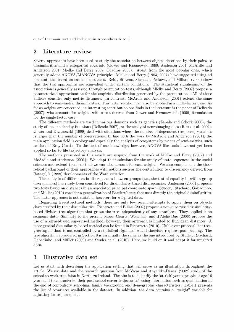
Let us start with describing the application setting that will serve as an illustration throughout thearticle. We use data and the research question from McVicar and Anyadike-Danes’ (2002) study of theschool-to-work transition in Northern Ireland. The aim is to “identify the ‘at-risk’ young people at age 16years and to characterize their post-school career trajectories” using information such as qualification atthe end of compulsory schooling, family background and demographic characteristics. Table 1 presentsthe list of covariates available in the dataset. In addition, the data contains a “weight” variable foradjusting for response bias.

3

Table 1. List of Covariates

Variable Description Values

sex Gender female, maleregion Location of school in North Ireland Belfast, North Eastern,

South Eastern, Southern, Westernreligion Religion Catholic, Protestantfunemp Father unemployed at time of survey yes, nofmpr Father has a professional, managerial or related job yes, nolivboth Living with both parents at time of first sweep of survey yes, nogrammar Grammar school secondary eduction yes, nogcse5eq Qualifications gained by the end of compulsory education:

5 or more GCSEs at grades A–C, or equivalent yes, no

4 Discrepancy of a set of sequences

In this section, we define a measure of the discrepancy of a set of sequences. In a life course framework, thediscrepancy measures the between-individual variability of the life trajectories. Therefore, higher discrep-ancy, for example, would reflect a greater level of uncertainty about the path followed by the individuals.Depending on the situations, such uncertainty may be interpreted either as a form of precariousness or,on the contrary, as a reflection of the multiplicity of choices the individuals face. The discrepancy conceptconsidered here must be clearly distinguished from the within-individual longitudinal state diversity thatcan be measured with the longitudinal entropy (Widmer and Ritschard 2009), the turbulence (Elzinga2010), or the complexity index (Gabadinho, Ritschard, Studer, and Muller 2010). The latter measurethe diversity of states and transitions inside sequences, while the discrepancy assesses the diversity of thetrajectories.

Aside from this diversity interpretation, the discrepancy is also the key concept for measuring theassociation between sequences and covariates. Decomposing it into explained between-groups and residualwithin-groups discrepancy permits measurement of the explained share of discrepancy and testing fordifferences between groups. These topics will be addressed in the next sections.

Since we cannot directly observe the distance to some “mean sequence”, the discrepancy of sequenceswill be defined from their pairwise dissimilarities. There are many different ways of computing suchdissimilarities, either through proximity measures counting common characteristics (Elzinga 2007) orusing edit distances (Lesnard 2010). The most popular dissimilarity measure used for sequence analysisin the social sciences is the optimal matching (OM) edit distance, also known as generalized Levenshteindistance in computer science. It is defined as the lowest cost of transforming one sequence into the otherby means of state insertions–deletions (indel) and state substitutions. The total transformation costdepends on the individual cost of each used operation. Those costs can be organized into an augmentedsubstitution cost-matrix between states by considering each insertion–deletion as a substitution with anull element (i.e., by defining a row and a column for this null element).1 The resulting OM distancesatisfies surely the triangle inequality as long as the elements of this augmented substitution cost matrixverify it (Yujian and Bo 2007). When that is not the case, the resulting OM dissimilarity betweentwo sequences x and y could be greater than the sum of their dissimilarities with some other sequence.Though we will use the OM distance with the costs defined in McVicar and Anyadike-Danes (2002) forour application example, the way of measuring the discrepancy described hereafter is in no way limitedto the OM distance alone. Any other measure of dissimilarity between sequences could be used instead.

The presentation in the remainder of the section is based on the generalization of the Ward criterionmade by Batagelj (1988). The concepts introduced may also be found in Anderson (2001), Reiss et al.(2009) and Mielke and Berry (2007), though these papers deal only with the unweighed case while wepropose here formulas that account for weights as well.

1Though this definition permits state dependent insertion–deletion costs, unique indel costs are most often used.

4

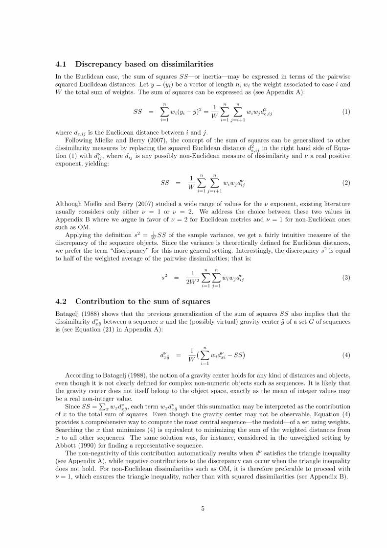
4.1 Discrepancy based on dissimilarities

In the Euclidean case, the sum of squares SS—or inertia—may be expressed in terms of the pairwisesquared Euclidean distances. Let y = (yi) be a vector of length n, wi the weight associated to case i andW the total sum of weights. The sum of squares can be expressed as (see Appendix A):

SS =

n∑i=1

wi(yi − y)2 =1

W

n∑i=1

n∑j=i+1

wiwjd2e,ij (1)

where de,ij is the Euclidean distance between i and j.Following Mielke and Berry (2007), the concept of the sum of squares can be generalized to other

dissimilarity measures by replacing the squared Euclidean distance d2e,ij in the right hand side of Equa-tion (1) with dνij , where dij is any possibly non-Euclidean measure of dissimilarity and ν a real positiveexponent, yielding:

SS =1

W

n∑i=1

n∑j=i+1

wiwjdνij (2)

Although Mielke and Berry (2007) studied a wide range of values for the ν exponent, existing literatureusually considers only either ν = 1 or ν = 2. We address the choice between these two values inAppendix B where we argue in favor of ν = 2 for Euclidean metrics and ν = 1 for non-Euclidean onessuch as OM.

Applying the definition s2 = 1W SS of the sample variance, we get a fairly intuitive measure of the

discrepancy of the sequence objects. Since the variance is theoretically defined for Euclidean distances,we prefer the term “discrepancy” for this more general setting. Interestingly, the discrepancy s2 is equalto half of the weighted average of the pairwise dissimilarities; that is:

s2 =1

2W 2

n∑i=1

n∑j=1

wiwjdνij (3)

4.2 Contribution to the sum of squares

Batagelj (1988) shows that the previous generalization of the sum of squares SS also implies that thedissimilarity dνxg between a sequence x and the (possibly virtual) gravity center g of a set G of sequencesis (see Equation (21) in Appendix A):

dνxg =1

W

( n∑i=1

widνxi − SS

)(4)

According to Batagelj (1988), the notion of a gravity center holds for any kind of distances and objects,even though it is not clearly defined for complex non-numeric objects such as sequences. It is likely thatthe gravity center does not itself belong to the object space, exactly as the mean of integer values maybe a real non-integer value.

Since SS =∑x wxd

νxg, each term wxd

νxg under this summation may be interpreted as the contribution

of x to the total sum of squares. Even though the gravity center may not be observable, Equation (4)provides a comprehensive way to compute the most central sequence—the medoid—of a set using weights.Searching the x that minimizes (4) is equivalent to minimizing the sum of the weighted distances fromx to all other sequences. The same solution was, for instance, considered in the unweighed setting byAbbott (1990) for finding a representative sequence.

The non-negativity of this contribution automatically results when dν satisfies the triangle inequality(see Appendix A), while negative contributions to the discrepancy can occur when the triangle inequalitydoes not hold. For non-Euclidean dissimilarities such as OM, it is therefore preferable to proceed withν = 1, which ensures the triangle inequality, rather than with squared dissimilarities (see Appendix B).

5

5 Comparing groups of sequences

Aside from evaluating the variability of a set of sequences, measuring discrepancy from pairwise dis-similarities permits generalization of the analysis of variance (ANOVA) principles to any dissimilaritymeasure. It allows computation of the share of discrepancy “explained” by a covariate and thus eval-uation of the strength of the association between trajectories and a covariate. Although classical testsbased on normality assumptions are not applicable in this case, the significance of the relation can beassessed through permutation tests, as discussed in Anderson (2001).

In Section 5.3, we introduce a new test to compare group discrepancy. In some situations, it maybe of interest to test whether the discrepancies within groups differ significantly. We then discuss theinterpretation and the visualization of the difference between state sequences. In the last subsection, weprovide empirical insights on the behavior of the proposed tests with simulations.

5.1 Measuring association

When generalizing the notion of sum of squares to non-Euclidean measures of dissimilarity, the Huygenstheorem (Equation 5) that states that the total sum of squares (SST ) is the between sum of squares(SSB) plus the residual within sum of squares (SSW ) remains valid (Batagelj 1988).

SST = SSB + SSW (5)

Thus, we can apply the ANOVA machinery to sequence objects.All terms in Equation (5) can be derived from formula (2). The total sum of squares (SST ) and the

within sum of squares (SSW ) are computed directly with formula (2), SSW being simply the sum of thewithin sums of squares of each subgroup. The between sum of squares SSB is then obtained by taking thedifference between SST and SSW . Using Equation (5), we can assess the share of discrepancy explainedby a categorical or discretized continuous variable. In the spirit of ANOVA, this reduction of discrepancyis due to a difference in the positioning of the gravity centers gk of the classes k (Batagelj 1988). Hence,conceptually, we look for the part of the discrepancy that is explained by differences in group positioning,and we measure it with the R2 formula (6). Alternatively, we may consider the F that compares theexplained discrepancy to the residual discrepancy. The F formula is provided in Equation (7), where mis the number of groups.

R2 =SSBSST

(6)

F =SSB/(m− 1)

SSW /(W −m)(7)

5.2 Assessing statistical significance

The statistical significance of the association (i.e., of the explained part of the discrepancy) cannotbe assessed with Fisher’s F distribution as in classical ANOVA.2 The F statistic (7) does not followa Fisher distribution with sequence objects for which the normality assumption is hardly defendable.Therefore, we consider a permutation test (Anderson 2001; Manly 2007) which works as follows. Ateach step we change the group—the value of the covariates—assigned to each sequence by means of arandomly chosen permutation of the group membership vector. We thus get an Fperm value for eachpermutation. Repeating this operation R times, we obtain an empirical non-parametric distribution of Fthat characterizes its distribution under independence (i.e., assuming the sequences are assigned to thecases independently of the explanatory factors). From this distribution, we can assess the significance ofthe observed Fobs statistic by means of the proportion of Fperm that are higher than Fobs. It is generallyadmitted that 5,000 permutations should be used to assess a significance threshold of 1% and 1,000 fora threshold of 5% (see Manly 2007, and Appendix C).

The issue is how we can or even if we should adapt such permutation tests to account for weights.We propose three solutions:

2We have also considered the use of the Brown-Forsythe F ∗ statistic to account for unequal group discrepancy (Brownand Forsythe 1974b). However, in our experiments results were always almost the same as with the traditional F . For sakeof simplicity, we do not develop further this option.

6

1. Replicate cases a number of times corresponding to the weights before performing the permutation.This approach supposes that weights are integer counts.

2. Replace at each step the simple permutation with a random assignment of covariate profiles to thesequences using distributions defined by the weights.

3. Proceed with permutations ignoring weights and use them for computing the statistics for eachpermutation.

When the weights stand for counts of aggregated cases, we should restore individual cases by replicatingthe aggregated ones. By permuting aggregates only, we would miss possible permutations of cases withinaggregated groups and therefore end up with a less powerful test. The second option is more or lessequivalent but can be used with non-integer weights. Both of these techniques assume that weights reflectan aggregation of independently drawn cases. However, when weights do not result from aggregation butare intended to improve the sample representativeness, as it is the case in the example mvad data, itwould not be correct to replicate cases. For example, a weight of 4 would not mean that 4 cases weredrawn, and hence replicating it 4 times would incorrectly inflate the sample size.

Thus, the first and the second solutions should be used with counts reflecting aggregation. The thirdone should be applied in cases where weights are aimed at improving the sample representativeness.

0 2 4 6 8 10 12

0.0

0.2

0.4

0.6

Live with both parents

Pseudo F

Den

sity

Statistic: 2.49 (P−value: 0.2092 )

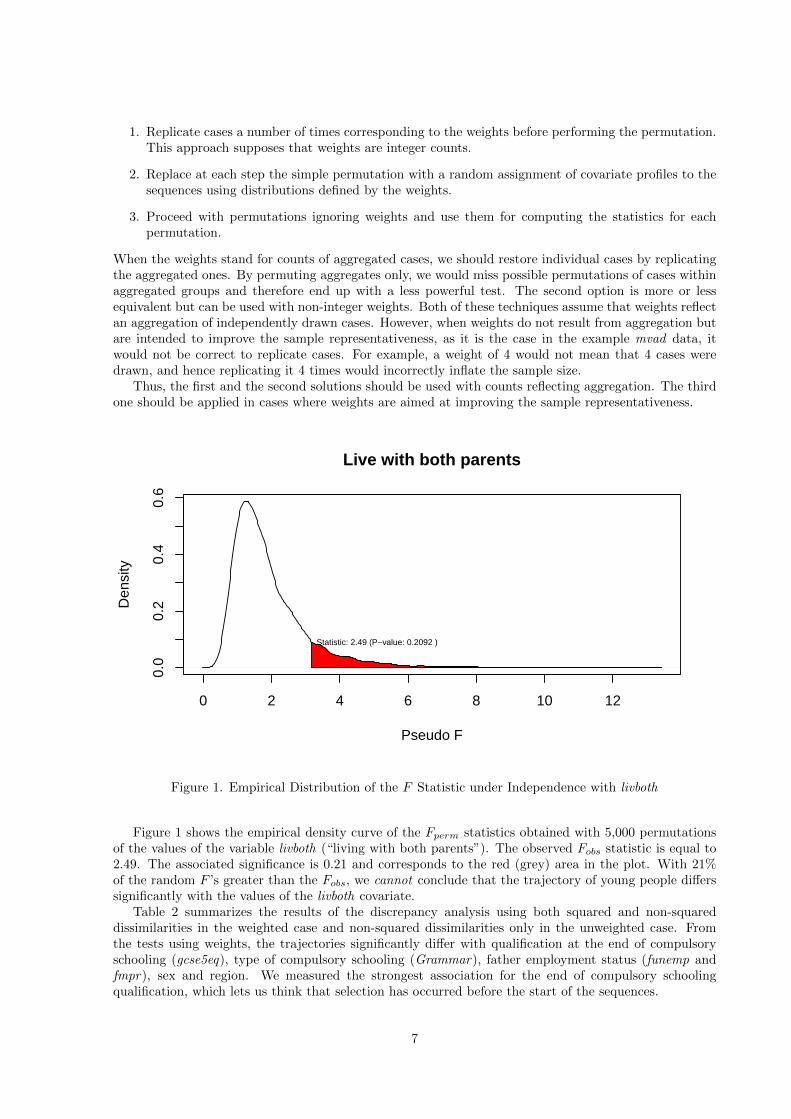
Figure 1. Empirical Distribution of the F Statistic under Independence with livboth

Figure 1 shows the empirical density curve of the Fperm statistics obtained with 5,000 permutationsof the values of the variable livboth (“living with both parents”). The observed Fobs statistic is equal to2.49. The associated significance is 0.21 and corresponds to the red (grey) area in the plot. With 21%of the random F ’s greater than the Fobs, we cannot conclude that the trajectory of young people differssignificantly with the values of the livboth covariate.

Table 2 summarizes the results of the discrepancy analysis using both squared and non-squareddissimilarities in the weighted case and non-squared dissimilarities only in the unweighted case. Fromthe tests using weights, the trajectories significantly differ with qualification at the end of compulsoryschooling (gcse5eq), type of compulsory schooling (Grammar), father employment status (funemp andfmpr), sex and region. We measured the strongest association for the end of compulsory schoolingqualification, which lets us think that selection has occurred before the start of the sequences.

7

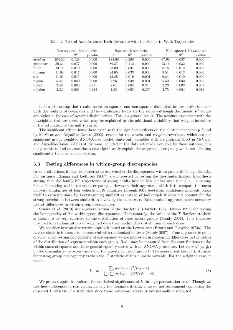
Table 2. Test of Association of Each Covariate with the School-to-Work Trajectories

Non-squared dissimilarity Squared dissimilarity Non-squared, UnweightedF R2 p-value F R2 p-value F R2 p-value

gcse5eq 104.09 0.128 0.000 184.09 0.206 0.000 67.69 0.087 0.000grammar 59.34 0.077 0.000 89.87 0.112 0.000 23.16 0.032 0.000fmpr 13.72 0.019 0.000 23.00 0.031 0.000 8.76 0.012 0.000funemp 11.98 0.017 0.000 24.05 0.033 0.000 9.51 0.013 0.000sex 11.03 0.015 0.000 13.85 0.019 0.001 6.84 0.010 0.000region 5.44 0.030 0.000 7.26 0.039 0.001 5.50 0.030 0.000livboth 2.49 0.003 0.211 2.61 0.004 0.240 2.23 0.003 0.033religion 2.32 0.003 0.234 1.88 0.003 0.365 2.75 0.004 0.014

It is worth noting that results based on squared and non-squared dissimilarities are quite similar—both the ranking of covariates and the significance levels are the same—although the pseudo R2 valuesare higher in the case of squared dissimilarities. This is a general result. The p-values associated with theunweighted test are lower, which may be explained by the additional variability that weights introducein the estimation of the null F curve.

The significant effects found here agree with the significant effects on the cluster membership foundby McVicar and Anyadike-Danes (2002), except for the livboth and religion covariates, which are notsignificant in our weighted ANOVA-like model. Since only variables with a significant effect in McVicarand Anyadike-Danes’ (2002) study were included in the data set made available by those authors, it isnot possible to find out covariates that significantly explain the sequence discrepancy while not affectingsignificantly the cluster membership.

5.3 Testing differences in within-group discrepancies

In some situations, it may be of interest to test whether the discrepancies within groups differ significantly.For instance, Elzinga and Liefbroer (2007) are interested in testing the de-standardization hypothesisstating that the family life trajectories of young adults become less similar over time (i.e., in testingfor an increasing within-cohort discrepancy). However, their approach, which is to compare the meanpairwise similarities of four cohorts in 19 countries through 90% bootstrap confidence intervals, lendsitself to criticism since by bootstrapping similarities instead of individuals it does not account for thestrong correlation between similarities involving the same case. Better suited approaches are necessaryto test differences in within-group discrepancies.

Studer et al. (2010) use a generalization of the Bartlett T (Bartlett 1937; Jobson 1991) for testingthe homogeneity of the within-group discrepancies. Unfortunately, the value of the T Bartlett statisticis known to be very sensitive to the distribution of cases across groups (Manly 2007). It is thereforeunsuited for randomizations of weighted data that modify this distribution at each draw.

We consider here an alternative approach based on the Levene test (Brown and Forsythe 1974a). TheLevene statistic is known to be powerful with randomization tests (Manly 2007). From a geometric pointof view, when testing homogeneity of discrepancy we are interested in measuring differences in the radiusof the distribution of sequences within each group. Radii may be measured from the contributions to thewithin sums of squares and their general equality tested with an ANOVA procedure. Let zi` = dν(xi, g`)be the dissimilarity between case i and the gravity center of group `. The generalized Levene L statisticfor testing group homogeneity is then the F statistic of this numeric variable. For the weighted case, itreads:

L =

∑` w`(z` − z)2/(m− 1)∑

`

∑i wi(zi` − z`)2/(W −m)

(8)

We propose again to evaluate the statistical significance of L through permutation tests. Though wetest here differences in real values, namely the dissimilarities zi`’s, we do not recommend comparing theobserved L with the F distribution since those values are generally not normally distributed.

8

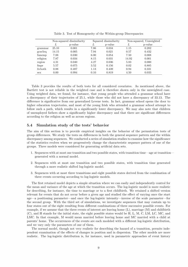
Table 3. Test of Homogeneity of the Within-group Discrepancies

Non-squared dissimilarity Squared dissimilarity Non-squared, UnweightedL p-value L p-value L p-value

grammar 25.10 0.001 7.86 0.034 1.15 0.282gcse5eq 14.15 0.005 7.94 0.021 0.57 0.432funemp 7.88 0.030 6.00 0.054 7.50 0.008religion 7.87 0.034 8.15 0.031 14.92 0.001region 4.31 0.040 4.27 0.036 5.83 0.000fmpr 5.57 0.075 3.52 0.156 0.02 0.885livboth 0.88 0.487 1.13 0.439 0.94 0.331sex 0.00 0.994 0.10 0.819 4.50 0.033

Table 3 provides the results of both tests for all considered covariates. As mentioned above, theBartlett test is not reliable in the weighted case and is therefore shown only in the unweighted case.Using weighted data, we found, for instance, that young people who attended a grammar school havea discrepancy of their trajectories of 25.1, while those who did not have a discrepancy of 33.13. Thedifference is significative from our generalized Levene tests. In fact, grammar school opens the door tohigher education trajectories, and most of the young Irish who attended a grammar school attempt tofollow such a path, which results in a significantly lower discrepancy. We may also note that childrenof unemployed fathers show a significantly higher discrepancy and that there are significant differencesaccording to the religion as well as across regions.

5.4 Simulation study of the tests’ behavior

The aim of this section is to provide empirical insights on the behavior of the permutation tests ofgroup differences. We study the tests on differences in both the general sequence pattern and the withindiscrepancy among sequences. We conducted a series of simulation studies to examine how the significanceof the statistics evolves when we progressively change the characteristic sequence pattern of one of thegroups. Three models were considered for generating artificial data sets.

1. Sequences with at most one transition and two possible states, with transition time—age at transition—generated with a normal model.

2. Sequences with at most one transition and two possible states, with transition time generatedthrough a more realistic shifted log-logistic model.

3. Sequences with at most three transitions and eight possible states derived from the combination ofthree events occurring according to log-logistic models.

The first retained model depicts a simple situation where we can easily and independently control forthe mean and variance of the age at which the transition occurs. The log-logistic model is more realisticfor describing, for instance, the time to marriage or to a first childbirth. We retained a shifted versionrelevant for events that do not occur before a given age and studied the effect of varying once the startage—a positioning parameter—and once the log-logistic intensity—inverse of the scale parameter—forthe second group. With the third set of simulations, we investigate sequences that may contain up tofour states out of the eight resulting from different combinations of three successive possible events. Forexample, if we assume that the three events of interest are leaving home (L), marriage (M) and childbirth(C), and H stands for the initial state, the eight possible states would be H, L, M, C, LM, LC, MC, andLMC. In that example, M would mean married before leaving home and MC married with a child atparents’ home. The occurrences of the events are each modeled with a different log-logistic distribution,and we vary only the parameters of one of them.

The normal model, though not very realistic for describing the hazard of a transition, permits inde-pendent examination of the effects of changes in position and in dispersion. The other models are morerealistic. The log-logistic distribution is, for instance, used in parametric approaches of event history

9

analysis (Blossfeld and Rohwer 2002). What makes it particularly interesting is that it allows for non-monotone risks. It is characterized by an intensity parameter λ and a shape parameter b. The inverse ofλ is known as the scale parameter, and it is also the median of the distribution. Hence, an increase in λreduces discrepancy but also changes the location. To control positioning independently of the discrep-ancy, we consider a start a parameter that specifies the threshold age where the log-logistic risk starts.The retained values for its b shape and λ intensity parameter are based on estimates obtained by Billari(2001b) in an analysis of age at first marriage in Italy. Finally, the last model considers multiple eventsand states that correspond typically to situations encountered in life course analysis as described above.

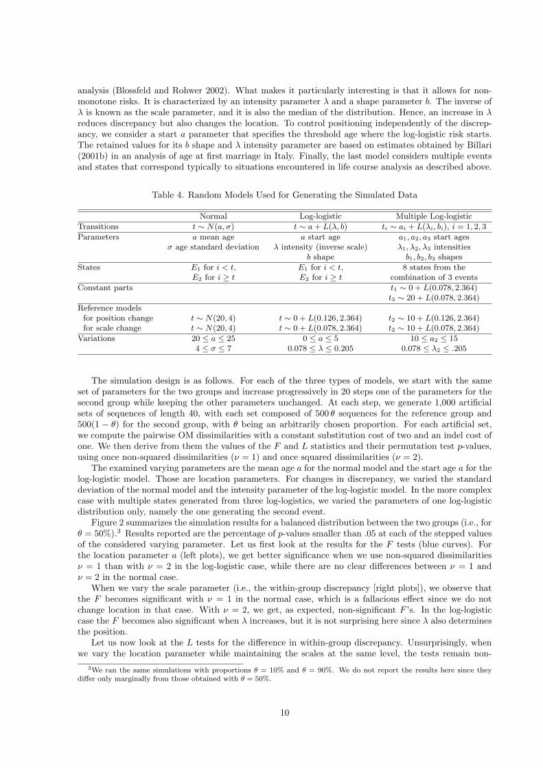
Table 4. Random Models Used for Generating the Simulated Data

Normal Log-logistic Multiple Log-logistic

Transitions t ∼ N(a, σ) t ∼ a+ L(λ, b) ti ∼ ai + L(λi, bi), i = 1, 2, 3

Parameters a mean age a start age a1, a2, a3 start agesσ age standard deviation λ intensity (inverse scale) λ1, λ2, λ3 intensities

b shape b1, b2, b3 shapes

States E1 for i < t, E1 for i < t, 8 states from theE2 for i ≥ t E2 for i ≥ t combination of 3 events

Constant parts t1 ∼ 0 + L(0.078, 2.364)t3 ∼ 20 + L(0.078, 2.364)

Reference modelsfor position change t ∼ N(20, 4) t ∼ 0 + L(0.126, 2.364) t2 ∼ 10 + L(0.126, 2.364)for scale change t ∼ N(20, 4) t ∼ 0 + L(0.078, 2.364) t2 ∼ 10 + L(0.078, 2.364)

Variations 20 ≤ a ≤ 25 0 ≤ a ≤ 5 10 ≤ a2 ≤ 154 ≤ σ ≤ 7 0.078 ≤ λ ≤ 0.205 0.078 ≤ λ2 ≤ .205

The simulation design is as follows. For each of the three types of models, we start with the sameset of parameters for the two groups and increase progressively in 20 steps one of the parameters for thesecond group while keeping the other parameters unchanged. At each step, we generate 1,000 artificialsets of sequences of length 40, with each set composed of 500 θ sequences for the reference group and500(1 − θ) for the second group, with θ being an arbitrarily chosen proportion. For each artificial set,we compute the pairwise OM dissimilarities with a constant substitution cost of two and an indel cost ofone. We then derive from them the values of the F and L statistics and their permutation test p-values,using once non-squared dissimilarities (ν = 1) and once squared dissimilarities (ν = 2).

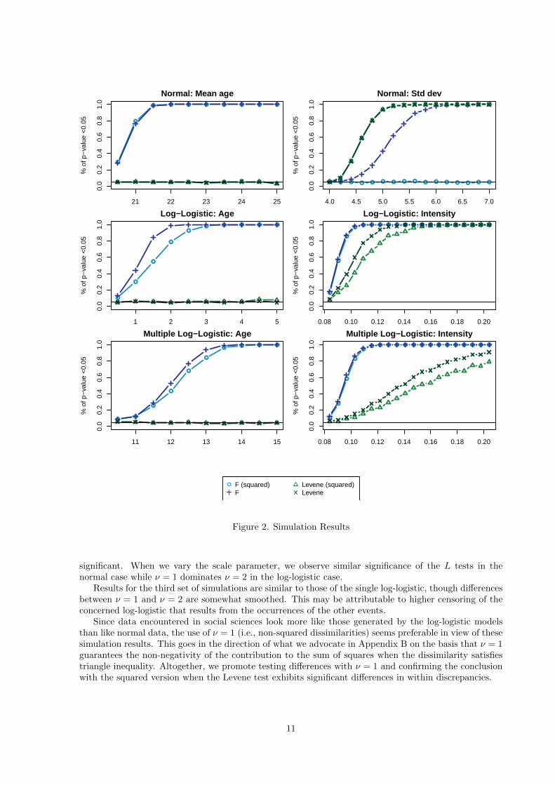
The examined varying parameters are the mean age a for the normal model and the start age a for thelog-logistic model. Those are location parameters. For changes in discrepancy, we varied the standarddeviation of the normal model and the intensity parameter of the log-logistic model. In the more complexcase with multiple states generated from three log-logistics, we varied the parameters of one log-logisticdistribution only, namely the one generating the second event.

Figure 2 summarizes the simulation results for a balanced distribution between the two groups (i.e., forθ = 50%).3 Results reported are the percentage of p-values smaller than .05 at each of the stepped valuesof the considered varying parameter. Let us first look at the results for the F tests (blue curves). Forthe location parameter a (left plots), we get better significance when we use non-squared dissimilaritiesν = 1 than with ν = 2 in the log-logistic case, while there are no clear differences between ν = 1 andν = 2 in the normal case.

When we vary the scale parameter (i.e., the within-group discrepancy [right plots]), we observe thatthe F becomes significant with ν = 1 in the normal case, which is a fallacious effect since we do notchange location in that case. With ν = 2, we get, as expected, non-significant F ’s. In the log-logisticcase the F becomes also significant when λ increases, but it is not surprising here since λ also determinesthe position.

Let us now look at the L tests for the difference in within-group discrepancy. Unsurprisingly, whenwe vary the location parameter while maintaining the scales at the same level, the tests remain non-

3We ran the same simulations with proportions θ = 10% and θ = 90%. We do not report the results here since theydiffer only marginally from those obtained with θ = 50%.

10

●

●

● ● ● ● ● ● ● ●

21 22 23 24 25

0.0

0.2

0.4

0.6

0.8

1.0

Normal: Mean age%

of p

−va

lue

<0.

05

● ● ● ● ● ● ● ● ● ● ● ● ● ● ● ●

4.0 4.5 5.0 5.5 6.0 6.5 7.0

0.0

0.2

0.4

0.6

0.8

1.0

Normal: Std dev

% o

f p−

valu

e <

0.05

●

●

●

●

●● ● ● ● ●

1 2 3 4 5

0.0

0.2

0.4

0.6

0.8

1.0

Log−Logistic: Age

% o

f p−

valu

e <

0.05

●

●

●

●● ● ● ● ● ● ● ● ● ● ● ● ● ● ● ●

0.08 0.10 0.12 0.14 0.16 0.18 0.20

0.0

0.2

0.4

0.6

0.8

1.0

Log−Logistic: Intensity

% o

f p−

valu

e <

0.05

●●

●

●

●

●

●● ● ●

11 12 13 14 15

0.0

0.2

0.4

0.6

0.8

1.0

Multiple Log−Logistic: Age

% o

f p−

valu

e <

0.05

●

●

●

●

●● ● ● ● ● ● ● ● ● ● ● ● ● ● ●

0.08 0.10 0.12 0.14 0.16 0.18 0.20

0.0

0.2

0.4

0.6

0.8

1.0

Multiple Log−Logistic: Intensity

% o

f p−

valu

e <

0.05

● F (squared)F

Levene (squared)Levene

Figure 2. Simulation Results

significant. When we vary the scale parameter, we observe similar significance of the L tests in thenormal case while ν = 1 dominates ν = 2 in the log-logistic case.

Results for the third set of simulations are similar to those of the single log-logistic, though differencesbetween ν = 1 and ν = 2 are somewhat smoothed. This may be attributable to higher censoring of theconcerned log-logistic that results from the occurrences of the other events.

Since data encountered in social sciences look more like those generated by the log-logistic modelsthan like normal data, the use of ν = 1 (i.e., non-squared dissimilarities) seems preferable in view of thesesimulation results. This goes in the direction of what we advocate in Appendix B on the basis that ν = 1guarantees the non-negativity of the contribution to the sum of squares when the dissimilarity satisfiestriangle inequality. Altogether, we promote testing differences with ν = 1 and confirming the conclusionwith the squared version when the Levene test exhibits significant differences in within discrepancies.

11

6 Studying and rendering group differences

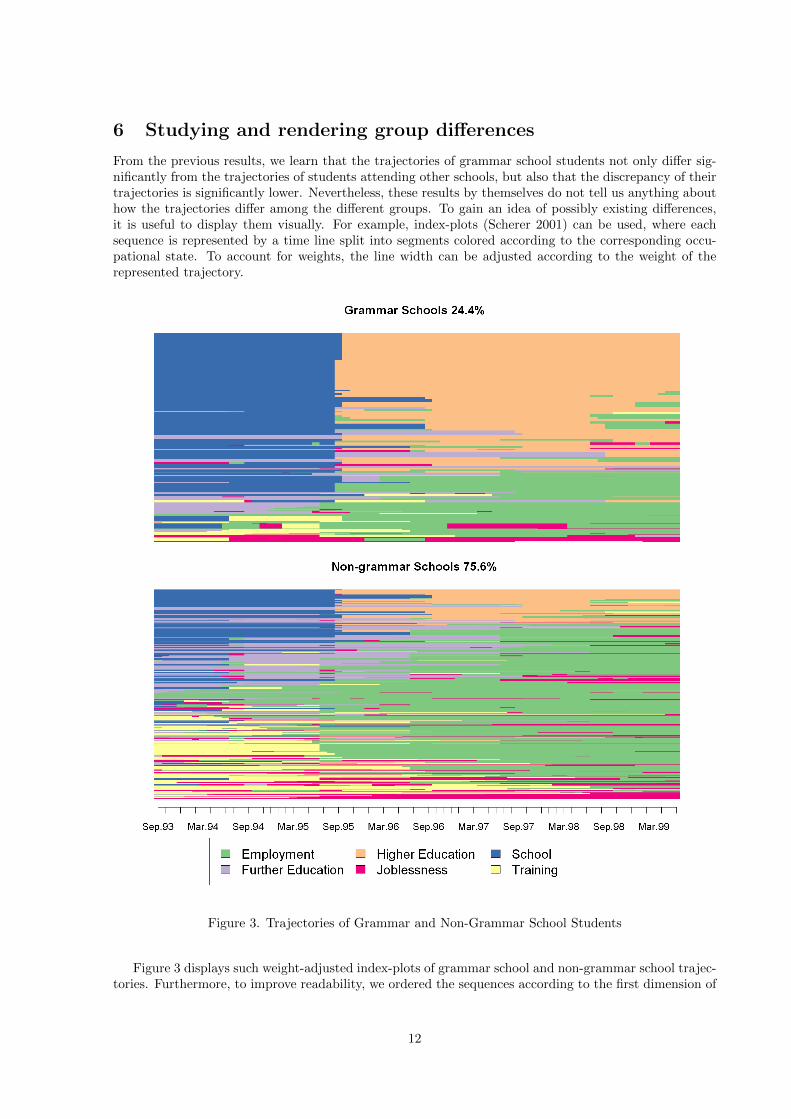
From the previous results, we learn that the trajectories of grammar school students not only differ sig-nificantly from the trajectories of students attending other schools, but also that the discrepancy of theirtrajectories is significantly lower. Nevertheless, these results by themselves do not tell us anything abouthow the trajectories differ among the different groups. To gain an idea of possibly existing differences,it is useful to display them visually. For example, index-plots (Scherer 2001) can be used, where eachsequence is represented by a time line split into segments colored according to the corresponding occu-pational state. To account for weights, the line width can be adjusted according to the weight of therepresented trajectory.

Figure 3. Trajectories of Grammar and Non-Grammar School Students

Figure 3 displays such weight-adjusted index-plots of grammar school and non-grammar school trajec-tories. Furthermore, to improve readability, we ordered the sequences according to the first dimension of

12

a weighted principal coordinate analysis (PCO) (Gower 1966).4 While ordering sequences by a principalcoordinate facilitates the interpretation of the index-plot, the plots provide conversely useful informationfor interpreting the PCO axis. For instance, we observe in our case that the sequences are organized in acontinuum ranging from higher education trajectories to training trajectories, while middle values corre-spond to employment-dominated trajectories. Comparing both populations, it appears that young peoplewho attended grammar schools typically remain in the “school” state and are more likely to proceed tohigher education, while those who attended other types of schools follow more diverse trajectories.

0.05

0.07

0.09

020

4060

8012

0

Pseudo R2

Levene

Sep.93 Apr.94 Nov.94 Jun.95 Jan.96 Aug.96 Apr.97 Nov.97 Jun.98 Jan.99

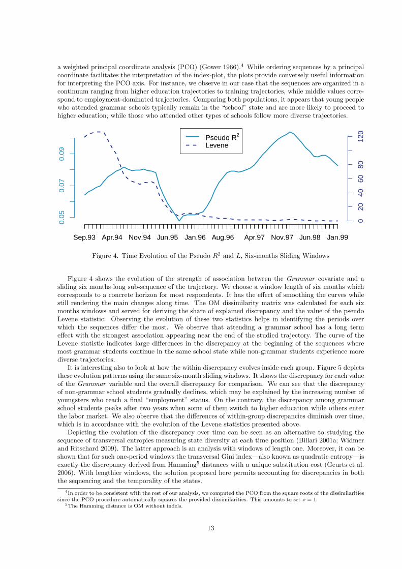
Figure 4. Time Evolution of the Pseudo R2 and L, Six-months Sliding Windows

Figure 4 shows the evolution of the strength of association between the Grammar covariate and asliding six months long sub-sequence of the trajectory. We choose a window length of six months whichcorresponds to a concrete horizon for most respondents. It has the effect of smoothing the curves whilestill rendering the main changes along time. The OM dissimilarity matrix was calculated for each sixmonths windows and served for deriving the share of explained discrepancy and the value of the pseudoLevene statistic. Observing the evolution of these two statistics helps in identifying the periods overwhich the sequences differ the most. We observe that attending a grammar school has a long termeffect with the strongest association appearing near the end of the studied trajectory. The curve of theLevene statistic indicates large differences in the discrepancy at the beginning of the sequences wheremost grammar students continue in the same school state while non-grammar students experience morediverse trajectories.

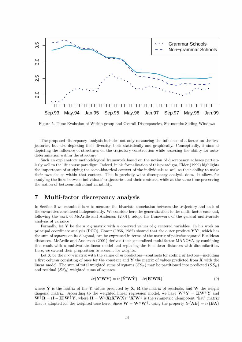
It is interesting also to look at how the within discrepancy evolves inside each group. Figure 5 depictsthese evolution patterns using the same six-month sliding windows. It shows the discrepancy for each valueof the Grammar variable and the overall discrepancy for comparison. We can see that the discrepancyof non-grammar school students gradually declines, which may be explained by the increasing number ofyoungsters who reach a final “employment” status. On the contrary, the discrepancy among grammarschool students peaks after two years when some of them switch to higher education while others enterthe labor market. We also observe that the differences of within-group discrepancies diminish over time,which is in accordance with the evolution of the Levene statistics presented above.

Depicting the evolution of the discrepancy over time can be seen as an alternative to studying thesequence of transversal entropies measuring state diversity at each time position (Billari 2001a; Widmerand Ritschard 2009). The latter approach is an analysis with windows of length one. Moreover, it can beshown that for such one-period windows the transversal Gini index—also known as quadratic entropy—isexactly the discrepancy derived from Hamming5 distances with a unique substitution cost (Geurts et al.2006). With lengthier windows, the solution proposed here permits accounting for discrepancies in boththe sequencing and the temporality of the states.

4In order to be consistent with the rest of our analysis, we computed the PCO from the square roots of the dissimilaritiessince the PCO procedure automatically squares the provided dissimilarities. This amounts to set ν = 1.

5The Hamming distance is OM without indels.

13

2.0

2.5

3.0

3.5 Grammar Schools

Non−grammar Schools

Sep.93 May.94 Jan.95 Sep.95 May.96 Jan.97 Sep.97 May.98 Jan.99

Figure 5. Time Evolution of Within-group and Overall Discrepancies, Six-months Sliding Windows

The proposed discrepancy analysis includes not only measuring the influence of a factor on the tra-jectories, but also depicting their diversity, both statistically and graphically. Conceptually, it aims atdepicting the influence of structures on the trajectory construction while assessing the ability for auto-determination within the structure.

Such an explanatory methodological framework based on the notion of discrepancy adheres particu-larly well to the life course paradigm. Indeed, in his formalization of this paradigm, Elder (1999) highlightsthe importance of studying the socio-historical context of the individuals as well as their ability to maketheir own choice within that context. This is precisely what discrepancy analysis does. It allows forstudying the links between individuals’ trajectories and their contexts, while at the same time preservingthe notion of between-individual variability.

7 Multi-factor discrepancy analysis

In Section 5 we examined how to measure the bivariate association between the trajectory and each ofthe covariates considered independently. We consider here the generalization to the multi-factor case and,following the work of McArdle and Anderson (2001), adopt the framework of the general multivariateanalysis of variance .

Formally, let Y be the n × q matrix with n observed values of q centered variables. In his work onprincipal coordinate analysis (PCO), Gower (1966, 1982) showed that the outer product YY′, which hasthe sum of squares on its diagonal, can be expressed in terms of the matrix of pairwise squared Euclideandistances. McArdle and Anderson (2001) derived their generalized multi-factor MANOVA by combiningthis result with a multivariate linear model and replacing the Euclidean distances with dissimilarities.Here, we extend their proposition to account for weights.

Let X be the n×m matrix with the values of m predictors—contrasts for coding M factors—includinga first column consisting of ones for the constant and Y the matrix of values predicted from X with thelinear model. The sum of total weighted sums of squares (SST ) may be partitioned into predicted (SSB)and residual (SSR) weighted sums of squares.

tr(Y′WY

)= tr

(Y′WY

)+ tr

(R′WR

)(9)

where Y is the matrix of the Y values predicted by X, R the matrix of residuals, and W the weightdiagonal matrix. According to the weighted linear regression model, we have W

12 Y = HW

12 Y and

W12 R = (I−H)W

12 Y, where H = W

12 X(X′WX)−1X′W

12 is the symmetric idempotent “hat” matrix

that is adapted for the weighted case here. Since W = W12 W

12 , using the property tr

(AB

)= tr

(BA

)14

for conformable matrices, Equation (9) may be rewritten as:

tr(WYY′

)= tr

(W

12 HW

12 YY′

)+ tr

[W

12 (I−H)W

12 YY′

](10)

Let us now look at Gower’s result that expresses G = YY′ in terms of the pairwise squared distances.In the formulation retained by McArdle and Anderson (2001), we have G = − 1

2

(I− 1

n11′)D(I− 1

n11′),

where 1 is a vector of ones of length n, I the identity matrix, and D the n × n matrix of the squaredpairwise Euclidean distances. Here, we have to adapt this definition for y variables centered on theirweighted means. In that case, it reads as follows:

G = −1

2

(I− 1

W11′W

)D(I− 1

WW11′

)(11)

The generic element of G is gij = − 12

(d2ij − d2i − d2j + d2

), where d2i , d

2j and d2 are respectively the row

i, the column j, and the overall weighted average of the squared Euclidean distances. It can be shownthat when q = 1, each diagonal element gii of G is the contribution of the i-th individual to the sum ofsquares as defined in Equation (4).6

Setting HW = W12 HW

12 , the total SST , between SSB and within SSW sums of squares of interest

may be rewritten in terms of this adapted G matrix as:

SST = tr(WG

)(12)

SSB = tr(HWG

)(13)

SSW = tr[(W −HW)G

)](14)

The idea is to substitute the pairwise dissimilarities dνij for the squared Euclidean distances thatdefine D in Equation (11). Assuming such a substitution and using formulas (12–14), we can deriveglobal pseudo-R2 and pseudo-F statistics as defined in Equations (6–7). Instead of the number of groups,m should be set here to the number of columns of X (i.e., to the total number of contrast and/or indicatorvariables necessary for coding the M factors).

For M = 1 (i.e., in the case of a single factor), computing the SST and SSW with the formula ( 2 onpage 5) as shown in Section 5 gives exactly the same results as the matrix formulation considered here.However, the direct computation of the sums of squares is about 10 times faster.

We may also consider the contribution of each covariate to the total discrepancy reduction. Aswith multi-factor ANOVA, there are different ways of looking at these individual contributions. Shawand Mitchell-Olds (1993) distinguish, among others, between two methods called Type I and Type II,respectively. The Type I method is incremental, which means that covariates are successively added tothe model and the contribution of each covariate is measured by the SSB increase that results when it isintroduced. With this method, the measured impact of each covariate depends on the order in which thecovariates are introduced. With the Type II method, known to be robust in the absence of interactioneffects, the contribution of each covariate is measured by the reduction of SSB that occurs when we dropit out from the full model (i.e., from the model with all covariates). We retain the second method andhence compute the following F for each covariate v

Fv =(SSBc − SSBv )/p

SSWc/(W −m− 1)

(15)

where the SSBcand SSWc

are the explained and residual sums of squares of the full model, SSBvthe

explained sum of squares of the model after removing variable v, and p the number of indicators orcontrasts used to encode the covariate v.

As in the single discrepancy analysis, the F distribution is not relevant for the pseudo-F , and weconsider again permutation tests for assessing the significance of the F statistic. Since Fv is intended fortesting the conditional independence of v, its null distribution is obtained by permuting only the covariatev while the global F statistic is computed by permuting the whole profiles. Thus, for a complete multi-factor analysis with profiles defined by M factors, 1 + M permutation tests are required, which may bequite time-consuming.

6Though it is not a concern here, this result can easily be extended for q > 1.

15

Table 5. Multi-Factor Discrepancy Analysis

Full Model Backward ModelVariable Fv ∆R2

v Sig Fv ∆R2v Sig

gcse5eq 51.91 0.060 0.000 55.72 0.065 0.000grammar 20.77 0.024 0.000 21.44 0.025 0.000sex 5.47 0.006 0.002 5.30 0.006 0.003funemp 3.59 0.004 0.039 3.83 0.004 0.028fmpr 3.30 0.004 0.054region 3.19 0.015 0.004 3.37 0.016 0.003religion 2.29 0.003 0.212livboth 1.80 0.002 0.405

Ftot R2tot Sig Ftot R2

tot Sig

Global 14.96 0.190 0.000 19.55 0.182 0.000

Let us look at what a multi-factor analysis gives for our illustrative example. Table 5 shows the resultsfor two models: the complete model with all variables and a model obtained after removing non-significantcovariates through a backward stepwise process. The tests were conducted using 5,000 permutations.

Both models provide overall significant information about the discrepancy of the trajectories sinceboth global F statistics are significant. The full model explains a slightly higher part of the discrepancy(R2 = 0.190) than does the backward model (R2 = 0.182), but it contains non-significant covariates.

In the full model, the variable “qualification gained at the end of compulsory education” (gcse5eq)is the most significant covariate. If we remove this variable, the R2 of the model (= 0.190) decreasesby 0.060. The difference is significant since we have Fgcse5eq = 51.91, which was never attained with5,000 permutations. As before, the variable religion is not significant. Removing it from the modelreduces the R2 by only 0.003 and results in a Freligion value of 2.29 and a p-value of 0.208. Likewise,the variable “having a professional, managerial or related father” (fmpr) loses its significance in themulti-factor case. In fact, the variable fmpr becomes non-significant as soon as we control for “father’sunemployment” (funemp), as the two variables are strongly correlated and “father’s unemployment” isthe most significant one.

The multi-factor approach provides information about the proper effect of the covariates on theoccupational trajectory (i.e., about the part of the total effect that is not accounted for by factorsthat are already introduced). In that sense, the multi-factor approach is complementary to the singleunivariate discrepancy analysis which informs on the raw effect of each covariate. Nevertheless, while themulti-factor approach permits us to know which effects are significant, it does not tell us much aboutwhat the effects are (i.e., about how trajectories may change with the value of the covariates). To answersuch questions, we propose a tree approach which can be seen as an extension of the graphical displayshown in Figure 3.

8 Tree-structured analysis of sequences

In this section, we complement the sequence discrepancy analysis with the regression tree method intro-duced in Studer et al. (2009, 2010) which we extend to account for weighted sequences. Regression treeswork as follows (Morgan and Sonquist 1963; Breiman, Friedman, Olshen, and Stone 1984). They startwith all individuals grouped in an initial node. Then, they recursively partition each node using valuesof a predictor. At each node, the predictor and the split are chosen in such a way that the resulting childnodes differ as much as possible from one another or have, more or less equivalently, lowest within-groupdiscrepancy. The process is repeated on each new node until a certain stopping criterion is reached.

The recursive partitioning generated by a tree is known to provide an easily comprehensible viewof how each newly selected covariate nuances the effect of covariates introduced at earlier levels. Thisrequires the display of relevant information about the distribution at each node. We could represent themedoid (i.e., the observed sequence that minimizes the dissimilarity (Equation 4) between the sequenceand the group gravity center). It would be instructive to render the within-group discrepancy as well.Although this is not obvious for any kind of complex objects, displaying index-plots like those used in

16

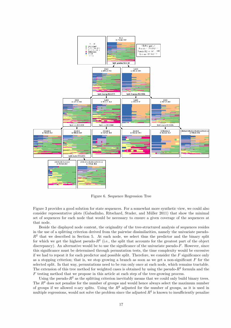
Figure 6. Sequence Regression Tree

Figure 3 provides a good solution for state sequences. For a somewhat more synthetic view, we could alsoconsider representative plots (Gabadinho, Ritschard, Studer, and Muller 2011) that show the minimalset of sequences for each node that would be necessary to ensure a given coverage of the sequences atthat node.

Beside the displayed node content, the originality of the tree-structured analysis of sequences residesin the use of a splitting criterion derived from the pairwise dissimilarities, namely the univariate pseudo-R2 that we described in Section 5. At each node, we select thus the predictor and the binary splitfor which we get the highest pseudo-R2 (i.e., the split that accounts for the greatest part of the objectdiscrepancy). An alternative would be to use the significance of the univariate pseudo-F . However, sincethis significance must be determined through permutation tests, the time complexity would be excessiveif we had to repeat it for each predictor and possible split. Therefore, we consider the F significance onlyas a stopping criterion; that is, we stop growing a branch as soon as we get a non-significant F for theselected split. In that way, permutations need to be run only once at each node, which remains tractable.The extension of this tree method for weighted cases is obtained by using the pseudo-R2 formula and theF testing method that we propose in this article at each step of the tree-growing process.

Using the pseudo-R2 as the splitting criterion inevitably means that we could only build binary trees.The R2 does not penalize for the number of groups and would hence always select the maximum numberof groups if we allowed n-ary splits. Using the R2 adjusted for the number of groups, as it is used inmultiple regressions, would not solve the problem since the adjusted R2 is known to insufficiently penalize

17

complexity. Using information criteria such as the BIC would also not be suitable, as such criteria arehardly derivable in a case where the distribution of the statistics (R2, F or SSW ) under the independencehypothesis is not known.

The global quality of the tree can be assessed through the association strength between the sequencesand the leaf (terminal node) membership. The global pseudo-F provides a way of testing the statisticalsignificance of the obtained segmentation, while the global pseudo-R2 provides a measure of the part ofthe total discrepancy that is explained by the tree.

Figure 6 shows the dissimilarity tree grown using our weighed example dataset. The chosen stoppingcriteria are a p-value of 5% for the F test, a minimal leaf size of 5% of the total sum of weights, and amaximal depth of 5. In each node, we see the plot of the individual sequences as well as the node size,the sum of weights, and the discrepancy s2 within the node. At the bottom of each parent node, weindicate the retained split predictor with the associated R2, while the definition of the binary split maybe inferred from the indication at the top of the child nodes.

The overall R2 of the tree is 0.187, which falls between the global R2 of the full and backward modelsin Table 5. However, the results are now much easier to interpret. Moreover, the tree automaticallyaccounts for interaction effects that were not considered in the multi-factor discrepancy analysis. Weobserve, for instance, that “attending grammar school” discriminates better among students who finishedthe compulsory schooling with high grades than among those who obtained lower grades. Likewise, wecan see that having an unemployed father seems to affect primarily young male Irish with low grades atthe end of compulsory schooling (gcse5eq).

9 Running sequence discrepancy analysis in R with TraMineR

We implemented the methods presented in this article into TraMineR, which is a free package for theR statistical environment (R Development Core Team 2008). Below, we briefly show how to run thediscrepancy analysis features discussed here. We would also like to refer our readers to the TraMineRUser’s guide (Gabadinho, Ritschard, Studer, and Muller 2009), which provides a detailed overview ofother features offered by the package, especially of the rendering of sequences and the computation ofdissimilarities. Our readers can reproduce the results we present here, as the mvad dataset, which weuse, has been made available as part of the TraMineR package, thanks to the authorization of McVicarand Anyadike-Danes.

To begin the analysis, we load the mvad data and create a weighted state sequence object using thecommands below. The state variables from September 1993 to June 1999 are in columns 17 to 86 of thedata frame.7

R> library(TraMineR)

R> data(mvad)

R> mvadseq <- seqdef(mvad[, 17:86], weights = mvad$weight)

Next, we compute the OM dissimilarity matrix with the indel and substitution costs used by McVicarand Anyadike-Danes (2002).

R> subm.custom <- matrix(

+ c(0,1,1,2,1,1,

+ 1,0,1,2,1,2,

+ 1,1,0,3,1,2,

+ 2,2,3,0,3,1,

+ 1,1,1,3,0,2,

+ 1,2,2,1,2,0),

+ nrow = 6, ncol = 6, byrow = TRUE)

R> mvaddist <- seqdist(mvadseq, method = "OM", indel = 1.5, sm = subm.custom)

To perform the univariate discrepancy analysis and to test for homogeneity of discrepancy, we callthe dissassoc() function which takes four arguments: the dissimilarity matrix, the factor (group), thenumber of permutations (R=1000 by default), and an optional weights argument. The results presentedin Section 5 were obtained with the following code:

7For details on TraMineR functions such as seqdef, seqdist, dissassoc presented here see the reference manual ortype for instance ?dissassoc in the R console to access the on-line help.

18

R> dissassoc(mvaddist, group = mvad$gcse5eq, R = 5000,

+ weights = mvad$weight, weight.permutation="diss")

Likewise, we generated Figures 4 and 5 with seqdiff() as shown below.

R> Grammar.diff <- seqdiff(mvadseq, group = mvad$Grammar,

+ seqdist_arg = list(method = "OM", indel = 1.5, sm = subm.custom))

R> plot(Grammar.diff, stat = c("Pseudo R2", "Levene"))

R> plot(Grammar.diff, stat = "discrepancy")

The multi-factor results listed in Table 5 were obtained with the dissmfac() function. The model isspecified as a classical R formula with the dissimilarity matrix on the left-hand side. We use the dataargument to specify the data.frame containing the covariates.8

R> dissmfac(

+ mvaddist ~ gcse5eq + Grammar + funemp + catholic + male + fmpr + livboth + region,

+ data = mvad, R = 5000, weights = mvad$weight)

To carry out a tree-structured analysis of the sequences, we use the seqtree() function. The dissim-ilarity matrix and the predictors are passed to the function in the same way as in dissmfac(). Stoppingcriteria can be set with the arguments minSize for the minimum node size, maxdepth for the maximumtree depth and pval for the minimum required p-value. As for dissassoc(), the R argument controlsthe number of permutations for computing the p-values. Notice that it is not necessary to specify theweights since they are already attached to the state sequence mvadseq object.

R> mvadtree <- seqtree(

+ mvadseq ~ gcse5eq + Grammar + funemp + catholic + male + fmpr + livboth + region,

+ data = mvad, minSize = 30, maxdepth = 5, R = 5000, pval = 0.01, diss = mvaddist)

R> print(mvadtree)

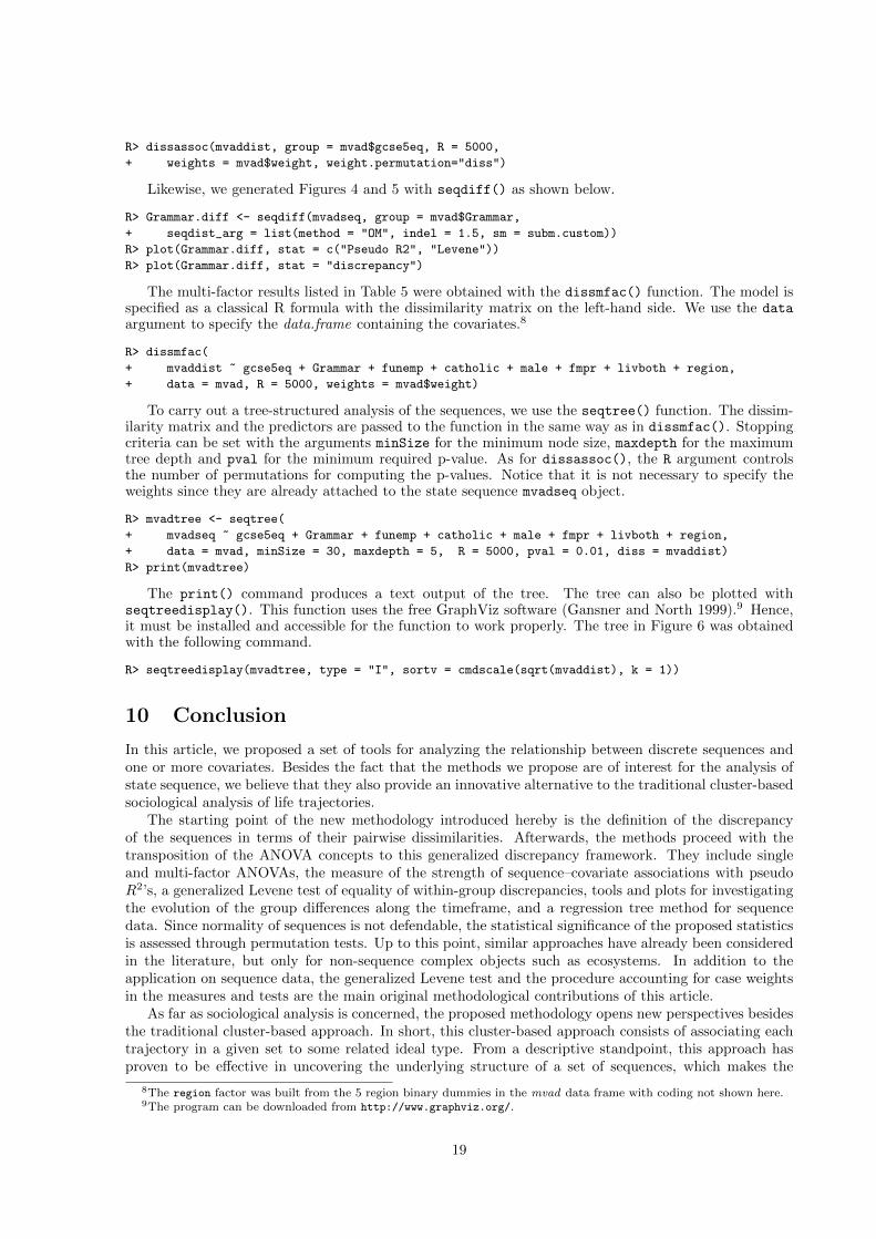
The print() command produces a text output of the tree. The tree can also be plotted withseqtreedisplay(). This function uses the free GraphViz software (Gansner and North 1999).9 Hence,it must be installed and accessible for the function to work properly. The tree in Figure 6 was obtainedwith the following command.

R> seqtreedisplay(mvadtree, type = "I", sortv = cmdscale(sqrt(mvaddist), k = 1))

10 Conclusion

In this article, we proposed a set of tools for analyzing the relationship between discrete sequences andone or more covariates. Besides the fact that the methods we propose are of interest for the analysis ofstate sequence, we believe that they also provide an innovative alternative to the traditional cluster-basedsociological analysis of life trajectories.

The starting point of the new methodology introduced hereby is the definition of the discrepancyof the sequences in terms of their pairwise dissimilarities. Afterwards, the methods proceed with thetransposition of the ANOVA concepts to this generalized discrepancy framework. They include singleand multi-factor ANOVAs, the measure of the strength of sequence–covariate associations with pseudoR2’s, a generalized Levene test of equality of within-group discrepancies, tools and plots for investigatingthe evolution of the group differences along the timeframe, and a regression tree method for sequencedata. Since normality of sequences is not defendable, the statistical significance of the proposed statisticsis assessed through permutation tests. Up to this point, similar approaches have already been consideredin the literature, but only for non-sequence complex objects such as ecosystems. In addition to theapplication on sequence data, the generalized Levene test and the procedure accounting for case weightsin the measures and tests are the main original methodological contributions of this article.

As far as sociological analysis is concerned, the proposed methodology opens new perspectives besidesthe traditional cluster-based approach. In short, this cluster-based approach consists of associating eachtrajectory in a given set to some related ideal type. From a descriptive standpoint, this approach hasproven to be effective in uncovering the underlying structure of a set of sequences, which makes the

8The region factor was built from the 5 region binary dummies in the mvad data frame with coding not shown here.9The program can be downloaded from http://www.graphviz.org/.

19

data easier to understand. However, relying on clusters for studying the relationship between sequencesand their context can be criticized on the basis that reducing the set of sequences to a limited numberof standard trajectories is a rather crude approximation and would lead to considering deviations fromthe standard inside a cluster as non-explained error terms. As a result of this approximation, wrongconclusions may be drawn about relationships between the sequences and their context. On the otherhand, the approach we propose here takes into account explicitly how the individual characteristics affectthe trajectory followed by each individual.

Furthermore, in this paper we adopted an explanatory methodological framework that complies withthe life course paradigm (Elder 1999) by accounting for the individuals’ ability to make their own choiceswithin their socio-historical backgrounds when estimating the sequence–context relationship. By focusingon the discrepancy of the sequences, they allow studying the link between the trajectories and their contextwhile preserving the notion of between-individual variability.

The choice of the measure of dissimilarity between sequences is a recurrent debate in the socialsciences (Dijkstra and Taris 1995; Wu 2000; Elzinga 2003), which is beyond the scope of the presentpaper. Although we have illustrated the methods using an optimal matching edit distance, the methodsconsidered in this paper are by no way limited to optimal matching. They work with any dissimilaritymeasure. Moreover, running the statistical tests with different dissimilarity measures provides a wayof assessing their respective discriminant power for the data at hand. Also, using, for instance, themultichannel approach considered by Pollock (2007), the proposed methods could be applied on parallelsequences such as those describing, for example, linked lives or joint occupational and cohabitationaltrajectories. The observed differences between groups could then result from any of the channel, orfrom the combination of channels.10 Even more generally, the discrepancy analysis is not limited tosequence data. If we except the graphical rendering of the results, they apply to any objects that can becharacterized by a pairwise dissimilarity matrix.

Finally, we would like to remind our readers that all the proposed tools have been implemented inthe TraMineR library for the R statistical environment. They are thus readily and freely accessible toany interested reader as illustrated in Section 9.

Acknowledgments:

We gratefully thank Nevena Zhelyazkova for her careful reading of the manuscript and the anonymousreviewers for their constructive comments and suggestions.

Funding

This research was supported by the Swiss National Science Foundation (Grant SNSF 100015-122230).

A Proofs

In this appendix, we present the mathematical developments underlying the results presented in thearticle. The presentation is largely inspired from Spath (1975) and Batagelj (1988).

We begin with a proof of Equation (1) that expresses the sum of squares in terms of pairwise Euclideandistances. Here we demonstrate it for the more general multivariate case. Let yi be the data vector forcase i, wi its associated weight, W =

∑ni=1 wi the sum of the weights, and y = 1

W

∑ni=1 wiyi the vector

of weighted averages. Letting ‖y‖2 denote the squared length of the vector, that is y′y =∑i y

2i , the

multivariate result that we want to establish is:

Theorem 1 Sum of squares in terms of pairwise distances

SS =

n∑i=1

wi‖yi − y‖2 =1

W

n∑i=1

n∑j=i+1

wiwj‖yi − yj‖2 (16)

10It should be noted, however, that such a multichannel analysis is not intended for studying the link between the channels.

20

Proof. We first show that the sum of squared distances to a point x is

n∑i=1

wi‖yi − x‖2 =

n∑i=1

wi‖yi − y‖2 +W‖y − x‖2 (17)

Since yi − x = (yi − y) + (y − x), its squared length is

‖yi − x‖2 = ‖yi − y‖2 + 2(y − x)′(yi − y) + ‖y − x‖2

Weighting with wi and summing over i, we get

n∑i=1

wi‖yi − x‖2 = 2(y − x)′n∑i=1

wi(yi − y) +

n∑i=1

wi‖yi − y‖2 +W‖y − x‖2 (18)

Since,∑ni=1 wi(yi− y) = 0, the middle term on the right-hand side vanishes, which yields Equation (17).

Setting x = yj , multiplying by wj and summing over j results in

n∑j=1

n∑i=1

wiwj‖yi − yj‖2 =

n∑j=1

wj

n∑i=1

wi‖yi − y‖2 +W

n∑j=1

wj‖y − yj‖2

= 2W

n∑i=1

wi‖yi − y‖2 (19)

The left-hand side can be written as 2∑ni=1

∑nj=i+1 wiwj‖yi − yj‖2. Then, dividing both sides by 2W

we get Equation 16 of Theorem 1. �

Theorem 2 Contribution to the sum of squares. It can be expressed as follows in terms of pairwisedistances.

‖y − x‖2 =1

W

( n∑i=1

wi‖x− yi‖2 − SS)

(20)

Proof. Extracting ‖x− y‖2 from Equation (17), we get

‖y − x‖2 =1

W

( n∑i=1

wi‖yi − x‖2 −n∑i=1

wi‖yi − y‖2)

(21)

The second term in the parenthesis is just SS, which proves the Theorem. �

Replacing x with yj , we can see that ‖y − yj‖2 is the contribution of yj to SS by multiplyingEquation (20) by wj and summing over j. As a result, we obtain

∑j wj‖y − yj‖2 = 2SS − SS = SS,

hence the sum of squares. What makes the formula interesting is that it expresses the contribution interms of pairwise distances. Formula ( 4 on page 5) is just Theorem 2 with dissimilarities dν substitutedin place of the squared Euclidean distances ‖.‖2.

We now prove the following result about the non-negativity of the contribution.

Theorem 3 Non-negativity of the contribution to the sum of squares (sufficient condition).Let d be a dissimilarity measure and assume the generalized sum of squares SS is calculated with dν .Then, the contribution of x to the sum of squares SS

dνxg =1

W

( n∑i=1

widνxi − SS

)(22)

is non-negative when dν respects the triangle inequality.

21

Proof. Replacing SS by its expression in terms of pairwise dissimilarities (Theorem 1), the contribution(i.e., Equation (22)), can be re-written as

dνxg =1

2W 2

n∑i=1

n∑j=1

wiwj(2dνix − dνij

)(23)

In this form, it appears that the smallest value of the contribution dνxg is obtained when all dνij ’s taketheir maximal possible value. Under the triangle inequality, dνij cannot exceed dνxi + dνxj . Hence, dνxgreaches its minimum when dνij = dνxi + dνxj for all i and j. This minimum is zero, which implies dνxg ≥ 0.�

B Should dissimilarities be squared?

In this appendix, we discuss the choice of the ν exponent in Equation (2). Should we square the dis-similarities when computing the generalized sum of squares, or is it preferable to substitute the squaredEuclidean distances with the dissimilarities themselves?

If the chosen dissimilarity between sequences can be represented univocally as a distance in an as-sociated Euclidean coordinate space, we would have to set ν = 2 to get a generalized SS equal tothe corresponding sum of squares in that space (Gower 1982). While dissimilarities between strings ofcharacters that can be expressed as kernels (Lodhi, Saunders, Shawe-Taylor, Cristianini, and Watkins2002) have this property, most cost-minimizing distances such as OM cannot be expressed as Euclideandistances.

There are several arguments in favor of setting ν = 1. According to Mielke and Berry (1983), thissolution leads to a strongest congruence between analysis and data space. Moreover, it should producemore robust results when the corresponding points in the coordinate space are not normally distributed.From our point of view, the strongest argument to set ν = 1 is related to the triangle inequality. Indeed,when the dissimilarity d respects the triangle inequality,

√d respects it too, while generally d2 does not.

Since the triangle inequality of dν ensures that SS cannot be greater than the sum of distances∑i wid

νxi

to any arbitrary chosen object x, we would then be sure that SS does not exceed the sum∑i wid

νxi with

ν = 1, while it would not be the case with ν = 2. The same argument can be formalized differently in termsof the contribution (4) to the sum of squares SS. The non-negativity of this contribution automaticallyresults when dνij satisfies the triangle inequality (see Appendix A), while negative contributions to thediscrepancy can occur when the triangle inequality does not hold. Hence, ν = 1 ensures non-negativecontributions when d satisfies the triangle inequality.

A negative value of the dissimilarity dνxg between x and the center of gravity g means that accountingfor the object x reduces the sum of squares. This can be the case when two objects, say y and z, becomecloser when we can pass through x (i.e., when dyz > dyx + dxz). Such situations are common in socialnetwork analysis. Consider, for instance, a network between x, y and z where the dissimilarity is equalto 1 for two people that meet often and is equal to 10 when they never meet. The dissimilarity dxgwould then be negative if x often meets both y and z while y never meets z. From a social networkperspective, we would say that x plays a cohesive role in the network. Although a negative contributionto the discrepancy is relevant in such settings, it is most often not the case. Hence, the results should beinterpreted with caution when dνij does not respect the triangle inequality, which may occur with ν = 2as noted above. In particular, in such situations one should be ready to accept and give meaning tonegative contributions to the discrepancy.

To summarize, we suggest defining SS with ν = 1, except when we can express the dissimilaritymeasure as an Euclidean distance, in which case ν = 2 is best suited.

C About the number of permutations in permutation tests

It is generally admitted that 1,000 permutations are sufficient to assess a result at the 5% level, while5,000 are necessary at the 1% level. Here, we present some figures to support this claim.

Let p be the true p-value of Fobs and p be the proportion of F ’s smaller than Fobs among R random-izations. Table 6 shows how the probability P (p < 1.2p | p) that the empirical p-value does not exceed

22

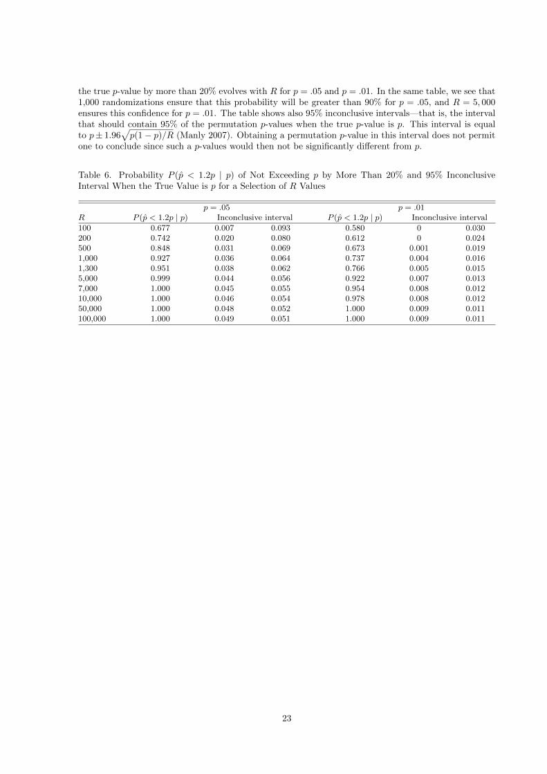
the true p-value by more than 20% evolves with R for p = .05 and p = .01. In the same table, we see that1,000 randomizations ensure that this probability will be greater than 90% for p = .05, and R = 5, 000ensures this confidence for p = .01. The table shows also 95% inconclusive intervals—that is, the intervalthat should contain 95% of the permutation p-values when the true p-value is p. This interval is equalto p± 1.96

√p(1− p)/R (Manly 2007). Obtaining a permutation p-value in this interval does not permit

one to conclude since such a p-values would then not be significantly different from p.

Table 6. Probability P (p < 1.2p | p) of Not Exceeding p by More Than 20% and 95% InconclusiveInterval When the True Value is p for a Selection of R Values

p = .05 p = .01R P (p < 1.2p | p) Inconclusive interval P (p < 1.2p | p) Inconclusive interval

100 0.677 0.007 0.093 0.580 0 0.030200 0.742 0.020 0.080 0.612 0 0.024500 0.848 0.031 0.069 0.673 0.001 0.0191,000 0.927 0.036 0.064 0.737 0.004 0.0161,300 0.951 0.038 0.062 0.766 0.005 0.0155,000 0.999 0.044 0.056 0.922 0.007 0.0137,000 1.000 0.045 0.055 0.954 0.008 0.01210,000 1.000 0.046 0.054 0.978 0.008 0.01250,000 1.000 0.048 0.052 1.000 0.009 0.011100,000 1.000 0.049 0.051 1.000 0.009 0.011

23

References

Abbott, Andrew. 1990. “A Primer on Sequence Methods.” Organization Science 1:375–392.

Abbott, Andrew and John Forrest. 1986. “Optimal Matching Methods for Historical Sequences.” Journalof Interdisciplinary History 16:471–494.

Abbott, Andrew and Alexandra Hrycak. 1990. “Measuring Resemblance in Sequence Data: An OptimalMatching Analaysis of Musician’s Carrers.” American Journal of Sociolgy 96:144–185.

Anderson, Marti Jane. 2001. “A new method for non-parametric multivariate analysis of variance.”Austral Ecology 26:32–46.

. 2006. “Distance-Based Tests for Homogeneity of Multivariate Dispersions.” Biometrics 62:245–253.

Bartlett, Maurice Stevenson. 1937. “Properties of Sufficiency and Statistical Tests.” Proceedings of theRoyal Society of London. Series A, Mathematical and Physical Sciences 160:268–282.

Batagelj, Vladimir. 1988. “Generalized Ward and related clustering problems.” In Classification andrelated methods of data analysis, edited by Hans H. Bock, pp. 67–74. Amsterdam: North-Holland.

Billari, Francesco Candeloro. 2001a. “The Analysis of Early Life Courses: Complex Description of theTransition to Adulthood.” Journal of Population Research 18:119–142.

. 2001b. “A Log-Logistic Regression Model for a Transition Rate with a Starting Threshold.”Population Studies 55:15–24.

. 2005. “Life Course Analysis: Two (Complementary) Cultures? Some Reflections With Ex-amples From The Analysis Of Transition To Adulthood.” In Towards an Interdisciplinary Perspectiveon the Life Course, edited by Rene Levy, Paolo Ghisletta, Jean-Marie Le Goff, Dario Spini, and EricWidmer, Advances in Life Course Research, Vol. 10, pp. 267–288. Amsterdam: Elsevier.

Blossfeld, Hans-Peter and Gotz Rohwer. 2002. Techniques of Event History Modeling, New Approachesto Causal Analysis. Mahwah NJ: Lawrence Erlbaum, 2nd edition.

Breiman, Leo, Jerome H. Friedman, R. A. Olshen, and C. J. Stone. 1984. Classification And RegressionTrees. New York: Chapman and Hall.

Brown, Morton B. and Alan B. Forsythe. 1974a. “Robust Tests for the Equality of Variances.” Journalof the American Statistical Association 69:364–367.

. 1974b. “The Small Sample Behavior of Some Statistics Which Test the Equality of SeveralMeans.” Technometrics 16:129–132.

Cuadras, Carles M. 2008. “Distance-Based Association and Multi-Sample Tests for General MultivariateData.” In Advances in Mathematical and Statistical Modeling , edited by Barry C. Arnold, N. Balakr-ishnan, Jose-Maria Sarabia, and Roberto Minguez, Statistics for Industry and Technology. BirkhauserBoston.

Delicado, Pedro. 2007. “Functional k-sample problem when data are density functions.” ComputationalStatistics 22:391–410.

Dijkstra, Will and Toon Taris. 1995. “Measuring the Agreement between Sequences.” Sociological Methodsand Research 24:214–231.

Elder, Glen H. 1999. Children of the Great Depression. Westview Press.

Elzinga, Cees H. 2003. “Sequence Similarity: A Non-Aligning Technique.” Sociological Methods andResearch 31:214–231.

. 2007. “Sequence Analysis: Metric Representations of Categorical Time Series.” Manuscript,Dept of Social Science Research Methods, Vrije Universiteit, Amsterdam.

. 2010. “Complexity of categorical time series.” Sociological Methods and Research 38:463–481.

Elzinga, Cees H. and Aart C. Liefbroer. 2007. “De-standardization of Family-Life Trajectories of YoungAdults: A Cross-National Comparison Using Sequence Analysis.” European Journal of Population23:225–250.

Gabadinho, Alexis, Gilbert Ritschard, Matthias Studer, and Nicolas S. Muller. 2009. “Mining SequenceData in R with the TraMineR package: A User’s Guide.” Technical report, Department of Econometricsand Laboratory of Demography, University of Geneva, Geneva.

. 2010. “Indice de complexite pour le tri et la comparaison de sequences categorielles.” Revuedes nouvelles technologies de l’information RNTI E-19:61–66.

24

. 2011. “Extracting and Rendering Representative Sequences.” In Knowledge Discovery, Knowl-edge Engineering and Knowledge Management , edited by Ana Fred, Jan L. G. Dietz, Kecheng Liu, andJoaquim Filipe, volume 128 of Communications in Computer and Information Science (CCIS), pp.94–106. Springer-Verlag.

Gansner, Emden R. and Stephen C. North. 1999. “An Open Graph Visualization System and Its Appli-cations to software engineering.” Software - Practice and Experience 30:1203–1233.

Geurts, Pierre, Louis Wehenkel, and Florence d’Alche Buc. 2006. “Kernelizing the output of tree-basedmethods.” In ICML, edited by William W. Cohen and Andrew Moore, volume 148 of ACM Interna-tional Conference Proceeding Series, pp. 345–352. ACM.

Gower, John Clifford. 1966. “Some Distance Properties of Latent Root and Vector Methods Used inMultivariate Analysis.” Biometrika 53:325–338.

. 1982. “Euclidean Distance Geometry.” Mathematical Scientist 7:1–14.

Gower, John Clifford and Wojtek J. Krzanowski. 1999. “Analysis of distance for structured multivariatedata and extensions to multivariate analysis of variance.” Journal of the Royal Statistical Society:Series C (Applied Statistics) 48:505–519.

Jobson, J. D. 1991. Applied Multivariate Data Analysis, volume I: Regression and Experimental design.New York: Springer-Verlag.

Lesnard, Laurent. 2010. “Setting Cost in Optimal Matching to Uncover Contemporaneous Socio-TemporalPatterns.” Sociological Methods and Research 38:389–419.

Lodhi, Huma, Craig Saunders, John Shawe-Taylor, Nello Cristianini, and Chris Watkins. 2002. “Textclassification using string kernels.” The Journal of Machine Learning Research 2:419–444.

Manly, Bryan F. J. 2007. Randomization, Bootstrap and Monte Carlo Methods in Biology . Chapman &Hall, third edition edition.

McArdle, Brian H. and Marti J. Anderson. 2001. “Fitting Multivariate Models to Community Data: AComment on Distance-Based Redundancy Analysis.” Ecology 82:290–297.

McVicar, Duncan and Michael Anyadike-Danes. 2002. “Predicting successful and unsuccessful transitionsfrom school to work using sequence methods.” Journal of the Royal Statistical Society A 165:317–334.

Mielke, Paul W. and Kenneth J. Berry. 1983. “Asymptotic clarifications, generalizations, and concernsregarding an extended class of matched pairs tests based on powers of ranks.” Psychometrika 48:483–485.

. 2007. Permutation Methods: A Distance Function Approach. New York: Springer, 2nd editionedition.

Morgan, J. N. and J. A. Sonquist. 1963. “Problems in the Analysis of Survey Data, and a Proposal.”Journal of the American Statistical Association 58:415–434.

Piccarreta, Raffaella. 2010. “Binary trees for dissimilarity data.” Computational Statistics and DataAnalysis 54:1516–1524.

Piccarreta, Raffaella and Francesco Candeloro Billari. 2007. “Clustering work and family trajectories byusing a divisive algorithm.” Journal of the Royal Statistical Society A 170:1061–1078.

Pollock, Gary. 2007. “Holistic trajectories: A study of combined employment, housing and family careersby using multiple-sequence analysis.” Journal of the Royal Statistical Society A 170:167–183.

R Development Core Team. 2008. R: A Language and Environment for Statistical Computing . R Foun-dation for Statistical Computing, Vienna, Austria. ISBN 3-900051-07-0.

Reiss, Philip T, M. Henry H Stevens, Zarrar Shehzad, Eva Petkova, and Michael P Milham. 2009. “OnDistance-Based Permutation Tests for Between-Group Comparisons.” Biometrics 66:636–43.

Scherer, Stefani. 2001. “Early Career Patterns: A Comparison of Great Britain and West Germany.”European Sociological Review 17:119–144.

Shaw, Ruth G. and Thomas Mitchell-Olds. 1993. “Anova for Unbalanced Data: An Overview.” Ecology74:1638–1645.

Spath, Helmuth. 1975. Cluster analyse algorithmen. Munchen: R. Oldenbourg Verlag.

Studer, Matthias, Gilbert Ritschard, Alexis Gabadinho, and Nicolas S. Muller. 2009. “Analyse de dis-similarites par arbre d’induction.” Revue des nouvelles technologies de l’information RNTI E-15:7–18.

. 2010. “Discrepancy analysis of complex objects using dissimilarities.” In Advances in Knowl-

25

edge Discovery and Management , edited by Fabrice Guillet, Gilbert Ritschard, Djamel A. Zighed, andHenri Briand, volume 292 of Studies in Computational Intelligence, pp. 3–19. Berlin: Springer.

Widmer, Eric and Gilbert Ritschard. 2009. “The De-Standardization of the Life Course: Are Men andWomen Equal?” Advances in Life Course Research 14:28–39.

Wu, Lawrence L. 2000. “Some Comments on ‘Sequence Analysis and Optimal Matching Methods inSociology: Review and Prospect’.” Sociological Methods Research 29:41–64.

Yujian, Li and Liu Bo. 2007. “A Normalized Levenshtein Distance Metric.” IEEE Transactions OnPattern Analysis And Machine Intelligence 29:1091–1095.

Zapala, Matthew A. and Nicholas J. Schork. 2006. “Multivariate regression analysis of distance matricesfor testing associations between gene expression patterns and related variables.” Proceedings of theNational Academy of Sciences of the United States of America 103:19430–19435.

Matthias Studer is a PhD student in Socioeconomics and a research assistant at the Institute for De-mographic and Life Course Studies at the University of Geneva. He holds a Master degree in economicsand a Master of Advanced Studies in sociology. He is currently working on gender and social inequali-ties at the beginning of academic careers in Switzerland. His research interests include data mining oflongitudinal data such as state and event sequences, dissimilarity analysis and survival trees.

Gilbert Ritschard is a full professor of statistics for the social sciences at the University of Geneva.His current research interests are in life course analysis and the application of exploratory data min-ing methods in social sciences. Beside many contributions to chapter books, He published recently inAdvanced Life Course Research, Studies in Family Planning and in the International Journal of DataMining, Modelling and Management, and co-edited a book on Advances in Knowledge Discovery andManagement. He leads currently a Swiss NSF research project on methods for mining event histories.

Alexis Gabadinho is a scientific collaborator at the Institute for Demographic and Life Course Studiesat the University of Geneva. He holds a post-graduate diploma in demography. His current researchinterests are the application of data mining methods in social sciences and the development of methodsfor categorical state sequences analysis, in particular measures of sequence complexity and methods forsummarizing sets of sequences.

Nicolas S. Muller is currently a PhD student in Sociology and a research assistant at the Institute forDemographic and Life Course Studies at the University of Geneva. He holds a MA in sociology and aMSc in Information Systems. His PhD subject is about the links between life trajectories, socio-economicfactors and health outcomes. He is interested in the application of data mining methods in social sciences,and especially sequence mining and association rules methods.

The authors are the developers of the TraMineR toolbox for analyzing sequence data in R.

26