DISCLAIMER OF QUALITY
58
Room 14-0551 77 Massachusetts Avenue Cambridge, MA 02139 MITLibraries Ph: 617.253.5668 Fax: 617.253.1690 Document Services Email: [email protected] http: //libraries. mit. edu/docs DISCLAIMER OF QUALITY Due to the condition of the original material, there are unavoidable flaws in this reproduction. We have made every effort possible to provide you with the best copy available. If you are dissatisfied with this product and find it unusable, please contact Document Services as soon as possible. Thank you. Due to the poor quality of the original document, there is some spotting or background shading in this document.
Transcript of DISCLAIMER OF QUALITY

Room 14-055177 Massachusetts AvenueCambridge, MA 02139MITLibraries Ph: 617.253.5668 Fax: 617.253.1690
Document Services Email: [email protected]: //libraries. mit. edu/docs
DISCLAIMER OF QUALITYDue to the condition of the original material, there are unavoidableflaws in this reproduction. We have made every effort possible toprovide you with the best copy available. If you are dissatisfied withthis product and find it unusable, please contact Document Services assoon as possible.
Thank you.
Due to the poor quality of the original document, there issome spotting or background shading in this document.

December, 1983 LIDS -P -1 30 9
Revised January, 1985, November, 1985, and July, 1986
An Efficient Decomposition Method
for the Approximate Evaluation
of Tandem Queues with Finite Storage Space
and Blocking
by
Stanley B. Gershwin
35-433
Laboratory for Information and Decision Systems
Massachusetts Institute of Technology
77 Massachusetts AvenueCambridge, Massachusetts 02139
Keywords: 343 inventory levels and throughput in transfer
lines, 570 Markov chain model of transfer lines, 721 reliability
and storage, 683 decomposition approximation of queuing networks
To appear, Operations Research

GERSHWIN, Tandem Queue Decomposition 2
ABSTRACTThis paper presents an efficient method for the evaluation of
performance measures for a class of tandem queuing systems with
finite buffers in which blocking and starvation are important
phenomena. These systems are difficult to evaluate because of
their large state spaces and because they may not be decomposed
exactly. The approximate decomposition approach described here
is based on system characteristics such as conservation of flow.
Comparisons with exact and simulation results indicate that it is
very accurate.
ACKNOWLEDGMENTSThis research has been supported by the U. S. Army Human Enginee-
ring Laboratory under contract DAAK1 l-82-K-0018. I am grateful
for the support and encouragement of Dr. Benjamin E. Cummings and
Mr. Charles Shoemaker. I am also grateful for the suggestions
and comments of Ms. Ellen L. Hahne, Professor Rajan Suri, Profes-
sor Loren K. Platzman, Dr. Daniel Heyman, and a reviewer.
GERSHWIN, Tandem Queue Decomposition 3
This paper presents a method for the analysis (i.e., the cal-
culation of throughput and average buffer levels] of a class of
tandem queuing systems with finite buffers. Such systems are
difficult to treat because of their large state spaces and their
indecomposability. The method is based an a model which approxi-
mates a [k-l)-buffer system by k-l single buffer systems. The
parameters of the single-buffer systems are determined by rela-
tionships ...among_ .the flows through -the_ buffers of the original
system. A simple algorithm is developed to calculate the parame-
ters. Numerical and simulation experience indicate that the
method determines thoughput and average buffer levels accurately.
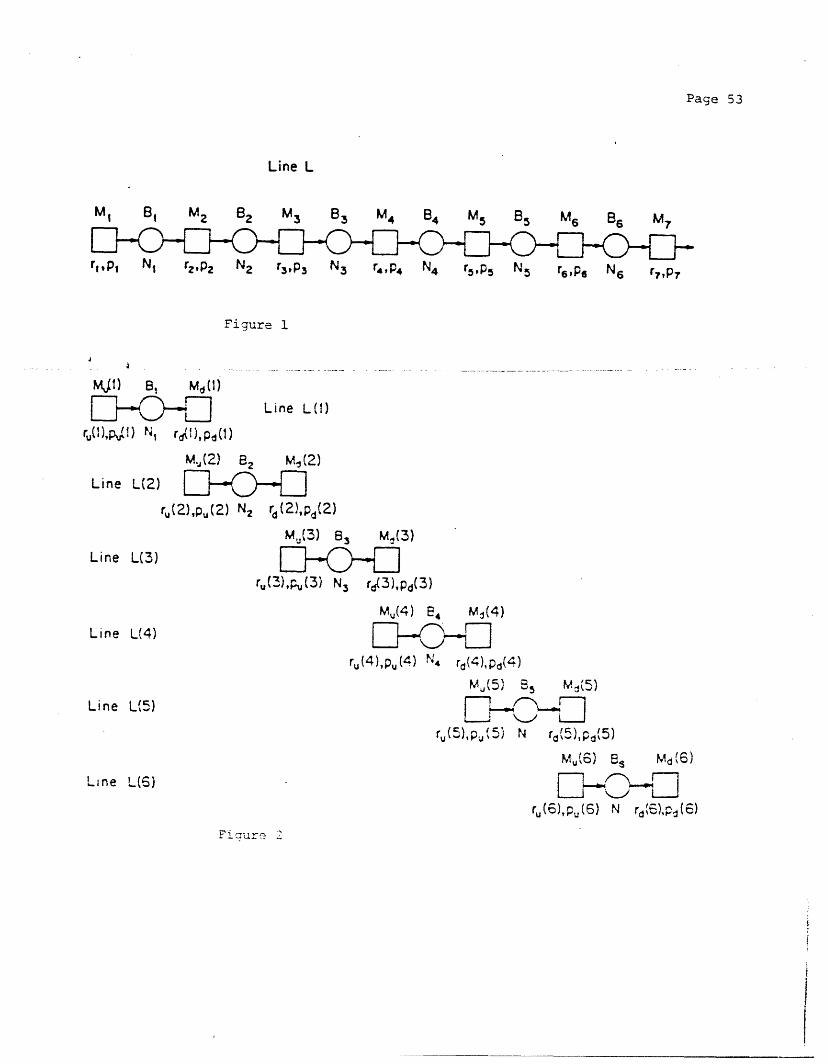
The tandem queuing system in Figure I consists of a series
of k servers or machines [M1, M2, ... , Mk) separated by
buffers (B 1, B2, ... , B_, 1 of finite capacity. Mate-
rial flows from outside the system to M1, then to B1, then to
M2, and so forth until it reaches Mk,, after which it leaves.
In general, in systems of this type, the machines are as-
sumed to spend a random amount of time processing each item. In
this paper, the randomness is due to the failures and repairs of
machines. When machine Mi is down, buffer B1 _ tends to
accumulate material and buffer B1 tends to lose material. If
this condition persists, Bi l may become full or Bi may
become empty. In that case, machine Mil is blocked and
prevented from working or Mi., is starved and also pre-
vented from working.
While a machine is working (i. e., operational and

GERSHWIN, Tandem Queue Decomposition 4
neither starved nor blocked), a fixed amount of time is required
to process a part. This time is the same for all machines and is
taken as the time unit. During a time unit when machine Mi is
working, it has probability Pi of failing. Its mean time
between failures (MTBF] in working time is thus 1/p i. After a
machine has failed, it is under repair and it has probability
ri of being repaired during a time unit. Its mean time to
rep-ai-r-..(MTTR) is therefore 1/r,. -- This '----.is-- measured in clock
time, however, not in working time.
The problem is difficult because of the great size of the
state space. Each machine can be in two states: operational or
under repair. Buffer Bi can be in Ni+ 1 states: n,=0, 1, ....
Ni, where ni is the amount of material in Bi and Ni is
its capacity. As a consequence, the Markov chain representation
of a k-machine line with k-l buffers has a state space of cardi-
nality
k-
2 ' ll[Ni+]J.i=O
A 20-machine line with 19 buffers each of capacity 10, for exam-
ple, has over 6.41 x 1025 states.
Decomposition
We approximate the single k-machine line of Figure 1 by a
set of k-l two-machine lines L(i), i = 1, ... , k-I [Figure 2).
The buffer in L[i] has the same capacity as buffer Bi of the k-
machine line. Both the upstream (Mdfi)) and downstream ([Md(i)l ma-
GERSHWIN, Tandem Queue Decomposition 5
chine in each of the lines are assumed to have a geometric work-
ing time distribution, described by parameters pu(i) and pd([i],
respectively. Their repair times are assumed to be geometrically
distributed with parameters ru(i) and rd(i), respectively. The
four, parameters are chosen (by the algorithm developed in Section
2] so that the performance of machine Mu(i) [[Md[i)) closely matches
that of the line upstream [downstream) of buffer Bi.
That is, the rate of flow into and out of buffer Bi in
line L[i) approximates that of buffer Bi in line L. The proba-
bility of the buffer of line L(i) being empty or full is close to
that of Bi in L being empty or full. The probability of re-
sumption of flow into (and out of) the buffer in line LUi) in a
time unit after a period during which it was interrupted is close
to the probability of the corresponding event in L. Finally, the
average amount of material in the buffer of line L(i) approxi-
mates the material level in buffer Bi in L. In order to find
such parameter values, we use relationships among parameters and
measures of a transfer line.
Machine Mu(i) models the part of the line upstream of B1
and Md(i) models the part of line downstream from Bi. There
are four parameters per two-machine line (i. e., per buffer
in L): ru(i), pu(i), rd(i, pd(i). The decomposition method requires the
determination of four parameters per two-machine line, or a total
of 4(k-1) parameters. To this end, a system of 4(k-1) polynom-
ial equations is derived in Section 2.

GERSHWIN, Tandem Queue Decomposition 6
Literature ; Survey
The Gershwin-Schick (1983) model is based on the transfer
line model of Buzacott (1967). Simulation results for models of
this type appear in Ho et al. (1979), Law (1981), and
Vanderhenst et al. [1981). In the last paper, the authors
refer to historical data that justifies the assumption of expo-
nentially distributed times between failures and until repairs,
although Hanifin, Buzacott and - Taraman, in a simulation paper
[1975), disagree.
Gershwin and Schick (1983) derive an exact solution for
three-machine versions of this system. However, it is difficult
to program, ill-behaved, and is not extendable to larger prob-
lems. Coillard and Proth (1983) describe a method for a related
three-machine model, but again their method does not appear to be
useful for longer lines. Ohmi (1981) provides an approximate me-
thod for larger systems, but he makes certain restrictive as-
sumptions, such as that no more than one machine is down at any
time.
The concept of approximate decomposition of tandem queuing
models was discussed by Hunt (1956), Hillier and Boling (1966),
Takahashi et al. [1980), Altiok [1982), Jafari (1982), Suri
and Diehl (1983), and others. In all papers surveyed, the nu-
merical method sweeps from one end of the line (generally the
upstream end) to the other. The symmetry of the line (as ob-
served by Muth (1979) and Ammar (1980)) has not previously been
exploited. In addition, the interrupted nature of both the

GERSHWIN, Tandem Queue Decomposition 7
arrival and service processes in the decomposed line has not been
considered.
The method of this paper has been extended to transfer lines
with random processing times in Choong and Gershwin (1985), and
to lines with machines that have different processing speeds in
Gershwin [1985). It has been generalized to networks involving
assembly and disassembly in Gershwin [1986).
A summary of the decomposition technique appears in Gershwin
(1984). That publication also includes proofs of two key equa-
tions of this paper ((5) and (10)).
Outline of Paper
Section 1 describes two characteristics of production lines
that are used in the decomposition method: conservation of flow
and the relationship between flow rate and idle time. Section 2
estimates the probability of resumption of flow into and out of a
buffer after a period in which material was not flowing. Section
2 also contains the decomposition method and an outline of an
algorithm. Numerical results appear in Sections 3 and 4. Sec-
tion 3 is focussed on the behavior of the method, while Section 4
is concerned with the performance of large transfer lines. Con-
clusions and new research directions are discussed in Section 5.
The Appendix contains formulas for the probability distribution
of the two-machine line.

GERSHWIN, Tandem Queue Decomposition 8
1. TRANSFER LINE CHARACTERISTICSModel Assumptions
A detailed description of the model is presented in Gershwin
and Schick (1983). The assumptions that are relevant to the
present method are:
1. Let a i indicate the repair state of machine M1. If
ai = 1, the machine is operational - (sometimes called
up); if 0a = 0, it is under repair [also called
failed or down). All operational machines require the
same, fixed amount of time for their operations. That length of
time is the time unit.
2. A machine is starved if its upstream buffer is empty.
It is blocked if its downstream buffer is full. The first
machine is never starved and the last machine is never blocked.
3. The amount of material in a buffer at any time is n,
O < n < N. A buffer gains or loses at most one piece
during a time unit. One piece is inserted into the buffer if the
upstream machine is working [i. e., operational and neither
starved nor blocked). One piece is removed if the downstream
machine is working.
4. When machine i is under repair, it has probability ri of
becoming operational during each time unit. That is,
prob [ aoit+l)=l j a(t)=O ] r,.

GERSHWIN, Tandem Queue Decomposition 9
5. When machine i is working, it has probability Pi of fail-
ing. That is,
prob [ ai[t+l)=O j ni 1(t)>O, ai[t)=1, ni[t)<Ni ] = Pi'
6. By convention, repairs and failures are assumed to occur at
the beginnings of time units, and changes in buffer levels take
place at the end of the time units. Thus, during periods while
-starvation---and-- ... blockage -do---n.ot -influence buffer i,
n,(t+l] = n,[t) + ot+l] - o,,[(t+l).
More generally,
nj(t+l] = n[(t) + I,[t+l] - Idt+l]),
where I(, t+ 1) is the indicator of whether flow arrives at
buffer i from upstream. That is,
IUI I={1 if ai[tl)=l and ni-l(t)>O and ni[t)<Ni,i,[t+l) = ctl)=l otherwise.
The indicator Idl(t+l] of flow leaving buffer i is defined
similarly.
The state of the system is
s = n,, ... nk ls, a, ..., ak).
Performance Measures
The production rate (throughput, flow rate,
or line efficiency) of machine M,, in parts per time

GERSHWIN, Tandem Queue Decomposition 10
unit, is
Ei = prob [ a i = 1, - > 0, ni < Ni . ([1]
The average level of buffer i is
fii = E n prob ([s) 2]
Formulas for these and related quantities for two-machine
lines are presented in the Appendix.
Conservation of Flow
Because there is no mechanism for the creation or destruc-
tion of material, flow is conserved, or
E = E l = E2 = ... = Ek. (3)
The Flow Rate-Idle Time Relationship
Define ei to be the isolated production rate of machine Mi. It is
what the production rate of Mi would be if it were never im-
peded by other machines or buffers. It is given by (Buzacott,
1967)
ei ri + pi
and it represents the fraction of time that Mi is operational.
The actual production rate Ei of M1 is less because of bloc-
king or starvation. It satisfies
E; = e, prob [ n,t > 0 and ni < N, ]. 5)

GERSHWIN, Tandem Queue Decomposition 11
For a proof, see Gershwin and Berman (1981), Gershwin (19843.
This result is counter-intuitive. There is no reason to
expect that the events of machine failure and adjacent buffers
being empty or full are independent. However, failures may occur
only while machines are not idle due to starvation or blockage.
Furthermore, Bi-I can become empty and Bi can become full
only when Mi is operational. Therefore, an idle period can be
thought of as a hiatus in which a clock, measuring working time
until the next machine state change event, is not running. The
fraction of non-idle time that Mi is operational is thus the
same as the fraction of time it would be operational if it were
not in a system with other machines and buffers.
It is useful to observe that
prob [ni- l = 0 and ni = Nit] 0. [6)
The probability of this event is small because such states
can only be reached from states in which ni_ = 1 and ni
= Ni-1 by means of a transition in which
1. Machine Mi. l is either under repair or starved, and
2. a i = 1, and
3. Machine Mll is either under repair or blocked.
The production rate may therefore be approximated by
Ei z ei [1 - prob ( ni_,=O ) - prob ( ni=Ni )]. (7)

GERSHWIN, Tandem Queue Decomposition 12
2. DECOMPOSITION METHODThe decomposition method is based on the equation of conser-
vation of flow [3], the flow rate-idle time relationship (7), and
a set of equations (([[11) and [12)) developed below. The approach
is to characterize the most important features of the transfer
line in a simple, approximate way, and to find a solution to the
resulting set of equations.
Let EWi] be the efficiency or production rate of two-machine
line L(i). Let p5(i) be the probability of buffer Bl being
empty in L(i) and let pb[i] be the probability of buffer Bi
being full in that two-machine line. E(i), p5(i), and pb[i]
are functions of the four unknowns r(i), pu(i), rd(i),
pd(i) through the two-machine line formulas in the Appendix.
Conservation of Flow
One set of conditions is related to conservation of flow:
E(i) = E(1), i=2, ..., k-1. (8)
Flow Rate-Idle Time
The second set of conditions follows from [7):
E(i) = e i [1 - p[i-1) - p(i ), i=2, ... k-. (9)
Equation (9), after some manipulation, can be written
Pd[ i-l ) Pu+i) 1 1r 1=r, i) = e1

GERSHWIN, Tandem Queue Decomposition 13
This is described in Gershwin [1984).
Resumption of Flow
In the following, we derive a set of equations of the form
rdi-1) = rd(i-) Y(i) + r1 (l-Y(i)), i = 1, ..., k-l (12)
which show the relationship between repair probabilities in
neighboring two-machine lines and in the original line. To
characterize the repair probabilities in the two-machine lines,
we consider the meaning of failure and repair in those systems.
Machine Ml(i) in line L(i) represents, to buffer Bi,
everything upstream of Bi in line L. Thus, at time t,
(otui] = 1) iff (a,[t) = 1) and (nj[t-1l > 0)13
(au(i) = 0) iff (ai(t) = 0) or (n,(t-1] = 0)
A failure of M([i] represents either a failure of machine
Mi or the emptying of buffer Bi I. The emptying of
B i1, in turn, is due to a failure of Mi 1 or the
emptying of Bi- 2. That is, the emptying of Bi i is
due to a failure of Mu[i-l]. A failure of Mui] therefore
results from either a failure of machine Mi or a failure of
Mu( i- 1).
The repair of Mu(i) is the termination of whichever condi-
tion was in effect. Consequently, the probability of repair of

GERSHWIN, Tandem Queue Decomposition 14
MCi) is r i if the cause of failure is the failure of Mi
and it is ru(i-1) otherwise. This leads to equation (11), in
which X(i) is the conditional probability that Ml(i-l] is down
given that Mu(i) is down.
We now make this more precise. Assuming that ru(i) is
independent of t, the probability that M1 produces a part at
time t+l given that it did not produce and was not blocked at
time t is
ru[i) = prob [nil[t)>O, o[(t+l)=l
(nl[(t-l]=O or ot[t)=O) and n,(t-l) < Ni]. (14)
Breaking down this expression by decomposing the condi-
tioning event, we have
ru(i] = A[i-l) X(i) + B(i] X'(i), [15]
where we define
A[i-l] = prob [nil(t) > 0, ao[t+l)=l j ni_,(t-l)=O and n[t-1) < Ni], (16)
X(i) = prob [nl_,(t-l)=O and n , (t-l]) < Ni
(nll(t-l]=0 or cti(t)=0) and nl(t-l] < Nil, (17)
B(i) = prob [ni_J(t) > 0,. al[t+l)=l ai([t)=0 and ni(t-1] < Ni], (18)
X'(i) = prob [Ui(t)=O and n,(t-l) < Ni I
(ni_,(t-l)=O or cL,(t)=O) and n,(t-1) < Nil. (19)
This decomposition is possible because (nil(t-l)=O) and
(al(t)=O) are disjoint events. We now evaluate all four condi-

GERSHWIN, Tandem Queue Decomposition 15
tional probabilities.
The transition in [18) occurs when machine M1 goes from
down to up. Therefore,
B[i] = ri.
The first quantity, A(i-l], is the probability of buffer
Bi-I making the transition from empty to non-empty. Buffer
Bi l being empty implies that machine Mi1 is either
down or starved. This is equivalent to saying that M[i-l) is
down. The only way that Bi-, can become non-empty immedi-
ately after being empty is for Mu(i-1) to recover. The proba-
bility of this event is, by definition, ru(i-1). Therefore,
A[i-l1 = rfui-l)
We now show that
p[ = P(i-1] ru(i)X(i) =P[i) Ei) . 20)
Equation (17) can be written
prob [ni-l[t-l)=O and nitt-l] < Ni ]X(i]) (21]
prob [ (n,_[t-l]=O or aitt]=O] and n,(t-l] < Ni
We have observed that the probability of B being empty
and Bi being full at the same time is small (17). Therefore,
the numerator of (21) is approximately the probability of Bi_-
being empty. We assume B in L(i) has the same proba-
bility of being empty as B 1I in L, so the numerator is
Ps (i - 1 )

GERSHWIN, Tandem Queue Decomposition 16
The denominator of (21) is, according to (13), the probabi-
lity of the following event (the time arguments are suppressed):
(C[i]) = 0) and (n i < Ni) [22)
The probability can be calculated by making use of
r(ji) prob [ (a[i) = 0) and (n < Ni) ]
pu(i prob [ (ali) = T} and (n < N) ] =-pJi]-E[i) (23)
(See Schick and Gershwin [1978), page 114.) Thus, the denomina-
tor of (21) is
prob [ (Co(i = 0) and (n, < N) ]
pu[i) E[(i) (24rU(i)
and (20) is established.
A comparison of (17) and (19) shows that the events are
complementary. Therefore
X'(i) = 1 - X[i) (25)
All quantities in (15) have now been evaluated, and the
result is (11], in which X(i) is given by (20). A similiar
analysis yields equation (12) for the second machine in the i-l'st
line, where
vr. pb (i) rd([i-) (26]Y[i] =pdi-l ] Ei-l)

GERSHWIN, Tandem Queue Decomposition 17
Finally, there are boundary conditions:
rul) = r
rd(k-l] = rkp (1) = p1 ([27)
pd[k -l) = Pk
There are a total of 4[k-1] equations among [8]. (10]. (11].
(12), and (27) in 4(k-1) unknowns: r([i], pu(i], rd i],
Pd(i], i=l, ... , k-i.
Summary of Approximations
We have made the following approximations:
1. We have assumed that two machines for each buffer can be
described whose behavior adequately summarizes the upstream and
downstream parts of the line. We have further assumed that they
can be represented by geometric up- and down-time models.
2. We have made use of approximation (6). This affects equation
(10] as well as the calculation of X(i] and Y[i) in equations
(11) and [12). (The approximation in the calculation of X(i)
occurs in the simplification of the numerator of (21).)
Numerical Technique
Equations (8), (10), ([1), (12), and (27) define a two-point
boundary value problem of the form
f(x(i), x(i+l)) = , i=l.....
xl(O), x2(0), x3(k), x4(k] specified 3where x(i) is a 4-vector of the parameters of line L[i); x(i) =
(ru(i), Pu i) rd(i), p,1 i)]. The nonlinear function
f ]H involves the evaluation of E[i), ps(i), and pb(i) by

GERSHWIN, Tandem Queue Decomposition 18
means of the two-machine line formulas of the Appendix.
The following algorithm produced the numerical results of
the next sections.
1. Initialization. Guess ru(i), pu(i], rd[i], pd(i), i=l, ....., k-1.
2. Evaluate E1), ... , E(k-l) and E, their average.
Loop 3. The outer loop seeks E whose value, used in
...._ _step_ 3 andthe _ following s.teps,_pro.duces--- a nearly equal value
of E in step 15.
3. Using E in place of ECi), calculate new values of rU[i)
and rd(i-1) from 11) and (12).
Loop 2. The middle loop seeks a value of pd(l] so
that E[k-1), as evaluated in Loop 1, is close to El1).
4. Guess pd( )l. (The most recent value may be used.)
5. Evaluate EMl).
6. Calculate pu( 2) from (10) with i=2 and with Eli] re-
placed by E.
Loop 1. For i=2, ... , k-2 the inner loop seeks a
value of pd[i) so that Eli) is close to E[1).
7. Set i - 1.
8. Set i - i+l.
9. Find the value of pd(ij so thila Eli] is suf-
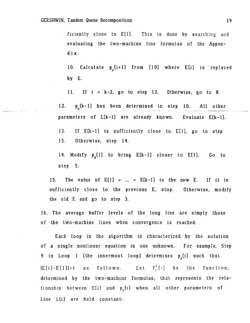
GERSHWIN, Tandem Queue Decomposition 19
ficiently close to E(l). This is done by searching and
evaluating the two-machine line formulas of the Appen-
dix.
10. Calculate pu(i+l) from [10) where E(i) is replaced
by E.
11. If i = k-2, go to step 12. Otherwise, go to 8.
12. pu[k-l) has been determined in step 10. All other
parameters of Lfk-l] are already known. Evaluate E(k-l].
13. If E(k-l]) is sufficiently close to E[1), go to step
15. Otherwise, step 14.
14. Modify pd(1] to bring E(k-l) closer to E(1). Go to
step 5.
15. The value of E[1] = ... = E[k-1) is the new E. If it is
sufficiently close to the previous E, stop. Otherwise, modify
the old E and go to step 3.
16. The average buffer levels of the long line are simply those
of the two-machine lines when convergence is reached.
Each loop in the algorithm is characterized by the solution
of a single nonlinear equation in one unknown. For example, Step
9 in Loop 1 (the innermost loop] determines pd(i] such that
IE (i)-E [ 1)[<c as follows. Let FI ( be the function,
determined by the two-machine formulas, that represents the rela-
tionship between E(i) and pdfi) when all other parameters of
Line L(i) are held constant:

GERSHWIN, Tandem Queue Decomposition 20
EMi) - F[lpdi)]) (29)
(The superscript 1 refers to Loop 1.) Let p(n-l(i)- and pn)([i) bed d
successive guesses of pd(i and let E(n-l ) and E(n) be the corres-
ponding values of E)i]. The Newton-Raphson method for choosing
the next guess pn+U(i) isd
_______ _ _-= - i)f pin)-E(i E) (30]Pd d dII dF(Pi )dF[pdM[i]
where the derivative is evaluated at n) Note that
E[1] is treated as a constant here. We approximate the deriva-
tive by the difference quotient
dFiPd([i)] E-n)(i) - En-i)31)-dp (i j(i) - pn_)(i)
and (30) becomes
pPn-+1)i)(E(n)(i) - E[l) - pcn)(i)(En-'')(i) - E1]))
d E(n)[i) - E(nl)(i)
Similarly, in Loop 2 we seek a value for pd (1) so that
IE(k-l)-E(l)c<E. In this loop, E(1) is a variable. Here we
apply Newton's method to the equation
E[k-1)-E[1) = F2(pd(1)) (33)
so that the iteration formula is

GERSHWIN, Tandem Queue Decomposition 21
PM[el)] p-[1(13n(E(m[(k-l] - E1]) - pm)[1)(E(m-l)hLk- - E(]))d ) Etn)(k-l) _ E(m)(1) - E(ml)(k-l) + E(m-l)1 ]
Finally, Loop 3 (the outermost loop) determines a value for
E that satisfies the Flow Rate-Idle Time and Resumption of Flow
equations as well as Conservation of Flow. Let e ( be the value
of E used in Step 3 (Resumption of Flow) and Step 6 [Flow Rate-
^(&Idle Time) in the tth iteration. Then let E be the value of
E(1) to which Loop 2 converges. We seek 6 such that
E = R. One possible iteration process is simply
?*~'I= E = F3[6C )] (35)
but again, the Newton-Raphson method appears to be more effi-
cient. The iteration formula is
,,( +_ -=(e-1F3(gf()) _ g(F3(g( -l) [36)
F3(g () - F3[gl )) 6
Note that in all three loops, two initial values are re-
quired. In all the examples in the following sections, E was
large in the initial iterations and was then reduced to 10- 8.
Analytical results on the iteration process are not avail-
able. Numerical experience suggests that when it converges, it
converges to a unique solution which agrees closely with simula-
tion and is independent of the initial guess. There have been
some cases in which the algorithm failed to converge. These were
lines in which a few machines had much larger values for r and p

GERSHWIN, Tandem Queue Decomposition 22
than the others, or where the lines were very long (more than 20
machines].
The speed of the algorithm is best measured by the number of
evaluations of a two-machine line. This is reported below for
many cases.

GERSHWIN, Tandem Queue Decomposition 23
3. NUMERICAL RESULTS--BEHAVIOR OF THE ALGORITHM
In this section, the behavior of the algorithm is described.
The issues investigated are those of accuracy and computational
effort. The behavior of transfer lines, as determined by this
method, is presented in Section 4.
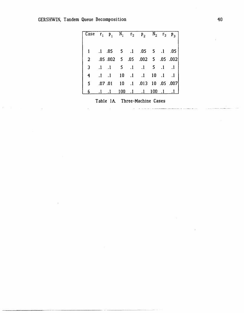
Three-Machine Cases
It is possible to compare the results of this algorithm with
exact results by using the method of Gershwin and Schick (1983).
Table 1A lists the parameters of a set of cases. These cases
represent a wide range of three-machine systems. Simulations
were also performed for comparison. Each simulation was run for
a total of 100,000 time units. The results are shown in Table
lB.
The approximate method produces results that are extremely
close to the exact values obtained by solving the Markov chain
exactly. The error is very small in the production rate E (less
than 0.02)} and only a little larger (less than 2.6Z) in the
average buffer levels. The approximate results are generally as
close or closer to exact as the simulation results.
The table also shows how efficient the method is. The eval-
uation of a two-machine transfer line is a very small computatio-
nal burden. Eighty-eight evaluations requires orders of magni-
tude less computer time than that required for the exact solution
or for the simulations. Note that Case 6 has buffers that are
too large for the exact method, but that the agreement with

GERSHWIN, Tandem Queue Decomposition 24
simulation is good.
Longer Lines
Exact methods are not available for systems of more than
three machines or for three-machine cases with very large buf-
fers. Consequently, other techniques are required to assess the
accuracy of the approximation. They include simulation and exact
qualitative results. The cases considered here represent a wide
. .---.------ range-of---.failure-probabilities,--repair--probabilities, and buffer
sizes. The results cover a wide range of production rates and
average buffer levels.
There is close agreement between the approximation and simu-
lation results. In most cases, production rates and buffer
levels agree to within a few percent. This remains true even for
large buffer capacities (over 100) and long lines [20 machines.)
There is no obvious trend indicating that the accuracy of the
approximation decreases as the line length increases.
Cases in which r = pi = .1
The number of evaluations of two-machine lines increases
with the length of the line. Figure 3 shows this for two sets of
cases in which repair and failure probabilities are all equal to
.1. Experience indicates that the number of evaluations ap-
pears to be O(k3 ), where k is the number of machines.
Most of the approximation and simulation results of this and
the next section were produced on the MIT Honeywell 68/DPS compu-
ter with the Multics operating system. All times indicated were
GERSHWIN, Tandem Queue Decomposition 25
for runs performed on this machine. Experience indicates that
the computer time for the analytic approximation method appears
to be much less than that of simulation.
Other runs -- both approximate and simulation -- were per-
formed on an IBM PC and a variety of compatible computers.
Table 2 shows the results of a set of cases with repair and
failure probabilities all equal to .1 and buffer sizes all equal
to 5. Production rates (E) are indicated for all cases; average
buffer levels and computer times are indicated for the 20-machine
line. Note the close agreement between approximate and simulated
production rates and average levels. Table 3 contains similar
results but with all buffer capacities equal to 10.
Reversibility and Symmetry.
Several authors have conjectured (Hillier and Boling, 1977)
or shown [Dattatreya, 1978; Muth, 1979; Ammar, 1980; Ammar and
Gershwin, 1981) that two tandem queueing systems which are the
reverse of one another have the same production rates. In addi-
tion (Ammar, 1980; Ammar and Gershwin, 1981), the average levels
of corresponding buffers are complementary.
Symmetric lines are their own reverses. The complementarity
property applies to symmetrically opposite buffers. That is, for
i = 1, ... , k-l,
ni + n ki = Ni = Nki. (37)
Furthermore, the average level in the middle buffer of a
GERSHWIN, Tandem Queue Decomposition 26
symmetric line with an odd number of buffers is equal to exactly
half the capacity of that buffer [Ammar, 1980). That is, if k is
even and i = k/2, [37) implies
k/2 = N/2 [38)
The results of the decomposition method agree with these
observations exactly. Simulation, however, produces only ap-
proximate agreement. These properties are exhibited in the last
case of the Table 2;, the first case of Table 3; Cases 1-4; 6; 14
and 15; 18 and 23; and 19 and 21.
Perturb'ed cases
Tables 4A and 4B contain a set of four-machine cases that
are close to three-machine cases already considered. It includes
machines that are nearly, but not quite, perfect. If those
machines were perfect, these cases would be the same as the
earlier cases. We expect the behavior of the perturbed cases to
be close to that of the others.
Case 7 was chosen to be close to Case 4. Case 7 is a four-
machine line whose second machine almost never fails. The first
two buffers of Case 7 have a total capacity which is equal to
that of B, of Case 4, and the other corresponding machines and
buffers are the same. The sum of the average levels of the first
two buffers of Case 7 is 5.977. This should be compared with the
average level of Bl of Case 4 which is 6.063. In addition,
5i, of Case 7 is not far from n2 of Case 4.

GERSHWIN, Tandem Queue Decomposition 27
Similarly, Case 8 was chosen to be close to Case 3. Here the
highly efficient machine is the last. The first three machines
and two buffers of Case 8 are identical to Case 3. The results
are also in close agreement. Furthermore, the level in the last
buffer can be explained.
Because the last machine nearly never fails, the last buffer
never has more than one piece in it. If it were initialized with
more than one piece, the number of pieces would diminish whenever
the third machine was down or the second buffer was empty. If
such a condition persisted, the third buffer would become empty.
Eventually, the third buffer would have exactly one piece if the
third machine were working and the second buffer were non-empty;
and it would be empty otherwise. That is, it would have one
piece whenever the three-machine subset was producing parts and
no pieces when it was not.
To calculate the expected level in the third buffer, we need
to know the fraction of time the subset is producing parts. We
do: it is the production rate of the three-machine subset. As a
consequence, the average number of parts in the last buffer [when
the last machine is almost perfectly reliable) is equal to the
production rate, in parts per time unit.
The simulation results also bear this out. Cases 4 and 9
are in the same relationship as Cases 3 and 8 and they demon-
strate this behavior.

GERSHWIN, Tandem Queue Decomposition 28
Comparison with Published Simulations
Cases 10-12 (Table SA] are a set of 5-machine lines from
example ([c of Ho, Eyler, and Chien (1979) and the simulation
results (production rates) of Table 5B are theirs (written in a
slightly different form). In each of these cases,
r,=.005, pi=.001, i=l, ..., 5
The approximate and simulation production rates are in good
agreement. Furthermore, both methods calculate production rates
for Case 12 which are greater than those for Case 11, which are
greater than those for Case 10.
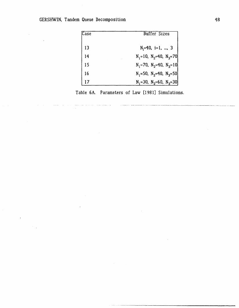
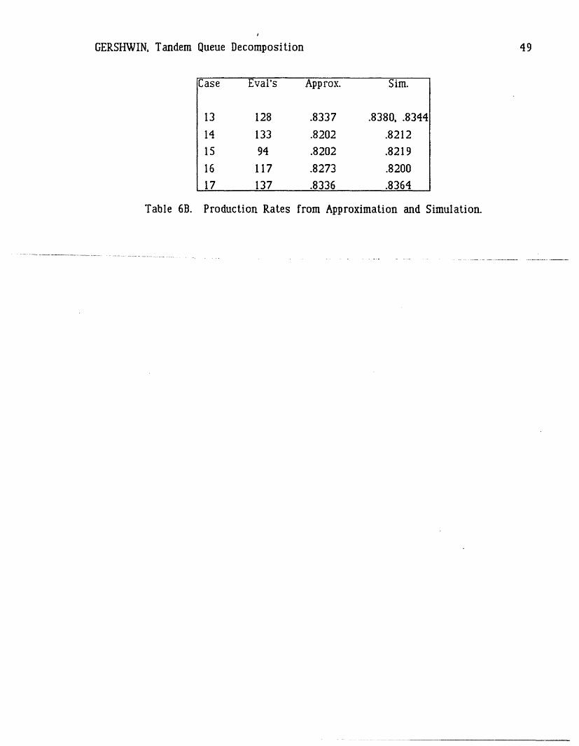
Cases 13-23 [Table 6A) are taken from Law (1981) and again
the simulation results (Table 6B) come from the cited paper.
These are all 4-machine lines in which
r,=.05, p,=.00S, i=l, ..., 4
The decomposition results are in close agreement with simu-
lated values. However, Law draws conclusions that are not sup-
ported by reversibility or decomposition results. Cases 13-17
are Buffer Allocations 1-5 of Table 4 of Law (1981). Law finds
Allocations I and 5 to be statistically indistinguishable and to
have a greater production rate than Allocations 2, 3, and 4,
which are also indistinguishable. However, we find that Alloca-
tions 2 and 3 (i.e., Cases 14 and 15) are the same (due to rever-
sibility). Their production rate is less than that of Allocation
4 (Case 16) which is less than that of Allocation 5 (Case 17)
which is less than that of Allocation I (Case 13).

GERSHWIN, Tandem Queue Decomposition 29
Cases 18-23 (Table 7) are Patterns 1-6 of Table 2 of Law
(1981). Law is seeking to find the best sequence of four ma-
chines of which two have high efficiency (H) and two have low
efficiency (L). The parameters of the H machines are p=.0025 and
r=.05. The L machines have p=.02 and r=.05. The three buffers
each have capacity 19 in all cases. Law finds that the patterns,
in order of production rate, are
(23,22), 21, 18, 19, 20.
using the case numbers of this paper. That is, Cases 23 and 22
cannot be distinguished, but their production rate is less than
that of Case 21, and so forth.
We find instead the following order:
22, (18,23), ( 19,21]), 20.
The cases that we find indistinguishable are the reverses of one
another.
Cases with Different Machines
Many of the lines treated here have had identical machines.
Table 8B shows the results of two cases with different machines,
whose parameters are listed in Table 8A. These are six- and
twelve-machine cases that consist of the three machines of Case
5, doubled and quadrupled. The buffers are all of capacity 10.
The simulation and approximation results are in close agreement.

GERSHWIN, Tandem Queue Decomposition 30
4. NUMERICAL RESULTS--BEHAVIOR OF TRANSFER LINES
Figure 4 demonstrates how the production rate varies with
the length of the line for two sets of cases. It is not surpri-
sing that production rates decrease as lines grow. This graph
does not, however, settle the question of whether the production
rate approaches zero as the length goes to infinity.
Figure 5 shows how material is distributed in the buffers
for two twenty-machine cases. Note how the average buffer level
in the tenth buffer is equal to half the buffer's capacity. This
is due to the symmetry of both cases, as discussed above. All
the other buffers exhibit complementarity. For example, in the
case where Ni=10 for all i, fi3 +fi17=10.
Cases 3, 4, and 6 of Section 3 show that as the buffer sizes
increase, the production rate increases. In addition, the ave-
rage buffer levels, as a fraction of capacities, approach .5. In
general, production rate increases with buffer capacity, but
buffer levels do not always approach half of buffer capacity as
capacity increases.
Figure 6 shows the effect of increasing total buffer space
and the effect of varying the distribution of buffer space. A
system of nine identical machines with parameters r=.019 and
p=.001 is considered. In one set of cases, there are eight
buffers with equal capacities. In the other, there are two
buffers with equal capacities, located between the third and
fourth machines and between the sixth and seventh machines.

GERSHWIN, Tandem Queue Decomposition 31
(Each set of three machines is equivalent to one machine with
parameters r=.01898 and p=.002997.)
The reason the 8-buffer lines are better than the 2-buffer
lines when the space is large is that the production rate is
limited by the least productive machine. In the former case, the
limiting efficiency is .95; in the latter it is .8636 since each
set of three machines acts like a single machine. The behavior
when the buffer space is small may be due to the model of block-
ing and starvation used here; with other models, the 8-buffer
distribution may always be better than the 2-buffer distribution.
Note that the total average buffer levels are the same in the two
sets of cases: half the total capacity (due to symmetry).
The facts that Case 20 is the best of Cases 18-23, that 13
and 17 are the best of 13-17, and that 33 is the best of 31-33
may be instances of the "bowl phenomenon" (Hillier and Boling,
1966), which is that, for maximal production rate, more buffer
space should be allocated to the middle of a line.

GERSHWIN, Tandem Queue Decomposition 32
5. CONCLUSIONS AND FURTHER RESEARCHA new method has been found for the analysis of tandem
queuing systems with finite buffers in which blocking is impor-
tant. Exact and simulation results indicate that the method,
while approximate, is quite accurate. Current research is aimed
at extending this work in two directions: other service process
behavior, such as reliable and unreliable machines with exponen-
tial and other processing time distributions (Choong and Ger-
shwin, 1985; Gershwin, 1985); and assembly/disassembly networks
[Gershwin, 1986). Future efforts will be devoted to systems such
as Jackson-like networks with blocking.
Research is needed to determine precisely the performance of
this method. That is, analytic techniques rather than only
numerical experiments should be used to develop bounds on the ac-
curacy of the method and to determine convergence properties of
the algorithm.
GERSHWIN, Tandem Queue Decomposition 33
REFERENCEST. Altiok (1982), "Approximate Analysis of Exponential Tandem
Queues with Blocking," European Journal of Operations Re-
search, Vol. 11, 1982.
M. H. Ammar (1980], "Modelling and Analysis of Unreliable Manu-
facturing Assembly Networks with Finite Storages," MIT Laboratory
for Information and Decision Systems Report LIDS-TH-1004.
M. H. Ammar and S. B. Gershwin (1981), "Equivalence Relations in
Queuing Models of Manufacturing," Proceedings of the Nineteenth
IEEE Conference on Decision and Control.
J. A. Buzacott (1967), "Markov Chain Analysis of Automatic Trans-
fer Lines with Buffer Stock," Ph.D. Thesis, Department of Engi-
neering Production, University of Birmingham.
J. A. Buzacott (1967), "Automatic Transfer Lines with Buffer
Stocks," International Journal of Production Research, Vol.
6.
Y. F. Choong and S. B. Gershwin [1985), "A Decomposition Method
for the Approximate Evaluation of Capacitated Transfer Lines with
Unreliable Machines and Random Processing Times," MIT Laboratory
for Information and Decision Systems Report LIDS-P-1476; to
appear in IIE Transactions.
P. Coillard and J.-M. Proth (1983), "Sur L'Effet des Stocks
Tampons Dans Une Fabrication en Ligne," INRIA Rapports de Re-
cherche, Institut National de Recherche en Informatique et en
GERSHWIN, Tandem Queue Decomposition 34
Automatique, Domaine de Voluceau, Roquencourt, Le Chesnay,
France.
E. S. Dattatreya (1978), "Tandem Queueing Systems with Blocking,"
Ph. D. thesis, Department of Industrial Engineering and Opera-
tions Research, University of California, Berkeley.
S. B. Gershwin (1984), "An Efficient Decomposition Method for the
Approximate Evaluation of Production Lines with Finite Storage
------- Space-,"-- in--- Analysis--and--Optimization--of-- Systems, Proceedings
of the Sixth International Conference on Analysis and Optimi-
zation of Systems, Part 2, Volume 63 of Lecture Notes in
Control and Information Sciences, Springer-Verlag, 1984.
S. B. Gershwin (1985), "Representation and Analysis of Transfer
Lines with Machines that have Different Processing Rates," MIT
Laboratory for Information and Decision Systems Report LIDS-P-
1446; to appear in Annals of Operations Research.
S. B. Gershwin (1986), "Assembly/Disassembly Systems: An Effi-
cient Decomposition Algorithm for Tree-Structured Networks," MIT
Laboratory for Information and Decision Systems Report LIDS-P-
1579, July, 1986.
S. B. Gershwin and 0. Berman (1981), "Analysis of Transfer Lines
Consisting of Two Unreliable Machines with Random Processing
Times and Finite Storage Buffers," AIIE Transactions Vol.
13, No. 1, March 1981.
S. B. Gershwin and I. C. Schick (1983), "Modeling and Analysis of
Three-Stage Transfer Lines with Unreliable Machines and Finite
GERSHWIN, Tandem Queue Decomposition 35
Buffers," Operations Research, Vol. 31, No.2, pp 354-380,
March-April 1983.
L. E. Hanifin, J. A. Buzacott, and K. S. Taraman (1975], "A
Comparison of Analytical and Simulation Models of Transfer
Lines," SME Technical Paper EM75-374, Society of Manufacturing
Engineers, 20501 Ford Road, Dearborn, Michigan 48128.
F. S. Hillier and R. W. Boling (1966), "The _Effect of _ Some Design
Factors on the Efficiency of Production Lines with Variable
Operation Times," Journal of Industrial Engineering, Vol.
17, No. 12, December, 1966.
F. S. Hillier and R. Boling (1977), "Toward Characterizing the
Optimal Allocation of Work in Production Lines with Variable
Operation Times," in Advances in Operations Research, Proceedings
of EURO II, Marc Reubens, Editor; North-Holland, Amsterdam.
Y. C. Ho, M. A. Eyler, and T. T. Chien (1979), "A Gradient
Technique for General Buffer Storage Design in a Production
Line," International Journal of Production Research, Vol.
17, No. 6, pp 557-580, 1979.
G. C. Hunt [1956)], "Sequential Arrays of Waiting Lines," Ope-
rations Research, Volume 4, 1956.
M. A. Jafari (1982), Ph. D. Thesis proposal, Syracuse University.
S. S. Law (1981), "A Statistical Analysis of System Parameters in
Automatic Transfer Lines," International Journal of Production
Research, Vol. 19, No. 6, pp 709-724, 1981.

GERSHWIN, Tandem Queue Decomposition 36
E. J. Muth (1979), "The Reversibility Property of Production
Lines," Management Science, Vol.25, No. 2.
T. Ohmi (1981) "An Approximation for the Production Efficiency of
Automatic Transfer Lines with In-Process Storages," AIIE
Transactions, Volume 13, No. 1, March 1981.
I. C. Schick and S. B. Gershwin (1978), "Modelling and Analysis
of Unhreliable--Transfer-Lin-es-- -with--Finite Interstage Buffers,"
Massachusetts Institute of Technology Electronic Systems Labora-
tory Report ESL-FR-834-6, September, 1978.
R. Suri and G. Diehl (1983], "A Variable Buffer-Size Model and
its Use in Analyzing Closed Queuing Networks with Blocking,"
Harvard University, Division of Applied Sciences, September,
1983.
Y. Takahashi, H. Miyahara, and T. Hasegawa (1980), "An Approxima-
tion Method for Open Restricted Queuing Networks," Operations
Research, Vol. 28, No.3, Part I, May-June 1980.
P. Vanderhenst, F. V. Van Steelandt, and L. F. Gelders (1981),
"Efficiency Improvement of a Transfer Line Via Simulation," Ka-
tholieke Universiteit Leuven, Faculteit Toegepaste Wetenschappen
Afdeling Industrieel Beleid, Belgium; Report 81-04, January 1981.

GERSHWIN, Tandem Queue Decomposition 37
APPENDIXSteady-State Probabilities and Performance Measures for Two-
Machine Lines
In the following, p(n, a l , 0 2) is the probability that
there are n parts in the buffer and that Mi is in state a i.
These probabilities are taken from Gershwin and Schick (1983).
p[O,O,O) = O
p(oo,l) = C X r I + r2 - r 1r 2 - rip2
p(0{l,0) : 0 rIP2
p(O,l,l] =0
p[(l,OO) = C X
p(1,0,1) = C X Y2
p(1,1,O) =
p1,,l1] =C X rl + r2 - rlr2 - rlp2
P2 p1 + p2 - P IP 2 - rip2
p(N-l,O,0] = C X-'
p(N-l,O,l) = 0
p(N-l,l,O) = C XN-' Y 1
pC-,,l _- C X N- rl + - rr 2 -rr2 r2P1 pi + P 2 - PIP 2 - P"r2
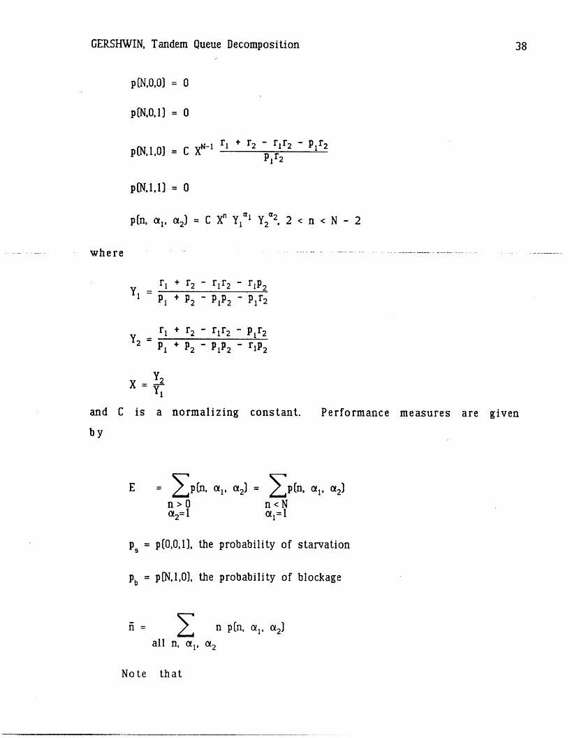
GERSHWIN, Tandem Queue Decomposition 38
p([N,O,O] = 0
p(N,O,l) = 0
p(N,l,0) = C XN -I rl + r 2 - rf r2 - plr 2
p(N,l,1] = 0
p(n, al, c2 ) = C Xn y al Y2 2, 2 < n < N - 2
where
r1 + - rFr 2 - rlP 2
P1 + P2 - PP 2 - Plr 2
rl + r2 - rlr2 - Plr 2
2 P + P2 - PP2 - rip2
X Y2
yi
and C is a normalizing constant. Performance measures are given
by
E = p[n, a, a 2 ) = Sp(n, a 1, a 2 )
n>O n<No2 =l al=l
PS = p(O,O,1), the probability of starvation
Pb = p(N,l,0), the probability of blockage
ni= _ n p(n,. o1, a 2)
all n, at, a 2
Note that

GERSHWIN, Tandem Queue Decomposition 39
E = e (1 - pb]
= e2 (1 -PS).
GERSHWIN, Tandem Queue Decomposition 40
Case rI pi Nl r 2 P2 N2 r3 p3
1 .1 .05 5 .1 .05 5 .1 .05
2 .05 .002 5 .05 .002 5 .05 .002
3 .1 .1 5 .1 .1 5 .1 .1
4 .1 .1 10 .1 .1 10 .1 .1
5 .07 .01 10 .1 .013 10 .05 .007
6 .1 .1 100 .1 .1 100 .1 .1
Table 1A. Three-Machine Cases

GERSHWIN, Tandem Queue Decomposition 41
E 2l Evaluations
Case 1
Approximate Results .4542 3.088 1.912 70Exact Results .4545 3.063 1.937Simulation 1 .4567 3.030 1.953Simulation 2 .4554 3.034 1.877Simulation 3 .4514 3.072 1.969
Case 2
Approximate Results .8993 3.001 1.999 32Exact Results .8992 2.987 2.013Simulation 1 .9031 3.087 2.024Simulation 2 .9030 3.135 2.056Simulation 3 .8883 2.998 1.982
Case 3
Approximate Results .3105 3.101 1.899 68Exact Results .3109 3.075 1.925Simulation 1 .3075 3.060 1.918Simulation 2 .3126 3.096 1.912Simulation 3 .3109 3.086 1.926
Case 4
Approximate Results .3563 6.063 3.937 64Exact Results .3556 6.035 3.965Simulation 1 .3544 6.089 3.908Simulation 2 .3572 6.109 4.024Simulation 3 .3552 6.011 3.903
Case 5
Approximate Results .7546 6.182 3.349 86Exact Results .7539 6.120 3.437Simulation 1 .7548 6.107 3.443Simulation 2 .7478 6.412 3.523Simulation 3 .7558 6.074 3.310
Case 6
Approximate Results .4722 56.60 43.40 88Simulation .4676 58.59 45.71
Table lB. Results of Three-Machine Cases

GERSHWIN, Tandem Queue Decomposition 42
Line length, k Quantity Eval's Approx. Sim. 1 Sim. 2
4 E 116 .2806 .2830 .28095 238 .2630 .2632 .26476 399 .2516 .2514 .25197 583 .2438 .2418 .24588 996 .2382 .2365 .233210 2030 .2309 .2306 .225113 4110 .2248 .2212 .219317 7705 .2206 .2119 .2132
20 E 9467 .2188 .2107 .2117i1 3.902 3.850 3.909
i5 2.935 3.106 2.856
ilo 2.500 2.684 2.543nl9 1.098 1.086 1.119
time 6.897 248.169 247.685
Table 2. Performance of Systems with N=5.

GERSHWIN, Tandem Queue Decomposition 43
Line length, k Quantity Eval's Approx. Sim. 1 Sim. 2
4 E 131 .3352 .3341 .3390fil 6.535 6.604 6.556
ni2 5.000 5.133 4.992
113 3.465 3.637 3.564
5 E 234 .3228 .3232 .31756 386 .3149 .3075 .31277 614 .3095 .3033 .30578 1387 .3056 .2970 .295710 1899 .3006 .2934 .2910.... 13 3521 .2964 .2830 .286117 10389 .2936 .2768 .2813
20 E 17185 .2924 .2774 .2759time 12.155 262.188 261.079
Table 3. Performance of Systems with N=10.

GERSHWIN, Tandem Queue Decomposition 44
Case Parameters
7 ri=.l i=1, ., 4
pl=p3=p4=.1, p2=.000001N1=N2=5, N3=10
8 ri=.l, i=l, ..., 4
pl=p2=p3=.1, p4=.000001Ni=N2=N3=5
9 ri=. 1, i= 1, .... 4pl=P2=P3=. , p 4=.000001
Nl=N2=N3=10
-- Table-4A.-Parameters of Perturbed Cases.
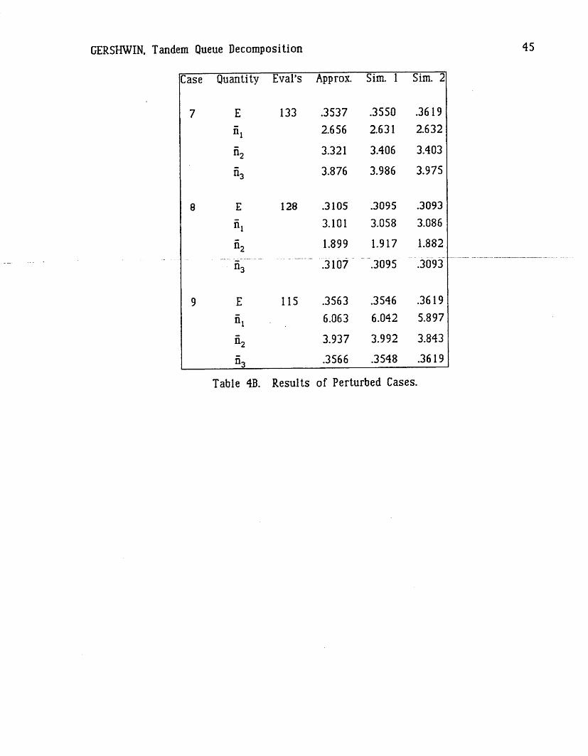
GERSHWIN, Tandem Queue Decomposition 45
Case Quantity Eval's Approx. Sint 1 Sim. 2
7 E 133 .3537 .3550 .3619
ii1 2.656 2.631 2.632
n2 3.321 3.406 3.403
53 3.876 3.986 3.975
8 E 128 .3105 .3095 .3093
iil 3.101 3.058 3.086
112 1.899 1.917 1.882
-n3 .3107 .3095 .3093
9 E 115 .3563 .3546 .3619
fll 6.063 6.042 5.897
fi2 3.937 3.992 3.843
fl3 .3566 .3548 .3619
Table 4B. Results of Perturbed Cases.

GERSHWIN, Tandem Queue Decomposition 46
Case Buffer Sizes
10 Ni=100, i=l, ..., 4
11 N 1=80, N2=122, N3=126, N4=72
12 N1=60, N2=146, N3=142, N4=52
Table SA. Parameters of Ho, Eyler, Chien (1979) Simulations.

GERSHWIN, Tandem Queue Decomposition 47
Case Eval's Approx. Sim
10 293 .6007 .5927
11 289 .6034 .5948
12 295 .6045 .5958
Table SB. Production Rates from Approximation and Simulation.
GERSHWIN, Tandem Queue Decomposition 48
Case Buffer Sizes
13 Ni=40, i=l, ..., 3
14 Nl=10, N2=40, N3=70
15 N1=70, N2=40, N3=10
16 N1=50, N2=40, N3=50
17 N1=30, N2=60, N3=30
Table 6A. Parameters of Law (1981) Simulations.
GERSHWIN, Tandem Queue Decomposition 49
Case Eval's Approx. Sim.
13 128 .8337 .8380, .8344
14 133 .8202 .821215 94 .8202 .8219
16 117 .8273 .820017 137 .8336 .8364
Table 6B. Production Rates from Approximation and Simulation.

GERSHWIN, Tandem Queue Decomposition 50
Case SequenceCase SMachince Eval~s Approx. Simr
18 LLHH 898 .6363 .6534
19 LHLH 111 .6707 .6651
20 LHHL 122 .6906 .6767
21 HLHL 148 .6707 .6442
22 HLLH 137 .6351 .6192
-__23 . ---- HHLL-' 146 .6363 .6173
Table 7. Sequences from Law (1981) and Results.

GERSHWIN, Tandem Queue Decomposition 51
Case Line Length, k Parameters
24 6 r1=r4=.07, r 2=r5=.l, r 3=r6=.05pl=p4=.01, P2=p5=.013, p 3=p6=.007
Ni=10, i=l, ..., 5
25 12 rx=r4=r7=rjo=.07r 2=r 5=r8=rl=. 1,r 3=r 6=r 9=rl2=.05,
P =p4 =p7=p O=' 0 1,P2=P5=P8=P= l=.013,P3=P 6=Pg=PI2= 007,N=Table A Parameters of, i=nes with Differen...t Machines.11
Table 8A. Parameters of Lines with Different Machines.

GERSHWIN, Tandem Queue Decomposition 52
Case Eval's Approx Sim
24 1582 .6692 .6684
25 4455 .6098 .5916
Table 8B. Results from Lines with Different Machines.
Page 53
Line L
MI 8 M2 82 M3 83 M4 84 M 5 85 M6 86 M7
r,, P N1 r2,p rP N2 r, N 4 N4 rS,ps N5 r6,p6 N6 r7,P7
Figure 1
lI1-CG-m Line L(C)
r(:l),psl) N1 rd(1),pd(1)
M,(2) 22 M (2)
Line L(2)O :
ru(2),pu(2) N2 rd(2!,Pd- 2 )
MU3) 83 M.(3)Line L(3) 1-0 -
ru(3),Pu(3) N3 r~( 3 ),pd(3 )
M,(4) E4 Mj(4)
Line L(4) "--r _
ru(4),pu(4) N4 rd(4 ),pd(4 )
M(5) C. MC5)
Line L(5) "r ', ]
ru(),pu,) N r),p( 5 )
Mu,() sE Md( 6 )Line L()
ru(6),p,(6) N rd(6),pd(6)
Figur- '2

Page 54
100,000
en 0C 10,000 0 -
V-c-~~~~~ki_ 4
!
CaC
1000
- -- ,p--- i- 1i, , , 1
. _ _N i-' '2 M ' 2-t
ixiu~~-r of Me cchins k
Figure 3

Page 55
Production Rate E, Parts/Cycleo) i Fo Fo ro Fo Fo o ~ a b L
-- U O c (D -- CO ;: 0 0 a .
. i I i i I I I I i
U-IC)
.- /-a-
?L | _ ~, . /.4I ,--
r~ X O - -a
UII
0, - CO~~~r~~~~~~~~~~~~~~~~~~~~~~~~~~~~~~~~~i~~~~~~~~~~~~~~~~
C)~~~~~~~~~~~~~~~~~~~~~~~~~~~~~~~~~~~~~~~~~~~~~·m.

Page 56
Average Buffer Level, N i =5
Co o
0 o'10 I0oC _
0 . rI cI II II--. , I......._ I
I-
6 o 0_0 0 0 0

Page 57
Efficiency0 0 o 0 0 0CI 0
i I I
i
-,4
OC
0f X
0
0 ' \\, a"
o- ° C/ /0~~~~~~~~13)~~~~~~~~~~~~~~~~~l XO·3 '~ .. ~ ... ,,~~~~~~~~~~~~~~~~ro.. \ 1
0 -"""~~~0lc/
O~~~~~~~~o