Dirty Paper Coding - Electrical and Computer Engineering · Dirty Paper Coding Gwanmo Ku Adaptive...
33
Dirty Paper Coding Gwanmo Ku Adaptive Signal Processing and Information Theory Research Group Nov. 7, 2012
Transcript of Dirty Paper Coding - Electrical and Computer Engineering · Dirty Paper Coding Gwanmo Ku Adaptive...

Dirty Paper Coding
Gwanmo Ku
Adaptive Signal Processing and Information Theory Research Group
Nov. 7, 2012

Outline
Introduction
Writing on Dirty Paper
System Model & Channel Capacity
Achievable Rate Region
Encoding & Decoding
Achievability Proof
Example of Dirty Paper Coding
2/22

Outline
Introduction
Writing on Dirty Paper
System Model & Channel Capacity
Achievable Rate Region
Encoding & Decoding
Achievability Proof
Example of Dirty Paper Coding

Writing on Dirty Paper (Costa, 83)
4/22
Costa’s Idea
⊕ ⊕ Encoder Decoder
𝐒 ∼ 𝓝(𝟎,𝑸) 𝒁 ∼ 𝓝(𝟎,𝑵)
𝑊 𝒀 𝑊
𝒀 = 𝑿 + 𝑺 + 𝒁
State noise source (AWGN)
Known at Encoder Channel noise channel (AWGN)
𝑿
𝟏
𝟐 𝐥𝐧 (𝟏 +
𝑷
𝑵)
𝟏
𝟐 𝐥𝐧 (𝟏 +
𝑷
𝑵 + 𝑸)
State 𝑆 does not effect the capacity
Average power constraint
𝑷
Capacity
Writing on Dirty Paper (Costa, 83)
5/22
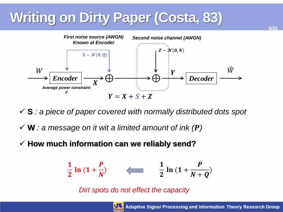
S : a piece of paper covered with normally distributed dots spot
W : a message on it wit a limited amount of ink (𝑷)
How much information can we reliably send?
𝟏
𝟐 𝐥𝐧 (𝟏 +
𝑷
𝑵)
𝟏
𝟐 𝐥𝐧 (𝟏 +
𝑷
𝑵 + 𝑸)
Dirt spots do not effect the capacity
⊕ ⊕ Encoder Decoder
𝐒 ∼ 𝓝(𝟎,𝑸) 𝒁 ∼ 𝓝(𝟎,𝑵)
𝑊 𝒀 𝑊
𝒀 = 𝑿 + 𝑺 + 𝒁
First noise source (AWGN)
Known at Encoder Second noise channel (AWGN)
𝑿 Average power constraint
𝑷

Writing on Dirty Paper (Costa, 83)
6/22
Practical Importance
Diversity without capacity loss
Layering by dirt spots (Watermarking)
Extension to MIMO case for Diversity
Centered at on 𝐒𝟏 Centered at on 𝐒𝟐

Outline
Introduction
Writing on Dirty Paper
System Model & Channel Capacity
Achievable Rate Region
Encoding & Decoding
Achievability Proof
Example of Dirty Paper Coding

Writing on Dirty Paper
8/22
System Model
Capacity
𝟏
𝟐 𝐥𝐧 (𝟏 +
𝑷
𝑵)
𝟏
𝟐 𝐥𝐧 (𝟏 +
𝑷
𝑵 + 𝑸)
State 𝑆 does not effect the capacity
⊕ ⊕ Encoder Decoder
𝐒 𝐙
𝑊
𝑆𝑛
𝑿𝒏 𝒀𝒏 𝑊
𝒀 = 𝑿 + 𝑺 + 𝒁
State
S ∼ 𝒩(0, 𝑄)
Channel
Z ∼ 𝒩(0, 𝑁)
1
𝑛 𝑋𝑖
2 ≤ 𝑃
𝑛
𝑖=1
𝑊 ∈ {1,… , 𝑒𝑛𝑅}
Independent
Known at
Encoder
Capacity Region
9/22
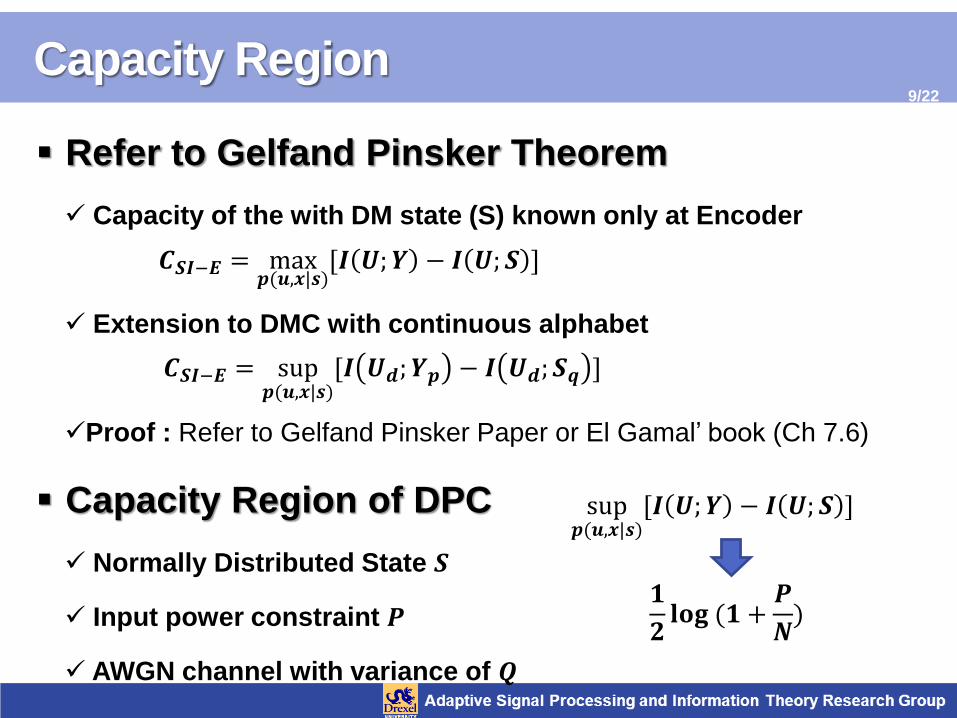
Refer to Gelfand Pinsker Theorem
Capacity of the with DM state (S) known only at Encoder
Extension to DMC with continuous alphabet
Proof : Refer to Gelfand Pinsker Paper or El Gamal’ book (Ch 7.6)
Capacity Region of DPC
Normally Distributed State 𝑺
Input power constraint 𝑷
AWGN channel with variance of 𝑸
𝑪𝑺𝑰−𝑬 = max𝒑(𝒖,𝒙|𝒔)
[𝑰 𝑼; 𝒀 − 𝑰 𝑼; 𝑺 ]
sup𝒑(𝒖,𝒙|𝒔)
[𝑰 𝑼; 𝒀 − 𝑰 𝑼; 𝑺 ]
𝟏
𝟐𝐥𝐨𝐠 (𝟏 +
𝑷
𝑵)
𝑪𝑺𝑰−𝑬 = sup𝒑(𝒖,𝒙|𝒔)
[𝑰 𝑼𝒅; 𝒀𝒑 − 𝑰 𝑼𝒅; 𝑺𝒒 ]
Encoding
10/22
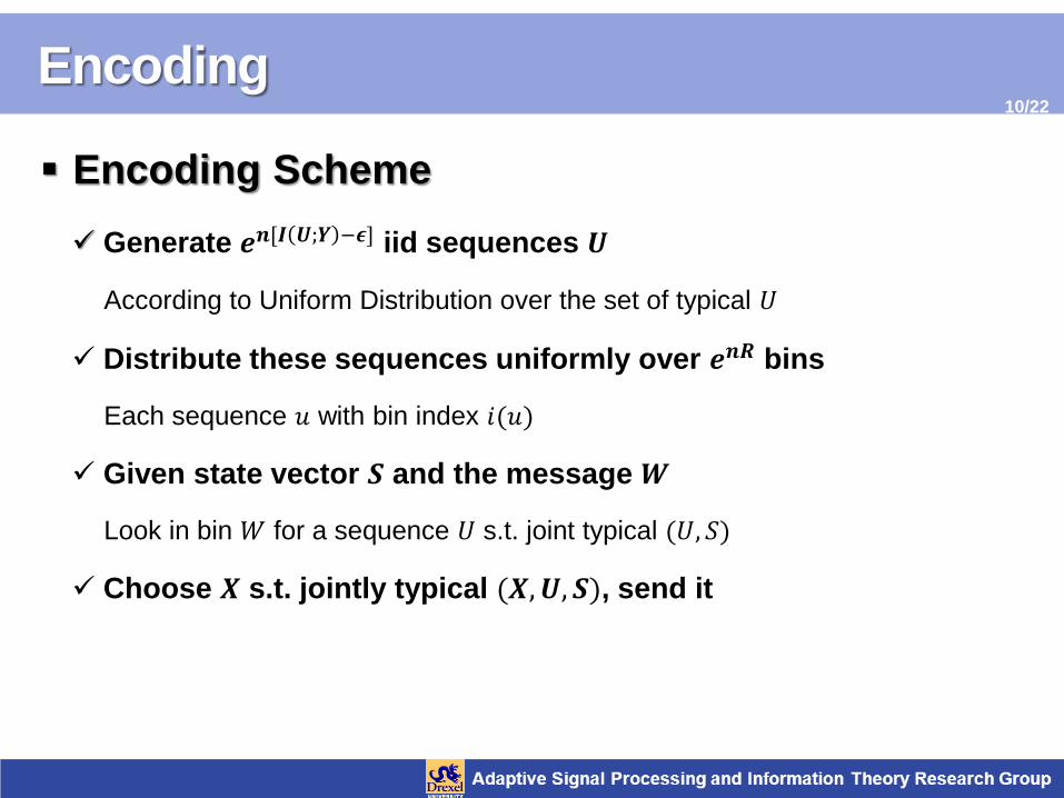
Encoding Scheme
Generate 𝒆𝒏[𝑰 𝑼;𝒀 −𝝐] iid sequences 𝑼
According to Uniform Distribution over the set of typical 𝑈
Distribute these sequences uniformly over 𝒆𝒏𝑹 bins
Each sequence 𝑢 with bin index 𝑖(𝑢)
Given state vector 𝑺 and the message 𝑾
Look in bin 𝑊 for a sequence 𝑈 s.t. joint typical (𝑈, 𝑆)
Choose 𝑿 s.t. jointly typical (𝑿,𝑼, 𝑺), send it

Decoding
11/22
Decoding Scheme
Look for unique sequence 𝑼 s.t. jointly typical (𝑼, 𝒀)
Declare Error
More than one or no such sequence exist
Set the estimate 𝑾
Equal to the index of bin containing the obtained sequence 𝑈
If 𝑹 < 𝑰 𝑼; 𝒀 − 𝑰 𝑼; 𝑺 − 𝝐 − 𝜹
The probability of error averaged over all codes
decrease exponentially to zero as 𝑛 → ∞
Achievability Proof
12/22
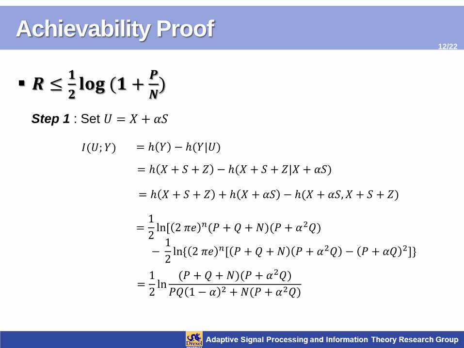
𝑹 ≤𝟏
𝟐𝐥𝐨𝐠 (𝟏 +
𝑷
𝑵)
Step 1 : Set 𝑈 = 𝑋 + 𝛼𝑆
𝐼(𝑈; 𝑌) = ℎ 𝑌 − ℎ(𝑌|𝑈)
= ℎ 𝑋 + 𝑆 + 𝑍 − ℎ(𝑋 + 𝑆 + 𝑍|𝑋 + 𝛼𝑆)
= ℎ 𝑋 + 𝑆 + 𝑍 + ℎ 𝑋 + 𝛼𝑆 − ℎ(𝑋 + 𝛼𝑆, 𝑋 + 𝑆 + 𝑍)
=1
2ln[ 2 𝜋𝑒 𝑛(𝑃 + 𝑄 + 𝑁)(𝑃 + 𝛼2𝑄)
− 1
2ln{ 2 𝜋𝑒 𝑛[ 𝑃 + 𝑄 + 𝑁 𝑃 + 𝛼2𝑄 − 𝑃 + 𝛼𝑄 2]}
=1
2ln(𝑃 + 𝑄 + 𝑁)(𝑃 + 𝛼2𝑄)
𝑃𝑄 1 − 𝛼 2 + 𝑁(𝑃 + 𝛼2𝑄)

Achievability Proof
13/22
𝐼(𝑈; 𝑆) = ℎ 𝑈 − ℎ(𝑈|𝑆)
= ℎ 𝑋 + 𝛼𝑆 − ℎ(𝑋 + 𝛼𝑆|𝑆)
= ℎ 𝑋 + 𝛼𝑆 + ℎ 𝑋
=1
2ln[ 2 𝜋𝑒 𝑛(𝑃 + 𝛼2𝑄)] −
1
2ln[ 2 𝜋𝑒 𝑛𝑃]
=1
2ln(𝑃 + 𝛼2𝑄)
𝑃
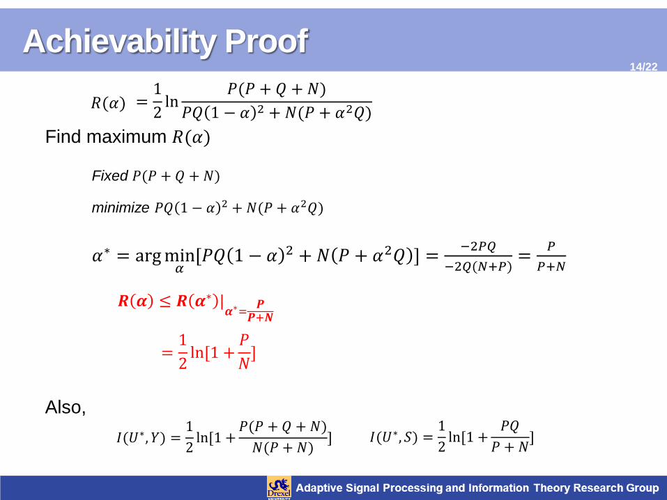
Let 𝑅 𝛼 = 𝐼 𝑈; 𝑌 − 𝐼(𝑈; 𝑆),
𝑅(𝛼) =1
2ln
𝑃(𝑃 + 𝑄 + 𝑁)
𝑃𝑄 1 − 𝛼 2 + 𝑁(𝑃 + 𝛼2𝑄)
𝐼(𝑈∗, 𝑆) =1
2ln[1 +
𝑃𝑄
𝑃 + 𝑁]
Achievability Proof
14/22
Find maximum 𝑅(𝛼)
Fixed 𝑃(𝑃 + 𝑄 + 𝑁)
minimize 𝑃𝑄 1 − 𝛼 2 + 𝑁(𝑃 + 𝛼2𝑄)
𝛼∗ = argmin𝛼[𝑃𝑄 1 − 𝛼 2 + 𝑁 𝑃 + 𝛼2𝑄 ] =
−2𝑃𝑄
−2𝑄(𝑁+𝑃)=
𝑃
𝑃+𝑁
Also,
𝑅(𝛼) =1
2ln
𝑃(𝑃 + 𝑄 + 𝑁)
𝑃𝑄 1 − 𝛼 2 + 𝑁(𝑃 + 𝛼2𝑄)
𝑹 𝜶 ≤ 𝑹 𝜶∗ |𝜶∗=
𝑷𝑷+𝑵
𝐼(𝑈∗, 𝑌) =1
2ln[1 +
𝑃(𝑃 + 𝑄 + 𝑁)
𝑁(𝑃 + 𝑁)] 𝐼(𝑈∗, 𝑆) =
1
2ln[1 +
𝑃𝑄
𝑃 + 𝑁]
=1
2ln[1 +
𝑃
𝑁]

Achievability Proof
15/22
Rate Regions and Capacity
𝑹(𝜶∗)
Encoding & Decoding with 𝜶∗
16/22
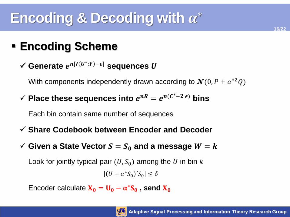
Encoding Scheme
Generate 𝒆𝒏[𝑰 𝑼∗;𝒀 −𝝐] sequences 𝑼
With components independently drawn according to 𝓝(0, 𝑃 + 𝛼∗2𝑄)
Place these sequences into 𝒆𝒏𝑹 = 𝒆𝒏(𝑪∗−𝟐 𝝐) bins
Each bin contain same number of sequences
Share Codebook between Encoder and Decoder
Given a State Vector 𝑺 = 𝑺𝟎 and a message 𝑾 = 𝒌
Look for jointly typical pair (𝑈, 𝑆0) among the 𝑈 in bin 𝑘
𝑈 − 𝛼∗𝑆0 𝑆′0 ≤ 𝛿
Encoder calculate 𝐗𝟎 = 𝐔𝟎 − 𝛂∗𝐒𝟎 , send 𝐗𝟎

Encoding & Decoding
17/22
Decoding Scheme
Receive 𝒀 = 𝒀𝟎
Look for a sequence 𝑈 s.t jointly typical (𝑈, 𝑌0)
Declare Error
More than one or no such sequence
Find 𝑈0
Set the estimate 𝑾
Equal to the index of bin containing this sequence
The probability of error averaged over random choice of code
decrease exponentially to zero as 𝑛 → ∞
Conclusion of DPC
18/22
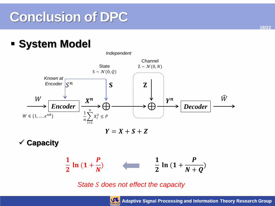
System Model
Capacity
𝟏
𝟐 𝐥𝐧 (𝟏 +
𝑷
𝑵)
𝟏
𝟐 𝐥𝐧 (𝟏 +
𝑷
𝑵 + 𝑸)
State 𝑆 does not effect the capacity
⊕ ⊕ Encoder Decoder
𝐒 𝐙
𝑊
𝑆𝑛
𝑿𝒏 𝒀𝒏 𝑊
𝒀 = 𝑿 + 𝑺 + 𝒁
State
S ∼ 𝒩(0, 𝑄)
Channel
Z ∼ 𝒩(0, 𝑁)
1
𝑛 𝑋𝑖
2 ≤ 𝑃
𝑛
𝑖=1
𝑊 ∈ {1,… , 𝑒𝑛𝑅}
Independent
Known at
Encoder

Outline
Introduction
Writing on Dirty Paper
System Model & Channel Capacity
Achievable Rate Region
Encoding & Decoding
Achievability Proof
Example of Dirty Paper Coding

Example of DPC
20/22
DPC for Gaussian BC
Assumptions
𝒀𝟏 = 𝑿 + 𝑺𝟏 + 𝒁𝟏
𝒀𝟐 = 𝑿 + 𝑺𝟐 + 𝒁𝟐
𝑆1 ∼ 𝒩(0, 𝑄1) 𝑆2 ∼ 𝒩(0, 𝑄2)
𝑍1 ∼ 𝒩(0,𝑁1) 𝑍2 ∼ 𝒩(0,𝑁2) 𝑁2 ≥ 𝑁1
Average Power Constraint 𝑃 on 𝑋
Two States 𝑆1 and 𝑆2 are only known at Encoder
𝑹𝟏 ≤ 𝑪(𝜶𝑷
𝑵𝟏)
𝑹𝟐 ≤ 𝑪((𝟏 − 𝜶)𝑷
𝜶𝑷 + 𝑵𝟐)
𝜶 ∈ [𝟎, 𝟏]

Example of DPC
21/22
Encoding & Decoding
Split 𝑋 into two independent parts 𝑋1 and 𝑋2
𝑋1 ∼ 𝓝(0, 𝛼𝑃) and 𝑋2 ∼ 𝓝(0, (1 − 𝛼)𝑃)
For weaker receiver 𝑌2,
𝑌2 = 𝑋2 + 𝑆2 + (𝑋1 + 𝑍2) with known state 𝑆2
Taking 𝑈2 = 𝑋2 + 𝛽2𝑆2 with 𝛽2 =1−𝛼 𝑃
𝑃+𝑁2
Then, achieve
𝑹𝟐 ≤ 𝑰 𝑼𝟐; 𝒀𝟐 − 𝑰 𝑼𝟐; 𝑺𝟐 ≤ 𝑪((𝟏 − 𝜶)𝑷
𝜶𝑷 + 𝑵𝟐)

Example of DPC
22/22
For stronger receiver 𝑌1,
𝑌1 = 𝑋1 + (𝑋2 + 𝑆1) + 𝑍1 with known state 𝑆1
Taking 𝑈1 = 𝑋1 + 𝛽1(𝑋2 + 𝑆1) with 𝛽1 =𝛼𝑃
𝛼𝑃+𝑁1
Then, achieve
𝑹𝟏 ≤ 𝑪(𝜶𝑷
𝑵𝟏)

Converse Proof of
Capacity Region of DPC
Gwanmo Ku
Adaptive Signal Processing and Information Theory Research Group
Nov. 9, 2012

Outline
Converse Proof System Structure and Gel’fand Pinsker Theorem
Csiszar Sum Equality
Applying Non-causality in Capacity
2/11
References 1. S. I. Gelf’and and M. S. Pinsker, “Coding for channel with random parameters”,
Problems of Control and Information Theory, Vol 9, No 1, pp 19-31, 1980
2. Abbas El Gamal and Young-han Kim, “Network Information Theory”
3. Thomas Cover, “Elements of Information Theory”
Non-causal State Information at Encoder
3/11
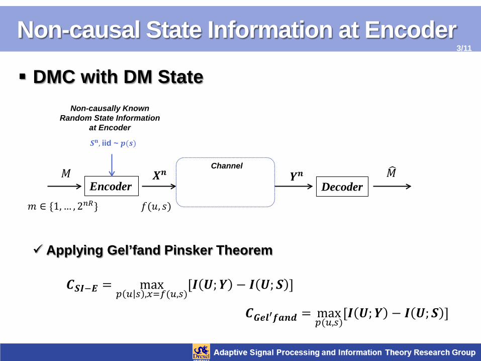
DMC with DM State
Applying Gel’fand Pinsker Theorem
Encoder Decoder
𝑺𝐧, iid ~ 𝒑(𝒔)
𝑀 𝒀𝒏 𝑀�
Non-causally Known Random State Information
at Encoder
Channel
𝑚 ∈ {1, … , 2𝑛𝑛}
𝑪𝑺𝑺−𝑬 = max𝑝 𝑢 𝑠 ,𝑥=𝑓(𝑢,𝑠)
[𝑺 𝑼;𝒀 − 𝑺 𝑼;𝑺 ]
𝑿𝒏
𝑪𝑮𝑮𝒍′𝒇𝒇𝒏𝒇 = max𝑝(𝑢,𝑠)
[𝑺 𝑼;𝒀 − 𝑺 𝑼;𝑺 ]
𝑓(𝑢, 𝑠)

Converse Proof
4/11
⋅ Let 𝑅 be an achievable rate, ∃ (2𝑛𝑛 ,𝑛) code with 𝑃𝑒 → 0 as 𝑛 → ∞.
⋅ Find the auxiliary random variable 𝑈𝑖 that forms
Markov Chain 𝑼𝒊 → 𝑿𝒊,𝑺𝒊 → 𝒀𝒊,
𝑛𝑅 = 𝐻(𝑀)
= 𝐻 𝑀 −𝐻 𝑀 𝑌𝑛 + 𝐻(𝑀|𝑌𝑛)
= 𝐼(𝑀;𝑌𝑛) + 𝐻(𝑀|𝑌𝑛) ← By Fano’s Iemma 𝐻 𝑀 𝑌𝑛 ≤ 𝑛 𝜖𝑛
≤ 𝐼 𝑀;𝑌𝑛 + 𝑛𝜖𝑛
= 𝐻 𝑌𝑛 − 𝐻 𝑌𝑛 𝑀 + 𝑛 𝜖𝑛
← +0
Converse Proof
5/11
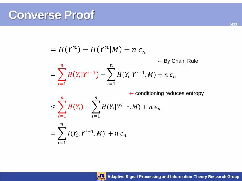
← By Chain Rule
= 𝐻 𝑌𝑛 − 𝐻 𝑌𝑛 𝑀 + 𝑛 𝜖𝑛
= �𝐻 𝑌𝑖|𝑌𝑖−1𝑛
𝑖=1
−�𝐻(𝑌𝑖|𝑌𝑖−1,𝑀)𝑛
𝑖=1
+ 𝑛 𝜖𝑛
≤�𝐻 𝑌𝑖
𝑛
𝑖=1
−�𝐻(𝑌𝑖|𝑌𝑖−1,𝑀)𝑛
𝑖=1
+ 𝑛 𝜖𝑛
← conditioning reduces entropy
= �𝐼(𝑌𝑖;𝑌𝑖−1,𝑀) 𝑛
𝑖=1
+ 𝑛 𝜖𝑛
Converse Proof
6/11
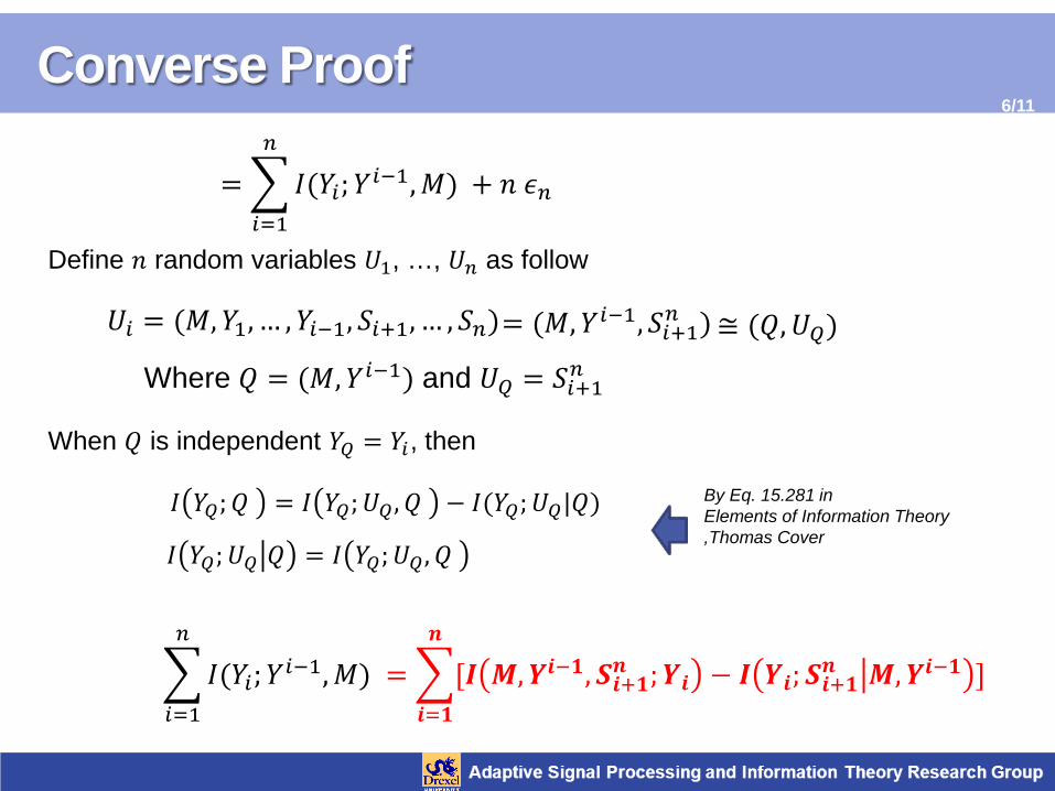
= �𝐼(𝑌𝑖;𝑌𝑖−1,𝑀) 𝑛
𝑖=1
+ 𝑛 𝜖𝑛
Define 𝑛 random variables 𝑈1, …, 𝑈𝑛 as follow
𝑈𝑖 = (𝑀,𝑌1, … ,𝑌𝑖−1, 𝑆𝑖+1, … , 𝑆𝑛) = (𝑀,𝑌𝑖−1, 𝑆𝑖+1𝑛 ) ≅ (𝑄,𝑈𝑄)
Where 𝑄 = (𝑀,𝑌𝑖−1) and 𝑈𝑄 = 𝑆𝑖+1𝑛
𝐼 𝑌𝑄;𝑄 = 𝐼 𝑌𝑄;𝑈𝑄,𝑄 − 𝐼(𝑌𝑄;𝑈𝑄|𝑄)
�𝐼(𝑌𝑖;𝑌𝑖−1,𝑀) 𝑛
𝑖=1
= �[𝑺 𝑴,𝒀𝒊−𝟏,𝑺𝒊+𝟏𝒏 ;𝒀𝒊 − 𝑺 𝒀𝒊;𝑺𝒊+𝟏𝒏 𝑴,𝒀𝒊−𝟏 ] 𝒏
𝒊=𝟏
When 𝑄 is independent 𝑌𝑄 = 𝑌𝑖, then
By Eq. 15.281 in Elements of Information Theory ,Thomas Cover
𝐼 𝑌𝑄;𝑈𝑄 𝑄 = 𝐼 𝑌𝑄;𝑈𝑄,𝑄
Converse Proof
7/11
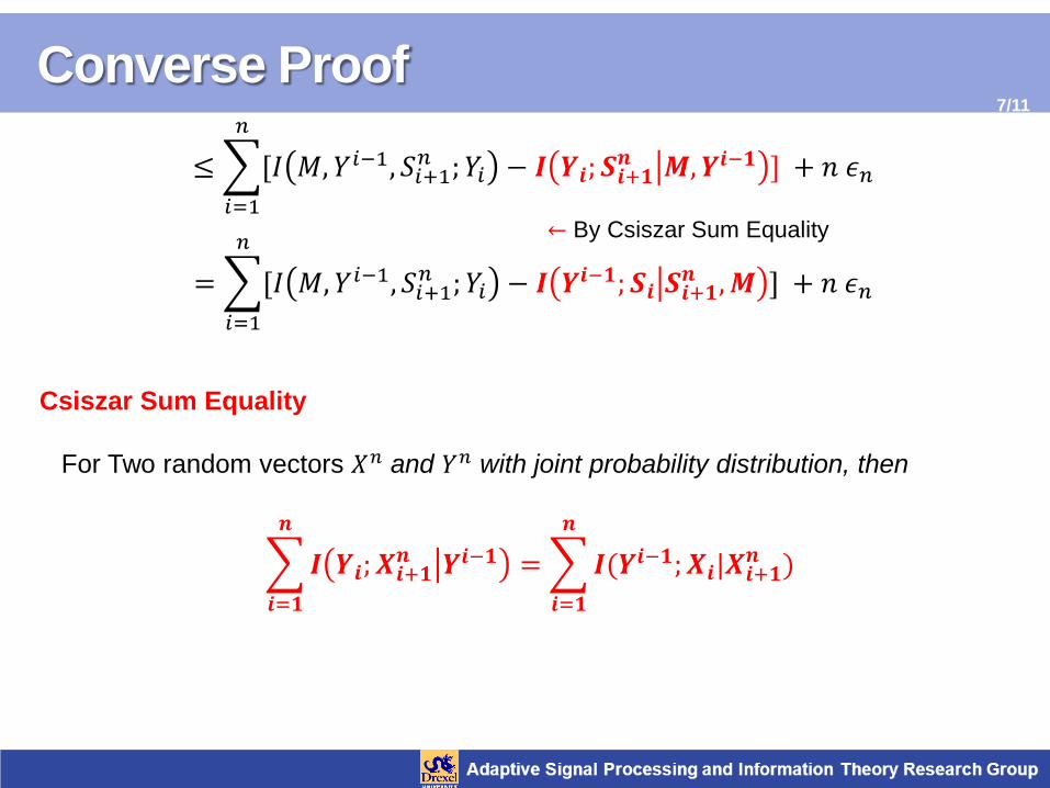
← By Csiszar Sum Equality
≤�[𝐼 𝑀,𝑌𝑖−1, 𝑆𝑖+1𝑛 ;𝑌𝑖 − 𝑺 𝒀𝒊;𝑺𝒊+𝟏𝒏 𝑴,𝒀𝒊−𝟏 ] 𝑛
𝑖=1
+ 𝑛 𝜖𝑛
= �[𝐼 𝑀,𝑌𝑖−1, 𝑆𝑖+1𝑛 ;𝑌𝑖 − 𝑺 𝒀𝒊−𝟏;𝑺𝒊 𝑺𝒊+𝟏𝒏 ,𝑴 ] 𝑛
𝑖=1
+ 𝑛 𝜖𝑛
�𝑺 𝒀𝒊;𝑿𝒊+𝟏𝒏 𝒀𝒊−𝟏𝒏
𝒊=𝟏
= �𝑺(𝒀𝒊−𝟏;𝑿𝒊|𝑿𝒊+𝟏𝒏 ) 𝒏
𝒊=𝟏
Csiszar Sum Equality For Two random vectors 𝑋𝑛 and 𝑌𝑛 with joint probability distribution, then
Csiszar Sum Equality Proof
8/11
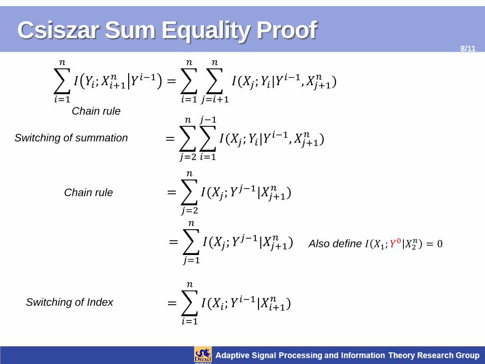
�𝐼 𝑌𝑖;𝑋𝑖+1𝑛 𝑌𝑖−1𝑛
𝑖=1
= � � 𝐼(𝑋𝑗;𝑌𝑖|𝑌𝑖−1,𝑋𝑗+1𝑛 ) 𝑛
𝑗=𝑖+1
𝑛
𝑖=1
= ��𝐼(𝑋𝑗;𝑌𝑖|𝑌𝑖−1,𝑋𝑗+1𝑛 ) 𝑗−1
𝑖=1
𝑛
𝑗=2
= �𝐼(𝑋𝑗;𝑌𝑗−1|𝑋𝑗+1𝑛 )𝑛
𝑗=2
= �𝐼(𝑋𝑗;𝑌𝑗−1|𝑋𝑗+1𝑛 )𝑛
𝑗=1
= �𝐼(𝑋𝑖;𝑌𝑖−1|𝑋𝑖+1𝑛 )𝑛
𝑖=1
Chain rule
Switching of summation
Chain rule
Also define 𝐼 𝑋1;𝑌0 𝑋2𝑛 = 0
Switching of Index
Converse Proof
9/11
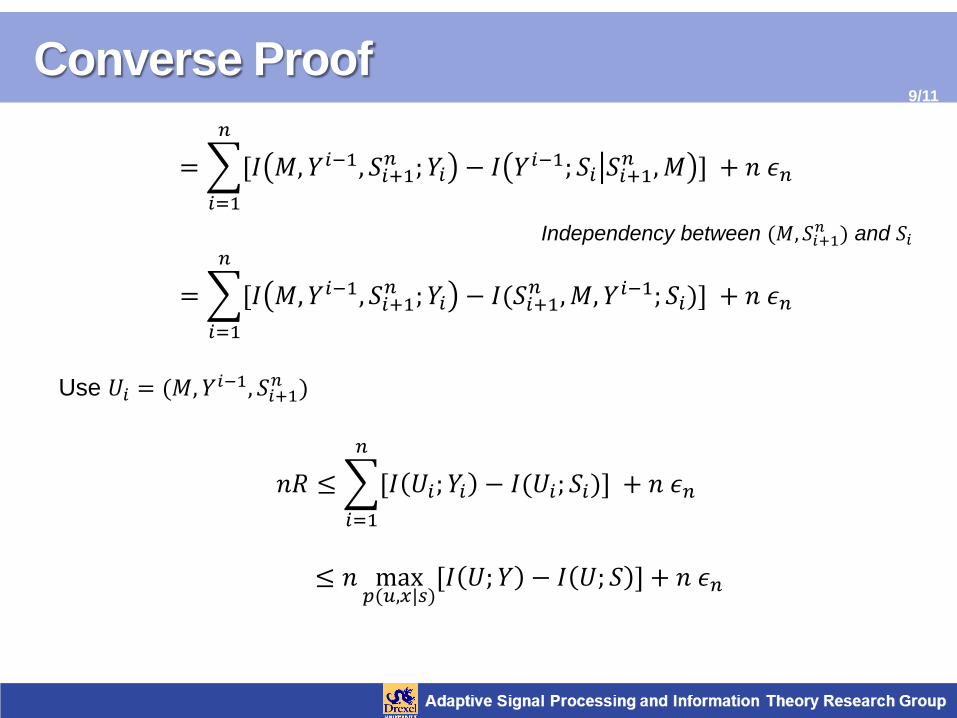
= �[𝐼 𝑀,𝑌𝑖−1, 𝑆𝑖+1𝑛 ;𝑌𝑖 − 𝐼 𝑌𝑖−1; 𝑆𝑖 𝑆𝑖+1𝑛 ,𝑀 ] 𝑛
𝑖=1
+ 𝑛 𝜖𝑛
= �[𝐼 𝑀,𝑌𝑖−1, 𝑆𝑖+1𝑛 ;𝑌𝑖 − 𝐼(𝑆𝑖+1𝑛 ,𝑀,𝑌𝑖−1; 𝑆𝑖)] 𝑛
𝑖=1
+ 𝑛 𝜖𝑛
Independency between (𝑀, 𝑆𝑖+1𝑛 ) and 𝑆𝑖
Use 𝑈𝑖 = (𝑀,𝑌𝑖−1, 𝑆𝑖+1𝑛 )
𝑛𝑅 ≤�[𝐼 𝑈𝑖;𝑌𝑖 − 𝐼(𝑈𝑖; 𝑆𝑖)] 𝑛
𝑖=1
+ 𝑛 𝜖𝑛
≤ 𝑛 max𝑝(𝑢,𝑥|𝑠)
[𝐼 𝑈;𝑌 − 𝐼 𝑈; 𝑆 ] + 𝑛 𝜖𝑛
Converse Proof
10/11
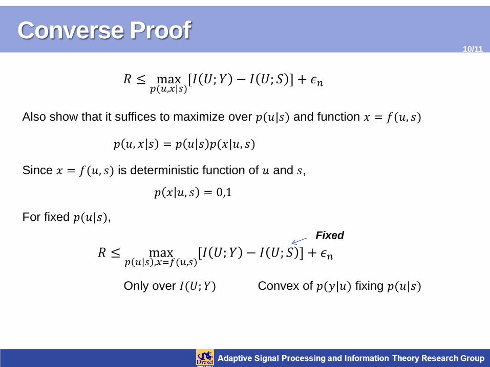
𝑅 ≤ max𝑝(𝑢,𝑥|𝑠)
[𝐼 𝑈;𝑌 − 𝐼 𝑈; 𝑆 ] + 𝜖𝑛
Also show that it suffices to maximize over 𝑝(𝑢|𝑠) and function 𝑥 = 𝑓(𝑢, 𝑠)
𝑝 𝑢, 𝑥 𝑠 = 𝑝 𝑢 𝑠 𝑝(𝑥|𝑢, 𝑠)
𝑝 𝑥 𝑢, 𝑠 = 0,1
Since 𝑥 = 𝑓(𝑢, 𝑠) is deterministic function of 𝑢 and 𝑠,
For fixed 𝑝(𝑢|𝑠),
𝑅 ≤ max𝑝 𝑢 𝑠 ,𝑥=𝑓(𝑢,𝑠)
[𝐼 𝑈;𝑌 − 𝐼 𝑈; 𝑆 ] + 𝜖𝑛 Fixed
Only over 𝐼(𝑈;𝑌) Convex of 𝑝(𝑦|𝑢) fixing 𝑝(𝑢|𝑠)
Converse Proof
11/11
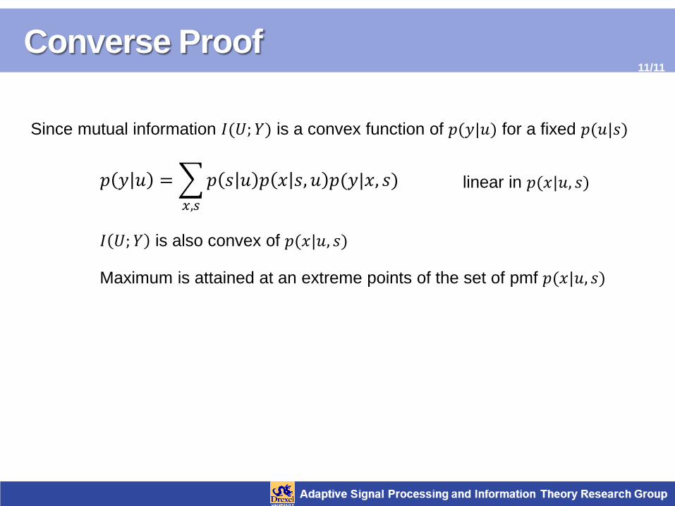
Since mutual information 𝐼(𝑈;𝑌) is a convex function of 𝑝(𝑦|𝑢) for a fixed 𝑝(𝑢|𝑠)
𝑝 𝑦 𝑢 = �𝑝 𝑠 𝑢 𝑝 𝑥 𝑠,𝑢 𝑝(𝑦|𝑥, 𝑠)𝑥,𝑠
linear in 𝑝(𝑥|𝑢, 𝑠)
𝐼 𝑈;𝑌 is also convex of 𝑝(𝑥|𝑢, 𝑠)
Maximum is attained at an extreme points of the set of pmf 𝑝(𝑥|𝑢, 𝑠)