DIRECTORATE OF DISTANCE EDUCATION · Unit-1:Introduction: Definition of Operating system-Computer...

ALAGAPPA UNIVERSITY (Accredited with ‘A+’ Grade by NAAC (with CGPA: 3.64) in the Third Cycle and

Graded as category - I University by MHRD-UGC)

(A State University Established by the Government of Tamilnadu)

KARAIKUDI – 630 003

DIRECTORATE OF DISTANCE EDUCATION

M.Sc. (INFORMATION TECHNOLOGY)

Second Year – Third Semester

31332–Operating Systems

Copy Right Reserved For Private Use only

Author:

Dr. K. Shankar

Assistant Professor

Department of Computer Science and Information Technology

Kalasalingam Academy of Research and Education

Anand Nagar, Krishnankoil-626126

“The Copyright shall be vested with Alagappa University”

All rights reserved. No part of this publication which is material protected by this copyright notice may be

reproduced or transmitted or utilized or stored in any form or by any means now known or hereinafter invented,

electronic, digital or mechanical, including photocopying, scanning, recording or by any information storage or

retrieval system, without prior written permission from the Alagappa University, Karaikudi, Tamil Nadu.

Reviwer:

Dr. P. Prabhu

Assistant Professor in Information Technology

Directorate of Distance Education

Alagappa University,

Karaikudi.

SYLLABI-BOOK MAPPING TABLE

Operating Systems

SYLLABI MAPPING IN BOOK

BLOCK1: INTRODUCTION

Unit-1:Introduction: Definition of Operating system-Computer System

Organization

Unit-2:Computer System Architecture: Operating System Structure-

Operating-System Operations

Unit-3:System Structures: Operating System Services- System Calls--

System Programs- Operating System Design and Implementation

Pages 1-12

Pages 13-24

Pages 25-43

BLOCK 2: PROCESS CONCEPT

Unit-4:Process Concept: Process Scheduling-Operations on Processes-

Inter process Communication

Unit-5:Process Scheduling: Scheduling concepts-Scheduling Criteria-

Scheduling Algorithms-Multiple Processor Scheduling

Pages 44-62

Pages 63-79

BLOCK 3: SYNCHRONIZATION

Unit-6:Synchronization:Semaphores-Classic Problems of

Synchronization-Monitors

Unit-7:Deadlocks: Deadlocks Characterization-Methods for Handling

Deadlocks

Unit-8: Deadlock Prevention-Avoidance-Detection-Recovery from

Deadlock

Pages 80-104

Pages 105-112

Pages 113-132

BLOCK 4: MEMORY MANAGEMENT

Unit-9:Memory Management Strategies: Swapping-Contiguous

Memory Allocation- Paging- Segmentatio

Pages 133-160

BLOCK 5: FILE SYSTEM

Unit-10: File Concept: Access Methods-Directory

Unit-11: Structure: File System Monitoring-File Sharing-Protection

Unit-12: Implementing File Systems: File System Structure-File

System Implementation

Unit-13: Directory Implementation: Allocation Methods-Free Space

Management

Unit-14: Secondary Storage Structure: Overview of Mass-Storage

Structure-Disk Structure-Disk Attachment-Disk Scheduling-Disk

Management

Model Question Paper

Pages 161-173

Pages 174-186

Pages 187-196

Pages 197-207

Pages 208-225

Pages 226-227

CONTENTS

BLOCK1: INTRODUCTION

UNIT 1: INTRODUCTION 1-12

1.0 Introduction

1.1Objective

1.2 Operating System

1.2.1 User View

1.2.2 System View

1.3 Definition of Operating system

1.4 Computer System Organization

1.4.1 Computer System Operation

1.4.2 Storage Structure

1.4.3 I/O Structure

1.5 Answers to Check Your Progress Questions

1.6 Summary

1.7 Key Words

1.8 Self Assessment Questions and Exercises

1.9 Further Readings

UNIT 2 COMPUTER SYSTEM ARCHITECTURE 13-24

2.0 Introduction

2.1 Objective

2.2 Computer-System Architecture

2.2.1 Multiprocessor structures or Parallel Systems

2.2.2 Desktop Systems

2.2.3 The Multi programmed systems

2.2.4 Time-Sharing Systems–Interactive Computing

2.2.5 Distributed Systems

2.2.6 Client server systems

2.2.7 Peer to Peer System

2.2.8 Clustered Systems

2.2.9 Real-Time Systems

2.3 Operating-System Operations

2.3.1 Dual-Mode and Multimode Operation

2.3.2 Timer


2.5 Summary

2.6 Key Words



UNIT 3 SYSTEM STRUCTURES 25-43

3.0 Introduction

3.1 Objective

3.2 Operating-System Structure

3.2.1 Simple Structure

3.2.2 Layered Approach

3.3.3 Microkernels

3.3.4 Modules

3.3.5 Hybrid Systems

3.3.6 Mac OS X

3.3.7 iOS

3.3.8 Android

3.4 Operating System Services

3.5. System Calls

3.5.1 Types of System Calls

3.6 System Programs

3.7 Operating-System Design and Implementation


3.9 Summary

3.10 Key Words



BLOCK II: PROCESS CONCEPT

UNIT 4 : PROCESS CONCEPT 44-62

4.0 Introduction

4.1 Objective

4.2 Process Concept

4.2.1The Process

4.2.2 Process State

4.2.3 Process Control Block

4.2.4Threads

4.3 Process Scheduling

4.4Operations on Processes

4.4.1 Process Creation

4.4.2 Process Termination

4.5 Inter process Communication

4.5.1 Shared-Memory Systems

4.5.2 Message-Passing Systems

4.5.2.1 Naming

4.5.2.2 Synchronization

4.5.2.3 Buffering


4.7 Summary

4.8 Key Words



UNIT 5: PROCESS SCHEDULING 63-79

5.0 Introduction

5.1 Objective


5.2.1 Scheduling concepts

5.3 Scheduling Criteria

5.4Scheduling Algorithms

5.4.1First-Come, First-Served Scheduling

5.4.2 Shortest-Job-First Scheduling

5.4.3 Priority Scheduling

5.4.4 Round-Robin Scheduling

5.4.5 Multilevel Queue Scheduling

5.4.6 Multilevel Feedback Queue Scheduling

5.4.7 Thread Scheduling

5.4.8 Pthread Scheduling

5.5 Multiple-Processor Scheduling

5.5.1 Approaches to Multiple-Processor Scheduling

5.5.2 Processor Affinity

5.5.3 Load Balancing

5.5.4 Multicore Processors


5.7 Summary

5.8 Key Words



BLOCK III: SYNCHRONIZATION

UNIT 6 : SYNCHRONIZATION 80-104

6.0Introduction

6.1 Objective

6.2 The Critical-Section Problem

6.3 Synchronization Hardware

6.4 Semaphores

6.4.1 Semaphore Usage

6.4.2 Semaphore Implementation

6.5 Semaphores -Classic Problems of Synchronization

6.5.1 The Bounded-Buffer Problem

6.5.2 The Readers–Writers Problem

6.5.3 The Dining-Philosophers Problem

6.6 Semaphores -Classic Problems of Synchronization -Monitors

6.6.1 Monitor Usage

6.6.2 Dining-Philosophers Solution Using Monitors

6.6.3 Implementing a Monitor Using Semaphores

6.6.4 Resuming Processes within a Monitor


6.8 Summary

6.9 Key Words



UNIT 7: DEADLOCK 105-112

7.0Introduction

7.1 Objective

7.2 Deadlock Characterization

7.2.1 Resource-Allocation Graph

7.3 Methods Handing Deadlocks


7.5 Summary

7.6 Key Words



UNIT 8 : DEADLOCK PREVENTION 113-132

8.0 Introduction

8.1 Objective

8.2 Deadlock Prevention

8.2.1 Mutual Exclusion

8.2.2 Hold and Wait

8.2.3 No Pre-emption

8.2.4 Circular Wait

8.3 Deadlock Avoidance

8.3.1 Safe State

8.3.2 Resource-Allocation-Graph Algorithm

8.3.3 Banker’s Algorithm

8.3.4 Safety Algorithm

8.3.5 Resource-Request Algorithm

8.3.6 An Illustrative Example

8.4 Deadlock Detection

8.4.1 Single Instance of Each Resource Type

8.4.2 Several Instances of a Resource Type

8.4.3 Detection-Algorithm Usage

8.5 Recovery from Deadlock


8.5.2 Resource Pre-emption


8.7 Summary

8.8 Key Words



BLOCK 4: MEMORY MANAGEMENT

UNIT 9 : MEMORY MANAGEMENT STRATEGIES 133-160

9.0 Introduction

9.1 Objective

9.2 Swapping

9.2.1 Standard Swapping

9.2.2 Swapping on Mobile Systems

9.3 Swapping-Contiguous Memory Allocation- Paging- Segmentation

9.3.1 Memory Protection

9.3.2 Memory Allocation

9.3.3 Fragmentation

9.4 Paging

9.4.1 Basic Method

9.4.2 Hardware Support

9.4.3 Protection

9.4.4 Shared Pages

9.4.5 Hierarchical Paging

9.4.6 Hashed Page Tables

9.4.7 Inverted Page Tables

9.5 Segmentation

9.5.1 Basic Method

9.5.2 Segmentation Hardware


9.7 Summary

9.8 Key Words



BLOCK 5: FILE SYSTEM

UNITS 10 FILE CONCEPT 161-173

10.0 Introduction

10.1 Objectives

10.2 File Concept

10.2.1 File Attributes

10.2.2 File Operations

10.3 Access Methods

10.3.1 Sequential Access

10.3.2 Direct Access

10.3.3 Other Access Methods

10.4 Directory Overview

10.4.1 Single-Level Directory

10.4.2 Two-Level Directory

10.4.3Tree-Structured Directories

10.4.4 Acyclic-Graph Directories

10.4.5General Graph Directory


10.6 Summary

10.7 Key Words



UNIT 11 STRUCTURES 174-186

11.0 Introduction

11.1Objective

11.2 File-System Mounting

11.3 File Sharing

11.3.1 Multiple Users

11.3.2 Remote File Systems

11.3.3 The Client–Server Model

11.3.4 Distributed Information Systems

11.3.5 Failure Modes

11.3.6 Consistency Semantics

11.3.7 Immutable-Shared-Files Semantics

11.4 Protection

11.4.1 Types of Access

11.4.2 Access Control


11.6 Summary

11.7 Key Words



UNIT 12 IMPLEMENTING FILE SYSTEMS 187-196

12.0 Introduction

12.1 Objectives

12.2 File-System Structure

12.3 File-System Implementation

12.3.1 Overview

12.3.2 Partitions and Mounting

12.3.3 Virtual File Systems


12.5 Summary

12.6 Key Words



UNIT 13 DIRECTORY IMPLEMENTATION 197-208

13.0 Introduction

13.1 Objective

13.2 Directory Implementation

13.2.1 Linear List

13.2.1 Hash Table

13.3 Allocation Methods

13.3.1 Contiguous Allocation

13.3.2 Linked Allocation

13.3.3 Indexed Allocation

13.4 Free-Space Management

13.4.1 Bit Vector

13.4.2 Linked List

13.4.3 Grouping

13.4.4 Counting

13.4.5 Space Maps


13.6 Summary

13.7 Key Words



UNIT 14 SECONDARY STORAGE STRUCTURE 209-225

14.0Introduction

14.1Objective

14.2 Overview of Mass-Storage Structure

14.2.1 Magnetic Disks

14.2.2 Solid-State Disks

14.2.3 Magnetic Tapes

14.2.4 Disk Transfer Rates

14.3 Disk Structure

14.4 Disk Attachment

14.4.1 Host-Attached Storage

14.4.2 Network-Attached Storage

14.4.3 Storage-Area Network

14.5 Overview of Mass-Storage Structure-Disk Attachment-Disk Scheduling-Disk

Management

14.5.1 FCFS Scheduling

14.5.2 SSTF Scheduling

14.5.3 SCAN Scheduling

14.5.4 C-SCAN Scheduling

14.5.5 LOOK Scheduling

14.5.6 Selection of a Disk-Scheduling Algorithm

14.6 Disk Management

14.6.1 Disk Formatting

14.6.2 Boot Block

14.6.3 Bad Blocks


14.8 Summary

14.9 Key Words



MODEL QUESTION PAPER 226-227

1

Introduction

Notes

Self – Instructional Material

BLOCK – I INTRODUCTION

UNIT 1 INTRODUCTION

Structure

1.0 Introduction

1.1 Objective

1.2 Operating System

1.3 Definition of Operating system

1.4 Computer System Organization

1.5 Check Your Progress


1.7 Summary

1.8 Key Words

1.9 Self-Assessment Questions and Exercises


1.0 INTRODUCTION

Operating system is the interface between the hardware and software. The

purpose of an operating system is to provide an environment in which a

user can execute programs in a convenient and efficient manner. An

operating system is a software that manages the computer hardware. The

hardware must provide appropriate mechanisms to ensure the correct

operation of the computer system and to prevent user programs from

interfering with the proper operation of the system. This unit covers the

basics of operating system and how the entire computer system is

organized. Definition of Operating System can be defined as,

An operating system is a program that controls the execution of

application programs and acts as an interface between the user of a

computer and the computer hardware.

A more common definition is that the operating system is the one

program running at all times on the computer (usually called the

kernel), with all else being application programs.

An operating system is concerned with the allocation of resources

and services, such as memory, processors, devices, and

information. The operating system correspondingly includes

programs to manage these resources, such as a traffic controller, a

scheduler, memory management module, I/O programs, and a file

system.

1.1 OBJECTIVE

This not helps the user to

Understand operating system

2

Introduction

Notes


Learn different computer system organization

1.2 OPERATING SYSTEM

computer system can be divided roughly into four components: the

hardware, the operating system, the software programs, and the users. The

hardware—the central processing unit (CPU), the memory, and the

input/output (I/O) devices—provide the simple computing sources for the

system. The software programs—such as phrase processors, spreadsheets,

compilers, and Web browsers—define the methods in which these assets

are used to remedy users’ computing problems. The running gadget

controls the hardware and coordinates its use amongst the variety of utility

programs for the variety of users. In view a laptop device as consisting of

hardware, software program and data. The operating gadget offers the

means for appropriate use of these assets in the operation of the pc system.

An operating system is comparable to a government. Like a government, it

performs no useful feature by way of itself. It truly gives an environment

inside which other programs can do beneficial work.

1.2.1 User View

The user’s view of the laptop varies according to the interface being used.

Most laptop customers take a seat in the front of a PC, consisting of a

monitor, keyboard, mouse, and system unit. Such a gadget is designed for

one user. The purpose is to maximize the work (or play) that the user is

performing. In this case, the operating system is designed mostly for ease

of use, with some interest paid to overall performance and none paid to

resource utilization—how more than a few hardware and software program

sources are shared. Performance is, of course, necessary to the user;

3

Introduction

Notes


however, such systems are optimized for the single-user trip as a substitute

than the necessities of multiple users. In other cases, a user sits at a

terminal related to a mainframe or a minicomputer. Other customers are

having access to the same laptop through different terminals. These

customers share sources and can also trade information.

The working machine in such cases is designed to maximize aid

utilization— to guarantee that all handy CPU time, memory, and I/O are

used efficiently and that no man or woman person takes greater than her

truthful share. In still other cases, customers sit down at workstations

related to networks of different workstations and servers. These customers

have dedicated resources at their disposal; however, they additionally share

sources such as networking and servers, such as file, compute, and print

servers. Therefore, their running machine is designed to compromise

between person usability and useful resource utilization.

Recently, many types of mobile computers, such as smartphones and

tablets, have come into fashion. Most mobile computers are standalone

gadgets for individual users. Quite often, they are related to networks

through mobile or other Wi-Fi technologies. Increasingly, these cell

devices are replacing computer and laptop computers for human beings

who are exceptionally interested in the usage of computers for electronic

mail and web browsing. The user interface for cellular computer systems

normally aspects a touch screen, the place the person interacts with the

device with the aid of pressing and swiping fingers throughout the display

as an alternative than using a physical keyboard and mouse. Some

computers have little or no user view. For example, embedded computers

in home units and cars may additionally have numeric keypads and might

also turn indicator lights on or off to show status, however they and their

running structures are designed notably to run without user intervention

1.2.2 System View

From the computer’s point of view, the operating device is the application

most intimately worried with the hardware. In this context, we can view an

operating device as a resource allocator. A computer device has many

resources that may be required to remedy a problem: CPU time,

reminiscence space, file-storage space, I/O devices, and so on. The running

system acts as the manager of these resources. Facing numerous and

maybe conflicting requests for resources, the operating device ought to

figure out how to allocate them to precise applications and users so that it

can operate the laptop machine effectively and fairly. As the, aid allocation

is especially important where many users access the identical mainframe or

minicomputer. A barely special view of an operating system emphasizes

the need to control the range of I/O devices and user programs. An

operating system is a manipulate program. A manage software manages

the execution of user programs to forestall errors and unsuitable use of the

computer. It is especially worried with the operation and manages of I/O

device.

4

Introduction

Notes


1.3 DEFINITION OF OPERATING SYSTEM

A set of software that controls the ordinary operation of a laptop system,

generally through performing such tasks as reminiscence allocation, job

scheduling, and input/output control. A running machine is a program that

manages the laptop hardware. It also offers a basis for software

applications and acts as an intermediary between the laptop person and the

laptop hardware. An operating system acts as an intermediary between the

consumer of the computer and computer hardware. The cause of a working

gadget is to grant surroundings in which a person can execute applications

in a convenient and efficient manner.

An operating machine is software program that manages the computer

hardware. The hardware has to provide appropriate mechanisms to ensure

the correct operation of laptop gadget and to prevent user applications from

interfering with proper operation of the system.

Fig 1.2 working of Operating System

In addition, we have no universally generic definition of what is section of

the running system. A simple viewpoint is that it includes the whole thing a

seller ships when you order ―the running system.‖ The facets included,

however, fluctuate significantly across systems. Some systems take up

much less than a megabyte of space and lack even a full-screen editor,

whereas others require gigabytes of space and are based entirely on

graphical windowing systems. A greater common definition, and the one

that we generally follow, is that the working machine is the one application

walking at all instances on the computer—usually called the kernel.

Along with the kernel, there are two other types of programs: system

programs, which are related with the operating device but are now not

necessarily phase of the kernel, and application programs, which consist of

all programs now not associated with the operation of the system. The

matter of what constitutes a working device grew to be increasingly

necessary as personal computer systems grew to be greater extensive and

working structures grew increasingly more sophisticated. In 1998, the

United States Department of Justice filed go well with against Microsoft,

5

Introduction

Notes


in essence claiming that Microsoft blanketed too plenty functionality in its

running structures and consequently avoided application companies from

competing.

For example, a Web browser was a necessary phase of the working

systems. As a result, Microsoft was once determined guilty of the use of its

operating-system monopoly to limit competition. Today, however, if we

seem to be at running systems for cellular devices, we see that once again

the variety of features constituting the running gadget

1.4 COMPUTER SYSTEM ORGANIZATION

1.4.1 Computer System Operation

A modern-day general-purpose computer gadget consists of one or extra

CPUs and a quantity of machine controllers connected via a frequent bus

that presents get right of entry to shared memory. Each device controller is

in charge of a particular type of machine (for example, disk drives, audio

devices, or video displays). The CPU and the system controllers can

execute in parallel, competing for reminiscence cycles. To make certain

orderly get entry to the shared memory, a reminiscence controller

synchronizes get entry to the memory.

Figure 1.3 modernized computer system

There are numerous elements however three of them are main components

in a pc system. They are the Central Processing Unit (CPU), reMemory

(RAM and ROM) and Input, Output devices. The CPU is the predominant

unit that technique data. Memory holds records required for processing.

The input and output devices allow the customers to communicate with the

computer.

The mechanism for every of the components to talk with every different is

the bus architecture. It is a digital verbal exchange system, which includes

information via electronic pathways known as circuit lines. The gadget bus

is divided into three kinds referred to as tackle bus, facts bus and

manipulates bus.

6

Introduction

Notes


Figure 1.4 Timeline of Interrupts

Once the kernel is loaded and executing, it can begin offering services to

the machine and its users. Some services are supplied outside of the kernel,

through device programs that are loaded into memory at boot time to come

to be gadget processes, or system daemons that run the entire time the

kernel is running. On UNIX, the first machine method is ―init,‖ and it

begins many other daemons. Once this phase is complete, the system is

entirely booted, and the device waits for some event to occur. The

prevalence of a tournament is generally signaled through an interrupt from

both the hardware or the software. Hardware might also set off an interrupt

at any time via sending a signal to the CPU, normally by using way of the

device bus. Software may additionally set off an interrupt via executing a

one-of-a-kind operation called a system call (also called a display call).

When the CPU is interrupted, it stops what it is doing and right away

transfers execution to a constant location. The constant place typically

contains the beginning tackle the place the service movements for the

interrupt is located. The interrupt service hobby executes; on completion,

the CPU resumes the interrupted computation. A timeline of this operation

is proven in Figure 1.4. Interrupts are a necessary section of pc

architecture. Each laptop graph has its own interrupt mechanism, but a

number of features are common. The interrupt should switch and

manipulate to the excellent interrupt carrier routine. The easy approach for

handling this switch would be to invoke usual pursuits to examine the

interrupt information. The routine, in turn, would call the interrupt-specific

handler.

However, interrupts need to be treated quickly. Since only a predefined

number of interrupts is possible, a desk of pointers to interrupt routines can

be used as an alternative to provide the vital speed. The interrupt

movement is known as indirectly through the table, with no intermediate

hobbies needed. Generally, the desk of pointers is stored in low

reminiscence (the first hundred or so locations). These areas preserve the

addresses of the interrupt carrier routines for the number devices. This

array, or interrupt vector, of addresses is then listed via a unique machine

number, given with the interrupt request, to grant the address of the

interrupt service routine for the interrupting device. Operating systems as

different as Windows and UNIX dispatch interrupts in this manner.

7

Introduction

Notes


The interrupt structure must additionally retailer the address of the

interrupted instruction. Many historical designs truly stored the interrupt

tackle in a fixed place or in a location listed by way of the gadget number.

More current architectures save the return address on the system stack. If

the interrupt activities wish to regulate the processor state—for instance,

through modifying register values—it has to explicitly shop the modern-

day kingdom and then restore that nation earlier than returning. After the

interrupt is serviced, the saved return address is loaded into the program

counter, and the interrupted computation resumes as even though the

interrupt had not occurred.

1.4.2 Storage Structure

The CPU can load instructions only from memory, so any packages to run

have to be stored there. General-purpose computer systems run most of

their programs from rewritable memory, referred to as principal memory

(also called random-access memory, or RAM). Main reminiscence

frequently is implemented in a semiconductor science known as dynamic

random-access reminiscence (DRAM). Computers use other forms of

memory as well. We have already stated read-only memory, ROM) and

electrically erasable programmable read-only memory, EEPROM).

Because ROM can't be changed, solely static programs, such as the

bootstrap application described earlier, are stored there.

The immutability of ROM is of use in game cartridges. EEPROM can be

changed however cannot be changed frequently and so carries often static

programs. For example, smartphones have EEPROM to keep their factory-

installed programs. All forms of reminiscence grant an array of bytes. Each

byte has its personal address. Interaction is achieved via a sequence of load

or store instructions to unique memory addresses. The load training moves

a byte or word from most important reminiscence to an inner register

inside the CPU, whereas the keep instruction moves the content material of

a register to primary memory. Aside from explicit hundreds and stores, the

CPU automatically masses directions from principal memory for

execution.

A regular instruction–execution cycle, as executed on a machine with von

Neumann architecture, first fetches an instruction from reminiscence and

shops that instruction in the coaching register. The coaching is then

decoded and can also cause operands to be fetched from reminiscence and

stored in some internal register. After the coaching on the operands has

been executed, the end result may also be saved lower back in memory.

Notice that the memory unit sees solely a flow of memory addresses. It

does not comprehend how they are generated (by the guidance counter,

indexing, indirection, literal addresses, or some different means) or what

they are for (instructions or data).

8

Introduction

Notes


Figure 1.5 Hierarchy of Storage Device

Accordingly, we can omit how a reminiscence address is generated

through a program. We are involved only in the sequence of memory

addresses generated by way of the going for walks program. Ideally, we

prefer the applications and facts to reside in major memory permanently.

This association usually is not feasible for the following two reasons: 1.

Main reminiscence is commonly too small to shop all needed programs

and records permanently.2. Main memory is an unstable storage system

that loses its contents when energy is turned off or otherwise lost. Thus,

most pc systems supply secondary storage as an extension of important

memory. The principal requirement for secondary storage is that it be able

to maintain large portions of statistics permanently. The most frequent

secondary-storage machine is a magnetic disk, which affords storage for

both packages and data. Most programs (system and application) are stored

on a disk until they are loaded into memory. Many programs then use the

Hence, the applicable management of disk storage is of central importance

to a pc system, as we talk about in. In a larger sense, however, the storage

shape that we have described current of registers, principal memory, and

magnetic disks—is only one of many possible storage systems. Others

consist of cache memory, CD-ROM, magnetic tapes, and so on. Each

storage system affords the simple functions of storing a datum and keeping

that datum until it is retrieved at a later time. The most important variations

among the various storage structures lie in speed, cost, size, and Volatility.

The huge range of storage structures can be organized in a hierarchy

(Figure 1.4) in accordance to speed and cost. The higher stages are

expensive; however, they are fast. As we move down the hierarchy, the

price per bit usually decreases, whereas the get right of entry to time

commonly increases. This trade-off is reasonable; if a given storage

machine have been each quicker and much less luxurious than another—

other homes being the same—then there would be no motive to use the

slower, extra high priced memory.

9

Introduction

Notes


In fact, many early storage devices, which includes paper tape and core

memories, are relegated to museums now that magnetic tape and

semiconductor memory have end up faster and cheaper. The top 4 degrees

of memory in Figure 1.4 can also be constructed the use of semiconductor

memory. In addition to differing in velocity and cost, a range of storage

systems are both unstable or nonvolatile. As stated earlier, unstable storage

loses its contents when the energy to the gadget is removed. In the absence

of highly-priced battery and generator backup systems, statistics must be

written to non-volatile storage for safekeeping.

The storage systems above the solid-state disk are volatile, whereas these

which includes the solid-state disk and under are nonvolatile. Solid-state

disks have countless editions but in regularly occurring are quicker than

magnetic disks and are nonvolatile. One type of solid-state disk stores

information in a large DRAM array during everyday operation however

also contains a hidden magnetic difficult disk and a battery for backup

power. If exterior strength is interrupted, this solid-state disk’s controller

copies the facts from RAM to the magnetic disk.

When exterior strength is restored, the controller copies the facts lower

back into RAM. Another form of solid-state disk is flash memory, which is

popular in cameras and private digital assistants (PDAs), in robots, and

increasingly more for storage on general-purpose computers. Flash

memory is slower than DRAM however needs no strength to retain its

contents. Another structure of nonvolatile storage is NVRAM, which is

DRAM with battery backup power. This memory can be as fast as DRAM

and (as lengthy as the battery lasts) is nonvolatile. The sketch of a whole

reminiscence gadget needs to stability all the elements just discussed: it

have to use solely as lots pricey memory as crucial whilst presenting as an

awful lot inexpensive, nonvolatile memory as possible. Caches can be

established to enhance overall performance where a massive disparity in

get right of entry to time or transfer fee exists between two components.

1.4.3 I/O Structure

Storage is solely one of many kinds of I/O gadgets within a computer. A

large element of working device code is committed to managing I/O, each

because of its importance to the reliability and overall performance of a

gadget and due to the fact of the various nature of the devices. Next, we

grant an overview of I/O. A general-purpose pc device consists of CPUs

and a couple of system controllers that are connected through a common

bus. Each machine controller is in cost of a precise kind of device.

Depending on the controller, more than one device may also be attached.

For instance, seven or more units can be attached to the small computer-

systems interface (SCSI) controller. A gadget controller continues some

local buffer storage and a set of special-purpose registers. The gadget

controller is accountable for moving the records between the peripheral

units that it controls and its nearby buffer storage.

Typically, working structures have a machine driver for every gadget

controller. This machine driver is familiar with the machine controller and

10

Introduction

Notes


provides the rest of the running system with a uniform interface to the

device. To begin an I/O operation, the gadget driver masses the appropriate

registers within the device controller. The gadget controller, in turn,

examines the contents of these registers to determine what action to take

(such as ―read a personality from the keyboard‖). The controller starts off

evolved the transfer of records from the machine to its nearby buffer. Once

the switch of statistics is complete, the system controller informs the

gadget driver via an interrupt that it has finished its operation. The device

driver then returns control to the running system, possibly returning the

statistics or a pointer to the facts if the operation was once a read. For other

operations, the system driver returns repute information. This form of

interrupt-driven I/O is great for transferring small amounts of data but can

produce high overhead when used for bulk data motion such as disk I/O.

To remedy this problem, direct reminiscence get right of entry to (DMA) is

used. After placing up buffers, pointers, and counters for the I/O device,

the gadget controller transfers a whole block of information immediately to

or from its very own buffer storage to memory, with no intervention by the

CPU. Only one interrupt is generated per block, to inform the device driver

that the operation has completed, as a substitute than the one interrupt per

byte generated for low-speed devices. While the system controller is

performing these operations, the CPU is reachable to accomplish other

work. Some high-end structures use switch as an alternative than bus

architecture. On these systems, multiple factors can discuss to different

factors concurrently, instead than competing for cycles on a shared bus. In

this case, DMA is even more effective. Figure 1.6 suggests the interplay of

all factors of a laptop system.

Check your Progress

1. What is an operating system?

2. What is the kernel?

3. What are the various components of a computer system?

4. What are the types of ROM?

5. What is SCSI?

1.5. ANSWERS TO CHECK YOUR PROGRESS

1. An operating system is a program that manages the computer

hardware. it acts as an intermediate between a user’s of a computer

and the computer hardware. It controls and coordinates the use of

the hardware among the various application programs for the

various users.

2. A more common definition is that the OS is the one program

running at all times on the computer, usually called the kernel, with

all else being application programs.

11

Introduction

Notes


3. A computer system can be divided roughly into four components:

the hardware, the operating system, the software programs, and the

users.

4. There are five basic ROM types:

ROM.

PROM.

EPROM.

EEPROM.

Flash memory

5. SCSI - Small computer systems interface is a type of interface used

for computer components such as hard drives, optical drives,

scanners and tape drives. It is a competing technology to standard

IDE (Integrated Drive Electronics).

1.6. SUMMARY

A computer system can be divided roughly into four components:

the hardware, the operating system, the software programs, and the

users.

An operating system is a program that controls the execution of

application programs and acts as an interface between the user of a

computer and the computer hardware.

When the CPU is interrupted, it stops what it is doing and right

away transfers execution to a constant location.

To begin an I/O operation, the gadget driver masses the appropriate

registers within the device controller.

Flash memory is slower than DRAM however needs no strength to

retain its contents.

The CPU can load instructions only from memory, so any packages

to run have to be stored there.

1.7. KEYWORDS

Operating system: An operating machine is software program that

manages the computer hardware.

Storage system: The storage systems above the solid-state disk are

volatile, whereas these which includes the solid-state disk and under

are nonvolatile.

Interrupt: Interrupt is the mechanism by which modules like I/O or

memory may interrupt the normal processing by CPU.

1.8. SELF ASSESSMENT QUESTIONS AND EXERCISES

Short Answer questions:

1. Explain the concept of the batched operating systems?

12

Introduction

Notes


2. What is purpose of different operating systems?

3. Difference between User View and System View?

4. Define I/O Structure?

5. Define Storage Structure?

Long Answer questions:

1. Explain Hierarchy of Storage Device?

2. Define Operating System and his working?

3. Define Computer System Organization?

1.9. FURTHER READINGS

Silberschatz, A., Galvin, P.B. and Gagne, G., 2006. Operating system

principles. John Wiley & Sons.

Tanenbaum, A.S. and Woodhull, A.S., 1997. Operating systems: design

and implementation (Vol. 68). Englewood Cliffs: Prentice Hall.

Deitel, H.M., Deitel, P.J. and Choffnes, D.R., 2004. Operating systems.

Delhi.: Pearson Education: Dorling Kindersley.

Stallings, W., 2012. Operating systems: internals and design principles.

Boston: Prentice Hall,.

13

Computer System

Architecture

Notes


UNIT II COMPUTER SYSTEM ARCHITECTURE

Structure 2.0 Introduction

2.1 Objective

2.2 Computer-System Architecture


2.4 Check Your Progress


2.6 Summary

2.7 Key Words

2.8 Self-Assessment Questions and Exercises


2.0 INTRODUCTION

This unit explains the structure of the operating system and the operations

associated with it. Computer architecture is a set of rules and methods that

describe the functionality, organization, and implementation of computer

systems. Some definitions of architecture define it as describing the

capabilities and programming model of a computer but not a particular

implementation. In other definitions computer architecture involves

instruction set architecture design, microarchitecture design, logic design,

and implementation. The structure of the system and the various types are

explained briefly. The different types of computer architecture and its

working are explained clearly.

2.1 OBJECTIVE

This unit helps the user to

Understand the various computer architecture

Learn the operations of operating system

2.2 COMPUTER-SYSTEM ARCHITECTURE

The laptop machine can be defined under many classes which are listed out

one with the aid of one below.

2.2.1 Multiprocessor structures or Parallel Systems

Multiprocessor systems with more than one CPU in close communication.

Tightly coupled machine – processors share reminiscence and a clock;

conversation typically takes location thru the shared memory. Although

single-processor systems are most common, multiprocessor structures (also

known as parallel systems or tightly coupled systems) are growing in

14

Computer System

Architecture

Notes


importance. Such structures have two or more processors in close

communication, sharing the pc bus and every now and then the clock,

memory, and peripheral devices.

Advantages of parallel system:

Increased throughput- By increasing the no of processors, work is

accomplished in less time.

Economical – multiprocessor system can shop more money because

they can share peripheral, mass storage and power supply.

Increased reliability- If one processor fields then the last processors

will share the work of the failed processors.

This is acknowledged as graceful degradation or fault tolerant

1. Increased throughput. By growing the quantity of

processors, we count on to get more work performed in less time.

2. Economy of scale.

3. Increased reliability.

The ability to continue offering provider proportional to the stage

of surviving hardware is called graceful degradation. Some

structures go past swish degradation and are referred to as fault

tolerant, because they can go through a failure of any single

component and nevertheless continue operation.

• The multiple-processor structures in use today are of two

types.

• Some structures use asymmetric multiprocessing, in which

every processor is assigned a particular task.

A master processor controls the system; the other processors both

appear to the master for instruction or have predefined tasks. This

scheme defines a master-slave relationship. The grasp processor

schedules and allocates work to the slave processors. The most

frequent structures use symmetric multiprocessing (SMP), in which

each processor performs all duties within the working system. SMP

capacity that all processors are peers; no master-slave relationship

exists between processors.

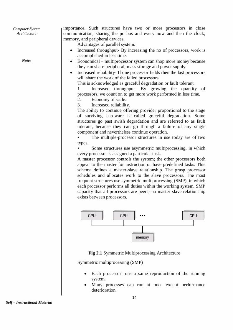
Fig 2.1 Symmetric Multiprocessing Architecture

Symmetric multiprocessing (SMP)

Each processor runs a same reproduction of the running

system.

Many processes can run at once except performance

deterioration.

15

Computer System

Architecture

Notes


Most contemporary operating structures support SMP

Asymmetric multiprocessing

Each processor is assigned a unique task; master processor

schedules and allocates work to slave processors.

More common in extraordinarily massive systems

2.2.2 Desktop Systems

Personal computers – pc device committed to a single user.

I/O units – keyboards, mice, display screens, small printers.

User comfort and responsiveness.

Can undertake science developed for larger operating system.

Often individuals have sole use of pc and do not want superior CPU

utilization or safety features.

May run quite a few exclusive types of working systems

(Windows, MacOS, UNIX, Linux)

2.2.3 The Multi programmed systems

Keeps more than one job in reminiscence simultaneously. When a

job performs I/O, OS switches to every other job. It will increase

CPU scheduling. All jobs enter the machine saved in the job pool

on a disk scheduler brings jobs from pool into memory. Selecting

the job from job pool is recognized as Job scheduling. Once the job

loaded into memory, it is ready to execute, if numerous jobs are

prepared to run at the same time, the machine have to pick among

them, making this choice is CPU scheduling. The merit of CPU is

never idle

2.2.4 Time-Sharing Systems–Interactive Computing

Also called as multi-tasking system. Multi person, single processor

OS. Time sharing or multi-tasking permits more than one

application to run concurrently. Multitasking is the capacity to

execute extra than one task at the same time. A challenge is a

program. In multitasking only one CPU is involved, the CPU

switches from one program to any other so rapidly that it gives the

look of executing all of the application runs at the same time.

Two types of multitasking

1. Pre-emptive - Time slice given to CPU with the aid of OS

2. Cooperative or non-preemptive - In this every program can

manage the CPU for as lengthy as it wants CPU.

2.2.5 Distributed Systems

A distributed machine consists of a collection of self sufficient

computers, linked thru a community and distribution middleware,

which permits computer systems to coordinate their activities and

to share the sources of the system, so that users discover the system

as a single, integrated computing facility. Distribute the

computation among several physical processors. Loosely coupled

16

Computer System

Architecture

Notes


device – each processor has its personal neighborhood memory;

processors speak with one another thru a range of communications

lines, such as excessive speed buses or telephone lines.

Advantages

Resources Sharing

Computation speed up – load sharing

Reliability

Communications

Openness

Concurrency

Scalability

Fault Tolerance

Transparency

Characteristics of disbursed systems.

One component with non-autonomous parts

Component shared via customers all the time

All resources accessible

Software runs in a single process

Single Point of control

Single Point of failure

Multiple self sufficient components

Components are no longer shared by means of all users

Resources might also not be accessible

Software runs in concurrent procedures on distinct processors

Multiple Points of control

Multiple Points of failure

2.2.6 Client server systems

• In centralized system, a single machine acts as a server

device to satisfy request generated by customer systems, this

structure of specialized distributed gadget is known as client-server

system.

• Server structures can be generally categorized as compute

servers and file servers. The compute-server machine

provides an interface to which a patron can send a request to

operate an action (for example, study data); in response, the

server executes the action and sends returned results to the

client. A server going for walks a database that responds to

customer requests for facts is an example of such a system.

The file-server machine affords a file-system interface

where consumers can create, update, read, and delete files.

An example of such a device is an internet server that

supplies archives to purchasers running net browsers.

17

Computer System

Architecture

Notes


Figure 2.2 General Structure of Client-Server

2.2.7 Peer to Peer System

The growth of the computer networks leads to the internet.

Virtually all modem PCs and workstations are capable of running a

web browser for accessing hypertext documents on the web.

Several operating systems now include the web browsers,

electronic mail, and remote login and file transfer clients and

servers.

In this model, clients and servers are not distinguished from one

another; instead, all nodes within the system are considered peers,

and each may act as either a client or a server, depending on

whether it is requesting or providing a service.

Peer-to-peer systems offer an advantage over traditional client-

server systems.

o In a client-server system, the server is a bottleneck;

o But in a peer-to-peer system, services can be provided by

several nodes distributed throughout the network.

To participate in a peer-to-peer system, a node must first join the

network of peers. Once a node has joined the network, it can begin

providing services to—and requesting services from—other nodes

in the network.

Determining what services are available is accomplished in one of

two general ways:

o When a node joins a network, it registers its service with a

centralized lookup service on the network. Any node

desiring a specific service first contacts this centralized

lookup service to determine which node provides the

service. The remainder of the communication takes place

between the client and the service provider.

o A peer acting as a client must first discover what node

provides a desired service by broadcasting a request for the

service to all other nodes in the network. The node (or

nodes) providing that service responds to the peer making

the request. To support this approach, a discovery protocol

must be provided that allows peers to discover services

provided by other peers in the network.

2.2.8 Clustered Systems

Clustered systems gather together multiple CPUs to accomplish

computational work.

18

Computer System

Architecture

Notes


Clustering allows two or more systems to share storage.

Provides high reliability.

Clustered Systems - Another type of multiple-CPU system is the

clustered system.

Like multiprocessor systems, clustered systems gather together

multiple CPUs to accomplish computational work.

Clustered systems differ from multiprocessor systems, however, in

that they are composed of two or more individual systems coupled

together.

Clustered computers share storage and are closely linked via a

local-area network (LAN) or a faster interconnect network.

Clustering is usually used to provide high-availability service; that

is, service will continue even if one or more systems in the cluster

fail.

High availability is generally obtained by adding a level of

redundancy in the system.

A layer of cluster software runs on the cluster nodes. Each node can

monitor one or more of the others (over the LAN).

If the monitored machine fails, the monitoring machine can take

ownership of its storage and restart the applications that were

running on the failed machine.

Clustering can be structured asymmetrically or symmetrically.

o Asymmetric clustering: one server standby while the other

runs the application. The standby server monitors the active

machine.

o Symmetric clustering: all N hosts are running the

application and they monitor each other.

Other forms of clusters include parallel clusters and clustering over

a wide-area network (WAN).

Parallel clusters allow multiple hosts to access the same data on the

shared storage.

Because most operating systems lack support for simultaneous data

access by multiple hosts, parallel clusters are usually accomplished

by use of special versions of software and special releases of

applications.

Example: Oracle Parallel Server is a version of Oracle's database

that has been designed to run on a parallel cluster.

2.2.9 Real-Time Systems

Often used as a control device in a dedicated application such as

controlling scientific experiments, medical imaging systems,

industrial control systems, and some display systems.

Well-defined fixed-time constraints.

Real-Time systems may be either hard or soft real-time.

Hard real-time:

o Secondary storage limited or absent, data stored in short

term memory, or read-only memory (ROM)

19

Computer System

Architecture

Notes


o Conflicts with time-sharing systems, not supported by

general-purpose operating systems.

Soft real-time

o Limited utility in industrial control of robotics

o Useful in applications (multimedia, virtual reality)

requiring advanced operating system features.


There are no procedures to execute, no I/O devices to service, and no

customers to whom to respond, a running gadget will sit down quietly,

waiting for something to happen. Events are almost constantly signaled by

the occurrence of an interrupt or a trap. A trap (or an exception) is a

software-generated interrupt brought on either with the aid of an error (for

example, division by using zero or invalid memory access) or with the aid

of a precise request from a consumer program that an operating-system

carrier be performed. The interrupt-driven nature of an running machine

defines that system’s accepted structure. For each type of interrupt,

separate segments of code in the working device decide what action ought

to be taken.

An interrupt service routine is supplied to deal with the interrupt. Since the

operating machine and the customers share the hardware and software

program assets of the computer system, we need to make sure that an error

in person software ought to motive problems only for the one application

running. With sharing, many procedures ought to be adversely affected

through a worm in one program. For example, if a process gets caught in

an infinite loop, this loop may want to prevent the right operation of many

different processes. More refined blunders can occur in a

multiprogramming system, where one faulty software may alter some other

program, the information of every other program, or even the working

machine itself. Without safety towards these sorts of errors, both the pc

ought to execute only one method at a time or all output must be suspect. A

right designed working device has to make certain that a flawed (or

malicious) program cannot motive different programs to execute

incorrectly.

2.3.1 Dual-Mode and Multimode Operation

In order to make certain the appropriate execution of the working system,

we should be able to distinguish between the execution of operating-

system code and consumer defined code. The method taken through most

computer systems is to supply hardware help that lets in us to differentiate

among more than a few modes of execution at the very least; we need two

separate modes of operation: person mode and kernel mode (also known as

supervisor mode, machine mode, or privileged mode). A bit, known as the

mode bit, is introduced to the hardware of the pc to point out the modern-

day mode: kernel (0) or person (1). With the mode bit, we can distinguish

between a mission that is carried out on behalf of the running device and

one that is finished on behalf of the user. When the laptop machine is

executing on behalf of a consumer application, the system is in person

20

Computer System

Architecture

Notes


mode. However, when a consumer software requests a provider from the

running device (via a machine call), the device ought to transition from

person to kernel mode to fulfil the request. As we shall see, this

architectural enhancement is beneficial for many different factors of device

operation as well. At system boot time, the hardware starts off evolved in

kernel mode. The running device is then loaded and starts off evolved

consumer functions in consumer mode.

Whenever a trap or interrupt occurs, the hardware switches from person

mode to kernel mode (that is, modifications the country of the mode bit to

0). Thus, each time the running device positive aspects manipulate of the

computer, it is in kernel mode. The gadget usually switches to person mode

(by placing the mode bit to 1) earlier than passing manage to a user

program. The twin mode of operation presents us with the skill for

protecting the running system from errant users—and errant customers

from one another. We accomplish this safety by designating some of the

machine directions that may purpose harm as privileged instructions. The

hardware approves privileged instructions to be finished only in kernel

mode. If an attempt is made to execute a privileged preparation in person

mode, the hardware does no longer execute the coaching however instead

treats it as illegal and traps it to the working system. The coaching to

switch to kernel mode is an instance of a privileged instruction. Some

different examples encompass I/O control, timer management, and

interrupt management.

As we shall see at some point of the text, there are many extra privileged

instructions. The concept of modes can be prolonged past two modes (in

which case the CPU uses greater than one bit to set and take a look at the

mode). CPUs that support virtualization (Section 16.1) regularly have a

separate mode to point out when the digital desktop manager (VMM)—and

the virtualization management software—are in control of the system. In

this mode, the VMM has more privileges than consumer methods but

fewer than the kernel. It desires that stage of privilege so it can create and

control digital machines, altering the CPU state to do so. Sometimes, too,

exceptional modes are used by way of number kernel components. We

observe that, as an alternative to modes, the CPU fashion designer may use

different methods to differentiate operational privileges. The Intel 64

household of CPUs supports 4 privilege levels, for example, and helps

virtualization but does now not have a separate mode for virtualization. We

can now see the life cycle of training execution in a computer system.

Initial control resides in the operating system, where instructions are

executed in kernel mode. When control is given to a user application, the

mode is set to person mode. Eventually, manipulate is switched lower back

to the operating device through an interrupt, a trap, or a machine call.

System calls supply the ability for person software to ask the operating

machine to function duties reserved for the running device on the user

program’s behalf. A system call is invoked in a range of ways, relying on

the functionality provided by the underlying processor.

21

Computer System

Architecture

Notes


In all forms, it is the approach used by way of a procedure to request action

through the operating system. A gadget call typically takes the form of an

entice to a precise location in the interrupt vector. This entice can be

completed via a normal entice instruction, although some structures (such

as MIPS) have a precise machine name coaching to invoke a device call.

When a gadget name is executed, it is typically dealt with by using the

hardware as software interrupts. Control passes via the interrupt vector to

carrier events in the working system, and the mode bit is set to kernel

mode. The system-call provider hobbies are a section of the running

system. The kernel examines the interrupting preparation to decide what

machine name has occurred; a parameter suggests what kind of carrier the

person program is requesting. Additional facts wished for the request may

additionally be handed in registers, on the stack, or in memory (with

pointers to the memory locations Passed in registers). The kernel verifies

that the parameters are right and legal, executes the request, and returns

control to the coaching following the device call. The lack of a hardware-

supported dual mode can cause serious shortcomings in an operating

system. For instance, MS-DOS was written for the Intel 8088 architecture,

which has no mode bit and therefore no twin mode.

A consumer software going for walks awry can wipe out the working

machine by way of writing over it with data; and a couple of applications

are capable to write to a device at the same time, with probably disastrous

results. Modern versions of the Intel CPU do provide dual-mode operation.

Accordingly, most present day operating systems—such as Microsoft

Windows 7, as well as UNIX and Linux—take advantage of this dual-

mode function and furnish higher protection for the running system. Once

hardware safety is in place, it detects blunders that violate modes.

These errors are generally treated by the running system. If a consumer

program fails in some way—such as via making an attempt either to

execute an illegal preparation or to access reminiscence that is now not in

the user’s address space—then the hardware traps to the running system.

The trap transfers manage thru the interrupt vector to the operating system,

just as an interrupt does. When a program error occurs, the running device

have to terminate the application abnormally. This state of affairs is

handled by way of the identical code as a user-requested strange

termination. A gorgeous error message is given, and the memory of the

program may additionally be dumped. The memory dump is generally

written to a file so that the user or programmer can observe it and possibly

right it and restart the program.

2.3.2 Timer

A timer can be set to interrupt the computer after a targeted period. The

length may also be constant (for example, 1/60 second) or variable (for

example, from 1 millisecond to 1 second). A variable timer is normally

implemented by a fixed-rate clock and a counter. The working gadget sets

the counter. Every time the clock ticks, the counter is decremented. When

the counter reaches 0, an interrupt occurs. For instance, a 10-bit counter

22

Computer System

Architecture

Notes


with 1-millisecond clock permits interrupts at intervals from 1 millisecond

to 1,024 milliseconds, in steps of 1 millisecond.

Before turning over manipulate to the user, the operating machine ensures

that the timer is set to interrupt. If the timer interrupts, manipulate transfers

robotically to the working system, which may deal with the interrupt as a

fatal error or can also provide the program greater time. Clearly, guidelines

that adjust the content of the timer are privileged. We can use the timer to

forestall a person program from walking too long. An easy technique is to

initialize a counter with the amount of time that an application is allowed

to run. Software with a 7-minute time limit, for example, would have its

counter initialized to 420. Every second, the timer interrupts, and the

counter is decremented by way of 1. As long as the counter is positive,

control is lower back to the user program. When the counter will become

negative, the running machine terminates the program for exceeding the

assigned time limit.

Check your Progress

1. What is a Real-Time System?

2. What are the different operating systems?

3. What is dual-mode operation?

4. What are the different types of Real-Time Scheduling?

5. What are operating system services?


1. A real time process is a process that must respond to the events

within a certain time period. A real time operating system is an

operating system that can run Realtime processes successfully.

2. Some of the Operating systems is:

Batched operating systems

Multi-programmed operating systems

Timesharing operating systems

Distributed operating systems

Real-time operating systems.

3. In order to protect the operating systems and the system programs

from the malfunctioning programs the two mode operations were

evolved.

System mode

User mode

4. There are two types of Real-Time Scheduling:

Hard real-time systems required to complete a critical task

within a guaranteed amount of time.

Soft real-time computing requires that critical processes

receive priority over less fortunate ones.

23

Computer System

Architecture

Notes


5. An Operating System provides services are:

Program execution

I/O operations

File System manipulation

Communication

Error Detection

Resource Allocation

Protection

2.5. SUMMARY A distributed machine consists of a collection of self sufficient

computers, linked via community and distribution middleware,

which permits computer systems to coordinate their activities and

to share the sources of the system, so that users discover the system

as a single, integrated computing facility.

In centralized system, a single machine acts as a server device to

satisfy request generated by customer systems, this structure of

specialized distributed gadget is known as client-server system.

Server structures can be generally categorized as compute servers

and file servers.

A peer acting as a client must first discover what node provides a

desired service by broadcasting a request for the service to all other

nodes in the network.

Clustered systems gather together multiple CPUs to accomplish

computational work.

In order to make certain the appropriate execution of the working

system, we should be able to distinguish between the execution of

operating-system code and consumer defined code.

2.6. KEYWORDS

Symmetric multiprocessing (SMP): Each processor runs a same

reproduction of the running system.

Asymmetric multiprocessing: Each processor is assigned a unique

task; master processor schedules and allocates work to slave

processors.

Two types of multitasking: Pre-emptive and Non Pre-emptive

Job scheduling: Selecting the job from job pool is recognized as Job

scheduling.

Timer: A timer can be set to interrupt the computer after a targeted

period.

24

Computer System

Architecture

Notes




1. What are the Types of Operating System?

2. What is Desktop System?

3. What is Time-Sharing Systems?

4. Explain about Dual-Mode and Multimode Operation?

5. What are the advantages of Peer to Peer system?


1. What are the differences between Real Time System and

Timesharing System?

2. Explain the Computer-System Architecture?

3. Explain about Operating System and its Types?










25

System Structures

Notes


UNIT III SYSTEM STRUCTURES

Structure 3.0 Introduction 3.1 Objective

3.2 Operating-System Structure

3.4 Operating System Services

3.5. System Calls 3.6 System Programs

3.7 Operating-System Design and Implementation

3.8 Check Your Progress 3.9 Answers to Check Your Progress Questions

3.10 Summary

3.11 Key Words

3.12 Self-Assessment Questions and Exercises 3.13 Further Readings

3.0 INTRODUCTION

The structure of the operating system and how it is connected with the

system is important because the operating is the first booting in the system.

The kernel is the core of an operating system. It is the software responsible

for running programs and providing secure access to the machine's

hardware. Since there are many programs, and resources are limited, the

kernel also decides when and how long a program should run. This is

called scheduling. Accessing the hardware directly can be very complex,

since there are many different hardware designs for the same type of

component. Kernels usually implement some level of hardware abstraction

(a set of instructions universal to all devices of a certain type) to hide the

underlying complexity from applications and provide a clean and uniform

interface. The booting is calling of the system with the design and

implementation of operating system is explained in this unit.

3.1 OBJECTIVE

This unit helps the user for

Understanding the various services provided by the operating

system

Design an operating system

Implementing an operating system

3.2 OPERATING-SYSTEM STRUCTURE

A device as large and complicated as a cutting-edge working device ought

to be engineered carefully if it is to feature properly and be modified

easily. A common strategy is to partition the challenge into small

components, or modules, alternatively than have one monolithic system.

26

System Structures

Notes


Each of these modules should be a well-defined element of the system,

with cautiously defined inputs, outputs, and functions.

3.2.1 SIMPLE STRUCTURE

Many operating structures do not have well-defined structures. Frequently,

such structures began as small, simple, and limited systems and then grew

past their authentic scope. MS-DOS is an example of such a system. It was

at the beginning designed and carried out by using a few humans who had

no thinking that it would become so popular. It was once written to supply

the most performance in the least space, so it was once now not carefully

divided into modules. In MS-DOS, the interfaces and stages of

performance are now not well separated. For instance, utility packages are

in a position to get entry to the basic I/O routines to write immediately to

the display and disk drives. Such freedom leaves MS-DOS susceptible to

errant (or malicious) programs, inflicting complete system crashes when

consumer applications fail. Of course, MS-DOS was additionally

restrained with the aid of the hardware of its era. Because the Intel 8088

for which it used to be written gives no dual mode and no hardware

protection, the designers of MS-DOS had no choice but to leave the base

hardware accessible. Another instance of restrained structuring is the

unique UNIX running system. Like MS-DOS, UNIX initially was once

restrained by means of hardware functionality. It consists of two separable

parts: the kernel and the gadget programs

Figure 3.1 MS-DOS layer structures

27

System Structures

Notes


Figure 3.2 Traditional UNIX system structure

3.2.2 Layered Approach

With perfect hardware support, working structures can be damaged into

portions that are smaller and extra splendid than these allowed with the aid

of the unique MS-DOS and UNIX systems. The operating machine can

then retain a lot higher manage over the computer and over the purposes

that make use of that computer. Implementers have more freedom in

altering the internal workings of the gadget and in growing modular

running systems. Under a pinnacle down approach, the universal

functionality and features are determined and are separated into

components. Information hiding is also important, because it leaves

programmers free to put into effect the low-level routines as they see fit,

provided that the exterior interface of the activities stays unchanged and

that the events itself performs the marketed task. A machine can be made

modular in many ways. One technique is the layered approach, in which

the running device is broken into a number of layers (levels). The backside

layer (layer 0) is the hardware; the perfect (layer N) is the consumer

interface.

28

System Structures

Notes


Figure 3.3 Layered operating system.

The main advantage of the layered approach is simplicity of construction

and debugging. The layers are selected so that each uses functions

(operations) and services of only lower-level layers. This approach

simplifies debugging and system verification. The first layer can be

debugged without any concern for the rest of the system, because, by

definition, it uses only the basic hardware (which is assumed correct) to

implement its functions. Once the first layer is debugged, its correct

functioning can be assumed while the second layer is debugged, and so on.

If an error is found during the debugging of a particular layer, the error

must be on that layer, because the layers below it are already debugged.

Thus, the design and implementation of the system are simplified.

Each layer is implemented only with operations provided by lower-level

layers. A layer does not need to know how these operations are

implemented; it needs to know only what these operations do. Hence, each

layer hides the existence of certain data structures, operations, and

hardware from higher-level layers.

The major difficulty with the layered approach involves appropriately

defining the various layers. Because a layer can use only lower-level

layers, careful planning is necessary. For example, the device driver for the

backing store (disk space used by virtual-memory algorithms) must be at a

lower level than the memory-management routines, because memory

management requires the ability to use the backing store.

3.3.3 Microkernels

The main function of the microkernel is to provide communication

between the client program and the various services that are also running in

user space. Communication is provided through message passing,

Figure 3.4 Architecture of a typical microkernel

One benefit of the microkernel approach is that it makes extending the

operating system easier. All new services are added to user space and

consequently do not require modification of the kernel. When the kernel

29

System Structures

Notes


does have to be modified, the changes tend to be fewer, because the

microkernel is a smaller kernel. The resulting operating system is easier to

port from one hardware design to another. The microkernel also provides

more security and reliability, since most services are running as user—

rather than kernel— processes. If a service fails, the rest of the operating

system remains untouched

3.3.4 Modules

The idea of the design is for the kernel to provide core services while other

services are implemented dynamically, as the kernel is running. Linking

services dynamically is preferable to adding new features directly to the

kernel, which would require recompiling the kernel every time a change

was made. Thus, for example, we might build CPU scheduling and

memory management algorithms directly into the kernel and then add

support for different file systems by way of loadable modules.

The Solaris operating system structure is organized around a core kernel

with seven types of loadable kernel modules:

1. Scheduling classes

2. File systems

3. Loadable system calls

4. Executable formats

5. STREAMS modules

6. Miscellaneous

7. Device and bus drivers

Linux also uses loadable kernel modules, primarily for supporting device

drivers and file systems

Figure 3.5 Solaris loadable modules

30

System Structures

Notes


3.3.5 Hybrid Systems

In practice, very few operating systems adopt a single, strictly defined

structure. Instead, they combine different structures, resulting in hybrid

systems that address performance, security, and usability issues. For

example, both Linux and Solaris are monolithic, because having the

operating system in a single address space provides very efficient

performance. However, they are also modular, so that new functionality

can be dynamically added to the kernel. Windows is largely monolithic as

well (again primarily for performance reasons), but it retains some

behavior typical of microkernel systems, including providing support for

separate subsystems (known as operating-system personalities) that run as

user-mode processes

3.3.6 Mac OS X

The top layers include the Aqua user interface and a set of application

environments and services. Notably, the Cocoa environment specifies an

API for the Objective-C programming language, which is used for writing

Mac OS X applications. Below these layers is the kernel environment,

which consists primarily of the Mach microkernel and the BSD UNIX

kernel. Mach provides memory management; support for remote procedure

calls (RPCs) and interproceses communication (IPC) facilities, including

message passing; and thread scheduling. The BSD component provides a

BSD command-line interface, support for networking and file systems, and

an implementation of POSIX APIs, including Pthreads. In addition to

Mach and BSD, the kernel environment provides an I/O kit for

development of device drivers and dynamically loadable modules (which

Mac OS X refers to as kernel extensions).

3.3.7 iOS

iOS is a mobile operating system designed by Apple to run its smartphone,

the iPhone, as well as its tablet computer, the iPad. iOS is structured on the

Mac OS X operating system, with added functionality pertinent to mobile

devices, but does not directly run Mac OS X applications

31

System Structures

Notes


Figure 3.6 The Mac OS X structure

Figure 3.7 Architecture of Apple’s iOS.

3.3.8 Android

The Android operating system was designed by the Open Handset Alliance

(led primarily by Google) and was developed for Android smartphones and

tablet computers. Whereas iOS is designed to run on Apple mobile devices

and is close-sourced, Android runs on a variety of mobile platforms and is

open-sourced, partly explaining its rapid rise in popularity Android is

similar to iOS in that it is a layered stack of software that provides a rich

set of frameworks for developing mobile applications. At the bottom of

this software stack is the Linux kernel, although it has been modified by

Google and is currently outside the normal distribution of Linux releases

Figure 3.8 Architecture of Google’s Android

32

System Structures

Notes


3.4 OPERATING SYSTEM SERVICES

An operating system provides an environment for the execution of

programs. It provides certain services to programs and to the users of those

programs. The specific services provided, of course, differ from one

operating system to another, but we can identify common classes. These

operating system services are provided for the convenience of the

programmer, to make the programming task easier. Figure 2.1 shows one

view of the various operating-system services and how they interrelate.

One set of operating system services provides functions that are helpful to

the user.

User interface: Almost all operating systems have a user interface (UI).

This interface can take several forms. One is a command-line interface

(CLI), which uses text commands and a method for entering them (say, a

keyboard for typing in commands in a specific format with specific

options). Another is a batch interface, in which commands and directives

to control those commands are entered into files, and those files are

executed. Most commonly, a graphical user interface (GUI) is used. Here,

the interface is a window system with a pointing device to direct I/O,

choose from menus, and make selections and a keyboard to enter text.

Some systems provide two or all three of these variations.

Program execution: The system must be able to load a program into

memory and to run that program. The program must be able to end its

execution, either normally or abnormally (indicating error).

I/O operations: A running program may require I/O, which may involve a

file or an I/O device. For specific devices, special functions may be desired

(such as recording to a CD or DVD drive or blanking a display screen). For

efficiency and protection, users usually cannot control I/O devices directly.

Therefore, the operating system must provide a means to do I/O.

File-system manipulation: The file system is of particular interest.

Obviously, programs need to read and write files and directories. They also

need to create and delete them by name, search for a given file, and list file

information. Finally, some operating systems include permissions

management to allow or deny access to files or directories based on file

ownership. Many operating systems provide a variety of file systems,

sometimes to allow personal choice and sometimes to provide specific

features or performance characteristics.

Communications: There are many circumstances in which one process

needs to exchange information with another process. Such communication

may occur between processes that are executing on the same computer or

between processes that are executing on different computer systems tied

together by a computer network. Communications may be implemented via

shared memory, in which two or more processes read and write to a shared

section of memory, or message passing, in which packets of information in

predefined formats are moved between processes by the operating system.

33

System Structures

Notes


Error detection: The operating system needs to be detecting and

correcting errors constantly. Errors may occur in the CPU and memory

hardware (such as a memory error or a power failure), in I/O devices (such

as a parity error on disk, a connection failure on a network, or lack of paper

in the printer), and in the user program (such as an arithmetic overflow, an

attempt to access an illegal memory location, or a too-great use of CPU

time). For each type of error, the operating system should take the

appropriate action to ensure correct and consistent computing. Sometimes,

it has no choice but to halt the system. At other times, it might terminate an

error-causing process or return an error code to a process for the process to

detect and possibly correct. Another set of operating system function exists

not for helping the user but rather for ensuring the efficient operation of the

system itself. Systems with multiple users can gain efficiency by sharing

the computer resources among the users.

Figure 3.9 Services of Operating System

Resource allocation: When there are multiple users or multiple jobs

running at the same time, resources must be allocated to each of them. The

operating system manages many different types of resources. Some (such

as CPU cycles, main memory, and file storage) may have special allocation

code, whereas others (such as I/O devices) may have much more general

request and release code. For instance, in determining how best to use the

CPU, operating systems have CPU-scheduling routines that take into

account the speed of the CPU, the jobs that must be executed, the number

of registers available, and other factors. There may also be routines to

allocate printers, USB storage drives, and other peripheral devices.

Accounting: We want to keep track of which users use how much and

what kinds of computer resources. This record keeping may be used for

accounting (so that users can be billed) or simply for accumulating usage

statistics. Usage statistics may be a valuable tool for researchers who wish

to reconfigure the system to improve computing services.

34

System Structures

Notes


Protection and security: The owners of information stored in a multiuser

or networked computer system may want to control use of that

information. When several separate processes execute concurrently, it

should not be possible for one process to interfere with the others or with

the operating system itself. Protection involves ensuring that all access to

system resources is controlled. Security of the system from outsiders is

also important. Such security starts with requiring each user to authenticate

him or her to the system, usually by means of a password, to gain access to

system resources. It extends to defending external I/O devices, including

network adapters, from invalid access attempts and to recording all such

connections for detection of break-ins. If a system is to be protected and

secure, precautions must be instituted throughout it. A chain is only as

strong as its weakest link.

3.5. SYSTEM CALLS

System calls provide an interface to the services made available by an

operating system. These calls are generally available as routines written in

C and C++, although certain low-level tasks (for example, tasks where

hardware must be accessed directly) may have to be written using

assembly-language instructions. Before we discuss how an operating

system makes system calls available, let’s first use an example to illustrate

how system calls are used: writing a simple program to read data from one

file and copy them to another file. The first input that the program will

need is the names of the two files: the input file and the output file. These

names can be specified in many ways, depending on the operating-system

design. One approach is for the program to ask the user for the names. In

an interactive system, this approach will require a sequence of system

calls, first to write a prompting message on the screen and then to read

from the keyboard the characters that define the two files. On mouse-based

and icon-based systems, a menu of file names is usually displayed in a

window.

The user can then use the mouse to select the source name, and a window

can be opened for the destination name to be specified. This sequence

requires many I/O system calls. Once the two file names have been

obtained, the program must open the input file and create the output file.

Each of these operations requires another system call. Possible error

conditions for each operation can require additional system calls. When the

program tries to open the input file, for example, it may find that there is

no file of that name or that the file is protected against access.

In these cases, the program should print a message on the console (another

sequence of system calls) and then terminate abnormally (another system

call). If the input file exists, then we must create a new output file. We may

find that there is already an output file with the same name. This situation

may cause the program to abort (a system call), or we may delete the

existing file (another system call) and create a new one (yet another system

call). Another option, in an interactive system, is to ask the user (via a

sequence of system calls to output the prompting message and to read the

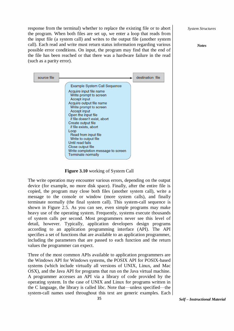
35

System Structures

Notes


response from the terminal) whether to replace the existing file or to abort

the program. When both files are set up, we enter a loop that reads from

the input file (a system call) and writes to the output file (another system

call). Each read and write must return status information regarding various

possible error conditions. On input, the program may find that the end of

the file has been reached or that there was a hardware failure in the read

(such as a parity error).

Figure 3.10 working of System Call

The write operation may encounter various errors, depending on the output

device (for example, no more disk space). Finally, after the entire file is

copied, the program may close both files (another system call), write a

message to the console or window (more system calls), and finally

terminate normally (the final system call). This system-call sequence is

shown in Figure 2.5. As you can see, even simple programs may make

heavy use of the operating system. Frequently, systems execute thousands

of system calls per second. Most programmers never see this level of

detail, however. Typically, application developers design programs

according to an application programming interface (API). The API

specifies a set of functions that are available to an application programmer,

including the parameters that are passed to each function and the return

values the programmer can expect.

Three of the most common APIs available to application programmers are

the Windows API for Windows systems, the POSIX API for POSIX-based

systems (which include virtually all versions of UNIX, Linux, and Mac

OSX), and the Java API for programs that run on the Java virtual machine.

A programmer accesses an API via a library of code provided by the

operating system. In the case of UNIX and Linux for programs written in

the C language, the library is called libc. Note that—unless specified—the

system-call names used throughout this text are generic examples. Each

36

System Structures

Notes


operating system has its own name for each system call. Behind the scenes,

the functions that make up an API typically invoke the actual system calls

on behalf of the application programmer.

There are several reasons for doing so. One benefit concerns program

portability. An application programmer designing a program using an API

can expect her program to compile and run on any system that supports the

same API (although, in reality, architectural differences often make this

more difficult than it may appear). Furthermore, actual system calls can

often be more detailed and difficult to work with than the API available to

an application programmer. Nevertheless, there often exists a strong

correlation between a function in the API and its associated system call

within the kernel. In fact, many of the POSIX and Windows APIs are

similar to the native system calls provided by the UNIX, Linux, and

Windows operating systems. For most programming languages, the run-

time support system (a set of functions built into libraries included with a

compiler) provides a system call interface that serves as the link to system

calls made available by the operating system. The system-call interface

intercepts function calls in the API and invokes the necessary system calls

within the operating system. Typically, a number is associated with each

system call, and the system-call interface maintains a table indexed

according to these numbers. The system call interface then invokes the

intended system call in the operating-system kernel and returns the status

of the system call and any return values.

The caller need know nothing about how the system call is implemented or

what it does during execution. Rather, the caller need only obey the API

and understand what the operating system will do as a result of the

execution of that system call. Thus, most of the details of the operating-

system interface are hidden from the programmer by the API and are

managed by the run-time

37

System Structures

Notes


Figure 3.11 using application call ()

Support library. The relationship between an API, the system-call

interface, and the operating system is shown in Figure 2.6, which illustrates

how the operating system handles a user application invoking the open()

system call. System calls occur in different ways, depending on the

computer in use. Often, more information is required than simply the

identity of the desired

System call. The exact type and amount of information vary according to

the particular operating system and call.

Figure 3.12 Parameter passing

For example, to get input, we may need to specify the file or device to use

as the source, as well as the address and length of the memory buffer into

38

System Structures

Notes


which the input should be read. Of course, the device or file and length

may be implicit in the call. Three general methods are used to pass

parameters to the operating system. The simplest approach is to pass the

parameters in registers. In some cases, however, there may be more

parameters than registers. In these cases, the parameters are generally

stored in a block, or table, in memory, and the address of the block is

passed as a parameter in a register (Figure 2.7). This is the approach taken

by Linux and Solaris. Parameters also can be placed, or pushed, onto the

stack by the program and popped off the stack by the operating system.

Some operating systems prefer the block or stack method because those

approaches do not limit the number or length of parameters being passed.

3.5.1 Types of System Calls

System calls can be grouped roughly into five major categories: process

control, file manipulation, device manipulation, information maintenance,

and communications.

Process control

o end, abort

o load, execute

o create process, terminate process

o get process attributes, set process attributes

o wait for time

o wait event, signal event

o allocate and free memory

File management

o create file, delete file

o open, close

o read, write, reposition

o get file attributes, set file attributes

Device management

o request device, release device

o read, write, reposition

o get device attributes, set device attributes

o logically attach or detach devices

Information maintenance

o get time or date, set time or date

o get system data, set system data

o get process, file, or device attributes

o set process, file, or device attributes

Communications

o create, delete communication connection

o send, receive messages

o transfer status information

o attach or detach remote devices

39

System Structures

Notes


3.6 SYSTEM PROGRAMS

System programs provide a convenient environment for program

development and execution.

This can be divided into:

o File management - Create, delete, copy, rename, print,

dump, list, and generally manipulate files and directories

o Status information

Some ask the system for info - date, time, amount of

available memory, disk space, number of users

Others provide detailed performance, logging, and

debugging information

Typically, these programs format and print the

output to the terminal or other output devices

Some systems implement a registry - used to store

and retrieve configuration information

o File modification- Several text editors may be available to

create and modify the content of files stored on disk or other

storage devices. There may also be special commands to

search contents of files or perform transformations of the

text.

o Programming-language support - Compilers, assemblers,

debuggers and interpreters for common programming

languages (such as C, C++, Java, Visual Basic, and PERL)

are often provided to the user with the operating system.

o Program loading and execution - Once a program is

assembled or compiled, it must be loaded into memory to be

executed. The system may provide absolute loaders,

relocatable loaders, linkage editors, and overlay loaders.

Debugging systems for either higher-level languages or

machine language are needed as well.

o Communications - Provide the mechanism for creating

virtual connections among processes, users, and computer

systems. They allow users to send messages to one

another’s screens, browse web pages, send electronic-mail

messages, log in remotely, transfer files from one machine

to another

Most users’ view of the operation system is defined by system

programs, not the actual system calls

Some of them are simply user interfaces to system calls; others are

considerably more complex

In addition to systems programs, most operating systems are

supplied with programs that are useful in solving common

problems or performing common operations. Such programs

include web browsers, word processors and text formatters,

spreadsheets, database systems, compilers, plotting and statistical-

analysis packages, and games. These programs are known as

system utilities or application programs.

40

System Structures

Notes


3.7 OPERATING-SYSTEM DESIGN AND

IMPLEMENTATION

Early operating systems were written in assembly language. Now, although

some operating systems are still written in assembly language, most are

written in a higher-level language such as C or an even higher-level

language such as C++. Actually, an operating system can be written in

more than one language.

The lowest levels of the kernel might be assembly language. Higher-level

routines might be in C, and system programs might be in C or C++, in

interpreted scripting languages like PERL or Python, or in shell scripts. In

fact, a given Linux distribution probably includes programs written in all

of those languages.

The first system that was not written in assembly language was probably

the Master Control Program (MCP) for Burroughs computers. MCP was

written in a variant of ALGOL. MULTICS, developed at MIT, was written

mainly in the system programming language PL/1. The Linux and

Windows operating system kernels are written mostly in C, although there

are some small sections of assembly code for device drivers and for saving

and restoring the state of registers.

The advantages of using a higher-level language, or at least a systems

implementation Language, for implementing operating systems are the

same as those gained when the language is used for application programs:

the code can be written faster, is more compact, and is easier to understand

and debug.

In addition, improvements in compiler technology will improve the

generated code for the entire operating system by simple recompilation.

Finally, an operating system is far easier to port—to move to some other

hardware— if it is written in a higher-level language. For example, MS-

DOS was written in Intel 8088 assembly language. Consequently, it runs

natively only on the Intel X86 family of CPUs. (Note that although MS-

DOS runs natively only on Intel X86, emulators of the X86 instruction set

allow the operating system to run on other CPUs—but more slowly, and

with higher resource use. The only possible disadvantages of implementing

an operating system in a higher-level language are reduced speed and

increased storage requirements.

This, however, is no longer a major issue in today’s systems. Although an

expert assembly-language programmer can produce efficient small

routines, for large programs a modern compiler can perform complex

analysis and apply sophisticated optimizations that produce excellent code.

Modern processors have deep pipelining and multiple functional units that

can handle the details of complex dependencies much more easily than can

the human mind. As is true in other systems, major performance

41

System Structures

Notes


improvements in operating systems are more likely to be the result of

better data structures and algorithms than of excellent assembly-language

code. In addition, although operating systems are large, only a small

amount of the code is critical to high performance; the interrupt handler,

I/O manager, memory manager, and CPU scheduler are probably the most

critical routines.

Check your Progress

1. What are system calls?

2. What are the types of system calls?

3. What are the types of Loadable kernel modules?

4. What is the difference between microkernel and macro kernel?

5. What are System Programs?


1. System calls provide the interface between a process and the

operating system. System calls for modern Microsoft windows

platforms are part of the win32 API, which is available for all the

compilers written for Microsoft windows.

2. System calls can be grouped roughly into five major categories:

process control

file manipulation

device manipulation

information maintenance

communications.

3. A core kernel with seven types of loadable kernel modules:

Scheduling classes

File systems

Loadable system calls

Executable formats

STREAMS modules

Miscellaneous

Device and bus drivers

4. Some of the difference are:

Micro-Kernel : A micro-kernel is a minimal operating

system that performs only the essential functions of an

operating system. All other operating system functions are

performed by system processes.

Monolithic : A monolithic operating system is one where

all operating system code is in a single executable image

and all operating system code runs in system mode.

5. System programs provide a convenient environment for program

development and execution. This can be divided into:

File management

Status information

42

System Structures

Notes


File modification

Programming-language support

Program loading and execution

Communications

3.9. SUMMARY The main function of the microkernel is to provide

communication between the client program and the various

services that are also running in user space.

The idea of the design is for the kernel to provide core services

while other services are implemented dynamically, as the kernel

is running.

The Solaris operating system structure is organized around a

core kernel with seven types of loadable kernel modules

iOS is a mobile operating system designed by Apple to run its

smartphone, the iPhone, as well as its tablet computer, the iPad.

The Android operating system was designed by the Open

Handset Alliance (led primarily by Google) and was developed

for Android smartphones and tablet computers.

System calls can be grouped roughly into five major categories:

process control, file manipulation, device manipulation,

information maintenance, and communications.

3.10. KEYWORDS

Program execution: The system must be able to load a program

into memory and to run that program. The program must be able to

end its execution, either normally or abnormally (indicating error).

I/O operations: A running program may require I/O, which may

involve a file or an I/O device.

Resource allocation: When there are multiple users or multiple

jobs running at the same time, resources must be allocated to each

of them.

System calls: System calls provide an interface to the services

made available by an operating system.

3.11. SELF ASSESSMENT QUESTIONS AND

EXERCISES


1. What are Modules?

2. What is layered approach?

3. What are Hybrid systems?

4. What is Resource allocation?

5. Explain about Layered operating system?

43

System Structures

Notes



1. Explain about system calls and its types?

2. Explain about Operating-System Design and his Implementation?

3. Explain about system programs and its types?

3.12 FURTHER READINGS









44

Process Concept

Notes


BLOCK – II INTRODUCTION

UNIT IV PROCESS CONCEPT

Structure 4.0 Introduction

4.1 Objective

4.2 Process Concept


4.4Operations on Processes



4.5 Inter process Communication


4.7 Summary

4.8 Key Words



4.0 INTRODUCTION

he scheduling of process is a tedious task and needs to organized to

perform this effectively the operating system introduces a concept process

scheduling and the various operations on process in explaining by how it is

performed. The process scheduling is the activity of the process manager

that handles the removal of the running process from the CPU and the

selection of another process on the basis of a particular strategy.

Process scheduling is an essential part of a Multiprogramming operating

systems. Such operating systems allow more than one process to be loaded

into the executable memory at a time and the loaded process shares the

CPU using time multiplexing. The inter process communication between

the system is also explained.

4.1 OBJECTIVE

This unit helps to understand the

Process scheduling concepts

Various operations on process

Inter process communication

45

Process Concept

Notes


4.2 PROCESS CONCEPT

A batch system executes jobs, whereas a time-shared system has user

programs, or tasks. Even on a single-user system, a user maybe able to run

several programs at one time: a word processor, a Web browser, and an e-

mail package. And even if a user can execute only one program at a time,

such as on an embedded device that does not support multitasking, the

operating system may need to support its own internal programmed

activities, such as memory management. In many respects, all these

activities are similar, so we call all of them processes. The terms job and

process are used almost interchangeably in this text. Although we

personally prefer the term process, much of operating-system theory and

terminology was developed during a time when the major activity of

operating systems was job processing. It would be misleading to avoid the

use of commonly accepted terms that include the word job simply because

process has superseded job.

4.2.1The Process

A program becomes a process when an executable file is loaded into

memory. Two common techniques for loading executable files are double-

clicking an icon representing the executable file and entering the name of

the executable file on the command line (as in prog.exe or a. out).

Although two processes may be associated with the same program, they

are nevertheless considered two separate execution sequences. For

instance, several users may be running different copies of the mail

program, or the same user may invoke many copies of the web browser

program. Each of these is a separate process; and although the text sections

are equivalent, the data, heap, and stack sections vary. It is also common to

have a process that spawns many processes as it runs. Note that a process

itself can be an execution environment for other code. The Java

programming environment provides a good example. In most

circumstances, an executable Java program is executed within the Java

virtual machine (JVM). The JVM executes as a process that interprets the

loaded Java code and takes actions (via native machine instructions) on

behalf of that code.

For example, to run the compiled Java program. Class, we would enter

java Program the command java runs the JVM as an ordinary process,

which in turns executes the Java program in the virtual machine. The

concept is the same as simulation, except that the code, instead of being

written for a different instruction set, is written in the Java language

46

Process Concept

Notes


Figure 4.1 Processes in a Memory

4.2.2 Process State

As a process executes, it changes state. The state of a process is defined in

part by the current activity of that process. A process may be in one of the

following states:

• New. The process is being created.

• Running. Instructions are being executed.

• Waiting. The process is waiting for some event to occur (such as an I/O

completion or reception of a signal).

• Ready. The process is waiting to be assigned to a processor.

• Terminated. The process has finished execution.

These names are arbitrary, and they vary across operating systems. The

states that they represent are found on all systems, however. Certain

operating systems also more finely delineate process states. It is important

to realize that only one process can be running on any processor at any

instant. Many processes may be ready and waiting, however. The state

diagram corresponding to these states is presented in Figure

4.2.3 Process Control Block

Each process is represented in the operating system by a process control

block (PCB)—also called a task control block. APCB is shown in Figure

47

Process Concept

Notes


3.3. It contains many pieces of information associated with a specific

process, including these:

Process state. The state may be new, ready, running, waiting,

halted, and so on.

Program counter. The counter indicates the address of the next

instruction to be executed for this process.

CPU registers. The registers vary in number and type, depending

on the computer architecture. They include accumulators, index

registers, stack pointers, and general-purpose registers, plus any

condition-code information. Along with the program counter, this

state information must be saved when an interrupt occurs, to allow

the process to be continued correctly afterward

CPU-scheduling information. This information includes a process

priority, pointers to scheduling queues, and any other scheduling

parameters.

Memory-management information. This information may

include such items as the value of the base and limit registers and

the page tables, or the segment tables, depending on the memory

system used by the operating system.

Figure 4.2 Process State

Accounting information. This information includes the amount of

CPU and real time used, time limits, account numbers, job or

process numbers, and so on.

I/O status information. This information includes the list of I/O

devices allocated to the process, a list of open files, and so on.

48

Process Concept

Notes


Figure 4.3 Process control Block

Figure 4.4 CPU switch from process to process

49

Process Concept

Notes


4.2.4 Threads

The process model discussed so far has implied that a process is a program

that performs a single thread of execution. For example, when a process is

running a word-processor program, a single thread of instructions is being

executed. This single thread of control allows the process to perform only

one task at a time. The user cannot simultaneously type in characters and

run the spell checker within the same process, for example. Most modern

operating systems have extended the process concept to allow a process to

have multiple threads of execution and thus to perform more than one task

at a time. This feature is especially beneficial on multicore systems, where

multiple threads can run in parallel. On a system that supports threads, the

PCB is expanded to include information for each thread. Other changes

throughout the system are also needed to support threads.

4.3 PROCESS SCHEDULING

The objective of multiprogramming is to have some process running at all

times, to maximize CPU utilization. The objective of time sharing is to

switch then CPU among processes so frequently that users can interact

with each program while it is running. To meet these objectives, the

process scheduler selects an available process for program execution on the

CPU. For a single-processor system, there will never be more than one

running process. If there are more processes, the rest will have to wait until

the CPU is free and can be rescheduled.

4.4 OPERATIONS ON PROCESSES

The processes in most systems can execute concurrently, and they may be

created and deleted dynamically. Thus, these systems must provide a

mechanism for process creation and termination. In this section, we

explore the mechanisms involved in creating processes and illustrate

process creation on UNIX and Windows systems


During the course of execution, a process may create several new

processes. As mentioned earlier, the creating process is called a parent

process, and the new processes are called the children of that process. Each

of these new processes may in turn create other processes, forming a tree

of processes. Most operating systems (including UNIX, Linux, and

Windows) identify processes according to a unique process identifier (or

pid), which is typically an integer number. The pid provides a unique value

for each process in the system, and it can be used as an index to access

various attributes of a process within the kernel. Figure 3.8 illustrates a

typical process tree for the Linux operating system, showing the name of

each process and it’s pid. (We use the term process rather loosely, as Linux

prefers the term task instead.) The init process (which always has a pid of

1) serves as the root parent process for all user processes. Once the system

has booted, the init process can also create various user processes, such as

a web or print server, an ssh server, and the like.

50

Process Concept

Notes


The kthreadd process is responsible for creating additional processes that

perform tasks on behalf of the kernel (in this situation, khelper and

pdflush). The sshd process is responsible for managing clients that connect

to the system by using ssh (which is short for secure shell). The login

process is responsible for managing clients that directly log onto the

system. In this example, a client has logged on and is using the bash shell,

which has been assigned pid 8416. Using the bash command-line interface,

this user has created the process ps as well as the emacs editor. On UNIX

and Linux systems, we can obtain a listing of processes by using the ps

command. For example, the command ps –el will list complete information

for all processes currently active in the system.

In general, when a process creates a child process, that child process will

need certain resources (CPU time, memory, files, I/O devices) to

accomplish its task. A child process may be able to obtain its resources

directly from the operating system, or it may be constrained to a subset of

the resources of the parent process. The parent may have to partition its

resources among its children, or it may be able to share some resources

(such as memory or files) among several of its children. Restricting a child

process to a subset of the parent’s resources prevents any process from

overloading the system by creating too many child processes. In addition to

supplying various physical and logical resources, the parent process may

pass along initialization data (input) to the child process. For example,

consider a process whose function is to display the contents of a file —say,

image.jpg—on the screen of a terminal. When the process is created, it will

get, as an input from its parent process, the name of the file image.jpg.

Using that file name, it will open the file and write the contents out. It may

also get the name of the output device. Alternatively, some operating

systems pass resources to child processes. On such a system, the new

process may get two open files, image.jpg and the terminal device, and

may simply transfer the datum between the two. When a process creates a

new process, two possibilities for execution exist:

1. The parent continues to execute concurrently with its children.

2. The parent waits until some or all of its children have terminated.

There are also two address-space possibilities for the new process:

1. The child process is a duplicate of the parent process (it has the same

program and data as the parent).

2. The child process has a new program loaded into it.

In UNIX, as we’ve seen, each process is identified by its process

identifier, which is a unique integer. A new process is created by the fork()

system call. The new process consists of a copy of the address space of the

original process. This mechanism allows the parent process to

communicate easily with its child process. Both processes (the parent and

the child) continue execution at the instruction after the fork(), with one

difference: the return code for the fork() is zero for the new (child) process,

51

Process Concept

Notes


whereas the (nonzero) process identifier of the child is returned to the

parent. After a fork() system call, one of the two processes typically uses

the exec() system call to replace the process’s memory space with a new

program.

The exec() system call loads a binary file into memory (destroying the

memory image of the program containing the exec() system call) and starts

its execution. In this manner, the two processes are able to communicate

and then go their separate ways. The parent can then create more children;

or, if it has nothing else to do while the child runs, it can issue a wait()

system call to move itself off the ready queue until the termination of the

child. Because the call to exec() overlays the process’s address space with a new

program, the call to exec() does not return control unless an error occurs.

The only difference is that the value of pi value greater than zero (in fact,

it is the actual pid of the child process). The child process inherits

privileges and scheduling attributes from the parent, as well certain

resources, such as open files. The child process then overlays its address

space with the UNIX command /bin/ls (used to get a directory listing)

using the execlp() system call (execlp() is a version of the exec() system

call). The parent waits for the child process to complete with the wait()

system call. When the child process completes (by either implicitly or

explicitly invoking exit()), the parent process resumes from the call to

wait(), where it completes using the exit() system call.

Of course, there is nothing to prevent the child from not invoking exec()

and instead continuing to execute as a copy of the parent process. In this

scenario, the parent and child are concurrent processes running the same

code instructions. Because the child is a copy of the parent, each process

has its own copy of any data. As an alternative example, we next consider

process creation in Windows. Processes are created in the Windows API

using the CreateProcess() function, which is similar to fork() in that a

parent creates a new child process. However, whereas fork() has the child

process inheriting the address space of its parent, CreateProcess() requires

loading a specified program into the address space of the child process at

process creation. Furthermore, whereas fork() is passed no parameters,

CreateProcess() expects no fewer than ten parameters.

We opt for many of the default values of the ten parameters passed to

CreateProcess(). Readers interested in pursuing the details of process

creation and management in the Windows API are encouraged to consult

the bibliographical notes at the end of this chapter. The two parameters

passed to the CreateProcess() function are instances of the

STARTUPINFO and PROCESS INFORMATION structures.

STARTUPINFO specifies many properties of the new process, such as

window size and appearance and handles to standard input and output files.

The PROCESS INFORMATION structure contains a handle and the

identifiers to the newly created process and its thread. We invoke the

ZeroMemory() function to allocate memory for each of these structures

before proceeding with CreateProcess().

52

Process Concept

Notes


The first two parameters passed to CreateProcess() are the application

name and command-line parameters. If the application name is NULL (as

it is in this case), the command-line parameter specifies the application to

load. In this instance, we are loading the Microsoft Windows mspaint.exe

application. Beyond these two initial parameters, we use the default

parameters for inheriting process and thread handles as well as specifying

that there will be no creation flags. Also use the parent’s existing

environment block and starting directory. Last, we provide two pointers to

the STARTUPINFO and PROCESS - INFORMATION structures created

at the beginning of the program.


A process terminates when it finishes executing its final statement and asks

the operating system to delete it by using the exit() system call. At that

point, then process may return a status value (typically an integer) to its

parent process (via the wait() system call). All the resources of the

process—including physical and virtual memory, open files, and I/O

buffers—are deallocated by the operating system. Termination can occur in

other circumstances as well. A process can cause the termination of

another process via an appropriate system call (for example,

TerminateProcess() in Windows).

Usually, such a system call can be invoked only by the parent of the process

that is to be terminated. Otherwise, users could arbitrarily kill each other’s jobs.

Note that a parent needs to know the identities of its children if it is to

terminate them. Thus, when one process creates a new process, the identity

of the newly created process is passed to the parent. A parent may

terminate the execution of one of its children for a variety of reasons, such

as these:

The child has exceeded its usage of some of the

resources that it has been allocated. (To determine

whether this has occurred, the parent must have a

mechanism to inspect the state of its children.)

The task assigned to the child is no longer required.

The parent is exiting, and the operating system does

not allow a child to continue if its parent terminates.

Some systems do not allow a child to exist if its parent has terminated. In

such systems, if a process terminates (either normally or abnormally), then

all its children must also be terminated.

This phenomenon, referred to as cascading termination, is normally

initiated by the operating system. To illustrate process execution and

termination, consider that, in Linux and UNIX systems, we can terminate a

process by using the exit() system call, providing an exit status as a

parameter:

/* exit with status 1 */

53

Process Concept

Notes


exit(1);

In fact, under normal termination, exit() may be called either directly (as

shown above) or indirectly (by a return statement in main()). A parent

process may wait for the termination of a child process by using the wait()

system call. The wait() system call is passed a parameter that allows the

parent to obtain the exit status of the child. This system call also returns the

process identifier of the terminated child so that the parent can tell which

of its children has terminated:

pid t pid;

int status;

pid = wait(&status);

When a process terminates, its resources are deallocated by the operating

system. However, its entry in the process table must remain there until the

parent calls wait(), because the process table contains the process’s exit

status. A process that has terminated, but whose parent has not yet called

wait(), is known as a zombie process. All processes transition to this state

when they terminate, but generally they exist as zombies only briefly.

Once the parent calls wait(), the process identifier of the zombie process

and its entry in the process table are released. Now consider what would

happen if a parent did not invoke wait() and instead terminated, thereby

leaving its child processes as orphans. Linux and UNIX address this

scenario by assigning the init process as the new parent to orphan

processes. The init process periodically invokes wait(), thereby allowing

the exit status of any orphaned process to be collected and releasing the

orphan’s process identifier and process-table entry.

4.5 INTERPROCESS COMMUNICATION

Processes executing concurrently in the operating system may be either

independent processes or cooperating processes. A process is independent

if it cannot affect or be affected by the other processes executing in the

system. Any process that does not share data with any other process is

independent. A process is cooperating if it can affect or be affected by the

other processes executing in the system. Clearly, any process that shares

data with other processes is a cooperating process. There are several

reasons for providing an environment that allows process cooperation:

• Information sharing. Since several users may be interested in the same

piece of information (for instance, a shared file), we must provide an

environment to allow concurrent access to such information.

• Computation speedup. If we want a particular task to run faster, we

must break it into subtasks, each of which will be executing in parallel with

54

Process Concept

Notes


the others. Notice that such a speedup can be achieved only if the computer

has multiple processing cores.

• Modularity. We may want to construct the system in a modular fashion,

dividing the system functions into separate processes or threads, as we

discussed in Chapter 2.

• Convenience. Even an individual user may work on many tasks at the

same time. For instance, a user may be editing, listening to music, and

compiling in parallel.

Cooperating processes require an interprocess communication (IPC)

mechanism that will allow them to exchange data and information. There

are two fundamental models of interprocess communication: shared

memory and message passing. In the shared-memory model, a region of

memory that is shared by cooperating processes is established. Processes

can then exchange information by reading and writing data to the shared

region. In the message-passing model, communication takes place by

means of messages exchanged between the cooperating processes.

Both of the models just mentioned are common in operating systems, and

many systems implement both. Message passing is useful for exchanging

smaller amounts of data, because no conflicts need be avoided. Message

passing is also easier to implement in a distributed system than shared

memory. (Although there are systems that provide distributed shared

memory, we do not consider them in this text

Shared memory can be faster than message passing, since message-passing

systems are typically implemented using system calls and thus require the

more time-consuming task of kernel intervention. In shared-memory

systems, system calls are required only to establish shared memory

regions. Once shared memory is established, all accesses are treated as

routine memory accesses, and no assistance from the kernel is required.

Recent research on systems with several processing cores indicates that

message passing provides better performance than shared memory on such

systems. Shared memory suffers from cache coherency issues, which arise

because shared data migrate among the several caches. As the number of

processing cores on systems increases, it is possible that we will see

message passing as the preferred mechanism for IPC. In the remainder of

this section, we explore shared-memory and message passing systems in

more detail.

4.5.1 Shared-Memory Systems

Interprocess communication using shared memory requires communicating

processes to establish a region of shared memory. Typically, a shared-

memory region resides in the address space of the process creating the

shared-memory segment. Other processes that wish to communicate using

this shared-memory segment must attach it to their address space. Recall

that, normally, the operating system tries to prevent one process from

accessing another process’s memory. Shared memory requires that two or

55

Process Concept

Notes


more processes agree to remove this restriction. They can then exchange

information by reading and writing data in the shared areas. The form of

the data and the location are determined by these processes and are not

under the operating system’s control. The processes are also responsible

for ensuring that they are not writing to the same location simultaneously.

To illustrate the concept of cooperating processes, let’s consider the

producer–consumer problem, which is a common paradigm for

cooperating processes.

A producer process produces information that is consumed by a consumer

process. For example, a compiler may produce assembly code that is

consumed by an assembler. The assembler, in turn, may produce object

modules that are consumed by the loader. The producer–consumer problem

also provides a useful metaphor for the client–server paradigm. Generally

think of a server as a producer and a client as a consumer. For example, a

webserver produces (that is, provides) HTML files and images, which are

consumed (that is, read) by the client web browser requesting the resource.

One solution to the producer–consumer problem uses shared memory. To

allow producer and consumer processes to run concurrently, we must have

available a buffer of items that can be filled by the producer and emptied

by the consumer. This buffer will reside in a region of memory that is

shared by the producer and consumer processes. A producer can produce

one item while the consumer is consuming another item. The producer and

consumer must be synchronized, so that the consumer does not try to

consume an item that has not yet been produced. Two types of buffers can

be used. The unbounded buffer places no practical limit on the size of the

buffer.

The consumer may have to wait for new items, but the producer can

always produce new items. The bounded buffer assumes a fixed buffer

size. In this case, the consumer must wait if the buffer is empty, and the

producer must wait if the buffer is full.Let’s look more closely at how the

bounded buffer illustrates interprocess communication using shared

memory. The following variables reside in a region of memory shared by

the producer and consumer processes:

#define BUFFER SIZE 10

typedef struct {

. . .

}item;

item buffer[BUFFER SIZE];

int in = 0;

int out = 0;

The shared buffer is implemented as a circular array with two logical

pointers: in and out. The variable in points to the next free position in the

56

Process Concept

Notes


buffer; out points to the first full position in the buffer. The buffer is empty

when in == out; the buffer is full when ((in + 1) % BUFFER SIZE) == out.

The producer process has a local variable next produced in which the new

item to be produced is stored. The consumer process has a local variable

next consumed in which the item to be consumed is stored.

This scheme allows at most BUFFER SIZE − 1 items in the buffer at the

same time. We leave it as an exercise for you to provide a solution in

which BUFFER SIZE items can be in the buffer at the same time. In

Section 3.5.1, illustrates the POSIX API for shared memory. One issue this

illustration does not address concerns the situation in which both the

producer process and the consumer process attempt to access the shared

buffer concurrently. In Chapter 5, we discuss how synchronization among

cooperating processes can be implemented effectively in a shared memory

environment.

4.5.2 Message-Passing Systems

The scheme requires that these processes share a region of memory and

that the code for accessing and manipulating the shared memory be written

explicitly by the application programmer. Another way to achieve the same

effect is for the operating system to provide the means for cooperating

processes to communicate with each other via a message-passing facility.

Message passing provides a mechanism to allow processes to communicate

and to synchronize their actions without sharing the same address space. It

is particularly useful in a distributed environment, where the

communicating processes may reside on different computers connected by

a network. For example, an Internet chat program could be designed so that

chat participants communicate with one another by exchanging messages.

A message-passing facility provides at least two operations: send(message)

receive(message) Messages sent by a process can be either fixed or

variable in size. If only fixed-sized messages can be sent, the system-level

implementation is straightforward.

This restriction, however, makes the task of programming more difficult.

Conversely, variable-sized messages require a more complex system level

implementation, but the programming task becomes simpler. This is a

common kind of tradeoff seen throughout operating-system design. If

processes P and want to communicate, they must send messages to and

receive messages from each other: a communication link must exist

between them. This link can be implemented in a variety of ways. We are

concerned here not with the link’s physical implementation (such as shared

memory, hardware bus, or network, which are covered in Chapter 17) but

rather with its logical implementation. Here are several methods for

logically implementing a link and the send()/receive() operations:

• Direct or indirect communication

• Synchronous or asynchronous communication

• Automatic or explicit buffering

57

Process Concept

Notes


4.5.2.1 Naming

Processes that want to communicate must have a way to refer to each

other. They can use either direct or indirect communication. Under direct

communication, each process that wants to communicate must explicitly

name the recipient or sender of the communication. In this scheme, the

send() and receive() primitives are defined as:

• send(P, message)—Send a message to process P.

• receive(Q, message)—Receive a message from process Q.

A communication link in this scheme has the following properties:

• A link is established automatically between every pair of processes that

want to communicate. The processes need to know only each other’s

identity to communicate.

• A link is associated with exactly two processes.

• Between each pair of processes, there exists exactly one link.

This scheme exhibits symmetry in addressing; that is, both the sender

process and the receiver process must name the other to communicate. A

variant of this scheme employs asymmetry in addressing. Here, only the

sender names the recipient; the recipient is not required to name the sender.

In this scheme, the send() and receive() primitives are defined as follows:

• send(P, message)—Send a message to

• receive(id, message)—Receive a message from any process. The process

P. variable id is set to the name of the process with which communication

has taken place. The disadvantage in both of these schemes (symmetric and

asymmetric) is the limited modularity of the resulting process definitions.

Changing the identifier of a process may necessitate examining all other

process definitions. All references to the old identifier must be found, so

that they can be modified to the new identifier. In general, any such hard-

coding techniques, where identifiers must be explicitly stated, are less

desirable than techniques involving indirection, as described next. With

indirect communication, the messages are sent to and received from

mailboxes, or ports. Mailbox can be viewed abstractly as an object into

which messages can be placed by processes and from which messages can

be removed.

Each mailbox has a unique identification. For example, POSIX message

queues use an integer value to identify a mailbox. A process can

communicate with another process via a number of different mailboxes,

but two processes can communicate only if they have a shared mailbox.

The send() and receive() primitives are defined as follows:

• send(A, message)—Send a message to mailbox A.

• receive(A, message)—Receive a message from mailbox A.

58

Process Concept

Notes


In this scheme, a communication link has the following properties:

• A link is established between a pair of processes only if both members of

the pair have a shared mailbox.

• A link may be associated with more than two processes.

• Between each pair of communicating processes, a number of different

links may exist, with each link corresponding to one mailbox. Now

suppose that processes P1, P2, and P3 all share mailbox A. Process P1

sends a message to A, while both P2 and P3 execute a receive() from A.

Which process will receive the message sent by P1? The answer depends

on which of the following methods we choose:

• Allow a link to be associated with two processes at most.

• Allow at most one process at a time to execute a receive() operation.

• Allow the system to select arbitrarily which process will receive the

message (that is, either P2 or P3, but not both, will receive the message).

The system may define an algorithm for selecting which process will

receive the message (for example, round robin, where processes take turns

receiving messages). The system may identify the receiver to the sender. A

mailbox may be owned either by a process or by the operating system.

If the mailbox is owned by a process (that is, the mailbox is part of the

address space of the process), then we distinguish between the owner

(which can only receive messages through this mailbox) and the user

(which can only send messages to the mailbox). Since each mailbox has a

unique owner, there can be no confusion about which process should

receive a message sent to this mailbox. When a process that owns a

mailbox terminates, the mailbox disappears. Any process that subsequently

sends a message to this mailbox must be notified that the mailbox no

longer exists. In contrast, a mailbox that is owned by the operating system

has an existence of its own. It is independent and is not attached to any

particular process. The operating system then must provide a mechanism

that allows a process to do the following:

• Create a new mailbox.

• Send and receive messages through the mailbox.

• Delete a mailbox.

The process that creates a new mailbox is that mailbox’s owner by default.

Initially, the owner is the only process that can receive messages through

this mailbox. However, the ownership and receiving privilege may be

passed to other processes through appropriate system calls. Of course, this

provision could result in multiple receivers for each mailbox.

59

Process Concept

Notes


4.5.2.2 Synchronization

Communication between processes takes place through calls to send() and

receive() primitives. There are different design options for implementing

each primitive. Message passing may be either blocking or nonblocking—

also known as synchronous and asynchronous. (Throughout this text, you

will encounter the concepts of synchronous and asynchronous behavior in

relation to various operating-system algorithms.)

• Blocking send. The sending process is blocked until the message is

received by the receiving process or by the mailbox.

• Nonblocking send. The sending process sends the message and resumes

operation.

• Blocking receive. The receiver blocks until a message is available.

• Nonblocking receive. The receiver retrieves either a valid message or a

null.

Different combinations of send() and receive() are possible.When both

send() and receive() are blocking, we have a rendezvous between the

sender and the receiver. The solution to the producer–consumer problem

becomes trivial when we use blocking send() and receive() statements. The

producer merely invokes the blocking send() call and waits until the

message is delivered to either the receiver or the mailbox. Likewise, when

the consumer invokes receive(), it blocks until a message is available.

4.5.2.3 Buffering

Whether communication is direct or indirect, messages exchanged by

communicating processes reside in a temporary queue. Basically, such

queues can be implemented in three ways:

Zero capacity. The queue has a maximum length of zero; thus, the

link cannot have any messages waiting in it. In this case, the sender

must block until the recipient receives the message.

• Bounded capacity. The queue has finite length n; thus, at most n

messages can reside in it. If the queue is not full when a new message is

sent, the message is placed in the queue (either the message is copied or a

pointer to the message is kept), and the sender can continue execution

without waiting. The link’s capacity is finite, however. If the link is full,

the sender must block until space is available in the queue.

• Unbounded capacity. The queue’s length is potentially infinite; thus,

any number of messages can wait in it. The sender never blocks. The zero-

capacity case is sometimes referred to as a message system with no

buffering. The other cases are referred to as systems with automatic

buffering

60

Process Concept

Notes


Check your Progress

1. What is a process?

2. What are the states of a process?

3. What are the process control block?

4. What is Thread?

5. What is Process Termination?

4.6 ANSWERS TO CHECK YOUR PROGRESS

1. A program in execution is called a process. Or it may also be called

a unit of work. A process needs some system resources as CPU

time, memory, files, and i/o devices to accomplish the task. Each

process is represented in the operating system by a process control

block or task control block (PCB). Processes are of two types

Operating system processes

User processes

2. The states of process are:

New

Running

Waiting

Ready

Terminated

3. Process Control Block (PCB) contains many pieces of information

associated with a specific process, including these:

Process state.

Program counter.

CPU registers

CPU-scheduling information.

Memory-management information.

Accounting information

I/O status information.

4. A thread is a flow of execution through the process code, with its

own program counter that keeps track of which instruction to

execute next, system registers which hold its current working

variables.

5. A process terminates when it finishes executing its final statement

and asks the operating system to delete it by using the exit ()

system call. At that point, then process may return a status value

(typically an integer) to its parent process (via the wait () system

call). All the resources of the process—including physical and

virtual memory, open files, and I/O buffers—are deallocated by the

operating system. Termination can occur in other circumstances as

well. A process can cause the termination of another process via an

61

Process Concept

Notes


appropriate system call (for example, Terminate Process () in

Windows).

4.7. SUMMARY The objective of multiprogramming is to have some process

running at all times, to maximize CPU utilization.

A program becomes a process when an executable file is loaded

into memory.

A process terminates when it finishes executing its final

statement and asks the operating system to delete it by using the

exit() system call.

Interprocess communication using shared memory requires

communicating processes to establish a region of shared

memory.

Communication between processes takes place through calls to

send() and receive() primitives.

The queue’s length is potentially infinite; thus, any number of

messages can wait in it.

4.8. KEYWORDS CPU registers. The registers vary in number and type, depending on the

computer architecture. They include accumulators, index registers, stack

pointers, and general-purpose registers, plus any condition-code

information. Along with the program counter, this state information must

be saved when an interrupt occurs, to allow the process to be continued

correctly afterward

Information sharing. Since several users may be interested in the same

piece of information (for instance, a shared file), we must provide an

environment to allow concurrent access to such information.

CPU-scheduling information. This information includes a process

priority, pointers to scheduling queues, and any other scheduling

parameters.

Memory-management information. This information may include such

items as the value of the base and limit registers and the page tables, or the

segment tables, depending on the memory system used by the operating

system.


EXERCISES


1. What is interprocess communication?

2. What is process creation?

3. Explain about shared-memory systems?

4. What is Synchronization?

62

Process Concept

Notes


5. Explain the capacity of Buffering?


1. Explain about Operations on processes?

2. Explain about Interprocess Communication ?










63

Process Scheduling

Notes


UNIT V PROCESS SCHEDULING

Structure

5.0 Introduction

5.1 Objective


5.3 Scheduling Criteria

5.4 Scheduling Algorithms

5.5 Multiple-Processor Scheduling


5.7 Summary

5.8 Key Words



5.0 INTRODUCTION

The scheduling of the process in the operating system has to perform with

some criteria and there are many scheduling algorithms which work under

different constraints so as to schedule the process effectively. The OS

maintains all PCBs in Process Scheduling Queues. The OS maintains a

separate queue for each of the process states and PCBs of all processes in

the same execution state are placed in the same queue. When the state of a

process is changed, its PCB is unlinked from its current queue and moved

to its new state queue. This unit covers the scheduling algorithms with an

illustration of its working. The multiple processor scheduling is covered

with its working.

5.1 OBJECTIVE

This unit covers the following

Learn the scheduling algorithms

Understand the scheduling concepts

Explore the multiple processor scheduling

5.2 PROCESS SCHEDULING

5.2.1 Scheduling concepts

As processes enter the system, they are put into a job queue, which consists

of all processes in the system. The processes that are residing in main

memory and are ready and waiting to execute are kept on a list called the

ready queue. This queue is generally stored as a linked list. A ready-queue

header contains pointers to the first and final PCBs in the list. Each PCB

64

Process Scheduling

Notes


includes a pointer field that points to the next PCB in the ready queue. The

system also includes other queues. When a process is allocated the CPU, it

executes for a while and eventually quits, is interrupted, or waits for the

occurrence of a particular event, such as the completion of an I/O request.

Suppose the process makes an I/O request to a shared device, such as a

disk. Since there are many processes in the system, the disk may be busy

with the I/O request of some other process. The process therefore may

have to wait for the disk. The list of processes waiting for a particular I/O

device is called a device queue.

Figure 5.1 Ready Queue and I/O devices queue

A common representation of process scheduling is a queueing diagram,

such as that in Figure 5.1. Each rectangular box represents a queue. Two

types of queues are present: the ready queue and a set of device queues.

The circles represent the resources that serve the queues, and the arrows

indicate the flow of processes in the system. A new process is initially put

in the ready queue. It waits there until it is selected for execution, or

dispatched. Once the process is allocated the CPU and is executing, one of

several events could occur:

• The process could issue an I/O request and then be placed in an I/O

queue.

• The process could create a new child process and wait for the child’s

termination.

• The process could be removed forcibly from the CPU, as a result of an

interrupt, and be put back in the ready queue. In the first two cases, the

65

Process Scheduling

Notes


process eventually switches from the waiting state to the ready state and is

then put back in the ready queue. A process continues

This cycle until it terminates, at which time it is removed from all queues

and has its PCB and resources deallocated.

Figure 5.2 Process Scheduling Queuing

5.3 SCHEDULING CRITERIA

Different CPU-scheduling algorithms have different properties, and the

choice of a particular algorithm may favor one class of processes over

another. In choosing which algorithm to use in a particular situation, we

must consider the properties of the various algorithms. Many criteria have

been suggested for comparing CPU-scheduling algorithms. Which

characteristics are used for comparison can make a substantial difference in

which algorithm is judged to be best. The criteria include the following:

• CPU utilization. We want to keep the CPU as busy as possible.

Conceptually, CPU utilization can range from 0 to 100 percent. In a real

system, it should range from 40 percent (for a lightly loaded system) to 90

percent (for a heavily loaded system).

• Throughput. If the CPU is busy executing processes, then work is being

done. One measure of work is the number of processes that are completed

per time unit, called throughput. For long processes, this rate may be one

process per hour; for short transactions, it may be ten processes per second.

• Turnaround time. From the point of view of a particular process, the

important criterion is how long it takes to execute that process. The

interval from the time of submission of a process to the time of completion

is the turnaround time. Turnaround time is the sum of the periods spent

waiting to get into memory, waiting in the ready queue, executing on the

CPU, and doing I/O.

66

Process Scheduling

Notes


• Waiting time. The CPU-scheduling algorithm does not affect the amount

of time during which a process executes or does I/O. It affects only the

amount of time that a process spends waiting in the ready queue. Waiting

time is the sum of the periods spent waiting in the ready queue.

• Response time. In an interactive system, turnaround time may not be the

best criterion. Often, a process can produce some output fairly early and

can continue computing new results while previous results are being output

to the user. Thus, another measure is the time from the submission of a

request until the first response is produced. This measure, called response

time, is the time it takes to start responding, not the time it takes to output

the response.

The turnaround time is generally limited by the speed of the output device.

It is desirable to maximize CPU utilization and throughput and to minimize

turnaround time, waiting time, and response time. In most cases, we

optimize the average measure. However, under some circumstances, we

prefer to optimize the minimum or maximum values rather than the

average. For example, to guarantee that all users get good service, we may

want to minimize the maximum response time. Investigators have

suggested that, for interactive systems (such as desktop systems), it is more

important to minimize the variance in the response time than to minimize

the average response time. A system with reasonable and predictable

response time may be considered more desirable than a system that is

faster on the average but is highly variable.

However, little work has been done on CPU-scheduling algorithms that

minimize variance. As we discuss various CPU-scheduling algorithms in

the following section, we illustrate their operation. An accurate illustration

should involve many processes, each a sequence of several hundred CPU

bursts and I/O bursts. For simplicity, though, we consider only one CPU

burst (in milliseconds) per process in our examples.

5.4 SCHEDULING ALGORITHMS

5.4.1 First-Come, First-Served Scheduling

By far the simplest CPU-scheduling algorithm is the first-come, first-

served (FCFS) scheduling algorithm. With this scheme, the process that

requests the CPU first is allocated the CPU first. The implementation of

the FCFS policy is easily managed with a FIFO queue. When a process

enters the ready queue, its PCB is linked onto the tail of the queue. When

the CPU is free, it is allocated to the process at the head of the queue. The

running process is then removed from the queue. The code for FCFS

scheduling is simple to write and understand. On the negative side, the

average waiting time under the FCFS policy is often quite long. Consider

the following set of processes that arrive at time 0, with the length of the

PU burst given in milliseconds:

67

Process Scheduling

Notes


Figure 5.3 Waiting time

Figure 5.4 Turn Around Time

5.4.2 Shortest-Job-First Scheduling

A different approach to CPU scheduling is the shortest-job-first (SJF)

scheduling algorithm. This algorithm associates with each process the

length of the process’s next CPU burst. When the CPU is available, it is

assigned to the process that has the smallest next CPU burst. If the next

CPU bursts of two processes are the same, FCFS scheduling is used to

break the tie. Note that a more appropriate term for this scheduling method

would be the shortest-next- CPU-burst algorithm, because scheduling

depends on the length of the next CPU burst of a process, rather than its

total length. We use the term SJF because most people and textbooks use

this term to refer to this type of scheduling. As an example of SJF

scheduling, consider the following set of processes, with the length of the

CPU burst given in millisecond

68

Process Scheduling

Notes


Example

5.4.3 Priority Scheduling

The SJF algorithm is a special case of the general priority-scheduling

algorithm. Apriority is associated with each process, and the CPUis

allocated to the process with the highest priority. Equal-priority processes

are scheduled in FCFS order. An SJF algorithm is simply a priority

algorithm where the priority (p) is the inverse of the (predicted) next CPU

burst. The larger the CPU burst, the lower the priority, and vice versa. Note

that we discuss scheduling in terms of high priority and low priority.

Priorities are generally indicated by some fixed range of numbers, such as

0 to 7 or 0 to 4,095. However, there is no general agreement on whether 0

is the highest or lowest priority. Some systems use low numbers to

represent low priority; others use low numbers for high priority. This

difference can lead to confusion. In this text, we assume that low numbers

represent high priority. As an example, consider the following set of

69

Process Scheduling

Notes


processes, assumed to have arrived at time 0 in the order P1, P2, · · ·, P5,

with the length of the CPU burst given in milliseconds

Example

5.4.4 Round-Robin Scheduling

The round-robin (RR) scheduling algorithm is designed especially for

timesharing systems. It is similar to FCFS scheduling, but pre-emption is

added to enable the system to switch between processes. A small unit of

time, called a time quantum or time slice, is defined. A time quantum is

generally from 10 to 100 milliseconds in length. The ready queue is treated

as a circular queue. The CPU scheduler goes around the ready queue,

allocating the CPU to each process for a time interval of up to 1 time

quantum. To implement RR scheduling, we again treat the ready queue as

a FIFO queue of processes. New processes are added to the tail of the

ready queue. The CPU scheduler picks the first process from the ready

queue, sets a timer to interrupt after 1 time quantum, and dispatches the

process. One of two things will then happen. The process may have a CPU

burst of less than 1 time quantum. In this case, the process itself will

release the CPU voluntarily.

The scheduler will then proceed to the next process in the ready queue. If

the CPU burst of the currently running process is longer than 1 time

quantum, the timer will go off and will cause an interrupt to the operating

system. A context switch will be executed, and the process will be put at

the detail of the ready queue. The CPU scheduler will then select the next

process in the ready queue. The average waiting time under the RR policy

70

Process Scheduling

Notes


is often long. Consider the following set of processes that arrive at time 0,

with the length of the CPU burst given in milliseconds:

Example given time quantum=4ms

5.4.5 Multilevel Queue Scheduling

A multilevel queue scheduling algorithm partitions the ready queue into

several separate queues (Figure 6.6). The processes are permanently

assigned to one queue, generally based on some property of the process,

such as memory size, process priority, or process type. Each queue has its

own scheduling algorithm. For example, separate queues might be used for

foreground and background processes. The foreground queue might be

scheduled by an RR algorithm, while the background queue is scheduled

by an FCFS algorithm. In addition, there must be scheduling among the

queues, which is commonly implemented as fixed-priority pre-emptive

scheduling. For example, the foreground queue may have absolute priority

over the background queue. Let’s look at an example of a multilevel queue

scheduling algorithm with five queues, listed below in order of priority:

1. System processes

2. Interactive processes

3. Interactive editing processes

4. Batch processes

71

Process Scheduling

Notes


5. Student processes

Figure 5.4 Multi level queues

Each queue has absolute priority over lower-priority queues. No process in

the batch queue, for example, could run unless the queues for system

processes, interactive processes, and interactive editing processes were all

empty. If an interactive editing process entered the ready queue while a

batch process was running, the batch process would be pre-empted.

Another possibility is to time-slice among the queues. Here, each queue

gets a certain portion of the CPU time, which it can then schedule among

its various processes. For instance, in the foreground–background queue

example, the foreground queue can be given 80 percent of the CPU time

for RR scheduling among its processes, while the background queue

receives 20 percent of the CPU to give to its processes on an FCFS basis.

5.4.6 Multilevel Feedback Queue Scheduling

The multilevel feedback queue scheduling algorithm, in contrast, allows a

process to move between queues. The idea is to separate processes

according to the characteristics of their CPU bursts. If a process uses too

much CPU time, it will be moved to a lower-priority queue. This scheme

leaves I/O-bound and interactive processes in the higher-priority queues. In

addition, a process that waits too long in a lower-priority queue may be

moved to a higher-priority queue. This form of aging prevents starvation.

The scheduler first executes processes in queue 0. Only when queue 0 is

empty will it execute processes in queue 1. Similarly, processes in queue 2

will be executed only if queues 0 and 1 are empty. A process that arrives

for queue 1 will preempt a process in queue 2. A process in queue 1 will in

turn be preempted by a process arriving for queue 0. A process entering the

ready queue is put in queue 0. A process in queue 0 is given a time

quantum of 8 milliseconds. If it does not finish within this time, it is moved

72

Process Scheduling

Notes


to the tail of queue 1. If queue 0 is empty, the process at the head of queue

1 is given a quantum of 16 milliseconds. If it does not complete, it is

preempted and is put into queue 2. Processes in queue 2 are run on an

FCFS basis but are run only when queues 0 and 1 are empty. This

scheduling algorithm gives highest priority to any process with a CPU

burst of 8 milliseconds or less. Such a process will quickly get the CPU,

finish its CPU burst, and go off to its next I/O burst. Processes that need

more than8 but less than 24 milliseconds are also served quickly, although

with lower priority than shorter processes. Long processes automatically

sink to queue 2 and are served in FCFS order with any CPU cycles left

over from queues 0 and 1. In general, a multilevel feedback queue

scheduler is defined by the following parameters:

• The number of queues

• The scheduling algorithm for each queue

• The method used to determine when to upgrade a process to a higher

priority queue

• The method used to determine when to demote a process to a lower

priority queue

• The method used to determine which queue a process will enter when

that process needs service

The definition of a multilevel feedback queue scheduler makes it the most

general CPU-scheduling algorithm. It can be configured to match a

specific system under design. Unfortunately, it is also the most complex

algorithm, since defining the best scheduler requires some means by which

to select values for all the parameters.

5.4.7 Thread Scheduling

User-level threads are managed by a thread library, and the kernel is

unaware of them. To run on a CPU, user-level threads must ultimately be

mapped to an associated kernel-level thread, although this mapping may be

indirect and may use a lightweight process (LWP). In this section, we

explore scheduling issues involving user-level and kernel-level threads and

offer specific examples of scheduling for Pthreads

Contention Scope

One distinction between user-level and kernel-level threads lies in how

they are scheduled. On systems implementing the many-to-one and many-

to-many models, the thread library schedules user-level threads to run on

an available LWP. This scheme is known as process contention scope

(PCS), since competition for the CPU takes place among threads belonging

to the same process. (When we say the thread library schedules user

threads onto available LWPs, we do not mean that the threads are actually

running on a CPU. That would require the operating system to schedule the

kernel thread onto a physical CPU.) To decide which kernel-level thread to

73

Process Scheduling

Notes


schedule onto a CPU, the kernel uses system-contention scope (SCS).

Competition for the CPU with SCS scheduling takes place among all

threads the system. Systems using the one-to-one model, such as Windows,

Linux, and Solaris, schedule threads using only SCS. Typically, PCS is

done according to priority—the scheduler selects the runnable thread with

the highest priority to run. User-level thread priorities are set by the

programmer and are not adjusted by the thread library, although some

thread libraries may allow the programmer to change the priority of a

thread. It is important to note that PCS will typically preempt the thread

currently running in favor of a higher-priority thread; however, there is no

guarantee of time slicing (Section 6.3.4) among threads of equal priority.

5.4.8 Pthread Scheduling

We provided a sample POSIX Pthread program in Section 4.4.1, along

with an introduction to thread creation with Pthreads. Now, we highlight

the POSIX Pthread API that allows specifying PCS or SCS during thread

creation. Pthreads identifies the following contention scope values:

• PTHREAD SCOPE PROCESS schedules threads using PCS scheduling.

• PTHREAD SCOPE SYSTEM schedules threads using SCS scheduling.

On systems implementing the many-to-many model, the PTHREAD

SCOPE PROCESS policy schedules user-level threads onto available

LWPs. The number of LWPs is maintained by the thread library, perhaps

using scheduler activations (Section 4.6.5). The PTHREAD SCOPE

SYSTEM scheduling policy will create and bind an LWP for each user-

level thread on many-to-many systems, effectively mapping threads using

the one-to-one policy. The Pthread IPC provides two functions for

getting—and setting—the contention scope policy:

• pthread attr setscope(pthread attr t *attr, int scope)

• pthread attr getscope(pthread attr t *attr, int *scope)

The first parameter for both functions contains a pointer to the attribute set

for the thread. The second parameter for the pthread attr setscope()

function is passed either the value, indicating how the contention scope is

to be set. In the case of pthread attr getscope(), this second parameter

contains a pointer to an int value that is set to the current value of the

contention scope. If an error occurs, each of these functions returns a

nonzero value. In Figure 6.8, we illustrate a Pthread scheduling API. The

program first determines the existing contention scope and sets it to

PTHREAD SCOPE SYSTEM. It then creates five separate threads that

will run using the SCS scheduling policy. Note that on some systems, only

certain contention scope values are allowed. For example, Linux and Mac

OS X systems allow only PTHREAD SCOPE SYSTEM.

74

Process Scheduling

Notes


5.5 MULTIPLE-PROCESSOR SCHEDULING

Our discussion thus far has focused on the problems of scheduling the CPU

in a system with a single processor. If multiple CPUs are available, load

sharing becomes possible—but scheduling problems become

correspondingly more complex. Many possibilities have been tried; and as

we saw with single processor CPU scheduling, there is no one best

solution. Here, we discuss several concerns in multiprocessor scheduling.

We concentrate on systems in which the processors are identical—

homogeneous —in terms of their functionality. We can then use any

available processor to run any process in the queue. Note, however, that

even with homogeneous multiprocessors, there are sometimes limitations

on scheduling. Consider a system with an I/O device attached to a private

bus of one processor. Processes that wish to use that device must be

scheduled to run on that processor.

5.5.1 Approaches to Multiple-Processor Scheduling

One approach to CPU scheduling in a multiprocessor system has all

scheduling decisions, I/O processing, and other system activities handled

by a single processor—the master server. The other processors execute

only user code. This asymmetric multiprocessing is simple because only

one processor accesses the system data structures, reducing the need for

data sharing second approach uses symmetric multiprocessing (SMP),

where each processor is self-scheduling. All processes may be in a

common ready queue, or each processor may have its own private queue of

ready processes. Regardless scheduling proceeds by having the scheduler

for each processor examine the ready queue and select a process to

execute. As we saw in Chapter 5, if we have multiple processors trying to

access and update a common data structure, the scheduler must be

programmed carefully. We must ensure that two separate processors do not

choose to schedule the same process and that processes are not lost from

the queue. Virtually all modern operating systems support SMP, including

Windows, Linux, and Mac OS X. In the remainder of this section, we

discuss issues concerning SMP systems.

5.5.2 Processor Affinity

Consider what happens to cache memory when a process has been running

on a specific processor. The data most recently accessed by the process

populate the cache for the processor. As a result, successive memory

accesses by then process are often satisfied in cache memory. Now

consider what happens if the process migrates to another processor. The

contents of cache memory must be invalidated for the first processor, and

the cache for the second processor must be repopulated. Because of the

high cost of invalidating and repopulating caches, most SMP systems try to

avoid migration of processes from one processor to another and instead

attempt to keep a process running on the same processor. This is known as

processor affinity—that is, a process has an affinity for the processor on

which it is currently running. Processor affinity takes several forms.

75

Process Scheduling

Notes


When an operating system has a policy of attempting to keep a process

running on the same processor—but not guaranteeing that it will do so—

we have a situation known as soft affinity. Here, the operating system will

attempt to keep a process on a single processor, but it is possible for a

process to migrate between processors. In contrast, some systems provide

system calls that support hard affinity, thereby allowing a process to

specify a subset of processors on which it may run.

Many systems provide both soft and hard affinity. For example, Linux

implements soft affinity, but it also provides the sched setaffinity() system

call, which supports hard affinity. The main-memory architecture of a

system can affects processor affinity issues. Typically, this occurs in

systems containing combined CPU and memory boards. The CPUs on a

board can access the memory on that board faster than they can access

memory on other boards in the system.

If the operating system’s CPU scheduler and memory-placement

algorithms work together, then a process that is assigned affinity to a

particular CPU can be allocated memory on the board where that CPU

resides. This example also shows that operating systems are frequently not

as cleanly defined and implemented as described in operating-system

textbooks. Rather, the ―solid lines‖ between sections of an operating

system are frequently only ―dotted lines,‖ with algorithms creating

connections in ways aimed at optimizing performance and reliability.

5.5.3 Load Balancing

On SMP systems, it is important to keep the workload balanced among all

processors to fully utilize the benefits of having more than one processor

Otherwise; one or more processors may sit idle while other processors

have high workloads, along with lists of processes awaiting the CPU. Load

balancing attempts to keep the workload evenly distributed across all

processors in a SMP system. It is important to note that load balancing is

typically necessary only on systems where each processor has its own

private queue of eligible processes to execute. On systems with a common

run queue, load balancing is often unnecessary, because once a processor

becomes idle, it immediately extracts a runnable process from the common

run queue. It is also important to note, however, that in most contemporary

operating systems supporting SMP, each processor does have a private

queue of eligible processes.

There are two general approaches to load balancing: push migration and

pull migration. With push migration, a specific task periodically checks the

load on each processor and—if it finds an imbalance—evenly distributes

the load by moving (or pushing) processes from overloaded to idle or less-

busy processors. Pull migration occurs when an idle processor pulls a

waiting task from a busy processor. Push and pull migration need not be

mutually exclusive and are in fact often implemented in parallel on load-

balancing systems. As is often the case in systems engineering, there is no

absolute rule concerning what policy is best. Thus, in some systems, an

idle processor always pulls a process from a non-idle processor. In other

76

Process Scheduling

Notes


systems, processes are moved only if the imbalance exceeds a certain

threshold.

Otherwise, one or more processors may sit idle while other processors have

high workloads, along with lists of processes awaiting the CPU. Load

balancing attempts to keep the workload evenly distributed across all

processors in an SMP system. It is important to note that load balancing is

typically necessary only on systems where each processor has its own

private queue of eligible processes to execute. On systems with a common

run queue, load balancing is often unnecessary, because once a processor

becomes idle, it immediately extracts a runnable process from the common

run queue. It is also important to note, however, that in most contemporary

operating systems supporting SMP, each processor does have a private

queue of eligible processes.

Figure 5.5 NUMA and CPU Scheduling

5.5.4 Multicore Processors

Traditionally, SMP systems have allowed several threads to run

concurrently by providing multiple physical processors. However, a recent

practice in computer hardware has been to place multiple processor cores

on the same physical chip, resulting in a multicore processor. Each core

maintains its architectural state and thus appears to the operating system to

be a separate physical processor. SMP systems that use multicore

processors are faster and consume less power than systems in which each

processor has its own physical chip. Multicore processors may complicate

scheduling issues. Let’s consider how this can happen. Researchers have

discovered that when a processor accesses memory, it spends a significant

amount of time waiting for the data to become available. This situation,

known as a memory stall, may occur for various reasons, such as a cache

miss (accessing data that are not in cache memory). To remedy this

situation, many recent hardware designs have implemented multithreaded

processor cores in which two (or more) hardware threads are assigned to

77

Process Scheduling

Notes


each core. That way, if one thread stalls while waiting for memory, the

core can switch to another thread.

Thus, on a dual-threaded, dual-core system, four logical processors are

presented to the operating system. The UltraSPARC T3 CPU has sixteen

cores per chip and eight hardware threads per core. From the perspective of

the operating system, there appear to be 128 logical processors. In general,

there are two ways to multithread a processing core: coarse-grained and

fine-grained multithreading.

Figure 5.6 Multi-threaded multi core systems

Figure5.7 Memory Stall

With coarse-grained multithreading, a thread executes on a processor until

a long-latency event such as a memory stall occurs. Because of the delay

caused by the long-latency event, the processor must switch to another

thread to begin execution. However, the cost of switching between threads

is high, since the instruction pipeline must be flushed before the other

thread can begin execution on the processor core. Once this new thread

begins execution, it begins filling the pipeline with its instructions. Fine-

grained (or interleaved) multithreading switches between threads at a much

finer level of granularity—typically at the boundary of an instruction cycle.

However, the architectural design of fine-grained systems includes logic

for thread switching. As a result, the cost of switching between threads is

small.

78

Process Scheduling

Notes


Check your Progress

1. What is RR scheduling algorithm?

2. Briefly explain FCFS?

3. What are the process Scheduling Algorithms?

4. What is Multiple-Level Queues Scheduling?

5.6 ANSWERS TO CHECK YOUR PROGRESS

1. RR (round-robin) scheduling algorithm is primarily aimed for time-

sharing systems. A circular queue is a setup in such a way that the

CPU scheduler goes around that queue, allocating CPU to each

process for a time interval of up to around 10 to 100 milliseconds.

2. FCFS stands for First-come, first-served. It is one type of

scheduling algorithm. In this scheme, the process that requests the

CPU first is allocated the CPU first. Implementation is managed by

a FIFO queue.

3. Some of the process scheduling algorithms are:

First-Come, First-Served Scheduling (FCFS)

Shortest-Job-First Scheduling

Priority Scheduling

Round-Robin Scheduling

Multilevel Queue Scheduling

Multilevel Feedback Queue Scheduling

Thread Scheduling

Pthread Scheduling

4. Multiple-level queues is not an independent scheduling algorithm

but it makes use of other existing algorithms to group and schedule

jobs with common characteristic.

Multiple queues are maintained for processes with common

characteristic.

Each queue can have its own scheduling algorithms.

Priorities are assigned to each queue.

5.7. SUMMARY

The scheduling of the process in the operating system has to

perform with some criteria and there are many scheduling

algorithms which work under different constraints so as to

schedule the process effectively.

Different CPU-scheduling algorithms have different properties,

and the choice of a particular algorithm may favor one class of

processes over another.

A different approach to CPU scheduling is the shortest-job-first

(SJF) scheduling algorithm. This algorithm associates with each

process the length of the process’s next CPU burst.

The round-robin (RR) scheduling algorithm is designed

especially for timesharing systems.

79

Process Scheduling

Notes


A multilevel queue scheduling algorithm partitions the ready

queue into several separate queues

The turnaround time is generally limited by the speed of the

output device.

5.8. KEYWORDS

CPU utilization. We want to keep the CPU as busy as possible.

Conceptually, CPU utilization can range from 0 to 100 percent. In a

real system, it should range from 40 percent (for a lightly loaded

system) to 90 percent (for a heavily loaded system).

Throughput. If the CPU is busy executing processes, then work is

being done. One measure of work is the number of processes that are

completed per time unit, called throughput. For long processes, this

rate may be one process per hour; for short transactions, it may be ten

processes per second.

Response time. In an interactive system, turnaround time may not be

the best criterion. Waiting time. The CPU-scheduling algorithm does

not affect the amount of time during which a process executes or does

I/O.



1. What are Multicore Processors?

2. What are Load Balancing?

3. What is Process Scheduling?

4. Explain about SJF?

5. What are the queues in Multilevel Queue Scheduling?


1. Explain about Scheduling Algorithms?

2. Explain about Multilevel Queue Scheduling and its order of

Priority?




Tanenbaum, A.S. and Woodhull, A.S., 1997. Operating systems:

design and implementation (Vol. 68). Englewood Cliffs: Prentice Hall.

Deitel, H.M., Deitel, P.J. and Choffnes, D.R., 2004. Operating

systems. Delhi.: Pearson Education: Dorling Kindersley.

Stallings, W., 2012. Operating systems: internals and design

principles. Boston: Prentice Hall,.

80

Synchronization

Notes


BLOCK – III

SYNCHRONIZATION

UNIT -VI SYNCHRONIZATION

Structure

6.0 Introduction

6.1 Objective

6.2 The Critical-Section Problem

6.3 Synchronization Hardware

6.4 Semaphores

6.5 Semaphores -Classic Problems of Synchronization

6.6 Semaphores -Classic Problems of Synchronization -Monitors


6.8 Summary

6.9 Key Words



6.0 INTRODUCTION

The allocation of process plays a pivotal role in the operating system and

the time in which the execution is performed is also calculated. This unit

addresses the critical section problem with regard to synchronization and

the usage of semaphores with the classical synchronization problem

6.1 OBJECTIVE

This unit helps to understand the

Classical problem of synchronization

Semaphores critical section problem

Critical section problem

Synchronization hardware

6.2 THE CRITICAL-SECTION PROBLEM

We begin our consideration of process synchronization by discussing the

so called critical-section problem. Consider a system consisting of n

processes {P0, P1, ..., Pn−1}. Each process has a segment of code, called a

critical section, in which the process may be changing common variables,

updating a table, writing a file, and so on. The important feature of the

system is that, when one process is executing in its critical section, no

other process is allowed to execute in its critical section. That is, no two

processes are executing in their critical sections at the same time. The

critical-section problem is to design a protocol that the processes can use to

81

Synchronization

Notes


cooperate. Each process must request permission to enter its critical

section. The section of code implementing this request is the entry section.

The critical section may be followed by an exit section. The remaining

code is the remainder section. code. A solution to the critical-section

problem must satisfy the following three requirements:

1. Mutual exclusion. If process Pi is executing in its critical section, then

no other processes can be executing in their critical sections.

2. Progress. If no process is executing in its critical section and some

processes wish to enter their critical sections, then only those processes

that are not executing in their remainder sections can participate in

deciding which will enter its critical section next, and this selection cannot

be postponed indefinitely.

3. Bounded waiting. There exists a bound, or limit, on the number of

times that other processes are allowed to enter their critical sections after a

process has made a request to enter its critical section and before that

request is granted.

We assume that each process is executing at a nonzero speed. However, we

can make no assumption concerning the relative speed of the n processes.

At a given point in time, many kernel-mode processes may be active in the

operating system. As a result, the code implementing an operating system

(kernel code) is subject to several possible race conditions. Consider as an

example a kernel data structure that maintains a list of all open files in the

system. This list must be modified when a new file is opened or closed

(adding the file to the list or removing it from the list). If two processes

were to open files simultaneously, the separate updates to this list could

result in a race condition. Other kernel data structures that are prone to

possible race conditions include structures for maintaining memory

allocation, for maintaining process lists, and for interrupt handling. It is up

to kernel developers to ensure that the operating system is free from such

race conditions.

Two general approaches are used to handle critical sections in operating

systems: pre-emptive kernels and no preemptive kernels. A pre-emptive

kernel allows a process to be pre-empted while it is running in kernel

mode. A no preemptive kernel does not allow a process running in kernel

mode to be pre-empted; a kernel-mode process will run until it exits kernel

mode, blocks, or voluntarily yields control of the CPU. Obviously, a no

preemptive kernel is essentially free from race conditions on kernel data

structures, as only one process is active in the kernel at a time. We cannot

say the same about pre-emptive kernels, so they must be carefully designed

to ensure that shared kernel data are free from race conditions.

Pre-emptive kernels are especially difficult to design for SMP

architectures, since in these environments it is possible for two kernel-

mode processes to run simultaneously on different processors. A pre-

emptive kernel may be more responsive, since there is less risk that a

kernel-mode process will run for an arbitrarily long period before

82

Synchronization

Notes


relinquishing the processor to waiting processes. (Of course, this risk can

also be minimized by designing kernel code that does not behave in this

way.) Furthermore, a pre-emptive kernel is more suitable for real-time

programming, as it will allow a real-time process to pre-empt a process

currently running in the kernel. Later in this chapter, we explore how

various operating systems manage pre-emption within the kernel.

6.3 SYNCHRONIZATION HARDWARE

We have just described one software-based solution to the critical-section

problem. However, as mentioned, software-based solutions such as

Peterson’s are not guaranteed to work on modern computer architectures.

In the following discussions, we explore several more solutions to the

critical-section problem using techniques ranging from hardware to

software-based APIs available to both kernel developers and application

programmers. All these solutions are based on the premise of locking —

that is, protecting critical regions through the use of locks. As we shall see,

the designs of such locks can be quite sophisticated.

We start by presenting some simple hardware instructions that are

available on many systems and showing how they can be used effectively

in solving the critical-section problem. Hardware features can make any

programming task easier and improve system efficiency. The critical-

section problem could be solved simply in a single-processor environment

if we could prevent interrupts from occurring while a shared variable was

being modified. In this way, we could be sure that the current sequence of

instructions would be allowed to execute in order without preemption. No

other instructions would be run, so no unexpected modifications could be

made to the shared variable. This is often the approach taken by non-

preemptive kernels.

boolean test and set(boolean *target)

{

boolean rv = *target;

*target = true;

return rv;

}

Figure 6.1 The definition of the test and set() instruction.

Do

{

while (test and set(&lock))

; /* do nothing */

83

Synchronization

Notes


/* critical section */

lock = false;

/* remainder section */

} while (true);

Figure 6.2 Mutual-exclusion implementation with test and set().

Unfortunately, this solution is not as feasible in a multiprocessor

environment. Disabling interrupts on a multiprocessor can be time

consuming, since the message is passed to all the processors. This message

passing delays entry into each critical section, and system efficiency

decreases. Also consider the effect on a system’s clock if the clock is kept

updated by interrupts. Many modern computer systems therefore provide

special hardware instructions that allow us either to test and modify the

content of a word or to swap the contents of two words atomically—that is,

as one uninterruptible unit. We can use these special instructions to solve

the critical-section problem in a relatively simple manner. Rather than

discussing one specific instruction for one specific machine, we abstract

the main concepts behind these types of instructions by describing the test

and set() and compare and swap() instructions.

The important characteristic of this instruction is that it is executed

atomically. Thus, if two test and set() instructions are executed

simultaneously (each on a different CPU), they will be executed

sequentially in some arbitrary order. If the machine supports the test and

set() instruction, then we can implement mutual exclusion by declaring a

Boolean variable lock, initialized to false.The compare and swap()

instruction, in contrast to the test and set() instruction, operates on three

operands. The operand value is set to new value only if the expression

(*value == exected) is true. Regardless, compare and swap() always

returns the original value of the variable value. Like the test and set()

instruction, compare and swap() is int compare and swap(int *value, int

expected, int new value) executed atomically.

{

int temp = *value;

if (*value == expected)

*value = new value;

return temp;

}

Figure 6.3 The definition of the compare and swap() instruction.

Do

84

Synchronization

Notes


{

while (compare and swap(&lock, 0, 1) != 0)

; /* do nothing */


lock = 0;


} while (true);

Figure 6.3 Mutual-exclusion implementation with the compare and swap()

instruction.

Mutual exclusion can be provided as follows: a globalvariable (lock) is

declared and is initialized to 0. The first process that invokes compare and

swap() will set lock to 1. It will then enter its critical section, because the

original value of lock was equal to the expected value of 0. Subsequent

calls to compare and swap() will not succeed, because lock now is not

equal to the expected value of 0. When a process exits its critical section, it

sets lock back to 0, which allows another process to enter its critical

section. The structure of process Pi is shown in Figure 5.6. Although these

algorithms satisfy the mutual-exclusion requirement, they do not satisfy the

bounded-waiting requirement. In Figure 5.7, we present another algorithm

using the test and set() instruction that satisfies all the critical-section

requirements. The common data structures are

do {

waiting[i] = true;

key = true;

while (waiting[i] && key)

key = test and set(&lock);

waiting[i] = false;


j = (i + 1) % n;

while ((j != i) && !waiting[j])

j = (j + 1) % n;

if (j == i)

lock = false;

else

85

Synchronization

Notes


waiting[j] = false;


} while (true);

Figure 6.4 Bounded-waiting mutual exclusion with test and set().

boolean waiting[n];

boolean lock;

These data structures are initialized to false. To prove that the mutual

exclusion requirement is met, we note that process Pi can enter its critical

section only if either waiting[i] == false or key == false. The value of key

can become false only if the test and set() is executed. The first process to

execute the test and set() will find key == false; all others must wait. The

variable waiting[i] can become false only if another process leaves its

critical section; only one waiting[i] is set to false, maintaining the mutual-

exclusion requirement.

To prove that the progress requirement is met, we note that the arguments

presented for mutual exclusion also apply here, since a process exiting the

critical section either sets lock to false or sets waiting[j] to false. Both

allow a process that is waiting to enter its critical section to proceed. To

prove that the bounded-waiting requirement ismet,we note that, when a

process leaves its critical section, it scans the array waiting in the cyclic

ordering (i + 1, i + 2, ..., n − 1, 0, ..., i − 1). It designates the first process in

this ordering that is in the entry section (waiting[j] == true) as the next one

to enter the critical section. Any process waiting to enter its critical section

will thus do so within n − 1 turns.

Details describing the implementation of the atomic test and set() and

compare and swap() instructions are discussed more fully in books on

computer architecture.

6.4 SEMAPHORES

Mutex locks, as we mentioned earlier, are generally considered the

simplest of synchronization tools. In this section, we examine a more

robust tool that can behave similarly to a mutex lock but can also provide

more sophisticated ways for processes to synchronize their activities.

A semaphore S is an integer variable that, apart from initialization, is

accessed only through two standard atomic operations: wait() and signal().

The wait() operation was originally termed P (from the Dutch proberen, ―to

test‖); signal() was originally called V (from verhogen, ―to increment‖).

The definition of wait() is as follows:

wait(S) {

while (S <= 0)

86

Synchronization

Notes


; // busy wait

S--;

}

The definition of signal() is as follows:

signal(S) {

S++;

}

All modifications to the integer value of the semaphore in the wait() and

signal() operations must be executed indivisibly. That is, when one process

modifies the semaphore value, no other process can simultaneously modify

that same semaphore value. In addition, in the case of wait(S), the testing

of the integer value of S (S ≤ 0), as well as its possible modification (S--),

must be executed without interruption.

6.4.1 Semaphore Usage

Operating systems often distinguish between counting and binary

semaphores. The value of a counting semaphore can range over an

unrestricted domain. The value of a binary semaphore can range only

between 0 and 1. Thus, binary semaphores behave similarly to mutex

locks. In fact, on systems that do not provide mutex locks, binary

semaphores can be used instead for providing mutual exclusion. Counting

semaphores can be used to control access to a given resource consisting of

a finite number of instances. The semaphore is initialized to the number of

resources available. Each process that wishes to use a resource performs a

wait() operation on the semaphore (thereby decrementing the count).

When a process releases a resource, it performs a signal() operation

(incrementing the count). When the count for the semaphore goes to 0, all

resources are being used. After that, processes that wish to use a resource

will block until the count becomes greater than 0. We can also use

semaphores to solve various synchronization problems. For example,

consider two concurrently running processes: P1 with a statement S1 and

P2 with a statement S2. Suppose we require that S2 be executed only after

S1 has completed. We can implement this scheme readily by letting P1 and

P2 share a common semaphore synch, initialized to 0. In process P1, we

insert the statements

S1;

signal(synch);

In process P2, we insert the statements

wait(synch);

S2;

87

Synchronization

Notes


Because synch is initialized to 0, P2 will execute S2 only after P1 has

invoked signal(synch), which is after statement S1 has been executed.

6.4.2 Semaphore Implementation

Recall that the implementation of mutex locks discussed in Section 5.5

suffers from busy waiting. The definitions of the wait() and signal()

semaphore operations just described present the same problem. To

overcome the need for busy waiting, we can modify the definition of the

wait() and signal() operations as follows: When a process executes the

wait() operation and finds that the semaphore value is not positive, it must

wait. However, rather than engaging in busy waiting, the process can block

itself. The block operation places a process into a waiting queue associated

with the semaphore, and the state of the process is switched to the waiting

state. Then control is transferred to the CPU scheduler, which selects

another process to execute. A process that is blocked, waiting on a

semaphore S, should be restarted when some other process executes a

signal() operation. The process is restarted by a wakeup() operation, which

changes the process fromthe waiting state to the ready state. The process is

then placed in the ready queue. (The CPU may or may not be switched

from the running process to the newly ready process, depending on the

CPU-scheduling algorithm.)

To implement semaphores under this definition, we define a semaphore as

follows:

typedef struct {

int value;

struct process *list;

} semaphore;

Each semaphore has an integer value and a list of processes list. When a

process must wait on a semaphore, it is added to the list of processes. A

signal() operation removes one process from the list of waiting processes

and awakens that process. Now, the wait() semaphore operation can be

defined as

wait(semaphore *S) {

S->value--;

if (S->value < 0) {

add this process to S->list;

block();

}

}

88

Synchronization

Notes


The signal() semaphore operation can be defined as

signal(semaphore *S) {

S->value++;

if (S->value <= 0) {

remove a process P from S->list;

wakeup(P);

}

}

The block() operation suspends the process that invokes it. The wakeup(P)

operation resumes the execution of a blocked process P. These two

operations are provided by the operating system as basic system calls. Note

that in this implementation, semaphore values may be negative, whereas

semaphore values are never negative under the classical definition of

semaphores with busy waiting. If a semaphore value is negative, its

magnitude is the number of processes waiting on that semaphore. This fact

results from switching the order of the decrement and the test in the

implementation of the wait() operation. The list of waiting processes can

be easily implemented by a link field in each process control block (PCB).

Each semaphore contains an integer value and a pointer to a list of PCBs.

One way to add and remove processes from the list so as to ensure

bounded waiting is to use a FIFO queue, where the semaphore contains

both head and tail pointers to the queue. In general, however, the list can

use any queueing strategy. Correct usage of semaphores does not depend

on a particular queueing strategy for the semaphore lists.

It is critical that semaphore operations be executed atomically. We must

guarantee that no two processes can execute wait() and signal() operations

on the same semaphore at the same time. This is a critical-section problem;

and in a single-processor environment, we can solve it by simply inhibiting

interrupts during the time the wait() and signal() operations are executing.

This scheme works in a single-processor environment because, once

interrupts are inhibited, instructions from different processes cannot be

interleaved. Only the currently running process executes until interrupts are

enabled and the scheduler can regain control. In a multiprocessor

environment, interrupts must be disabled on every processor. Otherwise,

instructions from different processes (running on different processors) may

be interleaved in some arbitrary way. Disabling interrupts on every

processor can be a difficult task and furthermore can seriously diminish

performance.

Therefore, SMP systems must provide alternative locking techniques—

such as compare and swap() or spinlocks—to ensure that wait() and

signal() are performed atomically. It is important to admit that we have not

completely eliminated busy waiting with this definition of the wait() and

89

Synchronization

Notes


signal() operations. Rather, we have moved busy waiting from the entry

section to the critical sections of application programs. Furthermore, we

have limited busy waiting to the critical sections of the wait() and signal()

operations, and these sections are short (if properly coded, they should be

no more than about ten instructions). Thus, the critical section is almost

never occupied, and busy waiting occurs rarely, and then for only a short

time. An entirely different situation exists with application programs

whose critical sections may be long (minutes or even hours) or may almost

always be occupied. In such cases, busy waiting is extremely inefficient.

6.5 CLASSIC PROBLEMS OF SYNCHRONIZATION

In this section, we present a number of synchronization problems as

examples of a large class of concurrency-control problems. These

problems are used for testing nearly every newly proposed synchronization

scheme. In our solutions to the problems, we use semaphores for

synchronization, since that is the traditional way to present such solutions.

However, actual implementations of these solutions could use mutex locks

in place of binary semaphores.

6.5.1 The Bounded-Buffer Problem

In our problem, the producer and consumer processes share the following

data structures:

int n;

semaphore mutex = 1;

semaphore empty = n;

semaphore full = 0

We assume that the pool consists of n buffers, each capable of holding one

item. The mutex semaphore provides mutual exclusion for accesses to the

buffer pool and is initialized to the value 1. The empty and full semaphores

count the number of empty and full buffers. The semaphore empty is

initialized to the value n; the semaphore full is initialized to the value 0.

The code for the producer process is shown in Figure 5.9, and the code for

the consumer process is shown in Figure 5.10. Note the symmetry between

the producer and the consumer. We can interpret this code as the producer

producing full buffers for the consumer or as the consumer producing

empty buffers for the producer.

do {

wait(full);

wait(mutex);

. . .

/* remove an item from buffer to next consumed */

90

Synchronization

Notes


. . .

signal(mutex);

signal(empty);

. . .

/* consume the item in next consumed */

. . .

} while (true);

Figure 6.5 The structure of the consumer process.

6.5.2 The Readers–Writers Problem

Suppose that a database is to be shared among several concurrent

processes. Some of these processes may want only to read the database,

whereas others may want to update (that is, to read and write) the database.

We distinguish between these two types of processes by referring to the

former as readers and to the latter as writers. Obviously, if two readers

access the shared data simultaneously, no adverse effects will result.

However, if a writer and some other process (either a reader or a writer)

access the database simultaneously, chaos may ensue. To ensure that these

difficulties do not arise, we require that the writers have exclusive access

to the shared database while writing to the database. This synchronization

problem is referred to as the readers–writers problem. Since it was

originally stated, it has been used to test nearly every new synchronization

primitive. The readers–writers problem has several variations, all involving

priorities. The simplest one, referred to as the first readers–writers

problem, requires that no reader be kept waiting unless a writer has already

obtained permission to use the shared object. In other words, no reader

should wait for other readers to finish simply because a writer is waiting.

The second readers –writers problem requires that, once a writer is ready,

that writer perform its write as soon as possible. In other words, if a writer

is waiting to access the object, no new readers may start reading.

A solution to either problem may result in starvation. In the first case,

writers may starve; in the second case, readers may starve. For this reason,

other variants of the problem have been proposed. Next, we present a

solution to the first readers–writers problem. See the bibliographical notes

at the end of the chapter for references describing starvation-free solutions

to the second readers–writers problem.

In the solution to the first readers–writers problem, the reader processes

share the following data structures:

semaphore rw mutex = 1;

semaphore mutex = 1;

91

Synchronization

Notes


int read count = 0;

The semaphores mutex and rw mutex are initialized to 1; read count is

initialized to 0. The semaphore rw mutex is common to both reader and

writer processes.

do {

wait(rw mutex);

. . .

/* writing is performed */

. . .

signal(rw mutex);

} while (true);

Figure 6.6 The structure of a writer process.

The mutex semaphore is used to ensure mutual exclusion when the

variable read count is updated. The read count variable keeps track of how

many processes are currently reading the object. The semaphore rw mutex

functions as a mutual exclusion semaphore for the writers. It is also used

by the first or last reader that enters or exits the critical section. It is not

used by readers who enter or exit while other readers are in their critical

sections. The readers–writers problem and its solutions have been

generalized to provide reader–writer locks on some systems. Acquiring a

reader–writer lock requires specifying the mode of the lock: either read or

write access. When a in read mode. A process wishing to modify the

shared data must request the lock in write mode. Multiple processes are

permitted to concurrently acquire a reader–writer lock in read mode, but

only one process may acquire the lock for writing, as exclusive access is

required for writers. Reader–writer locks are most useful in the following

situations:

do {

wait(mutex);

read count++;

if (read count == 1)

wait(rw mutex);

signal(mutex);

. . .

/* reading is performed */

92

Synchronization

Notes


. . .

wait(mutex);

read count--;

if (read count == 0)

signal(rw mutex);

signal(mutex);

} while (true);

Figure 6.7 The structure of a reader process.

Figure 6.8 The situation of the dining philosophers.

• In applications where it is easy to identify which processes only read

shared data and which processes only write shared data.

• In applications that have more readers than writers. This is because

reader– writer locks generally require more overhead to establish than

semaphores or mutual-exclusion locks. The increased concurrency of

allowing multiple readers compensates for the overhead involved in setting

up the reader– writer lock.

6.5.3 The Dining-Philosophers Problem

Consider five philosophers who spend their lives thinking and eating. The

philosophers share a circular table surrounded by five chairs, each

belonging to one philosopher. When a philosopher thinks, she does not

interact with her colleagues. From time to time, a philosopher gets hungry

and tries to pick up the two chopsticks that are closest to her (the

chopsticks that are between her and her left and right neighbors). A

philosopher may pick up only one chopstick at a time. Obviously, she

93

Synchronization

Notes


cannot pick up a chopstick that is already in the hand of a neighbor. When

a hungry philosopher has both her chopsticks at the same time, she eats

without releasing the chopsticks. When she is finished eating, she puts

down both chopsticks and starts thinking again. The dining-philosophers

problem is considered a classic synchronization problem neither because of

its practical importance nor because computer scientists dislike

philosophers but because it is an example of a large class of concurrency-

control problems. It is a simple representation of the need to allocate

several resources among several processes in a deadlock-free and

starvation-free manner. One simple solution is to represent each chopstick

with a semaphore. A philosopher tries to grab a chopstick by executing a

wait() operation on that semaphore. She releases her chopsticks by

executing the signal() operation on the appropriate semaphores. Thus, the

shared data are where all the elements of chopstick are initialized to 1

semaphore chopstick[5];

do {

wait(chopstick[i]);

wait(chopstick[(i+1) % 5]);

. . .

/* eat for awhile */

. . .

signal(chopstick[i]);

signal(chopstick[(i+1) % 5]);

. . .

/* think for awhile */

. . .

} while (true);

Figure 6.9 The structure of philosopher i.

Although this solution guarantees that no two neighbors are eating

simultaneously, it nevertheless must be rejected because it could create a

deadlock. Suppose that all five philosophers become hungry at the same

time and each grabs her left chopstick. All the elements of chopstick will

now be equal to 0. When each philosopher tries to grab her right chopstick,

she will be delayed forever. Several possible remedies to the deadlock

problem are replaced by:

• Allow at most four philosophers to be sitting simultaneously at the table.

94

Synchronization

Notes


• Allow a philosopher to pick up her chopsticks only if both chopsticks are

available (to do this, she must pick them up in a critical section).

• Use an asymmetric solution—that is, an odd-numbered philosopher picks

up first her left chopstick and then her right chopstick, whereas an even

numbered philosopher picks up her right chopstick and then her left

chopstick.

.6.6 Monitors

Although semaphores provide a convenient and effective mechanism for

process synchronization, using them incorrectly can result in timing errors

that are difficult to detect, since these errors happen only if particular

execution sequences take place and these sequences do not always occur.

In that example, the timing problem happened only rarely, and even then

the counter value appeared to be reasonable—off by only 1. Nevertheless,

the solution is obviously not an acceptable one. It is for this reason that

semaphores were introduced in the first place.

Unfortunately, such timing errors can still occur when semaphores are

used. To illustrate how, we review the semaphore solution to the critical-

section problem. All processes share a semaphore variable mutex, which is

initialized to 1. Each process must execute wait(mutex) before entering the

critical section and signal(mutex) afterward. If this sequence is not

observed, two processes may be in their critical sections simultaneously.

Next, we examine the various difficulties that may result. Note that these

difficulties will arise even if a single process is not well behaved. This

situation may be caused by an honest programming error or an

uncooperative programmer.

• Suppose that a process interchanges the order in which the wait() and

signal() operations on the semaphore mutex are executed, resulting in the

following execution:

signal(mutex);

...

critical section

...

wait(mutex);

In this situation, several processes maybe executing in their critical

sections simultaneously, violating the mutual-exclusion requirement. This

error may be discovered only if several processes are simultaneously active

in their critical sections. Note that this situation may not always be

reproducible. Suppose that a process replaces signal(mutex) with

wait(mutex). That is, it executes

wait(mutex);

95

Synchronization

Notes


...

critical section

...

wait(mutex);

In this case, a deadlock will occur. Suppose that a process omits the

wait(mutex), or the signal(mutex), or both. In this case, either mutual

exclusion is violated or a deadlock will occur. These examples illustrate

that various types of errors can be generated easily when programmers use

semaphores incorrectly to solve the critical-section problem. Similar

problems may arise in the other synchronization models discussed in

Section 5.7. To deal with such errors, researchers have developed high-

level language constructs. In this section, we describe one fundamental

high-level synchronization construct—the monitor type.

monitor monitor name

{

/* shared variable declarations */

function P1 ( . . . ) {

. . .

}

function P2 ( . . . ) {

. . .

}

.

.

.

function Pn ( . . . ) {

. . .

}

initialization code ( . . . ) {

. . .

}

}

96

Synchronization

Notes


Figure 6.10 Syntax of a monitor.

6.6.1 Monitor Usage

An abstract data type—or ADT—encapsulates data with a set of functions

to operate on that data that are independent of any specific implementation

of the ADT. A monitor type is an ADT that includes a set of programmer

defined operations that are provided with mutual exclusion within the

monitor.

The monitor type also declares the variables whose values define the state

of an instance of that type, along with the bodies of functions that operate

on those variables. The syntax of a monitor type is shown in Figure 5.15.

The representation of a monitor type cannot be used directly by the various

processes. Thus, a function defined within a monitor can access only those

variables declared locally within the monitor and its formal parameters.

Similarly, the local variables of a monitor can be accessed by only the local

functions.

The monitor construct ensures that only one process at a time is active

within the monitor. Consequently, the programmer does not need to code

this synchronization constraint explicitly (Figure 5.16). However, the

monitor construct, as defined so far, is not sufficiently powerful for

modeling some synchronization schemes. For this purpose, we need to

define additional synchronization mechanisms. These mechanisms are

provided by the condition construct. A programmer who needs to write a

tailor-made synchronization scheme can define one or more variables of

type condition:

condition x, y;

entry queue

shared data

operations

initialization

code

. . .

Figure 6.11 Schematic view of a monitor.

The only operations that can be invoked on a condition variable are wait()

and signal(). The operation

x.wait();

means that the process invoking this operation is suspended until another

process invokes

x.signal();

97

Synchronization

Notes


The x.signal() operation resumes exactly one suspended process. If

noprocess is suspended, then the signal() operation has no effect; that is,

the state of x is the same as if the operation had never been executed

(Figure 5.17). Contrast this operation with the signal() operation associated

with semaphores, which always affects the state of the semaphore.

Now suppose that, when the x.signal() operation is invoked by a process P,

there exists a suspended process Q associated with condition x. Clearly, if

the suspended process Q is allowed to resume its execution, the signaling

process P must wait. Otherwise, both P and Q would be active

simultaneously within the monitor. Note, however, that conceptually both

processes can continue with their execution. Two possibilities exist:

1. Signal and wait. P either waits until Q leaves the monitor or waits for

another condition.

2. Signal and continue. Q either waits until P leaves the monitor or waits

for another condition operations queues associated with

x, y conditions

entry queue

shared data

x

y

initialization

code

• • •

Figure 6.12 Monitor with condition variables.

There are reasonable arguments in favor of adopting either option. On the

one hand, since P was already executing in the monitor, the signal-and

continue method seems more reasonable. On the other, if we allow thread

P to continue, then by the time Q is resumed, the logical condition for

which Q was waiting may no longer hold. A compromise between these

two choices was adopted in the language Concurrent Pascal. When thread

P executes the signal operation, it immediately leaves the monitor. Hence,

Q is immediately resumed. Many programming languages have

incorporated the idea of the monitor as described in this section, including

Java and C# (pronounced ―C-sharp‖). Other languages—such as Erlang—

provide some type of concurrency support using a similar mechanism.

6.6.2 Dining-Philosophers Solution Using Monitors

Next, we illustrate monitor concepts by presenting a deadlock-free solution

to the dining-philosophers problem. This solution imposes the restriction

that a philosopher may pick up her chopsticks only if both of them are

98

Synchronization

Notes


available. To code this solution, we need to distinguish among three states

in which we may find a philosopher. For this purpose, we introduce the

following data structure:

enum {THINKING, HUNGRY, EATING} state[5];

Philosopher i can set the variable state[i] = EATING only if her two

neighbors are not eating: (state[(i+4) % 5] != EATING) and(state[(i+1)

% 5] != EATING).

228 Chapter 5 Process Synchronization

monitor DiningPhilosophers

{

enum {THINKING, HUNGRY, EATING} state[5];

condition self[5];

void pickup(int i) {

state[i] = HUNGRY;

test(i);

if (state[i] != EATING)

self[i].wait();

}

void putdown(int i) {

state[i] = THINKING;

test((i + 4) % 5);

test((i + 1) % 5);

}

void test(int i) {

if ((state[(i + 4) % 5] != EATING) &&

(state[i] == HUNGRY) &&

(state[(i + 1) % 5] != EATING)) {

state[i] = EATING;

self[i].signal();

}

99

Synchronization

Notes


}

initialization code() {

for (int i = 0; i < 5; i++)

state[i] = THINKING;

}

}

Figure 6.13 A monitor solution to the dining-philosopher problem.

We also need to declare condition self; this allows philosopher i to delay

herself when she is hungry but is unable to obtain the chopsticks she needs.

We are now in a position to describe our solution to the dining-

philosophers problem. The distribution of the chopsticks is controlled by

the monitor Dining Philosophers, Each philosopher, before starting to eat,

must invoke the operation pickup(). This act may result in the suspension

of the philosopher process. After the successful completion of the

operation, the philosopher may eat. Following this, the philosopher invokes

the putdown() operation. Thus, philosopher i must invoke the operations

pickup() and putdown() in the following sequence:

DiningPhilosophers.pickup(i);

...

eat

...

DiningPhilosophers.putdown(i);

It is easy to show that this solution ensures that no two neighbours are

eating simultaneously and that no deadlocks will occur. We note, however,

that it is possible for a philosopher to starve to death. We do not present a

solution to this problem but rather leave it as an exercise for you.

6.6.3 Implementing a Monitor Using Semaphores

We now consider a possible implementation of the monitor mechanism

using semaphores. For each monitor, a semaphore mutex (initialized to 1)

is provided. A process must execute wait(mutex) before entering the

monitor and must execute signal(mutex) after leaving the monitor.

Since a signalling process must wait until the resumed process leaves or

waits, an additional semaphore, next, is introduced, initialized to 0. The

signalling processes can use next to suspend themselves. An integer

variable next count is also provided to count the number of processes

suspended on next. Thus, each external function F is replaced by

wait(mutex);

100

Synchronization

Notes


...

body of F

...

if (next count > 0)

signal(next);

else

signal(mutex);

Mutual exclusion within a monitor is ensured. We can now describe how

condition variables are implemented as well. For each condition x, we

introduce a semaphore x sem and an integer variable x count, both

initialized to 0. The operation x.wait() can now be implemented as

x count++;

if (next count > 0)

signal(next);

else

signal(mutex);

wait(x sem);

x count--;

The operation x.signal() can be implemented as

if (x count > 0) {

next count++;

signal(x sem);

wait(next);

next count--;

}

This implementation is applicable to the definitions of monitors given by

both Hoare and Brinch-Hansen (see the bibliographical notes at the end of

the chapter). In some cases, however, the generality of the implementation

is unnecessary, and a significant improvement in efficiency is possible. We

leave this problem to you in Exercise 5.30.

101

Synchronization

Notes


6.6.4 Resuming Processes within a Monitor

We turn now to the subject of process-resumption order within a monitor.

If several processes are suspended on condition x, and an x.signal()

operation is executed by some process, then how do we determine which

of the suspended processes should be resumed next? One simple solution is

to use a first-come, first-served (FCFS) ordering, so that the process that

has been waiting the longest is resumed first. In many circumstances,

however, such a simple scheduling scheme is not adequate. For this

purpose, the conditional-wait construct can be used. This construct has the

form

x.wait(c);

where c is an integer expression that is evaluated when the wait() operation

is executed. The value of c, which is called a priority number, is then

stored with the name of the process that is suspended. When x.signal() is

executed, the process with the smallest priority number is resumed next.

Each process, when requesting an allocation of this resource, specifies the

maximum time it plans to use the resource. The monitor allocates the

resource to the process that has the shortest time-allocation request. A

process that needs to access the resource in question must observe the

following sequence:

R.acquire(t);

...

access the resource;

...

R.release();

where R is an instance of type Resource Allocator. Unfortunately, the

monitor concept cannot guarantee that the preceding access sequence will

be observed. In particular, the following problems can occur. A process

might access a resource without first gaining access permission to the

resource.

monitor Resource Allocator

{

boolean busy;

condition x;

void acquire(int time) {

if (busy)

x.wait(time);

102

Synchronization

Notes


busy = true;

}

void release() {

busy = false;

x.signal();

}

initialization code() {

busy = false;

}

}

Figure 6.14 A monitor to allocate a single resource.

• A process might never release a resource once it has been granted access

to the resource.

• A process might attempt to release a resource that it never requested.

• A process might request the same resource twice (without first releasing

the resource).

The same difficulties are encountered with the use of semaphores, and

these difficulties are similar in nature to those that encouraged us to

develop the monitor constructs in the first place. Previously, we had to

worry about the correct use of semaphores. Now, we have to worry about

the correct use of higher-level programmer-defined operations, with which

the compiler can no longer assist us.

One possible solution to the current problem is to include the resource

access operations within the Resource Allocator monitor. However, using

this solution will mean that scheduling is done according to the built-in

monitor-scheduling algorithm rather than the one we have coded. To

ensure that the processes observe the appropriate sequences, we must

inspect all the programs that make use of the Resource Allocator monitor

and its managed resource. We must check two conditions to establish the

correctness of this system. First, user processes must always make their

calls on the monitor in a correct sequence. Second, we must be sure that an

uncooperative process does not simply ignore the mutual-exclusion

gateway provided by the monitor and try to access the shared resource

directly, without using the access protocols. Only if these two conditions

can be ensured can we guarantee that no time-dependent errors will occur

and that the scheduling algorithm will not be defeated.

103

Synchronization

Notes


Check your Progress

1. What is semaphore?

2. What is binary Semaphore?

3. What is the disadvantage of critical section?

4. What is critical section?

5. What are the problems in Classic Problems of Synchronization?


1. Semaphore is a protected variable or abstract data type that is used

to lock the resource being used. The value of the semaphore

indicates the status of a common resource. There are two types of

semaphore:

Binary semaphores

Counting semaphores

2. Binary semaphore takes only 0 and 1 as value and used to

implement mutual exclusion and synchronize concurrent processes.

3. Higher priority threads may be asked to wait for an indefinite

amount of time. Implementation of critical section is not an easy

task (from programming perspective), since it has to consider all

the possible collateral risks.

4. A critical section is a piece of code that accesses a shared resource

(either in the form of data structure or a device) that must not be

concurrently accessed by more than one thread of execution (which

will otherwise lock it from doing other things).

5. some of the classic problem depicting flaws of process

synchronization in systems where cooperating processes are

present.

Bounded Buffer (Producer-Consumer) Problem

Dining Philosophers Problem

The Readers Writers Problem

6.8. SUMMARY

The allocation of process plays a pivotal role in the operating

system and the time in which the execution is performed is also

calculated.

If process Pi is executing in its critical section, then no other

processes can be executing in their critical sections.

Pre-emptive kernels are especially difficult to design for SMP

architectures, since in these environments it is possible for two

kernel-mode processes to run simultaneously on different

processors.

https://www.answers.com/Q/What_is_the_disadvantage_of_critical_section_in_operating_system

104

Synchronization

Notes


Mutual exclusion can be provided as follows: a globalvariable

(lock) is declared and is initialized to 0.

Mutex locks are generally considered the simplest of

synchronization tools.

6.9. KEYWORDS

Semaphore: A semaphore S is an integer variable that, apart from

initialization, is accessed only through two standard atomic operations:

wait() and signal().

Progress. If no process is executing in its critical section and some

processes wish to enter their critical sections, then only those processes

that are not executing in their remainder sections can participate in

deciding which will enter its critical section next, and this selection cannot

be postponed indefinitely.

Bounded waiting. There exists a bound, or limit, on the number of times

that other processes are allowed to enter their critical sections after a

process has made a request to enter its critical section and before that

request is granted.


EXERCISES


1. What is Bounded Buffer Problem?

2. What is Monitor?

3. Explain about Monitor Usage?

4. What is Dining-Philosophers Problem?

5. Explain about Semaphore Implementation?


1. Explain briefly about Semaphore?

2. Explain about Classic Problems of Synchronization?









Boston: Prentic Hall,.

105

Deadlock

Notes


UNIT VII DEADLOCK

Structure

7.0 Introduction

7.1 Objective

7.2 Deadlock Characterization

7.3 Methods Handing Deadlocks


7.5 Summary

7.6 Key Words



7.0 INTRODUCTION

This unit helps the user to understand the various characterization of the

cause for deadlock and the methods to handle the deadlock situations

deadlock is a situation in which two computer programs sharing the same

resource are effectively preventing each other from accessing the resource,

resulting in both programs ceasing to function.

The earliest computer operating systems ran only one program at a time.

All of the resources of the system were available to this one program.

Later, operating systems ran multiple programs at once, interleaving them.

Programs were required to specify in advance what resources they needed

so that they could avoid conflicts with other programs running at the same

time. Eventually some operating systems offered dynamic allocation of

resources. Programs could request further allocations of resources after

they had begun running. This led to the problem of the deadlock. When the

process is available but it still can be accessed due to some other

requisition of that process. To handle this situation various deadlock

methods helps to overcome this situation

7.1 OBJECTIVE

This unit helps the user to understand the

Characterization of deadlocks

Methods for handling deadlocks

7.2 DEADLOCK CHARACTERIZATION

In a deadlock, processes never finish executing, and system resources are

tied up, preventing other jobs from starting. Before we discuss the various

methods for dealing with the deadlock problem, we look more closely at

features that characterize deadlocks.

Necessary Conditions

106

Deadlock

Notes


A deadlock situation can arise if the following four conditions hold

simultaneously in a system:

1. Mutual exclusion. At least one resource must be held in a non-sharable

mode; that is, only one process at a time can use the resource. If another

process requests that resource, the requesting process must be delayed until

the resource has been released.

2. Hold and wait. A process must be holding at least one resource and

waiting to acquire additional resources that are currently being held by

other processes.

3. No pre-emption. Resources cannot be pre-empted; that is, a resource

can be released only voluntarily by the process holding it, after that process

has completed its task.

4. Circular waits. A set {P0, P1, ..., Pn} of waiting processes must exist

such that P0 is waiting for a resource held by P1, P1 is waiting for a

resource held by P2, ..., Pn−1 is waiting for a resource held by Pn, and Pn

is waiting for a resource held by P0.

We emphasize that all four conditions must hold for a deadlock to occur.

The circular-wait condition implies the hold-and-wait condition, so the

four conditions are not completely independent. We shall see in Section

7.4, however, that it is useful to consider each condition separately.

7.2.1 Resource-Allocation Graph

Deadlocks can be described more precisely in terms of a directed graph

called a system resource-allocation graph. This graph consists of a set of

vertices V and a set of edges E. The set of vertices V is partitioned into two

different types of nodes: P = {P1, P2, ..., Pn}, the set consisting of all the

active processes in the system, and R = {R1, R2, ..., Rm}, the set

consisting of all resource types in the system.

A directed edge from process Pi to resource type Rj is denoted by Pi → Rj

; it signifies that process Pi has requested an instance of resource type Rj

and is currently waiting for that resource. A directed edge from resource

type Rj to process Pi is denoted by Rj → Pi; it signifies that an instance of

resource type Rj has been allocated to process Pi. A directed edge Pi → Rj

is called a request edge; a directed edge Rj → Pi is called an assignment

edge.

Pictorially, we represent each process Pi as a circle and each resource type

Rj as a rectangle. Since resource type Rj may have more than one instance,

we represent each such instance as a dot within the rectangle. Note that a

request edge points to only the rectangle Rj, whereas an assignment edge

must also designate one of the dots in the rectangle. When process Pi

requests an instance of resource type Rj, a request edge is inserted in the

resource-allocation graph. When this request can be fulfilled, the request

edge is instantaneously transformed to an assignment edge. When the

process no longer needs access to the resource, it releases the resource. As

107

Deadlock

Notes


a result, the assignment edge is deleted. The resource-allocation graph

shown in Figure 7.1 depicts the following situation.

• The sets P, R, and E:

P = {P1, P2, P3}

R = {R1, R2, R3, R4}

E = {P1 → R1, P2 → R3, R1 → P2, R2 → P2, R2 → P1, R3 → P3}

• Resource instances:

One instance of resource type R1

Two instances of resource type R2

One instance of resource type R3

Three instances of resource type R4

• Process states:

Process P1 is holding an instance of resource type R2 and is waiting for an

instance of resource type R1. Process s P2 is holding an instance of R1 and

an instance of R2 and is waiting for an instance of R3. Process P3 is

holding an instance of R3.

Figure 7.1 Resource Allocation graph

Given the definition of a resource-allocation graph, it can be shown that, if

the graph contains no cycles, then no process in the system is deadlocked.

If the graph does contain a cycle, then a deadlock may exist. If each

resource type has exactly one instance, then a cycle implies that a deadlock

has occurred. If the cycle involves only a set of resource types, each of

which has only a single instance, then a deadlock has occurred. Each

process involved in the cycle is deadlocked. In this case, a cycle in the

graph is both a necessary and a sufficient condition for the existence of

deadlock. If each resource type has several instances, then a cycle does not

necessarily imply that a deadlock has occurred. In this case, a cycle in the

graph is a necessary but not a sufficient condition for the existence of

deadlock. To illustrate this concept, we return to the resource-allocation

graph depicted in Figure 7.1. Suppose that process P3 requests an instance

of resource type R2. Since no resource instance is currently available, we

108

Deadlock

Notes


add a request edge P3→ R2 to the graph (Figure 7.2). At this point, two

minimal cycles exist in the system:

Figure 7.2 Resource Allocation with deadlock

P1 → R1 → P2 → R3 → P3 → R2 → P1

P2 → R3 → P3 → R2 → P2

Processes P1, P2, and P3 are deadlocked. Process P2 is waiting for the

resource R3, which is held by process P3. Process P3 is waiting for either

process P1 or process P2 to release resource R2. In addition, process P1 is

waiting for process P2 to release resource R1.

P1 → R1 → P3 → R2 → P1

Figure 7.3 resources without deadlock

However, there is no deadlock. Observe that process P4 may release its

instance of resource type R2. That resource can then be allocated to P3,

breaking the cycle.

109

Deadlock

Notes


7.3 METHODS HANDING DEADLOCKS

Generally speaking, we can deal with the deadlock problem in one of three

ways:

• We can use a protocol to prevent or avoid deadlocks, ensuring that the

system will never enter a deadlocked state.

• We can allow the system to enter a deadlocked state, detect it, and

recover.

• We can ignore the problem altogether and pretend that deadlocks never

occur in the system.

The third solution is the one used by most operating systems, including

Linux and Windows. It is then up to the application developer to write

programs that handle deadlocks. Next, we elaborate briefly on each of the

three methods for handling deadlocks. Before proceeding, we should

mention that some researchers have argued that none of the basic

approaches alone is appropriate for the entire spectrum of resource-

allocation problems in operating systems. The basic approaches can be

combined, however, allowing us to select an optimal approach for each

class of resources in a system.

To ensure that deadlocks never occur, the system can use either a deadlock

prevention or a deadlock-avoidance scheme. These methods prevent

deadlocks by constraining how requests for resources can be made. With

this additional knowledge, the operating system can decide for each

request whether or not the process should wait. To decide whether the

current request can be satisfied or must be delayed, the system must

consider the resources currently available, the resources currently allocated

to each process, and the future requests and releases of each process.

If a system does not employ either a deadlock-prevention or a deadlock

avoidance algorithm, then a deadlock situation may arise. In this

environment, the system can provide an algorithm that examines the state

of the system to determine whether a deadlock has occurred and an

algorithm to recover from the deadlock (if a deadlock has indeed

occurred).

In the absence of algorithms to detect and recover from deadlocks, we may

arrive at a situation in which the system is in a deadlocked state yet has no

way of recognizing what has happened. In this case, the undetected

deadlock will cause the system’s performance to deteriorate, because

resources are being held by processes that cannot run and because more

and more processes, as they make requests for resources, will enter a

deadlocked state. Eventually, the system will stop functioning and will

need to be restarted manually. Although this method may not seem to be a

viable approach to the deadlock problem, it is nevertheless used in most

operating systems, as mentioned earlier. Expense is one important

consideration. Ignoring the possibility of deadlocks is cheaper than the

110

Deadlock

Notes


other approaches. Since in many systems, deadlocks occur infrequently

(say, once per year), the extra expense of the other methods may not seem

worthwhile.

In addition, methods used to recover from other conditions may be put to

use to recover from deadlock. In some circumstances, a system is in a

frozen state but not in a deadlocked state. We see this situation, for

example, with a real-time process running at the highest priority (or any

process running on a non-preemptive scheduler) and never returning

control to the operating system. The system must have manual recovery

methods for such conditions and may simply use those techniques for

deadlock recovery.

Check your Progress

1. What is deadlock?

2. What are the methods for handling deadlock?

3. What is Resource-Allocation Graph?

4. How to avoid deadlock?


1. Deadlock is a specific situation or condition where two processes

are waiting for each other to complete so that they can start. But

this situation causes hang for both of them.

2. There are three ways to handle deadlock:

Deadlock prevention or avoidance: The idea is to not let

the system into deadlock state.

One can zoom into each category individually;

Prevention is done by negating one of above-mentioned

necessary conditions for deadlock.

Avoidance is kind of futuristic in nature. By using

strategy of ―Avoidance‖, we have to make an

assumption. We need to ensure that all information about

resources which process WILL need are known to us

prior to execution of the process. We use Banker’s

algorithm (Which is in-turn a gift from Dijkstra) in order

to avoid deadlock.

Deadlock detection and recovery: Let deadlock occur,

then do pre-emption to handle it once occurred.

Ignore the problem all together: If deadlock is very rare,

then let it happen and reboot the system. This is the

approach that both Windows and UNIX take.

3. Deadlocks can be described more precisely in terms of a directed

graph called a system resource-allocation graph.

4. There must be a fixed number of resources to allocate.

111

Deadlock

Notes


7.5. SUMMARY In a deadlock, processes never finish executing, and system

resources are tied up, preventing other jobs from starting.

Deadlocks can be described more precisely in terms of a directed

graph called a system resource-allocation graph.

To ensure that deadlocks never occur, the system can use either a

deadlock prevention or a deadlock-avoidance scheme.

In the absence of algorithms to detect and recover from deadlocks,

we may arrive at a situation in which the system is in a deadlocked

state yet has no way of recognizing what has happened.

7.6. KEYWORDS

Mutual Exclusion: At least one resource must be held in a non-sharable

mode. If any other process requests this resource, then that process must

wait for the resource to be released.

Hold and Wait: A process must be simultaneously holding at least one

resource and waiting for at least one resource that is currently being held

by some other process.

No pre-emption: Once a process is holding a resource (i.e. once its request

has been granted), then that resource cannot be taken away from that

process until the process voluntarily releases it.

Circular Wait: A set of processes {P0, P1, P2, . . ., PN} must exist such

that every P [ i ] is waiting for P[ ( i + 1 ) % ( N + 1 ) ].



1. What is Mutual Exclusion?

2. What is No Pre-emption?

3. What is the characterization of deadlocks?

4. What is Resource Allocation with deadlock?

5. What are Circular waits?


1. Explain briefly about deadlock characterization?

2. Explain about Methods Handing Deadlocks?




112

Deadlock

Notes








113

Deadlock Prevention

Notes


UNIT VIII

DEADLOCK PREVENTION

Structure

8.0 Introduction

8.1 Objective

8.2 Deadlock Prevention

8.3 Deadlock Avoidance

8.4 Deadlock Detection

8.5 Recovery from Deadlock


8.7 Summary

8.8 Key Words



8.0 INTRODUCTION

Prevention of deadlock is an important strategy where the situation can be

avoided and the deadlock can be detected and solved if we simulate

deadlock with a table which is standing on its four legs then we can also

simulate four legs with the four conditions which when occurs

simultaneously, cause the deadlock. However, if we break one of the legs

of the table then the table will fall definitely. The same happens with

deadlock, if we can be able to violate one of the four necessary conditions

and don't let them occur together then we can prevent the deadlock.

Let's see how we can prevent each of the conditions. The deadlock

situations can also be recovered with the necessary steps and make the

process available.

8.1 OBJECTIVE

This unit helps to

Learn the prevention of deadlock

Understand deadlock avoidance

Implement recovery of deadlocks

8.2 DEADLOCK PREVENTION

For a deadlock to occur, each of the four necessary conditions must hold.

By ensuring that at least one of these conditions cannot hold, we can

prevent the occurrence of a deadlock. We elaborate on this approach by

examining each of the four necessary conditions separately.

114

Deadlock Prevention

Notes


8.2.1 Mutual Exclusion

The mutual exclusion condition must hold. That is, at least one resource

must be non-sharable. Sharable resources, in contrast, do not require

mutually exclusive access and thus cannot be involved in a deadlock.

Read-only files are a good example of a sharable resource. If several

processes attempt to open a read-only file at the same time, they can be

granted simultaneous access to the file. A process never needs to wait for a

sharable resource. In general, however, we cannot prevent deadlocks by

denying the mutual-exclusion condition, because some resources are

intrinsically non-sharable. For example, a mutex lock cannot be

simultaneously shared by several processes.

8.2.2 Hold and Wait

To ensure that the hold-and-wait condition never occurs in the system, we

must guarantee that, whenever a process requests a resource, it does not

hold any other resources. One protocol that we can use requires each

process to request and be allocated all its resources before it begins

execution. We can implement this provision by requiring that system calls

requesting resources for a process precede all other system calls. An

alternative protocol allows a process to request resources only when it has

none. A process may request some resources and use them. Before it can

request any additional resources, it must release all the resources that it is

currently allocated.

To illustrate the difference between these two protocols, we consider a

process that copies data from a DVD drive to a file on disk, sorts the file,

and then prints the results to a printer. If all resources must be requested at

the beginning of the process, then the process must initially request the

DVD drive, disk file, and printer. It will hold the printer for its entire

execution, even though it needs the printer only at the end.

The second method allows the process to request initially only the DVD

drive and disk file. It copies from the DVD drive to the disk and then

releases both the DVD drive and the disk file. The process must then

request the disk file and the printer. After copying the disk file to the

printer, it releases these two resources and terminates. Both these protocols

have two main disadvantages. First, resource utilization may be low, since

resources may be allocated but unused for a long period. In the example

given, for instance, we can release the DVD drive and disk file, and then

request the disk file and printer, only if we can be sure that our data will

remain on the disk file. Otherwise, we must request all resources at the

beginning for both protocols.

Second, starvation is possible. A process that needs several popular

resources may have to wait indefinitely, because at least one of the

resources that it needs is always allocated to some other process.

115

Deadlock Prevention

Notes


8.2.3 No Pre-emption

The third necessary condition for deadlocks is that there is no pre-emption

of resources that have already been allocated. To ensure that this condition

does not hold, we can use the following protocol. If a process is holding

some resources and requests another resource that cannot be immediately

allocated to it (that is, the process must wait), then all resources the process

is currently holding are pre-empted. In other words, these resources are

implicitly released. The preempted resources are added to the list of

resources for which the process is waiting. The process will be restarted

only when it can regain its old resources, as well as the new ones that it is

requesting.

Alternatively, if a process requests some resources, we first check whether

they are available. If they are, we allocate them. If they are not, we check

whether they are allocated to some other process that is waiting for

additional resources. If so, we pre-empt the desired resources from the

waiting process and allocate them to the requesting process. If the

resources are neither available nor held by a waiting process, the

requesting process must wait. While it is waiting, some of its resources

may be preempted, but only if another process requests them. A process

can be restarted only when it is allocated the new resources it is requesting

and recovers any resources that were preempted while it was waiting.

This protocol is often applied to resources whose state can be easily saved

and restored later, such as CPU registers and memory space. It cannot

generally be applied to such resources as mutex locks and semaphores.

8.2.4 Circular Wait

The fourth and final condition for deadlocks is the circular-wait condition.

One way to ensure that this condition never holds is to impose a total

ordering of all resource types and to require that each process requests

resources in an increasing order of enumeration. To illustrate, we let R =

{R1, R2, ..., Rm} be the set of resource types. We assign to each resource

type a unique integer number, which allows us to compare two resources

and to determine whether one precedes another in our ordering. Formally,

we define a one-to-one function F: R→N, where N is the set of natural

numbers. For example, if the set of resource types R includes tape drives,

disk drives, and printers, then the function F might be defined as follows:

F(tape drive) = 1

F(disk drive) = 5

F(printer) = 12

We can now consider the following protocol to prevent deadlocks: Each

process can request resources only in an increasing order of enumeration.

That is, a process can initially request any number of instances of a

resource type —say, Ri. After that, the process can request instances of

resource type Rj if and only if F(Rj ) > F(Ri ). For example, using the

116

Deadlock Prevention

Notes


function defined previously, a process that wants to use the tape drive and

printer at the same time must first request the tape drive and then request

the printer. Alternatively, we can require that a process requesting an

instance of resource type Rj must have released any resources Ri such that

F(Ri ) ≥ F(Rj ). Note also that if several instances of the same resource

type are needed, a single request for all of them must be issued.

If these two protocols are used, then the circular-wait condition cannot

hold. We can demonstrate this fact by assuming that a circular wait exists

(proof by contradiction). Let the set of processes involved in the circular

wait be {P0, P1, ..., Pn}, where Pi is waiting for a resource Ri , which is

held by process Pi+1. (Modulo arithmetic is used on the indexes, so that Pn

is waiting for a resource Rn held by P0.) Then, since process Pi+1 is

holding resource Ri while requesting resource Ri+1, we must have F(Ri ) <

F(Ri+1) for all i. But this condition means that F(R0) < F(R1) < ... < F(Rn)

< F(R0). By transitivity, F(R0) < F(R0), which is impossible. Therefore,

there can be no circular wait.We can accomplish this scheme in an

application program by developing an ordering among all synchronization

objects in the system. All requests for synchronization objects must be

made in increasing order. For example, if the lock ordering in the Pthread

program shown in Figure 7.4 was then thread two could not request the

locks out of order.

F(first mutex) = 1

F(second mutex) = 5

Keep in mind that developing an ordering, or hierarchy, does not in itself

prevent deadlock. It is up to application developers to write programs that

follow the ordering. Also note that the function F should be defined

according to the normal order of usage of the resources in a system.

/* thread one runs in this function */

void *do work one(void *param)

{

pthread mutex lock(&first mutex);

pthread mutex lock(&second mutex);

/**

* Do some work

*/

pthread mutex unlock(&second mutex);

pthread mutex unlock(&first mutex);

pthread exit(0);

117

Deadlock Prevention

Notes


}

/* thread two runs in this function */

void *do work two(void *param)

{

pthread mutex lock(&second mutex);

pthread mutex lock(&first mutex);

/**

* Do some work

*/

pthread mutex unlock(&first mutex);

pthread mutex unlock(&second mutex);

pthread exit(0);

}

Figure 8.1 Deadlock example.

The tape drive is usually needed before the printer, it would be reasonable

to define F(tape drive)<F(printer). Although ensuring that resources are

acquired in the proper order is the responsibility of application developers,

certain software can be used to verify that locks are acquired in the proper

order and to give appropriate warnings when locks are acquired out of

order and deadlock is possible. One lock-order verifier, which works on

BSD versions of UNIX such as FreeBSD, is known as witness.

It is also important to note that imposing a lock ordering does not

guarantee deadlock prevention if locks can be acquired dynamically. For

example, assume we have a function that transfers funds between two

accounts. To prevent a race condition, each account has an associated

mutex lock that is obtained from a get lock() function void

transaction(Account from, Account to, double amount)

{

mutex lock1, lock2;

lock1 = get lock(from);

lock2 = get lock(to);

acquire(lock1);

acquire(lock2);

118

Deadlock Prevention

Notes


withdraw(from, amount);

deposit(to, amount);

release(lock2);

release(lock1);

}

Figure 8.2 Deadlock example with lock ordering.

Deadlock is possible if two threads simultaneously invoke the transaction()

function, transposing different accounts. That is, one thread might invoke

transaction(checking account, savings account, 25); and another might

invoke transaction(savings account, checking account, 50);

8.3 DEADLOCK AVOIDANCE

Deadlock-prevention algorithms, prevent deadlocks by limiting how

requests can be made. The limits ensure that at least one of the necessary

conditions for deadlock cannot occur. Possible side effects of preventing

deadlocks by this method, however, are low device utilization and reduced

system throughput. An alternative method for avoiding deadlocks is to

require additional information about how resources are to be requested. For

example, in a system with one tape drive and one printer, the system might

need to know that process P will request first the tape drive and then the

printer before releasing both resources, whereas process Q will request first

the printer and then the tape drive. With this knowledge of the complete

sequence of requests and releases for each process, the system can decide

for each request whether or not the process should wait in order to avoid a

possible future deadlock. Each request requires that in making this decision

the system consider the resources currently available, the resources

currently allocated to each process, and the future requests and releases of

each process.

The various algorithms that use this approach differ in the amount and type

of information required. The simplest and most useful model requires that

each process declare the maximum number of resources of each type that it

may need. Given this a priori information, it is possible to construct an

algorithm that ensures that the system will never enter a deadlocked state.

A deadlock-avoidance algorithm dynamically examines the resource-

allocation state to ensure that a circular-wait condition can never exist. The

resource allocation state is defined by the number of available and

allocated resources and the maximum demands of the processes. In the

following sections, we explore two deadlock-avoidance algorithms.

8.3.1 Safe State

A state is safe if the system can allocate resources to each process (up to its

maximum) in some order and still avoid a deadlock. More formally, a

system is in a safe state only if there exists a safe sequence. A sequence of

119

Deadlock Prevention

Notes


processes <P1, P2, ..., Pn> is a safe sequence for the current allocation

state if, for each Pi , the resource requests that Pi can still make can be

satisfied by the currently available resources plus the resources held by all

Pj, with j < i. In this situation, if the resources that Pi needs are not

immediately available, then Pi can wait until all Pj have finished. When

they have finished, Pi can obtain all of its needed resources, complete its

designated task, return its allocated resources, and terminate. When Pi

terminates, Pi+1 can obtain its needed resources, and so on. If no such

sequence exists, then the system state is said to be unsafe. A safe state is

not a deadlocked state. Conversely, a deadlocked state is an unsafe state.

Not all unsafe states are deadlocks,

An unsafe state may lead to a deadlock. As long as the state is safe, the

operating system can avoid unsafe (and deadlocked) states. In an unsafe

state, the operating system cannot prevent processes from requesting

resources in such a way that a deadlock occurs. The behavior of the

processes controls unsafe states. To illustrate, we consider a system with

twelve magnetic tape drives and three processes: P0, P1, and P2. Process

P0 requires ten tape drives, process P1 may need as many as four tape

drives, and process P2 may need up to nine tape drives. Suppose that, at

time t0, process P0 is holding five tape drives, process P1 is holding two

tape drives, and process P2 is holding two tape drives. (Thus, there are

three free tape drives.)

Maximum Needs Current Needs

P0 10 5

P1 4 2

P2 9 2

120

Deadlock Prevention

Notes


Figure 8.3 Safe, unsafe, and deadlocked state spaces.

At time t0, the system is in a safe state. The sequence <P1, P0, P2>

satisfies the safety condition. Process P1 can immediately be allocated all

its tape drives and then return them (the system will then have five

available tape drives); then process P0 can get all its tape drives and return

them (the system will then have ten available tape drives); and finally

process P2 can get all its tape drives and return them (the system will then

have all twelve tape drives available). A system can go from a safe state to

an unsafe state. Suppose that, at time t1, process P2 requests and is

allocated one more tape drive. The system is no longer in a safe state. At

this point, only process P1 can be allocated all its tape drives. When it

returns them, the system will have only four available tape drives. Since

process P0 is allocated five tape drives but has a maximum of ten, it may

request five more tape drives. If it does so, it will have to wait, because

they are unavailable. Similarly, process P2 may request six additional tape

drives and have to wait, resulting in a deadlock. Our mistake was in

granting the request from process P2 for one more tape drive. If we had

made P2 wait until either of the other processes had finished and released

its resources, then we could have avoided the deadlock.

Given the concept of a safe state, we can define avoidance algorithms that

ensure that the system will never deadlock. The idea is simply to ensure

that the system will always remain in a safe state. Initially, the system is in

a safe state. Whenever a process requests a resource that is currently

available, the system must decide whether the resource can be allocated

immediately or whether the process must wait. The request is granted only

if the allocation leaves the system in a safe state. In this scheme, if a

121

Deadlock Prevention

Notes


process requests a resource that is currently available, it may still have to

wait. Thus, resource utilization may be lower than it would otherwise be.

8.3.2 Resource-Allocation-Graph Algorithm

. In addition to the request and assignment edges already described, we

introduce a new type of edge, called a claim edge. A claim edge Pi → Rj

indicates that process Pi may request resource Rj at some time in the

future. This edge resembles a request edge in direction but is represented in

the graph by a dashed line. When process Pi requests resource Rj , the

claim edge Pi → Rj is converted to a request edge. Similarly, when a

resource Rj is released by Pi , the assignment edge Rj → Pi is reconverted

to a claim edge Pi → Rj . Note that the resources must be claimed a priori

in the system. That is, before process Pi starts executing, all its claim edges

must already appear in the resource-allocation graph. We can relax this

condition by allowing a claim edge Pi → Rj to be added to the graph only

if all the edges associated with process Pi are claim edges.

Figure 8.4 Resource-allocation graph for deadlock avoidance.

Now suppose that process Pi requests resource Rj. The request can be

granted only if converting the request edge Pi → Rj to an assignment edge

Rj → Pi does not result in the formation of a cycle in the resource-

allocation graph. We check for safety by using a cycle-detection algorithm.

An algorithm for detecting a cycle in this graph requires an order of n2

operations, where n is the number of processes in the system.

If no cycle exists, then the allocation of the resource will leave the system

in a safe state. If a cycle is found, then the allocation will put the system in

an unsafe state. In that case, process Pi will have to wait for its requests to

be satisfied. Suppose that P2 requests R2. Although R2 is currently free,

we cannot allocate it to P2, since this action will create a cycle in the graph

A cycle, as mentioned, indicates that the system is in an unsafe state. If P1

requests R2, and P2 requests R1, then a deadlock will occur.

122

Deadlock Prevention

Notes


8.3.3 Banker’s Algorithm

The resource-allocation-graph algorithm is not applicable to a resource

allocation system with multiple instances of each resource type. The

deadlock avoidance algorithm that we describe next is applicable to such a

system but is less efficient than the resource-allocation graph scheme. This

algorithm is commonly known as the banker’s algorithm. The name was

chosen because the algorithm could be used in a banking system to ensure

that the bank never allocated its available cash in such a way that it could

no longer satisfy the needs of all its customers.

Figure 8.5 An unsafe state in a resource-allocation graph.

When a new process enters the system, it must declare the maximum

number of instances of each resource type that it may need. This number

may not exceed the total number of resources in the system. When a user

requests set of resources, the system must determine whether the allocation

of these resources will leave the system in a safe state. If it will, the

resources are allocated; otherwise, the process must wait until some other

process releases enough resources. Several data structures must be

maintained to implement the banker’s algorithm. These data structures

encode the state of the resource-allocation system. We need the following

data structures, where n is the number of processes in the system and m is

the number of resource types:

• Available. A vector of length m indicates the number of available

resources of each type. If Available[j] equals k, then k instances of

resource type Rj are available.

• Max. An n × m matrix defines the maximum demand of each process. If

Max[i][j] equals k, then process Pi may request at most k instances of

resource type Rj.

• Allocation. An n × m matrix defines the number of resources of each type

currently allocated to each process. If Allocation[i][j] equals k, then

process Pi is currently allocated k instances of resource type Rj.

123

Deadlock Prevention

Notes


• Need. An n × m matrix indicates the remaining resource need of each

process. If Need[i][j] equals k, then process Pi may need k more instances

of resource type Rj to complete its task. Note that Need[i][j] equals

Max[i][j] − Allocation[i][j].

These data structures vary over time in both size and value. To simplify the

presentation of the banker’s algorithm, we next establish some notation.

Let X and Y be vectors of length n. We say that X ≤ Y if and only if X[i] ≤

Y[i] for all i = 1, 2, ..., n. For example, if X = (1,7,3,2) and Y = (0,3,2,1),

then Y ≤ X. In addition, Y < X if Y ≤ X and Y = X.

We can treat each row in the matrices Allocation and Need as vectors and

refer to them as Allocation i and Need i . The vector Allocation i specifies

the resources currently allocated to process Pi; the vector Need i specifies

the additional resources that process Pi may still request to complete its

task.

8.3.4 Safety Algorithm

We can now present the algorithm for finding out whether or not a system

is in a safe state. This algorithm can be described as follows:

1. Let Work and Finish be vectors of length m and n, respectively.

Initialize Work = Available and Finish[i] = false for i = 0, 1, ..., n − 1.

2. Find an index i such that both

a. Finish[i] == false

b. Need i ≤Work

If no such i exists, go to step 4.

3. Work =Work + Allocation i

Finish[i] = true

Go to step 2.

4. If Finish[i] == true for all i, then the system is in a safe state.

This algorithm may require an order of m × n 2 operations to determine

whether

a state is safe.

8.3.5 Resource-Request Algorithm

Next, we describe the algorithm for determining whether requests can be

safely granted. Let Request i be the request vector for process Pi . If

Request i [ j] == k, then process Pi wants k instances of resource type Rj .

When a request for resources is made by process Pi , the following actions

are taken:

124

Deadlock Prevention

Notes


1. If Request i ≤Need i , go to step 2. Otherwise, raise an error condition,

since the process has exceeded its maximum claim.

2. If Request i ≤ Available, go to step 3. Otherwise, Pi must wait, since the

resources are not available.

3. Have the system pretend to have allocated the requested resources to

process Pi by modifying the state as follows:

Available = Available–Request i;

Allocation i = Allocation i + Request i;

Need i = Need i –Request i;

If the resulting resource-allocation state is safe, the transaction is

completed, and process Pi is allocated its resources. However, if the new

state is unsafe, then Pi must wait for Request i, and the old resource-

allocation state is restored.

8.3.6 An Illustrative Example

To illustrate the use of the banker’s algorithm, consider a system with five

processes P0 through P4 and three resource types A, B, and C. Resource

type A has ten instances, resource type B has five instances, and resource

type C has seven instances. Suppose that, at time T0, the following

snapshot of the system has been taken:

Allocation Max Available

A B C A B C A B C

P0 0 1 0 7 5 3 3 3 2

P1 2 0 0 3 2 2

P2 3 0 2 9 0 2

P3 2 1 1 2 2 2

P4 0 0 2 4 3 3

The content of the matrix Need is defined to be Max − Allocation and is as

follows:

Need

A B C

P0 7 4 3

P1 1 2 2

P2 6 0 0

P3 0 1 1

125

Deadlock Prevention

Notes


P4 4 3 1

We claim that the system is currently in a safe state. Indeed, the sequence

<P1, P3, P4, P2, P0> satisfies the safety criteria. Suppose now that process

P1 requests one additional instance of resource type A and two instances of

resource type C, so Request1 = (1,0,2). To decide whether this request can

be immediately granted, we first check that Request1 ≤ Available—that is,

that (1,0,2) ≤ (3,3,2), which is true. We then pretend that this request has

been fulfilled, and we arrive at the following new state:

Allocation Need Available

A B C A B C A B C

P0 0 1 0 7 4 3 2 3 0

P1 3 0 2 0 2 0

P2 3 0 2 6 0 0

P3 2 1 1 0 1 1

P4 0 0 2 4 3 1

We must determine whether this new system state is safe. To do so, we

execute our safety algorithm and find that the sequence <P1, P3, P4, P0,

P2> satisfies the safety requirement. Hence, we can immediately grant the

request of process P1. You should be able to see, however, that when the

system is in this state, a request for (3,3,0) by P4 cannot be granted, since

the resources are not available. Furthermore, a request for (0,2,0) by P0

cannot be granted, even though the resources are available, since the

resulting state is unsafe.

8.4 DEADLOCK DETECTION

If a system does not employ either a deadlock-prevention or a deadlock

avoidance algorithm, then a deadlock situation may occur. In this

environment, the system may provide:

• An algorithm that examines the state of the system to determine whethera

deadlock has occurred

• An algorithm to recover from the deadlock

In the following discussion, we elaborate on these two requirements as

they pertain to systems with only a single instance of each resource type, as

well as to systems with several instances of each resource type. At this

point, however, we note that a detection-and-recovery scheme requires

overhead that includes not only the run-time costs of maintaining the

necessary information and executing the detection algorithm but also the

potential losses inherent in recovering from a deadlock.

126

Deadlock Prevention

Notes


8.4.1 Single Instance of Each Resource Type

If all resources have only a single instance, then we can define a deadlock

detection algorithm that uses a variant of the resource-allocation graph,

called a wait-for graph. We obtain this graph from the resource-allocation

graph by removing the resource nodes and collapsing the appropriate

edges. More precisely, an edge from Pi to Pj in a wait-for graph implies

that process Pi is waiting for process Pj to release a resource that Pi needs.

An edge Pi → Pj exists in a wait-for graph if and only if the corresponding

resource allocation graph contains two edges Pi → Rq and Rq → Pj for

some resource Rq. In Figure 7.9, we present a resource-allocation graph

and the corresponding wait-for graph.

As before, a deadlock exists in the system if and only if the wait-for graph

contains a cycle. To detect deadlocks, the system needs to maintain the

wait for graph and periodically invoke an algorithm that searches for a

cycle in the graph. An algorithm to detect a cycle in a graph requires an

order of n2 operations, where n is the number of vertices in the graph.

8.4.2 Several Instances of a Resource Type

The wait-for graph scheme is not applicable to a resource-allocation

system with multiple instances of each resource type. Detection algorithm

that is applicable to such a system. The algorithm employs several time-

varying data structures that are similar to those used in the banker’s

algorithm (Section 7.5.3):

• Available. A vector of length m indicates the number of available

resources of each type.

• Allocation. An n × m matrix defines the number of resources of each type

currently allocated to each process.

• Request. An n × m matrix indicates the current request of each process.

If Request[i][j] equals k, then process Pi is requesting k more instances of

resource type Rj. To simplify notation, we again treat the rows in the

matrices Allocation and Request as vectors; we refer to them as Allocation

i and Request i. The detection algorithm described here simply investigates

every possible allocation sequence for the processes that remain to be

completed.

1. Let Work and Finish be vectors of length m and n, respectively.

Initialize Work = Available. For i = 0, 1, ..., n–1, if Allocation i = 0, then

Finish[i] = false. Otherwise, Finish[i] = true.

2. Find an index i such that both

a. Finish[i] == false

b. Request i ≤Work

If no such i exists, go to step 4.

127

Deadlock Prevention

Notes


3. Work =Work + Allocation i

Finish[i] = true

Go to step 2.

4. If Finish[i] ==false for some i, 0≤i<n, then the system is in a deadlocked

state.

Moreover, if Finish[i] == false, then process Pi is deadlocked. This

algorithm requires an order of m × n2 operations to detect whether the

system is in a deadlocked state. You may wonder why we reclaim the

resources of process Pi (in step 3) as soon as we determine that Request i ≤

Work (in step 2b). We know that Pi is currently not involved in a deadlock

(since Request i ≤ Work). Thus, we take an optimistic attitude and assume

that Pi will require no more resources to complete its task; it will thus soon

return all currently allocated resources to the system. If our assumption is

incorrect, a deadlock may occur later. That deadlock will be detected the

next time the deadlock-detection algorithm is invoked.

To illustrate this algorithm, we consider a system with five processes P0

through P4 and three resource types A, B, and C. Resource type A has

seven instances, resource type B has two instances, and resource type C

has six instances. Suppose that, at time T0, we have the following

resource-allocation state:

Allocation Request Available

A B C A B C A B C

P0 0 1 0 0 0 0 0 0 0

P1 2 0 0 2 0 2

P2 3 0 3 0 0 0

P3 2 1 1 1 0 0

P4 0 0 2 0 0 2

We claim that the system is not in a deadlocked state. Indeed, if we execute

our algorithm, we will find that the sequence <P0, P2, P3, P1, P4> results

in Finish[i] == true for all i. Suppose now that process P2 makes one

additional request for an instance of type C. The Request matrix is

modified as follows:

Request

A B C

P0 0 0 0

P1 2 0 2

128

Deadlock Prevention

Notes


P2 0 0 1

P3 1 0 0

P4 0 0 2

We claim that the system is now deadlocked. Although we can reclaim the

resources held by process P0, the number of available resources is not

sufficient to fulfill the requests of the other processes. Thus, a deadlock

exists, consisting of processes P1, P2, P3, and P4.

8.4.3 Detection-Algorithm Usage

When should we invoke the detection algorithm? The answer depends on

two factors:

1. How often is a deadlock likely to occur?

2. How many processes will be affected by deadlock when it happens?

If deadlocks occur frequently, then the detection algorithm should be

invoked frequently. Resources allocated to deadlocked processes will be

idle until the deadlock can be broken. In addition, the number of processes

involved in the deadlock cycle may grow. Deadlocks occur only when

some process makes a request that cannot be granted immediately. This

request may be the final request that completes a chain of waiting

processes. In the extreme, then, we can invoke the deadlock detection

algorithm every time a request for allocation cannot be granted

immediately. In this case, we can identify not only the deadlocked set of

processes but also the specific process that ―caused‖ the deadlock. (In

reality, each of the deadlocked processes is a link in the cycle in the

resource graph, soall of them, jointly, caused the deadlock.) If there are

many different resource types, one request may create many cycles in the

resource graph, each cycle completed by the most recent request and

―caused‖ by the one identifiable process.

Of course, invoking the deadlock-detection algorithm for every resource

request will incur considerable overhead in computation time. A less

expensive alternative is simply to invoke the algorithm at defined

intervals—for example, once per hour or whenever CPU utilization drops

below 40 percent. (A deadlock eventually cripples system throughput and

causes CPU utilization to drop.) If the detection algorithm is invoked at

arbitrary points in time, the resource graph may contain many cycles. In

this case, we generally cannot tell which of the many deadlocked processes

―caused‖ the deadlock.

8.5 RECOVERY FROM DEADLOCK

When a detection algorithm determines that a deadlock exists, several

alternatives are available. One possibility is to inform the operator that a

deadlock has occurred and to let the operator deal with the deadlock

manually. Another possibility is to let the system recover from the

129

Deadlock Prevention

Notes


deadlock automatically. There are two options for breaking a deadlock.

One is simply to abort one or more processes to break the circular wait.

The other is to pre-empt some resources from one or more of the

deadlocked processes.


To eliminate deadlocks by aborting a process, we use one of two methods.

In both methods, the system reclaims all resources allocated to the

terminated processes.

• Abort all deadlocked processes. This method clearly will break the

deadlock cycle, but at great expense. The deadlocked processes may have

computed for a long time, and the results of these partial computations

must be discarded and probably will have to be recomputed later.

• Abort one process at a time until the deadlock cycle is eliminated. This

method incurs considerable overhead, since after each process is aborted, a

deadlock-detection algorithm must be invoked to determine whether any

processes are still deadlocked.

Aborting a process may not be easy. If the process was in the midst of

updating a file, terminating it will leave that file in an incorrect state.

Similarly, if the process was in the midst of printing data on a printer, the

system must reset the printer to a correct state before printing the next job.

If the partial termination method is used, then we must determine which

deadlocked process (or processes) should be terminated. This

determination is a policy decision, similar to CPU-scheduling decisions.

The question is basically an economic one; we should abort those

processes whose termination will incur the minimum cost. Unfortunately,

the term minimum cost is not a precise one.

8.5.2 Resource Preemption

To eliminate deadlocks using resource preemption, we successively

preempt some resources from processes and give these resources to other

processes until the deadlock cycle is broken. If preemption is required to

deal with deadlocks, then three issues need to be addressed:

1. Selecting a victim. Which resources and which processes are to be

preempted? As in process termination, we must determine the order of

preemption to minimize cost. Cost factors may include such parameters as

the number of resources a deadlocked process is holding and the amount of

time the process has thus far consumed.

2. Rollback. If we preempt a resource from a process, what should be done

with that process? Clearly, it cannot continue with its normal execution; it

is missing some needed resource. We must roll back the process to some

safe state and restart it from that state.

Since, in general, it is difficult to determine what a safe state is, the

simplest solution is a total rollback: abort the process and then restart it.

130

Deadlock Prevention

Notes


Although it is more effective to roll back the process only as far as

necessary to break the deadlock, this method requires the system to keep

more information about the state of all running processes.

3. Starvation. How do we ensure that starvation will not occur? That is,

how can we guarantee that resources will not always be preempted from

the same process?

In a system where victim selection is based primarily on cost factors, it

may happen that the same process is always picked as a victim. As a result,

this process never completes its designated task, a starvation situation any

practical system must address. Clearly, we must ensure that a process can

be picked as a victim only a (small) finite number of times. The most

common solution is to include the number of rollbacks in the cost factor.

Check your Progress

1. Describe Banker’s algorithm?

2. What factors determine whether a detection-algorithm must be

utilized in a deadlock avoidance system?

3. What is Starvation?

4. What is aging in operating system?

5. What are the techniques in avoid deadlocks?


1. Banker’s algorithm is one form of deadlock-avoidance in a system.

It gets its name from a banking system wherein the bank never

allocates available cash in such a way that it can no longer satisfy

the needs of all of its customers.

2. One is that it depends on how often a deadlock is likely to occur

under the implementation of this algorithm. The other has to do

with how many processes will be affected by deadlock when this

algorithm is applied.

3. Starvation is Resource management problem. In this problem, a

waiting process does not get the resources it needs for a long time

because the resources are being allocated to other processes.

4. Aging is a technique used to avoid the starvation in resource

scheduling system.

5. There are some techniques used to avoid deadlocks. There are two

states involved in it.

Safe state

Unsafe state

131

Deadlock Prevention

Notes


8.7. SUMMARY

If a system does not employ either a deadlock-prevention or a

deadlock avoidance algorithm, then a deadlock situation may occur.

There are two options for breaking a deadlock. One is simply to

abort one or more processes to break the circular wait. The other is

to pre-empt some resources from one or more of the deadlocked

processes.

The resource-allocation-graph algorithm is not applicable to a

resource allocation system with multiple instances of each resource

type.

Deadlock-prevention algorithms, prevent deadlocks by limiting

how requests can be made.

To ensure that the hold-and-wait condition never occurs in the

system, we must guarantee that, whenever a process requests a

resource, it does not hold any other resources.

8.8. KEYWORDS

Safe State: A state is safe if the system can allocate resources to each

process (up to its maximum) in some order and still avoid a deadlock.

Abort all deadlocked processes. This method clearly will break the

deadlock cycle, but at great expense. The deadlocked processes may have

computed for a long time, and the results of these partial computations

must be discarded and probably will have to be recomputed later.

Starvation. How do we ensure that starvation will not occur? That is, how

can we guarantee that resources will not always be preempted from the

same process?

Selecting a victim. Which resources and which processes are to be

preempted? As in process termination, we must determine the order of

preemption to minimize cost. Cost factors may include such parameters as

the number of resources a deadlocked process is holding and the amount of

time the process has thus far consumed.

Rollback. If we preempt a resource from a process, what should be done

with that process? Clearly, it cannot continue with its normal execution; it

is missing some needed resource. We must roll back the process to some

safe state and restart it from that state.

132

Deadlock Prevention

Notes




1. What is safe state?

2. What is unsafe state?

3. What is Safely Algorithm?

4. What is Resource Request Algorithm?

5. What is Deadlock detection?


1. Explain about Recovery from deadlock?

2. Explain about Banker’s algorithm and its types?

3. Explain About Deadlock Prevention and Avoidance










133

Memory Management

Strategies

Notes


BLOCK – IV

MEMORY MANAGEMENT

UNIT IX

MEMORY MANAGEMENT

STRATEGIES

Structure

9.0 Introduction

9.1 Objective

9.2 Swapping

9.3 Swapping-Contiguous Memory Allocation- Paging- Segmentation

9.4 Paging

9.5 Segmentation


9.7 Summary

9.8 Key Words



9.0 INTRODUCTION

Memory is where the data is stored and retrieved. The memory

management is performed on how the data can be processed. Memory

management is the functionality of an operating system which handles or

manages primary memory and moves processes back and forth between

main memory and disk during execution. Memory management keeps

track of each and every memory location, regardless of either it is allocated

to some process or it is free. It checks how much memory is to be allocated

to processes. It decides which process will get memory at what time. It

tracks whenever some memory gets freed or unallocated and

correspondingly it updates the status. There are various techniques grouped

with memory management such as paging and segmentation. This unit

explains the paging algorithms used for the allocation of pages in the

memory and also the segmentation types.

9.1 OBJECTIVE

This unit helps the user to understand the

Continuous memory allocation

Paging algorithms

Segmentation techniques

134

Memory Management

Strategies

Notes


9.2 SWAPPING

A process must be in memory to be executed. A process, however, can be

swapped temporarily out of memory to a backing store and then brought

back into memory for continued execution (Figure 8.5). Swapping makes it

possible for the total physical address space of all processes to exceed the

real physical memory of the system, thus increasing the degree of

multiprogramming in a system.

9.2.1 Standard Swapping

Standard swapping involves moving processes between main memory and

a backing store. The backing store is commonly a fast disk. It must be large

enough to accommodate copies of all memory images for all users, and it

must provide direct access to these memory images.

Figure 9.1 Swapping of two processes using a disk as a backing store.

The system maintains a ready queue consisting of all processes whose

memory images are on the backing store or in memory and are ready to

run. Whenever the CPU scheduler decides to execute a process, it calls the

dispatcher. The dispatcher checks to see whether the next process in the

queue is in memory. If it is not, and if there is no free memory region, the

dispatcher swaps out a process currently in memory and swaps in the

desired process. It then reloads registers and transfers control to the

selected process.

The context-switch time in such a swapping system is fairly high. To get

an idea of the context-switch time, let’s assume that the user process is 100

MB in size and the backing store is a standard hard disk with a transfer rate

of 50 MB/second. The actual transfer of the 100-MB process to or from

main memory takes 100 MB/50 MB per second = 2 seconds. The swap

135

Memory Management

Strategies

Notes


time is 200 milliseconds. Since we must swap both out and in, the total

swap time is about 4,000 milliseconds. (Here, we are ignoring other disk

performance aspects, which we cover in Chapter 10.)

Notice that the major part of the swap time is transfer time. The total

transfer time is directly proportional to the amount of memory swapped. If

we have a computer system with 4 GB of main memory and a resident

operating system taking 1 GB, the maximum size of the user process is

3GB. However, many user processes may be much smaller than this—say,

100 MB. A 100-MB process could be swapped out in 2 seconds, compared

with the 60 seconds required for swapping 3 GB. Clearly, it would be

useful to know exactly how much memory a user process is using, not

simply how much it might be using. Then we would need to swap only

what is actually used, reducing swap time. For this method to be effective,

the user must keep the system informed of any changes in memory

requirements. Thus, a process with dynamic memory requirements will

need to issue system calls (request memory() and release memory()) to

inform the operating system of its changing memory needs.

Swapping is constrained by other factors as well. If we want to swap a

process, we must be sure that it is completely idle. Of particular concern is

any pending I/O. A process may be waiting for an I/O operation when we

want to swap that process to free up memory. However, if the I/O is

asynchronously accessing the user memory for I/O buffers, then the

process cannot be swapped. Assume that the I/O operation is queued

because the device is busy. If we were to swap out process P1 and swap in

process P2, the I/O operation might then attempt to use memory that now

belongs to process P2. There are two main solutions to this problem: never

swap a process with pending I/O, or execute I/O operations only into

operating-system buffers. Transfers between operating-system buffers and

process memory then occur only when the process is swapped in. Note that

this double buffering itself adds overhead.

9.2.2 Swapping on Mobile Systems

Although most operating systems for PCs and servers support some

modified version of swapping, mobile systems typically do not support

swapping in any form. Mobile devices generally use flash memory rather

than more spacious hard disks as their persistent storage. The resulting

space constraint is one reason why mobile operating-system designers

avoid swapping. Other reasons include the limited number of writes that

flash memory can tolerate before it becomes unreliable and the poor

throughput between main memory and flash memory in these devices.

Instead of using swapping, when free memory falls below a certain

threshold, Apple’s iOS asks applications to voluntarily relinquish allocated

memory. Read-only data (such as code) are removed from the system and

later reloaded from flash memory if necessary. Data that have been

modified (such as the stack) are never removed. However, any applications

that fail to free up sufficient memory may be terminated by the operating

system.

136

Memory Management

Strategies

Notes


Android does not support swapping and adopts a strategy similar to that

used by iOS. It may terminate a process if insufficient free memory is

available. However, before terminating a process, Android writes its

application state to flash memory so that it can be quickly restarted.

Because of these restrictions, developers for mobile systems must carefully

allocate and release memory to ensure that their applications do not use too

much memory or suffer from memory leaks. Note that both iOS and

Android support paging, so they do have memory-management abilities

9.3 CONTIGUOUS MEMORY ALLOCATION

The main memory must accommodate both the operating system and the

various user processes. We therefore need to allocate main memory in the

most efficient way possible. This section explains one early method,

contiguous memory allocation.

The memory is usually divided into two partitions: one for the resident

operating system and one for the user processes. We can place the

operating system in either low memory or high memory. The major factor

affecting this decision is the location of the interrupt vector. Since the

interrupt vector is often in low memory, programmers usually place the

operating system in low memory as well. Thus, in this text, we discuss

only the situation in which the operating system resides in low memory.

The development of the other situation is similar.

We usually want several user processes to reside in memory at the same

time. We therefore need to consider how to allocate available memory to

the processes that are in the input queue waiting to be brought into

memory. In contiguous memory allocation, each process is contained in a

single section of memory that is contiguous to the section containing the

next process.

9.3.1 Memory Protection

Before discussing memory allocation further, we must discuss the issue of

memory protection. We can prevent a process from accessing memory it

does not own by combining two ideas previously discussed. If we have a

system with a relocation register (Section 8.1.3), together with a limit

register (Section 8.1.1), we accomplish our goal. The relocation register

contains the value of the smallest physical address; the limit register

contains the range of logical addresses (for example, relocation = 100040

and limit = 74600). Each logical address must fall within the range

specified by the limit register. The MMU maps the logical address

dynamically by adding the value in the relocation register. This mapped

address is sent to memory (Figure 8.6). When the CPU scheduler selects a

process for execution, the dispatcher loads the relocation and limit registers

with the correct values as part of the context switch. Because every address

generated by a CPU is checked against these registers, we can protect both

the operating system and the other users’ programs and data from being

modified by this running process.

137

Memory Management

Strategies

Notes


The relocation-register scheme provides an effective way to allow the

operating system’s size to change dynamically. This flexibility is desirable

in many situations. For example, the operating system contains code and

buffer space for device drivers. If a device driver (or other operating-

system service) is not commonly used, we do not want to keep the code

and data in memory, as we might be able to use that space for other

purposes. Such code is sometimes called transient operating-system code;

it comes and goes as needed. Thus, sing this code changes the size of the

operating system during program execution.

9.3.2 Memory Allocation

Now we are ready to turn to memory allocation. One of the simplest

methods for allocating memory is to divide memory into several fixed-

sized partitions. Each partition may contain exactly one process. Thus, the

degree of multiprogramming is bound by the number of partitions. In this

multiple partition method, when a partition is free, a process is selected

from the input queue and is loaded into the free partition. When the process

terminates, the partition becomes available for another process. This

method was originally used by the IBM OS/360 operating system (called

MFT) but is no longer in use.

Figure9.2 Hardware support for relocation and limit registers.

The method described next is a generalization of the fixed-partition scheme

(called MVT); it is used primarily in batch environments. Many of the

ideas presented here are also applicable to a time-sharing environment in

which pure segmentation is used for memory management (Section 8.4). In

the variable-partition scheme, the operating system keeps a table indicating

which parts of memory are available and which are occupied. Initially, all

memory is available for user processes and is considered one large block of

available memory, a hole. Eventually, as you will see, memory contains a

set of holes of various sizes.

138

Memory Management

Strategies

Notes


As processes enter the system, they are put into an input queue. The

operating system takes into account the memory requirements of each

process and the amount of available memory space in determining which

processes are allocated memory. When a process is allocated space, it is

loaded into memory, and it can then compete for CPU time. When a

process terminates, it releases its memory, which the operating system may

then fill with another process from the input queue.

At any given time, then, we have a list of available block sizes and an input

queue. The operating system can order the input queue according to a

scheduling algorithm. Memory is allocated to processes until, finally, the

memory requirements of the next process cannot be satisfied—that is, no

available block of memory (or hole) is large enough to hold that process.

The operating system can then wait until a large enough block is available,

or it can skip down the input queue to see whether the smaller memory

requirements of some other process can be met.

In general, as mentioned, the memory blocks available comprise a set of

holes of various sizes scattered throughout memory. When a process

arrives and needs memory, the system searches the set for a hole that is

large enough for this process. If the hole is too large, it is split into two

parts. One part is allocated to the arriving process; the other is returned to

the set of holes. When a process terminates, it releases its block of

memory, which is then placed back in the set of holes. If the new hole is

adjacent to other holes, these adjacent holes are merged to form one larger

hole. At this point, the system may need to check whether there are

processes waiting for memory and whether this newly freed and

recombined memory could satisfy the demands of any of these waiting

processes. This procedure is a particular instance of the general dynamic

storage allocation problem, which concerns how to satisfy a request of size

n from a list of free holes. There are many solutions to this problem. The

first-fit, best-fit, and worst-fit strategies are the ones most commonly used

to select a free hole from the set of available holes.

• First fit. Allocate the first hole that is big enough. Searching can start

either at the beginning of the set of holes or at the location where the

previous first-fit search ended. We can stop searching as soon as we find a

free hole that is large enough.

• Best fit. Allocate the smallest hole that is big enough. We must search the

entire list, unless the list is ordered by size. This strategy produces the

smallest leftover hole.

• Worst fit. Allocate the largest hole. Again, we must search the entire list,

unless it is sorted by size. This strategy produces the largest leftover hole,

which may be more useful than the smaller leftover hole from a best-fit

approach.

Simulations have shown that both first fit and best fit are better than worst

fit in terms of decreasing time and storage utilization. Neither first fit nor

139

Memory Management

Strategies

Notes


best fit is clearly better than the other in terms of storage utilization, but

first fit is generally faster.

Figure 9.3 example of paging

9.3.3 Fragmentation

Both the first-fit and best-fit strategies for memory allocation suffer from

external fragmentation. As processes are loaded and removed from

memory, the free memory space is broken into little pieces. External

fragmentation exists when there is enough total memory space to satisfy a

request but the available spaces are not contiguous: storage is fragmented

into a large number of small holes. This fragmentation problem can be

severe. In the worst case, we could have a block of free (or wasted)

memory between every two processes. If all these small pieces of memory

were in one big free block instead, we might be able to run several more

processes. Whether we are using the first-fit or best-fit strategy can affect

the amount of fragmentation. (First fit is better for some systems, whereas

best fit is better for others.) Another factor is which end of a free block is

allocated.

Depending on the total amount of memory storage and the average process

size, external fragmentation may be a minor or a major problem. Statistical

analysis of first fit, for instance, reveals that, even with some optimization,

given N allocated blocks, another 0.5 N blocks will be lost to

fragmentation. That is, one-third of memory may be unusable! This

property is known as the 50-percent rule.

Memory fragmentation can be internal as well as external. Consider a

multiple-partition allocation scheme with a hole of 18,464 bytes. Suppose

that the next process requests 18,462 bytes. If we allocate exactly the

requested block, we are left with a hole of 2 bytes. The overhead to keep

140

Memory Management

Strategies

Notes


track of this hole will be substantially larger than the whole itself. The

general approach to avoiding this problem is to break the physical memory

into fixed-sized blocks and allocate memory in units based on block size.

With this approach, the memory allocated to a process may be slightly

larger than the requested memory. The difference between these two

numbers is internal fragmentation—unused memory that is internal to a

partition.

One solution to the problem of external fragmentation is compaction. The

goal is to shuffle the memory contents so as to place all free memory

together in one large block. Compaction is not always possible, however. If

relocation is static and is done at assembly or load time, compaction cannot

be done. It is possible only if relocation is dynamic and is done at

execution time. If addresses are relocated dynamically, relocation requires

only moving the program and data and then changing the base register to

reflect the new base address. When compaction is possible, we must

determine its cost. The simplest compaction algorithm is to move all

processes toward one end of memory; all holes move in the other direction,

producing one large hole of available memory. This scheme can be

expensive.

9.4 PAGING

Segmentation permits the physical address space of a process to be

noncontiguous. Paging is another memory-management scheme that offers

this advantage. However, paging avoids external fragmentation and the

need for compaction, whereas segmentation does not. It also solves the

considerable problem of fitting memory chunks of varying sizes onto the

backing store. Most memory-management schemes used before the

introduction of paging suffered from this problem. The problem arises

because, when code fragments or data residing in main memory need to be

swapped out, space must be found on the backing store. The backing store

has the same fragmentation problems discussed in connection with main

memory, but access is much slower, so compaction is impossible. Because

of its advantages over earlier methods, paging in its various forms is used

141

Memory Management

Strategies

Notes


in most operating systems, from those for mainframes through those for

smartphones. Paging is implemented through cooperation between the

operating system and the computer hardware

Figure 9.4 Segmentation

Figure 9.5 Paging model of logical and physical memory.

9.4.1 Basic Method

The basic method for implementing paging involves breaking physical

memory into fixed-sized blocks called frames and breaking logical

memory into blocks of the same size called pages. When a process is to be

executed, its pages are loaded into any available memory frames from their

source (a file system or the backing store). The backing store is divided

into fixed-sized blocks that are the same size as the memory frames or

clusters of multiple frames. This rather simple idea has great functionality

and wide ramifications. For example, the logical address space is now

totally separate from the physical address space, so a process can have a

logical 64-bit address space even though the system has less than 264 bytes

of physical memory.

Every address generated by the CPU is divided into two parts: a page

number (p) and a page. The page number is used as an index into a page

table. The page table contains the base address

142

Memory Management

Strategies

Notes


Figure 9.6 Paging hardware.

of each page in physical memory. This base address is combined with the

page offset to define the physical memory address that is sent to the

memory unit. The paging model of memory is shown in Figure 8.11.

The page size (like the frame size) is defined by the hardware. The size of

a page is a power of 2, varying between 512 bytes and 1 GB per page,

depending on the computer architecture. The selection of a power of 2 as a

page size makes the translation of a logical address into a page number and

page offset particularly easy. If the size of the logical address space is 2m,

and a page size is 2n bytes, then the high-order m− n bits of a logical

address designate the page number, and the n low-order bits designate the

page offset. Thus, the logical address is as follows where p is an index into

the page table and d is the displacement within the page.

As a concrete (although minuscule) example, consider the memory in

Figure 8.12. Here, in the logical address, n= 2 and m = 4. Using a page size

of 4 bytes and a physical memory of 32 bytes (8 pages), we show how the

programmer’s view of memory can be mapped into physical memory.

Logical address 0 is page 0, offset 0. Indexing into the page table,

we find that page 0 is in frame 5. Thus, logical address 0 maps to physical

address 20 [= (5 × 4) + 0]. Logical address 3 (page 0, offset 3) maps to

physical address 23 [= (5 × 4) + 3]. Logical address 4 is page 1, offset 0;

according to the page table, page 1 is mapped to frame 6. Thus, logical

address 4 maps to physical address 24 [= (6 × 4) + 0]. Logical address 13

maps to physical address 9. You may have noticed that paging itself is a

form of dynamic relocation. Every logical address is bound by the paging

hardware to some physical address. Using paging is similar to using a table

of base (or relocation) registers, one for each frame of memory. When we

use a paging scheme, we have no external fragmentation: any free frame

can be allocated to a process that needs it. However, we may have some

internal fragmentation. Notice that frames are allocated as units. If the

memory requirements of a process do not happen to coincide with page

boundaries, the last frame allocated may not be completely full. For

example, if page size is 2,048 bytes, a process of 72,766 bytes will need 35

pages plus 1,086 bytes. It will be allocated 36 frames, resulting in internal

fragmentation of 2,048 − 1,086 = 962 bytes. In the worst case, a process

143

Memory Management

Strategies

Notes


would need n pages plus 1 byte. It would be allocated n + 1 frames,

resulting in internal fragmentation of almost an entire frame. If process size

is independent of page size, we expect internal fragmentation to average

one-half page per process. This consideration suggests that small page

sizes are desirable. However, overhead is involved in each page-table

entry, and this overhead is reduced as the size of the pages increases. Also,

disk I/O is more efficient when the amount data being transferred is larger

(Chapter 10). Generally, page sizes have grown over time as processes,

data sets, and main memory have become larger. Today, pages typically

are between 4 KB and 8 KB in size, and some systems support even larger

page sizes. Some CPUs and kernels even support multiple page sizes. For

instance, Solaris uses page sizes of 8 KB and 4 MB, depending on the data

stored by the pages. Researchers are now developing support for variable

on-the-fly page size. Frequently, on a 32-bit CPU, each page-table entry is

4 bytes long, but that size can vary as well. A 32-bit entry can point to one

of 232 physical page frames.

Figure 9.7 Free Frames after allocation

If frame size is 4 KB (212), then a system with 4-byte entries can address

244 bytes (or 16 TB) of physical memory. We should note here that the

size of physical memory in a paged memory system is different from the

maximum logical size of a process. As we further explore paging, we

introduce other information that must be kept in the page-table entries.

That information reduces the number of bits available to address page

frames. Thus, a system with 32-bit page-table entries may address less

physical memory than the possible maximum. A 32-bit CPU uses 32-bit

addresses, meaning that a given process space can only be 232 bytes (4

TB). Therefore, paging lets us use physical memory that is larger than what

can be addressed by the CPU’s address pointer length. When a process

arrives in the system to be executed, its size, expressed in pages, is

examined. Each page of the process needs one frame. Thus, if the process

requires n pages, at least n frames must be available in memory.

144

Memory Management

Strategies

Notes


An important aspect of paging is the clear separation between the

programmer’s view of memory and the actual physical memory. The

programmer views memory as one single space, containing only this one

program. In fact, the user program is scattered throughout physical

memory, which also holds other programs. The difference between the

programmer’s view of memory and the actual physical memory is

reconciled by the address-translation hardware. The logical addresses are

translated into physical addresses. This mapping is hidden from the

programmer and is controlled by the operating system. Notice that the user

process by definition is unable to access memory it does not own. It has no

way of addressing memory outside of its page table, and the table includes

only those pages that the process owns. Since the operating system is

managing physical memory, it must be aware of the allocation details of

physical memory—which frames are allocated, which frames are available,

how many total frames there are, and so on. This information is generally

kept in a data structure called a frame table. The frame table has one entry

for each physical page frame, indicating whether the latter is free or

allocated and, if it is allocated, to which page of which process or

processes.

In addition, the operating system must be aware that user processes operate

in user space, and all logical addresses must be mapped to produce

physical addresses. If a user makes a system call (to do I/O, for example)

and provides an address as a parameter (a buffer, for instance), that address

must be mapped to produce the correct physical address. The operating

system maintains a copy of the page table for each process, just as it

maintains a copy of the instruction counter and register contents. This copy

is used to translate logical addresses to physical addresses whenever the

operating system must map a logical address to a physical address

manually. It is also used by the CPU dispatcher to define the hardware

page table when a process is to be allocated the CPU. Paging therefore

increases the context-switch time.

9.4.2 Hardware Support

Each operating system has its own methods for storing page tables. Some

allocate a page table for each process. A pointer to the page table is stored

with the other register values (like the instruction counter) in the process

control block. When the dispatcher is told to start a process, it must reload

the user registers and define the correct hardware page-table values from

the stored user page table. Other operating systems provide one or at most

a few page tables, which decreases the overhead involved when processes

are context-switched.

The hardware implementation of the page table can be done in several

ways. In the simplest case, the page table is implemented as a set of

dedicated registers. These registers should be built with very high-speed

logic to make the paging-address translation efficient. Every access to

memory must go through the paging map, so efficiency is a major

consideration. The CPU dispatcher reloads these registers, just as it reloads

the other registers. Instructions to load or modify the page-table registers

145

Memory Management

Strategies

Notes


are, of course, privileged, so that only the operating system can change the

memory map. The DEC PDP-11 is an example of such an architecture. The

address consists of 16 bits, and the page size is 8 KB. The page table thus

consists of eight entries that are kept in fast registers.

The use of registers for the page table is satisfactory if the page table is

reasonably small (for example, 256 entries). Most contemporary

computers, however, allow the page table to be very large (for example, 1

million entries). For these machines, the use of fast registers to implement

the page table is not feasible. Rather, the page table is kept in main

memory, and a page-table base register (PTBR) points to the page table.

Changing page tables requires changing only this one register, substantially

reducing context-switch time. The problem with this approach is the time

required to access a user memory location. If we want to access location i,

we must first index into the page table, using the value in the PTBR offset

by the page number for i. This task requires a memory access. It provides

us with the frame number, which is combined with the page offset to

produce the actual address. We can then access the desired place in

memory. With this scheme, two memory accesses are needed to access a

byte (one for the page-table entry, one for the byte). Thus, memory access

is slowed by a factor of 2. This delay would be intolerable under most

circumstances. We might as well resort to swapping!

The standard solution to this problem is to use a special, small, fast lookup

hardware cache called a translation look-aside buffer (TLB). The TLB is

associative, high-speed memory. Each entry in the TLB consists of two

parts: a key (or tag) and a value. When the associative memory is presented

with an item, the item is compared with all keys simultaneously. If the item

is found, the corresponding value field is returned. The search is fast; a

TLB lookup in modern hardware is part of the instruction pipeline,

essentially adding no performance penalty. To be able to execute the

search within a pipeline step, however, the TLB must be kept small. It is

typically between 32 and 1,024 entries in size. Some CPUs implement

separate instruction and data address TLBs. That cans double the number

of TLB entries available, because those lookups occur in different pipeline

steps. We can see in this development an example of the evolution of CPU

technology: systems have evolved from having no TLBs to having multiple

levels of TLBs, just as they have multiple levels of caches.

146

Memory Management

Strategies

Notes


Figure9.8 Paging hardware with TLB

The TLB is used with page tables in the following way. The TLB contains

only a few of the page-table entries. When a logical address is generated by

the CPU, its page number is presented to the TLB. If the page number is

found, its frame number is immediately available and is used to access

memory. As just mentioned, these steps are executed as part of the

instruction pipeline within the CPU, adding no performance penalty

compared with a system that does not implement paging. If the page

number is not in the TLB (known as a TLB miss), a memory reference to

the page table must be made. Depending on the CPU, this may be done

automatically in hardware or via an interrupt to the operating system.

When the frame number is obtained, we can use it to access memory

(Figure 8.14). In addition, we add the page number and frame number to

the TLB, so that they will be found quickly on the next reference. If the

TLB is already full of entries, an existing entry must be selected for

replacement. Replacement policies range from least recently used (LRU)

through round-robin to random. Some CPUs allow the operating system to

participate in LRU entry replacement, while others handle the matter

themselves. Furthermore, some TLBs allow m certain entries to be wired

down, meaning that they cannot be removed from the TLB. Typically,

TLB entries for key kernel code are wired down.

Some TLBs store address-space identifiers (ASIDs) in each TLB entry. An

ASID uniquely identifies each process and is used to provide address-space

protection for that process. When the TLB attempts to resolve virtual page

numbers, it ensures that the ASID for the currently running process

matches the ASID associated with the virtual page. If the ASIDs do not

match, the attempt is treated as a TLB miss. In addition to providing

address-space protection, an ASID allows the TLB to contain entries for

several different processes simultaneously. If the TLB does not support

147

Memory Management

Strategies

Notes


separate ASIDs, then every time a new page table is selected (for instance,

with each context switch), the TLB must be flushed(or erased) to ensure

that the next executing process does not use the wrong translation

information. Otherwise, the TLB could include old entries that contain

valid virtual addresses but have incorrect or invalid physical addresses left

over from the previous process.

The percentage of times that the page number of interest is found in the

TLB is called the hit ratio. An 80-percent hit ratio, for example, means that

we find the desired page number in the TLB 80 percent of the time. If it

takes 100 nanoseconds to access memory, then a mapped-memory access

takes 100 nanoseconds when the page number is in the TLB. If we fail to

find the page number in the TLB then we must first access memory for the

page table and frame number (100 nanoseconds) and then access the

desired byte in memory (100 nanoseconds), for a total of 200 nanoseconds.

(We are assuming that a page-table lookup takes only one memory access,

but it can take more, as we shall see.) To find the effective memory-access

time, we weight the case by its probability:

Effective access time = 0.80 × 100 + 0.20 × 200 = 120 nanoseconds

In this example, we suffer a 20-percent slowdown in average memory-

access time (from 100 to 120 nanoseconds). For a 99-percent hit ratio,

which is much more realistic, we have

Effective access time = 0.99 × 100 + 0.01 × 200 = 101 nanoseconds

This increased hit rate produces only a 1 percent slowdown in access time.

As we noted earlier, CPUs today may provide multiple levels of TLBs.

Calculating memory access times in modern CPUs is therefore much more

complicated than shown in the example above. For instance, the Intel Core

i7 CPU has a 128-entry L1 instruction TLB and a 64-entry L1 data TLB. In

the case of a miss at L1, it takes the CPU six cycles to check for the entry

in the L2 512-entry TLB. A miss in L2 means that the CPU must either

walk through the page-table entries in memory to find the associated frame

address, which can take hundreds of cycles, or interrupt to the operating

system to have it do the work.

A complete performance analysis of paging overhead in such a system

would require miss-rate information about each TLB tier. We can see from

the general information above, however, that hardware features can have a

significant effect on memory performance and that operating-system

improvements (such as paging) can result in and, in turn, be affected by

hardware changes(such as TLBs).We will further explore the impact of the

hit ratio on the TLB in TLBs are a hardware feature and therefore would

seem to be of little concerto operating systems and their designers. But the

designer needs to understand the function and features of TLBs, which

vary by hardware platform. For optimal operation, an operating-system

design for a given platform must implement paging according to the

platform’s TLB design. Likewise, a change in the TLB design (for

148

Memory Management

Strategies

Notes


example, between generations of Intel CPUs) may necessitate a change in

the paging implementation of the operating systems that use it.

9.4.3 Protection

Memory protection in a paged environment is accomplished by protection

bits associated with each frame. Normally, these bits are kept in the page

table. One bit can define a page to be read–write or read-only. Every

reference to memory goes through the page table to find the correct frame

number. At the same time that the physical address is being computed, the

protection bits can be checked to verify that no writes are being made to a

read-only page. An attempt to write to a read-only page causes a hardware

trap to the operating system (or memory-protection violation). We can

easily expand this approach to provide a finer level of protection. We can

create hardware to provide read-only, read–write, or execute-only

protection; or, by providing separate protection bits for each kind of

access, we can allow any combination of these accesses. Illegal attempts

will be trapped to the operating system. One additional bit is generally

attached to each entry in the page table: a valid–invalid bit. When this bit is

set to valid, the associated page is in the process’s logical address space

and is thus a legal (or valid) page.

Figure 9.9 valid or invalid bit in page table

When the bit is set to invalid, the page is not in the process’s logical

address space. Illegal addresses are trapped by use of the valid–invalid bit.

The operating system sets this bit for each page to allow or disallow access

to the page. Suppose, for example, that in a system with a 14-bit address

space (0 to 16383), we have a program that should use only addresses 0 to

10468. Given a page size of 2 KB, we have the situation shown in Figure

8.15. Addresses in pages 0, 1, 2, 3, 4, and 5 are mapped normally through

the page table. Any attempt to generate an address in pages 6 or 7,

however, will find that the valid–invalid bit is set to invalid, and the

149

Memory Management

Strategies

Notes


computer will trap to the operating system (invalid page reference). Notice

that this scheme has created a problem. Because the program extends only

to address 10468, any reference beyond that address is illegal. However,

references to page 5 are classified as valid, so accesses to addresses up to

12287 are valid. Only the addresses from 12288 to 16383 are invalid. This

problem is a result of the 2-KB page size and reflects the internal

fragmentation of paging.

Rarely does a process use all its address range. In fact, many processes use

only a small fraction of the address space available to them. It would be

wasteful in these cases to create a page table with entries for every page in

the address range. Most of this table would be unused but would take up

valuable memory space. Some systems provide hardware, in the form of a

page-table length register (PTLR), to indicate the size of the page table.

This value is checked against every logical address to verify that the

address is in the valid range for the process. Failure of this test causes an

error trap to the operating system.

9.4.4 Shared Pages

An advantage of paging is the possibility of sharing common code. This

consideration is particularly important in a time-sharing environment.

Consider a system that supports 40 users, each of whom executes a text

editor. If the text editor consists of 150 KB of code and 50 KB of data

space, we need 8,000 KB to support the 40 users. If the code is re-entrant

code (or pure code), however, it can be shared, as shown in Figure 8.16.

Here, we see three processes sharing a three-page editor—each page 50

KB in size (the large page size is used to simplify the figure). Each process

has its own data page. Re-entrant code is non-self-modifying code: it never

changes during execution. Thus, two or more processes can execute the

same code at the same time Each process has its own copy of registers and

data storage to hold the data for the process’s execution. The data for two

different processes will, of course, be different. Only one copy of the editor

need be kept in physical memory. Each user’s page table maps onto the

same physical copy of the editor, but data pages are mapped onto different

frames. Thus, to support 40 users, we need only one copy of the editor

(150 KB), plus 40 copies of the 50 KB of data space per user. The total

space required is now 2,150 KB instead of 8,000 KB—a significant

savings.

Other heavily used programs can also be shared—compilers, window

systems, run-time libraries, database systems, and so on. To be sharable,

the code must be reentrant. The read-only nature of shared code should not

be left to the correctness of the code; the operating system should enforce

this property.

150

Memory Management

Strategies

Notes


Figure 9.10 Sharing of code

The sharing of memory among processes on a system is similar to the

sharing of the address space of a task by threads, described in Chapter 4.

Furthermore, recall that in Chapter 3we described shared memory as a

method of interprocess communication. Some operating systems

implement shared memory using shared pages. Organizing memory

according to pages provides numerous benefits in addition to allowing

several processes to share the same physical pages. We cover several other

benefits in Chapter

9.4.5 Hierarchical Paging

Most modern computer systems support a large logical address space (232

to 264). In such an environment, the page table itself becomes excessively

large. For example, consider a system with a 32-bit logical address space.

If the page size in such a system is 4 KB (212), then a page table may

consist of up to 1 million entries (232/212). Assuming that each entry

consists of 4 bytes, each process may need up to 4 MB of physical address

space for the page table alone. Clearly, we would not want to allocate the

page table contiguously in main memory. One simple solution to this

problem is to divide the page table into smaller pieces. We can accomplish

this division in several ways. One way is to use a two-level paging

algorithm, in which the page table itself is also paged (Figure 8.17). For

example, consider again the system with a 32-bit logical address space and

a page size of 4 KB. A logical address is divided into a page number

consisting of 20 bits and a page offset consisting of 12 bits. Because we

page the page table, the page number is further divided into a 10-bit page

number and a 10-bit page offset. Thus, a logical address is as follows:

151

Memory Management

Strategies

Notes


Figure 9.11 Logical Addressing

where p1 is an index into the outer page table and p2 is the displacement

within the page of the inner page table. The address-translation method for

this architecture is shown in Figure 8.18. Because address translation

works from the outer page table inward, this scheme is also known as a

forward-mapped page table.

Consider the memory management of one of the classic systems, the VAX

minicomputer from Digital Equipment Corporation (DEC). The VAX was

the most popular minicomputer of its time and was sold from 1977 through

2000. The VAX architecture supported a variation of two-level paging.

The VAX is a 32- bit machine with a page size of 512 bytes. The logical

address space of a process is divided into four equal sections, each of

which consists of 230 bytes. Each section represents a different part of the

logical address space of a process. The first 2 high-order bits of the logical

address designate the appropriate section.

152

Memory Management

Strategies

Notes


Figure 9.12 Address translation

The next 21 bits represent the logical page number of that section, and the

final 9 bits represent an offset in the desired page. By partitioning the page

table in this manner, the operating system can leave partitions unused until

a process needs them. Entire sections of virtual address space are

frequently unused, and multilevel page tables have no entries for these

spaces, greatly decreasing the amount of memory needed to store virtual

memory data structures.

An address on the VAX architecture is as follows:

Figure 9.13 VAX architecture address

where s designates the section number, p is an index into the page table,

and d is the displacement within the page. Even when this scheme is used,

the size of a one-level page table for a VAX process using one section is

221 bits ∗ 4 bytes per entry = 8 MB. To further reduce main-memory use,

the VAX pages the user-process page tables.

For a system with a 64-bit logical address space, a two-level paging

scheme is no longer appropriate. To illustrate this point, let’s suppose that

the page size in such a system is 4 KB (212). In this case, the page table

consists of up to 252 entries. If we use a two-level paging scheme, then the

inner page tables can conveniently be one page long, or contain 210 4-byte

entries. The addresses look like this

153

Memory Management

Strategies

Notes


Figure 9.14 VAX architecture address inner page

The outer page table consists of 242 entries, or 244 bytes. The obvious way

to avoid such a large table is to divide the outer page table into smaller

pieces. (This approach is also used on some 32-bit processors for added

flexibility and efficiency.) We can divide the outer page table in various

ways. For example, we can page the outer page table, giving us a three-

level paging scheme. Suppose that the outer page table is made up of

standard-size pages (210 entries, or 212 bytes). In this case, a 64-bit

address space is still daunting:

Figure 9.15 VAX architecture address outer page

The outer page table is still 234 bytes (16 GB) in size. The next step would

be a four-level paging scheme, where the second-level outer page table

itself is also paged, and so forth. The 64-bit UltraSPARC would require

seven levels of paging—a prohibitive number of memory accesses— to

translate each logical address. You can see from this example why, for 64-

bit architectures, hierarchical page tables are generally considered

inappropriate

9.4.6 Hashed Page Tables

A common approach for handling address spaces larger than 32 bits is to

use a hashed page table, with the hash value being the virtual page number.

Each entry in the hash table contains a linked list of elements that hash to

the same location (to handle collisions). Each element consists of three

fields:

(1) The virtual page number,

(2) The value of the mapped page frame, and

(3) A pointer to the next element in the linked list.

154

Memory Management

Strategies

Notes


Figure 9.16 Hash Page Table

The algorithm works as follows: The virtual page number in the virtual

address is hashed into the hash table. The virtual page number is compared

with field 1 in the first element in the linked list. If there is a match, the

corresponding page frame (field 2) is used to form the desired physical

address. If there is no match, subsequent entries in the linked list are

searched for a matching virtual page number. This scheme is shown in

Figure 8.19. A variation of this scheme that is useful for 64-bit address

spaces has been proposed. This variation uses clustered page tables, which

are similar to hashed page tables except that each entry in the hash table

refers to several pages (such as 16) rather than a single page. Therefore, a

single page-table entry can store the mappings for multiple physical-page

frames. Clustered page tables are particularly useful for sparse address

spaces, where memory references are non-contiguous and scattered

throughout the address space

9.4.7 Inverted Page Tables

Usually, each process has an associated page table. The page table has one

entry for each page that the process is using (or one slot for each virtual

address, regardless of the latter’s validity). This table representation is a

natural one, since processes reference pages through the pages’ virtual

addresses. The operating system must then translate this reference into a

physical memory address. Since the table is sorted by virtual address, the

operating system is able to calculate where in the table the associated

physical address entry is located and to use that value directly. One of the

drawbacks of this method is that each page table may consist of millions of

entries. These tables may consume large amounts of physical memory just

to keep track of how other physical memory is being used.

To solve this problem, we can use an inverted page table. An inverted page

table has one entry for each real page (or frame) of memory. Each entry

consists of the virtual address of the page stored in that real memory

155

Memory Management

Strategies

Notes


location, with information about the process that owns the page. Thus, only

one page table is in the system, and it has only one entry for each page of

physical memory. Figure 8.20 shows the operation of an inverted page

table. Compare it with Figure 8.10, which depicts a standard page table in

operation. Inverted page tables often require that an address-space

identifier (Section 8.5.2) be stored in each entry of the page table, since the

table usually contains several different address spaces mapping physical

memory. Storing the address-space identifier ensures that a logical page for

a particular process is mapped to the corresponding physical page frame.

Examples of systems using inverted page tables include the 64-bit

UltraSPARC and PowerPC.

To illustrate this method, we describe a simplified version of the inverted

page table used in the IBM RT. IBM was the first major company to use

inverted page tables, starting with the IBM System 38 and continuing

through the RS/6000 and the current IBM Power CPUs. For the IBM RT,

each virtual address in the system consists of a triple:

<process-id, page-number, offset>.

Each inverted page-table entry is a pair <process-id, page-number> where

the process-id assumes the role of the address-space identifier. When a

memory reference occurs, part of the virtual address, consisting of

<process-id, page number>, is presented to the memory subsystem. The

inverted page table is then searched for a match. If a match is found—say,

at entry i—then the physical address <i, offset> is generated. If no match is

found, then an illegal address access has been attempted.

Although this scheme decreases the amount of memory needed to store

each page table, it increases the amount of time needed to search the table

when a page reference occurs. Because the inverted page table is sorted by

physical address, but lookups occur on virtual addresses, the whole table

might need to be searched before a match is found. This search would take

far too long.

156

Memory Management

Strategies

Notes


Figure 9.17 Inverted Page Table

To alleviate this problem, we use a hash table, as described in Section

8.6.2, to limit the search to one—or at most a few—page-table entries. Of

course, each access to the hash table adds memory reference to the

procedure, so one virtual memory reference requires at least two real

memory reads—one for the hash-table entry and one for the page table.

(Recall that the TLB is searched first, before the hash table is consulted,

offering some performance improvement.) Systems that use inverted page

tables have difficulty implementing shared memory. Shared memory is

usually implemented as multiple virtual addresses (one for each process

sharing the memory) that are mapped to one physical address. This

standard method cannot be used with inverted page tables; because there is

only one virtual page entry for every physical page, one physical page

cannot have two (or more) shared virtual addresses. A simple technique for

addressing this issue is to allow the page table to contain only one mapping

of a virtual address to the shared physical address. This means that

references to virtual addresses that are not mapped result in page faults.

9.5 SEGMENTATION

As we’ve already seen, the user’s view of memory is not the same as the

actual physical memory. This is equally true of the programmer’s view of

memory. Indeed, dealing with memory in terms of its physical properties is

inconvenient to both the operating system and the programmer. What if the

hardware could provide a memory mechanism that mapped the

programmer’s view to the actual physical memory? The system would

have more freedom to manage memory, while the programmer would have

a more natural programming environment. Segmentation provides such a

mechanism.

9.5.1 Basic Method

Do programmers think of memory as a linear array of bytes, some

containing instructions and others containing data? Most programmers

would say ―no.‖ Rather, they prefer to view memory as a collection of

variable-sized segments, with no necessary ordering among the segments

(Figure 8.7).

157

Memory Management

Strategies

Notes


Figure 9.18 Programmers view

When writing a program, a programmer thinks of it as a main program

with a set of methods, procedures, or functions. It may also include various

data structures: objects, arrays, stacks, variables, and so on. Each of these

modules or data elements is referred to by name. The programmer talks

about ―the stack,‖ ―the math library,‖ and ―the main program‖ without

caring what addresses in memory these elements occupy. She is not

concerned with whether the stack is stored before or after the Sqrt()

function. Segments vary in length, and the length of each is intrinsically

defined by its purpose in the program. Elements within a segment are

identified by their offset from the beginning of the segment: the first

statement of the program, the seventh stack frame entry in the stack, the

fifth instruction of the Sqrt(), and so on. Segmentation is a memory-

management scheme that supports this programmer view of memory. A

logical address space is a collection of segments. Each segment has a name

and a length. The addresses specify both the segment name and the offset

within the segment. The programmer therefore specifies each address by

two quantities: a segment name and an offset. For simplicity of

implementation, segments are numbered and are referred to by a segment

number, rather than by a segment name. Thus, a logical address consists of

a two tuple:

<segment-number, offset>.

Normally, when a program is compiled, the compiler automatically

constructs segments reflecting the input program. A C compiler might

create separate segments for the following:

1. The code

2. Global variables

3. The heap, from which memory is allocated

4. The stacks used by each thread

158

Memory Management

Strategies

Notes


5. The standard C library

Libraries that are linked in during compile time might be assigned separate

segments. The loader would take all these segments and assign them

segment numbers.

9.5.2 Segmentation Hardware

Although the programmer can now refer to objects in the program by a

two-dimensional address, the actual physical memory is still, of course, a

one dimensional sequence of bytes. Thus, we must define an

implementation to map two-dimensional user-defined addresses into one-

dimensional physical addresses. This mapping is affected by a segment

table. Each entry in the segment table has a segment base and a segment

limit. The segment base contains the starting physical address where the

segment resides in memory, and the segment limit specifies the length of

the segment.

The segment number is used as an index to the segment table. The offset d

of the logical address must be between 0 and the segment limit. If it is not,

we trap to the operating system (logical addressing attempt beyond end of

segment). When an offset is legal, it is added to the segment base to

produce the address in physical memory of the desired byte. The segment

table is thus essentially an array of base–limit register pairs.

Figure 9.19 Segmentation Hardware

As an example, consider the situation shown in Figure 8.9. We have five

segments numbered from 0 through 4. The segments are stored in physical

memory as shown. The segment table has a separate entry for each

segment, giving the beginning address of the segment in physical memory

(or base) and the length of that segment (or limit). For example, segment 2

159

Memory Management

Strategies

Notes


is 400 bytes long and begins at location 4300. Thus, a reference to byte 53

of segment 2 is mapped onto location 4300 + 53 = 4353. A reference to

segment 3, byte 852, is mapped to 3200 (the base of segment 3) + 852 =

4052. A reference to byte 1222 of segment0 would result in a trap to the

operating system, as this segment is only 1,000 bytes long.

Check your Progress

1. What is fragmentation?

2. What is the basic function of paging?

3. What is Swapping?

4. What is the use of paging?

5. What is the concept of demand paging?


1. Fragmentation is memory wasted. It can be internal if we are

dealing with systems that have fixed-sized allocation units, or

external if we are dealing with systems that have variable-sized

allocation units.

2. Paging is a memory management scheme that permits the physical

address space of a process to be non-contiguous. It avoids the

considerable problem of having to fit varied sized memory chunks

onto the backing store.

3. A process must be in memory to be executed. A process, however,

can be swapped temporarily out of memory to a backing store and

then brought back into memory for continued execution. Swapping

makes it possible for the total physical address space of all

processes to exceed the real physical memory of the system, thus

increasing the degree of multiprogramming in a system.

4. Paging is used to solve the external fragmentation problem in

operating system. This technique ensures that the data you need is

available as quickly as possible.

5. Demand paging specifies that if an area of memory is not currently

being used, it is swapped to disk to make room for an application's

need.

9.7. SUMMARY Standard swapping involves moving processes between main

memory and a backing store.

The main memory must accommodate both the operating system

and the various user processes.

External fragmentation exists when there is enough total memory

space to satisfy a request but the available spaces are not

contiguous: storage is fragmented into a large number of small

holes.

160

Memory Management

Strategies

Notes


The basic method for implementing paging involves breaking

physical memory into fixed-sized blocks called frames and

breaking logical memory into blocks of the same size called pages.

Memory protection in a paged environment is accomplished by

protection bits associated with each frame.

An inverted page table has one entry for each real page (or frame)

of memory.

9.8. KEYWORDS

Shared Memory: Shared memory is usually implemented as multiple

virtual addresses (one for each process sharing the memory) that are

mapped to one physical address.

Segmentation: Segmentation is a memory-management scheme that

supports this programmer view of memory.

Offset: The offset d of the logical address must be between 0 and the

segment limit. If it is not, we trap to the operating system (logical

addressing attempt beyond end of segment).



1. What is Memory Allocation?

2. What is Memory Protection?

3. What are segmentation techniques?

4. What is Paging algorithms?

5. What is Hashed Page Tables?


1. Explain briefly about segmentation and its techniques?

2. Explain briefly about Paging and its types?










161

File Concept

Notes


BLOCK V FILE SYSTEM

UNIT X FILE CONCEPT

Structure

10.0 Introduction

10.1 Objectives

10.2 File Concept

10.3 Access Methods

10.4 Directory Overview


10.6 Summary

10.7 Key Words



10.0 INTRODUCTION

Files are the important storage structures in which data can be easily stores

and access. A file is a named collection of related information that is

recorded on secondary storage such as magnetic disks, magnetic tapes and

optical disks. In general, a file is a sequence of bits, bytes, lines or records

whose meaning is defined by the files creator and user. The File is stored

inside a directory or it can be called as the path of the file. There are many

methods to access the files and various ways to represent the directories.

This unit explores the files and directories access.

10.1 OBJECTIVES

This unit helps the user to

Understand the file access methods

Learn directories types

10.2 FILE CONCEPT

Computers can store information on various storage media, such as

magnetic disks, magnetic tapes, and optical disks. So that the computer

system will be convenient to use, the operating system provides a uniform

logical view of stored information. The operating system abstracts from the

physical properties of its storage devices to define a logical storage unit,

the file. Files are mapped by the operating system onto physical devices.

These storage devices are usually nonvolatile, so the contents are persistent

between system reboots

A file is a named collection of related information that is recorded on

secondary storage. From a user’s perspective, a file is the smallest

allotment of logical secondary storage; that is, data cannot be written to

162

File Concept

Notes


secondary storage unless they are within a file. Commonly, files represent

programs (both source and object forms) and data. Data files may be

numeric, alphabetic, alphanumeric, or binary. Files may be free form, such

as text files, or may be formatted rigidly. In general, a file is a sequence of

bits, bytes, lines, or records, the meaning of which is defined by the file’s

creator and user. The concept of a file is thus extremely general.

The information in a file is defined by its creator. Many different types of

information may be stored in a file—source or executable programs,

numeric or text data, photos, music, video, and so on. A file has a certain

defined structure, which depends on its type. A text file is a sequence of

characters organized into lines (and possibly pages). A source file is a

sequence of functions, each of which is further organized as declarations

followed by executable statements. An executable file is a series of code

sections that the loader can bring into memory and execute

10.2.1 File Attributes

A file is named, for the convenience of its human users, and is referred to

by its name. A name is usually a string of characters, such as example.c.

Some systems differentiate between uppercase and lowercase characters in

names, whereas other systems do not. When a file is named, it becomes

independent of the process, the user, and even the system that created it.

For instance, one user might create the file example.c, and another user

might edit that file by specifying its name. The file’s owner might write the

file to a USB disk, send it as an e-mail attachment, or copy it across a

network, and it could still be called example.c on the destination system.

A file’s attributes vary from one operating system to another but typically

consist of these:

• Name. The symbolic file name is the only information kept in human

readable form.

• Identifier. This unique tag, usually a number, identifies the file within

the file system; it is the non-human-readable name for the file.

• Type. This information is needed for systems that support different types

of files.

• Location. This information is a pointer to a device and to the location of

the file on that device.

• Size. The current size of the file (in bytes, words, or blocks) and possibly

the maximum allowed sizes are included in this attribute.

• Protection. Access-control information determines who can do reading,

writing, executing, and so on.

• Time, date, and user identification. This information may be kept for

creation, last modification, and last use. These data can be useful for

protection, security, and usage monitoring.

163

File Concept

Notes


10.2.2 File Operations

A file is an abstract data type. To define a file properly, we need to

consider the operations that can be performed on files. The operating

system can provide system calls to create, write, read, reposition, delete,

and truncate files. Let’s examine what the operating system must do to

perform each of these six basic file operations. It should then be easy to see

how other similar operations, such as renaming a file, can be implemented.

• Creating a file. Two steps are necessary to create a file. First, space in

the file system must be found for the file. We discuss how to allocate space

for the file in Chapter 12. Second, an entry for the new file must be made

in the directory.

• Writing a file. To write a file, we make a system call specifying both the

name of the file and the information to be written to the file. Given the

name of the file, the system searches the directory to find the file’s

location. The system must keep a write pointer to the location in the file

where the next write is to take place. The write pointer must be updated

whenever a write occurs.

• Reading a file. To read from a file, we use a system call that specifies the

name of the file and where (in memory) the next block of the file should be

put. Again, the directory is searched for the associated entry, and the

system needs to keep a read pointer to the location in the file where the

next read is to take place. Once the read has taken place, the read pointer is

updated. Because a process is usually either reading from or writing to a

file, the current operation location can be kept as a per-process current file-

position pointer. Both the read and write operations use this same pointer,

saving space and reducing system complexity.

• Repositioning within a file. The directory is searched for the appropriate

entry, and the current-file-position pointer is repositioned to a given value.

Repositioning within a file need not involve any actual I/O. This file

operation is also known as a file seeks.

• Deleting a file. To delete a file, we search the directory for the named

file. Having found the associated directory entry, we release all file space,

so that it can be reused by other files, and erase the directory entry.

• Truncating a file. The user may want to erase the contents of a file but

keep its attributes. Rather than forcing the user to delete the file and then

recreate it, this function allows all attributes to remain unchanged—except

for file length—but lets the file be reset to length zero and its file space

released.

10.3 ACCESS METHODS

Files store information. When it is used, this information must be accessed

and read into computer memory. The information in the file can be

accessed in several ways. Some systems provide only one access method

164

File Concept

Notes


for files. While others support many access methods, and choosing the

right one for a particular application is a major design problem.

10.3.1 Sequential Access

The simplest access method is sequential access. Information in the file is

processed in order, one record after the other. This mode of access is by far

the most common; for example, editors and compilers usually access files

in this fashion. Reads and writes make up the bulk of the operations on a

file. A read operation—read next()—reads the next portion of the file and

automatically advances a file pointer, which tracks the I/O location.

Similarly, the write operation—write next()—appends to the end of the file

and advances to the end of the newly written material (the new end of file).

Such a file can be reset to the beginning, and on some systems, a program

may be able to skip forward or backward n records for some integer n—

perhaps only for n = 1. Sequential access, which is depicted in Figure 11.4,

is based on a tape model of a file and works as well on sequential-access

devices as it does on random-access ones.

10.3.2 Direct Access

Another method is direct access (or relative access). Here, a file is made up

of fixed-length logical records that allow programs to read and write

records rapidly in no particular order. The direct-access method is based on

a disk model of a file, since disks allow random access to any file block.

The file is viewed as a numbered sequence of blocks or records. Thus, we

may read block 14, then read block 53, and then write block 7. There are

no restrictions on the order of reading or writing for a direct-access file.

Direct-access files are of great use for immediate access to large amounts

of information. Databases are often of this type. When a query concerning

a particular subject arrives, we compute which block contains the answer

and then read that block directly to provide the desired information.

As a simple example, on an airline-reservation system, we might store all

the information about a particular flight (for example, flight 713) in the

block identified by the flight number. Thus, the number of available seats

for flight 713 is stored in block 713 of the reservation file. To store

information about a larger set, such as people, we might compute a hash

function on the people’s names or search a small in-memory index to

determine a block to read and search.

For the direct-access method, the file operations must be modified to

include the block number as a parameter. Thus, we have read(n), where n

is the block number, rather than read next(), and write(n) rather than write

next(). An alternative approach is to retain read next() and write next(), as

with sequential access, and to add an operation position

file(n) where n is the block number. Then, to effect a read(n), we would

position file(n) and then read next(). The block number provided by the

user to the operating system is normally a relative block number. A relative

block number is an index relative to the beginning of the file. Thus, the

165

File Concept

Notes


first relative block of the file is 0, the next is 1, and so on, even though the

absolute disk address may be 14703 for the first block and 3192 for the

second. The use of relative block numbers allows the operating system to

decide where the file should be placed (called the allocation problem, as

we discuss in Chapter 12) and helps to prevent the user from accessing

portions of the file system that may not be part of her file. Some systems

start their relative block numbers at 0; others start at 1.

How, then, does the system satisfy a request for record N in a file?

Assuming we have a logical record length L, the request for record N is

turned into an I/O request for L bytes starting at location L ∗ (N) within the

file (assuming the first record is N = 0). Since logical records are of a fixed

size, it is also easy to read, write, or delete a record.

Not all operating systems support both sequential and direct access for

files. Some systems allow only sequential file access; others allow only

direct access. Some systems require that a file be defined as sequential or

direct when it is created. Such a file can be accessed only in a manner

consistent with its declaration. We can easily simulate sequential access on

a direct-access file by simply keeping a variable cp that defines our current

position, is extremely inefficient and clumsy.

10.3.3 Other Access Methods

Other access methods can be built on top of a direct-access method. These

methods generally involve the construction of an index for the file. The

index, like an index in the back of a book, contains pointers to the various

blocks. To find a record in the file, we first search the index and then use

the pointer to access the file directly and to find the desired record. For

example, a retail-price file might list the universal product codes (UPCs)

for items, with the associated prices. Each record consists of a 10-digit

UPC and a 6-digit price, for a 16-byte record. If our disk has 1,024 bytes

per block, we can store 64 records per block. A file of 120,000 records

would occupy about 2,000 blocks (2 million bytes). By keeping the file

sorted by UPC, we can define an index consisting of the first UPC in each

block. This index would have 2,000 entries of 10 digits each, or 20,000

bytes, and thus could be kept in memory. To find the price of a particular

item, we can make a binary search of the index.

From this search, we learn exactly which block contains the desired record

and access that block. This structure allows us to search a large file doing

little I/O. With large files, the index file itself may become too large to be

kept in memory. One solution is to create an index for the index file. The

primary index file contains pointers to secondary index files, which point

to the actual data items.

For example, IBM’s indexed sequential-access method (ISAM) uses a

small master index that points to disk blocks of a secondary index. The

secondary index blocks point to the actual file blocks. The file is kept

sorted on a defined key. To find a particular item, we first make a binary

search of the master index, which provides the block number of the

166

File Concept

Notes


secondary index. This block is read in, and again a binary search is used to

find the block containing the desired record. Finally, this block is searched

sequentially. In this way, any record can be located from its key by at most

two direct-access reads. Figure 11.6 shows a similar situation as

implemented by VMS index and relative files.

Figure10.1 Simulation of Sequential Access

10.4 DIRECTORY OVERVIEW

The directory can be viewed as a symbol table that translates file names

into their directory entries. If we take such a view, we see that the directory

itself can be organized in many ways. The organization must allow us to

insert entries, to delete entries, to search for a named entry, and to list all

the entries in the directory. In this section, we examine several schemes for

defining the logical structure of the directory system. When considering a

particular directory structure, we need to keep in mind the operations that

are to be performed on a directory:

• Search for a file. We need to be able to search a directory structure to find

the entry for a particular file. Since files have symbolic names, and similar

names may indicate a relationship among files, we may want to be able to

find all files whose names match a particular pattern.

• Create a file. New files need to be created and added to the directory.

• Delete a file. When a file is no longer needed, we want to be able to

remove it from the directory.

• List a directory. We need to be able to list the files in a directory and the

contents of the directory entry for each file in the list.

• Rename a file. Because the name of a file represents its contents to its

users, we must be able to change the name when the contents or use of the

file

Changes. Renaming a file may also allow its position within the directory

structure to be changed.

167

File Concept

Notes


• Traverse the file system. We may wish to access every directory and

every file within a directory structure. For reliability, it is a good idea to

save the contents and structure of the entire file system at regular intervals.

Often, we do this by copying all files to magnetic tape. This technique

provides a backup copy in case of system failure. In addition, if a file is no

longer in use, the file can be copied to tape and the disk space of that file

released for reuse by another file.

10.4.1 Single-Level Directory

The simplest directory structure is the single-level directory. All files are

contained in the same directory, which is easy to support and understand

(Figure 11.9). A single-level directory has significant limitations, however,

when the number of files increases or when the system has more than one

user. Since all files are in the same directory, they must have unique

names. If two users call their data file test.txt, then the unique-name rule is

violated. For example, in one programming class, 23 students called the

program for their second assignment prog2.c; another 11 called it

assign2.c. Fortunately, most file systems support file names of up to 255

characters, so it is relatively easy to select unique file names.

Figure10.2 Single level directory

Even a single user on a single-level directory may find it difficult to

remember the names of all the files as the number of files increases. It is

not uncommon for a user to have hundreds of files on one computer system

and an equal number of additional files on another system. Keeping track

of so many files is a daunting task.

10.4.2 Two-Level Directory

As we have seen, a single-level directory often leads to confusion of file

names among different users. The standard solution is to create a separate

directory for each user. In the two-level directory structure, each user has

his own user file directory (UFD). The UFDs have similar structures, but

each lists only the files of a single user. When a user job starts or a user

logs in, the system’s master file directory (MFD) is searched. The MFD is

indexed by user name or account number, and each entry points to the

UFD for that user (Figure 11.10).

When a user refers to a particular file, only his own UFD is searched.

Thus, different users may have files with the same name, as long as all the

file names within each UFD are unique. To create a file for a user, the

168

File Concept

Notes


operating system searches only that user’s UFD to ascertain whether

another file of that name exists. To delete a file, the operating system

confines its search to the local UFD; thus, it cannot accidentally delete

another user’s file that has the same name.

Figure 10.3 Two-level directory structure.

10.4.3 Tree-Structured Directories

Once we have seen how to view a two-level directory as a two-level tree,

the natural generalization is to extend the directory structure to a tree of

arbitrary height (Figure 11.11). This generalization allows users to create

their own subdirectories and to organize their files accordingly. A tree is

the most common directory structure. The tree has a root directory, and

every file in the system has a unique path name.

A directory (or subdirectory) contains a set of files or subdirectories. A

directory is simply another file, but it is treated in a special way. All

directories have the same internal format. One bit in each directory entry

defines the entry as a file (0) or as a subdirectory (1). Special system calls

are used to create and delete directories. In normal use, each process has a

current directory. The current directory should contain most of the files

that are of current interest to the process. When reference is made to a file,

the current directory is searched. If a file is needed that is not in the current

directory, then the user usually must either specify a path name or change

the current directory to be the directory holding that file. To change

directories, a system call is provided that takes a directory name as a

parameter and uses it to redefine the current directory. Thus, the user can

change her current directory whenever she wants. From one change

directory() system call to the next, all open() system calls search the

current directory for the specified file. Note that the search path may or

may not contain a special entry that stands for ―the current directory.

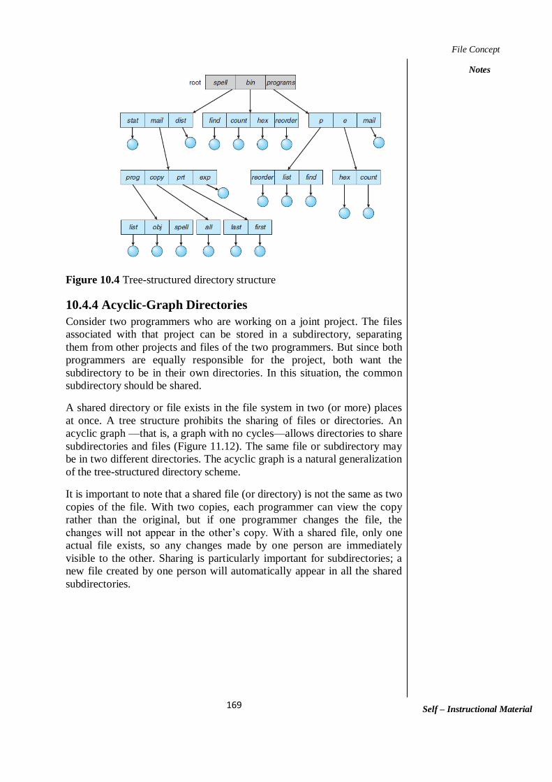
169

File Concept

Notes


Figure 10.4 Tree-structured directory structure

10.4.4 Acyclic-Graph Directories

Consider two programmers who are working on a joint project. The files

associated with that project can be stored in a subdirectory, separating

them from other projects and files of the two programmers. But since both

programmers are equally responsible for the project, both want the

subdirectory to be in their own directories. In this situation, the common

subdirectory should be shared.

A shared directory or file exists in the file system in two (or more) places

at once. A tree structure prohibits the sharing of files or directories. An

acyclic graph —that is, a graph with no cycles—allows directories to share

subdirectories and files (Figure 11.12). The same file or subdirectory may

be in two different directories. The acyclic graph is a natural generalization

of the tree-structured directory scheme.

It is important to note that a shared file (or directory) is not the same as two

copies of the file. With two copies, each programmer can view the copy

rather than the original, but if one programmer changes the file, the

changes will not appear in the other’s copy. With a shared file, only one

actual file exists, so any changes made by one person are immediately

visible to the other. Sharing is particularly important for subdirectories; a

new file created by one person will automatically appear in all the shared

subdirectories.

170

File Concept

Notes


Figure 10.5 Acyclic-graph directory structure.

10.4.5General Graph Directory

A serious problem with using an acyclic-graph structure is ensuring that

there are no cycles. If we start with a two-level directory and allow users to

create subdirectories, a tree-structured directory results. It should be fairly

easy to see that simply adding new files and subdirectories to an existing

tree-structured directory preserves the tree-structured nature. However,

when we add links, the tree structure is destroyed, resulting in a simple

graph structure (Figure 11.13). The primary advantage of an acyclic graph

is the relative simplicity of the algorithms to traverse the graph and to

determine when there are no more references to a file. We want to avoid

traversing shared sections of an acyclic graph twice, mainly for

performance reasons. If we have just searched a major shared subdirectory

for a particular file without finding it, we want to avoid searching that

subdirectory again; the second search would be a waste of time.

If cycles are allowed to exist in the directory, we likewise want to avoid

searching any component twice, for reasons of correctness as well as

performance. A poorly designed algorithm might result in an infinite loop

continually searching through the cycle and never terminating

A similar problem exists when we are trying to determine when a file can

be deleted. With acyclic-graph directory structures, a value of 0 in the

reference count means that there are no more references to the file or

directory, and the file can be deleted. However, when cycles exist, the

reference count may not be 0 even when it is no longer possible to refer to

a directory or file. This anomaly results from the possibility of self-

referencing (or a cycle) in the directory structure. In this case, we generally

need to use a garbage collection scheme to determine when the last

171

File Concept

Notes


reference has been deleted and the disk space can be reallocated. Garbage

collection involves traversing the entire file system, marking everything

that can be accessed. Then, a second pass collects everything that is not

marked onto a list of free space. (A similar marking procedure can be used

to ensure that a traversal or search will cover everything in the file system

once and only once.) Garbage collection for a disk-based file system,

however, is extremely time consuming and is thus seldom attempted.

Figure 10.6 General graph directory

Garbage collection is necessary only because of possible cycles in the

graph. Thus, an acyclic-graph structure is much easier to work with. The

difficulty is to avoid cycles as new links are added to the structure. How do

we know when a new link will complete a cycle? There are algorithms to

detect cycles in graphs; however, they are computationally expensive,

especially when the graph is on disk storage. A simpler algorithm in the

special case of directories and links is to bypass links during directory

traversal. Cycles are avoided, and no extra overhead is incurred.

Check your Progress

1. How to create a File?

2. How to write a file?

3. How to read a file?

4. How to delete a file?

5. What truncating a file?


1. Two steps are necessary to create a file. First, space in the file

system must be found for the file. We discuss how to allocate space

for the file in Chapter 12. Second, an entry for the new file must be

made in the directory.

2. To write a file, we make a system call specifying both the name of

the file and the information to be written to the file. Given the name

172

File Concept

Notes


of the file, the system searches the directory to find the file’s

location. The system must keep a write pointer to the location in the

file Self-Instructional Material NOTES 136 where the next write is

to take place. The write pointer must be updated whenever a write

occurs.

3. To read from a file, we use a system call that specifies the name of

the file and where (in memory) the next block of the file should be

put. Again, the directory is searched for the associated entry, and

the system needs to keep a read pointer to the location in the file

where the next read is to take place. Once the read has taken place,

the read pointer is updated. Because a process is usually either

reading from or writing to a file, the current operation location can

be kept as a per-process current fileposition pointer. Both the read

and write operations use this same pointer, saving space and

reducing system complexity.

4. To delete a file, we search the directory for the named file. Having

found the associated directory entry, we release all file space, so

that it can be reused by other files, and erase the directory entry.

5. The user may want to erase the contents of a file but keep its

attributes. Rather than forcing the user to delete the file and then

recreate it, this function allows all attributes to remain unchanged—

except for file length—but lets the file be reset to length zero and

its file space released

10.6. SUMMARY Files are the important storage structures in which data can be

easily stores and access.

To write a file, we make a system call specifying both the name of

the file and the information to be written to the file.

Direct-access files are of great use for immediate access to large

amounts of information. Databases are often of this type.

A shared directory or file exists in the file system in two (or more)

places at once.

A single-level directory has significant limitations, however, when

the number of files increases or when the system has more than one

user.

10.7. KEYWORDS

File: A file is a named collection of related information that is

recorded on secondary storage such as magnetic disks, magnetic

tapes and optical disks.

Sequential access: Information in the file is processed in order,

one record after the other.

173

File Concept

Notes


Directory: The directory can be viewed as a symbol table that

translates file names into their directory entries.

Single level dictionary: The simplest directory structure is the

single-level directory. All files are contained in the same directory,

which is easy to support and understand

Protection. Access-control information determines who can do

reading, writing, executing, and so on.



1. What is Sequential Access?

2. What is Direct Access?

3. What is Single Level Directory?

4. What is Two Level Directory?

5. What is Acyclic Graph Directory?


1. Explain File Operations?

2. Explain File Attributes?










174

Structures

Notes


UNIT XI STRUCTURES

Structure

11.0 Introduction

11.1Objective

11.2 File-System Mounting

11.3 File Sharing

11.4 Protection


11.6 Summary

11.7 Key Words



11.0 INTRODUCTION This unit describes the file system mounting and the various ways the file

system can be shared. Mounting is a process by which the operating

system makes files and directories on a storage device (such as hard drive,

CD-ROM, or network share) available for users to access via the

computer's file system. In general, the process of mounting comprises

operating system acquiring access to the storage medium; recognizing,

reading, processing file system structure and metadata on it; before

registering them to the virtual file system (VFS) component. The location

in VFS that the newly-mounted medium was registered is called mount

point; when the mounting process is completed, the user can access files

and directories on the medium from there. Once the file us created it also

needs to protect. The file protection method helps to safeguard the file

information and view it more protectively.

11.1 OBJECTIVE

This unit explores and helps to understand the user with the following

concepts such as

File system Mounting

File sharing

Protection

11.2 FILE-SYSTEM MOUNTING

Just as a file must be opened before it is used, a file system must be

mounted before it can be available to processes on the system. More

specifically, the directory structure may be built out of multiple volumes,

which must be mounted to make them available within the file-system

name space. The mount procedure is straightforward. The operating system

is given the name of the device and the mount point—the location within

the file structure where the file system is to be attached. Some operating

systems require that a file system type be provided, while others inspect

175

Structures

Notes


the structures of the device and determine the type of file system.

Typically, a mount point is an empty directory. For instance, on a UNIX

system, a file system containing a user’s home directories might be

mounted as /home; then, to access the directory structure within that file

system, we could precede the directory names with /home, as in

/home/jane. Mounting that file system under /users would result in the path

name /users/jane, which we could use to reach the same directory.

Next, the operating system verifies that the device contains a valid file

system. It does so by asking the device driver to read the device directory

and verifying that the directory has the expected format. Finally, the

operating system notes in its directory structure that a file system is

mounted at the specified mount point. This scheme enables the operating

system to traverse its directory structure, switching among file systems,

and even file systems of varying types, as appropriate.

Figure 11.1 File system. (a) Existing system. (b) Unmounted volume.

To illustrate file mounting, consider the file system depicted in Figure

11.14, where the triangles represent subtrees of directories that are of

interest. Figure 11.14(a) shows an existing file system, while Figure

11.14(b) shows an unmounted volume residing on /device/dsk. At this

point, only the files on the existing file system can be accessed. Figure

11.15 shows the effects of mounting the volume residing on /device/dsk

over /users. If the volume is unmounted, the file system is restored to the

situation depicted in Figure 11.14. Systems impose semantics to clarify

functionality. For example, a system may disallow a mount over a

directory that contains files; or it may make the mounted file system

available at that directory and obscure the directory’s existing files until

the file system is unmounted, terminating the use of the file system and

allowing access to the original files in that directory. As another example, a

176

Structures

Notes


system may allow the same file system to be mounted repeatedly, at

different mount points; or it may only allow one mount per file system.

Consider the actions of the Mac OS X operating system. Whenever the

system encounters a disk for the first time (either at boot time or while the

system is running), the Mac OS X operating system searches for a file

system on the device. If it finds one, it automatically mounts the file

system under m the /Volumes directory, adding a folder icon labeled with

the name of the file system (as stored in the device directory). The user is

then able to click on the icon and thus display the newly mounted file

Figure 11.2 Mount point.

The Microsoft Windows family of operating systems maintains an

extended two-level directory structure, with devices and volumes assigned

drive letters. Volumes have a general graph directory structure associated

with the drive letter. The path to a specific file takes the form of drive-

letter:\path\to\file. The more recent versions of Windows allow a file

system to be mounted anywhere in the directory tree, just as UNIX does.

Windows operating systems automatically discover all devices and mount

all located file systems at boot time. In some systems, like UNIX, the

mount commands are explicit. A system configuration file contains a list of

devices and mount points for automatic mounting at boot time, but other

mounts may be executed manually.

11.3 FILE SHARING

In this section, we examine more aspects of file sharing. We begin by

discussing general issues that arise when multiple users share files. Once

multiple users are allowed to share files, the challenge is to extend sharing

to multiple file systems, including remote file systems; we discuss that

177

Structures

Notes


challenge as well. Finally, we consider what to do about conflicting actions

occurring on shared files.

11.3.1 MULTIPLE USERS

When an operating system accommodates multiple users, the issues of file

sharing, file naming, and file protection become preeminent. Given a

directory structure that allows files to be shared by users, the system must

mediate the file sharing. The system can either allow a user to access the

files of other users by default or require that a user specifically grant access

to the files. These are the issues of access control and protection, which are

covered in Section 11.6. To implement sharing and protection, the system

must maintain more file and directory attributes than are needed on a

single-user system. Although many approaches have been taken to meet

this requirement, most systems have evolved to use the concepts of file (or

directory) owner (or user) and group. The owner is the user who can

change attributes and grant access and who has the most control over the

file. The group attribute defines a subset of users who can share access to

the file. For example, the owner of a file on a UNIX system can issue all

operations on a file, while members of the file’s group can execute one

subset of those operations, and all other users can execute another subset of

operations. Exactly which operations can be executed by group members

and other users is definable by the file’s owner. More details on permission

attributes are included in the next section.

The owner and group IDs of a given file (or directory) are stored with the

other file attributes. When a user requests an operation on a file, the user

ID can be compared with the owner attribute to determine if the requesting

user is the owner of the file. Likewise, the group IDs can be compared. The

result indicates which permissions are applicable. The system then applies

those permissions to the requested operation and allows or denies it. Many

systems have multiple local file systems, including volumes of a single

disk or multiple volumes on multiple attached disks. In these cases, the ID

checking and permission matching are straightforward, once the file

systems are mounted.

11.3.2 Remote File Systems

With the advent of networks communication among remote computers

became possible. Networking allows the sharing of resources spread across

a campus or even around the world. One obvious resource to share is data

in the form of files. Through the evolution of network and file technology,

remote file-sharing methods have changed. The first implemented method

involves manually transferring files between machines via programs like

ftp. The second major method uses a distributed file system (DFS) in

which remote directories are visible from a local machine. In some ways,

the third method, the WorldWide

Web, is a reversion to the first. A browser is needed to gain access to the

remote files, and separate operations (essentially a wrapper for ftp) are

used to transfer files. Increasingly, cloud computing is being used for file

178

Structures

Notes


sharing as well. ftp is used for both anonymous and authenticated access.

Anonymous access allows a user to transfer files without having an

account on the remote system. The WorldWideWeb uses anonymous file

exchange almost exclusively. DFS involves a much tighter integration

between the machine that is accessing the remote files and the machine

providing the files. This integration adds complexity, as we describe in this

section.

11.3.3 The Client–Server Model

Remote file systems allow a computer to mount one or more file systems

from one or more remote machines. In this case, the machine containing

the files is the server, and the machine seeking access to the files is the

client. The client–server relationship is common with networked machines.

Generally, the server declares that a resource is available to clients and

specifies exactly which resource (in this case, which files) and exactly

which clients. A server can serve multiple clients, and a client can use

multiple servers, depending on the implementation details of a given

client–server facility. The server usually specifies the available files on a

volume or directory level. Client identification is more difficult. A client

can be specified by a network name or other identifier, such as an IP

address, but these can be spoofed, or imitated. As a result of spoofing, an

unauthorized client could be allowed access to the server. More secure

solutions include secure authentication of the client via encrypted keys.

Unfortunately, with security come many challenges, including ensuring

compatibility of the client and server (they must use the same encryption

algorithms) and security of key exchanges (intercepted keys could again

allow unauthorized access). Because of the difficulty of solving these

problems, unsecure authentication methods are most commonly used.

In the case of UNIX and its network file system (NFS), authentication

takes place via the client networking information, by default. In this

scheme, the user’s IDs on the client and server must match. If they do not,

the server will be unable to determine access rights to files. Consider the

example of a user who has an ID of 1000 on the client and 2000 on the

server. A request from the client to the server for a specific file will not be

handled appropriately, as the server will determine if user 1000 has access

to the file rather than basing the determination on the real user ID of 2000.

Access is thus granted or denied based on incorrect authentication

information. The server must trust the client to present the correct user ID.

Note that the NFS protocols allow many-to-many relationships. That is,

many servers can provide files to many clients. In fact, a given machine

can be both a server to some NFS clients and a client of other NFS servers.

Once the remote file system is mounted, file operation requests are sent on

behalf of the user across the network to the server via the DFS protocol.

Typically, a file-open request is sent along with the ID of the requesting

user. The server then applies the standard access checks to determine if the

user has credentials to access the file in the mode requested. The request is

either allowed or denied. If it is allowed, a file handle is returned to the

client application, and the application then can perform read, write, and

179

Structures

Notes


other operations on the file. The client closes the file when access is

completed. The operating system may apply semantics similar to those for

a local file-system mount or may use different semantics.

11.3.4 Distributed Information Systems

To make client–server systems easier to manage, distributed information

systems, also known as distributed naming services, provide unified access

to the information needed for remote computing. The domain name system

(DNS) provides host-name-to-network-address translations for the entire

Internet. Before DNS became widespread, files containing the same

information were sent via e-mail or ftp between all networked hosts.

Obviously, this methodology was not scalable. Other distributed

information systems provide user name/password/user ID/group ID space

for a distributed facility. UNIX systems have employed a wide variety of

distributed information methods. Sun Microsystems (now part of Oracle

Corporation) introduced yellow pages (since renamed network information

service, or NIS), and most of the industry adopted its use. It centralizes

storage of user names, host names, printer information, and the like.

Unfortunately, it uses unsecure authentication methods, including sending

user passwords unencrypted (in clear text) and identifying hosts by IP

address. Sun’s NIS+ was a much more secure replacement for NIS but was

much more complicated and was not widely adopted. In the case of

Microsoft’s common Internet file system (CIFS), network information is

used in conjunction with user authentication (user name and password) to

create a network login that the server uses to decide whether to allow or

deny access to a requested file system. For this authentication to be valid,

the user names must match from machine to machine (as with NFS).

Microsoft uses active directory as a distributed naming structure to provide

a single name space for users. Once established, the distributed naming

facility is used by all clients and servers to authenticate users.

The industry is moving toward use of the lightweight directory-access

protocol (LDAP) as a secure distributed naming mechanism. In fact, active

directory is based on LDAP. Oracle Solaris and most other major operating

systems include LDAP and allow it to be employed for user authentication

as well as system-wide retrieval of information, such as availability of

printers. Conceivably, one distributed LDAP directory could be used by an

organization to store all user and resource information for all the

organization’s computers. The result would be secure single sign-on for

users, who would enter their authentication information once for access to

all computers within the organization. It would also ease system-

administration efforts by combining, in one location, information that is

currently scattered in various files on each system or in different

distributed information services.

11.3.5 Failure Modes

Local file systems can fail for a variety of reasons, including failure of the

disk containing the file system, corruption of the directory structure or

180

Structures

Notes


other disk-management information (collectively called metadata), disk-

controller failure, cable failure, and host-adapter failure. User or system-

administrator failure can also cause files to be lost or entire directories or

volumes to be deleted. Many of these failures will cause a host to crash and

an error condition to be displayed, and human intervention will be required

to repair the damage. Remote file systems have even more failure modes.

Because of the complexity of network systems and the required

interactions between remote machines, many more problems can interfere

with the proper operation of remote file systems. In the case of networks,

the network can be interrupted between two hosts. Such interruptions can

result from hardware failure, poor hardware configuration, or networking

implementation issues. Although some networks have built-in resiliency,

including multiple paths between hosts, many do not. Any single failure

can thus interrupt the flow of DFS commands.

Consider a client in the midst of using a remote file system. It has files

open from the remote host; among other activities, it may be performing

directory lookups to open files, reading or writing data to files, and closing

files. Now consider a partitioning of the network, a crash of the server, or

even a scheduled shutdown of the server. Suddenly, the remote file system

is no longer reachable. This scenario is rather common, so it would not be

appropriate for the client system to act as it would if a local file system

were lost. Rather, the system can either terminate all operations to the lost

server or delay operations until the server is again reachable. These failure

semantics are defined and implemented as part of the remote-file-system

protocol. Termination of all operations can result in users’ losing data—

and patience. Thus, most DFS protocols either enforce or allow delaying of

file-system operations to remote hosts, with the hope that the remote host

will become available again.

To implement this kind of recovery from failure, some kind of state

information may be maintained on both the client and the server. If both

server and client maintain knowledge of their current activities and open

files, then they can seamlessly recover from a failure. In the situation

where the server crashes but must recognize that it has remotely mounted

exported file systems and opened files, NFS takes a simple approach,

implementing a stateless DFS.

In essence, it assumes that a client request for a file read or write would not

have occurred unless the file system had been remotely mounted and the

file had been previously open. The NFS protocol carries all the information

needed to locate the appropriate file and perform the requested operation.

Similarly, it does not track which clients have the exported volumes

mounted, again assuming that if a request comes in, it must be legitimate.

While this stateless approach makes NFS resilient and rather easy to

implement, it also makes it unsecure. For example, forged read or write

requests could be allowed by an NFS server. These issues are addressed in

the industry standard NFS Version 4, in which NFS is made stateful to

improve its security, performance, and functionality.

181

Structures

Notes


11.3.6 Consistency Semantics

Consistency semantics represent an important criterion for evaluating any

file system that supports file sharing. These semantics specify how

multiple users of a system are to access a shared file simultaneously. In

particular, they specify when modifications of data by one user will be

observable by other users. These semantics are typically implemented as

code with the file system.

Consistency semantics are directly related to the process synchronization

algorithms of Chapter 5. However, the complex algorithms of that chapter

tend not to be implemented in the case of file I/O because of the great

latencies and slow transfer rates of disks and networks. For example,

performing an atomic transaction to a remote disk could involve several

network communications, several disk reads and writes, or both. Systems

that attempt such a full set of functionalities tend to perform poorly. A

successful implementation of complex sharing semantics can be found in

the Andrew file system. For the following discussion, we assume that a

series of file accesses (that is, reads and writes) attempted by a user to the

same file is always enclosed between the open() and close() operations.

The series of accesses between the open() and close() operations makes up

a file session. To illustrate the concept, we sketch several prominent

examples of consistency semantics.

11.3.7 Immutable-Shared-Files Semantics

A unique approach is that of immutable shared files. Once a file is declared

as shared by its creator, it cannot be modified. An immutable file has two

key properties: its name may not be reused, and its contents may not be

altered. Thus, the name of an immutable file signifies that the contents of

the file are fixed.

11.4 PROTECTION

When information is stored in a computer system, we want to keep it safe

from physical damage (the issue of reliability) and improper access (the

issue of protection). Reliability is generally provided by duplicate copies of

files. Many computers have systems programs that automatically (or

through computer-operator intervention) copy disk files to tape at regular

intervals (once per day or week or month) to maintain a copy should a file

system be accidentally destroyed.

File systems can be damaged by hardware problems (such as errors in

reading or writing), power surges or failures, head crashes, dirt,

temperature extremes, and vandalism. Files may be deleted accidentally.

Bugs in the file-system software can also cause file contents to be lost.

Reliability is covered in more detail in Chapter 10.

Protection can be provided in many ways. For a single-user laptop system,

we might provide protection by locking the computer in a desk drawer or

file cabinet. In a larger multiuser system, however, other mechanisms are

needed.

182

Structures

Notes


11.4.1 Types of Access

The need to protect files is a direct result of the ability to access files.

Systems that do not permit access to the files of other users do not need

protection. Thus, we could provide complete protection by prohibiting

access. Alternatively, we could provide free access with no protection.

Both approaches are too extreme for general use. What is needed is

controlled access. Protection mechanisms provide controlled access by

limiting the types of file access that can be made. Access is permitted or

denied depending on several factors, one of which is the type of access

requested. Several different types of operations may be controlled:

• Read. Read from the file.

• Write.Write or rewrite the file.

• Execute. Load the file into memory and execute it.

• Append.Write new information at the end of the file.

• Delete. Delete the file and free its space for possible reuse.

• List. List the name and attributes of the file.

Other operations, such as renaming, copying, and editing the file, may also

be controlled. For many systems, however, these higher-level functions

may be implemented by a system program that makes lower-level system

calls. Protection is provided at only the lower level. For instance, copying a

file maybe implemented simply by a sequence of read requests. In this

case, a user with read access can also cause the file to be copied, printed,

and so on.

Many protection mechanisms have been proposed. Each has advantages

and disadvantages and must be appropriate for its intended application. A

small computer system that is used by only a few members of a research

group, for example, may not need the same types of protection as a large

corporate computer that is used for research, finance, and personnel

operations.

11.4.2 Access Control

The most common approach to the protection problem is to make access

dependent on the identity of the user. Different users may need different

types of access to a file or directory. The most general scheme to

implement identity dependent access is to associate with each file and

directory an access-control list (ACL) specifying user names and the types

of access allowed for each user. When a user requests access to a particular

file, the operating system checks the access list associated with that file. If

that user is listed for the requested access, the access is allowed.

Otherwise, a protection violation occurs, and the user job is denied access

to the file.

183

Structures

Notes


This approach has the advantage of enabling complex access

methodologies. The main problem with access lists is their length. If we

want to allow everyone to read a file, we must list all users with read

access. This technique has two undesirable consequences:

• Constructing such a list may be a tedious and unrewarding task,

especially if we do not know in advance the list of users in the system.

• The directory entry, previously of fixed size, now must be of variable

size, resulting in more complicated space management.

These problems can be resolved by use of a condensed version of the

access list. To condense the length of the access-control list, many systems

recognize three classifications of users in connection with each file:

• Owner. The user who created the file is the owner.

• Group. A set of users who are sharing the file and need similar access is a

group, or work group.

• Universe. All other users in the system constitute the universe.

The most common recent approach is to combine access-control lists with

the more general (and easier to implement) owner, group, and universe

access control scheme just described. For example, Solaris uses the three

categories of access by default but allows access-control lists to be added

to specific files and directories when more fine-grained access control is

desired. To illustrate, consider a person, Sara, who is writing a new book.

She has hired three graduate students (Jim, Dawn, and Jill) to help with the

project. The text of the book is kept in a file named book.tex. The

protection associated with this file is as follows:

• Sara should be able to invoke all operations on the file.

• Jim, Dawn, and Jill should be able only to read and write the file; they

should not be allowed to delete the file.

184

Structures

Notes


Figure11.3 windows 7 access control

• All other users should be able to read, but not write, the file. (Sara is

interested in letting as many people as possible read the text so that she can

obtain feedback.)

To achieve such protection, we must create a new group—say, text— with

members Jim, Dawn, and Jill. The name of the group, text, must then be

associated with the file book.tex, and the access rights must be set in

accordance with the policy we have outlined. Now consider a visitor to

whom Sara would like to grant temporary access to Chapter 1. The visitor

cannot be added to the text group because that would give him access to all

chapters. Because a file can be in only one group.

Check your Progress

1. What is Access Control?

2. What is Read, Write and Execute access?

3. What is Immutable-Shared-Files Semantics?

4. What is a client and server?

5. What is Remote File System?


1. The goal of access control is to minimize the risk of

unauthorized access to physical and logical systems. Access

control is a fundamental component of security compliance

programs that ensures security technology and access

control policies are in place to protect confidential information,

such as customer data.

2. Read. Read from the file.

Write.Write or rewrite the file.

Execute. Load the file into memory and execute it.

3. When a file is declared as shared by its creator, it

becomes immutable and the name cannot be re-used for any other

resource. Hence it becomes read-only, and shared access is simple.

4. The machine containing the files is the server, and the machine

seeking access to the files is the client.

5. The RFS (Remote File System) is a file system that allows the user

to "share" a directory on a PC with remote PC over a serial

connection. Remote PC will be able to access files on the shared

PC directory just as they were local files; they can be opened, read,

written, closed and so on.

185

Structures

Notes


11.6. SUMMARY Once multiple users are allowed to share files, the challenge is

to extend sharing to multiple file systems, including remote file

systems

Networking allows the sharing of resources spread across a

campus or even around the world.

Remote file systems allow a computer to mount one or more

file systems from one or more remote machines.

Local file systems can fail for a variety of reasons, including

failure of the disk containing the file system, corruption of the

directory structure or other disk-management information, and

so on.

The most common approach to the protection problem is to

make access dependent on the identity of the user.

11.7. KEYWORDS

Distributed information system: To make client–server systems

easier to manage, distributed information systems, also known as

distributed naming services, provide unified access to the

information needed for remote computing.

DNS: The domain name system (DNS) provides host-name-to-

network-address translations for the entire Internet.

Consistency semantics: Consistency semantics represent an

important criterion for evaluating any file system that supports file

sharing.



1. What is Client server model?

2. What is Distributed Information system?

3. What is Failure modes?

4. What is Consistency Semantics?

5. What are types of Access?


1. Explain File System Mounting?

2. Explain File Sharing?

3. Explain Protection?

186

Structures

Notes











187

Implementing File Systems

Notes


UNIT XII

IMPLEMENTING FILE SYSTEMS

Structure

12.0 Introduction

12.1 Objectives

12.2 File-System Structure

12.3 File-System Implementation


12.5 Summary

12.6 Key Words



12.0 INTRODUCTION

This unit briefs the file system implementation and how it is structured.

Disks offer the massive amount of secondary storage where a file system

can be maintained. They have two characteristics which make them a

suitable medium for storing various files. A disk can be used to rewrite in

place; it is possible to read a chunk from the disk, modify the chunk and

write it back there in the same place. A disk can access directly any given

block of data it contains. Hence, it is easy to access any file either in

sequence or at random and switching from one single file to another need

only to move the read-write heads and wait for the disk to rotate to that

specific location. This also explains the free space management on how the

files can be allocated and retrieved. The file system basic operations and

implementation are illustrated.

12.1 OBJECTIVES

The user can understand the following concepts when they go through this

unit such as

Structure of the File system

Implementation of file system

12.2 FILE-SYSTEM STRUCTURE

Disks provide most of the secondary storage on which file systems are

maintained. Two characteristics make them convenient for this purpose:

1. A disk can be rewritten in place; it is possible to read a block from the

disk, modify the block, and write it back into the same place.

188


Notes


2. A disk can access directly any block of information it contains. Thus, it

is simple to access any file either sequentially or randomly, and switching

from one file to another requires only moving the read–write heads and

waiting for the disk to rotate.

To improve I/O efficiency, I/O transfers between memory and disk are

performed in units of blocks. Each block has one or more sectors.

Depending on the disk drive, sector size varies from 32 bytes to 4,096

bytes; the usual size is 512 bytes.

Figure12.1 Layered Structure

File systems provide efficient and convenient access to the disk by

allowing data to be stored, located, and retrieved easily. A file system

poses two quite different design problems. The first problem is defining

how the file system should look to the user. This task involves defining a

file and its attributes, the operations allowed on a file, and the directory

structure for organizing files. The second problem is creating algorithms

and data structures to map the logical file system onto the physical

secondary-storage devices. The file system itself is generally composed of

many different levels. The structure shown in Figure 12.1 is an example of

a layered design. Each level in the design uses the features of lower levels

to create new features for use by higher levels.

The I/O control level consists of device drivers and interrupt handlers to

transfer information between the main memory and the disk system. A

device driver can be thought of as a translator. Its input consists of high-

level commands such as ―retrieve block 123.‖ Its output consists of low-

level, hardware-specific instructions that are used by the hardware

controller, which interfaces the I/O device to the rest of the system. The

device driver usually writes specific bit patterns to special locations in the

189


Notes


I/O controller’s memory to tell the controller which device location to act

on and what actions to take.

The basic file system needs only to issue generic commands to the

appropriate device driver to read and write physical blocks on the disk.

Each physical block is identified by its numeric disk address (for example,

drive 1, cylinder 73, track 2, sector 10). This layer also manages the

memory buffers and caches that hold various file-system, directory, and

data blocks. A block in the buffer is allocated before the transfer of a disk

block can occur. When the buffer is full, the buffer manager must find

more buffer memory or free up buffer space to allow a requested I/O to

complete. Caches are used to hold frequently used file-system metadata to

improve performance, so managing their contents is critical for optimum

system performance.

The file-organization module knows about files and their logical blocks, as

well as physical blocks. By knowing the type of file allocation used and the

location of the file, the file-organization module can translate logical block

addresses to physical block addresses for the basic file system to transfer.

Each file’s logical blocks are numbered from 0 (or 1) through N. Since the

physical blocks containing the data usually do not match the logical

numbers, a translation is needed to locate each block.

The file-organization module also includes the free-space manager, which

tracks unallocated blocks and provides these blocks to the file-organization

module when requested. Finally, the logical file system manages metadata

information. Metadata includes all of the file-system structure except the

actual data (or contents of the files). The logical file system manages the

directory structure to provide the file-organization module with the

information the latter needs, given a symbolic file name. It maintains file

structure via file-control blocks. A file control block (FCB) (an inode in

UNIX file systems) contains information about the file, including

ownership, permissions, and location of the file contents.

When a layered structure is used for file-system implementation,

duplication of code is minimized. The I/O control and sometimes the basic

file-system code can be used by multiple file systems. Each file system can

then have its own logical file-system and file-organization modules.

Unfortunately, layering can introduce more operating-system overhead,

which may result in decreased performance. The use of layering, including

the decision about how many layers to use and what each layer should do,

is a major challenge in designing new systems.

Many file systems are in use today, and most operating systems support

more than one. For example, most CD-ROMs are written in the ISO 9660

format, a standard format agreed on by CD-ROM manufacturers. In

addition to removable-media file systems, each operating system has one

or more disk based file systems. UNIX uses the UNIX file system (UFS),

which is based on the Berkeley Fast File System (FFS). Windows supports

disk file-system formats of FAT, FAT32, and NTFS (or Windows NT File

System), as well as CD-ROM and DVD file-system formats. Although

190


Notes


Linux supports over forty different file systems, the standard Linux file

system is known as the extended file system, with the most common

versions being ext3 and ext4. There are also distributed file systems in

which a file system on a server is mounted by one or more client

computers across a network.

File-system research continues to be an active area of operating-system

design and implementation. Google created its own file system to meet the

company’s specific storage and retrieval needs, which include high

performance access from many clients across a very large number of disks.

Another interesting project is the FUSE file system, which provides

flexibility in file-system development and use by implementing and

executing file systems as user-level rather than kernel-level code. Using

FUSE, a user can add a new file system to a variety of operating systems

and can use that file system to manage her files.

12.3 FILE-SYSTEM IMPLEMENTATION

As was described in Section 11.1.2, operating systems implement open()

and close() systems calls for processes to request access to file contents. In

this section, we delve into the structures and operations used to implement

file-system operations.

12.3.1 Overview

Several on-disk and in-memory structures are used to implement a file

system. These structures vary depending on the operating system and the

file system, but some general principles apply. On disk, the file system

may contain information about how to boot an operating system stored

there, the total number of blocks, the number and location of free blocks,

the directory structure, and individual files. Many of these structures are

detailed throughout the remainder of this chapter. Here, we describe them

briefly:

• A boot control block (per volume) can contain information needed by the

system to boot an operating system from that volume. If the disk does not

contain an operating system, this block can be empty. It is typically the

first block of a volume. In UFS, it is called the boot block. In NTFS, it is

the partition boot sector.

• A volume control block (per volume) contains volume (or partition)

details, such as the number of blocks in the partition, the size of the blocks,

a free-block count and free-block pointers, and a free-FCB count and FCB

pointers. In UFS, this is called a superblock. In NTFS, it is stored in the

master file table.

• A directory structure (per file system) is used to organize the files. In

UFS, this includes file names and associated in node numbers. In NTFS, it

is stored in the master file table.

• A per-file FCB contains many details about the file. It has a unique

identifier number to allow association with a directory entry. In NTFS, this

191


Notes


information is actually stored within the master file table, which uses a

relational database structure, with a row per file.

The in-memory information is used for both file-system management and

performance improvement via caching. The data are loaded at mount time,

updated during file-system operations, and discarded at dismount. Several

types of structures may be included.

• An in-memory mount table contains information about each mounted

volume.

• An in-memory directory-structure cache holds the directory information

of recently accessed directories. (For directories at which volumes are

mounted, it can contain a pointer to the volume table.)

• The system-wide open-file table contains a copy of the FCB of each open

file, as well as other

The per-process open-file table contains a pointer to the appropriate entry

in the system-wide open-file table, as well as other information.

• Buffers hold file-system blocks when they are being read from disk or

written to disk.

To create a new file, an application program calls the logical file system.

The logical file system knows the format of the directory structures. To

create a new file, it allocates a new FCB. (Alternatively, if the file-system

implementation creates all FCBs at file-system creation time, an FCB is

allocated from the set of free FCBs.) The system then reads the appropriate

directory into memory, updates it with the new file name and FCB, and

writes it back to the disk. Atypical FCB is shown in Figure 12.2.

12.3.2 Partitions and Mounting

The layout of a disk can have many variations, depending on the operating

system. A disk can be sliced into multiple partitions, or a volume can span

multiple partitions on multiple disks. Each partition can be either ―raw,‖

containing no file system, or ―cooked,‖ containing a file system. Raw disk

is used where no file system is appropriate. UNIX swap space can use a

raw partition, for example, since it uses its own format on disk and does

not use a file system. Likewise, some databases use raw disk and format

the data to suit their needs. Raw disk can also hold information needed by

disk RAID systems, such as bit maps indicating which blocks are mirrored

and which have changed and need to be mirrored. Similarly, raw disk can

contain a miniature database holding RAID configuration information,

such as which disks are members of each RAID set. Raw disk use is

discussed in Section 10.5.1.

Boot information can be stored in a separate partition, as described in

Section 10.5.2. Again, it has its own format, because at boot time the

system does not have the file-system code loaded and therefore cannot

interpret the file-system format. Rather, boot information is usually a

192


Notes


sequential series of blocks, loaded as an image into memory. Execution of

the image starts at a predefined location, such as the first byte. This boot

loader in turn knows enough about the file-system structure to be able to

find and load the kernel and start it executing.

It can contain more than the instructions for how to boot a specific

operating system. For instance, many systems can be dual-booted, allowing

us to install multiple operating systems on a single system. How does the

system know which one to boot? A boot loader that understands multiple

file systems and multiple operating systems can occupy the boot space.

Once loaded, it can boot one of the operating systems available on the disk.

The disk can have multiple partitions, each containing a different type of

file system and a different operating system.

The root partition, which contains the operating-system kernel and

sometimes other system files, is mounted at boot time. Other volumes can

be automatically mounted at boot or manually mounted later, depending on

the operating system. As part of a successful mount operation, the

operating system verifies that the device contains a valid file system. It

does so by asking the device driver to read the device directory and

verifying that the directory has the expected format. If the format is

invalid, the partition must have its consistency checked and possibly

corrected, either with or without user intervention. Finally, the operating

system notes in its in-memory mount table that a file system is mounted,

along with the type of the file system. The details of this function depend

on the operating system.

193


Notes


Figure12.2 in memory file structures

Microsoft Windows–based systems mount each volume in a separate name

space, denoted by a letter and a colon. To record that a file system is

mounted at F:, for example, the operating system places a pointer to the

file system in a field of the device structure corresponding to F:. When a

process specifies the driver letter, the operating system finds the

appropriate file-system pointe rand traverses the directory structures on

that device to find the specified file or directory. Later versions of

Windows can mount a file system at any point within the existing directory

structure.

On UNIX, file systems can be mounted at any directory. Mounting is

implemented by setting a flag in the in-memory copy of the inode for that

directory. The flag indicates that the directory is a mount point. A field

then points to an entry in the mount table, indicating which device is

mounted there. The mount table entry contains a pointer to the superblock

of the file system on that device. This scheme enables the operating system

to traverse its directory structure, switching seamlessly among file systems

of varying types.

12.3.3 Virtual File Systems

The previous section makes it clear that modern operating systems must

concurrently support multiple types of file systems. But how does an

operating system allow multiple types of file systems to be integrated into

a directory structure? And how can users seamlessly move between file-

system types as they navigate the file-system space? We now discuss some

of these implementation details. An obvious but suboptimal method of

implementing multiple types of file systems is to write directory and file

routines for each type. Instead, however, most operating systems, including

UNIX, use object-oriented techniques to simplify, organize, and

modularize the implementation. The use of these methods allows very

dissimilar file-system types to be implemented within the same structure,

including network file systems, such as NFS. Users can access files

contained within multiple file systems on the local disk or even on file

systems available across the network.

Data structures and procedures are used to isolate the basic system call

functionality from the implementation details. Thus, the file-system

implementation consists of three major layers, as depicted schematically in

Figure 12.4. The first layer is the file-system interface, based on the open(),

read(), write(), and close() calls and on file descriptors. The second layer is

called the virtual file system (VFS) layer. The VFS layer serves two

important functions:

1. It separates file-system-generic operations from their implementation by

defining a clean VFS interface. Several implementations for the VFS

interface may coexist on the same machine, allowing transparent access to

different types of file systems mounted locally.

194


Notes


2. It provides a mechanism for uniquely representing a file throughout a

network. The VFS is based on a file-representation structure, called a

vnode, that contains a numerical designator for a network-wide unique file.

(UNIX inodes are unique within only a single file system.) This network-

wide uniqueness is required for support of network file systems.

Figure12.3 view of virtual Files

The kernel maintains one vnode structure for each active node (file or

directory). Thus, the VFS distinguishes local files from remote ones, and

local files are further distinguished according to their file-system types.

Check your Progress

1. What is a File System?

2. What is a boot control block?

3. What is a Volume control block?

4. What is a directory?

5. What is a directory structure?


1. A file system or file system (often abbreviated to fs), controls how

data is stored and retrieved. Without a file system, information

placed in a storage medium would be one large body of data with

no way to tell where one piece of information stops and the next

begins.

2. A boot control block (per volume) can contain information needed

by the system to boot an operating system from that volume. If the

disk does not contain an operating system, this block can be empty.

It is typically the first block of a volume. In UFS, it is called the

boot block. In NTFS, it is the partition boot sector.

195


Notes


3. A volume control block (per volume) contains volume (or partition)

details, such as the number of blocks in the partition, the size of the

blocks, a free-block count and free-block pointers, and a free-FCB

count and FCB pointers. In UFS, this is called a superblock. In

NTFS, it is stored in the master file table.

4. A directory is a file system cataloging structure which contains

references to other computer files, and possibly other directories.

On many computers, directories are known as folders, or drawers,

analogous to a workbench or the traditional office filing cabinet.

5. The directory structure is the organization of files into a hierarchy

of folders. Computers have used the folder metaphor for decades as

a way to help users keep track of where something can be found.

12.5. SUMMARY A disk can access directly any block of information it

contains. Thus, it is simple to access any file either

sequentially or randomly, and switching from one file to

another requires only moving the read–write heads and

waiting for the disk to rotate.

The I/O control level consists of device drivers and interrupt

handlers to transfer information between the main memory

and the disk system.

The basic file system needs only to issue generic commands

to the appropriate device driver to read and write physical

blocks on the disk.

A disk can be sliced into multiple partitions, or a volume

can span multiple partitions on multiple disks.

Data structures and procedures are used to isolate the basic

system call functionality from the implementation details.

12.6. KEYWORDS

Directory structure: It is used to organize the files. In UFS, this

includes file names and associated in node numbers. In NTFS, it is

stored in the master file table.

In-memory directory-structure: The cache holds the directory

information of recently accessed directories. (For directories at

which volumes are mounted, it can contain a pointer to the volume

table.)

VFS: The VFS is based on a file-representation structure, called a

vnode, that contains a numerical designator for a network-wide

unique file.

Booting: Boot information is usually a sequential series of blocks,

loaded as an image into memory.

196


Notes




1. What is a disk?

2. What is the purpose of the disk?

3. What are partitions?

4. What is mounting?

5. What is VFS?


1. Explain File system structure?

2. Explain File System Implementation?










197


Notes


UNIT XIII

IMPLEMENTING FILE SYSTEMS

Structure

13.0 Introduction

13.1 Objective

13.2 Directory Implementation

13.3 Allocation Methods

13.4 Free-Space Management


13.6 Summary

13.7 Key Words



13.0 INTRODUCTION

This unit explains the implementation of directories and the methods in

which means they can be accessed and the free space management

allocation are illustrated. There is the number of algorithms by using

which, the directories can be implemented. However, the selection of an

appropriate directory implementation algorithm may significantly affect

the performance of the system. The directory implementation algorithms

are classified according to the data structure they are using. The directories

path and access method are explained with the different types of allocation

methods.

13.1 OBJECTIVE

This unit covers the following

Understand the implementation of directories

Learn free space management

Study the allocation methods

13.2 DIRECTORY IMPLEMENTATION

The selection of directory-allocation and directory-management algorithms

significantly affects the efficiency, performance, and reliability of the file

system. In this section, we discuss the trade-offs involved in choosing one

of these algorithms.

13.2.1 Linear List

The simplest method of implementing a directory is to use a linear list of

file names with pointers to the data blocks. This method is simple to

program but time-consuming to execute. To create a new file, we must first

search the directory to be sure that no existing file has the same name.

198


Notes


Then, we add a new entry at the end of the directory. To delete a file,we

search the directory for the named file and then release the space allocated

to it. To reuse the directory entry, we can do one of several things. We can

mark the entry as unused (by assigning it a special name, such as an all-

blank name, or by including a used– unused bit in each entry), or we can

attach it to a list of free directory entries. A third alternative is to copy the

last entry in the directory into the freed location and to decrease the length

of the directory. A linked list can also be used to decrease the time required

to delete a file.

The real disadvantage of a linear list of directory entries is that finding a

file requires a linear search. Directory information is used frequently, and

users will notice if access to it is slow. In fact, many operating systems

implement a software cache to store the most recently used directory

information. A cache hit avoids the need to constantly reread the

information from disk. A sorted list allows a binary search and decreases

the average search time. However, the requirement that the list be kept

sorted may complicate creating and deleting files, since we may have to

move substantial amounts of directory information to maintain a sorted

directory. A more sophisticated tree data structure, such as a balanced tree,

might help here. An advantage of the sorted list is that a sorted directory

listing can be produced without a separate sort step.

13.2.1 Hash Table

Another data structure used for a file directory is a hash table. Here, a

linear list stores the directory entries, but a hash data structure is also used.

The hash table takes a value computed from the file name and returns a

pointer to the file name in the linear list. Therefore, it can greatly decrease

the directory search time. Insertion and deletion are also fairly

straightforward, although some provision must be made for collisions—

situations in which two file names hash to the same location. The major

difficulties with a hash table are its generally fixed size and the dependence

of the hash function on that size. For example, assume that we make a

linear-probing hash table that holds 64 entries. The hash function converts

file names into integers from 0 to 63 (for instance, by using the remainder

of a division by 64). If we later try to create a 65th file, we must enlarge

the directory hash table—say, to 128 entries. As a result, we need a new

hash function that must map file names to the range 0 to 127, and we must

reorganize the existing directory entries to reflect their new hash-function

values.

Alternatively, we can use a chained-overflow hash table. Each hash entry

can be a linked list instead of an individual value, and we can resolve

collisions by adding the new entry to the linked list. Lookups may be

somewhat slowed, because searching for a name might require stepping

through a linked list of colliding table entries. Still, this method is likely to

be much faster than a linear each through the entire directory.

199


Notes


13.3 ALLOCATION METHODS

The direct-access nature of disks gives us flexibility in the implementation

of files. In almost every case, many files are stored on the same disk. The

main problem is how to allocate space to these files so that disk space is

utilized effectively and files can be accessed quickly. Three major methods

of allocating disk space are in wide use: contiguous, linked, and indexed.

Each method has advantages and disadvantages. Although some systems

support all three, it is more common for a system to use one method for all

files within a file-system type.

13.3.1 Contiguous Allocation

Contiguous allocation requires that each file occupy a set of contiguous

blocks on the disk. Disk addresses define a linear ordering on the disk.

With this ordering, assuming that only one job is accessing the disk,

accessing block b +1 after block b normally requires no head movement.

When head movement is needed (from the last sector of one cylinder to the

first sector of the next cylinder), the head need only move from one track

to the next. Thus, the number of disk seeks required for accessing

contiguously allocated files is minimal, as is seek time when a seek is

finally needed. Contiguous allocation of a file is defined by the disk

address and length (in block units) of the first block. If the file is n blocks

long and starts at location b, then it occupies blocks b, b + 1, b + 2, ..., b +

n − 1. The directory entry for each file indicates the address of the starting

block and the length of the area allocated for this file (Figure 12.5).

Figure 13.1 Contiguous Memory Allocation

Accessing a file that has been allocated contiguously is easy. For

sequential access, the file system remembers the disk address of the last

block referenced and, when necessary, reads the next block. For direct

200


Notes


access to block i of a file that starts at block b, we can immediately access

block b + i. Thus, both sequential and direct access can be supported by

contiguous allocation.

Figure13.2 Index Allocation

13.3.2 Linked Allocation

Linked allocation solves all problems of contiguous allocation. With linked

allocation, each file is a linked list of disk blocks; the disk blocks may be

scattered anywhere on the disk. The directory contains a pointer to the first

and last blocks of the file. For example, a file of five blocks might start at

block 9 and continue at block 16, then block 1, then block 10, and finally

block 25 (Figure 12.6). Each block contains a pointer to the next block.

These pointers

are not made available to the user. Thus, if each block is 512 bytes in size,

and a disk address (the pointer) requires 4 bytes, then the user sees blocks

of 508 bytes. To create a new file, we simply create a new entry in the

directory. With linked allocation, each directory entry has a pointer to the

first disk block of the file. This pointer is initialized to null (the end-of-list

pointer value) to signify an empty file. The size field is also set to 0. A

write to the file causes the free-space management system to find a free

block, and this new block is written to and is linked to the end of the file.

To read a file, we simply read blocks by following the pointers from block

to block. There is no external fragmentation with linked allocation, and any

free block on the free-space list can be used to satisfy a request. The size of

a file need not be declared when the file is created. A file can continue to

grow as long as free blocks are available. Consequently, it is never

necessary to compact disk space

201


Notes


13.3.3 Indexed Allocation

Linked allocation solves the external-fragmentation and size-declaration

problems of contiguous allocation. However, in the absence of a FAT,

linked allocation cannot support efficient direct access, since the pointers

to the blocks are scattered with the blocks themselves all over the disk and

must be retrieved in order. Indexed allocation solves this problem by

bringing all the pointers together into one location: the index block. Each

file has its own index block, which is an array of disk-block addresses. The

ith entry in the index block points to the ith block of the file. The directory

contains the address of the index block (Figure 12.8). To find and read the

ith block, we use the pointer in the ith index-block entry. This scheme is

similar to the paging scheme described in Section 8.5. When the file is

created, all pointers in the index block are set to null. When the ith block is

first written, a block is obtained from the free-space manager, and its

address is put in the ith index-block entry. Indexed allocation supports

direct access, without suffering from external fragmentation, because any

free block on the disk can satisfy a request for more space. Indexed

allocation does suffer from wasted space, however. The pointer overhead

of the index block is generally greater than the pointer overhead of linked

allocation. Consider a common case in which we have a file of only one or

two blocks. With linked allocation, we lose the space of only one pointer

per block. With indexed allocation, an entire index block must be

allocated, even if only one or two pointers will be non-null.

Figure 13.3 File Allocation Table

202


Notes


13.4 FREE-SPACE MANAGEMENT

Since disk space is limited, we need to reuse the space from deleted files

for new files, if possible. (Write-once optical disks allow only one write to

any given sector, and thus reuse is not physically possible.) To keep track

of free disk space, the system maintains a free-space list. The free-space

list records all free disk blocks—those not allocated to some file or

directory. To create a file, we search the free-space list for the required

amount of space and allocate that space to the new file. This space is then

removed from the free-space list. When a file is deleted, its disk space is

added to the free-space list. The free-space list, despite its name, may not

be implemented as a list, as we discuss next.

13.4.1 Bit Vector

Frequently, the free-space list is implemented as a bit map or bit vector.

Each block is represented by 1 bit. If the block is free, the bit is 1; if the

block is allocated, the bit is 0. For example, consider a disk where blocks

2, 3, 4, 5, 8, 9, 10, 11, 12, 13, 17, 18, 25, 26, and 27 are free and the rest of

the blocks are allocated. The free-space bit map would be

001111001111110001100000011100000 ...

The main advantage of this approach is its relative simplicity and its

efficiency in finding the first free block or n consecutive free blocks on the

disk. Indeed, many computers supply bit-manipulation instructions that can

be used effectively for that purpose. One technique for finding the first free

block on a system that uses a bit-vector to allocate disk space is to

sequentially check each word in the bit map to see whether that value is not

0, since a 562 0-valued word contains only 0 bits and represents a set of

allocated blocks. The first non-0 word is scanned for the first 1 bit, which

is the location of the first free block. The calculation of the block number

is(number of bits per word) × (number of 0-value words) + offset of first 1

bit.

Again, we see hardware features driving software functionality.

Unfortunately, bit vectors are inefficient unless the entire vector is kept in

main memory (and is written to disk occasionally for recovery needs).

Keeping it in main memory is possible for smaller disks but not necessarily

for larger ones. A 1.3-GB disk with 512-byte blocks would need a bit map

of over 332 KB to track its free blocks, although clustering the blocks in

groups of four reduces this number to around 83 KB per disk. A1-TB disk

with 4-KB blocks requires 256 MB to store its bit map. Given that disk

size constantly increases, the problem with bit vectors will continue to

escalate as well.

13.4.2 Linked List

Another approach to free-space management is to link together all the free

disk blocks, keeping a pointer to the first free block in a special location on

the disk and caching it in memory. This first block contains a pointer to the

next free disk block, and so on. Recall our earlier example (Section

203


Notes


12.5.1), in which blocks 2, 3, 4, 5, 8, 9, 10, 11, 12, 13, 17, 18, 25, 26, and

27 were free and the rest of the blocks were allocated. In this situation, we

would keep a pointer to block 2 as the first free block. Block 2 would

contain a pointer to block 3, which would point to block 4, which would

point to block 5, which would point to block 8, and so on (Figure 12.10).

This scheme is not efficient; to traverse the list, we must read each block,

which requires substantial I/O time. Fortunately, however, traversing the

free list is not a frequent action. Usually, the operating system simply

needs a free block so that it can allocate that block to a file, so the first

block in the free list is used. The FAT method incorporates free-block

accounting into the allocation data structure. No separate method is

needed.

13.4.3 Grouping

A modification of the free-list approach stores the addresses of n free

blocks in the first free block. The first n−1 of these blocks are actually free.

The last block contains the addresses of another n free blocks, and so on.

The addresses of a large number of free blocks can now be found quickly,

unlike the situation when the standard linked-list approach is used.

13.4.4 Counting

Another approach takes advantage of the fact that, generally, several

contiguous blocks may be allocated or freed simultaneously, particularly

when space is allocated with the contiguous-allocation algorithm or

through clustering. Thus, rather than keeping a list of n free disk addresses,

we can keep the address of the first free block and the number (n) of free

contiguous blocks that follow the first block. Each entry in the free-space

list then consists of a disk address and a count. Although each entry

requires more space than would a simple disk address, the overall list is

shorter, as long as the count is generally greater than 1. Note that this

method of tracking free space is similar to the extent method of allocating

blocks. These entries can be stored in a balanced tree, rather than a linked

list, for efficient lookup, insertion, and deletion.

204


Notes


Figure13.4 Linked Free space

13.4.5 Space Maps

Oracle’s ZFS file system (found in Solaris and other operating systems)

was designed to encompass huge numbers of files, directories, and even

file systems (in ZFS, we can create file-system hierarchies). On these

scales, metadata I/O can have a large performance impact. Consider, for

example, that if the free-space list is implemented as a bit map, bit maps

must be modified both when blocks are allocated and when they are freed.

Freeing 1 GB of data on a 1-TB disk could cause thousands of blocks of bit

maps to be updated, because those data blocks could be scattered over the

entire disk. Clearly, the data structures for such a system could be large

and inefficient.

In its management of free space, ZFS uses a combination of techniques to

control the size of data structures and minimize the I/O needed to manage

those structures. First, ZFS creates metaslabs to divide the space on the

device into chunks of manageable size. A given volume may contain

hundreds of metaslabs. Each metaslab has an associated space map. ZFS

uses the counting algorithm to store information about free blocks. Rather

than write counting structures to disk, it uses log-structured file-system

techniques to record them. The space map is a log of all block activity

(allocating and freeing), in time order, in counting format. When ZFS

205


Notes


decides to allocate or free space from a metaslab, it loads the associated

space map into memory in a balanced-tree structure (for very efficient

operation), indexed by offset, and replays the log into that structure. The

in-memory spacemap is then an accurate representation of the allocated

and free space in the metaslab. ZFS also condenses the map as much as

possible by combining contiguous free blocks into a single entry.

Finally, the free-space list is updated on disk as part of the transaction-

oriented operations of ZFS. During the collection and sorting phase, block

requests can still occur, and ZFS satisfies these requests from the log. In

essence, the log plus the balanced tree is the free list.

Check your Progress

1. What is a bit vector?

2. What is Grouping?

3. What is Space Maps?

4. Name the Allocation methods?

5. What is Hash table?


1. A bit vector is a vector in which each element is a bit (so its value

is either 0 or 1). In most vectors, each element has a different

address in memory and can be manipulated separately from the

other elements, but we also hope to be able to perform ―vector

operations‖ that treat all elements uniformly.

2. A modification of the free-list approach stores the addresses of n

free blocks in the first free block. The first n−1 of these blocks are

actually free. The last block contains the addresses of another n free

blocks, and so on.

3. Oracle’s ZFS file system (found in Solaris and other operating

systems) was designed to encompass huge numbers of files,

directories, and even file systems (in ZFS, we can create file-

system hierarchies).

4. Contiguous Allocation, Linked Allocation and Indexed Allocation.

5. A hash table (hash map) is a data structure that implements an

associative array abstract data type, a structure that can map keys to

values. A hash table uses a hash function to compute an index into

an array of buckets or slots, from which the desired value can be

found.

13.6. SUMMARY

The simplest method of implementing a directory is to use a

linear list of file names with pointers to the data blocks.

Three major methods of allocating disk space are in wide use:

contiguous, linked, and indexed.

206


Notes


Contiguous allocation requires that each file occupy a set of

contiguous blocks on the disk.

Linked allocation solves all problems of contiguous allocation.

With linked allocation, each file is a linked list of disk blocks; the

disk blocks may be scattered anywhere on the disk.

Since disk space is limited, we need to reuse the space from

deleted files for new files, if possible.

For sequential access, the file system remembers the disk address of

the last block referenced and, when necessary, reads the next block.

13.7. KEYWORDS

ZFS: ZFS uses a combination of techniques to control the size of

data structures and minimize the I/O needed to manage those

structures.

Linked list: Another approach to free-space management is to link

together all the free disk blocks, keeping a pointer to the first free

block in a special location on the disk and caching it in memory.

Linked allocation: Linked allocation solves all problems of

contiguous allocation. With linked allocation, each file is a linked

list of disk blocks; the disk blocks may be scattered anywhere on

the disk.


EXERCISES


1. What is Linear List?

2. What is Contiguous Allocation?

3. What is Linked Allocation?

4. What is Indexed Allocation?

5. What is Linked List?


1. Explain free space management?

2. Explain Allocation methods?

3. Explain Directory Implementation?






207


Notes






208

Secondary Storage Structure

Notes


UNIT XIV

SECONDARY STORAGE STRUCTURE

Structure 14.0Introduction

14.1Objective

14.2 Overview of Mass-Storage Structure

14.3 Disk Structure

14.4 Disk Attachment

14.5 Overview of Mass-Storage Structure-Disk Attachment-Disk

Scheduling-Disk Management

14.6 Disk Management


14.8 Summary

14.9 Key Words



14.0 INTRODUCTION

The storage structure helps to store the data from the Operating System to

the system. There are many storage devices; this unit covers the secondary

storage structure on how the data is stored and retrieved. As we know, a

process needs two types of time, CPU time and IO time. For I/O, it

requests the Operating system to access the disk. However, the operating

system must be fair enough to satisfy each request and at the same time,

operating system must maintain the efficiency and speed of process

execution. The technique that operating system uses to determine the

request which is to be satisfied next is called disk scheduling. The disk

scheduling and disk management on the devices are explored.

14.1 OBJECTIVE

This unit helps the user to learn and understand the

Disk Scheduling

Disk Management

Overview of storage structures

14.2 OVERVIEW OF MASS-STORAGE STRUCTURE

In this section, we present a general overview of the physical structure of

secondary and tertiary storage devices.

209


Notes


14.2.1 Magnetic Disks

Magnetic disks provide the bulk of secondary storage for modern computer

systems. Conceptually, disks are relatively simple. Each disk platter has a

flat circular shape, like a CD. Common platter diameters range from 1.8 to

3.5 inches. The two surfaces of a platter are covered with a magnetic

material. We store information by recording it magnetically on the platters.

A read–write head ―flies‖ just above each surface of every platter. The

heads are attached to a disk arm that moves all the heads as a unit. The

surface of a platter is logically divided into circular tracks, which are

subdivided into sectors. The set of tracks that are at one arm position

makes up a cylinder. There may be thousands of concentric cylinders in a

disk drive, and each track may contain hundreds of sectors. The storage

capacity of common disk drives is measured in gigabytes.

When the disk is in use, a drive motor spins it at high speed. Most drives

rotate 60 to 250 times per second, specified in terms of rotations per

minute (RPM). Common drives spin at 5,400, 7,200, 10,000, and 15,000

RPM. Disk speed has two parts. The transfer rate is the rate at which data

flow between the drive and the computer. The positioning time, or random-

access time, consists of two parts: the time necessary to move the disk arm

to the desired cylinder, called the seek time, and the time necessary for the

desired sector to rotate to the disk head, called the rotational latency.

Typical disks can transfer several megabytes of data per second, and they

have seek times and rotational latencies of several milliseconds.

Because the disk head flies on an extremely thin cushion of air (measured

in microns), there is a danger that the head will make contact with the disk

surface. Although the disk platters are coated with a thin protective layer,

the head will sometimes damage the magnetic surface. This accident is

called a head crash. A head crash normally cannot be repaired; the entire

disk must be replaced. A disk can be removable, allowing different disks to

be mounted as needed. Removable magnetic disks generally consist of one

platter, held in a plastic case to prevent damage while not in the disk drive.

Other forms of removable disks include CDs, DVDs, and Blu-ray discs as

well as removable flash-memory devices known as flash drives (which are

a type of solid-state drive).

A disk drive is attached to a computer by a set of wires called an I/O bus.

Several kinds of buses are available, including advanced technology

attachment (ATA), serial ATA (SATA), eSATA, universal serial bus

(USB), and fibre channel (FC). The data transfers on a bus are carried out

by special electronic processors called controllers. The host controller is

the controller at the computer end of the bus. The host controller then

sends the command via messages to the disk controller, and the disk

controller operates the disk-drive hardware to carry out the command. Disk

controllers usually have a built-in cache. Data transfer at the disk drive

happens between the cache and the disk surface, and data transfer to the

host, at fast electronic speeds, occurs between the cache and the host

controller.

210


Notes


14.2.2 Solid-State Disks

Sometimes old technologies are used in new ways as economics change or

the technologies evolve. An example is the growing importance of solid-

state disks, or SSDs. Simply described, an SSD is nonvolatile memory that

is used like a hard drive. There are many variations of this technology,

from DRAM with a battery to allow it to maintain its state in a power

failure through flash-memory technologies like single-level cell (SLC) and

multilevel cell (MLC) chips.

SSDs have the same characteristics as traditional hard disks but can be

more reliable because they have no moving parts and faster because they

have no seek time or latency. In addition, they consume less power.

However, they are more expensive per megabyte than traditional hard

disks, have less capacity than the larger hard disks, and may have shorter

life spans than hard disks, so their uses are somewhat limited. One use for

SSDs is in storage arrays, where they hold file-system metadata that

require high performance. SSDs are also used in some laptop computers to

make them smaller, faster, and more energy-efficient.

Because SSDs can be much faster than magnetic disk drives, standard bus

interfaces can cause a major limit on throughput. Some SSDs are designed

to connect directly to the system bus (PCI, for example). SSDs are

changing other traditional aspects of computer design as well. Some

systems use them as a direct replacement for disk drives, while others use

them as a new cache tier, moving data between magnetic disks, SSDs, and

memory to optimize performance.

In the remainder of this chapter, some sections pertain to SSDs, while

others do not. For example, because SSDs have no disk head, disk-

scheduling algorithms largely do not apply. Throughput and formatting,

however, do apply.

14.2.3 Magnetic Tapes

Magnetic tape was used as an early secondary-storage medium. Although

it is relatively permanent and can hold large quantities of data, its access

time is slow compared with that of main memory and magnetic disk. In

addition, random access to magnetic tape is about a thousand times slower

than random access to magnetic disk, so tapes are not very useful for

secondary storage.

14.2.4 Disk Transfer Rates

As with many aspects of computing, published performance numbers for

disks are not the same as real-world performance numbers. Stated transfer

rates are always lower than effective transfer rates, for example. The

transfer rate may be the rate at which bits can be read from the magnetic

media by the disk head, but that is different from the rate at which blocks

are delivered to the operating system.

211


Notes


Tapes are used mainly for backup, for storage of infrequently used

information, and as a medium for transferring information from one system

to another. A tape is kept in a spool and is wound or rewound past a read–

write head. Moving to the correct spot on a tape can take minutes, but once

positioned, tape drives can write data at speeds comparable to disk drives.

Tape capacities vary greatly, depending on the particular kind of tape

drive, with current capacities exceeding several terabytes. Some tapes have

built-in compression that can more than double the effective storage. Tapes

and their drivers are usually categorized by width, including 4, 8, and 19

millimeters and 1/4 and 1/2 inch. Some are named according to

technology, such as LTO-5 and SDLT.

Figure 14.1 Moving of Magnetic Tapes

14.3 DISK STRUCTURE

odern magnetic disk drives are addressed as large one-dimensional arrays

of logical blocks, where the logical block is the smallest unit of transfer.

The size of a logical block is usually 512 bytes, although some disks can

be low-level formatted to have a different logical block size, such as 1,024

bytes. This option is described in Section 10.5.1. The one-dimensional

array of logical blocks is mapped onto the sectors of the disk sequentially.

Sector 0 is the first sector of the first track on the outermost cylinder. The

mapping proceeds in order through that track, then through the rest of the

212


Notes


tracks in that cylinder, and then through the rest of the cylinders from

outermost to innermost.

By using this mapping, we can—at least in theory—convert a logical block

number into an old-style disk address that consists of a cylinder number, a

track number within that cylinder, and a sector number within that track. In

practice, it is difficult to perform this translation, for two reasons. First,

most disks have some defective sectors, but the mapping hides this by

substituting spare sectors from elsewhere on the disk. Second, the number

of sectors per track is not a constant on some drives. Let’s look more

closely at the second reason. On media that use constant linear velocity

(CLV), the density of bits per track is uniform. The farther a track is from

the center of the disk, the greater its length, so the more sectors it can hold.

As we move from outer zones to inner zones, the number of sectors per

track decreases. Tracks in the outermost zone typically hold 40 percent

more sectors than do tracks in the innermost zone. The drive increases its

rotation speed as the head moves from the outer to the inner tracks to keep

the same rate of data moving under the head. This method is used in CD-

ROM and DVD-ROM drives. Alternatively, the disk rotation speed can

stay constant; in this case, the density of bits decreases from inner tracks to

outer tracks to keep the data rate constant. This method is used in hard

disks and is known as constant angular velocity (CAV).

The number of sectors per track has been increasing as disk technology

improves, and the outer zone of a disk usually has several hundred sectors

per track. Similarly, the number of cylinders per disk has been increasing;

large disks have tens of thousands of cylinders.

14.4 DISK ATTACHMENT

Computers access disk storage in two ways. One way is via I/O ports (or

host-attached storage); this is common on small systems. The other way is

via a remote host in a distributed file system; this is referred to as network-

attached storage.

14.4.1 Host-Attached Storage

Host-attached storage is storage accessed through local I/O ports. These

ports use several technologies. The typical desktop PC uses an I/O bus

architecture called IDE or ATA. This architecture supports a maximum of

two drives per I/O bus. A newer, similar protocol that has simplified

cabling is SATA. High-end workstations and servers generally use more

sophisticated I/O architectures such as fibre channel (FC), a high-speed

serial architecture that can operate over optical fiber or over a four-

conductor copper cable. It has two variants. One is a large switched fabric

having a 24-bit address space. This variant is expected to dominate in the

future and is the basis of storage-area networks (SANs), discussed in

Section 10.3.3. Because of the large address space and the switched nature

of the communication, multiple hosts and storage devices can attach to the

fabric, allowing great flexibility in I/O communication.

213


Notes


The other FC variant is an arbitrated loop (FC-AL) that can address 126

devices (drives and controllers). A wide variety of storage devices are

suitable for use as host-attached storage. Among these are hard disk drives,

RAID arrays, and CD, DVD, and tape drives. The I/O commands that

initiate data transfers to a host-attached storage device are reads and writes

of logical data blocks directed to specifically identified storage units (such

as bus ID or target logical unit).

14.4.2 Network-Attached Storage

A network-attached storage (NAS) device is a special-purpose storage

system that is accessed remotely over a data network (Figure 10.2). Clients

access network-attached storage via a remote-procedure-call interface such

as NFS for UNIX systems or CIFS for Windows machines. The remote

procedure calls(RPCs) are carried via TCP or UDP over an IP network—

usually the same local area network (LAN) that carries all data traffic to

the clients. Thus, it may be easiest to think of NAS as simply another

storage-access protocol. The network attached storage unit is usually

implemented as a RAID array with software that implements the RPC

interface.

Network-attached storage provides a convenient way for all the computers

on a LAN to share a pool of storage with the same ease of naming and

access enjoyed with local host-attached storage. However, it tends to be

less efficient and have lower performance than some direct-attached

storage options. iSCSI is the latest network-attached storage protocol. In

essence, it uses the IP network protocol to carry the SCSI protocol. Thus,

networks—rather than SCSI cables—can be used as the interconnects

between hosts and their storage. As a result, hosts can treat their storage as

if it were directly attached, even if the storage is distant from the host.

14.4.3 Storage-Area Network

One drawback of network-attached storage systems is that the storage I/O

operations consume bandwidth on the data network, thereby increasing the

latency of network communication. This problem can be particularly acute

in large client–server installations—the communication between servers

and clients competes for bandwidth with the communication among

servers and storage devices.

A storage-area network (SAN) is a private network (using storage

protocols rather than networking protocols) connecting servers and storage

units, as shown in Figure 10.3. The power of a SAN lies in its flexibility.

Multiple hosts and multiple storage arrays can attach to the same SAN, and

storage can be dynamically allocated to hosts. A SAN switch allows or

prohibits access between the hosts and the storage. As one example, if a

host is running low on disk space, the SAN can be configured to allocate

more storage to that host. SANs make it possible for clusters of servers to

share the same storage and for storage arrays to include multiple direct host

connections. SANs typically have more ports—as well as more expensive

ports—than storage arrays. FC is the most common SAN interconnect,

214


Notes


although the simplicity of iSCSI is increasing its use. Another SAN

interconnect is InfiniBand — a special-purpose bus architecture that

provides hardware and software support for high-speed interconnection

networks for servers and storage units.

14.5 DISK SCHEDULING

One of the responsibilities of the operating system is to use the hardware

efficiently. For the disk drives, meeting this responsibility entails having

fast access time and large disk bandwidth. For magnetic disks, the access

time has two major components, as mentioned in Section 10.1.1. The seek

time is the time for the disk arm to move the heads to the cylinder

containing the desired sector. The rotational latency is the additional time

for the disk to rotate the desired sector to the disk head. The disk

bandwidth is the total number of bytes transferred, divided by the total

time between the first request for service and the completion of the last

transfer. We can improve both the access time and the bandwidth by

managing the order in which disk I/O requests are serviced.

Whenever a process needs I/O to or from the disk, it issues a system call to

the operating system. The request specifies several pieces of information:

• Whether this operation is input or output

• What the disk address for the transfer is

• What the memory address for the transfer is

• What the number of sectors to be transferred is

Figure 14.2 Storage Area Network

If the desired disk drive and controller are available, the request can be

serviced immediately. If the drive or controller is busy, any new requests

215


Notes


for service will be placed in the queue of pending requests for that drive.

For a multiprogramming system with many processes, the disk queue may

often have several pending requests. Thus, when one request is completed,

the operating system chooses which pending request to service next. How

does the operating system make this choice? Any one of several disk-

scheduling algorithms can be used, and we discuss them next.

14.5.1 FCFS Scheduling

The simplest form of disk scheduling is, of course, the first-come, first-

served (FCFS) algorithm. This algorithm is intrinsically fair, but it

generally does not provide the fastest service. Consider, for example, a

disk queue with requests for I/O to blocks on cylinders98, 183, 37, 122, 14,

124, 65, 67, in that order. If the disk head is initially at cylinder 53, it will

first move from 53 to 98, then to 183, 37, 122, 14, 124, 65, and finally to

67, for a total head movement of 640 cylinders. This schedule is

diagrammed in Figure 10.4. The wild swing from 122 to 14 and then back

to 124 illustrates the problem with this schedule. If the requests for

cylinders 37 and 14 could be serviced together, before or after the requests

for 122 and 124, the total head movement could be decreased substantially,

and performance could be thereby improved.

Figure14.3 FCFS Disk Scheduling

14.5.2 SSTF Scheduling

It seems reasonable to service all the requests close to the current head

position before moving the head far away to service other requests. This

assumption is the basis for the shortest-seek-time-first (SSTF) algorithm.

The SSTF algorithm selects the request with the least seek time from the

current head position. In other words, SSTF chooses the pending request

closest to the current head position.

216


Notes


Figure14.4 SSTF Scheduling

For our example request queue, the closest request to the initial head

position (53) is at cylinder 65. Once we are at cylinder 65, the next closest

request is at cylinder 67. From there, the request at cylinder 37 is closer

than the one at 98, so 37 is served next. Continuing, we service the request

at cylinder 14, then 98, 122, 124, and finally 183 (Figure 10.5). This

scheduling method results in a total head movement of only 236

cylinders—little more than one-third of the distance needed for FCFS

scheduling of this request queue. Clearly, this algorithm gives a substantial

improvement in performance.

SSTF scheduling is essentially a form of shortest-job-first (SJF)

scheduling; and like SJF scheduling, it may cause starvation of some

requests. Remember that requests may arrive at any time. Suppose that we

have two requests in the queue, for cylinders 14 and 186, and while the

request from 14 is being serviced, a new request near 14 arrives. This new

request will be serviced next, making the request at 186 wait. While this

request is being serviced, another request close to 14 could arrive. In

theory, a continual stream of requests near one another could cause the

request for cylinder 186 to wait indefinitely. This scenario becomes

increasingly likely as the pending-request queue grows longer. Although

the SSTF algorithm is a substantial improvement over the FCFS algorithm,

it is not optimal. In the example, we can do better by moving the head from

53 to 37, even though the latter is not closest, and then to 14, before

turning around to service 65, 67, 98, 122, 124, and 183. This strategy

reduces the total head movement to 208 cylinders.

14.5.3 SCAN Scheduling

In the SCAN algorithm, the disk arm starts at one end of the disk and

moves toward the other end, servicing requests as it reaches each cylinder,

until it gets to the other end of the disk. At the other end, the direction of

head movement is reversed, and servicing continues. The head

217


Notes


continuously scans back and forth across the disk. The SCAN algorithm is

sometimes called the elevator algorithm, since the disk arm behaves just

like an elevator in a building, first servicing all the requests going up and

then reversing to service requests the other way.

Figure 14.5 SCAN Scheduling

Let’s return to our example to illustrate. Before applying SCAN to

schedule the requests on cylinders 98, 183, 37, 122, 14, 124, 65, and 67,

we need to know the direction of head movement in addition to the head’s

current position. Assuming that the disk arm is moving toward 0 and that

the initial head position is again 53, the head will next service 37 and then

14. At cylinder 0, the arm will reverse and will move toward the other end

of the disk, servicing the requests at 65, 67, 98, 122, 124, and 183 (Figure

10.6). If a request arrives in the queue just in front of the head, it will be

serviced almost immediately; a request arriving just behind the head will

have to wait until the arm moves to the end of the disk, reverses direction,

and comes back. Assuming a uniform distribution of requests for cylinders,

consider the density of requests when the head reaches one end and

reverses direction. At this point, relatively few requests are immediately in

front of the head, since these cylinders have recently been serviced. The

heaviest density of is at the other end of the disk. These requests have also

waited the longest, so why not go there first? That is the idea of the next

algorithm.

14.5.4 C-SCAN Scheduling

Circular SCAN (C-SCAN) scheduling is a variant of SCAN designed to

provide a more uniform wait time. Like SCAN, C-SCAN moves the head

from one end of the disk to the other, servicing requests along the way.

When the head reaches the other end, however, it immediately returns to

the beginning of the disk without servicing any requests on the return trip

218


Notes


(Figure 10.7). The C-SCAN scheduling algorithm essentially treats the

cylinders as a circular list that wraps around from the final cylinder to the

first one.

0 14 37 53 65 67 98 122124 183199

queue = 98, 183, 37, 122, 14, 124,

Figure 14.6 C-LOOK Scheduling

Figure 14.7C SCAN Scheduling

219


Notes


14.5.5 LOOK Scheduling

As we described them, both SCAN and C-SCAN move the disk arm across

the full width of the disk. In practice, neither algorithm is often

implemented this way. More commonly, the arm goes only as far as the

final request in each direction. Then, it reverses direction immediately,

without going all the way to the end of the disk. Versions of SCAN and C-

SCAN that follow this pattern are called LOOK and C-LOOK scheduling,

because they look for a request before continuing to move in a given

direction (Figure 10.8).

14.5.6 Selection of a Disk-Scheduling Algorithm

Given so many disk-scheduling algorithms, how do we choose the best

one? SSTF is common and has a natural appeal because it increases

performance over FCFS. SCAN and C-SCAN perform better for systems

that place a heavy load on the disk, because they are less likely to cause a

starvation problem. For any particular list of requests, we can define an

optimal order of retrieval, but the computation needed to find an optimal

schedule may not justify the savings over SSTF or SCAN. With any

scheduling algorithm, however, performance depends heavily on the

number and types of requests. For instance, suppose that the queue usually

has just one outstanding request. Then, all scheduling algorithms behave

the same, because they have only one choice of where to move the disk

head: they all behave like FCFS scheduling.

Requests for disk service can be greatly influenced by the file-allocation

method. A program reading a contiguously allocated file will generate

several requests that are close together on the disk, resulting in limited

head movement. A linked or indexed file, in contrast, may include blocks

that are widely scattered on the disk, resulting in greater head movement.

The location of directories and index blocks is also important. Since every

file must be opened to be used, and opening a file requires searching the

directory structure, the directories will be accessed frequently. Suppose

that a directory entry is on the first cylinder and a file’s data are on the

final cylinder. In this case, the disk head has to move the entire width of

the disk. If the directory

14.6 DISK MANAGEMENT

The operating system is responsible for several other aspects of disk

management, too. Here we discuss disk initialization, booting from disk,

and bad-block recovery.

14.6.1 DISK FORMATTING

A new magnetic disk is a blank slate: it is just a platter of a magnetic

recording material. Before a disk can store data, it must be divided into

sectors that the disk controller can read and write. This process is called

low-level formatting, or physical formatting. Low-level formatting fills the

disk with a special data structure for each sector. The data structure for a

220


Notes


sector typically consists of a header, a data area (usually 512 bytes in size),

and a trailer. The header and trailer contain information used by the disk

controller, such as a sector number and an error-correcting code (ECC).

When the controller writes a sector of data during normal I/O, the ECC is

updated with a value calculated from all the bytes in the data area. When

the sector is read, the ECC is recalculated and compared with the stored

value. If the stored and calculated numbers are different, this mismatch

indicates that the data area of the sector has become corrupted and that the

disk sector may be bad (Section 10.5.3). The ECC is an error-correcting

code because it contains enough information, if only a few bits of data

have been corrupted, to enable the controller to identify which bits have

changed and calculate what their correct values should be. It then reports a

recoverable soft error. The controller automatically does the ECC

processing whenever a sector is read or written.

Most hard disks are low-level-formatted at the factory as a part of the

manufacturing process. This formatting enables the manufacturer to test

the disk and to initialize the mapping from logical block numbers to defect-

free sectors on the disk. For many hard disks, when the disk controller is

instructed to low-level-format the disk, it can also be told how many bytes

of data space to leave between the header and trailer of all sectors. It is

usually possible to choose among a few sizes, such as 256, 512, and 1,024

bytes. Formatting a disk with a larger sector size means that fewer sectors

can fit on each track; but it also means that fewer headers and trailers are

written on each track and more space is available for user data. Some

operating systems can handle only a sector size of 512 bytes.

Before it can use a disk to hold files, the operating system still needs to

record its own data structures on the disk. It does so in two steps. The first

step is to partition the disk into one or more groups of cylinders. The

operating system can treat each partition as though it were a separate disk.

For instance, one partition can hold a copy of the operating system’s

executable code, while another holds user files. The second step is logical

formatting, or creation of a file system. In this step, the operating system

stores the initial file-system data structures onto the disk. These data

structures may include maps of free and allocated space and an initial

empty directory.

To increase efficiency, most file systems group blocks together into larger

chunks, frequently called clusters. Disk I/O is done via blocks, but file

system I/O is done via clusters, effectively assuring that I/O has more

sequential-access and fewer random-access characteristics. Some operating

systems give special programs the ability to use a disk partition as a large

sequential array of logical blocks, without any file-system data structures.

This array is sometimes called the raw disk, and I/O to this array is termed

raw I/O. For example, some database systems prefer raw I/O because it

enables them to control the exact disk location where each database record

is stored. Raw I/O bypasses all the file-system services, such as the buffer

cache, file locking, prefetching, space allocation, file names, and

directories. We can make certain applications more efficient by allowing

221


Notes


them to implement their own special-purpose storage services on a raw

partition, but most applications perform better when they use the regular

file-system services.

14.6.2 Boot Block

For a computer to start running—for instance, when it is powered up or

rebooted—it must have an initial program to run. This initial bootstrap

program tends to be simple. It initializes all aspects of the system, from

CPU registers to device controllers and the contents of main memory, and

then starts the operating system. To do its job, the bootstrap program finds

the operating-system kernel on disk, loads that kernel into memory, and

jumps to an initial address to begin the operating-system execution.

For most computers, the bootstrap is stored in read-only memory (ROM).

This location is convenient, because ROM needs no initialization and is at

a fixed location that the processor can start executing when powered up or

reset. And, since ROM is read only, it cannot be infected by a computer

virus. The problem is that changing this bootstrap code requires changing

the ROM hardware chips. For this reason, most systems store a tiny

bootstrap loader program in the boot ROM whose only job is to bring in a

full bootstrap program from disk. The full bootstrap program can be

changed easily: a new version is simply written onto the disk. The full

bootstrap program is stored in the ―boot blocks‖ at a fixed location on the

disk. A disk that has a boot partition is called a boot disk or system disk.

The code in the boot ROM instructs the disk controller to read the boot

blocks into memory (no device drivers are loaded at this point) and then

starts executing that code. The full bootstrap program is more sophisticated

than the bootstrap loader in the boot ROM. It is able to load the entire

operating system from a non-fixed location on disk and to start the

operating system running. Even so, the full bootstrap code may be small.

Let’s consider as an example the boot process in Windows. First, note that

Windows allows a hard disk to be divided into partitions, and one partition

—identified as the boot partition—contains the operating system and

device drivers. The Windows system places its boot code in the first sector

on the hard disk, which it terms the master boot record, or MBR. Booting

begins by running code that is resident in the system’s ROM memory. This

code directs the system to read the boot code from the MBR. In addition to

containing boot code, the MBR contains a table listing the partitions for the

hard disk and a flag indicating which partition the system is to be booted

from, as illustrated in Figure 10.9. Once the system identifies the boot

partition, it reads the first sector from that partition (which is called the

boot sector) and continues with the remainder of the boot process, which

includes loading the various subsystems and system services.

14.6.3 Bad Blocks

Because disks have moving parts and small tolerances (recall that the disk

head flies just above the disk surface), they are prone to failure. Sometimes

the failure is complete; in this case, the disk needs to be replaced and its

222


Notes


contents restored from backup media to the new disk. More frequently, one

or more sectors become defective. Most disks even come from the factory

with bad blocks. Depending on the disk and controller in use, these blocks

are handled in a variety of ways.

On simple disks, such as some disks with IDE controllers, bad blocks are

handled manually. One strategy is to scan the disk to find bad blocks while

the disk is being formatted. Any bad blocks that are discovered are flagged

as unusable so that the file system does not allocate them. If blocks go bad

during normal operation, a special program (such as the Linux bad blocks

command) must be run manually to search for the bad blocks and to lock

them away. Data that resided on the bad blocks usually are lost. More

sophisticated disks are smarter about bad-block recovery. The controller

maintains a list of bad blocks on the disk. The list is initialized during the

low-level formatting at the factory and is updated over the life of the disk.

Low-level formatting also sets aside spare sectors not visible to the

operating system. The controller can be told to replace each bad sector

logically with one of the spare sectors. This scheme is known as sector

sparing or forwarding. A typical bad-sector transaction might be as

follows:

• The operating system tries to read logical block 87.

• The controller calculates the ECC and finds that the sector is bad. It

reports this finding to the operating system.

• The next time the system is rebooted, a special command is run to tell the

controller to replace the bad sector with a spare.

• After that, whenever the system requests logical block 87, the request is

translated into the replacement sector’s address by the controller.

Figure 14.8 Booting from disks

Note that such a redirection by the controller could invalidate any

optimization by the operating system’s disk-scheduling algorithm! For this

reason, most disks are formatted to provide a few spare sectors in each

223


Notes


cylinder and a spare cylinder as well. When a bad block is remapped, the

controller uses a spare sector from the same cylinder, if possible.

As an alternative to sector sparing, some controllers can be instructed to

replace a bad block by sector slipping. Here is an example: Suppose that

logical block 17 becomes defective and the first available spare follows

sector 202. Sector slipping then remaps all the sectors from 17 to 202,

moving them all down one spot. That is, sector 202 is copied into the

spare, then sector 201 into 202, then 200 into 201, and so on, until sector

18 is copied into sector 19.

Slipping the sectors in this way frees up the space of sector 18 so that

sector 17 can be mapped to it. The replacement of a bad block generally is

not totally automatic, because the data in the bad block are usually lost.

Soft errors may trigger a process in which a copy of the block data is made

and the block is spared or slipped. An unrecoverable hard error, however,

results in lost data. Whatever file was using that block must be repaired

(for instance, by restoration from a backup tape), and that requires manual

intervention.

Check your Progress

1. What does Solid State Drive (SSD) mean?

2. What is a Magnetic Tape?

3. What is a Host-Attached Storage?

4. What is a Network-attached storage?

5. What is a Storage Area Network?


1. A solid state drive (SSD) is an electronic storage drive built on

solid state architecture. SSDs are built with NAND and NOR flash

memory to store non-volatile data and dynamic random access

memory (DRAM). A SSD and magnetic hard disk drive (HDD)

share a similar purpose.

2. Magnetic tape is a medium for magnetic recording, made of a thin,

magnetizable coating on a long, narrow strip of plastic film. It was

developed in Germany in 1928, based on magnetic wire recording.

3. Host-attached storage is storage accessed through local I/O ports.

a. The typical desktop PC uses an I/O bus architecture called

IDE or ATA. This architecture supports a maximum of two

drives per I/O bus.

b. A newer, similar protocol that has simplified cabling is

SATA.

c. High-end workstations and servers generally use more

sophisticated I/O architectures, such as SCSI and fiber

channel (FC).

224


Notes


4. Network-attached storage (NAS) is a file-level storage architecture

where 1 or more servers with dedicated disks store data and share it

with many clients connected to a network. NAS is 1 of the 3 main

storage architectures—along with storage area networks (SAN) and

direct-attached storage (DAS)—and is the only 1 that’s both

inherently networked and fully responsible for an entire network’s

storage.

5. A storage area network (SAN) is a dedicated high-speed network or

subnetwork that interconnects and presents shared pools of storage

devices to multiple servers.

14.8. SUMMARY The technique that operating system uses to determine the

request which is to be satisfied next is called disk scheduling.

Several kinds of buses are available, including advanced

technology attachment (ATA), serial ATA (SATA), eSATA,

universal serial bus (USB), and fibre channel (FC).

Magnetic tape was used as an early secondary-storage medium.

Host-attached storage is storage accessed through local I/O

ports.

Three major methods of allocating disk space are in wide use:

contiguous, linked, and indexed.

Contiguous allocation requires that each file occupy a set of

contiguous blocks on the disk.

Linked allocation solves all problems of contiguous allocation.

With linked allocation, each file is a linked list of disk blocks;

the disk blocks may be scattered anywhere on the disk.

Since disk space is limited, we need to reuse the space from

deleted files for new files, if possible.

For sequential access, the file system remembers the disk

address of the last block referenced and, when necessary, reads

the next block.

14.9. KEYWORDS

SAN: A storage-area network (SAN) is a private network

(using storage protocols rather than networking protocols)

connecting servers and storage units.

SCAN: In the SCAN algorithm, the disk arm starts at one end

of the disk and moves toward the other end, servicing requests

as it reaches each cylinder, until it gets to the other end of the

disk.

C-SCAN: C-SCAN scheduling is a variant of SCAN designed

to provide a more uniform wait time.

225


Notes




1. What is RPM?

2. What is a Disk Transfer Rates?

3. What is SSTF Scheduling?

4. What is C Scan Scheduling?

5. What Look Scheduling?


1. Explain different types of Disk Scheduling?

2. Explain Disk Management?

3. Explain Over view of Storage structures?

14.11 FURTHER READINGS









226


Notes


MODEL QUESTION PAPER

SECTION-A (10X2=20 marks)

1. Define Operating System. List the objectives of an operating

system.

2. With a neat diagram, explain various states of a process.

3. Give the Peterson’s solution to the Critical section problem.

4. Distinguish between Logical and Physical address space.

5. What are the necessary conditions for the occurrence of deadlock?

6. What are the various attributes that are associated with an opened

file?

7. Explain how multiprogramming increases the utilization of CPU.

8. What are the advantages of inter-process communication? Also

explain various implementations of inter-process communication.

9. What is a Semaphore? Also give the operations for accessing

semaphores.

10. What is the purpose of Paging and Page tables?

SECTION-B (5X5=25 marks)

1. With a neat diagram, explain the layered structure of UNIX

operating system.

(OR)

What are the advantages and disadvantages of using the same

system call interface for manipulating both files and devices?

2. What is a process? Explain about various fields of Process Control

Block.

(OR)

What are the advantages of inter-process communication? How

communication takes place in a shared-memory environment?

Explain.

3. What is a Critical Section problem? Give the conditions that a

solution to the critical section problem must satisfy.

(OR)

227


Notes


What is Dining Philosophers problem? Discuss the solution to

Dining philosopher’s problem using monitors.

4. What is a Virtual Memory? Discuss the benefits of virtual memory

technique.

(OR)

What is Thrashing? What is the cause of Thrashing? How does the

system detect Thrashing? What can the system do to eliminate this

problem?

5. What is a deadlock? How deadlocks are detected?

(OR)

Explain the Resource-Allocation-Graph algorithm for deadlock

avoidance.

SECTION-C (3X10=30 marks)

(answer any three)

1. Discuss the necessary conditions that cause deadlock situation to

occur.

2. Explain and compare the FCFS and SSTF disk scheduling

algorithms.

3. Explain the various methods for free-space management.

4. Explain the Round Robin scheduling algorithm with a suitable

example.

5. Write about deadlock conditions and bankers algorithm in detail.

DIRECTORATE OF DISTANCE EDUCATION · Unit-1:Introduction: Definition of Operating system-Computer...

Documents

Transcript of DIRECTORATE OF DISTANCE EDUCATION · Unit-1:Introduction: Definition of Operating system-Computer...