Direction finding and mutual coupling estimation for ...eprints.whiterose.ac.uk/90492/1/Direction...
27
This is a repository copy of Direction finding and mutual coupling estimation for uniform rectangular arrays. White Rose Research Online URL for this paper: http://eprints.whiterose.ac.uk/90492/ Version: Accepted Version Article: Wu, H., Hou, C., Chen, H. et al. (2 more authors) (2015) Direction finding and mutual coupling estimation for uniform rectangular arrays. Signal Processing, 117. 61 - 68. ISSN 0165-1684 https://doi.org/10.1016/j.sigpro.2015.04.019 [email protected] https://eprints.whiterose.ac.uk/ Reuse Unless indicated otherwise, fulltext items are protected by copyright with all rights reserved. The copyright exception in section 29 of the Copyright, Designs and Patents Act 1988 allows the making of a single copy solely for the purpose of non-commercial research or private study within the limits of fair dealing. The publisher or other rights-holder may allow further reproduction and re-use of this version - refer to the White Rose Research Online record for this item. Where records identify the publisher as the copyright holder, users can verify any specific terms of use on the publisher’s website. Takedown If you consider content in White Rose Research Online to be in breach of UK law, please notify us by emailing [email protected] including the URL of the record and the reason for the withdrawal request.
Transcript of Direction finding and mutual coupling estimation for ...eprints.whiterose.ac.uk/90492/1/Direction...
This is a repository copy of Direction finding and mutual coupling estimation for uniform rectangular arrays.
White Rose Research Online URL for this paper:http://eprints.whiterose.ac.uk/90492/
Version: Accepted Version
Article:
Wu, H., Hou, C., Chen, H. et al. (2 more authors) (2015) Direction finding and mutual coupling estimation for uniform rectangular arrays. Signal Processing, 117. 61 - 68. ISSN 0165-1684
https://doi.org/10.1016/j.sigpro.2015.04.019
[email protected]://eprints.whiterose.ac.uk/
Reuse
Unless indicated otherwise, fulltext items are protected by copyright with all rights reserved. The copyright exception in section 29 of the Copyright, Designs and Patents Act 1988 allows the making of a single copy solely for the purpose of non-commercial research or private study within the limits of fair dealing. The publisher or other rights-holder may allow further reproduction and re-use of this version - refer to the White Rose Research Online record for this item. Where records identify the publisher as the copyright holder, users can verify any specific terms of use on the publisher’s website.
Takedown
If you consider content in White Rose Research Online to be in breach of UK law, please notify us by emailing [email protected] including the URL of the record and the reason for the withdrawal request.
Direction Finding and Mutual Coupling Estimation for
Uniform Rectangular Arrays
Han Wua, Chunping Houa, Hua Chena, Wei Liub,∗, Qing Wanga
aSchool of Electronic Informatin Engineering, Tianjin University, Tianjin 300072, P. R.
China.bDepartment of Electronic and Electrical Engineering, University of Sheffield, Sheffield
S1 3JD, UK
Abstract
A novel two-dimensional (2-D) direct-of-arrival (DOA) and mutual coupling
coefficients estimation algorithm for uniform rectangular arrays (URAs) is
proposed. A general mutual coupling model is first built based on banded
symmetric Toeplitz matrices, and then it is proved that the steering vector
of a URA in the presence of mutual coupling has a similar form to that of a
uniform linear array (ULA). The 2-D DOA estimation problem can be solved
using the rank-reduction method. With the obtained DOA information, we
can further estimate the mutual coupling coefficients. A better performance
is achieved by our proposed algorithm than those auxiliary sensor-based ones,
as verified by simulation results.
Keywords:
Direction of arrival estimation, mutual coupling, uniform rectangular array,
rank-reduction
∗Corresponding authorEmail addresses: [email protected] (Han Wu), [email protected] (Chunping
Hou), [email protected] (Hua Chen), [email protected] (Wei Liu ),[email protected] (Qing Wang)
Preprint submitted to Signal Processing April 14, 2015
1. Introduction
Direction of arrival (DOA) estimation for two-dimensional (2-D) arrays is
an important area of array signal processing and has received much attention
in past years [1]. The well-known multiple signal classification (MUSIC) al-
gorithm can be applied directly for 2-D estimation [2], but its computational
complexity is very high due to the required 2-D spectral search. On the other
hand, the UCA-ESPRIT and 2-D Unitary ESPRIT algorithms can pair the
azimuth and elevation angles belonging to the same source automatically
without 2-D spectral searching or iterative optimization procedures [3, 4]. In
[5], a polynomial root-finding-based method was proposed using two parallel
ULAs, by decoupling the 2-D problem into two 1-D problems to reduce the
computational complexity. Another computationally efficient method was
proposed in [6], where the propagator method in [7] was employed based on
two parallel ULAs. However, this method requires pair matching between
the 2-D azimuth and elevation estimation results and may not work effec-
tively for some situations. To overcome the problem in [6], an L-shaped array
was employed instead in [8]. Based on such an L-shaped geometry, a 1-D
searching algorithm without the need of pair matching was proposed in [9].
while the subspace-based algorithm in [10] requires neither constructing the
correlation matrix of the received data nor performing singular value decom-
position (SVD) of the correlation matrix and utilizes the conjugate symmetry
property to enlarge the effective array aperture. Another computationally
efficient algorithm for URA was proposed in [11], where the complex-valued
covariance matrix and the complex-valued search vector are transformed into
2

real-valued ones, and the 2-D problem is decoupled into two 1-D problems
with real-valued computations.
However, for the above algorithms and methods to work, it is normally as-
sumed that the exact array manifold is known in advance, which may not be
practical in many applications due to the effect of mutual coupling. Similar
to the 1-D case, the effect of unknown mutual coupling can cause severe per-
formance degradation in 2-D DOA estimation [12, 13]. As a result, some 2-D
array calibration algorithms have been proposed. In [14], azimuth estima-
tion is decoupled from elevation estimation and can be performed without the
knowledge of mutual coupling, while for elevation estimation, a 1-D param-
eter search is performed and the elevation-dependent mutual coupling effect
can be compensated effectively. In [15], a rank-reduction (RARE) algorithm
for UCA was proposed based on the special structure of the coupling matrix
considered in [16] and the result derived in [17]. In [18], two mutual coupling
calibration methods were provided for uniform hexagon arrays (UHAs), one
of which is also based on the method in [16], while the other is implemented
by setting some auxiliary sensors. In [19], the mutual coupling model was ex-
tended to L-shaped arrays, where the mutual coupling effect is compensated
using the outputs of properly chosen sensors and a rank-reduction propaga-
tor method is developed for joint estimation of both azimuth and elevation
angles to avoid parameter pairing and 2D spectral search. To mitigate the
effect of mutual coupling, the algorithm in [20] set the sensors on the ar-
ray boundary to be auxiliary ones. The subarray’s output and size are used
to calculate the noise subspace and steering vector. The procedure of this
algorithm is similar to the 2-D MUSIC algorithm. It obtains the DOAs
3
through 2-D spectral searching by exploiting the orthogonality between the
noise subspace and steering vector.
The auxiliary sensor-based algorithms, although effective in the presence
of mutual coupling, share the common drawback that the effective aperture
of the array is reduced. When considering mutual coupling between sensors
farther apart, a larger number of auxiliary sensors are needed, which in turn
reduces the number of sensors available for DOA estimation, since the total
number of sensors is fixed. Therefore, the performance of these algorithms
will deteriorate significantly when the size of original array is small or the
mutual coupling effect is strong.
In this paper, we construct a general mutual coupling model for URAs
using banded symmetric Toeplitz matrices and based on this model, we prove
that the steering vector of such an URA in the presence of mutual coupling
has a similar form to that of ULA using the method proposed in [21]; then,
the rank-reduction method is introduced to estimate the azimuth and ele-
vation angles, which are then used to obtain the unknown mutual coupling
coefficients. As shown in our simulation results, the proposed algorithm can
achieve a better performance than auxiliary sensor-based ones since it em-
ploys the full array aperture for DOA estimation.
The rest of this paper is organized as follows. In section 2, the signal
model in the presence of mutual coupling is introduced. The proposed DOA
and mutual coupling coefficients estimation algorithm is presented with de-
tailed analysis of the steering vector in section 3. Simulation results are given
in section 4 and conclusions are drawn in section 5.
4
x
y
dx
z
dy
N
M
kj
kq
ks
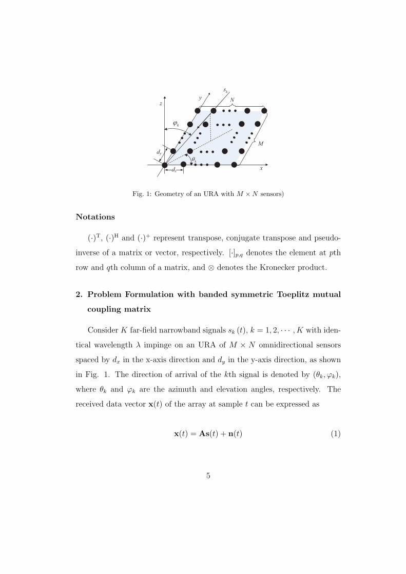
Fig. 1: Geometry of an URA with M ×N sensors)
Notations
(·)T, (·)H and (·)+ represent transpose, conjugate transpose and pseudo-
inverse of a matrix or vector, respectively. [·]p,q denotes the element at pth
row and qth column of a matrix, and ⊗ denotes the Kronecker product.
2. Problem Formulation with banded symmetric Toeplitz mutual
coupling matrix
Consider K far-field narrowband signals sk (t), k = 1, 2, · · · , K with iden-
tical wavelength λ impinge on an URA of M × N omnidirectional sensors
spaced by dx in the x-axis direction and dy in the y-axis direction, as shown
in Fig. 1. The direction of arrival of the kth signal is denoted by (θk, ϕk),
where θk and ϕk are the azimuth and elevation angles, respectively. The
received data vector x(t) of the array at sample t can be expressed as
x(t) = As(t) + n(t) (1)
5
where x(t) = [x1(t), · · · , xN(t), xN+1(t), · · · , x2N(t), · · · , xMN(t)]T holding
the MN received array signals, A = [a(θ1, ϕ1), a(θ2, ϕ2), · · · , a(θK , ϕK)]T is
the array manifold matrix, s(t) = [s1(t), s2(t), · · · , sK(t)]T is the source signal
vector and n(t) = [n1(t), · · · , nN(t), nN+1(t), · · · , n2N(t), · · · , nMN(t)]T is the
additive white Gaussian noise vector. The steering vector a (θk, ϕk) can be
modeled as
a (θk, ϕk) = ay (θk, ϕk)⊗ ax (θk, ϕk) (2)
where
ay (θk, ϕk) = [1, βy (θk, ϕk) , · · · βyM−1 (θk, ϕk)]
T (3)
ax (θk, ϕk) = [1, βx (θk, ϕk) , · · · βxN−1 (θk, ϕk)]
T (4)
with
βy (θk, ϕk) = exp{j2πλ−1dy sin (θk) sin (ϕk)} (5)
βx (θk, ϕk) = exp{j2πλ−1dx cos (θk) sin (ϕk)} (6)
For simplified notation, the pair of angles (θ, ϕ) is omitted in the following
when not causing any confusion.
Considering the effect of mutual coupling, (1) should be modified as
x(t) = CAs(t) + n(t) (7)
where C denotes the mutual coupling matrix (MCM). As indicated in [16, 20,
22], the coupling between neighboring sensors with the same inter-element
spacing is almost the same, while the magnitude of mutual coupling coef-
ficients between two far apart elements would be so small that this effect
can be ignored. Therefore, the mutual coupling of ULA can be modeled
as a banded symmetric Toeplitz matrix. In [20], this model was extended
6
x
y
2
n
1
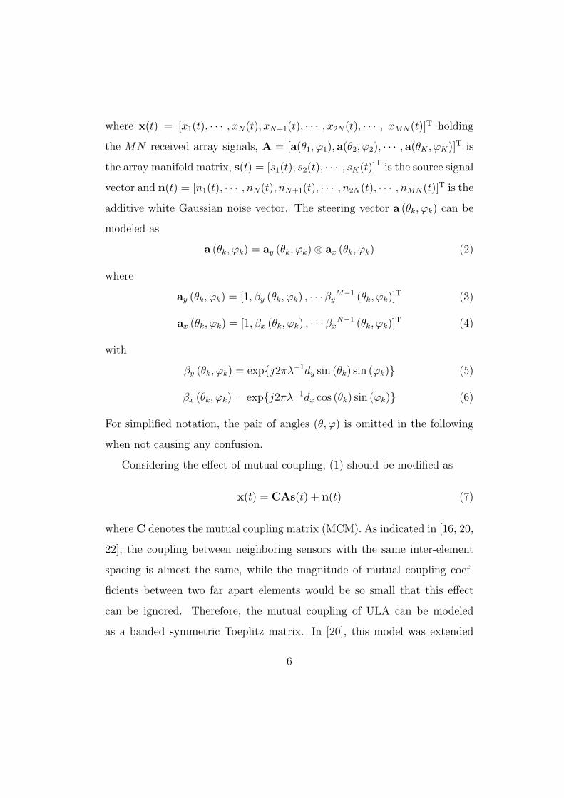
Fig. 2: The mutual coupling model for URAs with P = n+ 1.
to URAs assuming that each sensor is only affected by the 8 immediately
surrounding sensors, and no general mutual coupling model is given. In this
section, we will build a general mutual coupling model for URAs. First, we
define a parameter P as mutual coupling length for URA, which means for
each sensor, we only consider the mutual coupling effect caused by sensors
on the 1st, 2nd, · · · , (P -1)th rectangular grid around it. This definition is
illustrated in Fig. 2 with P = n+ 1. Then the MCM can be expressed as a
block matrix
C =
C1 C2 · · · CP
C2 C1 C2. . .
.... . . . . . . . . . . .
CP C2 C1 C2 CP
. . . . . . . . . . . ....
. . . C2 C1 C2
CP · · · C2 C1
(8)
7
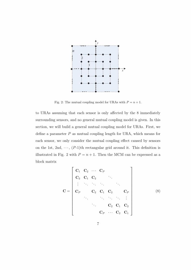
where C is an MN × MN matrix and Ci(i = 1, 2, · · · , P ) are N × N sub-
matrices, where
Ci =
ci−1,0 ci−1,1 · · · ci−1,P−1
ci−1,1 ci−1,0 ci−1,1. . .
... ci−1,1 ci−1,0. . . ci−1,P−1
ci−1,P−1. . . . . . ci−1,1
.... . . ci−1,1 ci−1,0 ci−1,1
ci−1,P−1 · · · ci−1,1 ci−1,0
(9)
The coefficients ci,j denotes the mutual coupling from the sensor located
at (±i,±j), i = 0, j = 0, where (±i,±j) denotes the coordinate of the sensor
in Fig. 2. Especially, we define c0,0 = 1.
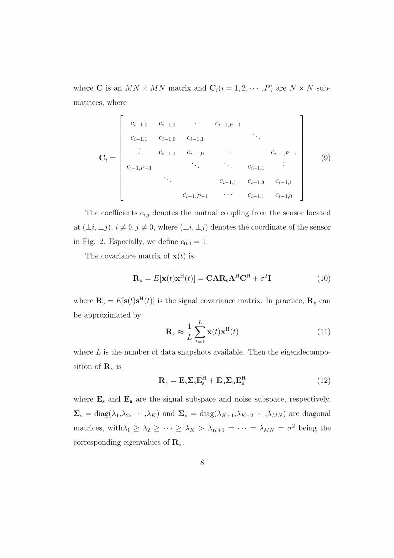
The covariance matrix of x(t) is
Rx = E[x(t)xH(t)] = CARsAHCH + σ2I (10)
where Rs = E[s(t)sH(t)] is the signal covariance matrix. In practice, Rx can
be approximated by
Rx ≈1
L
L∑
t=1
x(t)xH(t) (11)
where L is the number of data snapshots available. Then the eigendecompo-
sition of Rx is
Rx = EsΣsEHs + EnΣnE
Hn (12)
where Es and En are the signal subspace and noise subspace, respectively.
Σs = diag(λ1,λ2, · · · ,λK) and Σn = diag(λK+1,λK+2 · · · ,λMN) are diagonal
matrices, withλ1 ≥ λ2 ≥ · · · ≥ λK > λK+1 = · · · = λMN = σ2 being the
corresponding eigenvalues of Rx.
8
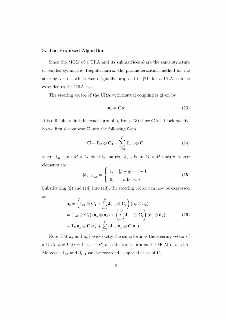
3. The Proposed Algorithm
Since the MCM of a URA and its submatrices share the same structure
of banded symmetric Toeplitz matrix, the parameterization method for the
steering vector, which was originally proposed in [21] for a ULA, can be
extended to the URA case.
The steering vector of the URA with mutual coupling is given by
ac = Ca (13)
It is difficult to find the exact form of ac from (13) since C is a block matrix.
So we first decompose C into the following form
C = IM ⊗C1 +P∑
i=2
Ji−1 ⊗Ci (14)
where IM is an M × M identity matrix. Ji−1 is an M × M matrix, whose
elements are
[Ji−1]p,q =
1, |p− q| = i− 1
0, otherwise(15)
Substituting (2) and (14) into (13), the steering vector can now be expressed
as
ac =
(
IM ⊗C1 +P∑
i=2
Ji−1 ⊗Ci
)
(ay ⊗ ax)
= (IM ⊗C1) (ay ⊗ ax) +
(P∑
i=2
Ji−1 ⊗Ci
)
(ay ⊗ ax)
= IMay ⊗C1ax +P∑
i=2
(Ji−1ay ⊗Ciax)
(16)
Note that ax and ay have exactly the same form as the steering vector of
a ULA, and Ci(i = 1, 2, · · · , P ) also the same form as the MCM of a ULA.
Moreover, IM and Ji−1 can be regarded as special cases of Ci.
9
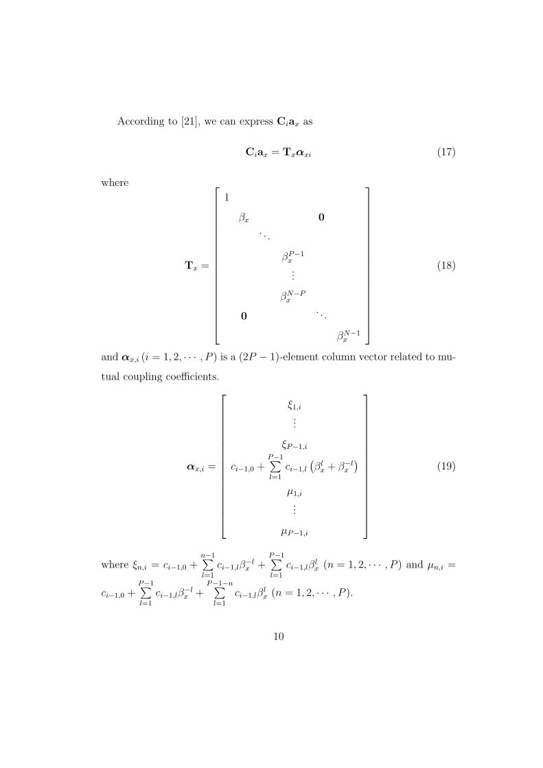
According to [21], we can express Ciax as
Ciax = Txαxi (17)
where
Tx =
1
βx 0
. . .
βP−1x
...
βN−Px
0. . .
βN−1x
(18)
and αx,i (i = 1, 2, · · · , P ) is a (2P − 1)-element column vector related to mu-
tual coupling coefficients.
αx,i =
ξ1,i...
ξP−1,i
ci−1,0 +P−1∑
l=1
ci−1,l
(βlx + β−l
x
)
µ1,i
...
µP−1,i
(19)
where ξn,i = ci−1,0 +n−1∑
l=1
ci−1,lβ−lx +
P−1∑
l=1
ci−1,lβlx (n = 1, 2, · · · , P ) and µn,i =
ci−1,0 +P−1∑
l=1
ci−1,lβ−lx +
P−1−n∑
l=1
ci−1,lβlx (n = 1, 2, · · · , P ).
10
Define ηn as an n-element column vector of ones
ηn =
1, 1, · · · , 1, 1︸ ︷︷ ︸
n
T
(20)
When i = 1
αx,1 = η2P−1 + F′c′0 (21)
where
[F′]p,q =
β−qx + βq
x, q + 1 ≤ p ≤ 2P − q − 1
βqx, p < q + 1
β−qx , p > 2P − q − 1
(22)
c′0 = [c0,1, c0,2, · · · , c0,P−1]T (23)
When i > 1
αx,i = Fci−1 (24)
where
F = [η2P−1,F′] (25)
ci−1 = [ci−1,0, ci−1,1, · · · , ci−1,P−1]T (26)
Similar to (17), we also have
IMay = Tyαy1 (27)
Ji−1ay = Tyαyi (28)
11
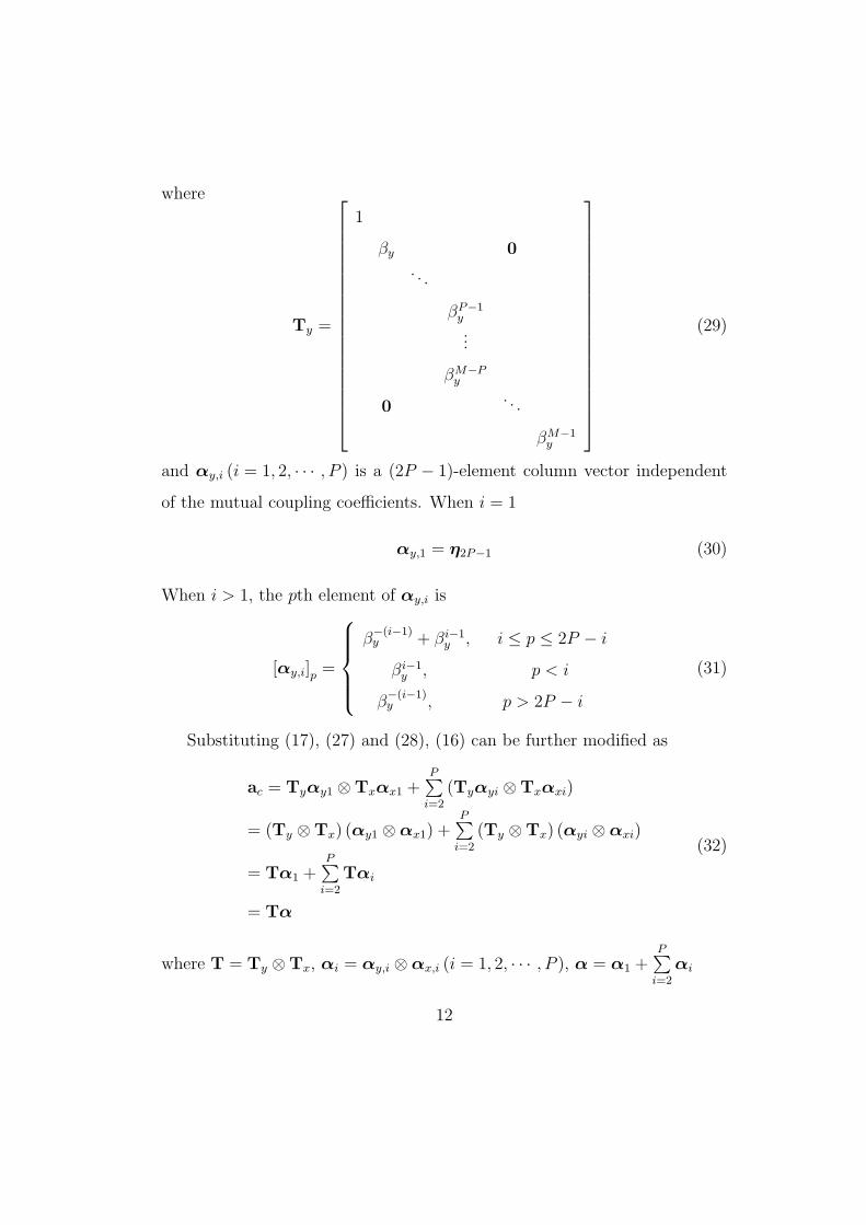
where
Ty =
1
βy 0
. . .
βP−1y
...
βM−Py
0. . .
βM−1y
(29)
and αy,i (i = 1, 2, · · · , P ) is a (2P − 1)-element column vector independent
of the mutual coupling coefficients. When i = 1
αy,1 = η2P−1 (30)
When i > 1, the pth element of αy,i is
[αy,i]p =
β−(i−1)y + βi−1
y , i ≤ p ≤ 2P − i
βi−1y , p < i
β−(i−1)y , p > 2P − i
(31)
Substituting (17), (27) and (28), (16) can be further modified as
ac = Tyαy1 ⊗Txαx1 +P∑
i=2
(Tyαyi ⊗Txαxi)
= (Ty ⊗Tx) (αy1 ⊗αx1) +P∑
i=2
(Ty ⊗Tx) (αyi ⊗αxi)
= Tα1 +P∑
i=2
Tαi
= Tα
(32)
where T = Ty ⊗Tx, αi = αy,i ⊗αx,i (i = 1, 2, · · · , P ), α = α1 +P∑
i=2
αi
12
Now we can see that the steering vector of a URA in the presence of
mutual coupling has a similar form as that of a ULA, which indicates that the
DOA estimation methods developed in [21] based on ULAs can be extended
to the URA case. In the next subsections we will show how to perform this
extension and also use the estimated DOA information to obtain the mutual
coupling coefficients.
3.1. DOA estimation
According to the subspace principle, the noise subspace is orthogonal to
the steering vectors, i.e.
aHc EnE
Hn ac = 0. (33)
From (32), we have derived the result ac = Tα. Then substituting it into
(33), we can obtain the following result directly
αHTHEnEHnTα = 0. (34)
Now define a (2P − 1)2 × (2P − 1)2 matrix M (θ, ϕ)
M (θ, ϕ)∆= THEnE
HnT (35)
Note that if
(2P − 1)2 ≤ MN −K (36)
then, in general, M (θ, ϕ) is of full rank because in this case, the column rank
of En is not less than (2P − 1)2. Therefore, (34) holds true only if M (θ, ϕ)
drops rank so that
rank{M (θ, ϕ)} < (2P − 1)2 (37)
Since the covariance matrix of x(t) is obtained from a finite number of sam-
ples, the reduction of the rank of M (θ, ϕ) can roughly be replaced by the
13
minimum of the determinant of M (θ, ϕ), which indicates that (θ, ϕ) coin-
cides with one of the signal’s DOAs, i.e., (θ, ϕ) = (θk, ϕk) , k = 1, 2, · · · , K.
Therefore, the DOA estimation results can be found from the K highest
peaks of the following function
P (θ, ϕ) =1
det {M (θ, ϕ)}, (38)
where det {·} denotes the determinant of a matrix.
3.2. Mutual coupling coefficients estimation
With the estimated DOA information from (38), we can then proceed to
estimate the mutual coupling coefficients. Using the kth pair of estimated
DOAs, i.e.,(
θk, ϕk
)
, we have
EH
nT(θk, ϕk)α(θk, ϕk) = 0. (39)
From (21), (24), (30), α can be expressed as
α = η(2P−1)2 + η2P−1 ⊗ F′c′0 +P∑
i=2
αy,i ⊗ Fci−1 (40)
or
α = η(2P−1)2 +Gc (41)
where
G = [η2P−1 ⊗ F′, [αy,2, · · · ,αy,P ]⊗ F] (42)
c = [c′0, c1, · · · , cP−1]T
(43)
Substituting (41) into (39)
EHnT
(
η(2P−1)2 +Gc)
= 0 (44)
14
Define F∆= EH
nTG, Z∆= −EH
nTη(2P−1)2 and construct two matrices F∆=
[FT1 ,F
T2 , · · ·F
TK ]
T and Z∆= [ZT
1 ,ZT2 , · · ·Z
TK ]
T, where Fk and Zk denote the F
and Z obtained using the kth pair of estimated DOAs. Then the unknown
mutual coupling coefficients can be obtained by
c = F+Z. (45)
Now the paired angle parameter(
θk, ϕk
)
as well as the mutual coupling
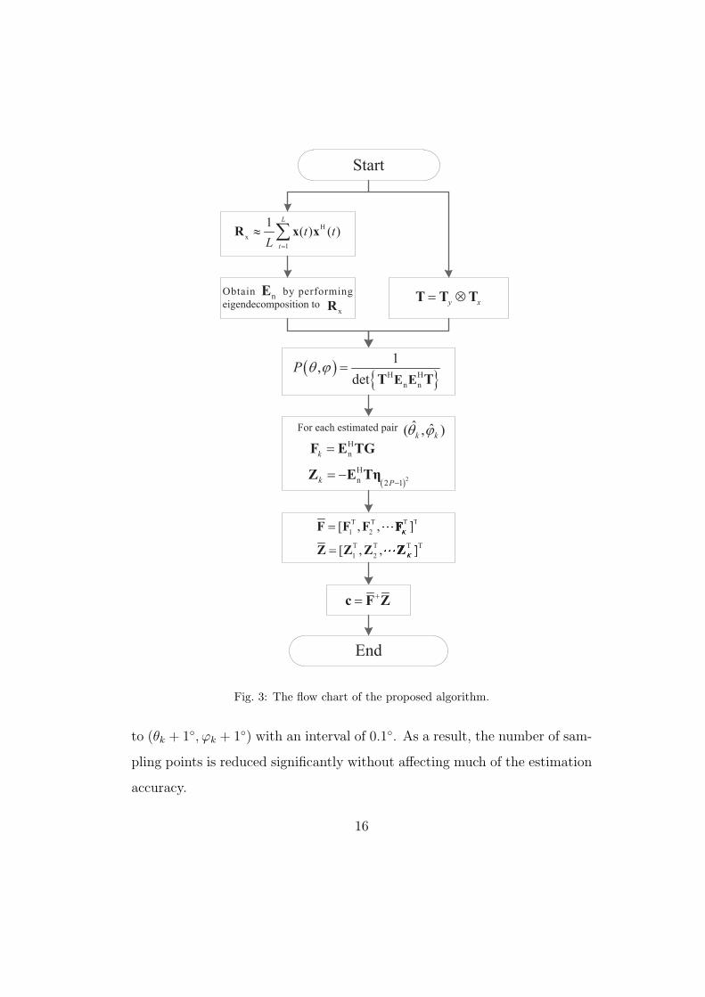
coefficients have been estimated. The proposed algorithm mentioned above
is summarized with the flow chart shown in Fig. 3.
3.3. Computational complexity analysis
To estimate the sample covariance matrix, a computational complex-
ity of O((MN)2L
)is needed. The eigendecomposition operation has a
computational complexity of O((MN)3
). For 2-D spectral searching, at
each DOA sampling point, the matrix T, M, and det{M} should be calcu-
lated, which are associated with a complexity of O (MN), O(MN(MN −
K)(2P − 1)2+(MN − K)(2P − 1)4), and O((MN)3
), respectively. There-
fore, the complexity for the whole 2-D spectral searching process isO(n(MN+
MN(MN−K)(2P − 1)2+(MN−K)(2P − 1)4+(MN)3)), where n =(360◦
∆
)2
is the number of sampling points, with ∆ being the scanning interval, which
is also the accuracy of estimated angles. As an example, for ∆ = 0.1◦,
we have n = 36002. To reduce the computational complexity, we have
adopted the two-level searching method in [20] in our simulations. In the
first round of searching, we find each pair of angles (θk, ϕk) with an interval
of ∆ = 1◦. In the second round, we search in the range of (θk − 1◦, ϕk − 1◦)
15
H
x
1
1( ) ( )
L
t
t tL =
» åR x x
y x= ÄT T T
( ){ }H H
n n
1,
detP q j =
E ET T
Obtain by performing
eigendecomposition tonE
xR
Start
For each estimated pair
H
nk =F E TG
( )2
H
n 2 1k P-= -Z E Tη
� �( , )k kq j
T T T T
1 2[ , , ]
K=F F F F
T T T, ]
T T TT T
K, ], ], ],,,,, ]
T TT, ]
T T T T
1 2[ , , ]
K=Z Z Z Z
T T T, ]
T TT
K]],,,,,,
T TT
+=c F Z
End
Fig. 3: The flow chart of the proposed algorithm.
to (θk + 1◦, ϕk + 1◦) with an interval of 0.1◦. As a result, the number of sam-
pling points is reduced significantly without affecting much of the estimation
accuracy.
16
Now we analyze the complexity for mutual coupling estimation. To
obtain F and Z, the total computational complexity is O(K(MN(MN −
K)(2P − 1)2+(MN−K)(2P − 1)3)). The pseudo inverse of F costsO(K3(MN −K)3).
It needs O(K(MN−K)(2P−1)) to calculate the coefficients in the last step.
4. Simulation Results
In this section, simulation results are provided to demonstrate the perfor-
mance of the proposed algorithm. For all simulations, 4 uncorrelated signals
with the same frequency and power of σ2s from the directions (θ1 = 28◦, ϕ1 = 41◦),
(θ2 = 40◦, ϕ2 = 20◦), (θ3 = 54◦, ϕ3 = 66◦) and (θ4 = 74◦, ϕ4 = 35◦) are con-
sidered. The URA has M = 10 rows and N = 10 columns. Both dx and dy
are half wavelength. The power of additive white Gaussian noise is σ2n and
the signal-to-noise ratio (SNR) is defined as SNR = 10log10(σ2s/σ
2n). We use
root mean square error (RMSE) to evaluate the effectiveness of our algorithm
and 100 Monte Carlo simulations are performed to obain the averaged result.
The RMSE of estimated angles is defined as
RMSE =
√√√√ 1
NmcK
Nmc∑
i=1
K∑
k=1
∣∣∣
(
θik, ϕik
)
− (θk, ϕk)∣∣∣
2
(46)
where Nmc denotes the number of Monte Carlo simulations, and(
θik, ϕik
)
is the estimated (θk, ϕk) in the ith Monte Carlo simulation. The RMSE of
estimated coefficients is defined as
RMSE =
√√√√ 1
Nmc ∥c∥22
Nmc∑
i=1
∥ci − c∥22 (47)
where c is defined in (43), and ci is the estimated c in the ith Monte Carlo
simulation. ∥·∥2 denotes the Euclidean norm.
17
−5 0 5 10 1510
−2
10−1
100
SNR(dB)
RM
SE
(deg
ree)
2D MUSIC, unknown coupling2D MUSIC, known couplingalgorithm in [20]proposed algorithmCRB
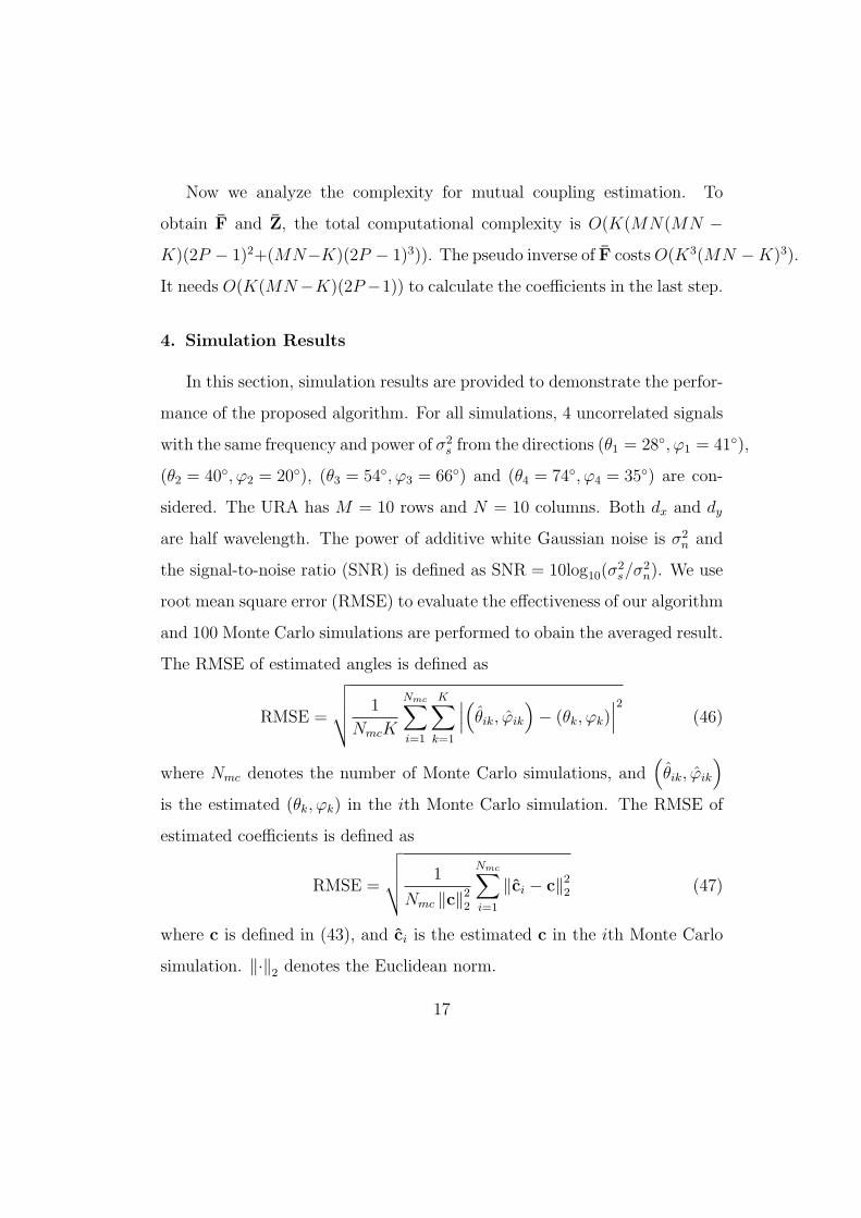
Fig. 4: RMSE of estimated angles versus SNR.
In the first three sets of simulations, we set P = 2, i.e. there are 3
mutual coupling coefficients to estimate and the following values are used
c0,1 = c1,0 = 0.3527 + 0.4854j and c1,1 = 0.0927− 0.2853j.
4.1. Performance versus SNR
First, the performance of the proposed algorithm is studied with a varying
SNR from -5dB to 15dB. The number of data samples is 500. The results are
shown in Fig. 4, where for comparison, those obtained by the algorithm in
[20], 2-D MUSIC with unknown mutual coupling, 2-D MUSIC with known
mutual coupling, and CRB (Cramer-Rao bound) in [20] are also provided.
It can be seen that the 2-D MUSIC with known mutual coupling provides
the best result, while our proposed algorithm has reached a better result
than the one in [20]. As expected, the 2-D MUSIC with unknown mutual
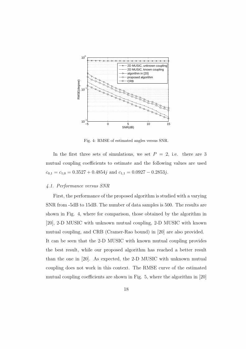
coupling does not work in this context. The RMSE curve of the estimated
mutual coupling coefficients are shown in Fig. 5, where the algorithm in [20]
18
−5 0 5 10 1510
−3
10−2
10−1
100
SNR(dB)
RM
SE
algorithm in [20]proposed algorithmCRB
Fig. 5: RMSE of estimated mutual coupling coefficients versus SNR.
and our proposed one have an almost identical performance and both have
worked effectively.
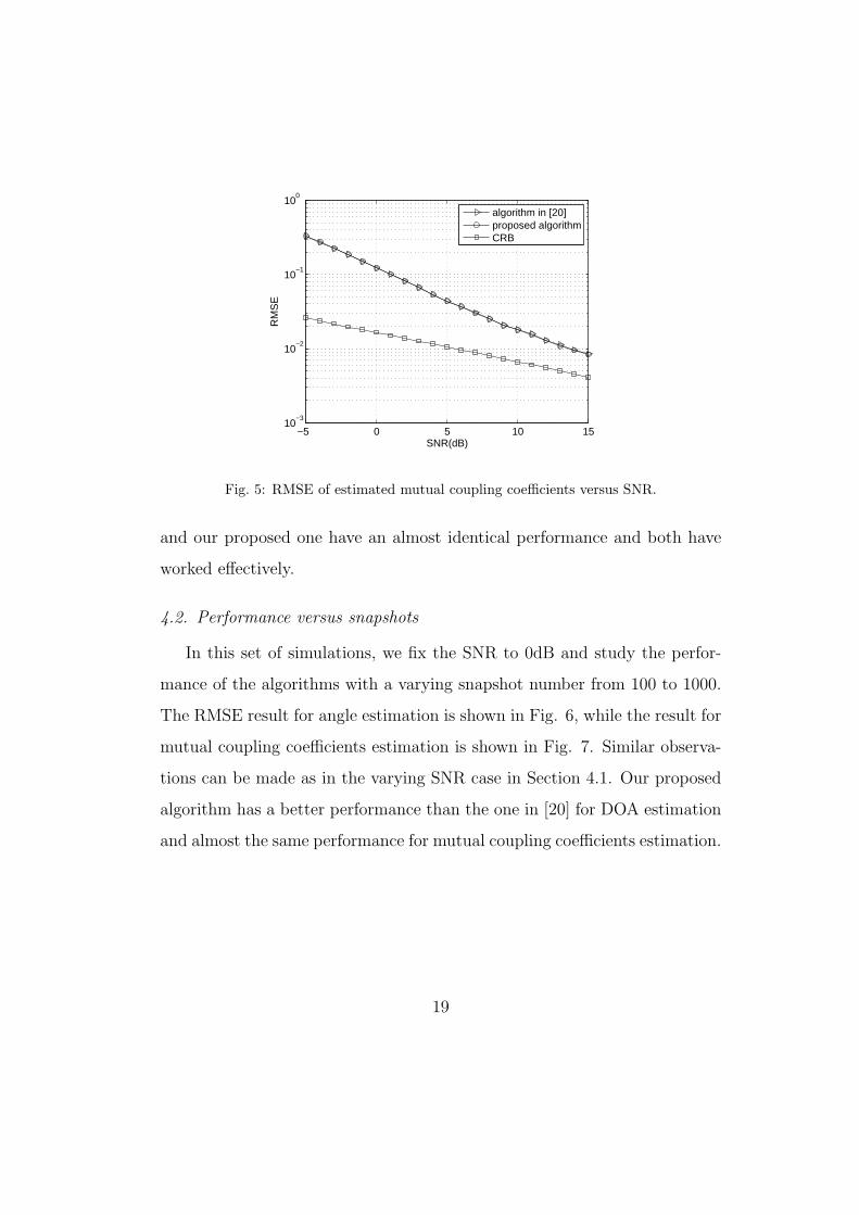
4.2. Performance versus snapshots
In this set of simulations, we fix the SNR to 0dB and study the perfor-
mance of the algorithms with a varying snapshot number from 100 to 1000.
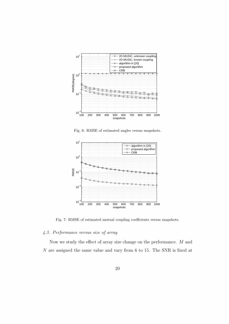
The RMSE result for angle estimation is shown in Fig. 6, while the result for
mutual coupling coefficients estimation is shown in Fig. 7. Similar observa-
tions can be made as in the varying SNR case in Section 4.1. Our proposed
algorithm has a better performance than the one in [20] for DOA estimation
and almost the same performance for mutual coupling coefficients estimation.
19
100 200 300 400 500 600 700 800 900 100010
−2
10−1
100
101
snapshots
RM
SE
(deg
ree)
2D MUSIC, unknown coupling2D MUSIC, known couplingalgorithm in [20]proposed algorithmCRB
Fig. 6: RMSE of estimated angles versus snapshots.
100 200 300 400 500 600 700 800 900 100010
−3
10−2
10−1
100
101
snapshots
RM
SE
algorithm in [20]proposed algorithmCRB
Fig. 7: RMSE of estimated mutual coupling coefficients versus snapshots.
4.3. Performance versus size of array
Now we study the effect of array size change on the performance. M and
N are assigned the same value and vary from 6 to 15. The SNR is fixed at
20
6 7 8 9 10 11 12 13 14 150
0.1
0.2
0.3
0.4
0.5
0.6
0.7
0.8
number of rows(columns)
RM
SE
(deg
ree)
algorithm in [20]proposed algorithmCRB
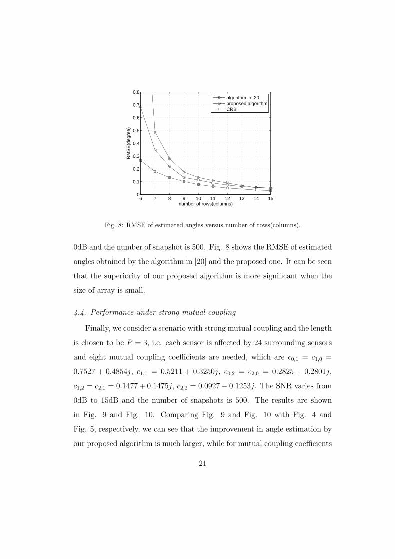
Fig. 8: RMSE of estimated angles versus number of rows(columns).
0dB and the number of snapshot is 500. Fig. 8 shows the RMSE of estimated
angles obtained by the algorithm in [20] and the proposed one. It can be seen
that the superiority of our proposed algorithm is more significant when the
size of array is small.
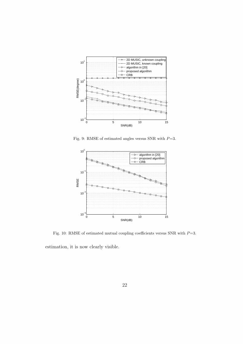
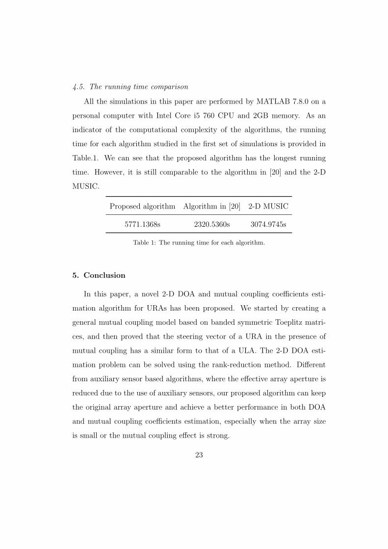
4.4. Performance under strong mutual coupling
Finally, we consider a scenario with strong mutual coupling and the length
is chosen to be P = 3, i.e. each sensor is affected by 24 surrounding sensors
and eight mutual coupling coefficients are needed, which are c0,1 = c1,0 =
0.7527 + 0.4854j, c1,1 = 0.5211 + 0.3250j, c0,2 = c2,0 = 0.2825 + 0.2801j,
c1,2 = c2,1 = 0.1477 + 0.1475j, c2,2 = 0.0927− 0.1253j. The SNR varies from
0dB to 15dB and the number of snapshots is 500. The results are shown
in Fig. 9 and Fig. 10. Comparing Fig. 9 and Fig. 10 with Fig. 4 and
Fig. 5, respectively, we can see that the improvement in angle estimation by
our proposed algorithm is much larger, while for mutual coupling coefficients
21
0 5 10 1510
−2
10−1
100
101
SNR(dB)
RM
SE
(deg
ree)
2D MUSIC, unknown coupling2D MUSIC, known couplingalgorithm in [20]proposed algorithmCRB
Fig. 9: RMSE of estimated angles versus SNR with P=3.
0 5 10 1510
−3
10−2
10−1
100
SNR(dB)
RM
SE
algorithm in [20]proposed algorithmCRB
Fig. 10: RMSE of estimated mutual coupling coefficients versus SNR with P=3.
estimation, it is now clearly visible.
22
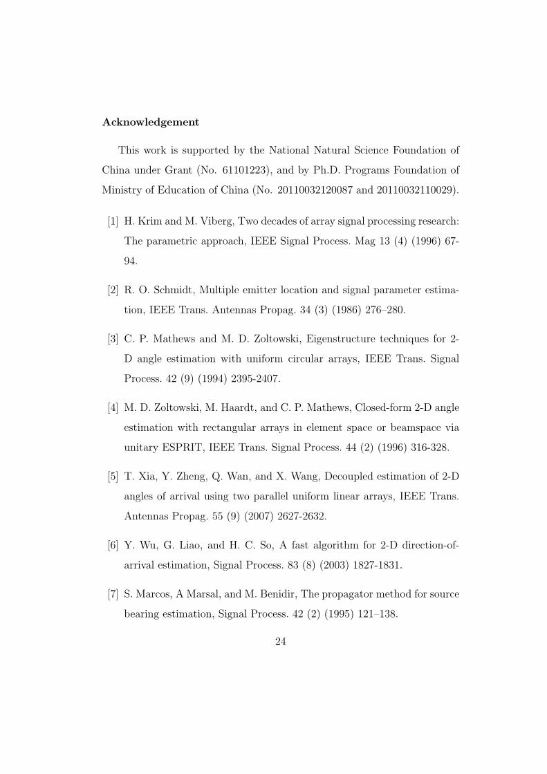
4.5. The running time comparison
All the simulations in this paper are performed by MATLAB 7.8.0 on a
personal computer with Intel Core i5 760 CPU and 2GB memory. As an
indicator of the computational complexity of the algorithms, the running
time for each algorithm studied in the first set of simulations is provided in
Table.1. We can see that the proposed algorithm has the longest running
time. However, it is still comparable to the algorithm in [20] and the 2-D
MUSIC.
Proposed algorithm Algorithm in [20] 2-D MUSIC
5771.1368s 2320.5360s 3074.9745s
Table 1: The running time for each algorithm.
5. Conclusion
In this paper, a novel 2-D DOA and mutual coupling coefficients esti-
mation algorithm for URAs has been proposed. We started by creating a
general mutual coupling model based on banded symmetric Toeplitz matri-
ces, and then proved that the steering vector of a URA in the presence of
mutual coupling has a similar form to that of a ULA. The 2-D DOA esti-
mation problem can be solved using the rank-reduction method. Different
from auxiliary sensor based algorithms, where the effective array aperture is
reduced due to the use of auxiliary sensors, our proposed algorithm can keep
the original array aperture and achieve a better performance in both DOA
and mutual coupling coefficients estimation, especially when the array size
is small or the mutual coupling effect is strong.
23
Acknowledgement
This work is supported by the National Natural Science Foundation of
China under Grant (No. 61101223), and by Ph.D. Programs Foundation of
Ministry of Education of China (No. 20110032120087 and 20110032110029).
[1] H. Krim and M. Viberg, Two decades of array signal processing research:
The parametric approach, IEEE Signal Process. Mag 13 (4) (1996) 67-
94.
[2] R. O. Schmidt, Multiple emitter location and signal parameter estima-
tion, IEEE Trans. Antennas Propag. 34 (3) (1986) 276–280.
[3] C. P. Mathews and M. D. Zoltowski, Eigenstructure techniques for 2-
D angle estimation with uniform circular arrays, IEEE Trans. Signal
Process. 42 (9) (1994) 2395-2407.
[4] M. D. Zoltowski, M. Haardt, and C. P. Mathews, Closed-form 2-D angle
estimation with rectangular arrays in element space or beamspace via
unitary ESPRIT, IEEE Trans. Signal Process. 44 (2) (1996) 316-328.
[5] T. Xia, Y. Zheng, Q. Wan, and X. Wang, Decoupled estimation of 2-D
angles of arrival using two parallel uniform linear arrays, IEEE Trans.
Antennas Propag. 55 (9) (2007) 2627-2632.
[6] Y. Wu, G. Liao, and H. C. So, A fast algorithm for 2-D direction-of-
arrival estimation, Signal Process. 83 (8) (2003) 1827-1831.
[7] S. Marcos, A Marsal, and M. Benidir, The propagator method for source
bearing estimation, Signal Process. 42 (2) (1995) 121–138.
24
[8] N. Tayem and H. M. Kwon, L-shape 2-dimensional arrival angle esti-
mation with propagator method, IEEE Trans. Antennas Propag. 53 (5)
(2005) 1622-1630.
[9] J. Liang and D. Liu, Joint elevation and azimuth direction finding using
L-shaped array, IEEE Trans. Antennas Propag. 58 (6) (2010) 2136-2141.
[10] X. Nie and L. Li, A Computationally Efficient Subspace Algorithm for
2-D DOA Estimation with L-shaped Array, IEEE Signal Process. Lett.
21 (8) (2014) 971-974.
[11] W. Zhang, W. Liu, J. Wang, and S. Wu, Computationally efficient 2-D
DOA estimation for uniform rectangular arrays, Multidim. Syst. Sign.
Process. 25 (4) (2014) 847-857.
[12] C. Roller and W. Wasylkiwskyj, Effects of mutual coupling on super-
resolution DF in linear arrays, Proc. IEEE Int. Conf. Acoust., Speech
Signal Process. (5) (1992) 257-260.
[13] A. J. Weiss and B. Friedlander, Mutual coupling effects on phase-only
direction finding, IEEE Trans. Antennas Propag. 40 (5) (1992) 535-541.
[14] B. H. Wang, H. T. Hui and M. S. Leong, Decoupled 2D direction of
arrival estimation using compact uniform circular arrays in the presence
of elevation-dependent mutual coupling, IEEE Trans. Antennas Propag.
58 (3) (2010) 747-755.
[15] J. Dai, X. Bao, N. Hu, C. Chang, and W. Xu, A recursive RARE al-
gorithm for DOA estimation with unknown mutual coupling, IEEE An-
tennas Wireless Propag. Lett. 13 (2014) 1593-1596.
25
[16] B. Friedlander, and A. J. Weiss, Direction finding in the presence of
mutual coupling, IEEE Trans. Antennas Propag. 39, (3) (1991) 273–
284.
[17] M. Pesavento, A. B. Gershman, and K. M. Wong, Direction finding in
partly calibrated sensor arrays composed of multiple subarrays, IEEE
Trans. Signal Process. 50 (9) (2002) 2103–2115.
[18] C. Liu, Z. Ye, and Y. Zhang, Autocalibration algorithm for mutual
coupling of planar array, Signal Process. 90 (3) (2010) 784-794.
[19] J. Liang, X. Zeng, W. Wang, and H. Chen, L-shaped array-based eleva-
tion and azimuth direction finding in the presence of mutual coupling,
Signal Process. 91 (50) (2011) 1319-1328.
[20] Z. Ye and C. Liu, 2-D DOA estimation in the presence of mutual cou-
pling, IEEE Trans. Antennas Propag. 56 (10) (2008) 3150-3158.
[21] B. Liao, Z. G. Zhang, and S. C. Chan, DOA estimation and tracking of
ULAs with mutual coupling, IEEE Trans. Aerospace Electronic Systems.
48 (1) (2012) 891–905.
[22] T. Svantesson, Modeling and estimation of mutual coupling in a uniform
linear array of dipoles, in Proc. IEEE Int. Conf. Acoust., Speech Signal
Process. (5) (1999) 2961-2964.
26