Direct Transient Response
24
WORKSHOP 3 Direct Transient Response Analysis MSC.Nastran 102 Exercise Workbook 3-1 Objectives ■ Define time-varying excitation. ■ Produce a MSC.Nastran input file from dynamic math model created in Workshop 1. ■ Submit the file for analysis in MSC.Nastran. ■ Compute nodal displacements for desired time domain.
description
Direct Transient Response
Transcript of Direct Transient Response

WORKSHOP 3
Direct Transient Response Analysis
MSC.Nastran 102 Exercise Workbook 3-1
Objectives
■ Define time-varying excitation.
■ Produce a MSC.Nastran input file from dynamic math model created in Workshop 1.
■ Submit the file for analysis in MSC.Nastran.
■ Compute nodal displacements for desired time domain.

3-2 MSC.Nastran 102 Exercise Workbook
WORKSHOP 3 Direct Transient Response Analysis
MSC.Nastran 102 Exercise Workbook 3-3
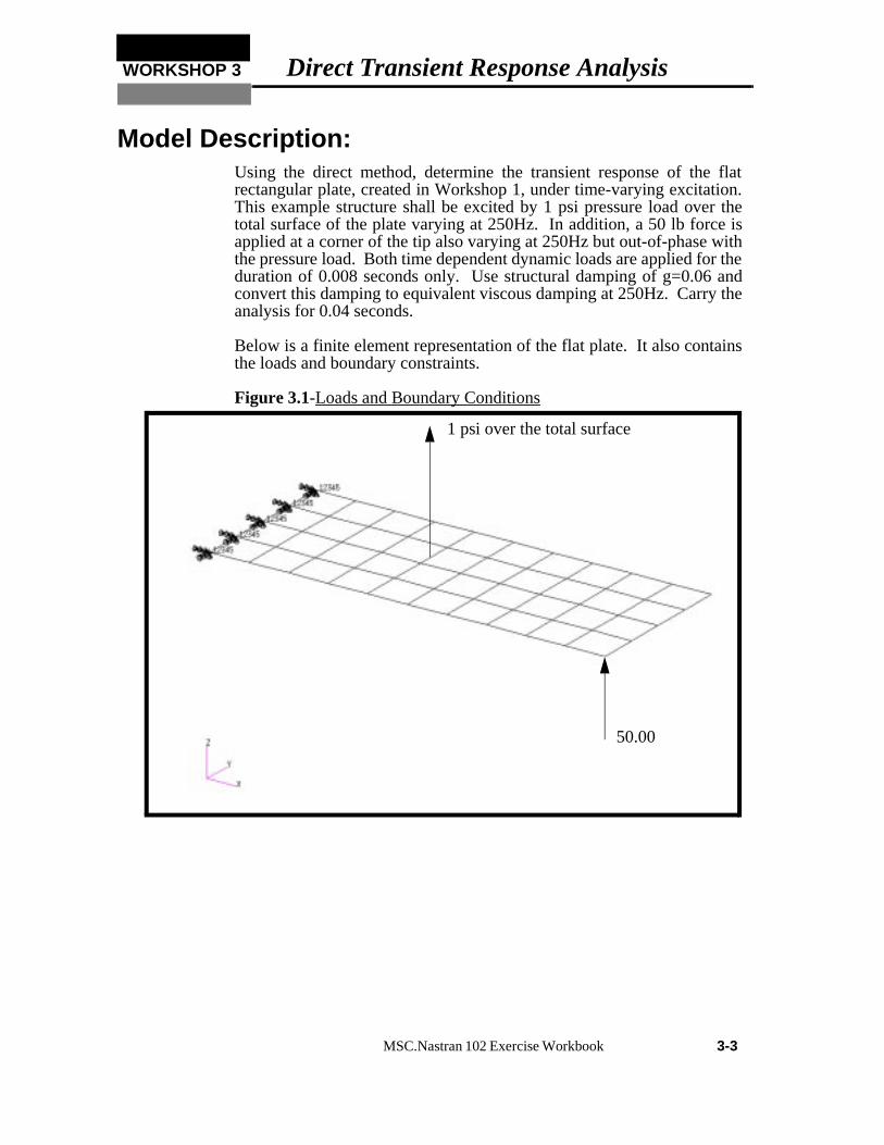
Model Description:Using the direct method, determine the transient response of the flatrectangular plate, created in Workshop 1, under time-varying excitation.This example structure shall be excited by 1 psi pressure load over thetotal surface of the plate varying at 250Hz. In addition, a 50 lb force isapplied at a corner of the tip also varying at 250Hz but out-of-phase withthe pressure load. Both time dependent dynamic loads are applied for theduration of 0.008 seconds only. Use structural damping of g=0.06 andconvert this damping to equivalent viscous damping at 250Hz. Carry theanalysis for 0.04 seconds.
Below is a finite element representation of the flat plate. It also containsthe loads and boundary constraints.
Figure 3.1-Loads and Boundary Conditions
1 psi over the total surface
50.00

3-4 MSC.Nastran 102 Exercise Workbook
Suggested Exercise Steps
■ Reference previously created dynamic math model, plate.bdf, by using the INCLUDE statement.
■ Define the time-varying pressure loading (PLOAD2, LSEQ and TLOAD2). (Hint, be certain to specify phase angle since the applied loads are out-of-phase).
■ Define the time-varying tip load (DAREA and TLOAD2). (Again, be certain to specify the phase angle).
■ Combine the time-varying loads (DLOAD).
■ Specify integration time steps (TSTEP).
■ Prepare the model for a direct transient analysis (SOL 109).
■ Specify the structural damping and convert this damping to equivalent viscous damping.
■ PARAM, G, 0.06
■ PARAM, W3, 1571.0
■ Request response in terms of nodal displacement at grid points 11, 33 and 55.
■ Generate an input file and submit it to the MSC.Nastran solver for direct transient analysis.
■ Review the results, specifically the nodal displacements and xy-plot output.

WORKSHOP 3 Direct Transient Response Analysis
MSC.Nastran 102 Exercise Workbook 3-5
ID SEMINAR,PROB3______________________________________________________________________________________________________________________________________________________________________________________________________________________________________________________________________________________________________________________________________________________________________________________________________________________________________________________________________________CEND________________________________________________________________________________________________________________________________________________________________________________________________________________________________________________________________________________________________________________________________________________________________________________________________________________________________________________________________________________________________________________________________________________________________________________________________________________________________________________________________________________________________________________________________________________________________________________________________________________________________________________________________________________________________________________________________________________________________________________________________________________________________________________________________________________________________________________________________________________________________________________________________________________________________________________________________________________________________________________________________________________________________________________________________________________________________________________________________________________________________________________________________________________________________________________________________________________________________________________________________________________________BEGIN BULK

3-6 MSC.Nastran 102 Exercise Workbook
1 2 3 4 5 6 7 8 9 10

WORKSHOP 3 Direct Transient Response Analysis
MSC.Nastran 102 Exercise Workbook 3-7
1 2 3 4 5 6 7 8 9 10
ENDDATA

3-8 MSC.Nastran 102 Exercise Workbook
Exercise Procedure:1. Users who are not utilizing MSC.Patran for generating an input file
should go to Step 13, otherwise, proceed to step 2.
2. Open a new database named prob3.db.
In the New Model Preferences form, set the following:
3. Create the model by importing an existing MSC.Nastran input file,(plate.bdf).
4. Activate the entity labels by selecting the Show Labels icon on the tool-bar.
File/New
New Database Name prob3
OK
Tolerance ◆ Default
Analysis Code: MSC/NASTRAN
OK
◆ Analysis
Action: Read Input File
Object: Model Data
Method Translate
Select Input File
Select File plate.bdf
OK
Apply
OK
Show Labels

WORKSHOP 3 Direct Transient Response Analysis
MSC.Nastran 102 Exercise Workbook 3-9
5. Add the pre-defined constraints into the default load case.
6. Create a time-dependent field for the transient response of the pressureloading.
◆ Load Cases
Action: Create
Load Case Name transient_response
Load Case Type: Time Dependent
Assign/Prioritize Loads/BCs
Select Individual Load/BCs (Select from menu.)
Displ_spc1.1
OK
Apply
◆ Fields
Action: Create
Object: Non Spatial
Method Tabular Input
Field Name time_dependent_pressure
[Options ...]
Maximum Number of t 21
OK
Input Data ...
Map Function to Table...
PCL Expression f ’(t): sind(360.*250.*’t)
Start Time 0.0
End Time 0.008
Number of Points 20
Apply

3-10 MSC.Nastran 102 Exercise Workbook
In the Time/Frequency Scalar Table Data window, add the following toRow 21:
7. Create another time-dependent field for the transient response of thenodal force.
Cancel
Time(t) Value
21 0.04 0.0
OK
Apply
◆ Fields
Action: Create
Object: Non Spatial
Method Tabular Input
Field Name time_dependent_force
[Options ...]
Maximum Number of t 21
OK
Input Data ...
Map Function to Table...
PCL Expression f ’(t) -sind(360*250*’t)
Start Time 0.0
End Time 0.008
Number of Points 20
Apply
Cancel

WORKSHOP 3 Direct Transient Response Analysis
MSC.Nastran 102 Exercise Workbook 3-11
In the Time/Frequency Scalar Table Data window, add the following toRow 21:
8. Create the time dependent pressure.
Note: The default direction of pressure in MSC.Patran is oppositefrom default MSC.Nastran assumption.
Time(t) Value
21 0.04 0.0
OK
Apply
◆ Loads/BCs
Action: Create
Object: Pressure
Type: Element Uniform
New Set Name pressure
Target Element Type: 2D
Input Data...
Top Surf Pressure -1
* Time/Freq. Dependence:(Select from the Time Dependent Fields box)
f:time_dependent_pressure
OK
Select Application Region...
◆ FEM
Select 2D Elements or Edge(Select all elements)
Elem 1:40
Add
OK
Apply
3-12 MSC.Nastran 102 Exercise Workbook
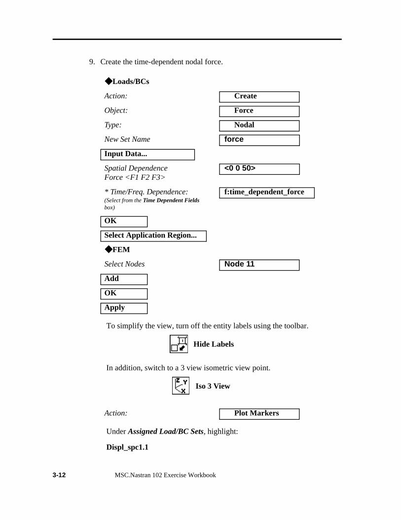
9. Create the time-dependent nodal force.
To simplify the view, turn off the entity labels using the toolbar.
In addition, switch to a 3 view isometric view point.
Under Assigned Load/BC Sets, highlight:
Displ_spc1.1
◆ Loads/BCs
Action: Create
Object: Force
Type: Nodal
New Set Name force
Input Data...
Spatial DependenceForce <F1 F2 F3>
<0 0 50>
* Time/Freq. Dependence:(Select from the Time Dependent Fields box)
f:time_dependent_force
OK
Select Application Region...
◆ FEM
Select Nodes Node 11
Add
OK
Apply
Action: Plot Markers
Hide Labels
Iso 3 View

WORKSHOP 3 Direct Transient Response Analysis
MSC.Nastran 102 Exercise Workbook 3-13
Force_force
Press_pressure
Under Select Groups, highlight:
default_group
The result should be similar to Figure 3.2.
Figure 3.2-The model with loads and boundary conditions applied.
10. Create the analysis.
◆ Analysis
Action: Analyze
Object: Entire Model
Method: Analysis Deck
Job Name prob3
Solution Type...
Translation Parameters...
Data Output: XDB and Print
OK
Solution Type: ◆ TRANSIENT RESPONSE
XY
Z
12345
50.00
12345
12345 12345
12345
1.0001.000
1.0001.000
1.0001.000
1.0001.000
1.0001.000
1.0001.000
1.0001.000
1.0001.000
1.0001.000
1.0001.000
1.0001.000
1.0001.000
1.0001.000
1.0001.000
1.0001.000
1.0001.000
1.0001.000
1.0001.000
1.0001.000
1.0001.000
XY
Z

3-14 MSC.Nastran 102 Exercise Workbook
Under Output Requests, highlight:
SPCFORCES(SORT1,Real)=All FEM
Formulation: Direct
Solution Parameters...
Mass Calculation: Coupled
Wt.-Mass Conversion = .00259
Struct. Damping Coeff. = 0.06
W3, Damping Factor = 1571
OK
OK
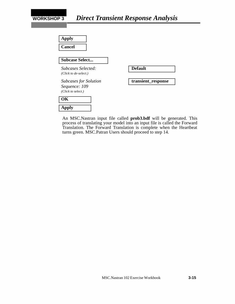
Subcase Create...
Available Subcases(Select from menu.)
transient_response
Subcase Parameters...
Time Recovery Points DEFINE TIME STEPS ...
Number of Time Steps = 100
Delta - T(Hit Return to Input Data.
.0004
OK
OK
Output Requests...
Form Type: Advanced
Delete
Output Requests: select DISPLACEMENT(...
Options/Sorting: By Freq/Time
Modify
OK
WORKSHOP 3 Direct Transient Response Analysis
MSC.Nastran 102 Exercise Workbook 3-15
An MSC.Nastran input file called prob3.bdf will be generated. Thisprocess of translating your model into an input file is called the ForwardTranslation. The Forward Translation is complete when the Heartbeatturns green. MSC.Patran Users should proceed to step 14.
Apply
Cancel
Subcase Select...
Subcases Selected:(Click to de-select.)
Default
Subcases for Solution Sequence: 109(Click to select.)
transient_response
OK
Apply

3-16 MSC.Nastran 102 Exercise Workbook
Generating an input file for MSC.Nastran Users:MSC.Nastran users can generate an input file using the data previouslystated. The result should be similar to the output below.
11. MSC.Nastran input file: prob3.dat
ID SEMINAR, PROB3
SOL 109
TIME 30
CEND
TITLE= TRANSIENT RESPONSE WITH TIME DEPENDENT PRESSURE AND POINT LOADS
SUBTITLE= USE THE DIRECT METHOD
ECHO= PUNCH
SPC= 1
SET 1= 11, 33, 55
DISPLACEMENT= 1
SUBCASE 1
DLOAD= 700 $ SELECT TEMPORAL COMPONENT OF TRANSIENT LOADING
LOADSET= 100 $ SELECT SPACIAL DISTRIBUTION OF TRANSIENT LOADING
TSTEP= 100 $ SELECT INTEGRATION TIME STEPS
$
OUTPUT (XYPLOT)
XGRID=YES
YGRID=YES
XTITLE= TIME (SEC)
YTITLE= DISPLACEMENT RESPONSE AT LOADED CORNER
XYPLOT DISP RESPONSE / 11 (T3)
YTITLE= DISPLACEMENT RESPONSE AT CENTER TIP
XYPLOT DISP RESPONSE / 33 (T3)
YTITLE= DISPLACEMENT RESPONSE AT OPPOSITE CORNER
XYPLOT DISP RESPONSE / 55 (T3)
$
BEGIN BULK
PARAM, COUPMASS, 1
PARAM, WTMASS, 0.00259
$
$ PLATE MODEL DESCRIBED IN NORMAL MODES EXAMPLE
$
INCLUDE ’plate.bdf’
$
$ SPECIFY STRUCTURAL DAMPING
$ 3 PERCENT AT 250 HZ. = 1571 RAD/SEC.
$
PARAM, G, 0.06

WORKSHOP 3 Direct Transient Response Analysis
MSC.Nastran 102 Exercise Workbook 3-17
PARAM, W3, 1571.
$
$ APPLY UNIT PRESSURE LOAD TO PLATE
$
LSEQ, 100, 300, 400
$
PLOAD2, 400, 1., 1, THRU, 40
$
$ VARY PRESSURE LOAD (250 HZ)
$
TLOAD2, 200, 300, , 0, 0., 8.E-3, 250., -90.
$
$ APPLY POINT LOAD OUT OF PHASE WITH PRESSURE LOAD
$
TLOAD2, 500, 600, , 0, 0., 8.E-3, 250., 90.
$
DAREA, 600, 11, 3, 1.
$
$ COMBINE LOADS
$
DLOAD, 700, 1., 1., 200, 50., 500
$
$ SPECIFY INTERGRATION TIME STEPS
$
TSTEP, 100, 100, 4.0E-4, 1
$
ENDDATA

3-18 MSC.Nastran 102 Exercise Workbook
Submitting the input file for analysis:
12. Submit the input file to MSC.Nastran for analysis.
12a. To submit the MSC.Patran .bdf file for analysis, find anavailable UNIX shell window. At the command promptenter: nastran prob3.bdf scr=yes. Monitor the run usingthe UNIX ps command.
12b. To submit the MSC.Nastran .dat file for analysis, find anavailable UNIX shell window. At the command promptenter: nastran prob3 scr=yes. Monitor the run using theUNIX ps command.
13. When the run is completed, use plotps utility to create apostscript file, prob3.ps, from the binary plot file prob3.plt.The displacement response plots for Grids 11, 33 and 55 areshown in figures 3.2, 3.3 and 3.4.
14. Edit the prob3.f06 file and search for the word FATAL. Ifno matches exist, search for the word WARNING.Determine whether existing WARNING messages indicatemodeling errors.
15. While still editing prob3.f06, search for the word:
D I S P L (spaces are necessary)
Displacement at Grid 11
Time T3
.0024 = __________
.0052 = __________
.02 = __________
Displacement at Grid 33
Time T3
.0024 = __________
.0052 = __________
.02 = __________

WORKSHOP 3 Direct Transient Response Analysis
MSC.Nastran 102 Exercise Workbook 3-19
Displacement at Grid 55
Time T3
.0024 = __________
.0052 = __________
.02 = __________

3-20 MSC.Nastran 102 Exercise Workbook
Comparison of Results
16. Compare the results obtained in the .f06 file with the following results:
17. MSC.Nastran Users have finished this exercise. MSC.PatranUsers should proceed to the next step.
POINT-ID = 11
D I S P L A C E M E N T V E C T O R
TIME TYPE T1 T2 T3 R1 R2 R3
0.0 G 0.0 0.0 0.0 0.0 0.0 0.0
4.000000E-04 G 0.0 0.0 -2.173625E-02 1.104167E-02 1.050818E-02 0.0
8.000000E-04 G 0.0 0.0 -7.204904E-02 2.847414E-02 2.852519E-02 0.0
1.200000E-03 G 0.0 0.0 -1.433462E-01 4.082027E-02 4.915178E-02 0.0
.
.
.
3.879996E-02 G 0.0 0.0 -3.726422E-02 -6.629907E-05 1.039267E-02 0.0
3.919996E-02 G 0.0 0.0 -2.122380E-02 -1.431050E-05 5.916678E-03 0.0
3.959996E-02 G 0.0 0.0 -2.998187E-03 -7.089762E-06 8.371174E-04 0.0
3.999996E-02 G 0.0 0.0 1.535974E-02 5.380207E-06 -4.281030E-03 0.0
POINT-ID = 33
D I S P L A C E M E N T V E C T O R
TIME TYPE T1 T2 T3 R1 R2 R3
0.0 G 0.0 0.0 0.0 0.0 0.0 0.0
4.000000E-04 G 0.0 0.0 -1.122398E-02 9.220218E-03 6.138594E-03 0.0
8.000000E-04 G 0.0 0.0 -4.424753E-02 2.576699E-02 2.014980E-02 0.0
1.200000E-03 G 0.0 0.0 -1.030773E-01 3.819036E-02 3.922388E-02 0.0
.
.
.
3.879996E-02 G 0.0 0.0 -3.729695E-02 1.898676E-05 1.037927E-02 0.0
3.919996E-02 G 0.0 0.0 -2.121863E-02 3.488550E-05 5.907703E-03 0.0
3.959996E-02 G 0.0 0.0 -3.002583E-03 -2.228106E-07 8.361273E-04 0.0
3.999996E-02 G 0.0 0.0 1.535096E-02 -3.032754E-05 -4.274252E-03 0.0
POINT-ID = 55
D I S P L A C E M E N T V E C T O R
TIME TYPE T1 T2 T3 R1 R2 R3
0.0 G 0.0 0.0 0.0 0.0 0.0 0.0
4.000000E-04 G 0.0 0.0 -2.849185E-03 7.791447E-03 4.611430E-03 0.0
8.000000E-04 G 0.0 0.0 -1.992890E-02 2.322436E-02 1.681028E-02 0.0
1.200000E-03 G 0.0 0.0 -6.643156E-02 3.540079E-02 3.501805E-02 0.0
.
.
.
3.879996E-02 G 0.0 0.0 -3.722652E-02 1.035188E-04 1.039059E-02 0.0
3.919996E-02 G 0.0 0.0 -2.115454E-02 8.268487E-05 5.912832E-03 0.0
3.959996E-02 G 0.0 0.0 -2.998628E-03 6.654292E-06 8.371378E-04 0.0
3.999996E-02 G 0.0 0.0 1.529953E-02 -6.482315E-05 -4.277684E-03 0.0

WORKSHOP 3 Direct Transient Response Analysis
MSC.Nastran 102 Exercise Workbook 3-21
18. Proceed with the Reverse Translation process, that is attachingthe prob3.xdb results file into MSC.Patran. To do this, returnto the Analysis form and proceed as follows:
When the translation is complete bring up the Results form.
◆ Analysis
Action: Attach XDB
Object: Result Entities
Method Local
Select Results File...
Select File prob3.xdb
OK
Apply
◆ Results
Action: Create
Object: Graph
Select Results Cases Transient_response, 0 of 101 subcases
Filter Method All
Filter
Apply
Close
y: Result
Select y Result: Displacement, Translational
Quanity: Z Component
x: Global Variable
Variable: Time
Select the target entities form by clicking on this Icon
Target Entities

3-22 MSC.Nastran 102 Exercise Workbook
You may reset the graphics by clicking on this icon :
Figure 3.3-Displacement Response at Node 11
To Plot Node 33 and 55, simply select them..
Target Entities
Select Nodes: Node 11
Apply
Select Nodes: Node 33
Apply
Reset Graphics

WORKSHOP 3 Direct Transient Response Analysis
MSC.Nastran 102 Exercise Workbook 3-23
Figure 3.4-Displacement Response at Node 33
Figure 3.5-Displacement Response at Node 55
Quit MSC.Patran when you are finished with this exercise.
Select Nodes: Node 55
Apply

3-24 MSC.Nastran 102 Exercise Workbook