
Direct Simulation Monte Carlo Method for Cold Atom ...
107
Direct Simulation Monte Carlo Method for Cold Atom Dynamics: Boltzmann Equation in the Quantum Collision Regime Andrew Christopher James Wade a thesis submitted for the degree of Master of Science at the University of Otago, Dunedin, New Zealand. July 27, 2012
Transcript of Direct Simulation Monte Carlo Method for Cold Atom ...

Direct Simulation Monte Carlo
Method for Cold Atom
Dynamics: Boltzmann Equation
in the Quantum Collision Regime
Andrew Christopher James Wade
a thesis submitted for the degree of
Master of Science
at the University of Otago, Dunedin,
New Zealand.
July 27, 2012

Abstract
In this thesis we develop a direct simulation Monte Carlo (DSMC) method for
simulating highly nonequilibrium dynamics of nondegenerate ultra cold gases.
We show that our method can simulate the high-energy collision of two thermal
clouds in the regime observed in experiments [Thomas et al. Phys. Rev. Lett. 93,
173201 (2004)], which requires the inclusion of beyond s-wave scattering. We
also consider the long-time dynamics of this system, demonstrating that this
would be a practical experimental scenario for testing the Boltzmann equation
and studying rethermalization. A quantum DSMC algorithm is also discussed.
iii


Acknowledgements
There are many whom I wish to thank for the opportunities they have given me,
be it directly, or for the unconscious support of a friend. Here are a few...
First of all my supervisor and friend Assoc. Prof. Blair Blakie for the freedom,
accessibility, insight and morale boosts in those painful Masters moments. For
the privileges of conferences, summer courses, group meetings, and finally, for
the general academic advice and continuing support.
My collaborators and substitute supervisors when Blair had had enough and left
the country periodically: Danny Baillie, Dr. Ashton Bradley, Dr. Niels Kjaer-
gaard, and Dr. Eite Tiesinga. Danny for being my coding guru and his intense
critiquing, such as noting "should be good/sweet as" is not the best scientific
terminology for an article. Ashton for entertaining many of my "fruitful" dis-
cussions. Niels for his physics and fishing advice.
My friends for the good times, and my colleagues whom share the same pains.
My family, who are always with me.
Finally, my beloved Line.
v


Abbreviations and Notation
Here, we give tables of the notation and the abbreviations used in this thesis. We do notinclude commonly used notation, e.g., r as the position vector or T as temperature, andnotation that is not used in more than one section. The reference gives the page in whichthey are first introduced.
Table 1: Abbreviations.Abbreviation Description ReferenceBE Boltzmann equation. 1ZNG Zaremba-Nikuni-Griffin. 1DSMC Direct simulation Monte Carlo. 2LATS Locally adaptive time step. 3LAC Locally adaptive cell. 3Kn Knudsen number. 13NNC Nearest neighbor collision. 15TASC Transient adaptive subcell. 21LSD Locally sampled density. 79FFT Fast Fourier Transform. 85
Table 2: Notation.Notation Description ReferenceTcoll Collision energy. 2vr Magnitude of the relative velocity. 2f ≡ f (p, r, t) Semiclassically phase-space distribution function. 7n (r, t) Position space density. 7U (r, t) Potential. 7asc s-wave scattering length. 8dσdΩ
Differential cross section. 8P Total momentum. 8pr Relative momentum. 8fsc (θ) Scattering function. 10δl Phase shift associated with partial wave l. 10θ Centre-of-mass scattering angle. 10σ (vr) Total collision energy dependent cross-section. 11α Ratio of physical atoms to test particles. 14NP Number of physical atoms. 14NT Number of test particles. 14∆t Simulation time step. 14Nc Number of test particles within cell c. 18
vii

Abbreviations and Notation
Table 3: Notation: continued.Notation Description ReferenceNth Test particle threshold for the LAC subdivision. 18∆Vc Volume of cell c. 20Pij Collision probability for a pair of test particles i and j. 20Mc Number of tested collisions in cell c. 20Λ Collision rescaling factor. 21Pij Rescaled collision probability. 21Mc Rescaled number of tested collisions. 21nc Average density of cell c. 21τ collc Mean-collision time of cell c. 27τmaxc Max collision time of cell c. 27τ trc Mean transit time of cell c. 27
∆x Master cell width. 27∆xc x (y or z) width of cell c. 27ωx Trap frequency in the x (y or z) direction. 33feq (p, r) Maxwell-Boltzmann equilibrium distribution function. 39N i
P Number of physical atoms in cloud i. 39ξixy and ξiz Fitted standard deviations of cloud i. 39R Total collision rate. 41p0 Momentum offset. 41σ0 Constant (velocity independent) total cross section. 41γ Bin parameter. 42Nsc Number of scattered atoms from a cloud. 45P (θ) Angular scattering probability. 57Pexpt (θi) Angular scattering probability for the experiment. 60Psim (θi) Angular scattering probability for the DSMC simulation. 60σeff Effective total cross section. 79
viii
Contents
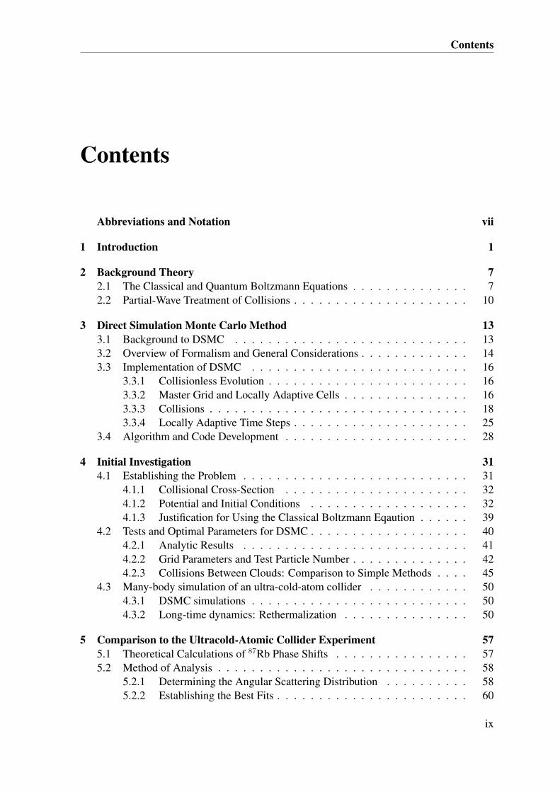
Contents
Abbreviations and Notation vii
1 Introduction 1
2 Background Theory 72.1 The Classical and Quantum Boltzmann Equations . . . . . . . . . . . . . . 72.2 Partial-Wave Treatment of Collisions . . . . . . . . . . . . . . . . . . . . . 10
3 Direct Simulation Monte Carlo Method 133.1 Background to DSMC . . . . . . . . . . . . . . . . . . . . . . . . . . . . 133.2 Overview of Formalism and General Considerations . . . . . . . . . . . . . 143.3 Implementation of DSMC . . . . . . . . . . . . . . . . . . . . . . . . . . 16
3.3.1 Collisionless Evolution . . . . . . . . . . . . . . . . . . . . . . . . 163.3.2 Master Grid and Locally Adaptive Cells . . . . . . . . . . . . . . . 163.3.3 Collisions . . . . . . . . . . . . . . . . . . . . . . . . . . . . . . . 183.3.4 Locally Adaptive Time Steps . . . . . . . . . . . . . . . . . . . . . 25
3.4 Algorithm and Code Development . . . . . . . . . . . . . . . . . . . . . . 28
4 Initial Investigation 314.1 Establishing the Problem . . . . . . . . . . . . . . . . . . . . . . . . . . . 31
4.1.1 Collisional Cross-Section . . . . . . . . . . . . . . . . . . . . . . 324.1.2 Potential and Initial Conditions . . . . . . . . . . . . . . . . . . . 324.1.3 Justification for Using the Classical Boltzmann Eqaution . . . . . . 39
4.2 Tests and Optimal Parameters for DSMC . . . . . . . . . . . . . . . . . . . 404.2.1 Analytic Results . . . . . . . . . . . . . . . . . . . . . . . . . . . 414.2.2 Grid Parameters and Test Particle Number . . . . . . . . . . . . . . 424.2.3 Collisions Between Clouds: Comparison to Simple Methods . . . . 45
4.3 Many-body simulation of an ultra-cold-atom collider . . . . . . . . . . . . 504.3.1 DSMC simulations . . . . . . . . . . . . . . . . . . . . . . . . . . 504.3.2 Long-time dynamics: Rethermalization . . . . . . . . . . . . . . . 50
5 Comparison to the Ultracold-Atomic Collider Experiment 575.1 Theoretical Calculations of 87Rb Phase Shifts . . . . . . . . . . . . . . . . 575.2 Method of Analysis . . . . . . . . . . . . . . . . . . . . . . . . . . . . . . 58
5.2.1 Determining the Angular Scattering Distribution . . . . . . . . . . 585.2.2 Establishing the Best Fits . . . . . . . . . . . . . . . . . . . . . . . 60
ix
Contents
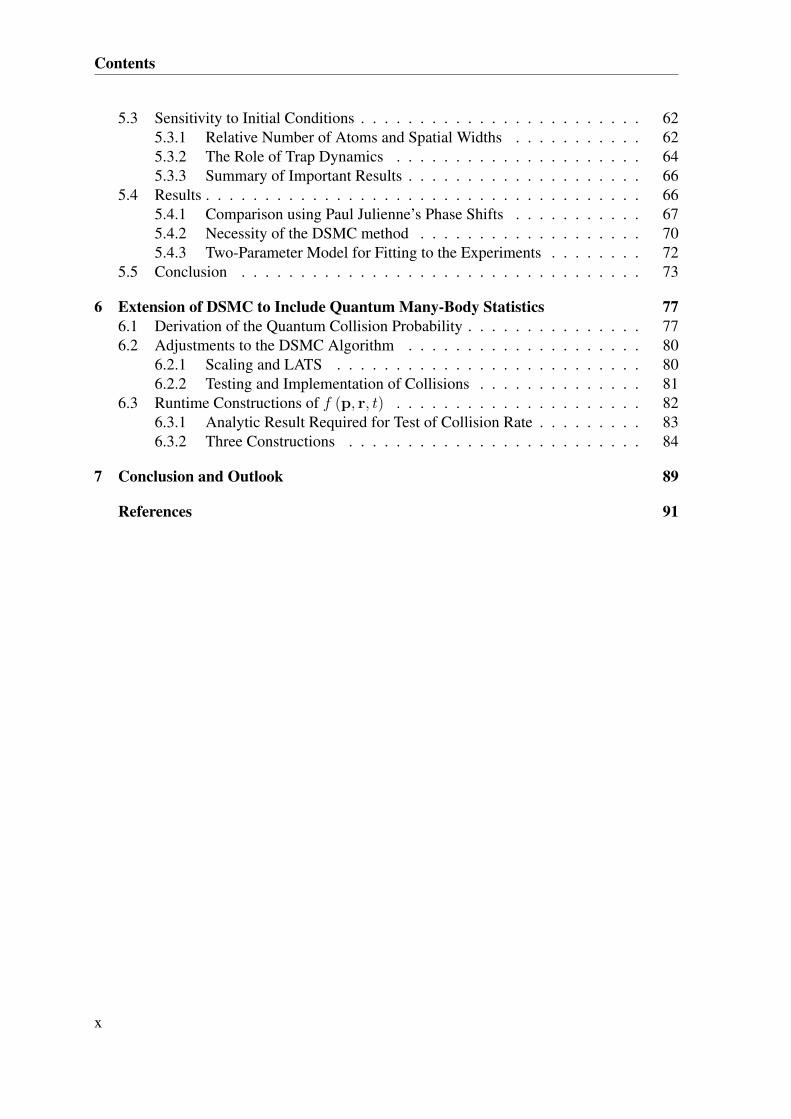
5.3 Sensitivity to Initial Conditions . . . . . . . . . . . . . . . . . . . . . . . . 625.3.1 Relative Number of Atoms and Spatial Widths . . . . . . . . . . . 625.3.2 The Role of Trap Dynamics . . . . . . . . . . . . . . . . . . . . . 645.3.3 Summary of Important Results . . . . . . . . . . . . . . . . . . . . 66
5.4 Results . . . . . . . . . . . . . . . . . . . . . . . . . . . . . . . . . . . . . 665.4.1 Comparison using Paul Julienne’s Phase Shifts . . . . . . . . . . . 675.4.2 Necessity of the DSMC method . . . . . . . . . . . . . . . . . . . 705.4.3 Two-Parameter Model for Fitting to the Experiments . . . . . . . . 72
5.5 Conclusion . . . . . . . . . . . . . . . . . . . . . . . . . . . . . . . . . . 73
6 Extension of DSMC to Include Quantum Many-Body Statistics 776.1 Derivation of the Quantum Collision Probability . . . . . . . . . . . . . . . 776.2 Adjustments to the DSMC Algorithm . . . . . . . . . . . . . . . . . . . . 80
6.2.1 Scaling and LATS . . . . . . . . . . . . . . . . . . . . . . . . . . 806.2.2 Testing and Implementation of Collisions . . . . . . . . . . . . . . 81
6.3 Runtime Constructions of f (p, r, t) . . . . . . . . . . . . . . . . . . . . . 826.3.1 Analytic Result Required for Test of Collision Rate . . . . . . . . . 836.3.2 Three Constructions . . . . . . . . . . . . . . . . . . . . . . . . . 84
7 Conclusion and Outlook 89
References 91
x
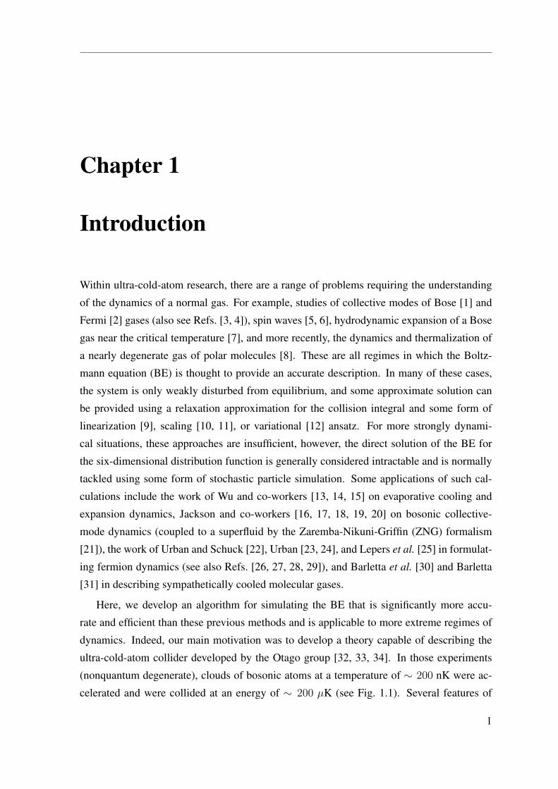
Chapter 1
Introduction
Within ultra-cold-atom research, there are a range of problems requiring the understanding
of the dynamics of a normal gas. For example, studies of collective modes of Bose [1] and
Fermi [2] gases (also see Refs. [3, 4]), spin waves [5, 6], hydrodynamic expansion of a Bose
gas near the critical temperature [7], and more recently, the dynamics and thermalization of
a nearly degenerate gas of polar molecules [8]. These are all regimes in which the Boltz-
mann equation (BE) is thought to provide an accurate description. In many of these cases,
the system is only weakly disturbed from equilibrium, and some approximate solution can
be provided using a relaxation approximation for the collision integral and some form of
linearization [9], scaling [10, 11], or variational [12] ansatz. For more strongly dynami-
cal situations, these approaches are insufficient, however, the direct solution of the BE for
the six-dimensional distribution function is generally considered intractable and is normally
tackled using some form of stochastic particle simulation. Some applications of such cal-
culations include the work of Wu and co-workers [13, 14, 15] on evaporative cooling and
expansion dynamics, Jackson and co-workers [16, 17, 18, 19, 20] on bosonic collective-
mode dynamics (coupled to a superfluid by the Zaremba-Nikuni-Griffin (ZNG) formalism
[21]), the work of Urban and Schuck [22], Urban [23, 24], and Lepers et al. [25] in formulat-
ing fermion dynamics (see also Refs. [26, 27, 28, 29]), and Barletta et al. [30] and Barletta
[31] in describing sympathetically cooled molecular gases.
Here, we develop an algorithm for simulating the BE that is significantly more accu-
rate and efficient than these previous methods and is applicable to more extreme regimes of
dynamics. Indeed, our main motivation was to develop a theory capable of describing the
ultra-cold-atom collider developed by the Otago group [32, 33, 34]. In those experiments
(nonquantum degenerate), clouds of bosonic atoms at a temperature of ∼ 200 nK were ac-
celerated and were collided at an energy of ∼ 200 µK (see Fig. 1.1). Several features of
1

Chapter 1. Introduction
)d()c(
)f()e(
174 µK 225 µK
250 µmExperiment Experiment
Theory Theory
(a)
thermal velocity spread of cloud ~6mm/s
center of mass velocity ~12 cm/s
(b)
scattered atoms
Figure 1.1: Ultra-cold-atom collider: (a) schematic of the precollision ar-
rangement of two clouds at ∼ 200 nK approaching at a collision energy
of ∼ 200µK; (b) schematic of a postcollision system. (c) and (d) experi-
mental images, presented by Thomas et al. [32], of post scattering density
for two collision energies spanning the d-wave shape resonance. (e) and
(f) show our theoretical calculations matching the experimental results us-
ing the direct simulation Monte Carlo (DSMC) method developed in this
thesis. Following the terminology established in experiments, we char-
acterize the collider kinetic energy in temperature units by the parameter
Tcoll ≡ µv2r /2kB, where µ = m/2 is the reduced mass, and vr is the
magnitude of the relative velocity.
2

these experiments make the numerical simulation difficult:
(i) The system is far from equilibrium and accesses a large volume of phase space. A
good representation of each cloud before the collision requires nano-Kelvin energy
resolution, however, during the collision, atoms are scattered over states on the colli-
sion sphere with an energy spread on the order of a milli-Kelvin.
(ii) The collision energies are sufficiently large that an appreciable amount of higher-order
(i.e. beyond s-wave) scattering occurs. In particular, in experiments p-wave scattering
[34] and a d-wave [32] shape resonance have been explored (see Fig. 1.2).
The algorithm we develop is suitable for this regime, and, as shown in Figs. 1.1(c)-1.1(f), it
can provide a quantitative model for the experimental data in Ref. [32]. Feature (i) discussed
above presents a great challenge, and using the traditional Boltzmann techniques employed
to date in ultra-cold-atom research, this would require super computer resources. We show
how to make use of an adaptive algorithm (that adapts both the spatial grid and the times
steps to place resources where needed) to accurately simulate an ultra-cold-atom collider on
commodity personal computer hardware.
We note that, in addition to collider experiments, a capable BE solver would allow the-
oretical studies in a range of areas of emerging interest, such as the turbulence and flow in-
stabilities in the normal phase of a quantum gas. Here, we will focus mostly on the classical
regime where the phase-space density is small compared to unity such that the many-body
effects of Bose-stimulated or Pauli-blocked scatterings are negligible. However, the systems
we consider will be in the quantum collision regime, whereby the thermal de Broglie wave-
length is larger than the typical range of the interatomic potential. Notably, in this regime, the
scattering is wave like, and quantum statistics on the two-body level gives rise to profound
effects in the individual collision processes, even though many-body quantum statistics is
unimportant.
All of the Boltzmann simulations appearing in the ultra-cold-atom literature have been
based on DSMC-like methods, typically employing the algorithm described in Bird’s 1994
monograph [35]. However, a challenging feature of ultracold gases is that the local properties
(e.g., the density) can vary by orders of magnitude across the system, and no single global
choice of parameters for the DSMC can provide a good description across this entire range.
For this reason, we introduce the use of two locally adaptive schemes to allow the system to
refine the description and to allocate more computational resources to regions of high density.
These schemes are as follows: locally adaptive time steps (LATSs) and locally adaptive cells
(LACs). We discuss these, as well as the overall DSMC method, in Chapter 3.
3
Chapter 1. Introduction
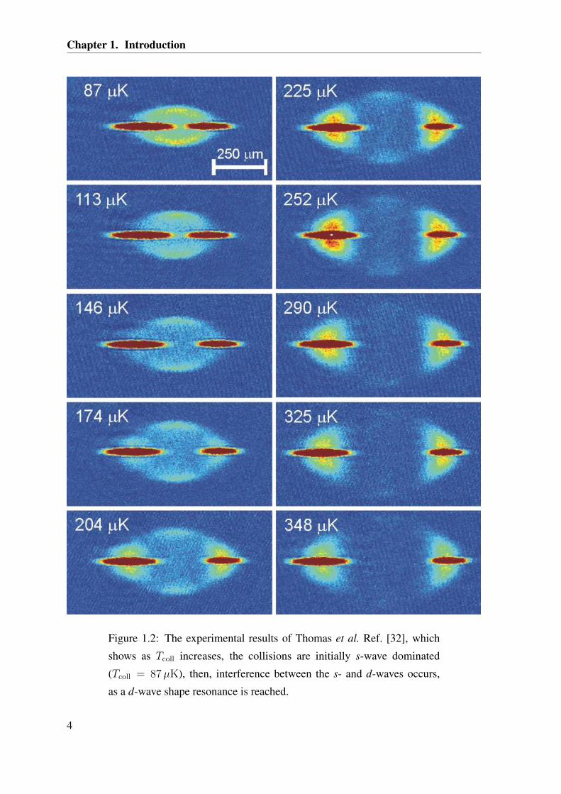
Figure 1.2: The experimental results of Thomas et al. Ref. [32], which
shows as Tcoll increases, the collisions are initially s-wave dominated
(Tcoll = 87µK), then, interference between the s- and d-waves occurs,
as a d-wave shape resonance is reached.
4
In Chapter 4, we establish how to solve the problem of the ultra-cold-atom collider,
and we validate our algorithm using a variety of tests to demonstrate its applicability and
performance. Then, we apply it to the regime of the ultra-cold-atom collider experiments
[32]. Following this, in Chapter 5, we perform a quantitative study of the ultra-cold-atom
collider. Finally, in Chapter 6, we discuss extending the DSMC algorithm to include quantum
many-body statistics.
The work of Chapters 3 and 4 has been published in Physical Review A [36], and, for the
work of Chapter 5, there is a paper in preparation.
5


Chapter 2
Background Theory
Here, we describe the Boltzmann equation and the quantum Boltzmann equation, as well
as, the partial-wave description of the differential cross section. Useful references for the
BE are the books by Huang [37] and Kardar [38], and for the quantum BE and partial-wave
description, the book by Pethick and Smith [39].
2.1 The Classical and Quantum Boltzmann Equations
The quantum BE appears in many fields, and has been labelled with many names, for exam-
ple, the Boltzmann-Uehling-Uhlenbeck, Vlasov-Uehling-Uhlenbeck, Boltzmann-Nordheim,
and Landau-Vlasov equation. Here, we choose to refer to this equation, as the quantum
Boltzmann equation.
The system of interest is a dilute gas of identical atoms, and is described semiclas-
sically by the phase-space distribution function f ≡ f (p, r, t), where f (p, r, t) d3pd3x
is the mean number of atoms in the phase-space volume p → p + (dpx, dpz, dpz) and
r → r + (dx, dy, dz). The quantum BE gives the evolution of the distribution function
[39] [∂
∂t+
p
m· ∇r −∇rU (r, t) · ∇p
]f = I [f ] , (2.1)
where the position-space density of the atoms n (r, t) is given by
n (r, t) =
∫d3p
h3f (p, r, t) . (2.2)
The left-hand side of Eq. (2.1) describes the evolution of atoms under the potential U (r, t).
In general, U (r, t) may contain a mean-field term, e.g.,
UMF (r, t) = 2gn (r, t) , (2.3)
7

Chapter 2. Background Theory
where g = 4π~2asc/m, with asc as the s-wave scattering length, which discussed further in
the next section. However, for our analysis presented here, we only consider the case where
U (r, t) is an external trapping potential.
The collision integral I [f ], accounts for the collisions between atoms, and is given by
I [f ] =1
m
∫d3p1
h3
∫dΩ
dσ
dΩ|p1 − p| [ f ′f ′1 (1± f) (1± f1)︸ ︷︷ ︸
Incoming
− ff1 (1± f ′) (1± f ′1)︸ ︷︷ ︸Outgoing
],
(2.4)
where dσdΩ
is the differential cross section, and f1 ≡ f (p1, r, t), f ′ ≡ f (p′, r, t), etc.
When considering the flow of atoms through phase space due to collisions, I [f ] has
a simple interpretation. The outgoing term in Eq. (2.4) containing ff1 describes binary
collisions of point-like atoms, where the atoms are initially at the phase-space points (p, r)
and (p1, r), and have final states (p′, r) and (p′1, r). During such a collision, total and relative
momenta
P =p + p1
2, P′ =
p′ + p′12
, (2.5a)
pr = p1 − p, p′r = p′1 − p′, (2.5b)
respectively, are constrained by
P = P′, (2.6a)
|pr| = |p′r| , (2.6b)
to ensure conservation of momentum and energy (a geometrical representation of the colli-
sion can be seen in Fig. 2.1). The atomic interactions we wish to describe are contained in
the differential cross section, which describes the angular distribution for scattering events
between pairs of atoms as a function of their relative speed, and Ω is the solid angle formed
by the incoming and outgoing relative momenta.
The incoming term of Eq. (2.4) describes the opposite process where atoms scatter from
(p′, r) and (p′1, r) to (p, r) and (p1, r). The quantum statistics of the atoms is included by the
(1± f ′) (1± f ′1) terms, which account for Bose-stimulated scattering (+) or Pauli blocking
(−).
Neglecting Bose-stimulated scattering, or Pauli blocking, gives the BE, which is appro-
priate for nondegenerate regimes where f 1. In detail, the BE reads[∂
∂t+
p
m· ∇r −∇rU (r, t) · ∇p
]f =
1
m
∫d3p1
h3
∫dΩ
dσ
dΩ|p1 − p| [f ′f ′1 − ff1] , (2.7)
and is the main focus of this thesis, except for the extensions of the DSMC algorithm dis-
cussed in Chapter 6 to describe the quantum BE [Eqs. (2.1) and Eq. (2.4)].
8

2.1. The Classical and Quantum Boltzmann Equations
P = P
p1
p
p1
p
pr
pr
Figure 2.1: Geometrical representation of a binary collision of point-like
particles. During the collision, the total energy and the total momentum of
the pair are conserved. Only the momenta are changed by keeping the total
momentum constant, and rotating the relative momentum vector about its
center [37]. The initial states of the two particles are shown in black, while
the final states are shown in red, while the axes give the momenta in x, y,
and z directions.
9
Chapter 2. Background Theory
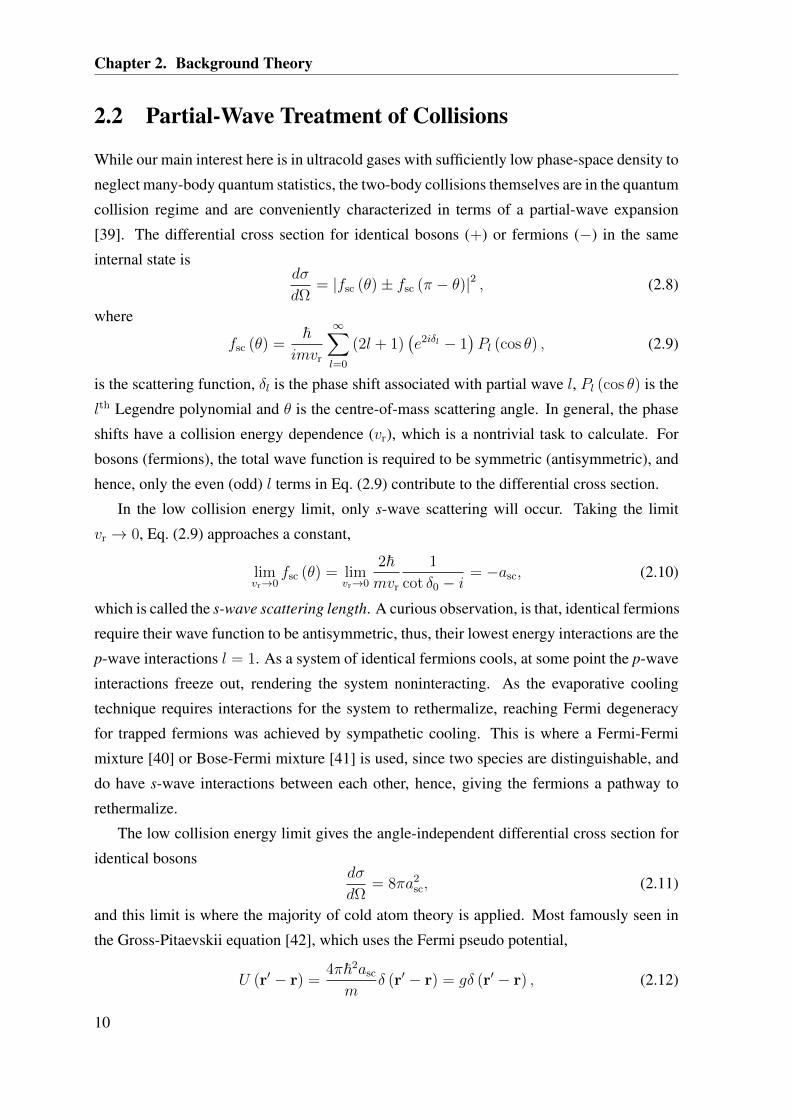
2.2 Partial-Wave Treatment of Collisions
While our main interest here is in ultracold gases with sufficiently low phase-space density to
neglect many-body quantum statistics, the two-body collisions themselves are in the quantum
collision regime and are conveniently characterized in terms of a partial-wave expansion
[39]. The differential cross section for identical bosons (+) or fermions (−) in the same
internal state isdσ
dΩ= |fsc (θ)± fsc (π − θ)|2 , (2.8)
where
fsc (θ) =~
imvr
∞∑
l=0
(2l + 1)(e2iδl − 1
)Pl (cos θ) , (2.9)
is the scattering function, δl is the phase shift associated with partial wave l, Pl (cos θ) is the
lth Legendre polynomial and θ is the centre-of-mass scattering angle. In general, the phase
shifts have a collision energy dependence (vr), which is a nontrivial task to calculate. For
bosons (fermions), the total wave function is required to be symmetric (antisymmetric), and
hence, only the even (odd) l terms in Eq. (2.9) contribute to the differential cross section.
In the low collision energy limit, only s-wave scattering will occur. Taking the limit
vr → 0, Eq. (2.9) approaches a constant,
limvr→0
fsc (θ) = limvr→0
2~mvr
1
cot δ0 − i= −asc, (2.10)
which is called the s-wave scattering length. A curious observation, is that, identical fermions
require their wave function to be antisymmetric, thus, their lowest energy interactions are the
p-wave interactions l = 1. As a system of identical fermions cools, at some point the p-wave
interactions freeze out, rendering the system noninteracting. As the evaporative cooling
technique requires interactions for the system to rethermalize, reaching Fermi degeneracy
for trapped fermions was achieved by sympathetic cooling. This is where a Fermi-Fermi
mixture [40] or Bose-Fermi mixture [41] is used, since two species are distinguishable, and
do have s-wave interactions between each other, hence, giving the fermions a pathway to
rethermalize.
The low collision energy limit gives the angle-independent differential cross section for
identical bosonsdσ
dΩ= 8πa2
sc, (2.11)
and this limit is where the majority of cold atom theory is applied. Most famously seen in
the Gross-Pitaevskii equation [42], which uses the Fermi pseudo potential,
U (r′ − r) =4π~2asc
mδ (r′ − r) = gδ (r′ − r) , (2.12)
10

2.2. Partial-Wave Treatment of Collisions
for the atom-atom interactions, where δ (r′ − r) is the Dirac delta-function. Here, we will
use this low energy limit for simple tests in Chapter 4.
The total cross section σ (vr), is obtained by integrating over only half the total solid
angle, to avoid double counting, and is given by the sum of the total cross sections for each
partial-wave,
σ (vr) =∞∑
l=0
σl (vr) , (2.13)
where
σl (vr) = 32π (2l + 1)
(~ sin δlmvr
)2
. (2.14)
11

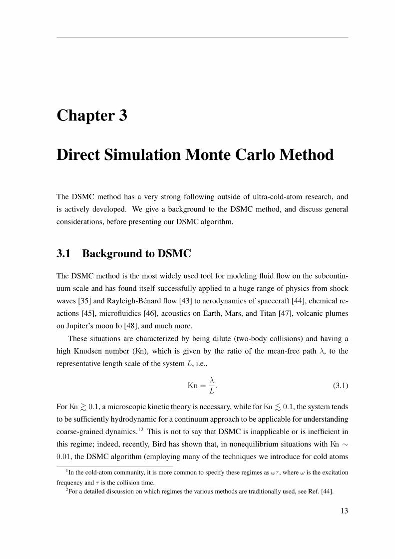
Chapter 3
Direct Simulation Monte Carlo Method
The DSMC method has a very strong following outside of ultra-cold-atom research, and
is actively developed. We give a background to the DSMC method, and discuss general
considerations, before presenting our DSMC algorithm.
3.1 Background to DSMC
The DSMC method is the most widely used tool for modeling fluid flow on the subcontin-
uum scale and has found itself successfully applied to a huge range of physics from shock
waves [35] and Rayleigh-Bénard flow [43] to aerodynamics of spacecraft [44], chemical re-
actions [45], microfluidics [46], acoustics on Earth, Mars, and Titan [47], volcanic plumes
on Jupiter’s moon Io [48], and much more.
These situations are characterized by being dilute (two-body collisions) and having a
high Knudsen number (Kn), which is given by the ratio of the mean-free path λ, to the
representative length scale of the system L, i.e.,
Kn =λ
L. (3.1)
For Kn & 0.1, a microscopic kinetic theory is necessary, while for Kn . 0.1, the system tends
to be sufficiently hydrodynamic for a continuum approach to be applicable for understanding
coarse-grained dynamics.12 This is not to say that DSMC is inapplicable or is inefficient in
this regime; indeed, recently, Bird has shown that, in nonequilibrium situations with Kn ∼0.01, the DSMC algorithm (employing many of the techniques we introduce for cold atoms
1In the cold-atom community, it is more common to specify these regimes as ωτ , where ω is the excitation
frequency and τ is the collision time.2For a detailed discussion on which regimes the various methods are traditionally used, see Ref. [44].
13

Chapter 3. Direct Simulation Monte Carlo Method
here) can be more accurate and efficient than Navier-Stokes methods, while also providing
details of the microscopic (subcontinuum) dynamics [49]. We also note that the consistent
Boltzmann algorithm [50] was developed by making an adjustment to the DSMC algorithm,
where the positional shifts of the atoms due to collisions are taken into account, thus, giving
the correct hard-sphere virial. This allows for exploration into even lower Kn and has been
explored in the context of quantum nuclear flows [51, 52].
For reference, cold-atom experiments often operate in the collisionless regime (Kn >
1), however, values of Kn ∼ 0.01 have been explored, e.g., the above-critical temperature
collective modes of a 23Na gas studied by Stamper-Kurn et al. [4] had Kn ∼ 0.1; Shvarchuck
et al. [1] studied the hydrodynamical behavior of a normal 87Rb gas in which Kn ∼ 0.02−0.5.
3.2 Overview of Formalism and General Considerations
In the DSMC method, the distribution function is represented by a swarm of test particles,
f (p, r, t) ≈ αh3
NT∑
i=1
δ [p− pi (t)] δ [r− ri (t)] , (3.2)
where α = NP/NT is the ratio of physical atoms (NP) to test particles (NT). These test
particles are evolved in time in such a manner that f (p, r, t) evolves according to the BE.
The basic assumption of DSMC is that the motion of atoms can be decoupled from colli-
sions on time scales much smaller than the mean-collision time. In practice, this means that
a simulation is split up into discrete time steps ∆t, during which, the test particles undergo a
collisionless evolution, then, collisions between test particles are calculated.
The relation of the test particles to physical atoms is apparent in Eq. (3.2) when α = 1,
but, in general, they are simply a computational device for solving the BE. In many con-
ventional applications of DSMC, good accuracy can be obtained with α 1 (i.e., each is
a super particle representing a larger number of physical atoms), however, in our applica-
tions to the nonequilibrium dynamics of ultracold gases, we often require α 1. Increasing
the number of particles improves both the accuracy and the statistics of the simulation, and
in highly nonequilibrium situations, it can be essential to have a large number of particles.
The DSMC algorithm is designed so that the number of computational operations per time
step scales linearly with the number of particles, i.e., O (NT). The recent work of Lepers et
al. [25] departs from DSMC by using a stochastic particle method similar to that developed
in nuclear physics for the simulation of heavy-ion collisions [53, 54], which tests if two par-
ticles are at their closest approach in the present time step, causing the algorithm to scale as
14

3.2. Overview of Formalism and General Considerations
O (N 2T). These methods have been reformulated in terms of DSMC by Lang et al. [55]. We
typically use NT = 105 − 107 test particles, and, by the various improvements we describe
below, in most cases we consider here, we can obtain accuracy to within 1%.
As pointed out in Sec. 2.1, the BE has a simple interpretation in terms of the flow of atoms
through phase space. Hence, the collisionless evolution of the test particles is performed by
solving Newton’s laws for the potential U (r, t), and collisions are governed by the collision
integral [Eq. (2.7)]. The collisions are implemented probabilistically (see Sec. 3.3.3) using
a scheme that requires the particles to be binned into a grid of cells in position space. This
serves two purposes: (i) It allows for the sampling of the distribution function, and (ii) it
establishes a computationally convenient mechanism for determining which particles are in
close proximity. Thus, the accuracy of DSMC depends on the discretization of the problem,
the cell size, the time step, and NT. It has been shown to converge to the exact solution of
the BE in the limit of infinite test particles, vanishing cell size, and vanishing time step [56].
In the original DSMC algorithm [35], a test particle may collide with any other particle
within the cell. This coarse grains position and momentum correlations, such as vorticity, to
be the length scale of the cells, as observed by Meiburg [57]. If the cells are not small enough,
this transfer of information across a cell could lead to nonphysical behavior. To combat this,
we have employed a nearest neighbor collision (NNC) scheme [58] outlined in Sec. 3.3.3,
where the collision partner of a particle must be chosen from the nearest neighbors. Although
a NNC scheme alleviates this problem, the cell sizes still must be small in comparison to the
local mean-free path and the length scale over which the density varies for accurate sampling.
The time step of the simulation must also be small in comparison to the smallest local
mean-collision time to ensure the validity of the basic assumption of DSMC and that physical
atoms do not propagate further than the local mean free path before colliding. To ensure this
(and for added efficiency), we implement LATSs [58] where, instead of a single global time
step, the time step can vary over the whole system, adapting to the local environment.
Finally, we note that the most useful choice of computational units (for the harmonic
potential) for length, time, and energy, are respectively given by
x0 =
√~mω
, t0 =1
ω, ε0 = ~ω, (3.3)
where ω is chosen to be ωx, ωy, or ωz.
15

Chapter 3. Direct Simulation Monte Carlo Method
3.3 Implementation of DSMC
Here, we consider the basic implementation of DSMC; a collisionless evolution followed
by a collision step where test particles are binned in position space and collisions between
them are implemented stochastically via a collision probability. We also discuss the various
adaptive schemes we employ for better accuracy and efficiency, while retaining the desired
linear scaling of the computational complexity with test particle number.
3.3.1 Collisionless Evolution
The collisionless evolution is performed by a second-order symplectic integrator [59, 18],
which updates the phase-space variables of the ith test particle in three steps:
qi = ri (t) +∆t
2mpi (t) , (3.4a)
pi (t+ ∆t) = pi (t)−∆t∇qiU (qi, t) , (3.4b)
ri (t+ ∆t) = qi +∆t
2mpi (t+ ∆t) . (3.4c)
Symplectic integrators have the properties of conserving energy and phase-space volume
over long periods of time. The conservation of phase-space volume is particularly desirable
for fermionic simulations, since it assists in ensuring the Pauli exclusion principle is not
violated during the collisionless evolution.
3.3.2 Master Grid and Locally Adaptive Cells
To perform collisions, we must first bin the test particles into a grid of cells according to their
position. Collision partners are then selected from within each cell. In general, the binning
occurs in up to two levels: (i) the master grid on which each master cell is a rectangular
cuboid of equal size [see Fig. 3.1(a)] and (ii) the adaptive subdivision of the master cells into
smaller LAC subcells dependent on the number of particles in the parent master cell [see
Fig. 3.1(b)], which is an optional refinement. The use of several LAC schemes in DSMC
is discussed in Ref. [35]. It is a useful refinement to the algorithm for applications to cold-
atom systems, because these typically have large variations in density (such a scheme has
been employed in Ref. [60] to account for the large change in density during evaporative
cooling of a cloud of cesium atoms). We now discuss these levels in further detail.
At the beginning of the collision step, the grid of master cells is chosen to ensure all
particles are held within its boundaries [see Fig. 3.1(a)]. We choose to keep the size of the
master cells in each direction constant in time so that if the particles spread out further in
16
3.3. Implementation of DSMC
(a)
master cells
∆x
∆y
∆x
∆y
(b)
adaptive subdivisionof master cells
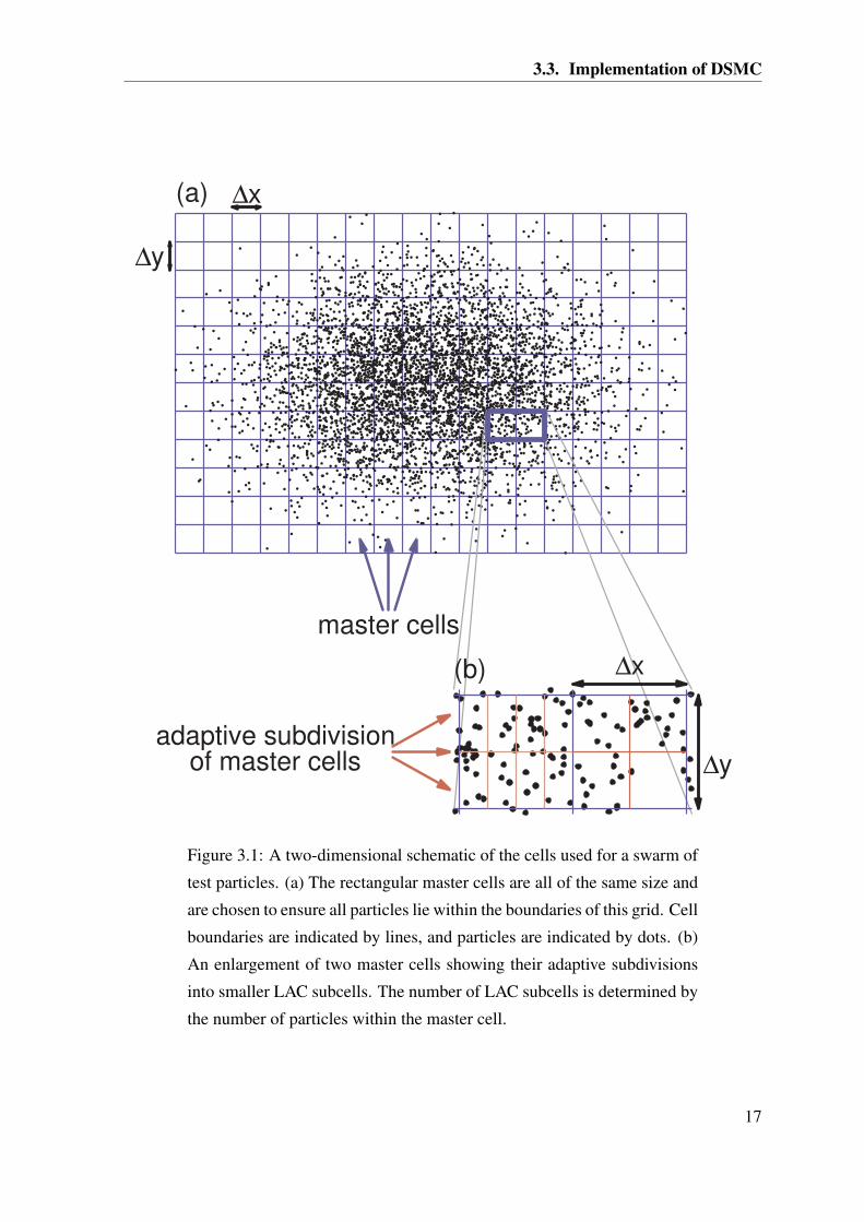
Figure 3.1: A two-dimensional schematic of the cells used for a swarm of
test particles. (a) The rectangular master cells are all of the same size and
are chosen to ensure all particles lie within the boundaries of this grid. Cell
boundaries are indicated by lines, and particles are indicated by dots. (b)
An enlargement of two master cells showing their adaptive subdivisions
into smaller LAC subcells. The number of LAC subcells is determined by
the number of particles within the master cell.
17
Chapter 3. Direct Simulation Monte Carlo Method
space during the simulation, we add extra cells rather than changing the size of the cells. The
particles are then binned into these master cells, and the number of particles in each cell Nc
is stored.
For adaptive subdivision, each master cell is considered in turn, and the particles are
binned further into a grid of smaller LAC subcells according toNc [see Fig. 3.1(b)]. Because
the number of collisions within a cell increases with density (i.e., number of particles), the
subdivision of highly occupied master cells gives a finer resolution of spatial regions where
the local collision rate is highest and, hence, more accurate simulations.
Our subdivision procedure aims to produce cells in which the average number of particles
is close to some threshold value Nth for which the choice of is discussed in Sec. 4.2.2. In
our algorithm, we do this by finding the integer l such that Nc/2l is closest to, but not less
than, Nth. The master cell is then subdivided into 2l subcells, while giving no preference
to any direction in this subdivision. We choose this division scheme over more complicated
schemes, as when additionally implementing LATSs, the protocol for dynamically changing
grids becomes simpler.
We have adopted the notation of specifying quantities pertaining to a particular cell by
a subscript c. In what follows, when referring to cells, we will mean finest level of cells,
i.e., the LAC subcells or master cells otherwise. We do not explicitly label the cells, indeed,
this is to partly emphasize that the calculations performed in each cell are independent of
other cells. Thus, the algorithm is intrinsically parallel and is suitable for implementation on
parallel platforms (e.g., see Ref. [46]).
3.3.3 Collisions
Number of Tested Collisions
The BE describes the evolution of the continuous distribution f (p, r, t). However, the re-
placement of f (p, r, t) with a swarm of test particles introduces fluctuations that do not
correspond to physical fluctuations when NP 6= NT. As a result, hydrodynamic quantities
are required to be obtained from the averages of mechanical variables, not the average of
their instantaneous values [61].
In these stochastic particle methods, the collisions of test particles inherently average the
instantaneous values of the collision rate. This leads to a biasing of the total collision rate
when cells have low occupation numbers (see Fig. 3.2).
The probability distribution of the Nc test particles within a cell is well approximated by
18

3.3. Implementation of DSMC
104
105
106
107
−0.10
−0.05
0
0.05
0.10
0.15
Rel
ati
ve
Err
or
NT
M ac Theory
M ac
M bc Theory
M bc
M bc No Fix
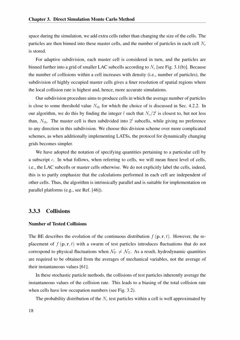
Figure 3.2: Relative error of the numerical total collision rate in the case
of the equilibrium distribution [Eq. (4.7)] for the choices of Mc, where the
error bars indicate the standard deviations of 500 averages. Here, the orig-
inal DSMC algorithm is implemented with NT = 107 and bin parameter
[Eq. (4.16)] γ = 0.2. The choice Mac is seen to diverge for low NT as Nc
in Eq. (3.8) becomes appreciable, which agrees well with the theoretically
calculated error (Mac theory) using Eq. (3.8). Using M b
c removes this di-
vergence, and the error is seen to agree well with the expected error for this
discretization (M bc theory). The final data set (M b
c no fix) demonstrates the
error that arises when Mc having non integer values after rescaling, is not
accounted for [i.e., not including the ceiling function in Eq. (3.14)]. The
system parameters are given in Fig. 4.7. [See Sec. 4.2 for the details of the
DSMC simulation].
19

Chapter 3. Direct Simulation Monte Carlo Method
the Poisson distribution [62] of which the variance is equal to the mean, i.e.,
δN2c = N2
c −Nc2
= Nc, (3.5)
where δNc = Nc−Nc. Note that, formally, the correct number of collisions to test (given by
elementary scattering theory and the derivation of the collision probability from the collision
integral (2.7) via the Monte Carlo integration [18]) is
Mac =
N2c
2. (3.6)
However, with Poissonian fluctuations in Nc, we find that the mean collision rate is R ∝Mc ∼ Nc
2+Nc (but should be∝ Nc
2). Thus, Poissonian fluctuations can become important
when the number of test particles per cell is small. However, the effect of fluctuations from
the finite-test particle number can be bypassed (e.g., see Ref. [49]) by instead using the
number of possible pairs of test particles,
M bc =
Nc (Nc − 1)
2, (3.7)
which we have employed in this work.
To understand the difference in detail, we note that the average calculated by the DSMC
simulation (denoted by the asterisks) for Eq. (3.6) is
N2c
∗= Nc
2+Nc − P1, (3.8)
where P1 is the probability ofNc = 1 (as the simulation ignores cells withNc = 1, for which
no collisions occur, and this must be subtracted from the average). While, for expression
(3.7),
Nc (Nc − 1)∗
= Nc2, (3.9)
which gives the correct total collision rate for the physical system as seen in Fig. 3.2.
Collision Probability and Scaling
The collision probability for a pair of test particles i and j in a cell of volume ∆Vc is given
by
Pij = α∆t
∆Vcvrσ (vr) . (3.10)
This collision probability can be derived from the collision integral (2.7) via the Monte Carlo
integration [18] (see also Sec. 6.1), the kinetic arguments [35], or the elementary scattering
theory [54]. The correct collision rate is established by testing
Mc =Nc (Nc − 1)
2(3.11)
20
3.3. Implementation of DSMC
collisions in the cell. This is inefficient as the number of operations scales as N 2T, and the
collision probability may be far less than 1. However, within a cell, the collision probabilities
and the number of tested collisions can be rescaled by a single parameter Λ such that the
number of operations scales as NT [35],
Pij → Pij =PijΛ, (3.12a)
Mc → Mc = McΛ, (3.12b)
and still converge to the same BE evolution. Here, Λ is chosen to be
Λ =
⌈Mcα
∆t∆Vc
[vrσ (vr)]max
⌉
Mc
, (3.13)
where [vrσ (vr)]max is the maximum of this quantity over all pairs of particles in the cell
and dxe denotes the ceiling function. This corresponds to Bird’s proposal of using Λ =
max Pij [35], while we ensure that Mc is an integer and at least one collision is tested
(Fig. 3.2 demonstrates the reduction in collision rate, if this is not taken into account). With
this choice of scaling, the maximum collision probability within the cell is less than or equal
to 1, but is expected to be close to 1, and the number of collisions that need to be tested is
reduced to
Mc =
⌈Nc − 1
2nc∆t [vrσ (vr)]max
⌉, (3.14)
where
nc = αNc/∆Vc, (3.15)
is the average density in the cell.
This enhancement of efficiency is often missed by other stochastic particle methods, or
the collisions are adjusted in some other manner. For example, Tosi et al. [27] introduced
a scheme for fermions where collision pairs with small classical collision probability were
neglected.
Nearest Neighbor Selection of Collision Partners
We employ a NNC scheme to combat discretization effects from finite cell sizes, in particular,
the so-called transient adaptive subcell (TASC) scheme [58]. Simple sorting of the test
particles for the nearest neighbors scales quadratically with the particle number. The TASC
sorting scheme retains linear scaling, but it does not guarantee the exact nearest neighbor.
The basic TASC scheme is to further bin the particles into subcells within the cell [see
Figs. 3.3(a) and 3.3(b)], the number of which is roughly equal to Nc. In our case, the number
21
Chapter 3. Direct Simulation Monte Carlo Method
collision pair
(a)
transient sub-cells
(b)central sub-cell
layer 1layer 2layer 3
collision pair
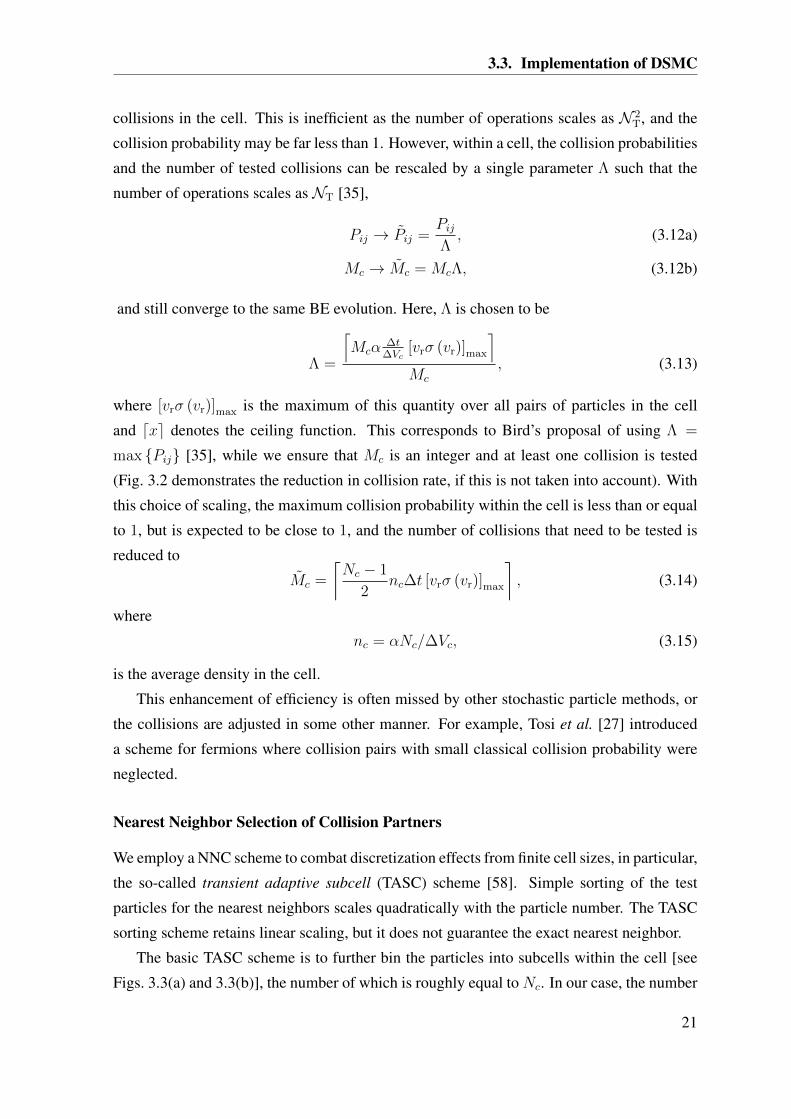
Figure 3.3: A two-dimensional schematic of how collisions are performed
within the TASC scheme. A single cell (outer boundary line) and the
distribution of test particles (black dots) are shown in (a) and (b) for two
different random collisions. The finer grid of internal lines represents the
boundaries of the TASC subcells. The first particle of the collision pair
is selected at random from all the particles in the cell. In (a), the first
particle occupies a TASC subcell that contains other particles, and the
second participant in the collision is chosen at random from these other
particles. In (b), the first particle (which occupies the central subcell) is
the sole occupant of a TASC subcell. In this case, we check to see if there
are any particles in layer 1, and if so, the collision partner is chosen at
random from these other particles. If there were no particles in layer 1, we
would then check layer 2, and so on.
22

3.3. Implementation of DSMC
of subcells in each direction is equal and is given by b 3√Ncc (with bxc as the floor function).
When a particle is randomly picked for a collision, its collision partner is established by
looking within the immediate TASC subcell [Fig. 3.3(a)], and if not found [Fig. 3.3(b)], each
layer starting closest to the particle is searched for other particles. If a layer contains more
than one particle, the collision partner is randomly chosen from that set to avoid any biasing.
This reduces the distance between colliding pairs significantly and may be decreased even
more by increasing NT.
We use this procedure to select each of the Mc pairs of particles for testing if a collision
occurs. We also ensure a particle does not undergo a second collision in the same time step.
Testing and Implementation of Collisions
For each of the pairs, the collision goes ahead if R < Pij , where R is a random number
uniformly distributed between 0 and 1. As the BE describes binary collisions of point-
like atoms that conserve total energy and momentum, only the momenta are changed by
keeping the total momentum constant, and the relative momentum vector is rotated about its
centre (see Fig. 2.1 or Fig. 3.4). The scattering angles φ and θ, are determined by using an
acceptance-rejection Monte Carlo algorithm for the differential cross section.
The final momenta of the test particles are given by
p′ = P +p′r2, (3.16a)
p′1 = P− p′r2, (3.16b)
hence, we need to determine p′r in the reference frame of the simulation.
In the centre-of-mass reference frame shown in Fig. 3.4, p′r is given by a rotation about
origin (centre of the relative momentum),
p′rcom = pr
sin θ cosφ
sin θ sinφ
cos θ
. (3.17)
To transform to the reference frame of the simulation, two rotations are required, which
are defined by the angles φ′ and θ′. We take θ′ to be the angle between pr and the pz axis
in the simulation reference frame, and φ′ to be the azimuthal angle (i.e., how φ and θ are
defined in the centre-of-mass frame Fig. 3.4). Thus, p′r is rotated about the px axis, then,
about the pz axis by RzRx, where
23

Chapter 3. Direct Simulation Monte Carlo Method
θ
φ
pz
py
px
pr
Figure 3.4: In the centre-of-mass reference frame, where the relative mo-
menta initially points along the pz axis, the collision causes the relative
momenta to be rotated about its centre to the new relative momenta p′r.
Rx =
1 0 0
0 cos θ′ sin θ′
0 − sin θ′ cos θ′
, Rz =
sinφ′ cosφ′ 0
− cosφ′ sinφ′ 0
0 0 1
. (3.18)
In terms of the components of pr = (pa, pb, pc), this gives
RzRx =1
prpd
prpb papc pdpa
−prpa pbpc pdpb
0 −p2d pdpc
, (3.19)
where p2d = p2
a + p2b .
3 Thus, in the simulation reference frame,
p′r =1
pd
sin θ (prpb cosφ+ papc sinφ) + pdpa cos θ
sin θ (pbpc sinφ− prpa cosφ) + pdpb cos θ
pd (pc cos θ − pd sin θ sinφ)
. (3.20)
3In the special case where θ′ = 0, we take Eq. (3.19) to be the identity, i.e., φ′ = π/2. In simulations, the
identity is used when pd ≤ eps, where eps is the numerical precision.
24

3.3. Implementation of DSMC
3.3.4 Locally Adaptive Time Steps
All of the preceding aspects of our implementation of DSMC can be performed with the
single global time step ∆t for all cells such that the evolution of the system is simulated at
the times tk = k∆t, with k as an integer. At each of these steps, the collisionless evolution is
performed, then, is followed by the collision step [see Fig. 3.5(a)]. However, if there is large
variation in the properties over the system, the use of a single time step can be inefficient,
as it may be much smaller than required for low-velocity or low-density regions. This has
been addressed by a recent improvement to the DSMC algorithm [58], where a local time
step was introduced for the collision step. Performing the collision step is computationally
expensive, so this improvement can lead to a great increase in the efficiency of calculations.
With the use of LATSs, there are two time steps of importance for each cell: (i) The
global time step δti, which is the fundamental increment of time in all cells of the system.
The global time after k steps is specified as
tg =k∑
i=1
δti, (3.21)
and during each increment of δti, collisionless evolution is performed [i.e., Eqs. (3.4a)−(3.4c)
with ∆t→ δti]. (ii) The local time step for the cell δtc, which is the desirable time scale for
performing collisions in this particular cell. Note δti = minδtc, i.e., we choose the global
time step to be the smallest value of δtc over all cells in the system at the end of each step.4
A collision step is performed at the global time step when, at least, a time of δtc has
passed since the last collision step for the cell under consideration [see Fig. 3.5(b)]. To
implement this, we introduce a cell timer tc, indicating the time up to which collisions have
been accounted for in the cell. In general, tc < tg and is incremented by δtc during each
collision step. Performing collisions in this way ensures that tc is within δtc of tg at all
times,5 and at the end of the simulation, all tc are updated to the final time by performing
collisions with δtc = tg − tc.In our simulations, δtc is chosen to be small compared to the relevant collision and transit
4If δti is sufficiently large that the accuracy of the collisionless evolution is compromised, δti is split into
smaller increments for this evolution.5If a cell becomes unpopulated (Nc = 0), tc may not have been updated such that tc = tg before the
test particles leave the cell, which decreases the collision rate. However, δtc is chosen such that this effect is
negligible.
25

Chapter 3. Direct Simulation Monte Carlo Method
collisionless evolution
t1 = δt
collisionless evolution
t2 = 2δt
collisionless evolution
t3 = 3δt
collisionless evolution
t4 = 4δt
collisionless evolution
t5 = 5δt
collisionless evolution
t6 = 6δt
collisionless evolution
t7 = 7δt
t0 = 0
δtc
′
δtc
′′
δtc
′′′
δtc
′′′′
tc=0
tc = δt
c
′
tc = δt
c
′+ δt
c
′′
tc = δt
c
′+ δt
c
′′+ δt
c
′′′
update cell timer
update cell timer
update cell timer
collision step ∆t = δtc
′
collision step ∆t = δtc
′′
collision step ∆t = δtc
′′′
δtc
′ δt
c
′′
δtc
′′ δt
c
′′′
δtc
′′′ δt
c
′′′′
tim
e
(b)
collisionless evolution
t1 = ∆t
collisionless evolution
t2 = 2∆t
t0 = 0
collision step
collision step
tim
e(a)
Figure 3.5: An example of the sequence of steps in a DSMC evolution. (a)
A simple DSMC scheme where the whole system evolves according to a
single global time step ∆t. (b) An example of a cell using a LATS. In this
example, the global time step (δt) is held constant, while the local time
step (δtc) is shown to vary. Collisionless evolution occurs at each global
time step. A collision step is performed at the global step when, at least,
δtc has passed since the last collision step. At global time t3, we show a
collision step, at which the local time counter (tc) is updated and a new
local time step (δt′′c ) is established. Here, the local time step decreases,
showing two further collision steps that follow shortly after the first.
26

3.3. Implementation of DSMC
times of the cell. In detail, these time scales,
τ collc =
[ncvrσ (vr)
]−1
, (3.22a)
τmaxc = nc [vrσ (vr)]max
−1 , (3.22b)
τ trc = min
∆xcvx
,∆ycvy
,∆zcvz
, (3.22c)
are the mean-collision time, the maximum collision time, and the mean transit times of the
cell, respectively. These expressions are evaluated at the end of each collision step, and the
mean speeds (vx, vy, vz) are given by averaging over all the test particles within the cell,
while vrσ (vr) is the average of vrσ (vr) over the particles tested for collisions. The cell
widths (∆xc,∆yc,∆zc) correspond to the cell under consideration [e.g., ∆xc is the LAC
subcell x width, and the master bin width (∆x) otherwise].
In terms of these time scales, we take
δtc = minηcollτ
collc , ηmaxτ
maxc , ηtrτ
trc
, (3.23)
where ηcoll, ηmax, and ηtr are constants less than unity. At the end of each collision step, δtcis reset by Eq. (3.23). Whenever δtc is established without performing a collision step, i.e.,
beginning of the simulation or when the LAC subcells are collapsed or expanded, we take it
to be
δtc = minηmaxτ
maxc , ηtrτ
trc
. (3.24)
For the accurate simulation of dynamics, it is required that δtc τ collc as well as δtc
τ trc . We also require that it is unlikely for an atom to undergo multiple collisions in a collision
step (accounted for by τmaxc ). These requirements are ensured by the constants ηcoll, ηmax,
and ηtr, which are optimized for the desired accuracy.
Care has to be taken when the LATS scheme is implemented in conjunction with the
LAC scheme, as the cells can change dynamically during the evolution (cells can be resized,
can be added or can be removed). Our procedure for dealing with dynamically changing
LAC subcells is as follows: As each master cell is considered in turn, if the number of
LAC subcells changes, a new layout of LAC subcells must be established. If the number
of these subcells increases, then each of these new cells inherits the tc of the original cell.
Alternatively, if the number of subcells decreases, then the new cells are formed by merging
old cells. In general, the values of tc for each of the cells to be merged are different, and
we take the new value of tc to be the largest of these. This requires tc of the old cells to be
updated to the new tc, thus, collision steps are performed within the old cells before merging,
using the time difference.
27

Chapter 3. Direct Simulation Monte Carlo Method
When the LAC scheme is implemented with small threshold numbers (e.g., Nth < 5)
and the number of test particles is large (NT > 106), it can become inefficient to implement
LATSs in conjunction with the LAC subcells. In such regimes, very dense grids of LAC
subcells typically arise, for which the computational intensity of the LATS and memory
requirements become too great. Furthermore, small cell sizes lead to excessively small time
steps (e.g., τ trc is proportional to the cell size), which further reduces the algorithm efficiency.
In these cases, it is more efficient to implement the LATS scheme for the master cells (i.e.,
only the master cells have a time counter and desired time step) and implement collisions in
all the LAC subcells using that same desired time step.
3.4 Algorithm and Code Development
The algorithm and code to perform these DSMC calculations was developed over the course
of a year. In that time, our initial algorithm, based on the work of Jackson and Zaremba
[18] was converted from MATLAB to C programming language, and parallelized. Many
problems with the Jackson and Zaremba algorithm were identified, understood, and solved,
by experimentation and finding relevant literature. Most problems were in relation to sim-
ulating far from equilibrium systems, which the Jackson and Zaremba algorithm was not
developed with this in mind. However, there were two crucial problems: the choice of the
number of tested collisions (see Sec. 3.3.3), and a problem in relation to implementing quan-
tum many-body statistics that we discuss in detail in Chapter 6. Both of these problems, can
significantly damage the quality of the simulation.
The final DSMC algorithm, which we presented in this chapter, evolved after testing
many different possible routines and subroutines, taking into consideration speed and mem-
ory constraints. We now briefly outline our implementation of this DSMC algorithm in C
language. While, a significant amount of work has been simultaneously undertaken on a
quantum DSMC implementation, we only seek to outline an algorithm in Chapter 6, as we
have discovered, such an algorithm merits a significant study in its own right.
The main routine is split into three elements that are required to be executed in serial,
and are repeated for each time step of the simulation,
(i) Collisionless evolution.
(ii) Establishing the master grid and binning test particles into it.
(iii) Performing collisions.
Element (i) is the implementation of Eqs. (3.4a)−(3.4c), which is easily parallelized, and is
28
3.4. Algorithm and Code Development
fast. As for element (ii), the master grid from the previous time step must be expanded if the
test particles have evolved outside its boundaries. The master grid holds all the information
about the LAC subcells within each master cell (or itself, if the LAC scheme is not imple-
mented), i.e., how many in each direction, cell time steps, cell time counters, etc. It also
holds the information of which test particles are within each master cell. This has to be es-
tablished each time step, where the cell position of each test particle is established, and they
are sorted into the cells. Components of this routine are not parallelizable, and in element
(ii), there can be large manipulation of memory, causing it to take as long as element (iii).
The last element is the most difficult and intricate, and is usually the most computa-
tionally intensive. Thankfully, performing collisions in each master cell is independent of
the other master cells. Thus, parallelizing this element is straightforward, by passing each
thread a proportion of the master cells. As each master cell is considered, it must be deter-
mined if the layout of LAC subcells needs to be changed. If it does, then, the cells must be
merged or subdivided, where the most difficult part is dealing with redistributing the time
counters and time steps of each LAC subcell (see Sec. 3.3.4). Then, test particles are binned
into the LAC subcells, using the routines for the master cell binning. From here, each LAC
subcell is considered in turn, and the collisions are finally calculated if the time counter of
the cell has fallen behind the global time by its time step. If it has, collisions are calculated,
where the number of collisions and collision probabilities are given by Eqs. (3.12). This
requires establishing the TASC subcells, where the test particles are binned into a grid of
TASC subcells using the routines for the master cell binning. From this grid, the nearest
neighbors are selected. If the collision goes ahead, the momenta of the colliding particles are
adjusted according to Eqs. (3.16), and Eq. (3.20).
29

Chapter 4
Initial Investigation
Before we can perform DSMC simulations, the problem must be established by choosing
inputs that suitably describe the ultra-cold-atom collider experiment [32], and justifying the
neglect of the effect quantum statistics on scattering (Bose-stimulated scattering or Pauli-
blocking). This is the purpose of the first section of this chapter.
In the ultracold gas community, with only a few exceptions, careful studies on the per-
formance of DSMC, and other stochastic particle methods, are not presented along side the
studies employing these methods. One of the purposes of this work was to establish the
accuracy of DSMC, and, as noted in Sec. 3.3.3, a poor implementation of DSMC will result
in significant error. To quantify the accuracy of the DSMC simulations, the second section
develops tests relevant to ultracold systems, and for the particular case of colliding clouds,
our DSMC algorithm is compared to highly accurate pseudo-spectral methods in a simplified
case, finding excellent agreement.
Finally, we demonstrate the simulation of the ultra-cold-atom collider with the full energy
and angular-dependent-scattering cross section, and consider the long-time dynamics of the
collider. In particular, we investigate the delicate problem of rethermalization, and revisit
fluctuations in relation to this.
4.1 Establishing the Problem
To describe the ultra-cold-atom collider, the BE requires a differential cross-section, a po-
tential, and initial conditions, all of which must reflect the experiment. We now discuss
the choices of these in detail, and we justify neglecting the effect quantum statistics on the
collisions (Bose-stimulated scattering or Pauli-blocking).
31

Chapter 4. Initial Investigation
4.1.1 Collisional Cross-Section
The ultra-cold-atom collider experiment [32] was conducted with 87Rb, which is bosonic,
prepared in a single hyperfine spin state (F = 2,mF = 2). The wave function for two
such colliding atoms is required to be symmetric, hence, only the even partial-wave terms in
Eq. (2.9) contribute to the differential cross section. At the collision energies of the experi-
ment, only the first two even terms contribute, l = 0 and l = 2 (s- and d-wave). Thus, the
differential cross section reduces to
dσ
dΩ=
4~2
m2v2r
s wave︷ ︸︸ ︷4 sin2 δ0 +
d wave︷ ︸︸ ︷25 sin2 δ2
(3 cos2 θ − 1
)2
+ 20 cos (δ0 − δ2) sin δ0 sin δ2
(3 cos2 θ − 1
)︸ ︷︷ ︸
s- and d-wave interference
, (4.1)
and the total cross section is given by the sum of the individual s- and d-wave cross sections,
σ (vr) =32π~2
m2v2r
(sin2 δ0 + 5 sin2 δ2
). (4.2)
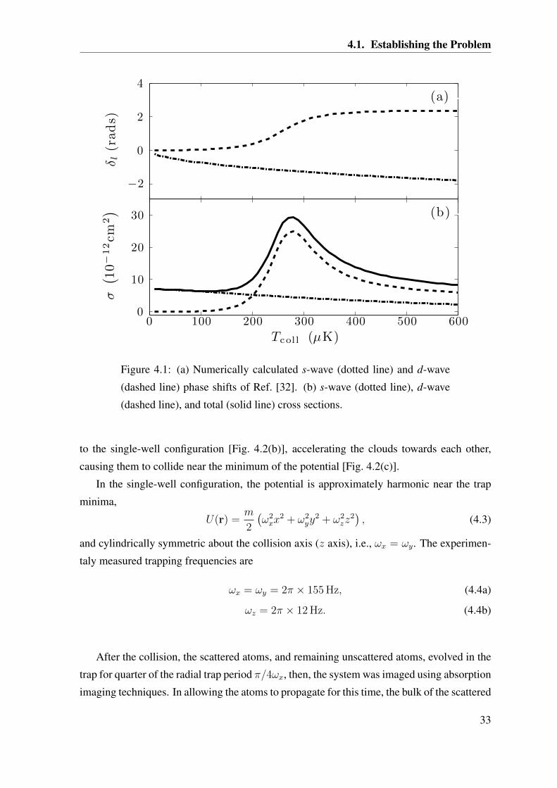
Calculation of the collision energy dependence of the phase shifts δ0 and δ2 is a nontrivial
task. The values that we use in our simulations [Fig. 4.1(a)] are those calculated by Thomas
et al. and reported in Ref. [32]. Over the range of collision energies shown in Fig. 4.1, the
interference between s- and d-wave scatterings can be important, and a d-wave resonance
also occurs. The d-wave resonance can be seen in Fig. 4.1(b) as the peak of the total cross
section, attributed to the large d-wave cross section.
4.1.2 Potential and Initial Conditions
Here, we discuss an ab initio description of the system and find such a description not pos-
sible due to the magnetic fields being insufficiently characterized. Hence, we resort to a
simplified description, which we discuss in the last portion of this section.
Ab initio model of the collider
The collisions of the clouds were performed as follows: the atoms were magnetically trapped
in a single-well configuration (quadrupole-Ioffe-configuration trap) [63], then, the trap was
adiabatically transformed into a double-well configuration [64] [Fig. 4.2(a)]. This spatially
separates two segments of the initial cloud, and the separation distance is a controllable
parameter, on which, Tcoll depends. The collision is initiated by rapidly transforming back
32
4.1. Establishing the Problem
δ l(r
ads)
−2
0
2
4
Tcoll (µK)
σ( 1
0−
12cm
2)
0 100 200 300 400 500 6000
10
20
30
(a)
(b)
Figure 4.1: (a) Numerically calculated s-wave (dotted line) and d-wave
(dashed line) phase shifts of Ref. [32]. (b) s-wave (dotted line), d-wave
(dashed line), and total (solid line) cross sections.
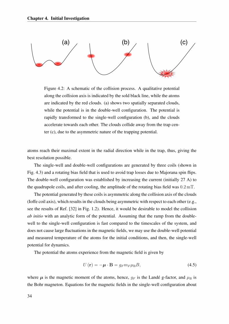
to the single-well configuration [Fig. 4.2(b)], accelerating the clouds towards each other,
causing them to collide near the minimum of the potential [Fig. 4.2(c)].
In the single-well configuration, the potential is approximately harmonic near the trap
minima,
U(r) =m
2
(ω2xx
2 + ω2yy
2 + ω2zz
2), (4.3)
and cylindrically symmetric about the collision axis (z axis), i.e., ωx = ωy. The experimen-
taly measured trapping frequencies are
ωx = ωy = 2π × 155 Hz, (4.4a)
ωz = 2π × 12 Hz. (4.4b)
After the collision, the scattered atoms, and remaining unscattered atoms, evolved in the
trap for quarter of the radial trap period π/4ωx, then, the system was imaged using absorption
imaging techniques. In allowing the atoms to propagate for this time, the bulk of the scattered
33
Chapter 4. Initial Investigation
(a) (b) (c)
Figure 4.2: A schematic of the collision process. A qualitative potential
along the collision axis is indicated by the sold black line, while the atoms
are indicated by the red clouds. (a) shows two spatially separated clouds,
while the potential is in the double-well configuration. The potential is
rapidly transformed to the single-well configuration (b), and the clouds
accelerate towards each other. The clouds collide away from the trap cen-
ter (c), due to the asymmetric nature of the trapping potential.
atoms reach their maximal extent in the radial direction while in the trap, thus, giving the
best resolution possible.
The single-well and double-well configurations are generated by three coils (shown in
Fig. 4.3) and a rotating bias field that is used to avoid trap losses due to Majorana spin flips.
The double-well configuration was established by increasing the current (initially 27 A) to
the quadrupole coils, and after cooling, the amplitude of the rotating bias field was 0.2 mT.
The potential generated by these coils is asymmetric along the collision axis of the clouds
(Ioffe coil axis), which results in the clouds being asymmetric with respect to each other (e.g.,
see the results of Ref. [32] in Fig. 1.2). Hence, it would be desirable to model the collision
ab initio with an analytic form of the potential. Assuming that the ramp from the double-
well to the single-well configuration is fast compared to the timescales of the system, and
does not cause large fluctuations in the magnetic fields, we may use the double-well potential
and measured temperature of the atoms for the initial conditions, and then, the single-well
potential for dynamics.
The potential the atoms experience from the magnetic field is given by
U (r) = −µ ·B = gFmFµBB, (4.5)
where µ is the magnetic moment of the atoms, hence, gF is the Landé g-factor, and µB is
the Bohr magneton. Equations for the magnetic fields in the single-well configuration about
34
4.1. Establishing the Problem
Mark II Ioffe-Pritchard trap 54
PSfrag replacements
z (mm)
y(mm)
AA
BB CC
100 80 60 40 20 0 -20 -40 -60
-60
-40
-20
0
20
40
60
Figure 5.9: Layout of turns and formers for the Mark II Ioffe-Pritchard trap, where the drawing isa cross-section in the plane including the symmetry axes of all the coils. Each coil is wound arounda former (light grey) with the current direction for each turn either into or out of the page (× and• respectively). A metal band (medium grey) is used to help cool the outer parts of the coils. Thequadrupole coils also have internal structure (dark grey) to ensure good water circulation in thedirections marked (large × and •). The outline extending from the right is the connection to thevacuum system and glass cell. The position of the MOT (∗) and magnetic trap (#) are shown withlarge markers, and the position (z, y) = (0,0) corresponds to the previous position of the MOT. Theprobe laser beam travels perpendicularly out of the page.
Quadrupole Coil A
Quadrupole Coil B
Ioffe Coil(s)
XX
X
z
y
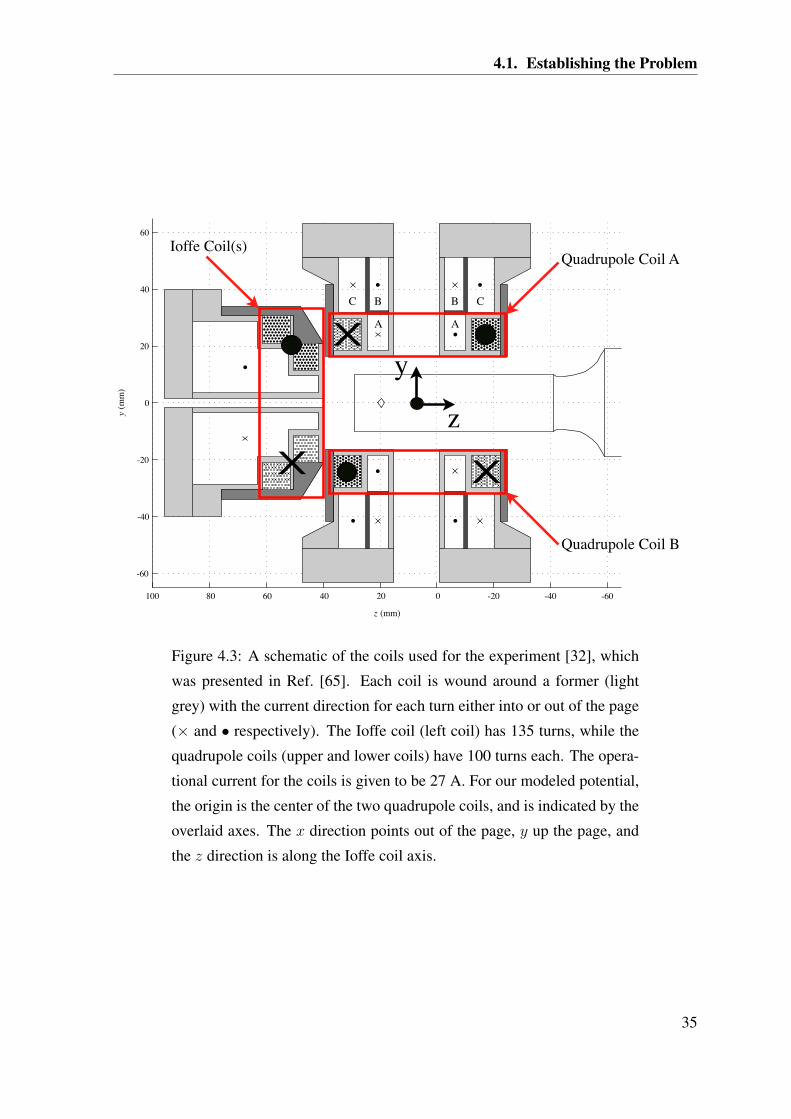
Figure 4.3: A schematic of the coils used for the experiment [32], which
was presented in Ref. [65]. Each coil is wound around a former (light
grey) with the current direction for each turn either into or out of the page
(× and • respectively). The Ioffe coil (left coil) has 135 turns, while the
quadrupole coils (upper and lower coils) have 100 turns each. The opera-
tional current for the coils is given to be 27 A. For our modeled potential,
the origin is the center of the two quadrupole coils, and is indicated by the
overlaid axes. The x direction points out of the page, y up the page, and
the z direction is along the Ioffe coil axis.
35
Chapter 4. Initial Investigation
the trap center are given in Ref. [65]. However, we require analytic equations that extend
over the entire range that the atoms occupy during the course of the collision, for the initial
conditions, as well as, implementing the collisionless evolution of the test particles in the
DSMC algorithm [Eqs. (3.4a)−(3.4c)]. To do this, we extend the methods of Ref. [65],
by treating the coils in Fig. 4.3 as current densities, and using the Biot-Savart law. This
requires an expansion about the center of the quadrupole coils (see Fig. 4.3), and the resulting
magnetic field magnitude must be time averaged, since the total magnetic field includes the
rotating bias field. The potential is well approximated by a harmonic potential in the x and
y dimensions, however, along the collision axis (z axis), the potential is asymmetric and
requires z terms to be kept to tenth order. This causes the clouds to collide away from
the single-well minima, and have different velocities. Furthermore, the harmonic trapping
frequencies in the x and y directions vary along the collision axis, which leads to the clouds
having different initial shapes and undergoing different shape oscillations as they accelerate
towards the trap center.
About the single-well minima, the trapping frequencies determined by our model are
ωx = ωy = 2π × 122 Hz, (4.6a)
ωz = 2π × 15 Hz, (4.6b)
which is a different from the experimentally measured frequencies Eqs. (4.4). Thus, the mod-
eled potential is not sufficiently accurate for a quantitative ab initio comparison.1 However,
we qualitatively observe the dynamics of the experimental setup.
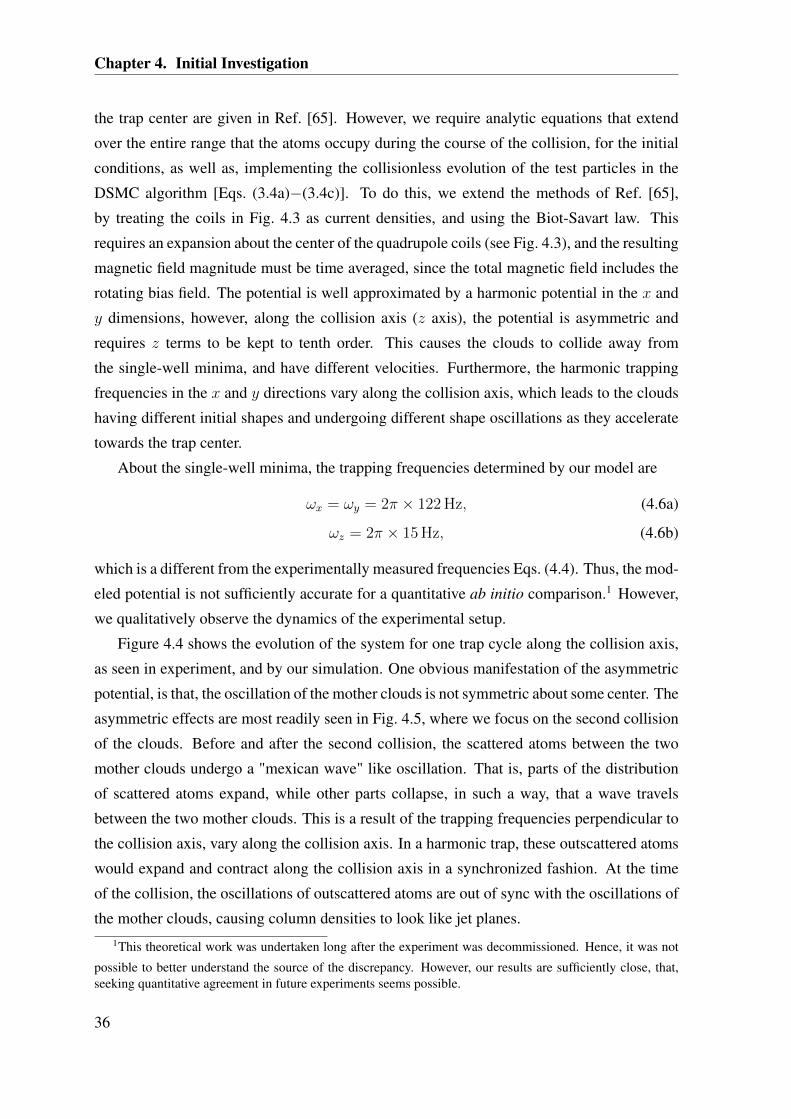
Figure 4.4 shows the evolution of the system for one trap cycle along the collision axis,
as seen in experiment, and by our simulation. One obvious manifestation of the asymmetric
potential, is that, the oscillation of the mother clouds is not symmetric about some center. The
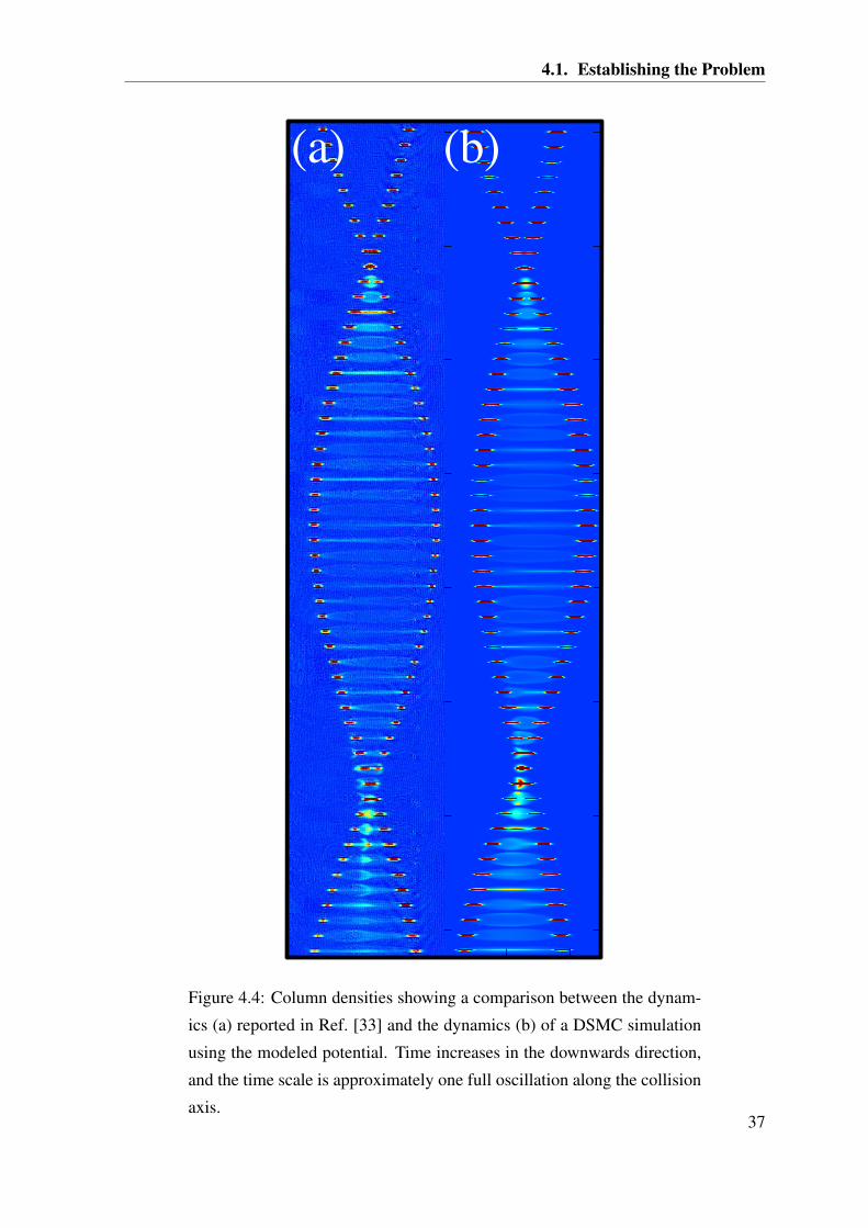
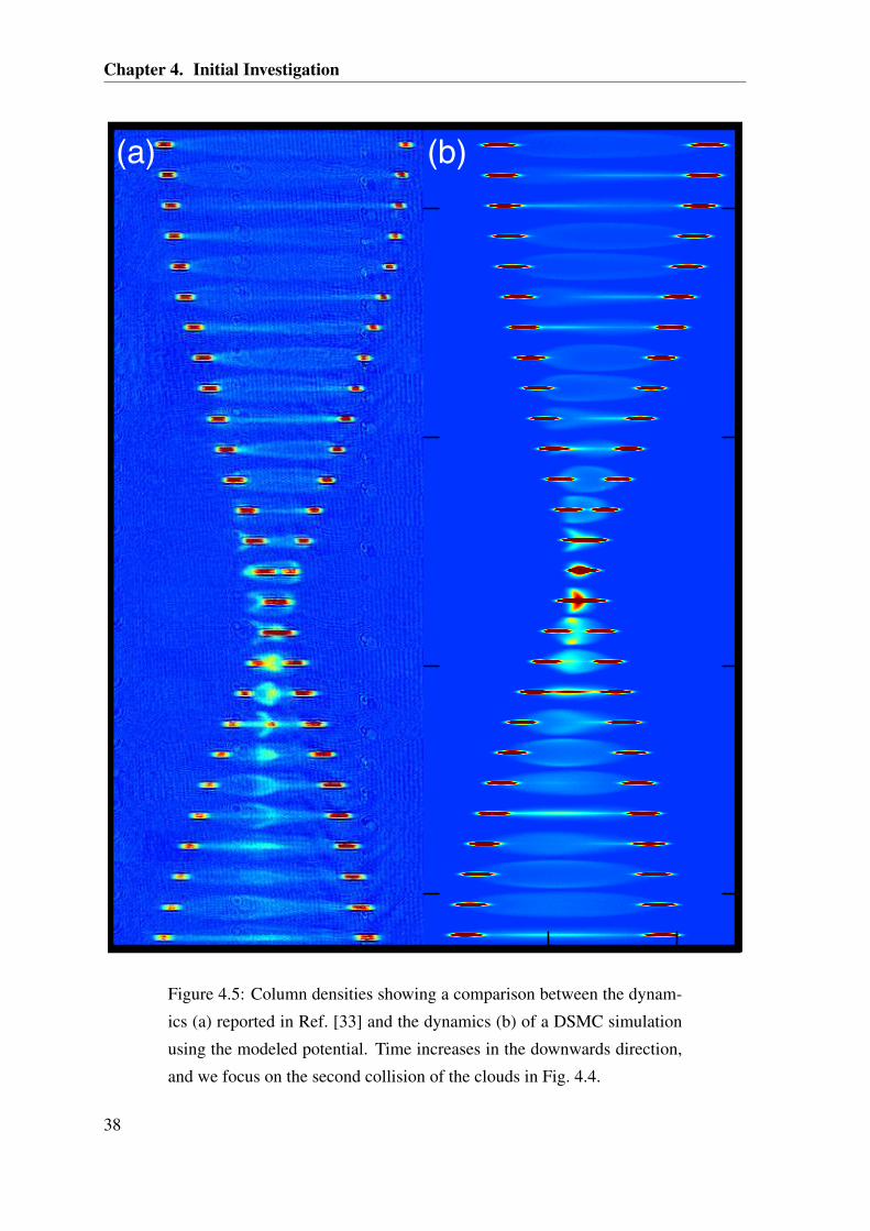
asymmetric effects are most readily seen in Fig. 4.5, where we focus on the second collision
of the clouds. Before and after the second collision, the scattered atoms between the two
mother clouds undergo a "mexican wave" like oscillation. That is, parts of the distribution
of scattered atoms expand, while other parts collapse, in such a way, that a wave travels
between the two mother clouds. This is a result of the trapping frequencies perpendicular to
the collision axis, vary along the collision axis. In a harmonic trap, these outscattered atoms
would expand and contract along the collision axis in a synchronized fashion. At the time
of the collision, the oscillations of outscattered atoms are out of sync with the oscillations of
the mother clouds, causing column densities to look like jet planes.1This theoretical work was undertaken long after the experiment was decommissioned. Hence, it was not
possible to better understand the source of the discrepancy. However, our results are sufficiently close, that,seeking quantitative agreement in future experiments seems possible.
36
4.1. Establishing the Problem
200 400
2000
4000
6000
8000
10000
12000
14000
16000
Obtaining scattering pattern images 93
3 ms
69 ms!
Figure 6.4: The dynamics of the two clouds after the ramp to the single-well trap
is initiated. The images are taken at times between tdelay = 3 ms and tdelay = 69 ms
in steps of 1 ms. The clouds first collide at tdelay ≈ 24 ms and a second collision
occurs at tdelay ≈ 58 ms.
(a) (b)
Figure 4.4: Column densities showing a comparison between the dynam-
ics (a) reported in Ref. [33] and the dynamics (b) of a DSMC simulation
using the modeled potential. Time increases in the downwards direction,
and the time scale is approximately one full oscillation along the collision
axis.37
Chapter 4. Initial Investigation
200 400
2000
4000
6000
8000
10000
12000
14000
16000
Obtaining scattering pattern images 93
3 ms
69 ms!
Figure 6.4: The dynamics of the two clouds after the ramp to the single-well trap
is initiated. The images are taken at times between tdelay = 3 ms and tdelay = 69 ms
in steps of 1 ms. The clouds first collide at tdelay ≈ 24 ms and a second collision
occurs at tdelay ≈ 58 ms.
(a) (b)
(a) (b)
Figure 4.5: Column densities showing a comparison between the dynam-
ics (a) reported in Ref. [33] and the dynamics (b) of a DSMC simulation
using the modeled potential. Time increases in the downwards direction,
and we focus on the second collision of the clouds in Fig. 4.4.
38
4.1. Establishing the Problem
Simplified potential and initial conditions
Being restricted by the lack of a quantitative description of the potential, the problem is sim-
plified by taking the potential to be the harmonic form given in Eq. (4.3) with the measured
trapping frequencies Eqs. (4.4).
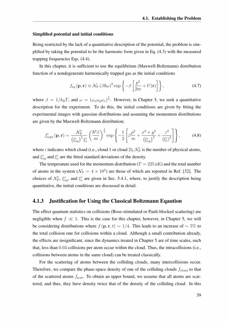
In this chapter, it is sufficient to use the equilibrium (Maxwell-Boltzmann) distribution
function of a nondegenerate harmonically trapped gas as the initial conditions
feq (p, r) ≡ NP (β~ω)3 exp
−β[p2
2m+ U(r)
], (4.7)
where β = 1/kBT , and ω = (ωxωyωz)13 . However, in Chapter 5, we seek a quantitative
description for the experiment. To do this, the initial conditions are given by fitting the
experimental images with gaussian distributions and assuming the momentum distributions
are given by the Maxwell-Boltzmann distribution;
f iexpt (p, r) =N i
P(ξixy)2ξiz
(~2β
m
) 32
exp
−1
2
[βp2
m+x2 + y2
(ξixy)2 +
z2
(ξiz)2
], (4.8)
where i indicates which cloud (i.e., cloud 1 or cloud 2),N iP is the number of physical atoms,
and ξixy and ξiz are the fitted standard deviations of the density.
The temperature used for the momentum distribution (T = 225 nK) and the total number
of atoms in the system (NP = 4 × 10⁵) are those of which are reported in Ref. [32]. The
choices of N iP, ξixy, and ξiz are given in Sec. 5.4.1, where, to justify the description being
quantitative, the initial conditions are discussed in detail.
4.1.3 Justification for Using the Classical Boltzmann Eqaution
The effect quantum statistics on collisions (Bose-stimulated or Pauli-blocked scattering) are
negligible when f 1. This is the case for this chapter, however, in Chapter 5, we will
be considering distributions where f (p, r, t) ∼ 1/4. This leads to an increase of ∼ 5% to
the total collision rate for collisions within a cloud. Although a small contribution already,
the effects are insignificant, since the dynamics treated in Chapter 5 are of time scales, such
that, less than 0.03 collisions per atom occur within the cloud. Thus, the intracollisions (i.e.,
collisions between atoms in the same cloud) can be treated classically.
For the scattering of atoms between the colliding clouds, many intercollisions occur.
Therefore, we compare the phase-space density of one of the colliding clouds fcloud to that
of the scattered atoms fscat. To obtain an upper bound, we assume that all atoms are scat-
tered, and thus, they have density twice that of the density of the colliding cloud. In this
39

Chapter 4. Initial Investigation
case, fcloud/fscat ≈ 2∆Pscat/∆Pcloud, where ∆Pcloud and ∆Pscat are the momentum-space
volumes which the cloud and the scattered atoms occupy, respectively. Figure 4.6 shows a
qualitative depiction of the initial clouds and scattered atoms: the momentum widths of the
cloud can be approximated by h/λth, where λth is the thermal de Broglie wavelength. The
momentum-space volume of the scattered atoms can be approximated by πp2collh/λth, where
p2coll = 4mkBTcoll is the relative momentum of the clouds (πp2
coll is the surface area of the
collision sphere). Thus, in terms of temperatures, f iexpt/fscat = 4Tcoll/T . For the collisions
we consider here, Tcoll ≈ 1000T , giving fscat to be three orders of magnitude smaller than
f iexpt, hence, the intercollisions can also be treated classically.
py
pz
pcoll
hλth
Figure 4.6: A qualitative depiction of the initial clouds (blue) and the
scattered atoms (red) in the (py, pz) plane.
4.2 Tests and Optimal Parameters for DSMC
In this section, we develop tests relevant to ultracold systems that we use to validate and to
explore how to optimize the performance of the DSMC algorithm by quantifying the effects
of the adaptive enhancements. Primarily, we are interested in the quality of the represen-
40

4.2. Tests and Optimal Parameters for DSMC
tation of the phase-space distribution, since this is of fundamental importance for accurate
Boltzmann evolution. In particular, we address the effects of increasing the number of test
particles, and refining the grid, on collision rates as compared to exact results.
4.2.1 Analytic Results
We develop benchmark analytic results to calibrate the algorithm against. To do this we con-
sider the equilibrium (Maxwell-Boltzmann) distribution function for a harmonically trapped
gas Eq. (4.7).
The total collision rate is given by
R =σ0
m
∫d3p
h3
∫d3p1
h3
∫d3r |p1 − p| ff1. (4.9)
Here, we have taken the differential cross section to be velocity independent to give a total
cross section of σ0. Evaluating this expression for the equilibrium cloud, Eq. (4.7), we obtain
Req =N 2
P
2π2mβω3σ0. (4.10)
As we are concerned with simulating the collisions of equilibrium clouds, it will be useful
to consider the instantaneous distribution,
fcoll (p, r) = feq (p + p0z, r) + feq (p− p0z, r) , (4.11)
which corresponds to two spatially overlapping clouds with equilibrium shapes that are trav-
eling with opposite momenta ±p0 along the z direction. The total collision rate for this case
is
Rcoll =N 2
P
2π2mβω3σ0
[2 + exp
(−p2
0
β
m
)
+1
2p0
√πm
β
(1 + 2p2
0
β
m
)erf
(p0
√β
m
)]. (4.12)
For small p0, the term in the square brackets scales as 4 + 23βp2
0/m + O (p40), showing that,
for p0 = 0, Eq. (4.12) reduces to Eq. (4.10) with NP → 2NP, as expected. While for large
p0, it scales as 2 +√βπ/mp0 + O
(p−1
0
). The first term corresponds to the intra cloud
collisions, while the linear term is obtained for the case of Dirac delta-function momentum
distributions, δ (p± p0z).
41

Chapter 4. Initial Investigation
4.2.2 Grid Parameters and Test Particle Number
To investigate the accuracy with which collisions are treated, we compare the numerical
collision rate to the exact values in Eqs. (4.10) and (4.12). To do this, we calculate the
relative error of the numerical collision rate and examine its dependence on the number of
test particles and grid refinement.2
Numerical Collision Rate
For the purpose of comparison, we need to extract a collision rate from the DSMC represen-
tation of f (p, r, t). To do this, we evaluate the mean number of collisions in each cell over
some time δtc. Hence, in each cell, the mean collision rate per unit volume is
Rc ≈ 2αMc∑
(ij)
Pij∆Vcδtc
, (4.13)
where (ij) indicates the indices of the Mc selected collision pairs in the cell. Thus, the total
collision rate for the system is
R =∑
cells
Rc∆Vc. (4.14)
By calculating the collision rate in this way, we are, in effect, directly performing a Monte
Carlo integration for the integral (4.9), which is the basis of the derivation of the collision
probability in Ref. [18] (also see Sec. 6.1). The time step for the cell δtc is somewhat arbi-
trary, and we choose it to give Mc = bNc/2c collision pairs.
A convenient length scale for the trapped system is given by the thermal widths
Wi =√
2kBT/mω2i , (4.15)
for the ith dimension, and we choose the master cell widths such that the resolution in each
direction (relative to these widths) are the same, i.e.,
γ =∆x
Wx
=∆y
Wy
=∆z
Wz
. (4.16)
In what follows, γ will serve as an important parameter to specify the fineness of the spatial
resolution.
2The relative error in the collision rate is independent of NP and σ0.
42
4.2. Tests and Optimal Parameters for DSMC
Accuracy
To increase the accuracy of our numerical calculation of the total collision rate, we must
improve the accuracy of our representation of continuous distribution f (p, r, t) or take more
samples. In the DSMC algorithm, f (p, r, t) is represented in two ways: (i) the test-particle
swarm, (ii) the grid of cells that sample the test-particle swarm. In Sec. 3.3.3, the discussion
for the number of tested collisions shows that, without cell adaption [i.e., LACs or LATSs],
(i) and (ii) are largely decoupled. However, simply decreasing the size of the master cells
can cause large statistical fluctuations in the number of collisions, as single occupation of a
cell becomes more common, hence, requiring a larger number of samples.
Our LAC scheme essentially establishes a local maximum size of the cells (i.e., maxi-
mum error), which is set byNT, Nth, and n (r, t). In our results, this is seen for the collision
rate of the equilibrium cloud given in Fig. 4.7. These results show that the magnitude of the
relative error does not continue to increase with increasing γ (as it does in the unadapted
case), but tends to a constant dependent on Nth. With decreasing Nth, smaller cell sizes
are achieved, hence, lower error.3 However, we restrict ourselves to Nth ≥ 2 to avoid the
increasingly large statistical fluctuations mentioned earlier. The results in Fig. 4.7 remain
qualitatively similar for different values of NT, however, the fluctuations (i.e., error bars
Fig. 4.7) increase with decreasing test-particle number.
It is worth noting that systems with identical density distributions are coarse grained
in the same fashion (provided NT is the same when using the LAC scheme), hence, they
have the same accuracy. For example, the equilibrium (4.7) and collision (4.11) distributions
have identical relative error profiles as seen in Fig. 4.7. However, if a system is dynami-
cally changing and no adaption was employed, evolving to a more dilute system would de-
crease the magnitude of the relative error, while increasing if becoming denser. For adaptive
schemes, this is not an issue, as the cell sizes automatically adjust to this change.
Performance Considerations
The results in Fig. 4.7 show that the following cases approximately have the same relative
error in collision rate:
(i) SIM1: An unadaptive simulation with γ = 0.02.
3Care needs to be taken with other adaptive schemes, since the approach outlined in Sec. 3.3.3, to remove
statistical biasing, neglects to take into account statistical fluctuations from other sources (e.g., cell volume),
which may become important [66].
43
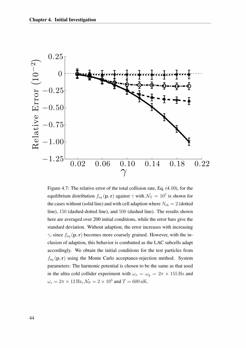
Chapter 4. Initial Investigation
Rela
tive
Err
or( 1
0−
2)
γ0.02 0.06 0.10 0.14 0.18 0.22
−1.25
−1.00
−0.75
−0.50
−0.25
0
0.25
Figure 4.7: The relative error of the total collision rate, Eq. (4.10), for the
equilibrium distribution feq (p, r) against γ with NT = 107 is shown for
the cases without (solid line) and with cell adaption whereNth = 2 (dotted
line), 150 (dashed-dotted line), and 500 (dashed line). The results shown
here are averaged over 200 initial conditions, while the error bars give the
standard deviation. Without adaption, the error increases with increasing
γ, since feq (p, r) becomes more coarsely grained. However, with the in-
clusion of adaption, this behavior is combatted as the LAC subcells adapt
accordingly. We obtain the initial conditions for the test particles from
feq (p, r) using the Monte Carlo acceptance-rejection method. System
parameters: The harmonic potential is chosen to be the same as that used
in the ultra cold collider experiment with ωx = ωy = 2π × 155 Hz and
ωz = 2π × 12 Hz, NP = 2× 10⁵ and T = 600 nK.
44

4.2. Tests and Optimal Parameters for DSMC
(ii) SIM2: A LAC simulation with Nth = 2 and γ = 0.2, which we also include LATSs
for dynamics.
A fuller picture of the merits of using either of these approaches for a simulation requires us
to understand their resource requirements.
Speed: We find that, with our code SIM2 is approximately five times faster than SIM1 for
near-equilibrium evolution. Note, we only use the LATS scheme in SIM2 for the master
cells (as discussed at the end of Sec. 3.3.4). It should also be noted that this performance
indicator is dependent on the code implementation and physical problem under consideration
(i.e., equilibrium cloud versus highly nonequilibrium situation).
Storage: SIM1 requires ∼ 5× 10⁷ master cells, while SIM2 requires∼ 5× 10⁴ master cells
with a maximum of 4096 LAC subcells within a master cell (typically requiring a total of
∼ 7× 10⁶ LAC subcells).
4.2.3 Collisions Between Clouds: Comparison to Simple Methods
In this subsection, we consider the collision of two equilibrium clouds in a harmonic trap,
feq (p± p0z, r∓ r0z), shown schematically in Fig. 4.8. We study this collision using our
DSMC algorithm and compare its results to a simplified model that has been used previously
to analyze this problem. Initially, the two clouds are centered at locations separated by
a distance of 2r0 along the z direction, chosen to ensure that (initially) the clouds do not
overlap. The clouds approach each other, moving at a relative momentum of 2p0, and when
they overlap, collisions scatter atoms out of the clouds. Here, our main interest is the total
number of such scattered atoms Nsc, after the two clouds have completed passing through
each other.
The simple model we consider was used in Ref. [32] (see also, Ref. [67]) and was derived
from the BE description of the colliding clouds by making the following approximations:
(a1) The harmonic potential is ignored (collision taken to be in free space).
(a2) The momentum distribution of each cloud is replaced by δ (p± p0z).
(a3) The dynamics of scattered atoms are neglected.
These approximations lead to equations for the densities ni (r, t) of cloud i = a, b,(∂
∂t± vr
2
∂
∂z
)ni (r, t) = −vrσ0na (r, t)nb (r, t) , (4.17)
where vr = 2p0/m. We can solve these equations directly using a pseudo-spectral method.
45

Chapter 4. Initial Investigation
2r0
cloud 1 cloud 2p0
-p0
Figure 4.8: A schematic of the ultra-cold-atom collider used in Sec. 4.3.
Two clouds initially separated by a distance of 2r0 collide at a relative
momentum of 2p0. The number of atoms that have scattered out of the
clouds, after they have passed through each other, is referred to as Nsc.
An analytic expression may be derived with an additional approximation:
(a4) The loss of atoms is small enough such that the shape of the densities do
not deform but remain Gaussian while the normalization of each cloudNP
decreases.
Using this, one can integrate Eq. (4.17) over all position space to find the total number of
scattered atoms from the collision,
Nsc =N 2
P
4πmβωxωyσ0. (4.18)
As shown in Sec. 4.2.1, when considering the limiting behavior of Eq. (4.12), the approx-
imation (a2) is satisfied when Tcoll T (which is the case for collider velocities we consider
here). That the momentum distributions can be replaced with Dirac δ functions is consistent
with the quantum statistics not playing a significant role in the scattering that occurs when
the two clouds collide. However, the internal motion of each cloud can be influenced by
quantum statistics.
As the full DSMC solution includes the dynamics of scattered atoms, it is useful to split
the scattered atoms into two groups: (i) scattered atoms that have not undergone any sub-
sequent collisions, (ii) scattered atoms that have undergone additional collisions, including
all collision partners.4 All of the scattered atoms predicted by Eqs. (4.17) and (4.18) are of
group (i).
In Eqs. (4.17) and (4.18),Nsc is independent of the details of the differential cross section
(only depending on the total cross section), and this is largely true for the full solution in the
4We include atoms that are scattered out of cloud 1 or 2 by a collision with an already scattered atom.
46
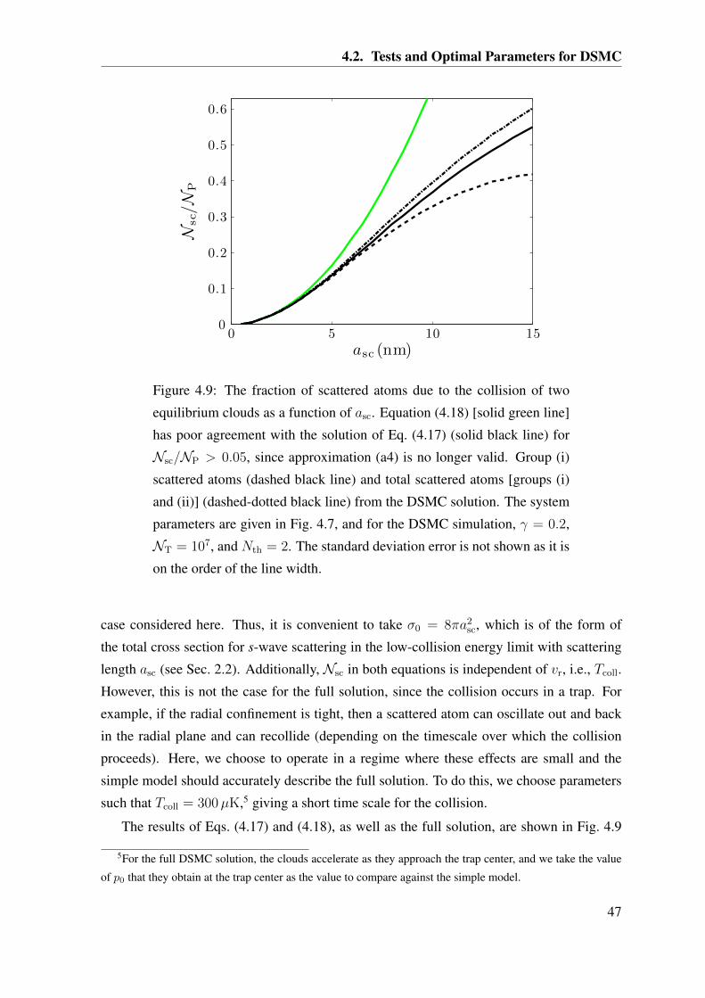
4.2. Tests and Optimal Parameters for DSMC
Nsc/N
P
asc (nm)0 5 10 15
0
0.1
0.2
0.3
0.4
0.5
0.6
Figure 4.9: The fraction of scattered atoms due to the collision of two
equilibrium clouds as a function of asc. Equation (4.18) [solid green line]
has poor agreement with the solution of Eq. (4.17) (solid black line) for
Nsc/NP > 0.05, since approximation (a4) is no longer valid. Group (i)
scattered atoms (dashed black line) and total scattered atoms [groups (i)
and (ii)] (dashed-dotted black line) from the DSMC solution. The system
parameters are given in Fig. 4.7, and for the DSMC simulation, γ = 0.2,
NT = 107, and Nth = 2. The standard deviation error is not shown as it is
on the order of the line width.
case considered here. Thus, it is convenient to take σ0 = 8πa2sc, which is of the form of
the total cross section for s-wave scattering in the low-collision energy limit with scattering
length asc (see Sec. 2.2). Additionally, Nsc in both equations is independent of vr, i.e., Tcoll.
However, this is not the case for the full solution, since the collision occurs in a trap. For
example, if the radial confinement is tight, then a scattered atom can oscillate out and back
in the radial plane and can recollide (depending on the timescale over which the collision
proceeds). Here, we choose to operate in a regime where these effects are small and the
simple model should accurately describe the full solution. To do this, we choose parameters
such that Tcoll = 300µK,5 giving a short time scale for the collision.
The results of Eqs. (4.17) and (4.18), as well as the full solution, are shown in Fig. 4.9
5For the full DSMC solution, the clouds accelerate as they approach the trap center, and we take the value
of p0 that they obtain at the trap center as the value to compare against the simple model.
47
Chapter 4. Initial Investigation
for varying asc. All models agree well in the low scattering regime Nsc/NP < 0.05, while
for higher scattering fractions, approximation (a4) becomes invalid, and the dynamics of the
scattered atoms becomes increasingly important. However, the solution of Eq. (4.17) agrees
to within 10% of the relative error to the total [groups (i) and (ii) combined] scattered fraction
given by the full solution over the whole range.
We can modify the collision problem and DSMC method to a regime that is exactly
described by the simplified equation (4.17). To do this, all particles are taken to have mo-
mentum ±p0 along the z axis (the components of momenta in the xy plane are zero) and
evolve without an external trapping potential. Consistent with the approximations going into
Eq. (4.17), whenever a pair of particles undergoes a collision, it is removed from the sys-
tem (eliminating any need for consideration of multiple collisions). Due to the form of the
distribution function, NNCs cannot be used.6
The relative error ofNsc as calculated by the DSMC solution to that of our numerical so-
lution of Eq. (4.17) is shown in Fig. 4.10 for the two casesNT = 105 and 107. The excellent
agreement of the two results is a good test that the DSMC method is correctly implemented.
The error bars represent the statistical fluctuations of the DSMC results. These fluctuations
reduce with increasing asc asNsc increases, while between the two cases, they are reduced by
a factor of 10, since they also decrease with increasing NT (to be definite, these fluctuations
are given by the inverse square root of the number of scattered test particles).
6Particles have no transverse momenta, thus particles from the same cloud never leave the proximity of each
other. Hence, it is required that a particle from one cloud is closest to a particle from the other cloud before a
collision can occur, which results in a decreased number of collisions.
48

4.2. Tests and Optimal Parameters for DSMC
Rel
ati
ve
Err
or
asc (nm)0 5 10 15
−.10
−0.05
0
0.05
0.10
Figure 4.10: The relative error ofNsc as calculated by the DSMC solution
of Eq. (4.17) [see text] to that of our pseudo spectral solution of Eq. (4.17).
Here, we show the two cases NT = 105 (black) and 107 [green] with
γ = 0.2, Nth = 25, and the system parameters given in Fig. 4.7. We use
ηcoll = ηtr = 0.01, and ηmax = 0.1. The results shown here are averaged
over 200 simulations, while the error bars give the standard deviation.
49

Chapter 4. Initial Investigation
4.3 Many-body simulation of an ultra-cold-atom collider
In this section, we demonstrate the application of our DSMC algorithm to the simulation
of the ultra-cold-atom collider reported in Ref. [32]. The main extension, over the DSMC
collision test presented in Sec. 4.2.3, is the inclusion of the full two-body collisional cross
section needed for a realistic microscopic description of the collisional interactions. We
then extend our consideration to the long-time dynamics of the collider and how the system
progresses to equilibrium.
4.3.1 DSMC simulations
Using the full energy and angular-dependent-scattering cross section, we present the results
of column densities calculated after two equilibrium clouds feq (p± p0z, r∓ r0z) have col-
lided for the cases Tcoll = 200µK and 300µK. Following the experimental procedure [32],
we calculate these column densities at a quarter of the radial trap period (π/2ωx) after the
clouds reach the center of the trap. At this time the bulk of the scattered atoms reach their
maximal extent in the radial direction. Figures 4.11(a) and 4.11(c) show a regime of s- and
d-wave interference (Tcoll = 200µK), while Figs. 4.11(b) and 4.11(d) show a d-wave regime
(Tcoll = 300µK). Clearly, the distribution of scattered atoms deviates from the typical s-
wave halo (e.g., see Ref. [68]).
4.3.2 Long-time dynamics: Rethermalization
The idea of using rethermalization of colliding condensates to perform calorimetry has been
proposed in Ref. [69], however, no direct simulations were made of the thermalization dy-
namics. More generally, there has been significant recent interest in how a quantum system
rethermalizes [70], particularly in systems that might be experimentally realized with ultra-
cold-atomic gases (e.g., see Refs. [71, 72]). To date, much of the attention has focused on
integrable or nearly integrable systems where numerical solutions are available for small
samples of atoms (typically NP < 102). However, in such regimes, thermalization is often
inhibited or is strongly affected by constraints (e.g., see Ref. [73]) as well as being difficult to
explore experimentally due to the small atom number (or requiring many similarly prepared
systems to get a good signal).
Thus, we are motivated to apply the DSMC method to model the dynamics of colliding
ultracold clouds well past the first collision. As the collisions occur in the trap, the clouds will
oscillate back and forth, recolliding each time, and thus, are provided with the opportunity
50

4.3. Many-body simulation of an ultra-cold-atom collider
−250
0
250
y(µ
m)
−500 0 500−250
0
250
z (µm)
−500 0 500
0 0.3 0.6 0.9 1.2 1.5 1.8(µm−2
)
(a) (b)
(c) (d)
200 µK 300 µK
Figure 4.11: Column densities at time π/2ωx after the clouds reach the
center of the trap. Tcoll = 200µK [(a) and (c)] is a regime of s- and d-
wave interference, while Tcoll = 300µK [(b) and (d)] is a d-wave regime.
(c) and (d) only show the scattered atoms. The initial conditions for the
clouds are chosen as in Sec. 4.2.3, and the system parameters are given
in Fig. 4.7, while the simulation parameters are γ = 0.2, NT = 105,
and Nth = 2. The results were averaged over 200 simulations. Note, we
have compared these results to simulations with NT = 107 also averaged
over 200 runs, and we find that the number of scattered particles and the
angular scattering distributions agreed to within 1%.
51
Chapter 4. Initial Investigation
to rethermalize. This system is much larger and classical in nature than the small quantum
systems generically considered for thermalization studies. However, we believe this is an in-
teresting system: first as a bridge between quantum and classical thermalization in ultracold
gases that is practical for experimental investigation. Second, such a system might provide a
unique opportunity to test the BE in a regime where the microscopic parameters are precisely
known and with well-characterized far-from-equilibrium initial conditions. Few equations in
theoretical physics have evoked as much discussion and controversy as the BE – particularly
in reference to the introduction of irreversibility – and such a test could be of broad interest
and shed light on some long-standing issues in statistical mechanics.
Our first evidence for thermalization comes from examining the density profiles of the
colliding clouds at times after the first collision. Some examples of these density profiles
are shown in Figs. 4.12(a)-4.12(d) and reveal that, as time passes, the number of atoms
participating in the parametric oscillation of the mother clouds along the z axis decreases as
the collisions convert the system to a more isotropic form. Indeed, the system clearly appears
to increase entropy and approaches an equilibrium like configuration.
In order to quantify the approach to equilibrium, it is useful to consider how various
moments of the system evolve dynamically. In Fig. 4.13, we show the envelope of the os-
cillations in the position spread moment 〈r2〉1/2 = 〈x2 + y2 + z2〉1/2, characterizing the
root-mean square of the distance of the particles from the trap center. [Note the oscillations
of this moment occur on a much faster timescale and are shown in an inset to Fig. 4.13.]
These results show that the system rethermalizes quite rapidly over the first approximately
five trap periods. The number of collisions per particle over the first approximately three trap
periods is shown in the inset to Fig. 4.13. The steps in collision number, which are initially
apparent, arise from the periodic recolliding of the clouds. However, as the system is dis-
tributed over modes, these steps smooth out. These results show that, during this initial rapid
phase of rethermalization, atoms experience & 10 collisions, much greater than the value of
2.7 often quoted in the literature from the study of Wu and Foot [13].
After this rapid thermalization phase, the relaxation to equilibrium proceeds more slowly
as energy contained within a few low-frequency collective modes waits to be damped. We
find that two modes are dominant on long time scales. Most importantly, a mode that oscil-
lates at 2ωx(= 2ωy) is dominated by radial breathing character and is well described (both
frequency and damping) by the analytic predictions given in Ref. [12].7 Also, we note that
the rate of relaxation is strongly dependent on the trapping geometry and collision rate. The
analytical predictions are only applicable when the system is near the final equilibrium state,
7Calculations based on these analytic prediction were performed by Danny Baillie.
52

4.3. Many-body simulation of an ultra-cold-atom collider
−150
0
150y
(µm
)
−300 0 300−150
0
150
z (µm)
−300 0 300
0 25 50 75(µm−2
)
(a) (b)
(c) (d)
Figure 4.12: Column densities illustrating the long time dynamics of
rethermalization. (a) At time tωz = 7.04 after the clouds have passed
through each other twice. The colliding clouds are still visible (density
peaks). When the colliding clouds are depleted, the system continues to
evolve through collective oscillations that are illustrated by the images (b)
and (c) at tωz = 18.85 and 19.60, respectively. The decay of these col-
lective oscillations occurs on a slower time scale than the depletion of the
colliding clouds, and the distribution does not take on the equilibrium dis-
tribution until much later times as seen in (d) at tωz = 500.02. The trap
frequencies are ωz = 2π × 50 Hz and ωx = ωy = 2ωz, and each of the
initial clouds has NP = 106 and T = 600 nK. We use an isotropic dif-
ferential cross section with asc = 10 nm. The initial separation is chosen
such that there is insignificant overlap of the clouds. The momenta are
chosen to give Tcoll = 32.4µK, giving a final equilibrium temperature of
T = 6µK. Note, for an isotropic trap, the system does not completely
thermalize without mean-field effects, since the breathing mode does not
damp [12].
53

Chapter 4. Initial Investigation
tωz
⟨ r2⟩ 1
/2
(µm
)
100 200 300 400 500
40
60
80
100
120
⟨ r2⟩ 1
/2
(µm
)
80 90 10085
90
95
100
Col.
/ A
tom
0 10 200
5
10
Figure 4.13: Envelope of the oscillations (as seen in the lower inset) of the
root-mean-square of r. The rapid decay of the envelope within the first ten
trap cycles is attributed to the depletion of the colliding clouds, while the
slower decay is the decay of the collective modes. The upper inset shows
the mean number of collisions per atom.
as they use the Gaussian anstaz
f (p, r, t) =NP~3
ξ2xyξzζ
2xyζz
exp
[−1
2
(p2x + p2
y
ζ2xy
+p2z
ζ2z
+x2 + y2
ξ2xy
+z2
ξ2z
)], (4.19)
where the standard deviations hold the time dependence.
In relation to thermalization dynamics, it is interesting to revisit the role of test particles
in the DSMC simulation. In general, increasing NT has the effect of reducing fluctuations
in a simulation and, hence, the number of trajectories needed to obtain an ensemble average.
However, in order to gain a better understanding of typical results (and, hence, fluctuations)
that might be expected in experiments, it is necessary to take NT = NP. To illustrate this,
we show some results for a small amplitude collective-mode oscillation in Fig. 4.14 for
54
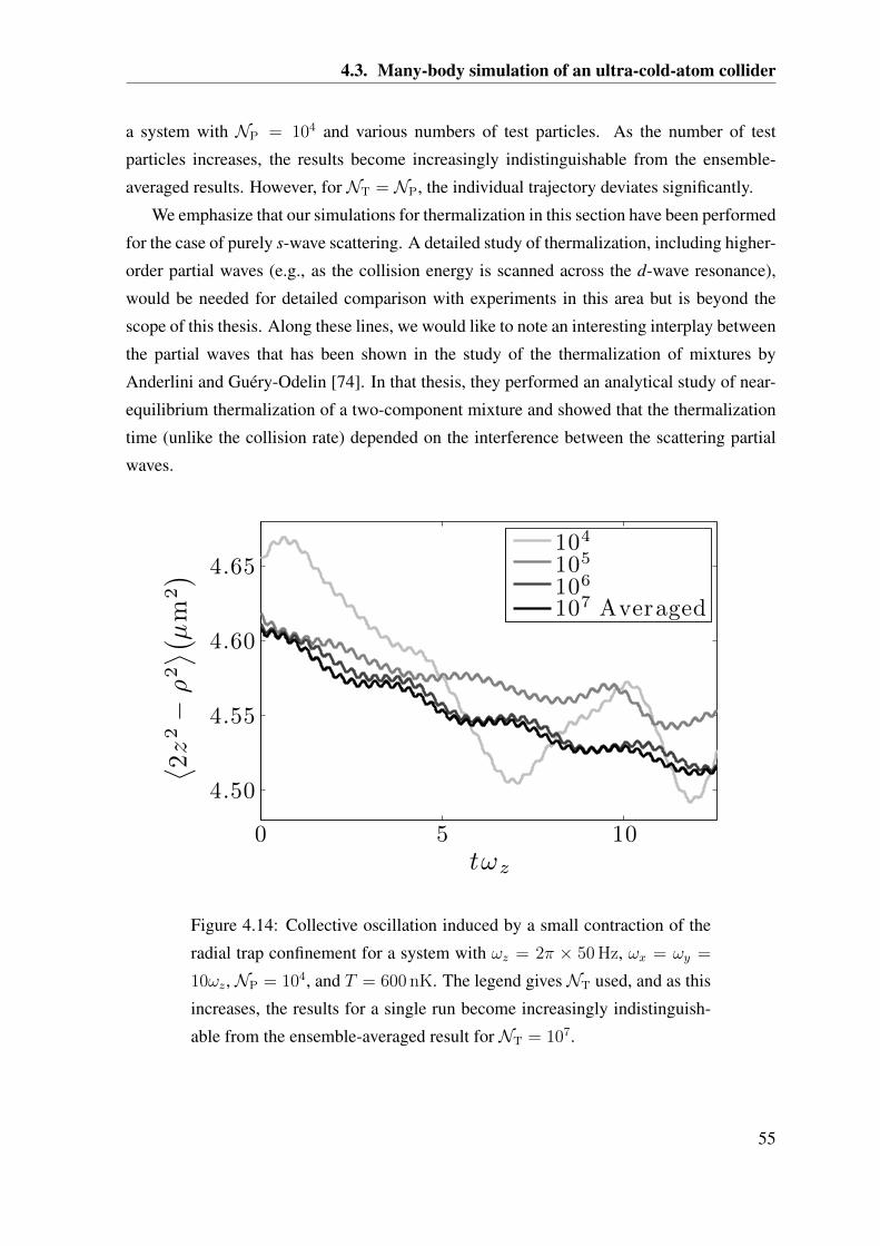
4.3. Many-body simulation of an ultra-cold-atom collider
a system with NP = 104 and various numbers of test particles. As the number of test
particles increases, the results become increasingly indistinguishable from the ensemble-
averaged results. However, for NT = NP, the individual trajectory deviates significantly.
We emphasize that our simulations for thermalization in this section have been performed
for the case of purely s-wave scattering. A detailed study of thermalization, including higher-
order partial waves (e.g., as the collision energy is scanned across the d-wave resonance),
would be needed for detailed comparison with experiments in this area but is beyond the
scope of this thesis. Along these lines, we would like to note an interesting interplay between
the partial waves that has been shown in the study of the thermalization of mixtures by
Anderlini and Guéry-Odelin [74]. In that thesis, they performed an analytical study of near-
equilibrium thermalization of a two-component mixture and showed that the thermalization
time (unlike the collision rate) depended on the interference between the scattering partial
waves.
⟨ 2z
2−
ρ2⟩(
µm
2)
tωz
0 5 10
4.50
4.55
4.60
4.65
104
105
106
107 Averaged
Figure 4.14: Collective oscillation induced by a small contraction of the
radial trap confinement for a system with ωz = 2π × 50 Hz, ωx = ωy =
10ωz,NP = 104, and T = 600 nK. The legend givesNT used, and as this
increases, the results for a single run become increasingly indistinguish-
able from the ensemble-averaged result for NT = 107.
55

Chapter 5
Comparison to the Ultracold-AtomicCollider Experiment
The partial-wave phase shifts completely characterize the two-body interactions between
atoms, and having an accurate description of these is fundamentally important to describing
ultracold atomic systems. The theoretical model of these phase shifts uses potentials that
rely on experimental results for their optimization. The ultracold-atomic collider [32] was
developed with the motivation to measure the phase shifts of atoms, in particular, their colli-
sion energy dependence. We quantify the development, since the experiment to current day,
of the theoretical predictions of the s- and d-wave phase shifts for 87Rb, in Sec. 5.1.
In the collider experiments [33, 34, 75], the phase shifts were measured by fitting the
differential cross section to the angular scattering probability P (θ), where P (θ) dθ gives
the probability that an atom will scatter between θ and θ + dθ. However, in Sec. 5.4.2, we
establish for this particular collider, the many-body effects are significantly large that this
two-body method cannot be applied. Thus, we are motivated to employ our DSMC algo-
rithm to: (i) establish the level of agreement between the experiment [32] and the theoretical
models (Sec. 5.4.1); (ii) give a quantitative measure the phase shifts (Sec. 5.4.3).
5.1 Theoretical Calculations of 87Rb Phase Shifts
A complete description of the two-body interactions between atoms is not currently possible
through ab initio calculations. Instead, informed by numerous photo-association, Feshbach
spectroscopy, and other experiments, collision theorists have been able to infer many prop-
erties of the inter-atomic potentials to various degrees of accuracy.
For the purposes of understanding the ultracold collider experiment, we need to have
57

Chapter 5. Comparison to the Ultracold-Atomic Collider Experiment
a model for the interactions at low, but finite, collision energy. Such a description can be
furnished by knowledge of the first few partial-wave phase shifts as a function of energy
(see Sec. 2.2), in particular, the s- and d-wave shifts. Calculations of these were made Paul
Julienne, of the National Institute of Standards in Gaithersburg, Maryland, in 2004 [32].
These calculations were based on a coupled-channels model that includes the ground state
singlet and triplet potentials, and all spin-dependent interactions. These used the, at the time,
state of the art values for the triplet potential: van der Waals C6 constant of 4707 atomic
units (1 atomic unit = 9.5734 × 10⁻²⁶ J nm6), and a scattering length of 98.96 atomic units
(1 atomic unit = 0.052918 nm) [76].
In 2010, two-photon dark-state spectroscopy experiments, and associated theory, claim
to have further refined the 87Rb potentials [77]. Using these potentials, Eite Tiesinga, of the
National Institute of Standards in Gaithersburg, Maryland, has recalculated the s- and d-wave
phase shifts. These results are compared to the original Julienne calculations [32] in Fig. 5.1.
The difference of the s-wave properties in these two calculations is very small (≈ 0.1%
relative difference in the phase shift at a given Tcoll). However, the d-wave phase shifts are
more significantly changed, with the new results shifting the location of the resonance down
by 5− 10 µK.
5.2 Method of Analysis
Here, we discus how the angular scattering distribution is extracted from experiment and
simulation. We also detail how the angular scattering distribution is used to determine the
DSMC simulations which give best agreement to the experimental data.
5.2.1 Determining the Angular Scattering Distribution
The angular scattering probability is extracted from the experimental images using the meth-
ods given in Ref. [33], which includes the dynamics of the scattered atoms in the trap (see
Fig. 5.2). This forms the central observable that we use to fit the many-body simulations to
the experimental data. The process is shown in Fig. 5.3, where the experimental absorption
images are converted to column densities, then, these are converted to the three-dimensional
densities by performing an inverse-Abel transform, which exploits the cylindrical symmetry
of the system. The scattered atoms are isolated in a simple manner, from which, P (θ) is
obtained by binning the density into cells of size π/32 rads, along the θ coordinate.1
1The Cloud in a Cell interpolation scheme [78] is used.
58

5.2. Method of Analysis
δ 0(r
ads)
−1.5
−1
−0.5
0
δ 2(r
ads)
Tcoll (µK)
0 100 200 300 400 5000
0.5
1
1.5
2
2.5
(a)
(b)
Figure 5.1: Numerically calculated s-wave (a) and d-wave (b) partial-wave
phase shifts, by Eite Tiesinga (dashed green line with circles) using the
optimized potentials of Strauss et al. [77], and by Paul Julienne (solid
black line with crosses) in 2004 [32].
Obtaining P (θ) from the DSMC simulations (also binned into cells of size π/32 rads)
is straightforward, since the scattered atoms can be labelled. This enables us to isolate their
three-dimensional density easily. The scattered atoms are those of which have scattered with
an atom that is not part of the isolated equilibrium evolution of a cloud [groups (i) and (ii) in
Sec. 4.2.3].
We have removed a segment of the density near the collision axis by the isolation of
scattered atoms, hence, this part of P (θ) is ignored in the fitting procedure. This presents
a problem, as we wish to normalize the scattered distribution to unity (number of atoms is
difficult to measure and varies from shot-to-shot). We make the approximation that the con-
sidered region of the experimental data has the same total probability for the scattering of an
atom, as the normalized angular scattering probability obtained from the DSMC simulation.
59

Chapter 5. Comparison to the Ultracold-Atomic Collider Experiment4 DEUTSCHE PHYSIKALISCHE GESELLSCHAFT
z
ρ
Et=π/2ωρ
θi
Cθi−∆θ/2Cθi−∆θ/2Cθi+∆θ/2
Figure 1. The trajectories Cθ for particles emitted at the same speed vat angles 0, "θ, 2"θ, . . . , 2π with "θ = π/20 in an anisotropic harmonicpotential characterized by oscillation frequencies ωρ/ωz = 12. Superimposed isan isochronic map (red lines), which shows possible progress of travel from thecentre in specified time intervals of π/10ωρ. The isochrones constitute ellipseswith semiaxes v sin(ωzt)/ωz and v sin(ωρt)/ωρ, where t is the time travelled afteremission at the origin. The outermost ellipse corresponds to a quarter of a radialtrap period (t = π/2ωρ). For times longer than this, trajectories will begin tointersect.
v sin(ωzt)/ωz and v sin(ωρt)/ωρ in the axial and radial directions, respectively. The factor κ(t)in (3) can be approximated as
κ(t) ≈
sin(ωρt)/ωρt if t " π/2ωz,1 if t " π/2ωρ < π/2ωz.
(4)
For short times t " π/2ωρ, Et approaches a sphere of radius vt, which is the result for particlesscattered in free space (the so-called Newton sphere). In figure 1 we show trajectories forparticles emitted in a plane at uniformly distributed polar angles θ in steps of π/20 radianswhen ωρ/ωz = 12.
2.2. Transformation of the angular scattering distribution
Particles colliding at the centre of the harmonic potential will be scattered out in a given directionwith a probability dictated by the differential cross section dσ/d(. If the collisional interactionis assumed to be spherically symmetric, dσ/d( will have cylindrical symmetry about the z-axis(the collision axis). Hence, the angular probability density distribution of a scattered particlepsc(θ) ∝ dσ/d( is independent of the azimuthal angle φ. Assuming several particles to bescattered at the rate R(t) from the origin of the coordinate system within a finite time intervaltsc < π/2ωρ beginning at time t = 0, a three-dimensional scattering halo with a cylindricallysymmetric density distribution n(ρ, z) will be formed. The distribution of particles in the halois determined by R(t), psc(θ), and the dynamics in the harmonic well. For observation timesshorter than π/2ωρ the mapping to spatial coordinates is one-to-one. Assume for example that
New Journal of Physics 6 (2004) 146 (http://www.njp.org/)
Figure 5.2: After the collision, the systems continues to evolve in the trap-
ping potential. Thus, scattered atoms will evolve along curved trajectories.
Here, this is indicated by the black curved lines, where the atoms are emit-
ted from the origin. To account for this during the binning procedure, the
boundaries (Cθi−∆θ/2 and Cθi+∆θ/2) of a bin centered at θi, with width ∆θ,
are curved according to these trajectories. This image was presented in
Ref. [33].
I.e,Nt−Nr∑
i=Nr+1
Pexpt (θi) =Nt−Nr∑
i=Nr+1
Psim (θi) , (5.1)
where Nt is the total number of bins, and Nr is the number of bins removed from each end
of the angular scattering probability for the experiment Pexpt (θi), and simulation Psim (θi).
5.2.2 Establishing the Best Fits
The best fits to the experimental data are determined by a χ2 fitting procedure [79] for P (θ),
which also allows us to establish confidence limits for the results. In detail, for each of the
experimental Pexpt (θ), the χ2 value is calculated for each of the simulated Psim (θ),
χ2 =Nt−Nr∑
i=Nr+1
[Pexpt (θi)− Psim (θi)
ξi
]2
, (5.2)
where ξi is the standard deviation for data point i.
60

5.2. Method of Analysis
θ (radians)
P(θ
)
0 π/4 π/2 3π/4 π0
0.2
0.4
0.6
50 100 150 200
10
20
30
40
50
60
70
80
90
100
110
50 100 150 200
10
20
30
40
50
60
70
80
90
100
110
50 100 150 200
10
20
30
40
50
60
70
80
90
100
110
(a)
(b)
(c)
(d)
Figure 5.3: Illustration of the process of determining P (θ). (a) The
column density extracted from the experimental images. (b) Three-
dimensional density obtained by performing an inverse-Abel transform
on the column density. (c) The scattered atoms are isolated as shown. (d)
P (θ) established by binning the isolated density.61
Chapter 5. Comparison to the Ultracold-Atomic Collider Experiment
Since, the standard deviation of each data point in Pexpt (θ) are not available (only one
data set for each collision energy), we assume that the "goodness-of-fit" is good, errors are
normally distributed, and the standard deviation of each data point is the same, i.e., ξi = ξ0.
This allows us to assign the standard deviation
ξ20 =
1
Nt − 2Nr −MNt−Nr∑
i=Nr+1
[Pexpt (θi)− Psim (θi)]2 (5.3)
to each point, where M = 1 is the number of fit parameters.
The additional assumption that the model is linear (or near enough in the region of inter-
est), confidence limits can be established according to the change in χ2 about its minimum.
5.3 Sensitivity to Initial Conditions
Following the discussions of Sec. 4.1 and Sec. 5.1, our ability to accurately simulate the
experiment is limited in two ways:
(i) The limited accuracy in the experimental measurements, and characteriza-
tion of the ultracold-atomic collider, that we do not have precise knowledge
of the cloud properties (i.e., sizes and atom numbers) prior to the collision.
These relate to the initial conditions for the phase-space distributions we
use to simulate the experiment (see Sec. 4.1.2).
(ii) The accuracy of existing theoretical two-body calculations of the 87Rb
phase shifts (as discussed in Sec. 5.1).
The main purpose of this chapter, is to discuss the limitations of the theoretical two-body
calculations of the 87Rb phase shifts. Hence, we first establish the collision energy regime,
where our results are insensitive to the initial conditions of the phase-space distribution func-
tion, thus, eliminating the first limitation.
First, we discuss the sensitivity of our results to the number of atoms in each cloud, and
the spatial widths of the clouds, as these were not well characterized. Then, we discuss the
role that trap dynamics plays in the results.
5.3.1 Relative Number of Atoms and Spatial Widths
The initial phase-space distribution functions of the clouds prior to the collision are not
well characterized, hence, assumptions of their form were made (see Sec. 4.1.2). Here, we
establish the sensitivity of the collision results, to the number of atoms in each cloud, and the
62
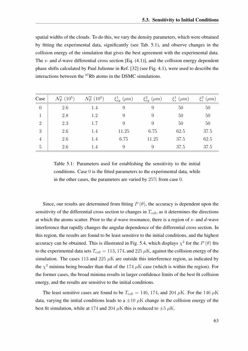
5.3. Sensitivity to Initial Conditions
spatial widths of the clouds. To do this, we vary the density parameters, which were obtained
by fitting the experimental data, significantly (see Tab. 5.1), and observe changes in the
collision energy of the simulation that gives the best agreement with the experimental data.
The s- and d-wave differential cross section [Eq. (4.1)], and the collision energy dependent
phase shifts calculated by Paul Julienne in Ref. [32] (see Fig. 4.1), were used to describe the
interactions between the 87Rb atoms in the DSMC simulations.
Case N 1P (105) N 2
P (105) ξ1xy (µm) ξ2
xy (µm) ξ1z (µm) ξ2
z (µm)
0 2.6 1.4 9 9 50 50
1 2.8 1.2 9 9 50 50
2 2.3 1.7 9 9 50 50
3 2.6 1.4 11.25 6.75 62.5 37.5
4 2.6 1.4 6.75 11.25 37.5 62.5
5 2.6 1.4 9 9 37.5 37.5
Table 5.1: Parameters used for establishing the sensitivity to the initial
conditions. Case 0 is the fitted parameters to the experimental data, while
in the other cases, the parameters are varied by 25% from case 0.
Since, our results are determined from fitting P (θ), the accuracy is dependent upon the
sensitivity of the differential cross section to changes in Tcoll, as it determines the directions
at which the atoms scatter. Prior to the d-wave resonance, there is a region of s- and d-wave
interference that rapidly changes the angular dependence of the differential cross section. In
this region, the results are found to be least sensitive to the initial conditions, and the highest
accuracy can be obtained. This is illustrated in Fig. 5.4, which displays χ2 for the P (θ) fits
to the experimental data sets Tcoll = 113, 174, and 225 µK, against the collision energy of the
simulation. The cases 113 and 225 µK are outside this interference region, as indicated by
the χ2 minima being broader than that of the 174 µK case (which is within the region). For
the former cases, the broad minima results in larger confidence limits of the best fit collision
energy, and the results are sensitive to the initial conditions.
The least sensitive cases are found to be Tcoll = 146, 174, and 204 µK. For the 146 µK
data, varying the initial conditions leads to a ±10 µK change in the collision energy of the
best fit simulation, while at 174 and 204 µK this is reduced to ±5 µK.
63
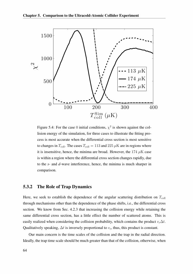
Chapter 5. Comparison to the Ultracold-Atomic Collider Experiment
χ2
T Simcoll (µK)
100 200 300 4000
500
1000
1500
113 µK
174 µK
225 µK
Figure 5.4: For the case 0 initial conditions, χ2 is shown against the col-
lision energy of the simulation, for three cases to illustrate the fitting pro-
cess is most accurate when the differential cross section is most sensitive
to changes in Tcoll. The cases Tcoll = 113 and 225 µK are in regions where
it is insensitive, hence, the minima are broad. However, the 174 µK case
is within a region where the differential cross section changes rapidly, due
to the s- and d-wave interference, hence, the minima is much sharper in
comparison.
5.3.2 The Role of Trap Dynamics
Here, we seek to establish the dependence of the angular scattering distribution on Tcoll
through mechanisms other than the dependence of the phase shifts, i.e., the differential cross
section. We know from Sec. 4.2.3 that increasing the collision energy while retaining the
same differential cross section, has a little effect the number of scattered atoms. This is
easily realized when considering the collision probability, which contains the product vr∆t.
Qualitatively speaking, ∆t is inversely proportional to vr, thus, this product is constant.
Our main concern is the time scales of the collision and the trap in the radial direction.
Ideally, the trap time scale should be much greater than that of the collision, otherwise, when
64

5.3. Sensitivity to Initial Conditions
the system is imaged quarter the radial trap period after the clouds overlap, the collision may
not yet be complete (the clouds still spatially overlap). This can be seen in Fig. 5.5, which
shows the fraction of total scattered atoms to the total number of atoms (N 1sc +N 2
sc) /NP (the
superscript indicates which cloud). Below Tcoll = 100 µK the number of scattered atoms
decreases with decreasing Tcoll. However, in this region, the total cross section increases (see
Fig. 4.1) with decreasing Tcoll, which is expected to cause an increase in scattered atoms.
( N1 sc+
N2 sc
) /N
P
T Simcoll (µK)
100 200 300 4000
0.1
0.2
0.3
0.4
0.5
Figure 5.5: The total fraction of scattered atoms for the fitted set of initial
conditions (Case 0) against the collision energy of the simulation. The
solid black line gives scattered fraction for both groups (i) and (ii), while
the dashed black line gives group (i), and dashed-dotted black line gives
group (ii). The groups are defined as in Sec. 4.2.3: (i) scattered atoms that
have not undergone any subsequent collisions, (ii) scattered atoms that
have undergone additional collisions, including all collision partners.
In the extreme case, where the collision time scale is much greater than the trap time
scales, atoms that scatter at the beginning of the collision, may undergo multiple trap oscil-
lations in the radial direction. This is not ideal, as the angular distribution of scattered atoms
becomes difficult to measure. Provided we concern ourselves with collision energy regimes
Tcoll > 100 µK, these issues will be less of a concern, as increasing Tcoll (increasing the
relative speed of the clouds) diminishes the collision timescale.
65
Chapter 5. Comparison to the Ultracold-Atomic Collider Experiment
For the cases we wish to consider, the 146 µK case has a small dependence on these
issues, while for 174 and 204 µK, these issues have negligible effect, i.e., the dependence on
Tcoll is solely through the differential cross section.
5.3.3 Summary of Important Results
We have seen that the experimental scattering patterns for Tcoll = 146, 174, and 204 µK are
insensitive to the initial conditions, hence, suitable for us to focus our attention upon. These
cases all occur in a regime where there is significant s- and d-wave interference, with the
phase shifts varying rapidly with collision energy.
We have also seen that the results are largely insensitive to the collision energy of the
simulation, except through the collision energy dependence of the differential cross section.
5.4 Results
In this section we present the main results of the chapter. We first apply the DSMC method
to provide a quantitative model of the experiments, using the partial-wave phase shifts pre-
dicted by Paul Julienne. Our results show significant disagreement between the theoretical
and experimental results suggesting that the theoretical phase shifts are inconsistent with
experiment. From our simulations, we infer that the location of the d-wave resonance is
significantly lower than Paul Julienne’s, and more recently, Eite Tiesinga’s predictions (see
Sec. 5.1). We also use these simulations to investigate the role of the many-body dynamics
in the experimental data, and show that a simple differential cross section model is inappro-
priate for providing a quantitative model of this experimental regime.
Motivated by the inadequacy of the current two-body predictions, we establish a model
differential cross section to simulate experiments, and quantitatively determine the partial-
wave phase shifts at Tcoll = 174 µK.
66
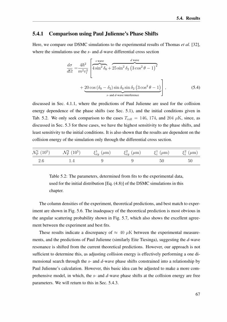
5.4. Results
5.4.1 Comparison using Paul Julienne’s Phase Shifts
Here, we compare our DSMC simulations to the experimental results of Thomas et al. [32],
where the simulations use the s- and d-wave differential cross section
dσ
dΩ=
4~2
m2v2r
s wave︷ ︸︸ ︷4 sin2 δ0 +
d wave︷ ︸︸ ︷25 sin2 δ2
(3 cos2 θ − 1
)2
+ 20 cos (δ0 − δ2) sin δ0 sin δ2
(3 cos2 θ − 1
)︸ ︷︷ ︸
s- and d-wave interference
, (5.4)
discussed in Sec. 4.1.1, where the predictions of Paul Julienne are used for the collision
energy dependence of the phase shifts (see Sec. 5.1), and the initial conditions given in
Tab. 5.2. We only seek comparison to the cases Tcoll = 146, 174, and 204 µK, since, as
discussed in Sec. 5.3 for these cases, we have the highest sensitivity to the phase shifts, and
least sensitivity to the initial conditions. It is also shown that the results are dependent on the
collision energy of the simulation only through the differential cross section.
N 1P (105) N 2
P (105) ξ1xy (µm) ξ2
xy (µm) ξ1z (µm) ξ2
z (µm)
2.6 1.4 9 9 50 50
Table 5.2: The parameters, determined from fits to the experimental data,
used for the initial distribution [Eq. (4.8)] of the DSMC simulations in this
chapter.
The column densities of the experiment, theoretical predictions, and best match to exper-
iment are shown in Fig. 5.6. The inadequacy of the theoretical prediction is most obvious in
the angular scattering probability shown in Fig. 5.7, which also shows the excellent agree-
ment between the experiment and best fits.
These results indicate a discrepancy of ≈ 40 µK between the experimental measure-
ments, and the predictions of Paul Julienne (similarly Eite Tiesinga), suggesting the d-wave
resonance is shifted from the current theoretical predictions. However, our approach is not
sufficient to determine this, as adjusting collision energy is effectively performing a one di-
mensional search through the s- and d-wave phase shifts constrained into a relationship by
Paul Julienne’s calculation. However, this basic idea can be adjusted to make a more com-
prehensive model, in which, the s- and d-wave phase shifts at the collision energy are free
parameters. We will return to this in Sec. 5.4.3.
67

Chapter 5. Comparison to the Ultracold-Atomic Collider Experiment
146 µK
174 µK
204 µK
146 µK
174 µK
204 µK
190 µK
205 µK
245 µK
Experiment Theory Best Fit
250 µm
Figure 5.6: The experimental column densities are displayed in the first
column, while the theoretical predictions (DSMC simulations furnished
with the two-body calculations of the s- and d-wave phase shifts) are
displayed in the second column. The collision energy of the experi-
ment/simulation is displayed in the bottom right corner of each image.
The best matches to the experimental data is to the right of the experimen-
tal data in the third column. These show a discrepancy of 30 − 40 µK
between the collision energy of experiment and of theory. The confidence
limits for the collision energy of the best fit for the 146 µK case is ±10
µK, while ±5 µK for the other two cases.
68
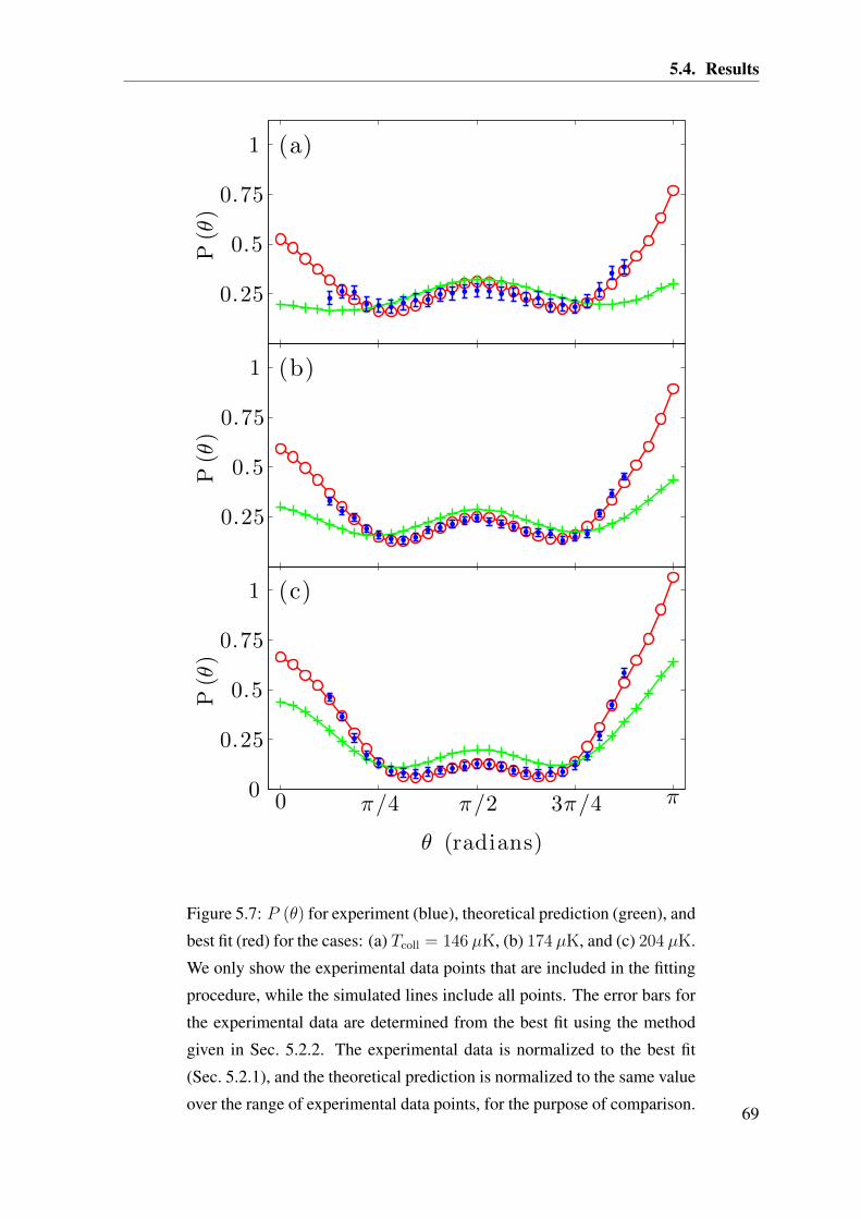
5.4. Results
θ (radians)
P(θ
)
0 π/4 π/2 3π/4 π0
0.25
0.5
0.75
1
P(θ
)
0.25
0.5
0.75
1
P(θ
)
0.25
0.5
0.75
1 (a)
(b)
(c)
Figure 5.7: P (θ) for experiment (blue), theoretical prediction (green), and
best fit (red) for the cases: (a) Tcoll = 146 µK, (b) 174 µK, and (c) 204 µK.
We only show the experimental data points that are included in the fitting
procedure, while the simulated lines include all points. The error bars for
the experimental data are determined from the best fit using the method
given in Sec. 5.2.2. The experimental data is normalized to the best fit
(Sec. 5.2.1), and the theoretical prediction is normalized to the same value
over the range of experimental data points, for the purpose of comparison. 69
Chapter 5. Comparison to the Ultracold-Atomic Collider Experiment
5.4.2 Necessity of the DSMC method
Inadequacy of Differential Cross Section Analysis
The simple two-body approach of using the s- and d-wave differential cross section [Eq. (5.4)]
itself as the fitting model for P (θ) does not provide a quantitative model of the experimen-
tal data, as the many-body effects are significantly large. For example, Fig. 5.8 compares
the best fits of the DSMC simulation (as discussed in Sec. 5.4.1), and the differential cross
section, to the experimental data for the case of Tcoll = 174 µK. Notably, using this simple
model increases the discrepancy found between the experimental collision energy and best
match using Paul Julienne’s prediction for the phase shifts (see Sec. 5.4.1) from ≈ 40 µK to
≈ 60 µK.
In the following, we examine the underlying physics that makes the differential cross
section analysis inapplicable. Finally, we discuss the changes that would be required for the
collider experiments to operate in a regime where differential cross section analysis could be
used.
Many-Body and Finite Size Effects
Since, the trap dynamics are mostly accounted for in the procedure to determine the angular
scattering probability (see Fig. 5.2, and Sec. 5.2.1), and the results are only dependent upon
the collision energy through the differential cross section for Tcoll > 100 µK (see Sec. 5.3.2),
it is primarily atoms undergoing multiple collisions, and the finite sizes of the clouds, which
cause the differential cross section analysis to be inapplicable. Indeed, the differential cross
section analysis would be exact provided all the collisions occurred at the same point in space
and time (i.e., no finite size effects), and the scattered atoms did not undergo any subsequent
collisions.
The most important many-body effect, is atoms undergoing multiple collisions after the
initial outscattering collision. This can significantly change the trajectory of the outscattered
atoms, and causes asymmetries in the initial clouds to be resolved in P (θ) (e.g., see Fig. 5.7).
The second source is the finite sizes of the clouds. This causes collisions to occur over a range
of times and positions, which has the effect of broadening the collision halo.2
2Multiple collisions also broaden the collision halo.
70

5.4. Results
θ (radians)
P(θ
)
0 π/4 π/2 3π/4 π0
0.25
0.5
0.75
Figure 5.8: P (θ), for the case of Tcoll = 174 µK, is shown for experiment
(blue), the best fit of the differential cross section (green), and the best
fit of the DSMC simulations of Sec. 5.4.1. This demonstrates that the
differential cross section is a poor model for this experimental regime.
The differential cross section model yields a best fit collision energy of
228 µK. We do not include the confidence limits, as the requirement that
the model is appropriate for the "goodness-of-fit" in Sec. 5.2.2 is no longer
fulfilled.
71

Chapter 5. Comparison to the Ultracold-Atomic Collider Experiment
Minimizing the Many-Body and Finite Size Effects
The effects that cause the differential cross section to be a poor model for the fit, can be
negated by changing the experimental set up in several ways. First, reducing the density of
the clouds, so that, fewer collisions occur. How much of a reduction, and how to best achieve
this, is given qualitatively by Fig. 4.9 and Eq. (4.18),
Nsc =N 2
P
4πmβωxωyσ0. (5.5)
Equation (5.5) is not accurate for Nsc/NP > 0.05, but it qualitatively illustrates how a
reduction in the density, reduces the scattering fractions. In Fig. 4.9, our results showed that
for scattering fractions less than 15%, relatively few second collisions occurred.
The finite sizes of the clouds, become less important with increasing distance between
the atoms when imaged and the collision site. Hence, one can use a weaker trap in the radial
direction, or turn the trap off during, or after, the clouds collide. However, the imaging
capabilities of the experiment must be kept in mind, since the density of the scattered atoms
decreases as the collision halo expands.
5.4.3 Two-Parameter Model for Fitting to the Experiments
As we have shown in the previous sections, the current theoretical model for the partial-
wave phase shift collision energy dependence is not in agreement with experiment, thus, we
are motivated to give quantitative measures of the phase shifts from the experimental data.
Here, we first introduce a model appropriate for performing such measurement, and then,
give quantitative results of the experimental data at the collision energy of Tcoll = 174 µK.
The Model Differential Cross Section
Determining the simulation collision energy that most closely matches the experimental re-
sult is not a sufficiently general description to determine the phase shifts, since, this is a
single parameter search (in terms of collision energy), and does not allow the s- and d-wave
phase shifts to vary independently.
Here, we will concentrate on the Tcoll = 174 µK case, since the angular scattering prob-
ability is most sensitive to changes the phase shifts, giving the most accurate results. In
the simulation, the collision energy of the clouds is taken to be T Simcoll = 174 µK, and we
introduce a model, where all collisions occuring with Tcoll ≤ 0.95T Simcoll = 165.3 µK, are
described by the low energy s-wave (isotropic) differential cross section. For collisions oc-
curring with Tcoll > 0.95T Simcoll , we use the s- and d-wave differential cross section, with the
72

5.5. Conclusion
constant phase shifts δ0 and δ2 (the fitting parameters). I.e.,
dσ
dΩ=
8πa2sc T ijcoll ≤ 0.95T Sim
coll ,
D(θ, δ0, δ2
)T ijcoll > 0.95T Sim
coll ,(5.6)
where D indicates the s- and d-wave differential cross section [Eq. (5.4)], and ij indicates
the colliding pair of test particles. The rational of model (5.6) is as follows: It ensures
that low-energy collisions (e.g., collision within each cloud) occur at the background low-
energy cross section. However, a majority of high-energy collisions between the clouds
occur with T ijcoll ≈ T Simcoll , and these contribute most significantly to the angular scattered
distribution. Thus, for these collisions (T ijcoll > 0.95T Simcoll ), we take the phase shifts to be
constant parameters, which form the basis of our fitting procedure.
We have already established that a significant number of atoms undergo multiple inter-
collisions, which occur at various T ijcoll (most are close to T Simcoll ). Thus, we test this model
by comparing it to the simulated results of Sec. 5.4.1 for the cases of Tcoll = 174, and 205
µK, which include the full collision energy dependence of the phase shifts. These are the
collision energy of the the simulations undertaken here, and the best fit from that section for
the experimental results of 174 µK (e.g., see Fig. 5.8), respectively. This comparison is done
by takingδ0, δ2
=δ0
(T icoll
), δ2
(T icoll
), (5.7)
for the model differential cross section 5.6, where T icoll refer to the two cases above, and
the Tcoll dependence is the same as that used in Sec. 5.4.1 (i.e., Paul Julienne’s predictions).
The Fig. 5.9 shows good agreement for this comparison, indicating our choice of model is
sufficient to describe the regime of interest for the collider.
Best Fits and Corresponding Phase Shifts
By performing simulations for a range of δ0 and δ2, the best fits to the experimental data (see
Fig. 5.10) are given by the phase shifts in Tab. 5.3. We find that the partial-wave predictions
of Paul Julienne, and Eite Tiesinga in Sec. 5.1, give very good agreement for the s-wave
phase shift, however, the d-wave phase shift is significantly different.
5.5 Conclusion
Our DSMC simulations have shown there is a serious discrepancy between theoretical pre-
dictions for the phase shifts of 87Rb in the 200 µK regime. By developing an adjustable
73

Chapter 5. Comparison to the Ultracold-Atomic Collider Experiment
θ (radians)
P(θ
)
0 π/4 π/2 3π/4 π0
0.25
0.5
0.75
P(θ
)
0.2
0.4
0.6 (a)
(b)
Figure 5.9: The red lines indicate the simulated results of Sec. 5.4.1 for
the cases of T Simcoll = 174 (a), and 205 (b) µK. These results use the full
collision energy dependence shown in Fig. 4.1. The blue lines are given
by the s-wave cutoff model of this section. The good agreement shows
that this simplified model is sufficient.
74

5.5. Conclusion
θ (radians)
P(θ
)
0 π/4 π/2 3π/4 π0.1
0.2
0.3
0.4
0.5
Figure 5.10: Comparison of the best fit of Sec. 5.4.1 (green), and the
s-wave cutoff model of this section (red), to the experimental data for
Tcoll = 174 µK (blue). We only plot P (θ) over the considered range of
the experimental P (θ), to highlight the quality of the agreement. The
least-squares residual for case (a) is 0.0080, while for case (b) it is 0.0067.
75

Chapter 5. Comparison to the Ultracold-Atomic Collider Experiment
TExptcoll δFit
0 δFit2 δA0 δA2 δB0 δB2
174 −0.97± 0.08 0.52± 0.02 −0.97 0.23 −0.97 0.23
Table 5.3: Here the fitted partial-wave phase shifts δFiti , and phase shifts
calculated by Eite Tiesinga (δAi ), and Paul Julienne (δBi ), are shown, where
i = 0, 2. At this collision energy (Tcoll = 174 µK), the two theoreti-
cal calculations agree to two significant figures. We find good agreement
with the s-wave phase shift. However, the d-wave phase shift disagrees
significantly.
model for the phase shifts, we have determined that this discrepancy lies mostly in the deter-
mination of the d-wave phase shift, and we have been able to provide a measure of the phase
shifts at 174 µK to an accuracy that should be a constraint in future two-body calculations to
improve our knowledge of the inter-atomic potentials.
The techniques that we have developed and applied, demonstrate that the ultracold-
atomic collider (with appropriate theoretical analysis) can provide a tool for precision colli-
sion spectroscopy.
76

Chapter 6
Extension of DSMC to Include QuantumMany-Body Statistics
In this chapter, we discuss extending the DSMC method to the quantum many-body descrip-
tion given by the quantum Boltzmann equation. First, we derive the quantum many-body
collision probability, and then, show how the algorithm presented in Chapter 3 is modified to
accommodate this new collision probability. Then, we discuss the problems associated with
constructing f (p, r, t) during runtime, which is of crucial importance to the accuracy of
the simulation. We suggest several new constructions of f (p, r, t) to remedy this currently
unsolved problem.
6.1 Derivation of the Quantum Collision Probability
Jackson and Zaremba [18] showed that the collision probability may be derived by treating
the test particles as an accepted set of samples for the Monte Carlo integration of the collision
rate per unit volume,
R (r, t) =1
m
∫d6u
h6
∫dΩ
dσ
dΩ|p1 − p| ff1 (1± f ′) (1± f ′1) , (6.1)
where d6u = d3p d3p1. Deriving the collision probability in this fashion directly links the
collisions of the test particles to the collision integral [Eq. (2.4)], and gives insight as to
how the test particles function to solve the quantum BE. It also shows how the quantum
many-body statistics are incorporated into the collision probability without resorting to ad
hoc arguments. This result provides a useful framework to discuss the quantum extension of
DSMC in detail. We now follow their methodology, and, where relevant to our purposes, we
discuss details and make adjustments.
77

Chapter 6. Extension of DSMC to Include Quantum Many-Body Statistics
Rewriting Eq. (6.1) as
R (r, t) =
∫d6u
h6w (u, r, t) g (u, r, t) , (6.2)
where u is a point in the six-dimensional momentum hyper-space, and the weight function
is
w (u, r, t) ≡ ff1, (6.3)
and
g (u, r, t) =1
m
∫dΩ
dσ
dΩ|p1 − p| (1± f ′) (1± f ′1) . (6.4)
If the integrand is non-zero on the domain[−pmax
2, pmax
2
]for each of the six momentum
components, we may approximate the integral by Monte Carlo integration with the following
process: randomly select a point ui in the non-zero domain of the integrand and randomly
select a numberwi in the range [0, wmax], wherewmax is the maximum of the weight function.
If wi < w (ui, r, t) then the point ui is accepted. By repeating this N times, the approximate
solution to the integral is given by
R (r, t) ' (pmax)6wmax1
N
Nacc∑
i=1
g (uacci , r, t) , (6.5)
where the summation is over only the accepted points uacci , hence, Nacc ≤ N is the number
of such accepted points. If g (u, r, t) = 1, then, the integral would equate to the square of
the density, i.e.,
n (r, t)2 =
∫d6u
h6ff1, (6.6)
and thus, we may write
n (r, t)2 ' (pmax)6wmaxNacc
N. (6.7)
Using this, we can rewrite Eq. (6.5) as
R (r, t) ' n (r, t)2 1
Nacc
Nacc∑
i=1
g (uacci , r, t) . (6.8)
The momenta, p and p1, in the set of Nacc accepted points u = (p,p1) are distributed
according to f (p, r, t). Since, the test particles are also distributed according to f (p, r, t),
they can form the set of accepted Monte Carlo samples. However, there are a limited number
of test particles representing f (p, r, t), demanding we take a reasonable cell volume about r
to ensure enough test particles to implement Eq. (6.8). Two important questions we address
later are:
(i) What considerations are important in deciding the cell volume?
78
6.1. Derivation of the Quantum Collision Probability
(ii) What value of n (r, t) should be used for a finite cell volume?
Using Eq. (6.8), the number atoms which undergo a collision within the cell volume ∆V
about the point r in the time interval t to t+ ∆t is approximately
Ncoll ' n (r, t)2 1
Nacc
Nacc∑
i=1
g (uacci , r, t) ∆V∆t, (6.9)
Here we have assumed that the density across the volume is constant, thus, regardless of the
approach taken for questions (i) and (ii) we may write n (r, t) = 2αNacc/∆V , where we
have taken the number of atoms in that volume to be 2Nacc (i.e., we have used the 2Nacc test
particles to provide Nacc samples of p, and Nacc samples of p1). Using this, and the fact that
the number of test particles which undergo a collision is Ncoll = Ncoll/α, since each atom is
represented by 1/α test particles, one arrives at
Ncoll ' 2n (r, t)Nacc∑
i=1
g (uacci , r, t) ∆t. (6.10)
Thus, we may associate a collision probability Pij , for the pairs of test particles within the
volume,
Pij = n (r, t) g (uacci , r, t) ∆t = n (r, t) vrσeff∆t, (6.11)
where the factor of 2 has been dropped as two test particles participate in the collision, and i
and j refer to the individual test particles of a given pair. The effective total cross section is
given by
σeff =
∫dΩ
dσ
dΩ(1± f ′) (1± f ′1) . (6.12)
We now return to the questions (i) and (ii) posed earlier: We have seen that regardless
of the choices for the cell volume and n (r, t), we arrive at the same collision probability
for testing Nacc = n (r, t) ∆V/2α collisions. Thus, the choices only have an effect on how
well n (r, t), f ′, and f ′1 are represented, and hence, the accuracy of the simulation. Here,
we consider three different choices: (1) the original DSMC method, (2) the NNC scheme,
and (3) a scheme we call locally sampled density (LSD). The relevant characteristics of the
schemes are shown in Tab. 6.1. Before we introduce the LSD scheme, it is useful to discuss
the first two.
In the original DSMC method, ∆V = ∆Vc, and the density is the average density of
the cell nc. The current form (Pij given by Eq. (6.11) and Nacc = Nc/2) corresponds to
Mc = N2c /2 collisions. In light of the discussions in Sec. 3.3.3, we know that this derivation
should be modified, such that, Mc = Nc (Nc − 1) /2, which is done by now taking Nacc =
(Nc − 1) /2. Thus, this choice reduces Eq. (6.11) to exactly that of which is obtained by
79

Chapter 6. Extension of DSMC to Include Quantum Many-Body Statistics
Scheme ∆V n (r, t)
Original DSMC ∆Vc nc
NNC 2α/nc nc
LSD 2α/n (rcom, t) n (rcom, t)
Table 6.1: Choices for ∆V and n (r, t) for the different schemes.
Bird [35], Eq. (3.10), with the appropriate scaling for Eqs. (3.12), and σ (vr) = σeff . The
NNC scheme can be understood as restricting ∆V to the volume, which on average for the
collision cell, contains only two test particles, however, retaining the density to be nc.
We have developed the LSD scheme, which restricts ∆V to contain two test particles
using the (yet to be determined) density evaluated at the centre-of-mass n (rcom, t). This
density could be obtained via an ansatz for the density or the interpolation of all test particles
in the simulation or in the cell itself. However, if n (rcom, t) is determined from the test
particles, it can reintroduce the finite number fluctuation issues discussed in Sec. 3.3.3, and
we find for the classical DSMC algorithm, this disadvantage is significant enough that it
should not be used. The fluctuation issues can, ofcourse, be circumvented by using more
test particles. However, we shall see later in Sec. 6.3 that the quantum extension of DSMC
requires large cells for many test particles, which causes nc to be a very coarse grained
representation. Here, the LSD scheme is expected to be most useful, as it can remove this
coarse graining, giving potentially more accurate simulations.
6.2 Adjustments to the DSMC Algorithm
Here, we discuss how the addition of the quantum many-body component changes the clas-
sical DSMC algorithm we presented in Chapter 3.
6.2.1 Scaling and LATS
Scaling of the collision probability and number of tested collisions is discussed in Sec. 3.3.3.
Pij → Pij =PijΛ, (6.13a)
Mc → Mc = McΛ, (6.13b)
is now given with
Λ =dMc∆t [n (r, t) vrσeff ]maxe
Mc
. (6.14)
80

6.2. Adjustments to the DSMC Algorithm
For computational simplicity and performance, we take
[n (r, t) vrσeff ]max = nmax [1 + εfmax]2 [vrσ (vr)]max , (6.15)
where nmax and fmax are the maximum values within the cell, and ε = 1 (0) for bosons
(fermions). Thus,
Pij =Mcn (r, t) vrσeff∆t⌈
Mc∆tnmax [1 + εfmax]2 [vrσ (vr)]max
⌉ . (6.16)
Finally, for the LATS scheme, the relevant collision times of a cell are now given by
τ collc = n (r, t) vrσeff
−1, (6.17a)
τmaxc =
nmax [1 + εfmax]2 [vrσ (vr)]max
−1. (6.17b)
6.2.2 Testing and Implementation of Collisions
The evaluation of Pij is more involved, due to the addition of the integral
σeff =
∫dΩ
dσ
dΩ(1± f ′) (1± f ′1) . (6.18)
During runtime, this integral must be evaluated, which, analytically, is almost always in-
tractable, and the analytical solutions can often be infeasible to implement numerically.1
Then, if the test particles collide, they scatter at angles determined by dσdΩ
(1± f ′) (1± f ′1).
We can combined these procedures into one, by employing the Monte Carlo method of staked
probabilities. This gives an approximate solution to Eq. (6.18), while determining the scat-
tering angles of the particles if they collide. The collision probability is taken to be
Pij =2π
Ns
Ns∑
k=1
PΩkij , (6.19)
where Ns is the number of samples, and
PΩkij =
n (r, t) vr∆t
Λ
[dσ
dΩ(1± f ′) (1± f ′1)
]Ωk
, (6.20)
with [x]Ωk indicating that x is evaluated at the randomly selected angles Ωk. The collision
goes ahead if R < Pij , where R is a random number uniformly distributed between 0 and 1,
and the scattering angles are given as Fig. 6.1 demonstrates.
1For example, Eq. (6.18) can be solved for the equilibrium Bose-Einstein distribution, however, the solution
is an infinite sum.
81
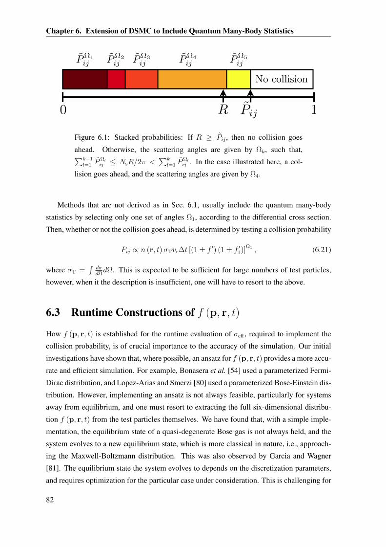
Chapter 6. Extension of DSMC to Include Quantum Many-Body Statistics
PΩ1ij PΩ2
ij PΩ3ij PΩ4
ij PΩ5ij
No collision
0 1R PijPij
Figure 6.1: Stacked probabilities: If R ≥ Pij , then no collision goes
ahead. Otherwise, the scattering angles are given by Ωk, such that,∑k−1
l=1 PΩlij ≤ NsR/2π <
∑kl=1 P
Ωlij . In the case illustrated here, a col-
lision goes ahead, and the scattering angles are given by Ω4.
Methods that are not derived as in Sec. 6.1, usually include the quantum many-body
statistics by selecting only one set of angles Ω1, according to the differential cross section.
Then, whether or not the collision goes ahead, is determined by testing a collision probability
Pij ∝ n (r, t)σTvr∆t [(1± f ′) (1± f ′1)]Ω1 , (6.21)
where σT =∫
dσdΩdΩ. This is expected to be sufficient for large numbers of test particles,
however, when it the description is insufficient, one will have to resort to the above.
6.3 Runtime Constructions of f (p, r, t)
How f (p, r, t) is established for the runtime evaluation of σeff , required to implement the
collision probability, is of crucial importance to the accuracy of the simulation. Our initial
investigations have shown that, where possible, an ansatz for f (p, r, t) provides a more accu-
rate and efficient simulation. For example, Bonasera et al. [54] used a parameterized Fermi-
Dirac distribution, and Lopez-Arias and Smerzi [80] used a parameterized Bose-Einstein dis-
tribution. However, implementing an ansatz is not always feasible, particularly for systems
away from equilibrium, and one must resort to extracting the full six-dimensional distribu-
tion f (p, r, t) from the test particles themselves. We have found that, with a simple imple-
mentation, the equilibrium state of a quasi-degenerate Bose gas is not always held, and the
system evolves to a new equilibrium state, which is more classical in nature, i.e., approach-
ing the Maxwell-Boltzmann distribution. This was also observed by Garcia and Wagner
[81]. The equilibrium state the system evolves to depends on the discretization parameters,
and requires optimization for the particular case under consideration. This is challenging for
82

6.3. Runtime Constructions of f (p, r, t)
nonequilibrium systems, e.g., for the collisions of ultracold degenerate clouds, for which, the
optimized parameters for the initial and final states can be different. Ideally, the algorithm
should be robust and stand alone, or the discretization effects well understood and easily ac-
counted for. However, this is largely an unexplored problem, with the exception of the study
of Garcia and Wagner [81], and is often overlooked by people working in this area.2 Here,
we do not solve this problem, but present several possible avenues of investigations.
6.3.1 Analytic Result Required for Test of Collision Rate
Until now, the tests we performed on our (classical) DSMC algorithm were largely concerned
with giving the correct collision rate (see Sec. 4.2). This is a necessary requirement for the
accuracy of the simulation, but not sufficient in the quantum many-body context. The testbed
distribution for the collision rate is a degenerate case of the Bose-Einstein distribution
f (p, r) =1
exp β [H (p, r)− µ] − 1=∞∑
j=1
exp jβ [µ−H (p, r)] , (6.22)
where H is the Hamiltonian of the system. Using the Gaussian expansion, we can solve for
the collision rate [Eq. (6.1)], yielding
R (r) =1
2√
2~6
σ1
m
(m
πβ
) 72∞∑
j,k=1
exp β [j + k] [µ− U(r)]×
1
jk
[√j + k
jk+ 2
∞∑
l=1
√j + k + l
(j + l) (k + l)exp lβ [µ− U(r)]
]+
∞∑
l,n=1
√j + k + l + n
(j + l) (k + l) (j + n) (k + n)exp β [l + n] [µ− U(r)]
, (6.23)
where we have assumed a constant differential cross section that yields the total cross section
σ1. This result was also found by Lopez-Arias and Smerzi [80]. For a harmonic potential,
2For methods based on molecular dynamics like closest-approach collisions, which the closest-approach
distance does not scale with NT, it is unclear whether one should be concerned with this, since these methods
ultimately do not solve the quantum BE (assumes point particle collisions).
83

Chapter 6. Extension of DSMC to Include Quantum Many-Body Statistics
integrating over each position space direction is relatively simple, and gives
R =1
ωxωyωz
1
~6
mσ1
π2β5
∞∑
j,k=1
exp [β (j + k)µ]×
1
jk
[1
jk
1
(j + k)+ 2
∞∑
l=1
1
(j + l) (k + l)
1
(j + k + l)exp [lβµ]
]+
∞∑
l,n=1
1
(j + l) (k + l) (j + n) (k + n)
1
(j + k + l + n)exp [β (l + n)µ]
. (6.24)
These expressions can be evaluated numerically, and give us a benchmark to test the initial
accuracy of the DSMC simulation. However, initially the agreement between the analytical
collision rate and the numerical collision rate determined by DSMC can be very good, but
when the system is evolved in time, it can still progressively evolve away from the initial
distribution. This must be checked for, in conjunction with the collision rate.
6.3.2 Three Constructions
For systems away from equilibrium, it is not always feasible to use an ansatz for f (p, r, t),
thus, one must resort to establishing f (p, r, t) from the test particles. We present three
constructions of f (p, r, t), the first being the typical construct found in literature, and the
other two, suggestions we make to combat issues discussed in due course. We also discuss
the mechanism that causes the system to evolve away from the initial state.
Construction (c1):
The simplest construction of f (p, r, t) is the mean density of the cell multiplied by a nor-
malized momentum distribution obtained from the test particles within the cell Kc (p, t),
fc (p, t) = ncKc (p, t) , (6.25)
where ∫d3p
h3Kc (p, t) = 1. (6.26)
Kc (p, t) can be determined binning the test particles into a grid of cells in momentum space
with width ∆pi in the i = (x, y, z) direction. This can be performed in several ways, e.g.,
the particles can be mapped to the nearest grid point (the so called nearest grid point or
84

6.3. Runtime Constructions of f (p, r, t)
zeroth order scheme), and the resulting distribution convoluted with a Gaussian function.
The convolution theorem allows the convolution to be easily performed in Fourier space,
however, performing a Fast Fourier Transform (FFT), and then, the inverse-FFT for each
cell is computationally taxing. We find that similar accuracy can be achieved with the higher
order interpolation schemes of Ref. [78], and in most cases, for less computational effort.
Construction (c2):
For construction (c1), Kc (p, t) requires Nc to be large for a sufficiently accurate description,
hence, large ∆Vc, causing the density to be coarsely grained. The first new construction we
suggest, is to use the LSD scheme for the density,
fc (p, t) = n (rcom, t)Kc (p, t) . (6.27)
n (rcom, t) can be established by the convolution or interpolation methods as discussed for
Kc (p, t) above. This will give a more accurate description of the density, but, as we noted
earlier, this can reintroduce the fluctuation issues discussed in Sec. 3.3.3. However, we note
that the form of construction (c1) [Eq. (6.25)] does not remove these issues in the quantum
many-body description, since the product
n (r, t) (1± f ′) (1± f ′1) , (6.28)
in the collision probability is not linear in n (r, t). Furthermore, the fluctuation issues may
be less significant, as we require large Nc for Kc (p, t).
Construction (c3):
A careful study is required to determine whether the coarse graining of construction (c1), or
fluctuation issues in both constructions (c1) and (c2), will be important. However, our initial
investigations suggest that the fluctuations are most important in both cases. Furthermore,
this causes the two problems: (a) accurately representing the collision rate, and (b) the pro-
gressive evolution to another state, to be coupled. This motivates us to extend the methods
of Sec. 3.3.3 to remove the fluctuation issues, and uncouple the problems. For Eq. (6.25),
Eq. (6.28) reads
nc ± n2c [Kc (p′, t) +Kc (p′1, t)] + n3
cKc (p′, t)Kc (p′1, t) , (6.29)
85
Chapter 6. Extension of DSMC to Include Quantum Many-Body Statistics
thus, the collision rate features N2c , N3
c , and N4c . For Poissonian distributed fluctuations, one
can show
Nc (Nc − 1)∗
= Nc2, (6.30a)
Nc [Nc (Nc − 3) + 1]∗
= Nc3, (6.30b)
Nc Nc [Nc (Nc − 6) + 11]− 6∗ = Nc4, (6.30c)
where the asterisks indicates we have taken into account that the DSMC simulation neglects
cells with single occupation. Thus, the fluctuation affects can be removed by taking Mc =
Nc/2, and by replacing Eq. (6.29) with
ϑ (Nc − 1)± ϑ2 [Nc (Nc − 3) + 1] [Kc (p′, t) +Kc (p′1, t)] +
ϑ3 Nc [Nc (Nc − 6) + 11]− 6Kc (p′, t)Kc (p′1, t) , (6.31)
where ϑ = α/∆Vc, giving our second suggested construction. In detail, this gives
Pij = vr∆t
∫dΩ
dσ
dΩϑ [(Nc − 1)± ϑ [Nc (Nc − 3) + 1] [Kc (p′, t) +Kc (p′1, t)] +
ϑ2 Nc [Nc (Nc − 6) + 11]− 6Kc (p′, t)Kc (p′1, t)]. (6.32)
We have neglected the fact that Kc (p′, t) and Kc (p′1, t) are also determined from the test
particles, hence, have correlated fluctuations. The fluctuations may not have a significant
effect, and they may be negated by the scheme which established Kc (p, t).
Mechanism for Unphysical Evolution
We now discuss the mechanism that causes the system to progressively evolve away from
the initial equilibrium state. This artificial evolution is due to the transfer of information
in the collisions of test particles. The NNC scheme, which was introduced in a classical
context, combats transfer of information of spatially separated collision partners, however,
with the inclusion of quantum many-body statistics [(1± f ′) (1± f ′1)], there is now another
mechanism which destroys the correlations. We are concerned with the final states to which
the test particles scatter, which is determined by dσdΩ
(1± f ′) (1± f ′1). Since, the momentum
distributions are determined from all the test particles within the cell, we are effectively
spreading this information across the entire cell, furthermore, if the distributions are not well
determined, this can render the (1± f ′) (1± f ′1) terms ineffective. The density plays a role,
but the momentum distributions are less accurately determined. Such problems have been
seen by our initial investigations and by Garcia and Wagner [81].
86

6.3. Runtime Constructions of f (p, r, t)
These problems we have discussed with the constructions, and this artificial evolution,
merit a careful study to determine the weaknesses of quantum DSMC algorithms, or give the
solutions, e.g., the use of an ansatz for f (p, r, t) circumvents these problems. This study
extends beyond the scope and aims of this work. Our main motivation for including this
chapter, is as a record of work undertaken, and to provide a platform for future work on the
quantum BE.
87


Chapter 7
Conclusion and Outlook
In this work, we have presented a DSMC method for simulating the dynamics of nondegen-
erate ultracold gases. A motivation for our work was to describe experiments in which two
clouds were collided at high relative velocity. In order to simulate this highly nonequilib-
rium regime, we have adopted several modern enhancements of the DSMC algorithm (i.e.,
locally adaptive time steps and nearest-neighbor collisions) introduced in other fields but not
previously used for cold-atom simulation. We have verified that our algorithm is accurate
by comparison to a range of analytic results and simplified models. We have also provided
some benchmarks of the performance of our algorithm against traditional DSMC to quantify
the computational efficiency.
In order to quantitatively describe the collision experiments, we have included the full
energy dependence of the s- and d-wave scatterings in the differential cross section. We have
presented examples of the scattered distributions for the regime of experiments revealing the
d-wave shape resonance. We have also considered the long-time dynamics of the colliding
clouds, allowing them to recollide many times in the trap, observing how they approach
equilibrium. Our work suggests that this might be a fruitful system for future experimental
studies to test the accuracy of the Boltzmann equation and to better understand thermal-
ization. We also find a discrepancy between the experimental measurements of Thomas et
al. [32], and the two-body calculations of that work and Eite Tiesinga Sec. 5.1, in particular,
the phase shifts best fit the experimental data at lower collision energies, which are ≈ 40 µK
lower. Our results suggest that this shift occurs mainly in the d-wave phase shift and that the
s-wave collision energy dependence is accurate.
A future application of this work will be to produce a complete dynamical finite temper-
ature theory. Using a simple DSMC algorithm, Jackson and co-workers [16, 17, 18, 19, 20]
have already implemented the ZNG formalism [21]. In the future, our DSMC approach
89
Chapter 7. Conclusion and Outlook
could be used to allow a similar extension to c-field formalism [82]. Having efficient proce-
dures for evolving the c-field equations that describe the low-energy condensed or partially
condensed part of the system [83, 84], the algorithm described in this thesis provides the ba-
sis for an efficient scheme for simulating the high-energy incoherent modes. In connection
with this, we have identified crucial problems in simulating the quantum BE with DSMC
techniques. Thus, with our solid understanding of the classical DSMC method, we have
suggested several avenues of investigation to remedy these issues.
Also, this work provides a theoretical basis for the next generation high-precision op-
tical collider currently in development by the Kjærgaard group at the University of Otago.
The work in this thesis has demonstrated the necessary many-body simulation techniques to
link the experimental observations to the two-body theory. This may lead to a better under-
standing of ultracold interactions, and complement the currently used techniques, such as,
Feshbach and photoassociation spectroscopy.
90
References
References
[1] I. Shvarchuck, Ch. Buggle, D. S. Petrov, M. Kemmann, W. von Klitzing, G. V. Shlyap-
nikov, and J. T. M. Walraven, Hydrodynamic behavior in expanding thermal clouds of87Rb, Phys. Rev. A 68, 063603 (2003)
[2] J. Kinast, S. L. Hemmer, M. E. Gehm, A. Turlapov, and J. E. Thomas, Evidence for
Superfluidity in a Resonantly Interacting Fermi Gas, Phys. Rev. Lett. 92, 150402 (2004)
[3] D. S. Jin, J. R. Ensher, M. R. Matthews, C. E. Wieman, and E. A. Cornell, Collective
Excitations of a Bose-Einstein Condensate in a Dilute Gas, Phys. Rev. Lett. 77, 420
(1996)
[4] D. M. Stamper-Kurn, H.-J. Miesner, S. Inouye, M. R. Andrews, and W. Ketterle, Col-
lisionless and Hydrodynamic Excitations of a Bose-Einstein Condensate, Phys. Rev.
Lett. 81, 500 (1998)
[5] H. J. Lewandowski, D. M. Harber, D. L. Whitaker, and E. A. Cornell, Observation of
Anomalous Spin-State Segregation in a Trapped Ultracold Vapor, Phys. Rev. Lett. 88,
070403 (2002)
[6] J. M. McGuirk, H. J. Lewandowski, D. M. Harber, T. Nikuni, J. E. Williams, and E. A.
Cornell, Spatial Resolution of Spin Waves in an Ultracold Gas, Phys. Rev. Lett. 89,
090402 (2002)
[7] F. Gerbier, J. H. Thywissen, S. Richard, M. Hugbart, P. Bouyer, and A. Aspect, Critical
Temperature of a Trapped, Weakly Interacting Bose Gas, Phys. Rev. Lett. 92, 030405
(2004)
[8] K.-K. Ni, S. Ospelkaus, D. Wang, G. Quéméner, B. Neyenhuis, M. H. G. de Miranda,
J. L. Bohn, J. Ye, and D. S. Jin, Dipolar collisions of polar molecules in the quantum
regime, Nature 464, 1324 (2010)
91

References
[9] T. Nikuni, J. E. Williams, and C. W. Clark, Linear spin waves in a trapped Bose gas,
Phys. Rev. A 66, 043411 (2002)
[10] U. Al Khawaja, C. J. Pethick, and H. Smith, Kinetic Theory of Collective Modes in
Atomic Clouds Above the Bose-Einstein Transition Temperature, J. Low Temp. Phys.
118, 127 (2000)
[11] P. Pedri, D. Guéry-Odelin, and S. Stringari, Dynamics of a classical gas including
dissipative and mean-field effects, Phys. Rev. A 68, 043608 (2003)
[12] D. Guéry-Odelin, F. Zambelli, J. Dalibard, and S. Stringari, Collective oscillations of a
classical gas confined in harmonic traps, Phys. Rev. A 60, 4851 (1999)
[13] H. Wu and C. J. Foot, Direct simulation of evaporative cooling, J. Phys. B 29, L321
(1996)
[14] H. Wu, E. Arimondo, and C. J. Foot, Dynamics of evaporative cooling for Bose-Einstein
condensation, Phys. Rev. A 56, 560 (1997)
[15] H. Wu and E. Arimondo, Expansion of the non-condensed trapped Bose gas in Bose-
Einstein condensation, Europhys. Lett. 43, 141 (1998)
[16] B. Jackson and C. S. Adams, Damping and revivals of collective oscillations in a finite-
temperature model of trapped Bose-Einstein condensation, Phys. Rev. A 63, 053606
(2001)
[17] B. Jackson and E. Zaremba, Finite-Temperature Simulations of the Scissors Mode in
Bose-Einstein Condensed Gases, Phys. Rev. Lett. 87, 100404 (2001)
[18] B. Jackson and E. Zaremba, Modeling Bose-Einstein condensed gases at finite temper-
atures with N-body simulations, Phys. Rev. A 66, 033606 (2002)
[19] B. Jackson and E. Zaremba, Quadrupole Collective Modes in Trapped Finite-
Temperature Bose-Einstein Condensates, Phys. Rev. Lett. 88, 180402 (2002)
[20] B. Jackson and E. Zaremba, Dynamical Simulations of Trapped Bose Gases at Finite
Temperatures, Laser Phys. 12, 93 (2002)
[21] E. Zaremba, T. Nikuni, and A. Griffin, Dynamics of Trapped Bose Gases at Finite
Temperatures, J. Low Temp. Phys. 116, 277 (1999)
92
References
[22] M. Urban and P. Schuck, Dynamics of a trapped Fermi gas in the BCS phase, Phys.
Rev. A 73, 013621 (2006)
[23] M. Urban, Coupling of hydrodynamics and quasiparticle motion in collective modes of
superfluid trapped Fermi gases, Phys. Rev. A 75, 053607 (2007)
[24] M. Urban, Radial quadrupole and scissors modes in trapped Fermi gases across the
BCS phase transition, Phys. Rev. A 78, 053619 (2008)
[25] T. Lepers, D. Davesne, S. Chiacchiera, and M. Urban, Numerical solution of the Boltz-
mann equation for the collective modes of trapped Fermi gases, Phys. Rev. A 82,
023609 (2010)
[26] P. Vignolo, M. L. Chiofalo, S. Succi, and M. Tosi, Explicit Finite-Difference and Par-
ticle Method for the Dynamics of Mixed Bose-Condensate and Cold-Atom Clouds, J.
Comp. Phys. 182, 368 (2002)
[27] F. Toschi, P. Vignolo, S. Succi, and M. P. Tosi, Dynamics of trapped two-component
Fermi gas: Temperature dependence of the transition from collisionless to collisional
regime, Phys. Rev. A 67, 041605(R) (2003)
[28] P. Capuzzi, P. Vignolo, F. Toschi, S. Succi, and M. P. Tosi, Effects of collisions against
thermal impurities in the dynamics of a trapped fermion gas, Phys. Rev. A 70, 043623
(2004)
[29] F. Toschi, P. Capuzzi, S. Succi, P. Vignolo, and M. P. Tosi, Transition to hydrodynamics
in colliding fermion clouds, J. Phys. B 37, S91 (2004)
[30] P. Barletta, J. Tennyson, and P. F. Barker, Direct Monte Carlo simulation of the sympa-
thetic cooling of trapped molecules by ultracold argon atoms, New J. Phys 12, 113002
(2010)
[31] P. Barletta, COOL: A code for dynamic Monte Carlo simulation of molecular dynamics,
Comp. Phys. Comm. 182, 388 (2011)
[32] N. R. Thomas, N. Kjærgaard, P. S. Julienne, and A. C. Wilson, Imaging of s and d
Partial-Wave Interference in Quantum Scattering of Identical Bosonic Atoms, Phys.
Rev. Lett. 93, 173201 (2004)
[33] N. Kjærgaard, A. S. Mellish, and A. C. Wilson, Differential scattering measurements
from a collider for ultracold atoms, New J. Phys 6, 146 (2004)
93

References
[34] A. S. Mellish, N. Kjærgaard, P. S. Julienne, and A. C. Wilson, Quantum scattering of
distinguishable bosons using an ultracold-atom collider, Phys. Rev. A 75, 020701(R)
(2007)
[35] G. A. Bird, Molecular Gas Dynamics and the Direct Simulation of Gas Flows, 2nd ed.
(Clarendon Press, Oxford, 1994)
[36] A. C. J. Wade, D. Baillie, and P. B. Blakie, Direct simulation Monte Carlo method for
cold-atom dynamics: Classical Boltzmann equation in the quantum collision regime,
Phys. Rev. A 84, 023612 (2011)
[37] K. Huang, Statistical Mechanics, 2nd ed. (John Wiley & Sons, 1987)
[38] M. Kardar, Statistical Physics of Particles, 1st ed. (Cambridge University Press, 2007)
[39] C. J. Pethick and H. Smith, Bose-Einstein Condensation in Dilute Gases, 1st ed. (Cam-
bridge University Press, 2001)
[40] B. DeMarco and D. S. Jin, Onset of Fermi Degeneracy in a Trapped Atomic Gas, Sci-
ence 285, 1703 (1999)
[41] A. G. Truscott, K. E. Strecker, W. I. McAlexander, G. B. Partridge, and R. G. Hulet,
Observation of Fermi Pressure in a Gas of Trapped Atoms, Science 291, 2570 (2001)
[42] F. Dalfovo, S. Giorgini, L. P. Pitaevskii, and S. Stringari, Theory of Bose-Einstein con-
densation in trapped gases, Rev. Mod. Phys. 71, 463 (1999)
[43] T. Watanabe, H. Kaburaki, and M. Yokokawa, Simulation of a two-dimensional
Rayleigh-Bénard system using the direct simulation Monte Carlo method, Phys. Rev. E
49, 4060 (1994)
[44] E. S. Oran, C. K. Oh, and B. Z. Cybyk, Direct simulation Monte Carlo: Recent Ad-
vances and Applications, Annu. Rev. Fluid Mech. 30, 403 (1998)
[45] J. B. Anderson and L. N. Long, Direct Monte Carlo simulation of chemical reaction
systems: Prediction of ultrafast detonations, J. Chem. Phys. 118, 3102 (2003)
[46] Advances In Multiphysics Simulation And Experimental Testing Of MEMS, 1st ed.,
edited by A. Frangi, C. Cercignani, S. Mukherjee, and N. Aluru (Imperial College
Press, 2008)
94
References
[47] A. D. Hanford and L. N. Long, The direct simulation of acoustics on Earth, Mars, and
Titan, J. Acoust. Soc. Am. 125, 640 (2009)
[48] J. Zhang, D. B. Goldstein, P. L. Varghese, L. Trafton, C. Moore, and K. Miki, Numerical
modeling of ionian volcanic plumes with entrained particulates, Icarus 172, 479 (2004)
[49] G. A. Bird, “Sophisticated DSMC,” (2007), Notes from DSMC07 meeting, Santa Fe.
Available at www.gab.com.au/DSMC07notes.pdf
[50] F. J. Alexander, A. L. Garcia, and B. J. Alder, A Consistent Boltzmann Algorithm, Phys.
Rev. Lett. 74, 5212 (1995)
[51] G. Kortemeyer, F. Daffin, and W. Bauer, Nuclear flow in consistent Boltzmann algo-
rithm models, Phys. Lett. B 374, 25 (1996)
[52] K. Morawetz, V. Špicka, P. Lipavský, G. Kortemeyer, C. Kuhrts, and R. Nebauer, Virial
Corrections to Simulations of Heavy Ion Reactions, Phys. Rev. Lett. 82, 3767 (1999)
[53] G. F. Bertsch and S. Das Gupta, A Guide to Microscopic Models for Intermediate En-
ergy Heavy Ion Collisions, Phys. Rep. 160, 189 (1988)
[54] A. Bonasera, F. Gulminelli, and J. Molitoris, The Boltzmann-Equation at the Borderline
- A Decade of Monte-Carlo Simulations of a Quantum Kinetic-Equation, Phys. Rep.
243, 1 (1994)
[55] A. Lang, H. Babovsky, W. Cassing, U. Mosel, H. G. Reusch, and K. Weber, A New
Treatment of Boltzmann-like Collision Integrals in Nuclear Kinetic Equations, J. Comp.
Phys. 106, 391 (1993)
[56] W. Wagner, A Convergence Proof for Bird’s Direct Simulation Monte Carlo Method for
the Boltzmann Equation, J. Stat. Phys. 66, 1011 (1992)
[57] E. Meiburg, Comparison of the molecular dynamics method and the direct simula-
tion Monte Carlo technique for flows around simple geometries, Phys. Fluids 29, 3107
(1986)
[58] M. A. Gallis, J. R. Torczynski, D. J. Rader, and G. A. Bird, Convergence behavior of a
new DSMC algorithm, J. Comput. Phys. 228, 4532 (2009)
[59] H. Yoshida, Recent Progress in the Theory and Application of Symplectic Integrators,
Celest. Mech. Dyn. Astron. 56, 27 (1993)
95
References
[60] D. Guéry-Odelin, J. Söding, P. Desbiolles, and J. Dalibard, Strong evaporative cooling
of a trapped cesium gas, Opt. Express 2, 323 (1998)
[61] A. L. Garcia, Estimating hydrodynamic quantities in the presence of fluctuations,
Comm. App. Math. and Comp. Sci. 1, 53 (2006)
[62] N. G. Hadjiconstantinou, A. L. Garcia, M. Z. Bazant, and G. He, Statistical error in
particle simulations of hydrodynamic phenomena, J. Comp. Phys. 187, 274 (2003)
[63] T. Esslinger, I. Bloch, and T. W. Hänsch, Bose-Einstein condensation in a quadrupole-
Ioffe-configuration trap, Phys. Rev. A 58, R2664 (1998)
[64] N. R. Thomas, A. C. Wilson, and C. J. Foot, Double-well magnetic trap for Bose-
Einstein condensates, Phys. Rev. A 65, 063406 (2002)
[65] N. R. Thomas, The Double-TOP trap for ultracold atoms, Ph.D. thesis, University of
Otago, NZ (2004)
[66] A. L. Garcia, “Short course on direct simulation Monte Carlo,”
(2009), talk given at the DSMC09 meeting, Santa Fe. Available at
http://www.algarcia.org/Talks/DSMC_ShortCourse.ppt
[67] Y. B. Band, M. Trippenbach, J. P. Burke, Jr., and P. S. Julienne, Elastic Scattering Loss
of Atoms from Colliding Bose-Einstein Condensate Wave Packets, Phys. Rev. Lett. 84,
5462 (2000)
[68] A. P. Chikkatur, A. Görlitz, D. M. Stamper-Kurn, S. Inouye, S. Gupta, and W. Ketterle,
Suppression and Enhancement of Impurity Scattering in a Bose-Einstein Condensate,
Phys. Rev. Lett. 85, 483 (2000)
[69] P. B. Blakie, E. Toth, and M. J. Davis, Calorimetry of Bose-Einstein condensates, J.
Phys. B 40, 3273 (2007)
[70] M. Rigol, V. Dunjko, and M. Olshanii, Thermalization and its mechanism for generic
isolated quantum systems, Nature 452, 854 (2008)
[71] M. Rigol, Breakdown of Thermalization in Finite One-Dimensional Systems, Phys. Rev.
Lett. 103, 100403 (2009)
[72] A. C. Cassidy, C. W. Clark, and M. Rigol, Generalized Thermalization in an Integrable
Lattice System, Phys. Rev. Lett. 106, 140405 (2011)
96
References
[73] T. Kinoshita, T. Wenger, and D. S. Weiss, A quantum Newton’s cradle, Nature 440, 900
(2006)
[74] M. Anderlini and D. Guéry-Odelin, Thermalization in mixtures of ultracold gases,
Phys. Rev. A 73 (2006)
[75] Ch. Buggle, J. Léonard, W. von Klitzing, and J. T. M. Walraven, Interferometric De-
termination of the s and d-Wave Scattering Amplitudes in 87Rb, Phys. Rev. Lett. 93,
173202 (2004)
[76] A. Marte, T. Volz, J. Schuster, S. Dürr, G. Rempe, E. G. M. van Kempen, and B. J.
Verhaar, Feshbach Resonances in Rubidium 87: Precision Measurement and Analysis,
Phys. Rev. Lett. 89, 283202 (2002)
[77] C. Strauss, T. Takekoshi, F. Lang, K. Winkler, R. Grimm, J. Hecker Denschlag, and
E. Tiemann, Hyperfine, rotational, and vibrational structure of the a3Σ+u state of 87Rb2,
Phys. Rev. A 82, 052514 (2010)
[78] R. W. Hockney and J. Eastwood, Computer Simulation Using Particles (Taylor & Fran-
cis Group, 1988)
[79] W. H. Press, S. A. Teukolsky, W. T. Vetterling, and B. P. Flannery, Numerical Recipes
in C: The Art of Scientific Computing, 2nd ed. (Cambridge University Press, 1992)
[80] T. Lopez-Arias and A. Smerzi, Kinetic properties of a Bose-Einstein gas at finite tem-
perature, Phys. Rev. A 58, 526 (1998)
[81] A. L. Garcia and W. Wagner, Direct simulation Monte Carlo method for the Uehling-
Uhlenbeck-Boltzmann equation, Phys. Rev. E 68, 056703 (2003)
[82] P. B. Blakie, A. S. Bradley, M. J. Davis, R. J. Ballagh, and C. W. Gardiner, Dynamics
and statistical mechanics of ultra-cold Bose gases using c-field techniques, Adv. Phys.
57, 363 (2008)
[83] P. B. Blakie and M. J. Davis, Projected Gross-Pitaevskii equation for harmonically
confined Bose gases at finite temperature, Phys. Rev. A 72, 063608 (2005)
[84] P. B. Blakie, Numerical method for evolving the projected Gross-Pitaevskii equation,
Phys. Rev. E 78, 026704 (2008)
97


