X-622-73-258PREPRINT

DIRECT INTEGRATION TRANSMITTANCE.MODEL

N73-304 2 9

-.i S X -X-7454) .DIREC IINTEGETION

TBA1S ITTACX (NODEL (BASA) 39 P BCCSCL 14B Unclas

$4.00 G3/ 1 4 12326

V; G. -KUNDEW. C.l MAGUIRE

JULY 1973 "

- GODDARD SPACE FLIGHT CENTERGREENBELT, MARYLAND

IN

https://ntrs.nasa.gov/search.jsp?R=19730021697 2020-03-24T17:10:14+00:00Z

X-622-73-258

Preprint

DIRECT INTEGRATION TRANSMITTANCE MODEL

V. G. Kunde

W. C. Maguire

Laboratory for Planetary Atmospheres

July 1973

GODDARD SPACE FLIGHT CENTER

Greenbelt, Maryland

PRECEDING PAGE BLANK NOT FILMED

DIRECT INTEGRATION TRANSMITTANCE MODEL

V. G. Kunde

W. C. Maguire

Laboratory for Planetary Atmospheres

ABSTRACT

A transmittance model has been developed for the 200-2000 cm - 1 region

for interpretation of high spectral resolution measurements of laboratory

absorption and of planetary thermal emission. The high spectral resolution

requires transmittances to be computed monochromatically by summing the

contribution of individual molecular absorption lines. A magnetic tape atlas of

H 2 0, 03, and CO 2 molecular line parameters serves as input to the trans-

mittance model with simple empirical representations used for continuum

regions wherever suitable laboratory data exist. The theoretical formulation

of the transmittance model and the computational procedures used for the

evaluation of the transmittances aire discussed, and application of the model to

several homogenous path laboratory absorption examples is demonstrated.

iii

PRECEDING PAGE BLANK NOT FILMW

CONTENTS

Page

ABSTRACT ...................................... iii

INTRODUCTION ................................... 1

INFRARED RADIATIVE TRANSFER THEORY ................ 2

Homogenous Path Theory .......................... 3Slant Path Theory ............................... 6

MONOCHROMATIC MOLECULAR ABSORPTION COEFFICIENTFORMULATION ... . ...... ........ ............... 10

SOURCES FOR MOLECULAR TRANSMITTANCEPARAMETERS ........................ ........ 11

CONCLUDING REMARKS ............................. 23

ACKNOWLEDGMENTS ............................... 24

References .................. ............. ....... 25

V

1. INTRODUCTION

Improved spectral resolution in infrared measurements has required a cor-

responding improvement in the theoretical and analytical techniques for interpre-

ting the measurements, particularly in the area of molecular absorption. Data

of intermediate to high spectral resolution in the infrared are now available for

the Earth from the Nimbus 4 interferometer spectrometer (HANEL et al. (1));

for the Moon, Venus, and Mars from ground-based observations (CONNES et

al. (2), HANEL et al. (3), and RANK (4)); and for Mars from the interferometer

spectrometer on the Mariner 9 orbiter (HANEL et al. (5)). High spectral res-

solution infrared measurements are also available for stellar sources (CONNES

et al. (6 ) , GEBALLE et al.( 7 )). Representation of the molecular absorption by

band models and empirical fits to laboratory absorption data is no longer

adequate for interpretation of the high spectral resolution measurements

(DRAYSON (8)). The need for high spectral resolution and for versatility in

changing parameters such as spectral resolution, instrument function, and

molecular line parameters requires new techniques for handling molecular

absorption.

One of the techniques that has been successfully developed is the direct inte-

gration method, which involves the computation of the monochromatic absorp-

tion spectrum by numerically summing the contributions of the individual

molecular absorption lines. This technique has been applied to interpretation

1

of planetary and stellar infrared spectra (DRAYSON (8), KYLE (9), KUNDE (10),

AUMAN (11), QUERCI et al. (12)). Direct integration programs for homogenous

path applications have been developed by CALFEE (13) and by ARNOLD et al. (14).

This paper describes a direct integration transmittance model developed by the

authors for interpretation of laboratory absorption and planetary thermal

emission spectra in the 200-2000 cm - 1 region. The application of the model to

laboratory absorption data is also presented. The model has been used previously

to interpret planetary thermal emission spectra of the Earth and Mars obtained

with the interferometer spectrometers on Nimbus 4 and Mariner 9 (Hanel, et al. (5 )

Kunde, et al.( 1 5 )). In subsequent papers the transmittance model will also be

applied to the interpretation of ground-based planetary observations of Venus

and Mars.

The formulation of the infrared radiative transfer equation for homogenous

and slant path problems is given in Section 2; the formulation of monochromatic

molecular absorption coefficients is outlined in Section 3; and the sources of

the various molecular line parameters are discussed in Section 4.

2. INFRARED RADIATIVE TRANSFER THEORY

This section reviews the general theory and mathematical formulation

governing the radiative transfer of infrared radiation through a single layer of

absorbing gas in which the physical state of the gas does not vary (homogenous

path problem), and a series of layers at varying temperatures and pressures

(slant path problem). The homogenous path problem is generally applicable to

2

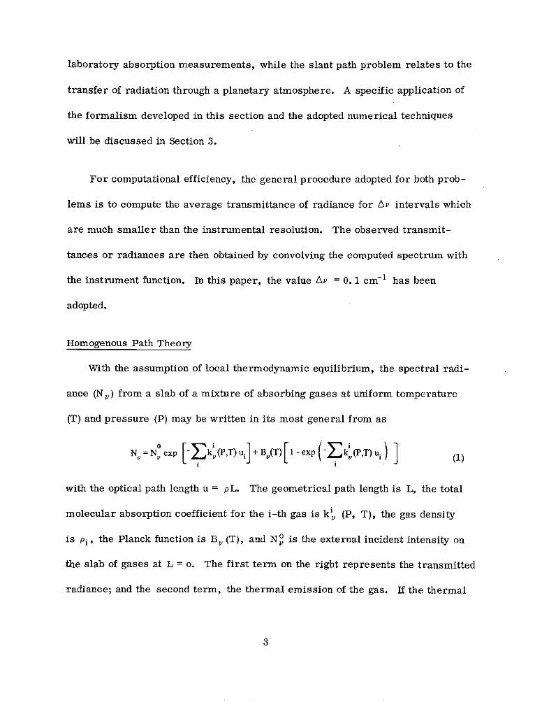
laboratory absorption measurements, while the slant path problem relates to the

transfer of radiation through a planetary atmosphere. A specific application of

the formalism developed in this section and the adopted numerical techniques

will be discussed in Section 3.

For computational efficiency, the general procedure adopted for both prob-

lems is to compute the average transmittance of radiance for Av intervals which

are much smaller than the instrumental resolution. The observed transmit-

tances or radiances are then obtained by convolving the computed spectrum with

the instrument function. In this paper, the value Av = 0. 1 cm - 1 has been

adopted.

Homogenous Path Theory

With the assumption of local thermodynamic equilibrium, the spectral radi-

ance (N,) from a slab of a mixture of absorbing gases at uniform temperature

(T) and pressure (P) may be written in its most general from as

Nv = N exp k (P,T) ui + B(T) [1 - exp k (PT) i (1)I i

with the optical path length u = pL. The geometrical path length is L, the total

molecular absorption coefficient for the i-th gas is k', (P, T), the gas density

is Pi, the Planck function is B, (T), and No is the external incident intensity on

the slab of gases at L = o. The first term on the right represents the transmitted

radiance; and the second term, the thermal emission of the gas. If the thermal

3

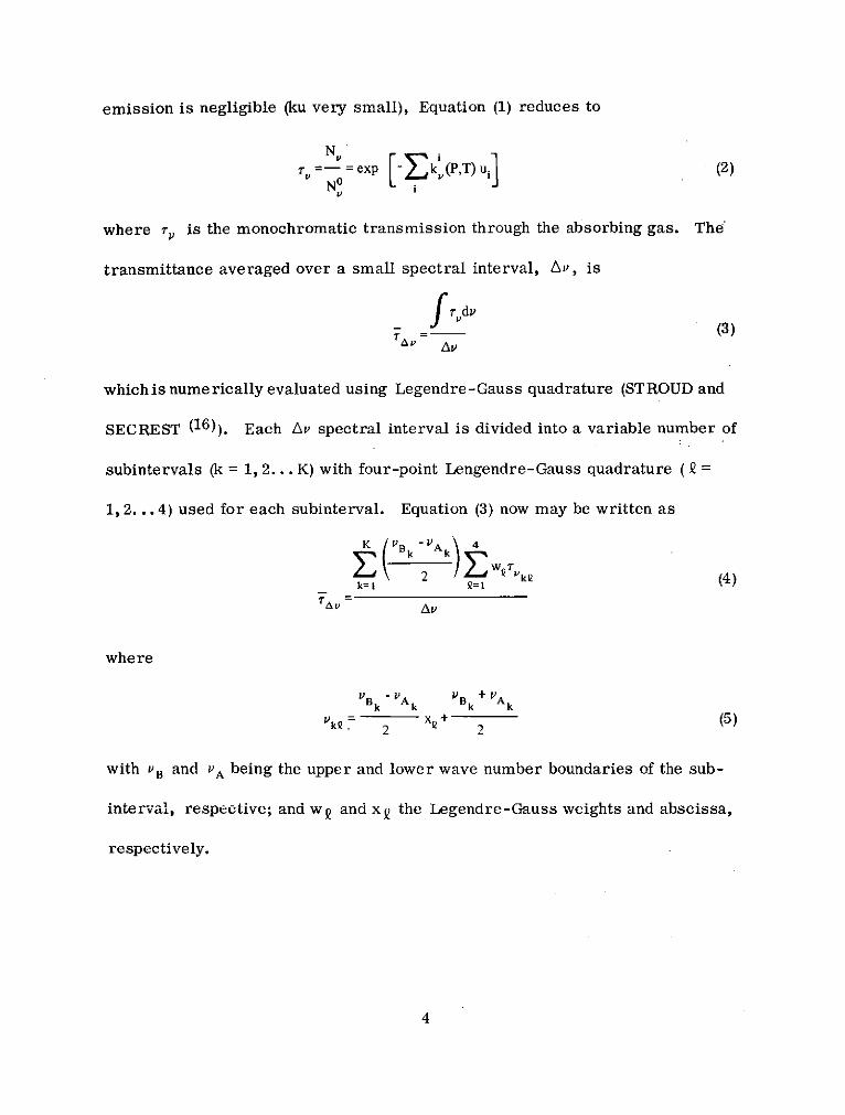
emission is negligible (ku very small), Equation (1) reduces to

NT =-x exp k (PT) ui (2)

No

where r7 is the monochromatic transmission through the absorbing gas. The

transmittance averaged over a small spectral interval, Av, is

7 dvAf(3)

which is numerically evaluated using Legendre-Gauss quadrature (STROUD and

SECREST (16)). Each Av spectral interval is divided into a variable number of

subintervals (k = 1, 2... K) with four-point Lengendre-Gauss quadrature ( =

1, 2... 4) used for each subinterval. Equation (3) now may be written as

K (vB Ak) 4

2 P k2 (4)k= 1 2= 1

where

BA B ABk Ak k Ak

Vk 7 x + (5)2 2

with vB and VA being the upper and lower wave number boundaries of the sub-

interval, respective; and wQ and x 2 the Legendre-Gauss weights and abscissa,

respectively.

4

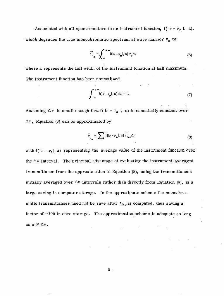
Associated with all spectrometers is an instrument function, f( Iv - v n 1, a),

which degrades the true monochromatic spectrum at wave number n to

rVn f(Iv - vnl, a) rvdv (6)

where a represents the full width of the instrument function at half maximum.

The instrument function has been normalized

f f(V - n1,a)dv 1. (7)

Assuming A v is small enough that f( Iv - vn 1, a) is essentially constant over

Av , Equation (6) can be approximated by

rV= f(lv-nl, a) AVAv (8)

with f( Iv - vn , a) representing the average value of the instrument function over

the A v interval. The principal advantage of evaluating the instrument-averaged

transmittance from the approximation in Equation (8), using the transmittances

initially averaged over Av intervals rather than directly from Equation (6), is a

large saving in computer storage. In the approximate scheme the monochro-

matic transmittances need not be save after Tra is computed, thus saving a

factor of -100 in core storage. The approximation scheme is adequate as long

as a > Av.

5

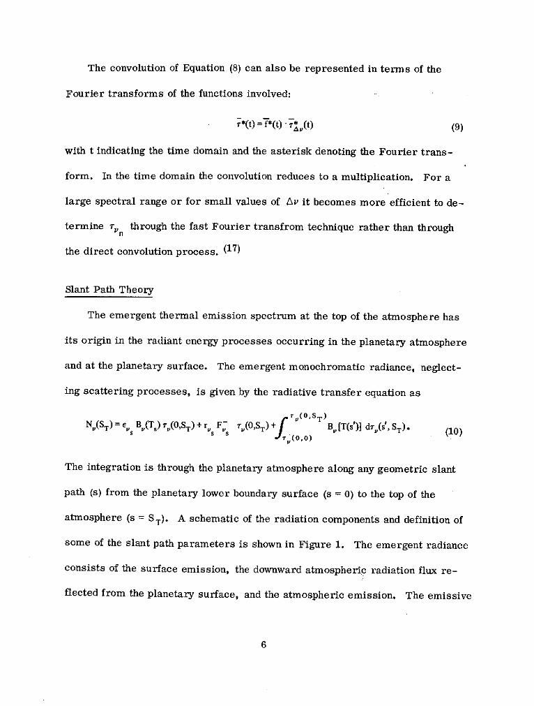
The convolution of Equation (8) can also be represented in terms of the

Fourier transforms of the functions involved:

7*(t) = f*(t) -. (t) (9)

with t indicating the time domain and the asterisk denoting the Fourier trans-

form. In the time domain the convolution reduces to a multiplication. For a

large spectral range or for small values of Av it becomes more efficient to de-

termine Trn through the fast Fourier transfrom technique rather than through

the direct convolution process. (17)

Slant Path Theory

The emergent thermal emission spectrum at the top of the atmosphere has

its origin in the radiant energy processes occurring in the planetary atmosphere

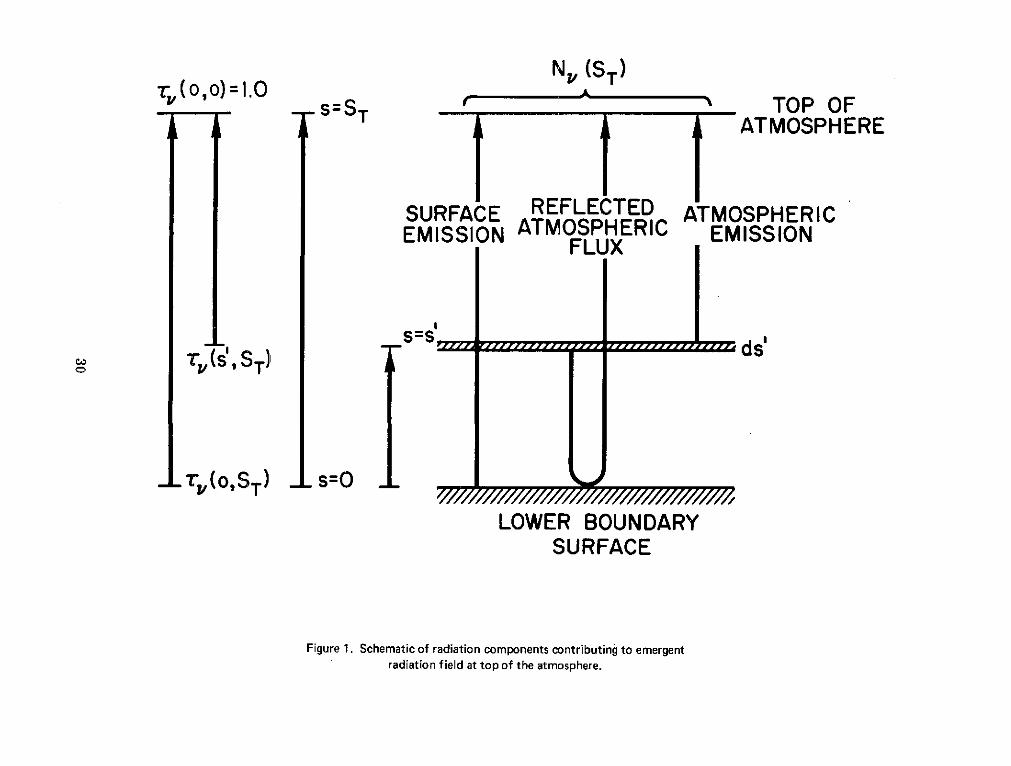
and at the planetary surface. The emergent monochromatic radiance, neglect-

ing scattering processes, is given by the radiative transfer equation as

f V(OST)

N,(ST) = e B,(T T(0,ST) + r F (0,ST) [T(s')] d(s, S). (10)

The integration is through the planetary atmosphere along any geometric slant

path (s) from the planetary lower boundary surface (s = 0) to the top of the

atmosphere (s = S T). A schematic of the radiation components and definition of

some of the slant path parameters is shown in Figure 1. The emergent radiance

consists of the surface emission, the downward atmospheric radiation flux re-

flected from the planetary surface, and the atmospheric emission. The emissive

6

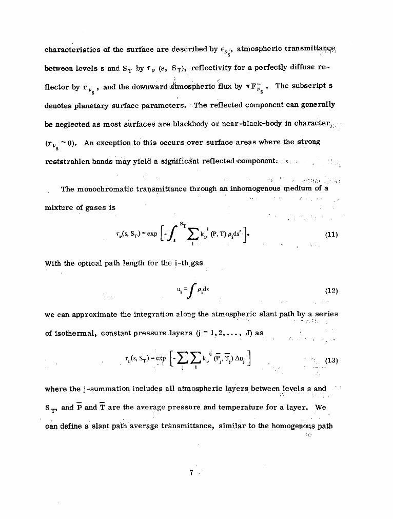
characteristics of the surface are described by e, , atmospheric transmittaiq e ,S

between levels s and ST by 7, (s, ST), reflectivity for a perfectly diffuse re-

flector by rs , and the downward atmospheric flux by irFs . The subscript ss VS

denotes planetary surface parameters. The reflected component can generally

be neglected as most surfaces are blackbody or near-black-body in character,.:

(rs ~ 0). An exception to this occurs over surface areas where -the strong

reststrahlen bands may yield a significant reflected component.

The monochromatic transmittance through an inhomogenous medium of a

mixture of gases is

v(s, ST) = exp - k, (P, T) pids' * (11)

With the optical path length for the i-th gas

Ui Pids (12)

we can approximate the integration along the atmospheric slant path by a series

of isothermal, constant pressure layers (j = 1, 2,..., J) as

7,(s, ST) exp - k (P, T)Au] (13)

where the j-summation includes all atmospheric layers between levels s and

ST, and P and T are the average pressure and temperature for a layer. We

can define a. slant path' average transmittance, similar to the homogenous path

7

average- transmittance, in terms of fourl-p.oint Legendre -Gauss quadrature ,: ,

K VBk-V 4

S2 wpkQ S'- k . (14)

The radiative transfer formulation given above describes only the general :.

approach -used to determine the emergent :spectrum for' any atmospheric slant

path, s, through a model atmosphere. A more detailed description of iethe. .: i

techniques used to relate the slant path, s, to the local vertical path, h, for a

spherical atmosphere and for the determination of the optical path lengths of

the various absorbing gases along s has been given previously (KUNDE (18)).

The emergent spectral radiance in a finite spectral interval, Av, is

NA (ST) = NV(ST)dv (15)

With Equation (10) and assuming that Av is small enough to allow the spectral

quantities to be evaluated at the midpoint of Av (denoted by v'), Equation (15)

may be expressed in terms of the average transmittance as

NA (ST) "7,v(o ' sT )

A , B1 (T 8) r,(0, S) + r, F T (0, y . () B (T(s))d (s , ST). (16)

We can numerically approximaie Equation (16) by '

NaV (ST) B ,,j, '(j ST) :n f (s' s) :NAV(ST) = & ,':B. (T4. {'( ST) Ti'iF ') + [B (s')) Ar-(s' ST)' i '(7)r: -

J

8

where the atmosphere has been divided into a series of isothermal layers with

the integral term of Equation (16) being replaced by a sum over the contributions

of all atmospheric layers. The difference in transmission across the layer is

AiA j with the layer increment taken as As' = 0.1 km. To evaluate Equation

(17) the average transmittance fA (s, ST) is precomputed for a set of atmos-

pheric levels (sp9 p = 1, 2,... N), with N being approximately 30. The N levels

are selected to yield approximately equal increments of Ar. The vertical layer

mesh usually varies from 0. 5 to 4 km with the smaller layers being concentrated

near the lower surface. The emergent spectrum for each Av = 0. 1 cm-' interval

is computed from Equation (17) for As'= 0. 1 km steps with the average trans-

mittance obtained by interpolation from the precomputed transmittance array,

TA, (sp, ST). Computing the average transmittance on a coarse vertical scale

is essential for making the direct integration calculations tractable.

In order to compare the theoretical outgoing radiances with measured radi-

ances (Nvn), we must convolve the theoretical radiances with the instrument

function, f( Iv - vn , a),

N f(lv-'vnlI,a) N(ST) dv (18)

This convolution is accomplished by a fast Fourier transform procedure in the

same manner as described for the homogenous path convolution.

9

The numerical algorithm for determining the emergent radiances incorpor-

ates the following steps:

(1) Specify atmospheric model, vertical temperature profile, vertical gas

concentration, and surface pressure

(2) Specify molecular absorbing gases and appropriate line parameters

(3) Set up vertical matrix of atmospheric temperatures, atmospheric

effective pressures, and optical path lengths for each absorbing gas

for each atmospheric layer

(4) Determine the average transmittance for a 0. 1 cm - 1 interval for J

atmospheric levels from Equations (13) and (14)

(5) Determine the emergent radiance for each 0. 1 cm- 1 interval from

Equation (17) across the spectral region of interest

(6) Determine the emergent radiance averaged over the instrument function

as specified in Equation (18), for comparison to the observed spectrum.

This algorithm has been programmed entirely in FORTRAN IV for an IBM 360

operating system.

3. MONOCHROMATIC MOLECULAR ABSORPTION COEFFICIENT

FORMULATION

In this section we will describe the determination of the monochromatic

molecular absorption coefficient at the Vk2 wave number mesh points necessary

for the monochromatic transmittances.

10

A molecular absorption line can be described by four parameters: line

position (Vo), integrated line intensity (S), relative line shape (b), and line half-

width (a). The absorption coefficient for a single line is

2 = S b(v - vo , a) (19)

where the relative line shape b(v - v, a) depends on the type of line-broadening

mechanism considered.

The two line shapes of importance in the terrestrial atmosphere are the

thermal Doppler

\/n -(V -VD) Rn2b(v - vo, aD) = - exp 1 (20)

and the collision-broadened Lorentz

ac 1b(v - vo , ac) = - 0)2 + C2 (21)

n7r (V - )+

with aD and ac being the Doppler and collisional line half-widths, respectively.

The mixed Lorentz-Doppler line shape is

n2 1b(a, u) = - H(a, u) (22)

where a = (aC/aD) 2n2 and u = [ (v - Vo)/aD i] n 2. The function H(a, u) has

been evaluated following a numerical scheme of YOUNG (19). Kinetic theory

predicts the temperature and pressure dependence of the collisional half-width

11

to be

P/T\

ac(PT)= ac(P, Tr) P (23)

with y= 0. 5. The subscripts r refer to reference conditions. For a mixture of

gases, the pressure P is usually converted to an effective pressure, (P ),

Pe = P + (B - 1) pa (24)

to correct for the influence of self-broadening on the line half-width. The partial

pressure of the absorbing gas is Pa and B is the self-broadening coefficient.

The collisional line half-width now may be written as

P pT \ T

ac(Pe ,T)= ac(Pr, Tr) (25)

The molecular absorption coefficient at a specific wave number is the sum-

mation of the contribution from each of the individual molecular absorption lines,

k (P,T) vm(P,T) = Sm(T) b(v- vo m, , (P,T)) (26)

m m

For planetary atmospheres the monochromatic absorption coefficient varies by

orders of magnitude on a scale of 1/1000 cm - 1 for wave numbers near the line

center, while in the line wings the absorption coefficient changes much more

gradually. To retain a high degree of accuracy in the transmittance computa-

tions, the rapidly varying behavior of the absorption coefficient requires a wave

number mesh spacing of the order 1/1000 cm - 1 near the line center, while

12

1/10 cm - 1 will suffice in the line wings. The method used to evaluate Equation

(26) is patterned after the numerical technique developed by DRAYSON (8).

Basic to this procedure are a division of each line into direct and wing contri-

butions and the establishment of a variable wave number mesh for the evaluation

of k, (P, T).

The direct contribution includes all wave numbers within a distance 6 of the

line center, and the wing contribution includes all wave numbers equal to or

greater than 6,

D W

VV + k (27)

where 6 has been chosen as 3. 5 cm - 1 . The total molecular absorption coeffi-

cient now becomes

k (Pe, T) = (Pe, T) + 2(PT) (28)m m

which can be rewrittenD W

kv(Pe,T)= k (PT) + k (PeT) (29)

with

w wkv (Pe, T) = WmPe, T) IAvI>

D (PT)= D (30)kv (P, T)= EPe, T). IAvl <

13

The technique of separating each line into direct and wing contributions has the

advantage that one need consider only lines in the interval v - 5 to v + 5, rather

than all lines, for computing the direct contribution, thus insuring a considerable

reduction in the amount of computer time required. A second advantage is that

the wing contribution may be easily adjusted for empirical fitting to observed

spectra in spectral regions where the theoretical treatment is not adequate. An

example of this will be discussed later for the water vapor continuum in the 500

and 1000 cm - 1 windows.

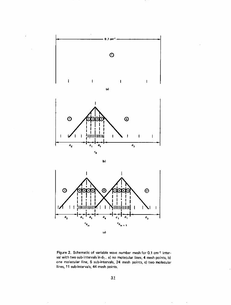
The determination of the wave number mesh for the direct contribution will

be described briefly with the aid of Figure 2. Cases where no line, one line,

and two lines fall within the Av = 0.1 cm - 1 interval are shown in Figure 2(a),

2(b), and 2(c), respectively. The circled numbers indicate the subinterval

number; the dashed lines, the subinterval boundaries; and the short lines near

the bottom of each figure indicate schematically the wave number mesh. The

wave number scale is distorted near the line centers for clarity of presentation.

The distance d i from the line center is subdivided into subintervals, each con-

taining four mesh points whose positions within the subinterval are specified

by the Legendre-Gauss quadrature abscissa points. The distance d 1 is usually

chosen as 0.01 cm - 1 and the number of subintervals in d i is a variable in the

range of from one to five with the higher number of subintervals yielding more

accurate transmittance values. The number of subintervals is usually taken as

14

two, which allows the transmittances to be computed with a numerical accuracy

of two to three significant figures, an accuracy which is sufficient for most

applications. After the subintervals are established near the line center, the

remaining sections of the interval, d 2 and d 3 in Figure 2(b), d 2, d 3 , and d 4 in

Figure 2(c), are each assigned as one subinterval. For more than two lines in

a 0. 1 cm - l interval the division scheme of Figure 2(c) is applied repeatedly.

Without lines in the 0. 1 cm - 1 interval, the four-point Legendre-Gauss quad-

rature is applied to the entire 0. 1 cm - 1 interval. The scale of the variable

wave number mesh is thus of the order 0. 001-0. 01 cm-1.

The mixed Doppler-Lorentz line shape is used in the direct contribution if

the total pressure is less than 100 mb and the distance from the line center is

less than 0. 2 cm - 1 . The Lorentz line shape is used for the remaining direct

contribution.

The collisional line shape is applicable for the wing contribution which,

from Equations (19), (21), and (30) and using the condition A, > ac (Pr, Tr)

W O ek (Pe, T) = k (T) P (31)

r

with

Sm (T) a (PrTr) T

m n (V-v o ) 2 (32)

15

The function k ° (T) changes slowly with respect to wave number and thus may

be precomputed at a coarser wave number grid (- 0. 5 cm-' ) than required for

the direct contribution with intermediate values obtained by interpolation.

From Equations (19), (29), and (31), the total monochromatic absorption

coefficient necessary for determining the monochromatic transmittance for the

i-th gas and j-th layer (see Equation 13) is

U -- - - O e

kvki , Tj)= mS (Ti)bm(Pe, T i ) + kl (T)Pr (33)

The molecular line parameters for the evaluation of Equation (33) are stored on

magnetic tape, ordered by ascending wave number, with the parameters o%,

Icode, ac, y, S(175 K), S(200 K), ... , S(300 K) preserved for each line and

with Icode identifying the species of gas. The present atlas contains -6000

H 20 lines, - 5000 03 lines, and -10, 000 lines of CO 2 in the 200 to 2000 cm - 1

range. The sources of these line parameters and the modifications for em-

pirical line shapes are the subject of the next section.

4. SOURCES FOR MOLECULAR TRANSMITTANCE PARAMETERS

The molecular line parameters for carbon dioxide, water vapor, and ozone

were collected from a variety of sources. The molecular parameters for CO 2

are generated in the following manner. The line positions and strengths have

been determined for 68 bands of C12 0216, using standard spectroscopic formu-

lation for a linear molecule, from band center positions, energy levels,

16

rotational constants, and band strengths provided by BENEDICT (20). The only

exception is that the band intensities of DRAYSON (21) are used if significant

differences exist. The band parameters for the stronger C 2 0216 bands are

listed in Table 1. Also included in the computations are 70 isotopic bands of

carbon dioxide. The strengths of these bands relative to the corresponding

bands of C 1 2 0216 are taken to be the same as the abundance of the species

relative to C12 0216. The relative abundances are calculated from the ter-

restrial abundances of the isotopes of carbon and oxygen.

The self- and nitrogen-broadened line half-widths for carbon dioxide as a

function of rotational quantum number were obtained from YAMAMOTO et al. (22),

and were assumed to be valid for all vibrational bands.

The CO 2 continuum is substantially sub-Lorentzian in the 1000 cm - 1 re-

gion. BIGNE LL et al. (23) have reported experimental work from which they

concluded the absorption by CO 2 outside the range from 560 to 790 cm - 1 is

negligible. WINTERS (24), following suggestions by BENEDICT, found that an

exponential modification of the Lorentz line shape beyond some minimum dis-

tance from the line center improved the agreement of calculated and experi-

mental absorptance for CO 2 in the 2400 cm - 1 region. Recently, BIRNBAUM (25)

has developed a theoretical basis for a line shape which is Lorentzian near the

line center and exponential sufficiently far from the line center. The point at

which the shape becomes exponential depends on the duration of collision.

17

BURCH (26) has found that the wings of nitrogen-broadened CO 2 lines absorb

only about 1 percent as much in the 780-900 cm-' regions as if they had the

Lorentz shape. To fit the experimental CO 2 continuum we have assumed an

exponential modification of the Lorentz line shape

b = bLorentz 0 mm(34)

b = bLorentz exp [a I IV -P in o > Vmin

beyond min = 3. 5 cm-1 from the line center for all CO 2 lines in the 500 to 800

cm - 1 region. The parameters a and b have been calculated using WINTERS'

et al. (24) values a = 0. 08 and b = 0. 8 as starting values and running a mesh of

a's and b's to find the parameters which reproduce the experimental continuum

absorption. The best fit is obtained with a = 1. 4 and b = 0. 25. The above ex-

ponential correction was also used for the CO 2 continuum in the 500 cm - 1 window

region. A fit to the self-broadened CO 2 continuum of BURCH (26) yields values

of a and b approximately the same as the nitrogen-broadened continuum values.

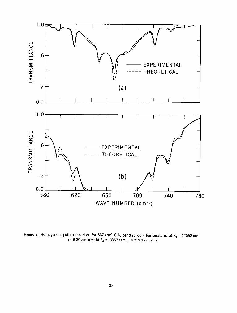
The accuracy of the theoretical calculations was checked by computing the

transmission for various homogenous path pressures and optical masses and

comparing with published experimental spectra (BURCH et al. (27)). Two of

these cases are shown in Figure 3, with the theoretical transmission being

computed with a triangular instrument function of 4 cm - 1 full width at half-

maximum. The solid line represents the measurement, and the dashed line,

the calculation. The agreement is better than 10 percent for both cases. The

18

errors in the strong Q-branch regions are enhanced by imprecise knowledge of

the true instrument function and do not reflect a major discrepancy between the

theoretical and experimental transmittances. However, the theoretical com-

putations need improvement for the pressure-broadened line shape within 5 cm - 1

from the line center. The investigations of BURCH et al. (28) have indicated

significant deviations from the Lorentz shape for self-broadened CO 2 lines in

the 2400, 3800, and 7000 cm- 1 regions. Experimental investigations are needed

to determine the deviation for N 2-CO 2 and CO2-CO 2 collisions for the 667 cm - 1

band.

The line data used for water vapor are taken from BENEDICT and

KAPLAN (29) for the pure rotational lines and from BENEDICT and CALFEE (30)

for the 1595 cm- 1 band.

One of the most difficult problems to treat in atmospheric transmission

models is the water vapor continuum regions. The difficulties arise because of

uncertainties in the effect of aerosols, in knowledge of molecular line shapes in

the far wings of lines, and in knowledge of the physical mechanisms responsible

for the water vapor absorption. Water vapor continuum absorption in the 500

cm - 1 and 1000 cm - 1 windows was discussed in the Nimbus 3 IRIS paper

(CONRATH et al. (31)). The water vapor continuum absorption coefficients

adopted for the Nimbus 3 investigation gave good agreement in the 1000 cm - 1

window, but overestimated the absorption in the 500 cm -1 window.

19

Since the publication of Reference 31, a number of pertinent laboratory and

free atmosphere investigations concerning water vapor continuum absorption

have been published. Laboratory measurements by BIGNELL (32) and

BURCH (26) indicate the water vapor continuum absorption in the 500 cm - 1 and

1000 cm- 1 regions consists of two components, one proportional to the total

pressure and the other to the water-vapor partial pressure:

k(P, pH2, T) = k i (T) P + k2 (T) pH2 0 (35)

BIGNELL (32) has also reinterpreted, in a semiquantitative sense, previous

atmospheric and laboratory measurements in these spectral regions and con-

cludes that the previous work in general substantiates the two-component

mechanism. Recent interpretations of atmospheric measurements by

PLATT, (33, 34) WARK, (35) and HOUGHTON and LEE (36) have further veri-

fied the Bignell and Burch results.

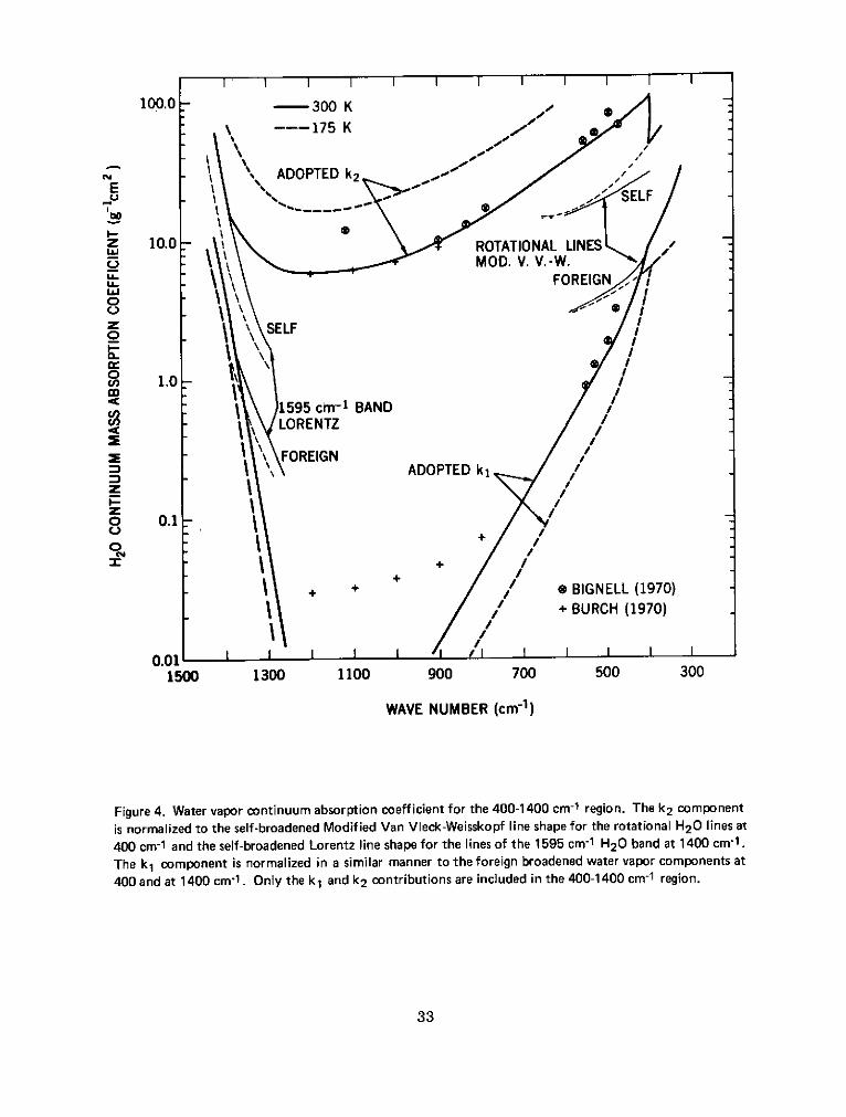
The two-component continuum has been incorporated in the transmittance

model; the adopted k1 and k 2 values are illustrated in Figure 4. Laboratory

values of k , in the 1000 cm - 1 regions are not available due to experimental

difficulties. The laboratory values of Burch for this region shown in Figure 4

represent only the upper limits to k . The investigations of WARK (35) and

HOUGHTON and LEE (36) gave satisfactory results with the k 1 value in the

1000 cm - 1 window essentially zero. Based on their success, we have forced

k to approximately zero by extrapolation of the measured k1 component from

20

the 500 cm - 1 window region and of the computed Lorentz foreign-broadened

wing component of the 1595 cm - 1 H 20 band. The k 1 and k 2 components at 175 K

were scaled from the 300 K values using the temperature dependence of Bignell.

Also shown in Figure 4 is the wing contribution of the rotational water-vapor

lines using the modified Van Vleck-Weisskopf (M-VVW) line shape described

by FARMER (37). All self-broadened components have been computed for a

self-broadening coefficient of 6. 3. As illustrated in Reference 31, no theoret-

ical line shape is adequate for the 500 cm - 1 and 1000 cm -1 window regions..

However, M-VVW line shape gives fair agreement with the measurements of

PALMER (38) in the 250-350 cm - 1 range and, for continuity, the adopted k, and

k 2 components are normalized to the M-VVW at 400 cm -1 . The Lorentz line

shape is used for the 1595 cm - 1 H 2 0 band with the normalization to k, and k2 oc-

curring at 1400 cm - 1 . The normalization results in slight discontinuities,

which, however, create no problems in practice. The water vapor continuum

absorption in the 400 to 1400 cm - 1 range thus is based on laboratory data com-

puted from Equation (35) with the k1 and k 2 values determined numerically.

For water vapor in this region, Equation (35) replaces the term k' (Pe, T) of

Equation (29).

The adopted water vapor continuum absorption coefficients are employed

in the transmittance model in an empirical sense, to be used as part of a work-

ing model until more knowledge is acquired of the opacity sources and their

21

governing physical mechanisms. While the empirical model may still need

considerable adjustment with regard to the actual numerical magnitudes of k 1

and k 2, it is felt that the two-component concept, especially the PH 20 term, is

an important step forward in coping with water vapor continuum transmittance

problems.

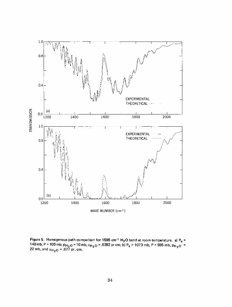
Homogenous path comparisons for the 1595 cm - 1 H 20 band are shown in

Figure 5. The experimental data of BURCH et al. (27) varied in spectral resolu-

tion from -- 5 cm - 1 at 1200 cm - 1 to -20 cm -' at 2000 cm- ' . Thus the R branch

side of the band does not exhibit much line structure. The agreement in the P

and R branches is better than 5 percent, with the theoretical transmittances

being slightly too transparent in the continuum.

The first-generation ozone line parameters was not very satisfactory, as

evidenced in the radiance comparisons of Reference 31. A second-generation

set of ozone lines is now available; the main improvement is the inclusion of

numerous upper-state bands. This line set seems to be more satisfactory

based on comparisons to balloon flight measurements by GOLDMAN et al. (39)

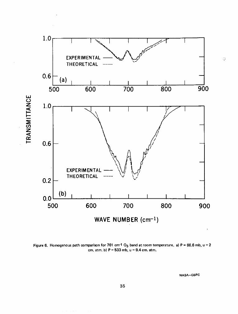
and to laboratory data by AIDA (40). Included in this line set is the v2 band at

701. 4 cm - 1 , a band which is of importance to atmospheric temperature inver-

sions in the 667 cm -1 CO 2 band region. Theoretical calculations for this band

are compared to the laboratory spectra of McCAA and SHAW (41) in Figure 6.

The number of lines considered for the v2 band was 2158, with a collisional

22

half-width of 0. 07 cm -1 at 296 K and a Lorentz line-shape. Self-broadening

effects were assumed to be unimportant. The general agreement is approxi-

mately 5 to 10 percent which is satisfactory for initial applications to the tem-

perature inversion problem. Absorption by these lines is demonstrated for. a

slant path in the paper on application to the Nimbus 4 IRIS spectra (KUNDE (15)).

5. CONCLUDING REMARKS

A direct integration transmittance model has been developed for

interpretation of spectra of intermediate to high spectral resolution recorded

in the laboratory or in the atmosphere. This procedure, though time-consuming

on present digital computers, avoids limitations and approximations necessary

when employing empirical representations and band models for computation of

molecular absorption. The main advantages of the direct integration technique

are the ability to attain high spectral resolution and to easily vary this resolu-

tion; to facilitate different types of line shapes readily, including mixed line

shapes; to handle line wing effects; to cope with temperature, pressure, and gas

concentration variations, and to avoid assumptions necessary to reduce a slant

path absorption to the equivalent homogenous path absorption. The central con-

cepts for making the direct integration a tractable problem are the variable wave

number mesh and the division of each line into direct and wing contributions. As

the numerical procedures are essentially exact, the accuracy of the predicted

transmittances is limited by the accuracy of the input molecular parameters.

23

As a consistency check on the input line parameters and the transmittance

model, theoretical predictions have been compared to existing laboratory data

for several representative homogenous path cases. The comparisons gave

transmittance disagreements of 5 to 10 percent, a number which is probably in-

dicative of the absolute accuracy of present state-of-the-art molecular

transmittances.

The accuracy of the slant path model and the predicted transmittances has

been assessed by comparison to Nimbus 4 IRIS data, and Mariner 9 IRIS data,

with both applications yielding agreements of 5 to 10 percent in emergent

radiances through the 200 to 2000 cm -1 region. The model is presently being

tested further against high spectral resolution terrestrial transmittance spectra

(- 0. 2 cm -1 ) and downward sky emission spectra in the 450 to 1400 cm -1 re-

gion obtained from McDonald and Mauna Kea Observatory.

ACKNOWLEDGMENTS

We would like to thank Dr. W. S. Benedict, University of Maryland, and

Dr. S. R. Drayson, University of Michigan, for providing the CO 2 energy levels,

rotational constants, andband intensities. We are also indebted to Dr. Drayson

for numerous discussions concerning the direct integration technique and to

Dr. R. Hanel for suggestions in improving the manuscript. Programming the

convolution of the monochromatic spectrum with the instrument function using

fast Fourier transform techniques was accomplished by L. Herath, Goddard

Space Flight Center.24

REFERENCES

1. R. A. Hanel, B. J. Conrath, V. G. Kunde, C. Prabhakara, I. Revah,

V. V. Salomonson, and G. Wolford, JGR, 77, 2629 (1972).

2. J. Connes, P. Connes, and J. P. Maillard, "Atlas des spectres dans le

proche infrarouge de Venus, Mars, Jupiter et Saturne, " Centre National

de la Recherche Scientifique, Paris (1969).

3. R. A. Hanel, V. G. Kunde, T. Meilleur, and G. Stambach, Planetary

Atmospheres. C. Sagan, ed., Reidel (1971).

4. D. M. Rank, private communication (1972).

5. R. A. Hanel, B. Conrath, W. Hovis, V. Kunde, P. Lowman, W.

Maguire, J. Pearl, J. Pirraglia, C. Prabhakara, B. Schlachman, G.

Levin, P. Straat, and T. Burke, Icarus, 17, 423 (1972).

6. P. Connes, J. Connes, R. Bouigue, M. Querci, J. Chauville, and F.

Querci, Annales d'Astrophysique, Tome 31, Fascicule 5 (1968).

7. T. R. Geballe, E. R. Wollman, and D. M. Rank, Ap. J. Letters, 177,

L27 (1972).

8. S. R. Drayson, Appl . Opt., 5, 385 (1966).

9. T. G. Kyle, JQSRT, 9, 1477 (1969).

25

10. V. G. Kunde, Ap. J., 153, 435 (1968).

11. J. R. Auman, Ap. J. Suppl., 14, 171 (1967).

12. F. Querci, M. Querci, and V. G. Kunde, Astron. & Astrophys., 15,

256 (1971).

13. R. F. Calfee, JQSRT, 6, 221 (1966).

14. J. O. Arnold, E. E. Whiting, and G. C. Lyle, JQSRT, 9, 775 (1969).

15. V. G. Kunde, B. J. Conrath, R. A. Hanel, W. C. Maguire, C.

Prabhakara, and V. V. Salomonson, JGR, to be published (1973).

16. A. H. Stroud and D. Secrest, "Gaussian Quadrature Formulas,"

Prentice-Hall, Inc., Englewood Cliffs, N. J. (1966).

17. J. W. Brault and 0. R. White, Astron. & Astrophys., 13, 169 (1971).

18. V. G. Kunde, NASA TN D-4045, August (1967).

19. C. Young, JQSRT, 5, 549 (1965).

20. W. S. Benedict, private communication (1971).

21. S. R. Drayson, "Proceedings of Conference on Atmospheric Radiation, "

Colorado State University, Fort Collins, Colorado, August 7-9, (1972).

22. G. Yamamoto, M. Tanaka, and T. Aoki, JQSRT, 9, 371 (1969).

23. K. Bignell, F. Saiedy, and P. A. Sheppard, JOSA, 53, 466 (1963).

24. B. H. Winters, S. Silverman, and W. S. Benedict, JQSRT, 4, 527

(1964).

26

25. G. Birnbaum, "The Shape of Collision Broadened Lines Near Resonance

and in the Far Wings, " to be published (1973).

26. D. E. Burch, Philco-Ford Corporation Aeronautronic Division Publica-

tion U-4784, January 31, (1970).

27. D. E. Burch, D. Gryvnak, E. B. Singleton, W. L. France, and D.

Williams, AFCRL-62-698, July (1962).

28. D. E. Burch, D. A. Gryvnak, R. R.. Patty, and C. E. Bartky, JOSA,

59, 267 (1969).

29. W. S. Benedict and L. D. Kaplan, private communication (1967).

30. W. S. Benedict and R F. Calfee, ESSA Prof. Paper 2, June (1967).

31. B. J. Conrath, R. A. Hanel, V. G. Kunde, and C. Prabhakara, JGR,

75, 5831 (1970).

32. K. J. Bignell, QJRMS, 96, 390 (1970).

33. C. M. R. Platt, NATURE, 235, 29 (1972).

34. C. M. R. Platt, JGR, 77, 1597 (1972).

35. D. Q. Wark, "Proceedings of International Radiation Symposium, "

Sendai, Japan, May 26 - June 2, (1972).

36. J. T. Houghton and A. C. L. Lee, NATURE, 238, 117 (1972).

37. C. B. Farmer, E. M. I. Ltd. Rep. DMP 2780, Hayes, Middlesex,

England, April (1967).

27

38. C. H. Palmer, JOSA, 47, 1024 (1957).

39. A. Goldman, T. G. Kyle, D. G. Murcray, F. H. Murcray, and W. J.

Williams, Appl. Opt., 9, 565 (1970).

40. Masaru Aida, "Proceedings of International Radiation Symposium,"

Sendai, Japan, May 26 - June 2, (1972).

41. D. J. McCaa and J. H. Shaw, AFCRL-67-0237, February (1967).

28

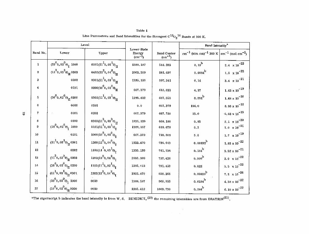
Table 1

Line Parameters and Band Intensities for the Strongest C120216 Bands at 300 K.

Level Band Intensity*Lower State

Band No. Lower Upper Energy Band Center cm - 1 (atm cm)- 1 300 K cm - 1 (mol cm - 2)(cm-1) (cm- I )

1 (1000,0200)I 1000 0301(1110,0310)i 1388.187 544.283 0 . 1 0b 2.4 x 10-22

2 (1130,0330)H 0303 0402(1220, 0420) 2003.309 581.697 0. 0 0 84 b 1.5 x 10-22

3 0202 0301(1110,03 10) 1335. 129 597.341 0.14 3.4 x 10 - 2 1

4 0101 0200(1000,0200)II 667.379 618.033 4.27 1.43 x 10-19

5 (1000,0200)11 0200 0301(1110, 0310)1 1285. 412 647. 058 0. 5 9 1b 1.48 x 10-20

6 0000 0101 0.0 667. 379 194.0 8. 93 x 10 - 1 8

7 0101 0202 667.379 667.750 15.0 -5.03 x 10 - 1 9

8 0202 0303(1130, 0330)H 1335.129 668. 180 0.85 2.1 x 10- 20

9 (1000,0200)1 1000 1101(11 10,0310)1 1388.187 688. 678 0.3 7.0 x 10

10 0101 1000(1000,0200)i 667.379 720.808 5.0 1.7 x 10- 19

11 (11 10,03 10) 0301 1200(12 00, 04 00) 1932.470 738. 643 0.00832 1.53 x 10- 2 2

12 0202 1101(11 10,03 10) 1335. 139 741. 736 0. 144b 3.52 x 10-2 1

13 (1130,03 30) 0303 1202(12 20,04 20) 2003.309 757.426 0.009b 2.0 x 10-22

14 (1000,0200) 0200 1101(1110,0310)I 1285.412 791.453 0.022 5.5 x 10-22

15 (1110,0310) 0301 1202(1220,0420)1 1932.470 828. 265 0. 000 39b 7.2 x 10-24

0 0 b -22

16 (1000,0200) 1000 0010 1388.187 960.955 0.0184 b 4.38 x 10-22

17 (10 00,0200)I 0200 0010 1285.412 1063.730 0.244b 6.10 x 10-22

*The superscript b indicates the band intensity is from W. S. BENEDICT, (20) the remaining intensities are from DRAYSON (2 1 ) .

N, (ST)-S(o). S _ TOP OF

ST -t ATMOSPHERE

SURFACE REFLECTED ATMOSPHERICEMISSION ATMOSPHERIC EMISSIONFLUX

S=S_ ds'T (S, S T)

TV (o,ST ) s=O

LOWER BOUNDARYSURFACE

Figure 1. Schematic of radiation components contributing to emergentradiation field at top of the atmosphere.

0.1 CnW

0 3 4 5

d I iI I!

d2. d d d

V0

(b)

0 2345 0 78910

d ,2 d,- dr

d 4 dI di I d3

VOm m + 1

(c)

Figure 2. Schematic of variable wave number mesh for 0.1 cm-1 inter-val with two sub-intervals in d1 . a) no molecular lines, 4 mesh points, b)one molecular line, 6 sub-intervals, 24 mesh points, c) two molecularlines, 11 sub-intervals, 44 mesh points.

31

1.0

C/z -,

S- EXPERIMENTALz ----- THEORETICAL

i-

.2 (a)

0.0 I I I I I

1.0

z- .6 EXPERIMENTAL

S----- THEORETICALz -

.2 - (b) -

0.0580 620 660 700 740 780

WAVE NUMBER (cm- 1)

Figure 3. Homogenous path comparison for 667 cm- 1 CO02 band at room temperature: a) Pe = 02053 atm,u = 6.30 cm atm; b) Pe = .0857 atm, u = 212.1 cm atm.

32

I I I I I I I I I I I I

100.0 - 300 K

--- 175 K

N-M \ ADOPTED k2E ®u I' SELF

_\. MOD. V. V.-W.LFOREIGN iI-I0

r- n\ 1

o I

1595 cm lrr BANDLORENTZ

E /:s \ FOREIGN

ADOPTED kl /

o 0.1

+ /+ + / * BIGNELL (1970)

/ + BURCH (1970)\/

0.01 /

1500 1300 1100 900 700 500 300

WAVE NUMBER (cm- 1 )

Figure 4. Water vapor continuum absorption coefficient for the 400-1400 cm-1 region. The k2 componentis normalized to the self-broadened Modified Van Vleck-Weisskopf line shape for the rotational H20 lines at400 cm-1 and the self-broadened Lorentz line shape for the lines of the 1595 cm-1 H2 0 band at 1400 cm-1 .

The k1 component is normalized in a similar manner to the foreign broadened water vapor components at

400 and at 1400 cm- 1. Only the k1 and k2 contributions are included in the 400-1400 cm-1 region.

33

1 .0 I I I I

0.8 -

0.4 -

EXPERIMENTAL _THEORETICAL -

Z (a)0.0 I I I I

_ 1200 1400 1600 1800 2000

< 1.0

EXPERIMENTAL ---THEORETICAL -0.8-

0.4

J" i 1

0.0 (b)1200 1400 1600 1800 2000

WAVE NUMBER (cm-1 )

Figure 5. Homogenous path comparison for 1595 cm- 1 H2 0 band at room temperature. a) Pe =140 mb, P = 100 mb, pH 2 0 = 10 mb, uH20 =.0352 pr cm; b) Pe = 1073 mb, P= 985 mb, PH2022 mb, and uH2 0 = .077 pr. cm.

34

1.0 I I r

EXPERIMENTAL -'THEORETICAL

0.6 (a) I

500 600 700 800 900wz 1.0

z

0.6 -

EXPERIMENTAL -THEORETICAL ---- \

0.2

0.0 (b) I I I I I

500 600 700 800 900

WAVE NUMBER (cm- 1)

Figure 6. Homogenous path comparison for 701 cm-1 03 band at room temperature. a) P = 66.6 mb, u = 2cm. atm. b) P = 533 mb, u = 9.4 cm. atm.

NASA-GSFC

35