DirectEstimationofFiringRatesfromCalciumImagingData

EladGanmor1,MichaelKrumin2,LuigiF.Rossi2,MatteoCarandini2&EeroP.Simoncelli1,3

1. CenterforNeuralScience,NewYorkUniversity

2. UCLInstituteofOphthalmology,UniversityCollegeLondon

3. HowardHughesMedicalInstitute,NewYorkUniversity

Correspondingauthor:

EladGanmor NewYorkUniversity CenterforNeuralScience 4WashingtonPlace,Room1027 NewYork,NY10003 (212)992-8752 elad.ganmor@gmail.comKeywords:calciumimaging,deconvolution,tuningcurves,rateestimation

2

AbstractTwo-photon imagingof calcium indicators allows simultaneous recordingof responsesof

hundredsofneuronsoverhoursandevendays,butprovidesarelativelyindirectmeasure

oftheirspikingactivity.Existing“deconvolution”algorithmsattempttorecoverspikesfrom

observed imagingdata,whicharethencommonlysubjectedtothesameanalysesthatare

appliedtoelectrophysiologicallyrecordedspikes(e.g.,estimationofaveragefiringrates,or

tuningcurves).Hereweshow,however,thatinthepresenceofnoisethisapproachisoften

heavilybiased.Weproposeanalternativeanalysisthataimstoestimatetheunderlyingrate

directly, by integrating over the unobserved spikes instead of committing to a single

estimateof the spike train.This approach canbeused to estimateaverage firing ratesor

tuningcurvesdirectlyfromtheimagingdata,andissufficientlyflexibletoincorporateprior

knowledgeabouttuningstructure.Weshowthatdirectlyestimatedratesaremoreaccurate

than those obtained from averaging of spikes estimated through deconvolution, both on

simulateddataandonimagingdataacquiredinmousevisualcortex.

3

IntroductionNeurons convey information using spikes. For example, sensory neurons emit different

numbers of spikes with different timings in response to different stimuli. Yet these

responsesareoftendescribedas ‘noisy’sincetheresponsesto identicalstimulivary from

one trial to the next even when external factors are carefully controlled. Therefore, it is

commontosummarizeneuralresponses in termsofaveragespikecountsacrossmultiple

trials,acknowledgingthestochasticnatureofspikegeneration.

Estimating firingrates isaubiquitous formofanalysis throughoutneurophysiology.Well-

known examples include spike count histograms and tuning curves. The spike count

histogramrepresentstheaverageresponseoverafixedtimeintervalacrossmanyrepeats

ofthesameexperimentalcondition,relativetosomestimulusorbehavioralresponse,while

the tuning curve is a measure of the firing rate under different experimental conditions

(typically, stimulioractions thatvaryalongsomeparametricaxis).Estimating rates from

spikes thus requires combining spike counts across repeated measurements, and is

relatively straightforward when spikes are recorded directly, as is the case in

electrophysiologyexperiments.

Imaging techniques provide an appealing means of measuring neural activity across

populations. Two-photon imaging of calcium indicators, in particular, allows one to

measure up to thousands of neurons simultaneously at single-cell or even sub-cellular

resolution. Moreover, imaging techniques are readily combined with genetic and opto-

geneticmethodstorecordandstimulatespecificcelltypes.Butincomparisontoelectrical

recordings,calciumimagingprovidesalessdirectmeasureofspikingactivity:theacquired

image represents the intensity of a fluorescence signal that depends on the intracellular

calcium level, which, in turn, is driven by the spiking activity. Consequently, it is not

straightforward to estimate firing rates from calcium imaging data -- simple averaging

acrosstrialsisnotsufficient.

Themost intuitivemethodofobtainingspikerates fromimagingdata is to invert thetwo

stepsoftheobservationprocess:estimatingthespiketrainsfromthefluorescence,andthen

averaging the estimated spike counts to infer the rate. Estimating spike trains from

fluorescence is commonly referred to as deconvolution, reflecting an assumption that

intracellularcalciumlevelsaretheoutcomeofaconvolutionofthespiketrainwithaknown

4

temporal filter - deconvolution seeks to undo this process. Several algorithms have been

proposedtoperformthisdeconvolutionstep(Vogelsteinetal.2010;Oñativia,Schultz,and

Dragotti2013;Dyeretal.2010;Greweetal.2010),andhavebeensuccessfullyappliedto

estimatespikeratesandtuningcurvesfromimagingdata(SmithandHäusser2010;Koet

al.2013).

Despite the successes of deconvolution methods, it is important to recognize that spike

counts estimated from thedeconvolutionprocess are only approximate.Moreover, aswe

show, errors canbe substantial, andmore importantlymaydepend systematicallyon the

firing rate. As such, these errors are not reduced as onewould expect by averaging over

repeatedtrials.Furthermore,deconvolutionmethodsdonottakeintoaccountthestructure

oftheexperiment(specifically,thetimingandsequenceofstimuliorbehavioralresponses),

although these factors may have a significant impact on spiking activity. And even if

subsequent stages of analysis attempt to incorporate such experimental details, the

decisionsmadeduring thedeconvolutionstagetypicallycannotbeundone:missedspikes

are irretrievably lost and falsely detected spikes cannot be distinguished from their

correctlyidentifiedneighbors.

Here,weintroduceanalternativeapproachtoestimatingrates,spikecounthistograms,or

tuning curves directly from calcium fluorescence measurements, without the need for

deconvolution. This direct approach mitigates the biases associated with sequential

estimation schemes (deconvolution followed by averaging or tuning curve estimation),

especially when measurements are noisy. Our method operates by maximizing the

likelihood of a simple model for the fluorescence generation, integrating over the

distribution of unobserved spike counts.We demonstrate the effectiveness of this direct

estimation method on both model-simulated data sets, and real calcium imaging data,

including data for which ground-truth spiking activity was obtained with simultaneous

electrophysiologicalmeasurements.

5

MethodsOur estimation procedure is derived from an observation model that expresses the

relationship between the calcium fluorescence signal and the underlying firing rate. Each

componentofthisobservationmodel issimpleandhasappearedintheliterature,butthe

particularcombinationandmethodologywepresentis,toourknowledge,novel.

Generativemodelforimagingdata

A graphical diagram of the model is shown in Fig. 1. We assume spikes arise from an

inhomogeneousPoissonprocess,withanunknownrate.The rate is eitherassumed tobe

constant for the duration of each experimental condition, or expressed as a parametric

function of external covariates (e.g., sensory stimuli, or behavioral responses). We also

assume that each spike causes an instantaneous rise in calcium level followed by an

exponentialdecaytobaseline(Vogelsteinetal.2010;Oñativia,Schultz,andDragotti2013;

Smith and Häusser 2010). Moreover, we assume that the calcium arising from each

incoming spike is additive. Thus, the calcium signal arises from the spike train via

convolutionwithanexponentiallydecayingfilter.Finally,weassumethatthefluorescence

measuredbythemicroscopeisascaledversionofthecalciumlevel,corruptedwithadditive

Gaussiannoise.Thelatterassumptionisappropriatebecausecalciumsignalsfromneurons

are typically averaged over multiple pixels. Even if the noise of each pixel were better

describedasPoissondueto thenatureofphotons, thenoise in theirsum,per theCentral

Limit Theorem, is approximately Gaussian (Wilt, Fitzgerald, and Schnitzer 2013). For

smallerstructuressuchasspines,however,thisassumptionmayneedtobereplacedwith

oneofPoissonnoise.

Fittingthemodel

We fit the model by finding the firing rate𝜆 𝑡 that maximizes the likelihood of the

observedfluorescencetrace𝐹 𝑡 .Moregenerally,givenastimulusorbehavioralresponse

𝑆 𝑡 ,we find the parameters𝜃governing itsmapping into firing rate,𝜆(𝑆 𝑡 , 𝜃).We treat

ourdataasdiscretelysampledintimeintervalsof𝛥𝑡,thesamplingrateoftheexperimental

measurements.WedenotethevectorofallsamplesuptotimeTby𝐹 0… 𝑇 ,andlikewise

fortherate𝜆 0… 𝑇 .Sincetheprobabilityoftheobservedfluorescencedependsonlyonthe

instantaneousfiringrate,andonthevalueattheprevioustimestep(duetotheexponential

decayof the calcium level), and since the transformations fromstimuli to firing rate, and

6

from spikes to calcium are assumed to be deterministic, the likelihood function may be

factorized:

(1)

𝑃(𝐹(0…𝑇)|𝜆 0…𝑇 ) = 𝑃 𝐹 𝑡 ,𝑛 𝑡 𝜆(𝑡, 𝑆 𝑡 ,𝜃),𝐹(0… 𝑡 − 𝛥𝑡)∞

! ! !!!

= 𝑃 𝑛 𝑡 𝜆(𝑡, 𝑆 𝑡 ,𝜃) 𝑃 𝐹 𝑡 |𝑛 𝑡 ,𝐹(𝑡 − 𝛥𝑡)∞

! ! !!!

The expression on the first line relies on the instantaneous dependency on the rate

(dependencies on stimulus history are mediated through the rate), and an explicit

integration(marginalization)overtheunobservedspikecounts,𝑛 𝑡 .Thesecondlinestems

from our assumptions that the fluorescence at time t is independent of the spiking and

fluorescencehistorygiventhecalciumlevelattheprevioustimeinterval(assumedtodecay

exponentially).Sincewecannotdirectlymeasurethecalciumlevelweapproximateitwith

the fluorescence at the previous time interval. The firing rate that we wish to infer is

notated𝜆(𝑡, 𝑆 𝑡 , 𝜃), allowing for an explicit dependency on time, stimulus or behavioral

response, and/or tuning parameters. We assume𝑃(𝑛 𝑡 |𝜆 𝑡, 𝑆 𝑡 , 𝜃 ), the distribution of

spikecountsgiventherate,isPoisson,

SinceweassumeexponentialdecayofcalciumlevelsandGaussianmeasurementnoise,the

fluorescenceattimetgiventhespikecountandthefluorescenceattheprevioustimestepis

normally distributed with an expected value𝜇 𝑡 = 𝛼𝑐 𝑡 − 𝛥𝑡 exp − !"!

+ 𝑎 ∙ 𝑛(𝑡) and

variance (due to measurement noise)𝜎!, where𝑐(𝑡)represents the intracellular calcium

level,𝛼isascalingfactor,𝜏isthedecaytimeconstantofthecalciumsignal,𝑎istheincrease

in calcium level caused by a single spike. Since calcium levels are not observed in the

experiment, we approximate the scaled calcium level in the previous time step with the

fluorescence level in the previous time step. Thus𝑃(𝐹 𝑡 |𝑛 𝑡 ,𝐹 𝑡 − 𝛥𝑡 )is Normal with

variance𝜎!andmean𝐹 𝑡 − 𝛥𝑡 exp − !"!

+ 𝑎 ∙ 𝑛(𝑡).AlthoughtheMarkovassumptionon

whichwerelyisalsothecriticalassumptionunderlyingwell-knownsequentialestimation

procedures such as the Kalman filter, note that our solution is described in terms of the

previously measured fluorescence and not the previously estimated calcium level. If we

assumethattheinitialcalciumlevelhasaGaussianprior,thenduetothesumineq.(1),the

posterior would be a sum of increasingly many Gaussians in each step. This is

7

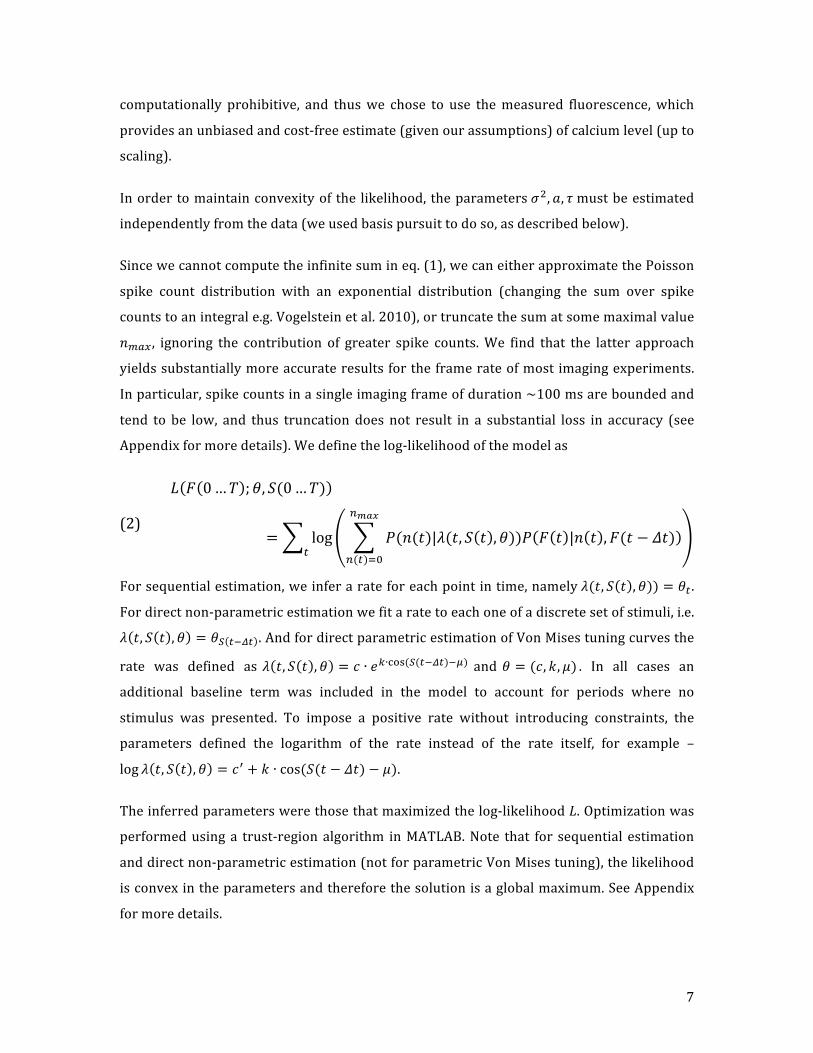
computationally prohibitive, and thuswe chose to use themeasured fluorescence,which

providesanunbiasedandcost-freeestimate(givenourassumptions)ofcalciumlevel(upto

scaling).

Inordertomaintainconvexityofthe likelihood,theparameters𝜎!, 𝑎, 𝜏mustbeestimated

independentlyfromthedata(weusedbasispursuittodoso,asdescribedbelow).

Sincewecannotcomputetheinfinitesumineq.(1),wecaneitherapproximatethePoisson

spike count distribution with an exponential distribution (changing the sum over spike

countstoanintegrale.g.Vogelsteinetal.2010),ortruncatethesumatsomemaximalvalue

𝑛!"# , ignoring the contribution of greater spike counts.We find that the latter approach

yieldssubstantiallymoreaccurateresultsfortheframerateofmostimagingexperiments.

Inparticular,spikecountsinasingleimagingframeofduration~100msareboundedand

tend to be low, and thus truncation does not result in a substantial loss in accuracy (see

Appendixformoredetails).Wedefinethelog-likelihoodofthemodelas

(2)

𝐿 𝐹 0…𝑇 ;𝜃, 𝑆(0…𝑇)

= log 𝑃(𝑛(𝑡)|𝜆(𝑡, 𝑆 𝑡 ,𝜃))𝑃 𝐹 𝑡 |𝑛 𝑡 ,𝐹(𝑡 − 𝛥𝑡)!!"#

!(!)!!!

Forsequentialestimation,weinferarateforeachpointintime,namely𝜆(𝑡, 𝑆 𝑡 , 𝜃)) = 𝜃! .

Fordirectnon-parametricestimationwefitaratetoeachoneofadiscretesetofstimuli,i.e.

𝜆 𝑡, 𝑆 𝑡 , 𝜃 = 𝜃! !!!" .AndfordirectparametricestimationofVonMisestuningcurvesthe

rate was defined as𝜆 𝑡, 𝑆 𝑡 , 𝜃 = 𝑐 ∙ 𝑒!∙!"#(!(!!!")!!) and𝜃 = (𝑐, 𝑘, 𝜇) . In all cases an

additional baseline term was included in the model to account for periods where no

stimulus was presented. To impose a positive rate without introducing constraints, the

parameters defined the logarithm of the rate instead of the rate itself, for example –

log 𝜆 𝑡, 𝑆 𝑡 , 𝜃 = 𝑐! + 𝑘 ∙ cos(𝑆(𝑡 − 𝛥𝑡) − 𝜇).

Theinferredparameterswerethosethatmaximizedthelog-likelihoodL.Optimizationwas

performedusinga trust-regionalgorithm inMATLAB.Note that for sequential estimation

anddirectnon-parametricestimation(notforparametricVonMisestuning),thelikelihood

isconvexintheparametersandthereforethesolutionisaglobalmaximum.SeeAppendix

formoredetails.

8

To implement a smoothness prior we added a term penalizing the sum of squared

differences between neighboring pixels in the rate map (8 neighbors per pixel; toroidal

boundary conditions) to eq. (2). We implemented this prior in the relevant section of

Results.Forallothersectionsnosmoothingorpostprocessingwasperformed.

Figure 1. Graphical representation ofmodel assumptions and dependencies. The only observable

variablesare the stimuluss(t) and the fluorescence f(t) , the restarehidden.Alldependenciesare

instantaneous and simultaneous in time, except calcium levels which depend on values at the

previoustimestep(throughexponentialdecay),and(potentially)thestimulushistory.

Surrogatedata

Surrogatedataweregeneratedfollowingtheschemeinfig.1:(1)Aratewaschosen,either

bysamplingfromaGaussiandistribution,orasadeterministic(tuningcurve)functionofa

time-varying stimulus,𝜆 𝑡 = 𝑓(𝜃, 𝑆 𝑡 ), where𝜃are the parameters defining the tuning,

and𝑆(𝑡)representsthestimulus.𝑆 𝑡 maybemultidimensionalandcanincludehistoryup

to (butnot including) time t.Whenneural couplingwas inferred,we simply replaced the

stimulus with the fluorescence of the coupled neuron, i.e. 𝜆 𝑡 = 𝑓(𝜃,𝐹! 𝑡 ) . 𝐹! 𝑡

representsthefluorescenceofthecoupledneuron,andmayincludehistoryupto(butnot

including)timet.(2)SpikecountsweregeneratedbysamplingfromaPoissondistribution

with the given rate𝑛 𝑡 ~𝑃𝑜𝑖(𝜆 𝑡 ). (3) A calcium levelwas generated by convolving the

spike countwith an exponentially decaying filter, (i.e. spikes in each time bin caused an

instantaneous increase in calcium proportional to the spike count, followed by an

exponential decay). (4) Finally, the fluorescence tracewas generated by adding Gaussian

stimulus (or other!external covariates)

firing rate

spike count

calcium concentration

measured fluorescence

9

measurementnoise.Unlessnotedotherwise,50 randomlygenerated repeated trialswere

usedineachexperiment.

LinearModel

For comparison we also fit the data with a linear model,𝐹 = 𝑘 ∗ (𝐴 ∙ 𝑆), where F is the

fluorescencetrace,Aisacoefficientmatrix(containingtuningparameters),Sisthestimulus

matrix,andkistheexponentialdecayfilterthatcapturesthecalciumdynamics.Thismodel

predicts a fluorescence level for each stimulus value. The equation is linear in the tuning

curve (contained in A), which can thus be estimated using conventional (least-squares)

regression.

ExperimentalProcedures

AllexperimentalprocedureswereconductedinaccordancewiththeUKAnimalsScientific

ProceduresAct (1986). ExperimentswereperformedatUniversityCollegeLondonunder

personal and project licenses released by the Home Office following appropriate ethics

review.

Surgicalproceduresandexpressionofcalciumindicator

ExperimentswereperformedeitherinCamk2a-tTA;EMX1-Cre;Ai93(TITL-GCamp6f)triple

transgenic mice (Madisen et al. 2015), expressing calcium indicator GCaMP6f in all the

corticalCamk2a-positiveexcitatoryneurons,orinwildtypeC57BL6/jmicewhereGCaMP6f

wasexpressedinallneuronsofalocalregionusingavirusinjection.

Usingaseptictechniques,micewereimplantedwithacranialwindowovertherightvisual

cortexaspreviouslydescribed(Andermann,Kerlin,andReid2010;Andermannetal.2011).

An analgesic (Rimadyl, 5mg/Kg, SC)was administered on the day of the surgery and in

subsequent days, as needed. Dexamethasone (0.5 mg/kg, IM) was administered 30 min

priortothesurgerytopreventbrainedema.TheanimalwasanesthetizedwithIsoflurane

(1-2% in 100%Oxygen), body temperaturewasmonitored and kept at 37-38 °C using a

closed-loop heating pad, and the eyes were protected with ophthalmic gel (Viscotears

LiquidGel,AlconInc.).Theheadwasshavedanddisinfected,thecraniumwasexposedand

coveredwithbiocompatiblecyanoacrylateglue(Vetbond).Astainlesssteelheadplatewith

a7mmroundopeningwassecuredovertheskullusingdentalcement(Super-BondC&B,

10

SunMedicalCo.Ltd.,Japan).Then,a3-4mmcraniotomywasopenedoverthevisualcortex

(centeredat -3.3mmAP,2.8ML frombregma). Finally, the craniotomywas sealedwith a

glasscranialwindow,attachedtotheskullusingcyanoacrylateglueanddentalcement.The

windowwasassembledfroma5mmouterroundcoverglasscuredto1-2smallerinserts(3

mm,WarnerInstruments,#1thickness)with index-matchedUVcuringadhesive(Norland

#61). The animalwas allowed to recover for at least 4 days before further experimental

procedures.

For the wild type animals, before sealing the craniotomy we injected an

AAV1.Syn.GCaMP6f.WPRE.SV40 virus (100 nl, titer of 2.4e12 GC/ml, UPenn Vector Core)

250-300µmbelowtheV1surface.Virusreachedexpression levelsuitable for imaging~2

weeksaftertheinjection.

Two-photoncalciumimaging

Fortheimagingexperimentsmicewerehead-fixedunderaresonant-scanningtwo-photon

microscope(B-Scope,Thorlabs).Micewere free torunonanairflow-suspendedspherical

treadmillduringtheimagingsessions.ThemicroscopewascontrolledusingScanImagev4.2

(Pologruto, Sabatini, and Svoboda 2003). A lowmagnification (x16) high NA (0.8) water

immersion objective lens (Nikon) was mounted on a piezoelectric z-drive (PIFOC P-

725.4CA,PhysikInstrumente)allowingmulti-planeimaging.Excitationlight(970nm,30-60

mWat the sample)wasprovidedby a femtosecond laser (ChameleonUltra II, Coherent).

Images (512x512 pixels,with field of view of 340-500microns)were acquired at 30Hz.

This high imaging rate was temporally divided into 3-5 different depths spaced 50-60

micronsapart,resultinginanacquisitionrateof6-10Hzperimagingplane.

Visualstimulation

Visual stimuli were generated in Matlab (MathWorks) using the Psychophysics Toolbox

(Brainard 1997; Kleiner et al. 2007) and displayed on 3 gamma-corrected LCDmonitors

(refreshrate60Hz)arrangedat90degreestoeachother.Themousewaspositionedatthe

centerofthisU-shapedarrangementatthedistanceof20cmfromallthreemonitorssothat

themonitors spanned ±135 degrees of horizontal and ±35 degrees of the vertical visual

field of the mouse. For rate mapping experiments we used sparse spatial white noise

stimuli.Patternsofsparseblackandwhitesquares(4.5-7.5degreesofvisualfield)ongray

11

backgroundwerepresentedat5Hz.Theprobabilityofeachsquaretobenotgraywas2-5%

and independentofothersquares.Fororientationtuningexperimentswepresented0.5s

longdriftinggratings(size60degrees,contrast50%,spatialfrequency0.05cpd,temporal

frequency2Hz,4differentphases).Thepositionof thegratingwasselected tomatch the

retinotopiclocationoftheimagedregion.

Datapreprocessing

Weremovedthebaselinefromfluorescencetracesusingrobustlocalregressionestimation

(Ruckstuhletal.2001).Thisprocedurealsoprovidesanestimateofthemeasurementnoise

standard deviation𝜎. The spikes were estimated using basis pursuit denoising (van den

BergandFriedlander2008)andthemagnitude,a,wasset tobe the95thpercentileof the

coefficient values in the solution of the sparse inverse problem. Calcium decay times,𝜏,

were generally set to 0.5 s. All aforementioned values were inspected manually and

adjustedifnecessary.

12

ResultsGiven fluorescencemeasurements, and stimuli, behavior, or other external covariates,we

estimateratesdirectlybymaximizingthelikelihoodgiveninEq.(2)(seeMethods).Unlike

deconvolution approaches, which aim to explicitly infer spikes, our approach integrates

overtheunobservedspikes,directlyinferringtheunderlyingrate.

Todeconvolveornottodeconvolve?

Asan illustrativeexample,considertheubiquitoustaskofestimatingthemeanfiringrate

acrossrepeatedtrials.Theintuitiveapproachwouldbetofirstestimatethespikecount,in

eachtrial,andthenaveragethesecountsacrossrepeatedtrialstoobtainrates.Wereferto

thisapproach“sequentialestimation”.Alternatively,ourmethodaimstoestimatetherate

directlyfromthecalciummeasurementsacrossallrepeatedtrials.Werefertothisas“direct

estimation”.

Figure 2.ASimulatedexampleof temporalsignals in the fluorescencegenerationprocess.Ateach

point in time atmost one of 9 discrete stimuli is ‘on’ (1st row). Each stimulus is deterministically

associatedwitharate(2ndrow).SpikecountsaresamplesfromaPoissonprocesswiththegivenrate

(3rdrow).Calciumlevelsareaconvolutionof thespikecountswithanexponential filter– i.e.each

spikecausesaninstantaneousriseincalciumfollowedbyanexponentialdecay(4throw).Finally,the

measured fluorescence is a scaled version of the calcium, corrupted with Gaussian measurement

13

noise (5th row). The goal is to estimate the relationship between stimulus and rate, given the

observedfluorescencesignal.

To compare the two approaches, we generated data as illustrated in Fig. 2. Fifty noisy

repeatswith the same underlying ratewere randomly generated. The log of the rate for

eachtimebinwasdrawnfromaNormaldistribution(𝜇 = −4,𝜎 = 1.5).Wethenestimated

therate inoneof threeways:(a)By fittingeq. (2) fromMethodssimultaneously toall50

repeats;(b)Byfittingeq.(2)toeachindividualrepeatandaveragingacrossrepeats;and(c)

Byusingthedeconvolutionmethodof(Vogelsteinetal.2010)toestimatespikecount/rate

on each repeat, and averaging these across repeats. As can be seen in fig. 3A, fitting all

repeatssimultaneouslysubstantiallyimprovestheestimateoftherate.Moreover,estimates

basedonaveragingsingle trialsdonotconverge to the truevalueof therate.Thisoccurs

because lowratesare systematicallyoverestimated– forvery low(orzero) spikecounts,

the effects ofmeasurement noise are asymmetric, generally leading to an increase in the

numberofestimatedspikes,sincethenumberofspikesmustremainnon-negative.

Wealsonotethatevenifthegoaloftheanalysisistoestimatethespikecountineachtime

bin, our approach provides a more accurate estimate of the spike count than the

deconvolutionapproach(fig.3B).Thisisaconsequenceofthefactthatweexplicitlymodel

atimevaryingrate,andassumethatspikecountsfollowaPoissondistribution(whichisthe

truedistributionforthesimulateddata).Therefore,fortheremainderofthisarticle,wewill

usetherateestimatesfromeq.(2)averagedacrosstrialstoperformsequentialestimation,

ratherthanaveragingspikecountestimatesprovidedbydeconvolution.

Figure 3. Estimating rates and spike counts from simulated calcium fluorescence data. A. 50

fluorescence traceswith the same underlying ratewere randomly generated (measurement noise

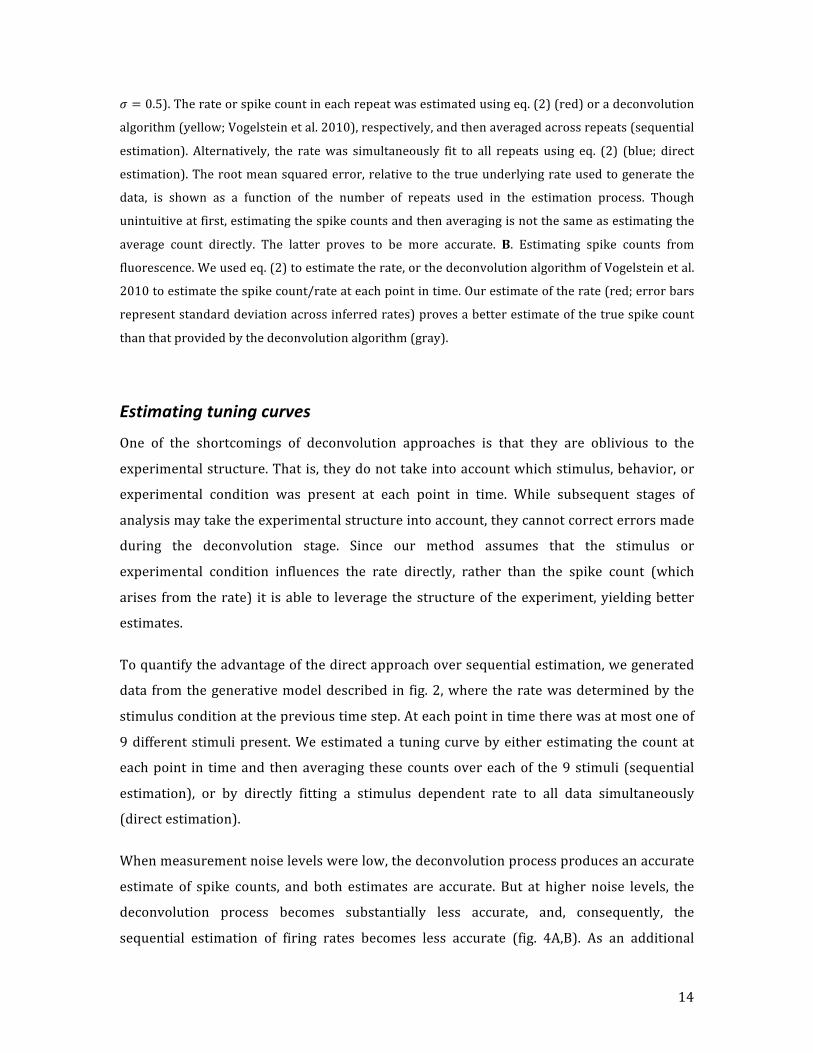
14

𝜎 = 0.5).Therateorspikecountineachrepeatwasestimatedusingeq.(2)(red)oradeconvolution

algorithm(yellow;Vogelsteinetal.2010),respectively,andthenaveragedacrossrepeats(sequential

estimation). Alternatively, the ratewas simultaneously fit to all repeats using eq. (2) (blue; direct

estimation).Therootmeansquarederror,relativetothetrueunderlyingrateusedtogeneratethe

data, is shown as a function of the number of repeats used in the estimation process. Though

unintuitiveatfirst,estimatingthespikecountsandthenaveragingisnotthesameasestimatingthe

average count directly. The latter proves to be more accurate. B. Estimating spike counts from

fluorescence.Weusedeq.(2)toestimatetherate,orthedeconvolutionalgorithmofVogelsteinetal.

2010toestimatethespikecount/rateateachpointintime.Ourestimateoftherate(red;errorbars

representstandarddeviationacrossinferredrates)provesabetterestimateofthetruespikecount

thanthatprovidedbythedeconvolutionalgorithm(gray).

Estimatingtuningcurves

One of the shortcomings of deconvolution approaches is that they are oblivious to the

experimentalstructure.Thatis,theydonottakeintoaccountwhichstimulus,behavior,or

experimental condition was present at each point in time. While subsequent stages of

analysismaytaketheexperimentalstructureintoaccount,theycannotcorrecterrorsmade

during the deconvolution stage. Since our method assumes that the stimulus or

experimental condition influences the rate directly, rather than the spike count (which

arises fromtherate) it isable to leverage thestructureof theexperiment,yieldingbetter

estimates.

Toquantifytheadvantageofthedirectapproachoversequentialestimation,wegenerated

data fromthegenerativemodeldescribed in fig.2,wheretheratewasdeterminedbythe

stimulusconditionattheprevioustimestep.Ateachpointintimetherewasatmostoneof

9differentstimulipresent.Weestimateda tuningcurvebyeitherestimating thecountat

eachpoint in timeand thenaveraging thesecountsovereachof the9stimuli (sequential

estimation), or by directly fitting a stimulus dependent rate to all data simultaneously

(directestimation).

Whenmeasurementnoiselevelswerelow,thedeconvolutionprocessproducesanaccurate

estimate of spike counts, and both estimates are accurate. But at higher noise levels, the

deconvolution process becomes substantially less accurate, and, consequently, the

sequential estimation of firing rates becomes less accurate (fig. 4A,B). As an additional

15

comparison,wealso showestimatesderived from linear regression (seemethods).While

linearestimatesare lesssensitive tonoise theyaresubstantially lessaccurate thaneither

sequentialordirectestimation.

Robustness to noise is of particular importance in imaging experiments, which are often

designed for high throughput simultaneous measurements frommany cells. The field of

viewofa typical imagingexperimentmayeasilycontain thousandsofneurons,andwhile

somemayberelatively‘clean’manyarenoisy.Toharnessthepotentialofcalciumimaging

onewould like to ‘dig’ as deeply into the data as possible. To this end,we note that the

directestimationmethodrequiresfewersamples(shorterexperiment)toachievethesame

accuracy as sequential estimation (fig. 4C). This is of particular importance for imaging

experiments carried out in awake head-fixed animals in which animal welfare

considerationsdictatestrictlimitsonexperimentalduration.

16

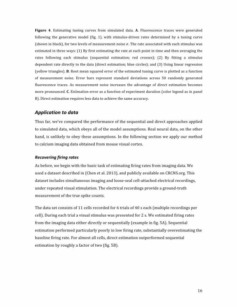
Figure 4. Estimating tuning curves from simulated data. A. Fluorescence traces were generated

following the generative model (fig. 1), with stimulus-driven rates determined by a tuning curve

(showninblack),fortwolevelsofmeasurementnoise𝜎.Therateassociatedwitheachstimuluswas

estimatedinthreeways:(1)Byfirstestimatingtherateateachpointintimeandthenaveragingthe

rates following each stimulus (sequential estimation; red crosses); (2) By fitting a stimulus

dependentratedirectlytothedata(directestimation;bluecircles);and(3)Usinglinearregression

(yellowtriangles).B.Rootmeansquarederroroftheestimatedtuningcurveisplottedasafunction

of measurement noise. Error bars represent standard deviations across 50 randomly generated

fluorescence traces. As measurement noise increases the advantage of direct estimation becomes

morepronounced.C.Estimationerrorasafunctionofexperimentduration(colorlegendasinpanel

B).Directestimationrequireslessdatatoachievethesameaccuracy.

Applicationtodata

Thusfar,we’vecomparedtheperformanceofthesequentialanddirectapproachesapplied

tosimulateddata,whichobeysallofthemodelassumptions.Realneuraldata,ontheother

hand,isunlikelytoobeytheseassumptions.Inthefollowingsectionweapplyourmethod

tocalciumimagingdataobtainedfrommousevisualcortex.

Recoveringfiringrates

Asbefore,webeginwiththebasictaskofestimatingfiringratesfromimagingdata.We

usedadatasetdescribedin(Chenetal.2013),andpubliclyavailableonCRCNS.org.This

datasetincludessimultaneousimagingandloose-sealcell-attachedelectricalrecordings,

underrepeatedvisualstimulation.Theelectricalrecordingsprovideaground-truth

measurementofthetruespikecounts.

Thedatasetconsistsof11cellsrecordedfor6trialsof40seach(multiplerecordingsper

cell).Duringeachtrialavisualstimuluswaspresentedfor2s.Weestimatedfiringrates

fromtheimagingdataeitherdirectlyorsequentially(exampleinfig.5A).Sequential

estimationperformedparticularlypoorlyinlowfiringrate,substantiallyoverestimatingthe

baselinefiringrate.Foralmostallcells,directestimationoutperformedsequential

estimationbyroughlyafactoroftwo(fig.5B).

17

Figure5.Estimatingfiringratesfromsimultaneousimagingandelectricalrecordings.A.Themean

firingrateacrossrepeatsforanexamplecellwasestimatedeitherbyaveragingelectricallyrecorded

spikecountsacross40repeatedtrials(black),byaveragingspikecountsinferredfromindividual

trialsofimagingdata(bottom;red;sequential),orbydirectlyestimatingtherateacrosstrialsfrom

imagingdata(top;blue;direct).B.Rootmeansquarederror(relativetotherateestimatedfrom

electricalrecordings)ofthesequentialmethodisplottedagainstthatofthedirectmethod(blackline

indicatesequality).Eachpointcorrespondstoestimatesforasinglecell,obtainedon40repeatsofa

6sstimulus(n=24recordings).RedpointcorrespondstotheexampleinpanelA.

Estimatingratemaps

Next,weappliedourapproachtoestimatetheratemapsofneuronsinmousevisualcortex.

Micewerehead-fixedona floatingballandviewedsparsenoisestimulionascreenwhile

calciumactivity(reportedbyGCaMP6f)wasrecordedusingatwo-photonmicroscope(see

Methods fordetails).Thestimuluswasa10x36squarepixelgrid,whereeachpixelhada

2.5%chanceofbeingeitherwhiteorblackanda95%chanceofbeinggray.Thegoalofthe

analysiswastoidentifytheregioninthevisualfieldinwhichchangestothelightaffectthe

neuron’sresponse.

As in the previous sections, we estimated the rate associatedwith a pixel either by first

estimating therate ineach timebin,and thenaveragingall timebins forwhich thatpixel

wasblack/white (sequential estimation),orbydirectly fittingapixel-intensitydependent

ratetothedata(directestimation).

Figure6Ashowsthe inferredratemaps foranexampleneuron.Thiscorresponds toeach

model’sexpectedrategiveneachpixelbeingblack, independentofotherpixels. Since the

stimulus is sparse (see methods) interactions between pixels are negligible. Visual

18

inspectionrevealsthatthesequentialapproachproducesanoisierestimateoftheratemap.

Wequantifiedthenoise level intheratemapusingthemedianabsolutedeviation(MAD).

We chose the MAD over the standard deviation as a measure of variability/noisiness,

becauseitislesssensitivetooutliersarisingattheextremaoftheratemaps.Forallcellsin

this data set exhibiting clear ratemap structure, fitting the data directlywith a position-

dependentrateresultedinlessnoisyratemapestimatescomparedtoasequentialestimate

orlinearregression(fig.6B).

19

Figure 6. Estimating rate maps from data. A. Rate maps of mouse visual cortical neurons were

estimated using direct estimation (top), sequential estimation (middle) and linear regression

(bottom; see text for details). The intensity of eachpixel represents the rate (rescaled) associated

with that pixel being black (this is an off cell). The direct estimation approach provides the least

noisyestimateof the ratemap(nosmoothingor regularizationwasapplied).B.Thequalityof the

ratemapestimatewasquantifiedusingthemedianabsolutedeviation(MAD)oftheentireratemap.

TheMAD for the sequential estimates (red) and linear regression (yellow) are plotted against the

MADforthedirectestimates(n=9neurons;circleddatapointscorrespondtotheexampleinpanel

A).Forallcellsthedirectestimateprovedleastnoisy.

Abovewemeasured the ‘goodness’ of the ratemapsbymeasuring their smoothness.Our

framework is sufficiently general thatwe can explicitly incorporate this prior knowledge

about the smoothnessof ratemaps into themodel.This canbedonebyaddingapenalty

proportional to the sum of squared differences between neighboring pixels to the log

likelihood. In fig. 7 we show the impact of adding a smoothness prior on rate map

estimation.Note thathere forclarityweshowthe linearportionofourmodel,before the

nonlinearity,andthusalog-ratemap.

Figure 7. Estimating ratemapswith a prior preference for smoothness.A. The linear spatial filter

portionofthemodelestimatedforanexampleneuronfromresponsestoasparsenoisestimulus.B.

ThesameaspanelA,butwiththesmoothnesspriorimposed.

Estimatingparametricorientationtuning

We now turn to the problem of estimating orientation tuning curves from responses to

drifting grating stimuli (same neurons as in previous section; see Methods). Orientation

tuning curves are often summarized by a scaled Von Mises probability density function

20

(Swindale1998),which isdefinedbyonlythreeparameters–mean,widthandscale.The

meanoftheVonMisesfitisthepreferredorientationoftheneuron.

Thiswidelyusedparametricformofthetuningcurveallowsustohighlightanotherfeature

of our model. Since we explicitly model the relationship between the stimulus and the

response,theparametricformmaybeincorporatedintotheobjectivefunction,allowingus

todirectlyestimatetheparameters(notethattheparametricformcanimpacttheconvexity

of the likelihood, and thus the complexity of the optimization problem; see appendix for

more details). For comparison, we also consider a sequential scheme, in which we first

estimateratesonindividualtrials,thenaveragethem,andfinallyfitaVonMisesfunctionto

theseaverages.

Toassessthequalityofthefittedtuningcurves,wemeasuredthevariabilityoftheestimate

across randomly selected subsets of the data. A better estimator should exhibit less

variabilityacrossthedifferentsubsets.

With limited data (less than 5minutes) estimating the parameters defining a VonMises

tuning curve directly from the data provesmore reliable (fig. 8) compared to sequential

estimation.Thisisbecauseweareonlyfitting3parameterstotheentiretrace,andweare

taking intoconsiderationanyuncertainty thatwehave in theestimatesof therate. In the

sequentialapproach,eachstage isoblivious toanyuncertainties in thepreviousstage.As

the amount of data increases, both approaches perform consistently, but this is partially

becausetheoverlapbetweentherandomlychosensubsetsnecessarilyincreases.

Figure 8. Estimatingorientation tuning curves fromdata.A.Orientation tuningcurvesof amouse

visual cortical neuronwas estimated either sequentially (estimating rates and then averaging the

ratesassociatedwitheachorientation;redcircles),orbydirectlyfittingaparametricallydefinedVon

21

Mises shaped tuning curve directly to the fluorescence data (blue curve). B. Subsets of data of

differentlengthswererandomlyselectedandthetuningoftheneuronwasestimated.Thestandard

deviation of these estimates is plotted as a function of the length of the subset used for the

estimation.Thedirectparametricapproachprovidesamorereliableestimateofthetuningforany

givenamountofdata.

Inferringneuralcoupling

Previous work has demonstrated the value and importance of modeling the coupling

betweenneurons(Pillowetal.2008;Gerhardetal.2013;Okatan,Wilson,andBrown2005).

Neuralcouplingispredominantlymediatedthroughspikesandtheensuingsynapticevents.

Ourdirectinferenceapproach,however,doesnotprovideanestimateofthespikes.Isitstill

possibletoinferneuralcoupling?

Though actual spike times are never inferred throughout our analysis, the observed

fluorescencetraceprovidesanoisyfilteredversionofthespikes.Thereforeweinvestigated

whether coupling between neurons, at the level of spikes, can be inferred using the

fluorescence signal. Note that this analysis can only infer interactions occurring at the

relatively slow sampling rate of the experiment (~10Hz), andnot thoseoccurring at the

timescaleofsynaptictransmission(>100Hz).

To test whether neural coupling can be inferred from fluorescence, we simulated two

neurons, in which the spikes of neuron 2multiplicatively influence the rate of neuron 1

through a predefined temporal filter, cs. We then inferred the rate of neuron 1 from its

fluorescencetrace,usingthefluorescencetraceofneuron2asacovariate(asifitwerean

external stimulus). This procedure provides us with a maximum likelihood estimate of

neuron1’srateandanestimateof thecouplingbetweentheneurons.Wewilldenotethis

inferredfiltercf.Onemustkeepinmindthatcsandcf,arenotexpectedtobeidentical,asthe

formeroperatesonspikeswhilethelatteroperatesdirectlyonthefluorescencesignal.Yet,

itiseasytoseethatifwewanttogenerateafilterwhichwillmimiccf’soutputwhenapplied

to spikes,we simply need to convolve cfwith an exponential filter, the same convolution

processthatconvertsspiketrainstocalciumtraces.Wedenotethisfilter𝑐!.

Asexpected,whiletheinferredfiltercfdoesnotmatchthecouplingfilterusedtogenerate

thedata,onceweconvolveitwithanexponentialdecaytoobtain𝑐!producesaverygood

22

estimateofthetruecouplingbetweentheneurons(fig.9).Thissuggeststhatourapproach

enables inference of spike based coupling between neurons, although spikes are never

inferredintheprocess.

Figure9.Inferringspikebasedcouplingfromfluorescence.A.Therateofneuron1(top)isdirectly

influencedbythespikingactivityofneuron2throughacouplingfiltercs,yetourtaskistoinferthis

coupling by observing fluorescence alone. B. We generated surrogate fluorescence data using a

knowncouplingfiltercs(blackline).Wethenestimatedtheneuralcoupling𝑐!byinferringtherateof

neuron 1 using the fluorescence of neuron 2 as a covariate (a fluorescence dependent rate). The

inferredcouplingcfwasconvolvedwithanexponentialdecaytoobtain𝑐!(bluecircles;seetext for

details).

23

DiscussionWehaveshownthatsequentialestimationofneuralfiringratesfromcalciumimagingdata,

by first estimating spike counts and then averaging these to obtain firing rates and/or

tuning curves, can produce strongly biased results. As an alternative, we’ve developed a

directmethodthatoperatesbyintegratingovertheunobservedspikecounts.Ouranalysis

showsthatdirectestimationoutperformssequentialestimationinsimulation,aswellason

imagingdata.Themethodisflexible,allowingestimationoffiringratedependenciesonany

measuredcovariate(e.g.,movementdirection,locationinspace,taskcondition,behavioral

state), using calcium imaging obtained from either repeated trials, and/or by assuming a

parametricrelationshipbetweencovariatesandfiringrates.

Calciumtracedeconvolution

Theterm“deconvolution”stems fromtheassumptionthat intracellularcalciumlevelscan

bedescribedasaconvolutionofthespiketrainwithalinearfilter.Deconvolutionprovides

anaturalpreprocessing stage for theanalysisof imagingdata, extractingestimatesof the

underlyingspikes,afterwhichstandardmethodsmaybeusedtoanalyzethespikecounts.

Deconvolution algorithms are based on a variety of different methodologies including

Bayesian inference (Vogelstein et al. 2010; Theis et al. 2015), basis pursuit (Grewe et al.

2010),matchingpursuit (Dyeret al. 2010), amongothers (Oñativia, Schultz, andDragotti

2013).Themethodof(Vogelsteinetal.2010),inparticular,isbasedonthesamegenerative

modelwehaveused in this article. Butourdirectmethoddiffers in that: (a) it explicitly

includesa stimulus-dependent, timevarying rate,whereas in (Vogelsteinet al., 2010) the

rate is fixed and is used as a sparse prior on spike counts; (b) it integrates over the

unobservedspikecounts,ratherthanattemptingtoexplicitlyestimatethem;(c)itassumes

a Poisson spiking process, rather than substituting a more computationally tractable

exponentialdistribution.

These differences, while seemingly minor, result in substantial improvements in the

accuracyofratesinferredfromcalciumdata(seefig.3).Inparticular,thepresenceofnoise

in the imaging process ensures that the deconvolution results will be imperfect, but

subsequent analyses generally ignore the uncertainty associated with the spike count

estimates.Aswehaveshownthiscanleadtobiaseswhenestimatingfiringratesandtuning

curvesfromthedata,especiallyforlowfiringrates.Byintegratingoutthespikecountswe

24

are able to take theuncertainty associatedwith spike count estimation into account, and

consequently provide a procedure that ismore tolerant to noise. Furthermore, the direct

approach proves more statistically efficient, which in practice can translate into shorter

experiments.

Similarargumentsinfavorofdirectestimationhavebeenmadeinthepastwithregardto

spikesorting.Namelyithasbeenshownthatitmaybepreferableestimatetuningcurves

directlyfromrawvoltagetraces,ratherthantofirstsortthespikesandthenfitthetuning

curves(Ventura2009b;Ventura2009a).Recentlyitwasshownthatananimal’spositionin

spacecanbedecodedwithbetteraccuracydirectlyfromhippocampalspikewaveforms,

thanbyasequentialschemeinwhichspikesarefirstsortedandthenusedforposition

estimation(Kloostermanetal.2014;Dengetal.2015).

Forbothspikesortinganddeconvolutionitisimportanttorememberthattheoutputofany

algorithmisonlyanestimateofspiketimes/counts,andshouldbetreatedassuch.

Subsequentanalysesthatignoretheuncertaintyintheseestimatesmayaccumulateerrors

andbiases.Thisisnotaproblemwhenthesignaltonoiseratioisverylargeandspikescan

berecoveredwithhighaccuracy,yetthesecasesareincreasinglyrareashigh-throughput

physiologicalrecordingsarebecomingmoreprevalent.

Modelassumptions

Theelementsofourmodelarecommonplaceintheliterature,andarenotuniquetoour

approach,suchasPoissonspiking(DayanandAbbott2001)orGaussianmeasurement

noise(Wilt,Fitzgerald,andSchnitzer2013).

Anadditionalassumption,centraltomostdeconvolutionapproaches,isthatcalciumlevels

aretheresultofalinearconvolutionofthespiketrainwithanexponentialdecayfilter.In

general,peakcalciumlevelsarenotdirectlyproportionaltospikecount,anddecaytimecan

varywithspikecount(Akerboometal.2012;Baduraetal.2014;Chenetal.2013).These

observationsmaybeexplainedbynon-linearsummationofspike‘signatures’(Nauhaus,

Nielsen,andCallaway2012),whichismostpronouncedforhighfiringrates.Itisnot

immediatelyclearhowtoincorporateanonlinearityintotheconvolutionprocessinour

generativemodelwhilemaintainingcomputationaltractability,thusitmaybeadvisableto

remainnearthelinearoperatingregimeoftheindicator.Furtherweassumethatthespike

25

‘signature’includesaninstantaneousrise.Althoughthisisanidealization,forimaging

experimentswiththelatestcalciumindicatorstherisetimeistypicallyontheorderofthe

samplingrate.Thuswedonotexpectthisassumptiontogreatlyaffectthemodel.

Regionofinterest

AseeminglyindependentproblemwhenanalyzingimagingdataisthatofRegionOfInterest

(ROI)detection(Mukamel,Nimmerjahn,andSchnitzer2009).Recentlyseveralgroupshave

notedthattheROIdetectionanddeconvolutionproblemsareinfactrelated.Knowledgeof

spiketimescanclearlyguideROIdetectionandviceversa.Consequentlysomeauthorshave

exploredthecombinationofthesetwoanalysisstepsintoasingleoptimizationproblem,

tryingtosolvefortheROIsandspiketimes/countssimultaneously(DiegoAndillaand

Hamprecht2014;Pnevmatikakisetal.2014).Followingourinsightsfromthecurrentwork,

wesuggestthatwhenthegoaloftheanalysisisrate(ortuningcurve)estimation,itmay

provebeneficialtoestimatetheratedirectlyfromtherawimages.Thismayprovetobea

computationallyprohibitivetaskandwedeferthisforfutureresearch.

Conclusion

Asimagingmethodsbecomeanincreasinglypopularwaytomeasurebrainactivity,itis

importanttodevelopalgorithmstoanalyzethesedata.Wechosetofocusonexperimentsin

whichthegoaloftheanalysisisafiringrate,anaveragespikecounthistogram,oratuning

curve.Althoughthisdoesnotencompassallpossibleanalyses,itissufficientlybroadto

includeawiderangeofexperiments.

Wearguethatthe‘correct’approachtothisestimationproblemistointegrateoutthe

unobservedspikestoobtainthequantitiesofinterest.Analogousproposalshavebeenmade

inthecontextofelectrophysiologicaldata(Ventura2009b;Ventura2009a;Kloostermanet

al.2014;Dengetal.2015).Properlyintegratingover“nuisancevariables”isawell-known

themeinthestatisticalestimationandmachinelearningcommunities,butisnotoriousfor

beingcomputationallyexpensive.Ourdirectmethodofestimatingfiringratesandtuning

26

curvesfromimagingdataprovidesstate-of-the-artestimatesofratesbyintegratingoutthe

spikecounts,yetisefficientenoughtorunonastandardcomputer.

AcknowledgementsThisworkwassupportedbytheJamesS.McDonnellFoundation(EG),theWellcomeTrust

(LFR,MK,andMC),andtheHowardHughesMedicalInstitute(EPS).MCholdsthe

GlaxoSmithKline/FightforSightChairinVisualNeuroscience.

27

Appendix

Propertiesofthemodellikelihood

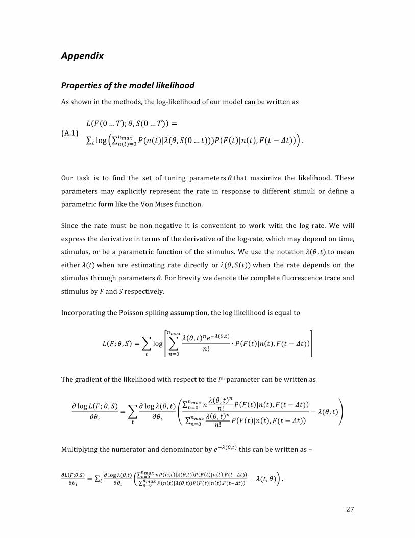
Asshowninthemethods,thelog-likelihoodofourmodelcanbewrittenas

(A.1)𝐿 𝐹 0…𝑇 ;𝜃, 𝑆(0…𝑇) =

log 𝑃(𝑛(𝑡)|𝜆(𝜃, 𝑆(0… 𝑡)))𝑃 𝐹 𝑡 |𝑛 𝑡 ,𝐹(𝑡 − 𝛥𝑡)!!"#!(!)!!! .

Our task is to find the set of tuning parameters𝜃that maximize the likelihood. These

parametersmay explicitly represent the rate in response to different stimuli or define a

parametricformliketheVonMisesfunction.

Since the rate must be non-negative it is convenient to work with the log-rate. We will

expressthederivativeintermsofthederivativeofthelog-rate,whichmaydependontime,

stimulus,orbeaparametric functionof thestimulus.Weuse thenotation𝜆(𝜃, 𝑡)tomean

either𝜆(𝑡)when are estimating rate directly or𝜆(𝜃, 𝑆 𝑡 )when the rate depends on the

stimulusthroughparameters𝜃.Forbrevitywedenotethecompletefluorescencetraceand

stimulusbyFandSrespectively.

IncorporatingthePoissonspikingassumption,theloglikelihoodisequalto

𝐿 𝐹; 𝜃, 𝑆 = log𝜆 𝜃, 𝑡 !𝑒!!(!,!)

𝑛!∙ 𝑃 𝐹 𝑡 |𝑛 𝑡 ,𝐹(𝑡 − 𝛥𝑡)

!!"#

!!!!

Thegradientofthelikelihoodwithrespecttotheithparametercanbewrittenas

𝜕 log 𝐿 𝐹; 𝜃, 𝑆𝜕𝜃!

=𝜕 log 𝜆(𝜃, 𝑡)

𝜕𝜃!

𝑛 𝜆 𝜃, 𝑡!

𝑛! 𝑃 𝐹 𝑡 |𝑛 𝑡 ,𝐹(𝑡 − 𝛥𝑡)!!"#!!!

𝜆 𝜃, 𝑡 !

𝑛! 𝑃 𝐹 𝑡 |𝑛 𝑡 ,𝐹(𝑡 − 𝛥𝑡)!!"#!!!

− 𝜆(𝜃, 𝑡)!

Multiplyingthenumeratoranddenominatorby𝑒!!(!,!)thiscanbewrittenas–

!" !;!,!!!!

= ! !"#!(!,!)!!!

!" ! ! !(!,!) ! ! ! |! ! ,!(!!!")!!"#!!!

! ! ! !(!,!) ! ! ! |! ! ,!(!!!")!!"#!!!

− 𝜆(𝑡, 𝜃)! .

28

TheentriesoftheHessianaretherefore

!!! !;!,!!!!!!

= − ! !"#!(!,!)!!!

! !"#!(!,!)!!!

𝜆(𝜃, 𝑡) − !!! ! ! !(!,!) ! ! ! |! ! ,!(!!!")!!"#!!!

! ! ! !(!,!) ! ! ! |! ! ,!(!!!")!!"#!!!

+!

!" ! ! !(!,!) ! ! ! |! ! ,!(!!!")!!"#!!!

! ! ! !(!,!) ! ! ! |! ! ,!(!!!")!!"#!!!

!+

!!!"#$(!,!)!!!!!

!" ! ! !(!,!) ! ! ! |! ! ,!(!!!")!!"#!!!

! ! ! !(!,!) ! ! ! |! ! ,!(!!!")!!"#!!!

− 𝜆(𝜃, 𝑡)! .

Note that if!!!"#$(!,!)!!!!!

= 0(which is the case for sequential estimation or direct non-

parametricestimation)thenthenegativeHessianispositivesemi-definiteandthenegative

log-likelihood is thus convex. To see this, let us denote the term in square brackets k(t),! !"#!(!,!)

!!!= q!(𝑡), and𝑣 𝑡 = 𝑘 𝑡 q(𝑡). Thus we can write !

!!!!!!!

= −! 𝑣(𝑡)𝑣(𝑡)! , i.e. a

sum of outer products of a vector with itself. Therefore the negative Hessian is positive

semi-definite.

Exponentialapproximation

Asnotedinthemaintext,itispossibletosubstitutetheassumptionofPoissonspikingwith

exponentially distributed ‘counts’ (these are not truly counts since they are no longer

integers). In thiscase integratingout thespikescanbedonemoreefficiently.Namely, the

sum

𝑃 𝐹 𝑡 , 𝑛 𝑡 𝜆(𝑡),𝐹(0… 𝑡)∞

! ! !!

ineq.(1)inMethodsisreplacedbyanintegral–

𝑃 𝐹 𝑡 , 𝑛 𝑡 𝜆(𝑡),𝐹(0… 𝑡) 𝑑𝑛(𝑡)∞

!

Inaddition,now𝑃 𝑛 𝑡 𝜆 𝑡 = 𝜆 𝑡 𝑒!! ! !(!).

29

Thoughwedidnotachievegoodresultswiththisapproximation,wepresenttheequations

forthelog-likelihood,gradient,andHessianforcompleteness.Forbrevitywewilldropthe

explicitdependenceof𝜆on𝜃.

𝐿 𝐹; 𝜃 = log 𝜆 𝑡 − 𝜆 𝑡 𝐹 𝑡 + log𝐾!(𝑡)!

𝜕𝐿 𝐹; 𝜃𝜕𝜃!

=𝜕 log 𝜆 𝑡𝜕𝜃!

1 − 𝜆 𝑡 𝐹 𝑡 −𝑧 𝑡 𝜎𝜆 𝑡𝐾!(𝑡)

+ 𝜆 𝑡 𝜎 !

!

𝜕!𝐿 𝐹; 𝜃𝜕𝜃!𝜃!

=𝜕 log 𝜆(𝑡)𝜕𝜃!

𝜕 log 𝜆(𝑡)𝜕𝜃!

−𝜆 𝑡 𝐹 𝑡 + 2𝜎𝜆! 𝑡!

−𝜎𝑧 𝑡 𝜆 𝑡𝐾!(𝑡)

𝜆 𝑡 𝐹 𝑡 + 𝜎𝜆 𝑡𝑧 𝑡𝐾! 𝑡

− 𝜎𝜆(𝑡) + 1

+𝜕!𝑙𝑜𝑔𝜆(𝑡)𝜕𝜃!𝜃!

1 − 𝜆 𝑡 𝐹 𝑡 −𝑧 𝑡 𝜎𝜆 𝑡𝐾!(𝑡)

+ 𝜆 𝑡 𝜎 !

!

Wherewedefinethefollowingintermediatequantities–

𝐹 𝑡 =1𝑎

𝐹 𝑡 − 𝛥𝑡 𝑒!!"! − 𝐹 𝑡

𝐾! 𝑡 =𝜋2exp

𝜆 𝑡 𝜎 !

2∙ erfc

𝜆 𝑡 𝜎 − 𝐹𝜎2

𝑧 𝑡 = exp −12

𝐹(𝑡)𝜎

!

+ 𝜆 𝑡 𝐹(𝑡)

Implementationconsiderations

There are 3 keys to making the task of integrating out the spike count computationally

efficient:(1)TheassumptionthatFluorescenceisconditionallyindependentofthespiking

historygiven the fluorescenceat theprevious timestepandthecurrentspikecount.This

30

allowsus toavoidacombinatorialexplosion, sinceweonlyneed tosumoverallpossible

spike counts at the current time step alone. (2) The observation that probability of

observing a certain fluorescence value at time t, given the spike count at time t and the

fluorescence at the previous time step,𝐹 𝑡 |𝑛 𝑡 ,𝐹 𝑡 − 𝛥𝑡 , does not depend on the

parameters being optimized. This means that we can calculate this quantity once for

differentvaluesofn(t)anddonotneedtoreevaluateitduringoptimizationiterations.(3)

The truncation of the sum in eq. (1) ofMethods,which ignores the contribution of large

spikecounts.Sincethespikecount tendstobesmall forourchoiceof timebins, thissum

canbesafelytruncatedatanappropriatenumber,whichwedesignateasnmax.

A proper choice of nmax depends on the preparation and the sampling rate. The data

analyzedinthisstudycomesfromneuronsinthesuperficiallayersofmousevisualcortex.

Electrophysiologysuggeststhatsuchneuronsrarelyspikeatratesthatexceed~20Hz(Niell

andStryker2008).Atasamplingrateof6Hz(asinourdata)thismeanslessthan4spikes

perbin.Weusedanmaxvalueof~10spikes/bin,whichisequivalentto~60spikes/s.Tobe

onthesafesidethough,weincreasedthevalueofnmaxfrom6to25spikes/bin,butdidnot

observeassubstantialeffectontheratemapestimate(fig.A.1A).

Toachievethebestruntimenmaxshouldbesetaslowaspossible,butascanbeseeninfig.

A.1B,fittinga10x36ratemapusingourmethodtakesabout0.1secondsforawiderangeof

nmaxvalues(ona2014AppleMacBookProlaptop).

31

FigureA.1.Settingthemaximalspikerateanditseffectonruntime.A.Thesameratemapasinfig.6

wasfitusingdifferentvaluesofnmax.Changingnmaxfrom36Hzto150Hzhasnovisibleeffectonthe

inferred ratemap.B. The time it takes to fit the10x36 ratemap shown inpanelA is plotted as a

functionofnmax.Fornmaxvaluesofupto150Hztheruntimeisaround0.1seconds.

32

References

Akerboom,Jasper,Tsai-WenChen,TrevorJ.Wardill,LinTian,JonathanS.Marvin,SevinçMutlu,NicoleCarrerasCalderón,etal.2012.“OptimizationofaGCaMPCalciumIndicatorforNeuralActivityImaging.”TheJournalofNeuroscience32(40):13819–40.doi:10.1523/JNEUROSCI.2601-12.2012.

Andermann,MarkL,AaronMKerlin,DemetrisKRoumis,LindseyLGlickfeld,andRClayReid.2011.“FunctionalSpecializationofMouseHigherVisualCorticalAreas.”Neuron72(6).ElsevierInc.:1025–39.doi:10.1016/j.neuron.2011.11.013.

Andermann,MarkL,AMKerlin,andRCReid.2010.“ChronicCellularImagingofMouseVisualCortexduringOperantBehaviorandPassiveViewing.”FrontiersinCellularNeuroscience4(January).Frontiers:3.doi:10.3389/fncel.2010.00003.

Badura,Aleksandra,XiaonanRichardSun,AndreaGiovannucci,LauraA.Lynch,andSamuelS.-H.Wang.2014.“FastCalciumSensorProteinsforMonitoringNeuralActivity.”Neurophotonics1(2):025008–025008.doi:10.1117/1.NPh.1.2.025008.

Brainard,DavidH.1997.“ThePsychophysicsToolbox.”SpatialVision10:433–36.Chen,Tsai-Wen,TrevorJ.Wardill,YiSun,StefanR.Pulver,SabineL.Renninger,Amy

Baohan,EricR.Schreiter,etal.2013.“UltrasensitiveFluorescentProteinsforImagingNeuronalActivity.”Nature499(7458):295–300.doi:10.1038/nature12354.

Dayan,Peter,andL.F.Abbott.2001.TheoreticalNeuroscience:ComputationalandMathematicalModelingofNeuralSystems.1sted.TheMITPress.

Deng,Xinyi,DanielF.Liu,KennethKay,LorenM.Frank,andUriT.Eden.2015.“ClusterlessDecodingofPositionfromMultiunitActivityUsingaMarkedPointProcessFilter.”NeuralComputation27(7):1438–60.doi:10.1162/NECO_a_00744.

DiegoAndilla,Ferran,andFredAHamprecht.2014.“SparseSpace-TimeDeconvolutionforCalciumImageAnalysis.”InAdvancesinNeuralInformationProcessingSystems27,editedbyZ.Ghahramani,M.Welling,C.Cortes,N.D.Lawrence,andK.Q.Weinberger,64–72.CurranAssociates,Inc.http://papers.nips.cc/paper/5342-sparse-space-time-deconvolution-for-calcium-image-analysis.pdf.

Dyer,EvaL.,MarcoF.Duarte,DonH.Johnson,andRichardG.Baraniuk.2010.“RecoveringSpikesfromNoisyNeuronalCalciumSignalsviaStructuredSparseApproximation.”InLatentVariableAnalysisandSignalSeparation,editedbyVincentVigneron,VicenteZarzoso,EricMoreau,RémiGribonval,andEmmanuelVincent,604–11.LectureNotesinComputerScience6365.SpringerBerlinHeidelberg.http://link.springer.com/chapter/10.1007/978-3-642-15995-4_75.

Gerhard,Felipe,TilmanKispersky,GabrielleJ.Gutierrez,EveMarder,MarkKramer,andUriEden.2013.“SuccessfulReconstructionofaPhysiologicalCircuit

33

withKnownConnectivityfromSpikingActivityAlone.”PLoSComputBiol9(7):e1003138.doi:10.1371/journal.pcbi.1003138.

Grewe,BenjaminF.,DominikLanger,HansjörgKasper,BjörnM.Kampa,andFritjofHelmchen.2010.“High-SpeedinVivoCalciumImagingRevealsNeuronalNetworkActivitywithnear-MillisecondPrecision.”NatureMethods7(5):399–405.doi:10.1038/nmeth.1453.

Kleiner,Mario,DavidBrainard,DenisPelli,AllenIngling,RichardMurray,andChristopherBroussard.2007.“What’sNewinPsychtoolbox-3.”Perception36(14):1.

Kloosterman,Fabian,StuartP.Layton,ZheChen,andMatthewA.Wilson.2014.“BayesianDecodingUsingUnsortedSpikesintheRatHippocampus.”JournalofNeurophysiology111(1):217–27.doi:10.1152/jn.01046.2012.

Ko,Ho,LeeCossell,ChiaraBaragli,JanAntolik,ClaudiaClopath,SonjaB.Hofer,andThomasD.Mrsic-Flogel.2013.“TheEmergenceofFunctionalMicrocircuitsinVisualCortex.”Nature496(7443):96–100.doi:10.1038/nature12015.

Madisen,Linda,AleenaR.Garner,DaisukeShimaoka,AmyS.Chuong,NathanC.Klapoetke,LuLi,AlexandervanderBourg,etal.2015.“TransgenicMiceforIntersectionalTargetingofNeuralSensorsandEffectorswithHighSpecificityandPerformance.”Neuron85:942–58.doi:10.1016/j.neuron.2015.02.022.

Mukamel,EranA.,AxelNimmerjahn,andMarkJ.Schnitzer.2009.“AutomatedAnalysisofCellularSignalsfromLarge-ScaleCalciumImagingData.”Neuron63(6):747–60.doi:10.1016/j.neuron.2009.08.009.

Nauhaus,Ian,KristinaJ.Nielsen,andEdwardM.Callaway.2012.“NonlinearityofTwo-PhotonCa2+ImagingYieldsDistortedMeasurementsofTuningforV1NeuronalPopulations.”JournalofNeurophysiology107(3):923–36.doi:10.1152/jn.00725.2011.

Niell,CristopherM.,andMichaelP.Stryker.2008.“HighlySelectiveReceptiveFieldsinMouseVisualCortex.”TheJournalofNeuroscience28(30):7520–36.doi:10.1523/JNEUROSCI.0623-08.2008.

Okatan,Murat,MatthewA.Wilson,andEmeryN.Brown.2005.“AnalyzingFunctionalConnectivityUsingaNetworkLikelihoodModelofEnsembleNeuralSpikingActivity.”NeuralComputation17(9):1927–61.doi:10.1162/0899766054322973.

Oñativia,Jon,SimonR.Schultz,andPierLuigiDragotti.2013.“AFiniteRateofInnovationAlgorithmforFastandAccurateSpikeDetectionfromTwo-PhotonCalciumImaging.”JournalofNeuralEngineering10(4):046017.doi:10.1088/1741-2560/10/4/046017.

Pillow,J.W.,J.Shlens,L.Paninski,A.Sher,A.M.Litke,E.J.Chichilnisky,andE.P.Simoncelli.2008.“Spatio-TemporalCorrelationsandVisualSignallinginaCompleteNeuronalPopulation.”Nature454(7207):995–99.doi:nature07140[pii]10.1038/nature07140.

Pnevmatikakis,EftychiosA.,YuanjunGao,DanielSoudry,DavidPfau,ClayLacefield,KiraPoskanzer,RandyBruno,RafaelYuste,andLiamPaninski.2014.“AStructuredMatrixFactorizationFrameworkforLargeScaleCalciumImagingDataAnalysis.”arXiv:1409.2903[q-Bio,Stat],September.http://arxiv.org/abs/1409.2903.

34

Pologruto,ThomasA,BernardoLSabatini,andKarelSvoboda.2003.“ScanImage:FlexibleSoftwareforOperatingLaserScanningMicroscopes.”BiomedicalEngineeringOnline2(1):13.doi:10.1186/1475-925X-2-13.

Ruckstuhl,AndreasF.,MatthewP.Jacobson,RobertW.Field,andJamesA.Dodd.2001.“BaselineSubtractionUsingRobustLocalRegressionEstimation.”JournalofQuantitativeSpectroscopyandRadiativeTransfer68(2):179–93.doi:10.1016/S0022-4073(00)00021-2.

Smith,SpencerL.,andMichaelHäusser.2010.“ParallelProcessingofVisualSpacebyNeighboringNeuronsinMouseVisualCortex.”NatureNeuroscience13(9):1144–49.doi:10.1038/nn.2620.

Swindale,N.V.1998.“OrientationTuningCurves:EmpiricalDescriptionandEstimationofParameters.”BiologicalCybernetics78(1):45–56.doi:10.1007/s004220050411.

Theis,Lucas,PhilippBerens,EmmanouilFroudarakis,JacobReimer,MiroslavRoman-Roson,ThomasBaden,ThomasEuler,AndreasS.Tolias,andMatthiasBethge.2015.“SupervisedLearningSetsBenchmarkforRobustSpikeDetectionfromCalciumImagingSignals.”bioRxiv,February,010777.doi:10.1101/010777.

vandenBerg,E.,andM.Friedlander.2008.“ProbingtheParetoFrontierforBasisPursuitSolutions.”SIAMJournalonScientificComputing31(2):890–912.doi:10.1137/080714488.

Ventura,Valérie.2009a.“TraditionalWaveformBasedSpikeSortingYieldsBiasedRateCodeEstimates.”ProceedingsoftheNationalAcademyofSciences106(17):6921–26.doi:10.1073/pnas.0901771106.

———.2009b.“AutomaticSpikeSortingUsingTuningInformation.”NeuralComputation21(9):2466–2501.doi:10.1162/neco.2009.12-07-669.

Vogelstein,JoshuaT.,AdamM.Packer,TimothyA.Machado,TanyaSippy,BaktashBabadi,RafaelYuste,andLiamPaninski.2010.“FastNonnegativeDeconvolutionforSpikeTrainInferenceFromPopulationCalciumImaging.”JournalofNeurophysiology104(6):3691–3704.doi:10.1152/jn.01073.2009.

Wilt,BrianA.,JamesE.Fitzgerald,andMarkJ.Schnitzer.2013.“PhotonShotNoiseLimitsonOpticalDetectionofNeuronalSpikesandEstimationofSpikeTiming.”BiophysicalJournal104(1):51–62.doi:10.1016/j.bpj.2012.07.058.