PHYSICAL REVIEW A 81, 063630 (2010)

Direct energy cascade in two-dimensional compressible quantum turbulence

Ryu Numasato and Makoto TsubotaDepartment of Physics, Osaka City University, Sumiyoshi-ku, Osaka 558-8585, Japan

Victor S. L’vovDepartment of Chemical Physics, The Weizmann Institute of Science, Rehovot 76100, Israel

(Received 18 February 2010; published 24 June 2010)

We numerically study two-dimensional quantum turbulence with a Gross-Pitaevskii model. With the energyinitially accumulated at large scale, quantum turbulence with many quantized vortex points is generated. Dueto the lack of enstrophy conservation in this model, direct energy cascade with a Kolmogorov-Obukhov energyspectrum E(k) ∝ k−5/3 is observed, which is quite different from two-dimensional incompressible classicalturbulence in the decaying case. A positive value for the energy flux guarantees a direct energy cascade in theinertial range (from large to small scales). After almost all the energy at the large scale cascades to the smallscale, the compressible kinetic energy realizes the thermodynamic equilibrium state without quantized vortices.

DOI: 10.1103/PhysRevA.81.063630 PACS number(s): 03.75.Hh, 67.25.dk, 47.37.+q

I. INTRODUCTION

The experimental discovery of Bose-Einstein condensates(BECs) 15 years ago [1–3], long after their theoreticalprediction in the 1920s, has renewed interest in this field. BECsystems are of great interest as they promise the opportunityto study new nonlinear dynamical systems built with ahigh degree of control and flexibility. Also, theoretical andnumerical studies of BEC systems are of general importancefor nonlinear physics, as BEC systems are described by one ofthe most important and universal partial differential equations,the nonlinear Schrodinger equation, called in this field theGross-Pitaevskii (GP) equation (GPE) [4,5]:

i∂�

∂t+ 1

2∇2� − 1

2g|�|2� = 0. (1)

Here the condensate wave function �(r,t) plays the role ofthe complex order parameter. The parameter g is the strengthof contact interaction of the two particles, being 4πh2a/m inthe dimensional GPE, where a is the s-wave scattering lengthand m is the mass of the atom.

This work is based on two-dimensional (2D) dynamics.We numerically solve 2D GPE, and we assume a 2D BECwhich is dynamically frozen in the transversal direction. Inexperiments, a pancake-shaped BEC, which is strongly trappedalong the z axis, satisfies this situation. Section II describesthe detail of the validity of 2D GP model.

The GPE (1) describes a Bose gas at low temperature,which may behave similarly to a superfluid, and can describeits random (turbulent) motion, that is, quantum turbulence(QT). QT physics, comprising tangled quantized vortices, isan important research topic in low-temperature physics [6,7].Stimulated by recent experiments on both superfluid 3He andsuperfluid 4He, where a few similarities have been observedbetween quantum and classical turbulence [8–15], studies onQT have entered a new stage where one of the main motivationsis to investigate the relationship between quantum and classicalturbulence. In particular, the Kolmogorov-Obukhov turbulentkinetic energy spectrum E(k) ∝ k−5/3 has been observedin laboratory experiments on superfluid 4He similar to thatin normal fluids [16]. The physical explanation for this is

very simple: For superfluid motion at scales L essentiallyexceeding the mean intervortex distance �, the quantizationof the vortex lines can be neglected. This range of scalescorresponds to the quasiclassical limit and this type ofturbulence can be called quasiclassical turbulence (QCT).QCT in the three-dimensional (3D) case has subsequentlybeen found in numerical simulations with the GPE as wellas in the vortex filament model [17] that can describemotions of quantized vortex lines with a prescribed corestructure.

It is well known that Euler equations, which describemotion of ideal (inviscid) fluids, in the 2D case exhibit anadditional second quadratic motion invariant, enstrophy �, aswell as kinetic energy E:

E ≡ 1

2

∫|v|2d r, � ≡

∫ω2d r, ω ≡ [∇ × v]z. (2)

Kraichnan recognized [18] that the appearance of � drasticallymodifies the physics of 2D turbulence. It changes the directionof the energy flux in the classical Richardson-Kolmogorovcascade. Instead of a direct energy cascade (from large to smallscales), like in 3D turbulence, in the 2D case there is an inverseenergy cascade, from small to large scales. In both the 3Dand 2D cases the energy spectrum is the same, E(k) ∝ k−5/3.In 2D turbulence the direct energy cascade is replaced by thedirect enstrophy cascade with the energy spectrum E(k) ∝ k−3

(subject to certain logarithmic corrections, unimportant in thecurrent discussion). These predictions have been confirmed inlaboratory experiments (see, e.g., Ref. [19]) and using large-scale direct numerical simulations (DNS) of the Navier-Stokesequations (see, e.g., Refs [20–22]).

An important issue is whether the inverse energy cascadeis a feature of 2D QT. The qualitative answer given in ourpaper is “not necessarily.” The physical reason for this is quitesimple and general.

In superfluids, the enstrophy � coincides (up to a prefactor)with the total number of quantized vortex points [23]. In GPdynamics the total number of vortices is not conserved. Theycan appear in pair creation or disappear in pair annihilation.Therefore, Kraichnan’s arguments [18] become, generally

1050-2947/2010/81(6)/063630(12) 063630-1 ©2010 The American Physical Society

RYU NUMASATO, MAKOTO TSUBOTA, AND VICTOR S. L’VOV PHYSICAL REVIEW A 81, 063630 (2010)

speaking, irrelevant for 2D QT. Thus, for a certain rangeof parameters, where the creation or annihilation of vortexpairs become dynamically important, we can expect a directenergy cascade in 2D QT, exactly as in 3D classical turbulence.This is an important conclusion of our paper. Simulating thefree evolution of 2D GPE (from an initial condition withenergy located at large scales) we observed a direct energycascade with the Kolmogorov-Obukhov energy spectrumE(k) ∝ k−5/3.

The same argument can be made based on Euler equations.Indeed, the superfluid density in the vicinity of a vortex coreis different from that in a vortex-free superfluid. Thereforethe creation or annihilation of vortex pairs lead to variationsof the superfluid density. In other words, the GPE is reducedto a compressible Euler equation. However, a compressibleEuler equation does not preserve enstrophy. Therefore at somelevel of compressibility (characterized by the Mach number,the ratio of the turbulent velocity fluctuations to the soundvelocity) the direction of the energy flux can change signand, instead of an inverse energy cascade, we observe a directcascade, typical for 3D turbulence.

In this study, we observe the direct energy cascade innumerical experiments with 2D GPE. Starting from initialconditions with energy localized at large scales we observedan intermediate asymptotic Richardson cascade transportingenergy of the system toward small scales. The energy spectrumat this stage is close to the Kolmogorov-Obukhov law E(k) ∝k−5/3. At later stages, when an essential part of the energyreaches the smallest scales available in our simulations (meanintervortex spacing, which is a few times larger than the corediameter), the system quickly evolves toward thermodynamicequilibrium. As an independent test of the direction of theenergy flux we analyzed the energy balance equation in k spaceand found that the sign of the energy flux indeed correspondsto the direct cascade.

In addition, we studied the properties of the finite steadystate of the system by a different means (e.g., by analyzingthe power spectra in the frequency domain for motion withdifferent wave vectors). We show that the position of the max-imum of the power spectra ωmax(k) depends on the dispersionrelation derived from Bogoliubov’s microscopic theory [4,5].

In addition, we investigate how the time evolution of thesystem depends on the level of nonlinearity by qualitativelycomparing its behavior with the same initial conditions butdifferent coupling constants g.

The paper is organized as follows. After this introduction, inSec. II we discuss the validity of the 2D GP model. In Sec. IIIwe explain the analytical and numerical formulations of the GPmodel of compressible quantum turbulence. Next, in Sec. IVwe explain the turbulent state (i.e., the time development ofthe energy, kinetic energy spectra, and incompressible kineticenergy flux). We also show how the direct energy cascadewith the Kolmogorov-Obukhov law is formed and provethe direct energy cascade with the use of the approximatedincompressible kinetic energy flux. Then, through numericalanalysis of the power spectrum of the compressible effectivevelocity, we find that Bogoliubov’s microscopic theory holdsin the thermodynamic equilibrium state full of compressiblekinetic energy. Finally, in Sec. V we state the conclusions of thepaper.

II. THE VALIDITY OF THE 2D GP MODEL

In this paper, we use 2D GPE in a uniform system. However,in experiments, the BEC is always trapped, typically in aharmonic potential. This situation is realized in a pancake-shaped potential. The 3D GPE with this potential is reducedto the wave function in x-y space and on the z axis [24].The strength of the trap along the z axis is determined bythe ratio λ ≡ ωz/ω⊥. Here ωz and ω⊥ are the oscillatorfrequencies on the z axis and in x-y space, respectively, and apancake-shaped potential means λ � 1. If hωz is larger thanthe chemical potential, the wave function along the z axiscan be approximated by a Gaussian function. Through thereduction of 3D GPE into the x-y space and the z axis, weobtain the nondimensional strength of interaction C, which isexpressed as g in this paper,

C = 4√

πλNa

ah. (3)

Here N is the total particle number and ah is the horizontalwidth of the BEC,

√h/2mω⊥.

With Eq. (3), we estimate the value of C for realistic cases.If we take m = 1.46 × 10−25 kg, a = 5.77 nm, N = 103, ωz =100 Hz, λ = 10, and ah = 6.01 µm, then C becomes ∼20. Inorder to take the characteristic phenomena, we will make thenumerical simulation chiefly with g =1, 2, and 4, althoughthese values are smaller than the estimated value of C. In[24], the nondimensional time t is tω⊥. As shown in Fig. 4later, the characteristic time scale is close to the BEC lifetime,thus the phenomena reported in this paper could be observedin realistic experiments.

III. THE GP MODEL OF COMPRESSIBLE TURBULENCE

A. GP and “quantum” Euler equations

It is well known [4,5] that GPE conserves the total energy(Hamiltonian) H and “particle number” N :

H =∫ [

1

2|∇�|2 + 1

4g|�|4

]d r, (4a)

N =∫

|�|2d r. (4b)

By analogy with the Schrodinger equation we can consider theprobability |�(r,t)|2 as a particle density:

ρ(r,t) ≡ |�(r,t)|2. (5a)

Then the conservation law of N can be considered as theconservation of the total mass of the system, M ≡ ∫

ρd r = N

(under the assumption that the “particle mass” is unity), whichcan be written as a continuity equation:

∂ρ

∂t+ ∇ · j = 0. (5b)

Here j is the particle flux,

j ≡ i

2(�∇�∗ − �∗∇�), (5c)

which can be presented in the familiar form j = ρv with the“fluid” velocity:

v = ∇θ. (5d)

063630-2

DIRECT ENERGY CASCADE IN TWO-DIMENSIONAL . . . PHYSICAL REVIEW A 81, 063630 (2010)

Here the phase θ is defined via the Madelung transformation:

� = √ρ exp(iθ ), (5e)

which maps the GPE (1) to the Euler equation for an idealcompressible fluid with an extra quantum pressure term.

B. Decomposition of the system energy

Following Ref. [14] it is instructive to decompose the totalenergy of the system H , Eq. (4a), conserved by GPE (1),into four parts. The first part originates from the interactionenergy in the Hamiltonian (4a) of the GPE (1) with the densityg|�|4/4 = gρ2/4. Bearing in mind that

∫ρd r = const., we

can introduce the density of the “internal energy” as gρ2/4counted from (g/2)(ρ − 1

2 ):

Eint(r) ≡ g

4(ρ − 1)2. (6)

Next, we define the density of the fluid kinetic energy asusual:

Ekin(r) ≡ 12ρ|v|2 ≡ 1

2 |w|2, w ≡ √ρv. (7a)

This kinetic energy can be divided into compressible andincompressible parts by decomposing the effective “velocity”field w into divergent free wi and potential wc parts:

Ekin(r) = E ikin(r) + Ec

kin(r), (7b)

E ikin(r) ≡ 1

2 |wi|2, Eckin(r) ≡ 1

2 |wc|2, (7c)

because wi · wc ≡ 0.Now, the first term in the Hamiltonian (4a) in the represen-

tation of (5d), (5e) can be presented as follows:

12 |∇�|2 = 1

2 [ρ|v|2 + |∇√ρ|2] = Ekin(r) + Eqnt(r)

(8)Eqnt(r) ≡ 1

2 |∇√ρ|2.

The second term here, Eqnt(r), has been termed the quantumenergy density [15].

Finally, the total (conserved) energy of the system can bedecomposed into four parts:

H =∫ [

Eint(r) + E ikin(r) + Ec

kin(r) + Eqnt(r)]d r. (9)

(a) (b) (c)

EtEt

Et

Ekin

(d)

(e)

(g) (h)

(f)Et

Et

Et

(i)

(h)(g)

Et

EtEt

FIG. 1. (Color online) Time evolution of the dimensionless total energy Et, total kinetic energy Ekin, and its compressible Eckin and

incompressible Eikin parts. All energies are normalized with the particle number N , as shown in Eqs. (11). The time dependence of the total

vortex number (a measure of the enstrophy) is also shown. Left panels: g = 1. Middle panels: g = 2. Right panels: g = 4. Upper panels: Initialevolution, t � 5. Middle panels: Intermediate stage, t � 40. Lower panels: Latest stage, t � 4500 for g = 1, t � 2000 for g = 2, and t � 600for g = 4.

063630-3

RYU NUMASATO, MAKOTO TSUBOTA, AND VICTOR S. L’VOV PHYSICAL REVIEW A 81, 063630 (2010)

Eint

Ekin + Eqnt

Eint

Ekin + Eqnt

Eint

Ekin + Eqnt

Eint

Ekin + Eqnt

Eint

Ekin + Eqnt

Eint

Ekin + Eqnt

)c()b()a(

Eint

Ekin + Eqnt

Eint

Ekin + Eqnt

Eint

Ekin + Eqnt

Eint

Ekin + Eqnt

Eint

Ekin + Eqnt

Eint

Ekin + Eqnt)f()e()d(

Eint

Ekin + Eqnt

Eint

Ekin + Eqnt

Eint

Ekin + Eqnt

Eint

Ekin + Eqnt

Eint

Ekin + Eqnt

Eint

Ekin + Eqnt)i(h)()g(

FIG. 2. (Color online) Time evolution of the interaction energy Eint [Eq. (6)], the sum of the total kinetic energy and quantum energies[Eqs. (7) and (8)], and the dimensionless nonlinearity level, R [Eq. (17)]. All energies are normalized with the particle number N , as shown inEqs. (11). Left panels: g = 1/Middle panels: g = 2. Right panels: g = 4. Upper panels: Initial evolution, t � 5. Middle panels: Intermediatestage, t � 40. Lower panels: Latest stage, t � 4500 for g = 1, t � 2000 for g = 2, and t � 600 for g = 4.

C. Numerical procedure

We solve the 2D GPE (1) by the pseudo-spectral methodin the domain 2562 with the fourth-order Runge-Kutta methodfor the time development. For details, see Ref. [9].

To generate large-scale turbulent flow, the initial conditionof the wave function is set to the random phase state �(r,0) =exp[iθ (r,0)] with

θ(k,0) ={θ0 exp[iα(k)] (�k � |k| � 3�k),

0 (otherwise).(10)

Here θ (k,0) = θ∗(−k,0), α(k) is randomly taken for each kin the range (−π,π ), and �k = 2π/L is the wave numbergrid. The initial density is uniform, |�(r,0)|2 = 1. The phasedistribution (10) is energetically high and unstable so that manyquantized vortex pairs are created. With these initial conditionswe obtain, during time evolution, a 2D QT composed of arandom configuration of quantized vortices.

To investigate the character of the 2D QT we evolve theGPE (1) as described here and compute the following:

1. Time evolution of all four total energy components (9)per total particle number N and total vortex number Nqv fordifferent values of the coupling constant g = 1, 2, 4, shownin Fig. 1.

2. Time evolution of the dimensionless “level of nonlin-earity,” defined as Eint/(Ekin + Eqnt), shown in Fig. 2.

3. Compressible and incompressible kinetic energy spec-tra, Ec

kin(k) and Eikin(k), shown for g = 1, 2, 4 in Figs. 3 and 4

and defined as

Eckin(t) = 1

2N

∫|wc(k)|2dk ≡

∫Ec

kin(k) dk, (11a)

Eikin(t) = 1

2N

∫|wi(k)|2dk ≡

∫Ei

kin(k) dk, (11b)

1 = 1

N

∫|�(k)|2dk ≡

∫N (k) dk, (11c)

063630-4

DIRECT ENERGY CASCADE IN TWO-DIMENSIONAL . . . PHYSICAL REVIEW A 81, 063630 (2010)

FIG. 3. (Color online) Log-log plotsof the spectra of compressible kineticenergy at earlier (upper panels) and later(lower panels) moments of time. Leftpanels: g = 1. Middle panels: g = 2.Right panels: g = 4.

where

wcα(k) =

∑β=1,2

kαkβ

k2wβ(k), (11d)

wiα(k) =

∑β=1,2

(δαβ − kαkβ

k2

)wβ(k). (11e)

4. The spectra Eckin(k), Ei

kin(k), and N (k) for differentmoments of time and different values of g, shown inFigs. 3, 4, and 5, respectively.

5. Mean incompressible kinetic energy flux in k space,εi(k), shown in Fig. 6 (g = 1, 2, 4).

6. Distribution of vortex-pair separations, shown for g =1, 2, 4 in Fig. 7.

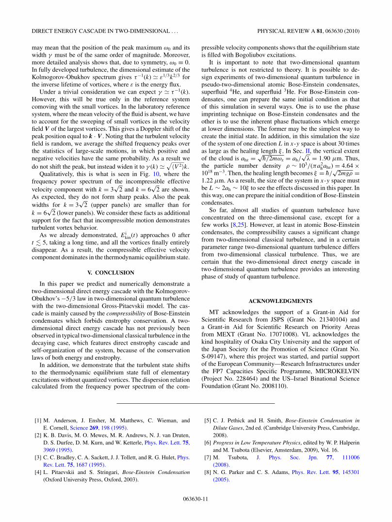
7. Frequency spectra of compressible and incompressiblevelocity components for different k and different g at later timemoments, shown in Figs. 8 and 10, respectively, with positionsof the maxima of the compressible frequency spectra ωmax(k)shown in Fig. 9 for different g and different moments oftime.

(b) (c)(a)

(e) (f)(d)

t=1 t=1 t=1

FIG. 4. (Color online) Log-log plots of the spectra of incompressible kinetic energy at earlier (upper panels) and later (lower panels)moments of time. Left panels: g = 1. Middle panels: g = 2. Right panels: g = 4.

063630-5

RYU NUMASATO, MAKOTO TSUBOTA, AND VICTOR S. L’VOV PHYSICAL REVIEW A 81, 063630 (2010)

10-3

10-2

10-1

100

101

1 10

3 k 2 /

N (

k)

k

1 10

k

1 10

k

t=40.0t=15.0

k-1

average(4200 t 4500)

t=40.0

t=15.0

average(1700 t 2000)

t=40.0

t=15.0

average(300 t 600)

k-1 k-1

(a) (b) (c)

(d) (e) (f)

10-3

10-2

10-1

100

101

10-3

10-2

10-1

100

101

10-3

10-2

10-1

100

10110-3

10-2

10-1

10-3

10-2

10-1

10-3

10-2

10-1

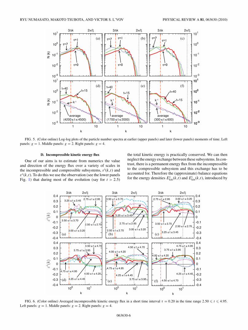
FIG. 5. (Color online) Log-log plots of the particle number spectra at earlier (upper panels) and later (lower panels) moments of time. Leftpanels: g = 1. Middle panels: g = 2. Right panels: g = 4.

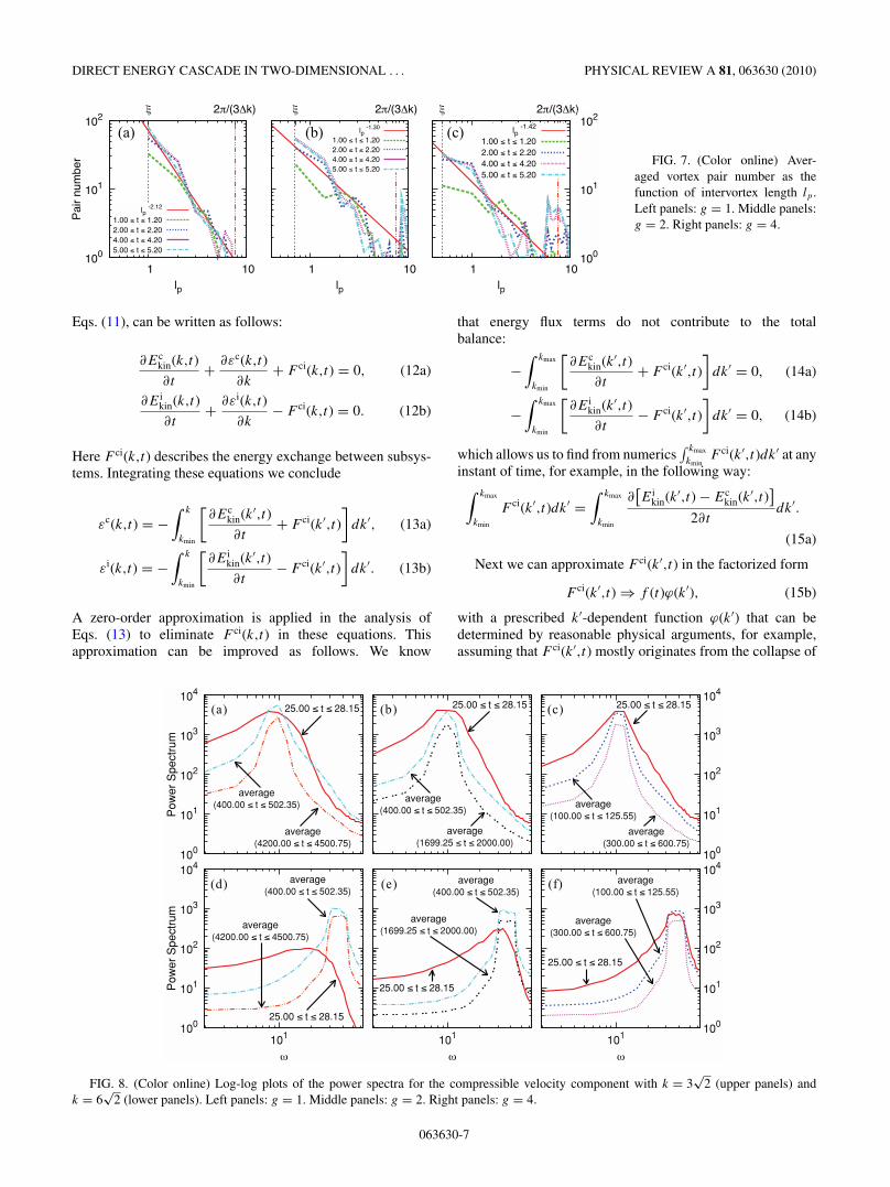
D. Incompressible kinetic energy flux

One of our aims is to estimate from numerics the valueand direction of the energy flux over a variety of scales inthe incompressible and compressible subsystems, εi(k,t) andεc(k,t). To do this we use the observation (see the lower panelsFig. 1) that during most of the evolution (say for t > 2.5)

the total kinetic energy is practically conserved. We can thenneglect the energy exchange between these subsystems. In con-trast, there is a permanent energy flux from the incompressibleto the compressible subsystem and this exchange has to beaccounted for. Therefore the (approximate) balance equationsfor the energy densities Ec

kin(k,t) and Eikin(k,t), introduced by

εi(k

)εi

(k)

(a) (b) (c)

(d) (e) (f)

FIG. 6. (Color online) Averaged incompressible kinetic energy flux in a short time interval τ = 0.20 in the time range 2.50 � t � 4.95.Left panels: g = 1. Middle panels: g = 2. Right panels: g = 4.

063630-6

DIRECT ENERGY CASCADE IN TWO-DIMENSIONAL . . . PHYSICAL REVIEW A 81, 063630 (2010)

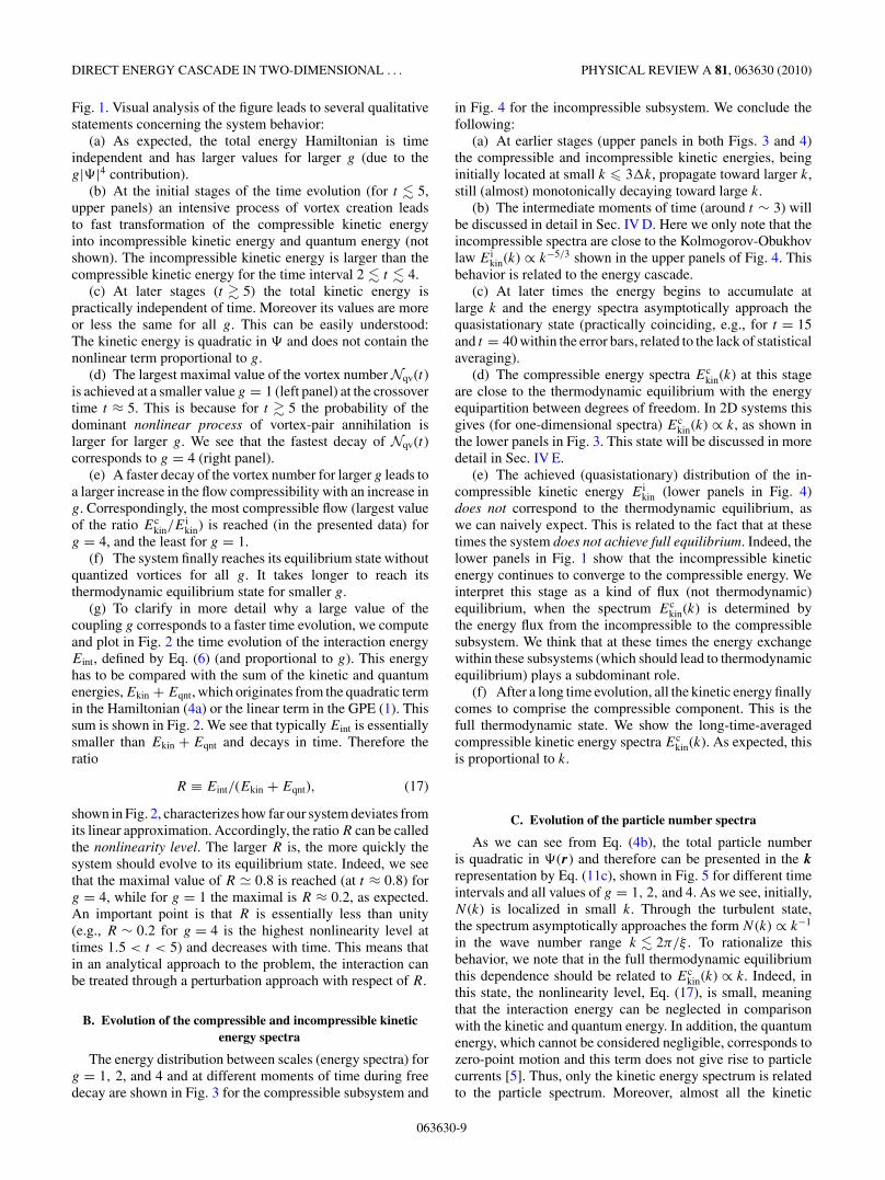
FIG. 7. (Color online) Aver-aged vortex pair number as thefunction of intervortex length lp .Left panels: g = 1. Middle panels:g = 2. Right panels: g = 4.

Eqs. (11), can be written as follows:

∂Eckin(k,t)

∂t+ ∂εc(k,t)

∂k+ F ci(k,t) = 0, (12a)

∂Eikin(k,t)

∂t+ ∂εi(k,t)

∂k− F ci(k,t) = 0. (12b)

Here F ci(k,t) describes the energy exchange between subsys-tems. Integrating these equations we conclude

εc(k,t) = −∫ k

kmin

[∂Ec

kin(k′,t)∂t

+ F ci(k′,t)]

dk′, (13a)

εi(k,t) = −∫ k

kmin

[∂Ei

kin(k′,t)∂t

− F ci(k′,t)]

dk′. (13b)

A zero-order approximation is applied in the analysis ofEqs. (13) to eliminate F ci(k,t) in these equations. Thisapproximation can be improved as follows. We know

that energy flux terms do not contribute to the totalbalance:

−∫ kmax

kmin

[∂Ec

kin(k′,t)∂t

+ F ci(k′,t)]

dk′ = 0, (14a)

−∫ kmax

kmin

[∂Ei

kin(k′,t)∂t

− F ci(k′,t)]

dk′ = 0, (14b)

which allows us to find from numerics∫ kmax

kminF ci(k′,t)dk′ at any

instant of time, for example, in the following way:∫ kmax

kmin

F ci(k′,t)dk′ =∫ kmax

kmin

∂[Ei

kin(k′,t) − Eckin(k′,t)

]2∂t

dk′.

(15a)

Next we can approximate F ci(k′,t) in the factorized form

F ci(k′,t) ⇒ f (t)ϕ(k′), (15b)

with a prescribed k′-dependent function ϕ(k′) that can bedetermined by reasonable physical arguments, for example,assuming that F ci(k′,t) mostly originates from the collapse of

100

101

102

103

104

1

Pow

er S

pect

rum

100

101

102

103

104

101

Pow

er S

pect

rum

101 101

25.00 t 28.15 25.00 t 28.1525.00 t 28.15

25.00 t 28.15

average(400.00 t 502.35)

25.00 t 28.15

25.00 t 28.15

average(400.00 t 502.35)

average(4200.00 t 4500.75)

average(4200.00 t 4500.75)

average(400.00 t 502.35)

average(400.00 t 502.35)

average(1699.25 t 2000.00)

average(1699.25 t 2000.00)

average(100.00 t 125.55)

average(100.00 t 125.55)

average(300.00 t 600.75)

average(300.00 t 600.75)

)c()b()a(

)f()e()d(

100

101

102

103

104

100

101

102

103

104

FIG. 8. (Color online) Log-log plots of the power spectra for the compressible velocity component with k = 3√

2 (upper panels) andk = 6

√2 (lower panels). Left panels: g = 1. Middle panels: g = 2. Right panels: g = 4.

063630-7

RYU NUMASATO, MAKOTO TSUBOTA, AND VICTOR S. L’VOV PHYSICAL REVIEW A 81, 063630 (2010)

100

101

102

1 10

c 2 /

max

k

1 10

c 2 /

k

1 10

c 2 /

k

2g2g 2g

ωmax =12gk2 +

14k4 ωmax =

12gk2 +

14k4 ωmax =

12gk2 +

14k4

12k2 1

2k2

12k2

: average(4200.00 t 4500.75)

: average(1699.25 t 2000.00)

: average(300.00 t 600.75)

(a) (b) (c)100

101

102

FIG. 9. (Color online) Position of the maximum frequency power spectra of the compressible velocity component for different wavevectors, averaged over a long time in the state of full thermodynamic equilibrium (full dots). Bogoliubov’s frequency spectrum ωmax(k),Eq. (21), and its large-k asymptotic ωmax(k) ∝ k2 are also shown. Left panel: g = 1. Middle panel: g = 2. Right panel: g = 4.

vortex pairs, and noting that the velocity around each vortexdecays like 1/r ′, and giving in the k′ representation an energyexchange proportional to k′ and Ei

kin(k′) ∝ k′|w(k′)|2. In ourcalculations we took ϕ(k′) ∝ k′3, or in the normalized form

ϕ(k′) = 4k′3/k4max. (15c)

Then from Eq. (15a) we find

f (t) ≈∫ kmax

kmin

∂[Ei

kin(k′,t) − Eckin(k′,t)

]2∂t

dk′. (15d)

Equations (15b), (15c), and (15d) can be substituted backinto Eqs. (13) to get an improved approximation for the flux.

Finally, we obtain the incompressible kinetic energy flux in aform with (15d):

εi(k,t) ≈ −∫ k

kmin

∂Eikin(k′,t)∂t

dk′ + f (t)

(k

kmax

)4

. (16)

Numerical results for the energy flux, obtained in this way, areshown in Fig. 6 and will be discussed later.

IV. DECAY OF 2D COMPRESSIBLE TURBULENCE

A. Free evolution of system energies and vortex number

Energy evolutions of the GP system, starting from thesame initial condition �(r,0), but with different values ofthe coupling constant, g = 1, g = 2, and g = 4, are shown in

100

101

102

103

104

1

Pow

er S

pect

rum

25.00 t 28.1537.80 t 40.95

25.00 t 28.1537.80 t 40.95

10-1

100

101

102

103

101

Pow

er S

pect

rum

25.00 t 28.1537.80 t 40.95

101

25.00 t 28.1537.80 t 40.95

101

25.00 t 28.1537.80 t 40.95

25.00 t 28.15

25.00 t 28.1525.00 t 28.15

25.00 t 28.15

37.80 t 40.95

37.80 t 40.95

37.80 t 40.95

37.80 t 40.95

37.80 t 40.9537.80 t 40.95

25.00 t 28.1525.00 t 28.15

(c)(b)(a)

(f)(e)(d)

100

101

102

103

104

10-1

100

101

102

103

FIG. 10. (Color online) Log-log plots of the power spectra for the incompressible velocity component with k = 3√

2 (upper panels) andk = 6

√2 (lower panels). Left panels: g = 1. Middle panels: g = 2. Right panels: g = 4.

063630-8

DIRECT ENERGY CASCADE IN TWO-DIMENSIONAL . . . PHYSICAL REVIEW A 81, 063630 (2010)

Fig. 1. Visual analysis of the figure leads to several qualitativestatements concerning the system behavior:

(a) As expected, the total energy Hamiltonian is timeindependent and has larger values for larger g (due to theg|�|4 contribution).

(b) At the initial stages of the time evolution (for t � 5,upper panels) an intensive process of vortex creation leadsto fast transformation of the compressible kinetic energyinto incompressible kinetic energy and quantum energy (notshown). The incompressible kinetic energy is larger than thecompressible kinetic energy for the time interval 2 � t � 4.

(c) At later stages (t � 5) the total kinetic energy ispractically independent of time. Moreover its values are moreor less the same for all g. This can be easily understood:The kinetic energy is quadratic in � and does not contain thenonlinear term proportional to g.

(d) The largest maximal value of the vortex number Nqv(t)is achieved at a smaller value g = 1 (left panel) at the crossovertime t ≈ 5. This is because for t � 5 the probability of thedominant nonlinear process of vortex-pair annihilation islarger for larger g. We see that the fastest decay of Nqv(t)corresponds to g = 4 (right panel).

(e) A faster decay of the vortex number for larger g leads toa larger increase in the flow compressibility with an increase ing. Correspondingly, the most compressible flow (largest valueof the ratio Ec

kin/Eikin) is reached (in the presented data) for

g = 4, and the least for g = 1.(f) The system finally reaches its equilibrium state without

quantized vortices for all g. It takes longer to reach itsthermodynamic equilibrium state for smaller g.

(g) To clarify in more detail why a large value of thecoupling g corresponds to a faster time evolution, we computeand plot in Fig. 2 the time evolution of the interaction energyEint, defined by Eq. (6) (and proportional to g). This energyhas to be compared with the sum of the kinetic and quantumenergies, Ekin + Eqnt, which originates from the quadratic termin the Hamiltonian (4a) or the linear term in the GPE (1). Thissum is shown in Fig. 2. We see that typically Eint is essentiallysmaller than Ekin + Eqnt and decays in time. Therefore theratio

R ≡ Eint/(Ekin + Eqnt), (17)

shown in Fig. 2, characterizes how far our system deviates fromits linear approximation. Accordingly, the ratio R can be calledthe nonlinearity level. The larger R is, the more quickly thesystem should evolve to its equilibrium state. Indeed, we seethat the maximal value of R � 0.8 is reached (at t ≈ 0.8) forg = 4, while for g = 1 the maximal is R ≈ 0.2, as expected.An important point is that R is essentially less than unity(e.g., R ∼ 0.2 for g = 4 is the highest nonlinearity level attimes 1.5 < t < 5) and decreases with time. This means thatin an analytical approach to the problem, the interaction canbe treated through a perturbation approach with respect of R.

B. Evolution of the compressible and incompressible kineticenergy spectra

The energy distribution between scales (energy spectra) forg = 1, 2, and 4 and at different moments of time during freedecay are shown in Fig. 3 for the compressible subsystem and

in Fig. 4 for the incompressible subsystem. We conclude thefollowing:

(a) At earlier stages (upper panels in both Figs. 3 and 4)the compressible and incompressible kinetic energies, beinginitially located at small k � 3�k, propagate toward larger k,still (almost) monotonically decaying toward large k.

(b) The intermediate moments of time (around t ∼ 3) willbe discussed in detail in Sec. IV D. Here we only note that theincompressible spectra are close to the Kolmogorov-Obukhovlaw Ei

kin(k) ∝ k−5/3 shown in the upper panels of Fig. 4. Thisbehavior is related to the energy cascade.

(c) At later times the energy begins to accumulate atlarge k and the energy spectra asymptotically approach thequasistationary state (practically coinciding, e.g., for t = 15and t = 40 within the error bars, related to the lack of statisticalaveraging).

(d) The compressible energy spectra Eckin(k) at this stage

are close to the thermodynamic equilibrium with the energyequipartition between degrees of freedom. In 2D systems thisgives (for one-dimensional spectra) Ec

kin(k) ∝ k, as shown inthe lower panels in Fig. 3. This state will be discussed in moredetail in Sec. IV E.

(e) The achieved (quasistationary) distribution of the in-compressible kinetic energy Ei

kin (lower panels in Fig. 4)does not correspond to the thermodynamic equilibrium, aswe can naively expect. This is related to the fact that at thesetimes the system does not achieve full equilibrium. Indeed, thelower panels in Fig. 1 show that the incompressible kineticenergy continues to converge to the compressible energy. Weinterpret this stage as a kind of flux (not thermodynamic)equilibrium, when the spectrum Ec

kin(k) is determined bythe energy flux from the incompressible to the compressiblesubsystem. We think that at these times the energy exchangewithin these subsystems (which should lead to thermodynamicequilibrium) plays a subdominant role.

(f) After a long time evolution, all the kinetic energy finallycomes to comprise the compressible component. This is thefull thermodynamic state. We show the long-time-averagedcompressible kinetic energy spectra Ec

kin(k). As expected, thisis proportional to k.

C. Evolution of the particle number spectra

As we can see from Eq. (4b), the total particle numberis quadratic in �(r) and therefore can be presented in the krepresentation by Eq. (11c), shown in Fig. 5 for different timeintervals and all values of g = 1, 2, and 4. As we see, initially,N (k) is localized in small k. Through the turbulent state,the spectrum asymptotically approaches the form N (k) ∝ k−1

in the wave number range k � 2π/ξ . To rationalize thisbehavior, we note that in the full thermodynamic equilibriumthis dependence should be related to Ec

kin(k) ∝ k. Indeed, inthis state, the nonlinearity level, Eq. (17), is small, meaningthat the interaction energy can be neglected in comparisonwith the kinetic and quantum energy. In addition, the quantumenergy, which cannot be considered negligible, corresponds tozero-point motion and this term does not give rise to particlecurrents [5]. Thus, only the kinetic energy spectrum is relatedto the particle spectrum. Moreover, almost all the kinetic

063630-9

RYU NUMASATO, MAKOTO TSUBOTA, AND VICTOR S. L’VOV PHYSICAL REVIEW A 81, 063630 (2010)

energy becomes the compressible component and there areno vortices, and as a result θ has no singularities and becomesof order unity. Thus the kinetic energy density can be estimatedusing a wave number k as follows:

Ekin � Eckin � 1

2ρ|∇θ |2 ∼ 12ρk2|θ |2 ∼ 1

2ρk2, (18)

which becomes in k space, using (11a) and (11c), 12 |w(k)|2 �

12k2|�(k)|2, as a result,

Eckin(k) � 1

2k2N (k). (19)

In this way, the two relations Eckin(k) ∝ k and N (k) ∝ k−1 hold

simultaneously. This relation is similar to the relation betweenenstrophy � and kinetic energy E in 2D classical fluids.

D. Observation of 2D direct energy cascade

Returning to the discussion of Figs. 1 and 3, we note thefollowing:

(a) The incompressible energy spectra at these times canbe interpreted as closed to the classical Kolmogorov-Obukhovdistribution Ei

kin(k) ∝ k−5/3, shown in the upper panels ofFig. 4.

(b) Bearing in mind that during the system evolution thekinetic energy clearly propagates from small k [where it wasinitially located in Ei

kin(k)] toward large k we conclude thatat some region of the system parameters we can observe a2D-direct energy cascade, which has previously been observedonly in 3D hydrodynamic systems.

(c) Numerical analysis of the incompressible kinetic en-ergy flux supports this explanation (b). Using Eq. (16), wecalculate the incompressible kinetic energy flux. Averageddata for a short time interval τ = 0.20 with five sets of data areshown in Fig. 6. The flux εi(k) takes positive values for 3�k �k � 2π/ξ at least for 2.50 � t � 4.95. This strongly supportsthe occurrence of a 2D direct energy cascade. Moreover, owingto the second term in Eq. (16), especially effective for highwave numbers, εi(k) tends to vanish at kmax.

(d) The Kolmogorov energy spectrum Eikin(k) ∝ k−5/3 was

previously observed in decaying 2D turbulence in the GPE[8]. However, this observation was interpreted in terms of theknown 2D turbulence inverse energy cascade, predicted byKraichnan [18]. We think that this interpretation is mistaken.In particular, if this interpretation is true, this spectrum has tobe followed by a k−3 spectrum for a direct enstrophy cascadeaccording to Kraichnan’s scenario. However, the authors ofRef. [8] “observe a k−6 dependence in this range”, instead ofa k−3 dependence.

(e) When the Kolmogorov-Obukhov spectrum is formed,a two-dimensional Richardson cascade can be seen. We canidentify the cores of the quantized vortices by finding thephase defects of the wave function. Then, we choose theshortest intervortex pair length lp for all vortices. In Fig. 7,the averaged vortex pair number Npair(lp) is shown and is pro-portional to l−n

p , where n depends on g and 1.30 � n � 2.12.This power law suggests a self-similar spatial structure. Fortwo-dimensional vortices, one of the most effective lengths,corresponding to the length of three-dimensional vortex ring,is the intervortex length. We conclude that Fig. 7 impliesthe following: First, vortex pairs with distances comparable

to 2π/(3�k) are created. Second, the vortex pair distanceprogressively decreases. Finally, when the vortex pair distancebecomes comparable to ξ , the pair is annihilated.

E. Frequency power spectra and types of motions

1. Compressible type of motion

Important information about types of motion can beextracted from the frequency power spectrum, which isthe Fourier transform of the different-time pair correlationfunction of the motion amplitude. For example, if an amplitudeA(t) oscillates with a particular frequency ω0, that is, A(t) =A0 exp(iω0t), then

J (τ ) ≡ 〈A(t + τ )A∗(t)〉 = A20 exp(iω0τ ),

giving

J (ω) =∫

J (τ ) exp(−iωτ )dτ ∝ δ(ω − ω0).

In other words, pure periodic motion with frequency ω0 has afrequency power spectrum with a very intensive peak of zerowidth at ω = ω0. It is easy to check that decaying oscillationsA(t) = A0 exp(−γ t + iω0t) have the power spectrum

J (ω) ∝ γ

(ω − ω0)2 + γ 2, (20)

that is, a peak at frequency ω0 and width γ , inverselyproportional to the lifetime of the motion.

We observed exactly this kind of frequency power spectrafor the compressible velocity component at later times, asshown in Fig. 8 for k = 3

√2 and k = 6

√2. As the system

evolves to the thermodynamic equilibrium state, the powerspectrum forms sharp peaks. This tendency is also seen in thefrequency power spectrum of the wave function � (not shown).We repeated this analysis for different k and in Fig. 9 we plotthe position of the maxima of the frequency power spectraof compressible motion, averaged over a long time intervalin the thermodynamic equilibrium state. Bearing in mind thatfor these periods the nonlinearity level R is very small (about0.04 for g = 4 and even smaller for g = 2 and 1), one canconsider these fluctuations as almost linear perturbations onthe background of the rest state. The eigenfrequencies of theseoscillations have been found by Bogoliubov [5] with the result

ωmax =√

12gk2 + 1

4k4, (21)

plotted in Fig. 9. The excellent agreement between thetheoretical and numerical results indicates that the observedthermodynamical fluctuation of the compressible velocitycomponent is indeed Bogoliubov’s elementary excitations.The relatively small, but finite width of the observed peakscharacterizes the finiteness of the lifetime of these fluctuations,caused by interaction of the fluctuations with different k-vectors.

2. Incompressible type of motion

What kind of frequency power spectrum can we expect forthe incompressible type of motion? To answer this we notethat an incompressible fluid exhibits vortex motions in whichthe lifetime and turnover time are of the same order. This

063630-10

DIRECT ENERGY CASCADE IN TWO-DIMENSIONAL . . . PHYSICAL REVIEW A 81, 063630 (2010)

may mean that the position of the peak maximum ω0 and itswidth γ must be of the same order of magnitude. Moreover,more detailed analysis shows that, due to symmetry, ω0 ≡ 0.In fully developed turbulence, the dimensional estimate of theKolmogorov-Obukhov spectrum gives τ−1(k) � ε1/3k2/3 forthe inverse lifetime of vortices, where ε is the energy flux.

Under a trivial consideration we can expect γ � τ−1(k).However, this will be true only in the reference systemcomoving with the small vortices. In the laboratory referencesystem, where the mean velocity of the fluid is absent, we haveto account for the sweeping of small vortices in the velocityfield V of the largest vortices. This gives a Doppler shift of thepeak position equal to k · V . Noting that the turbulent velocityfield is random, we average the shifted frequency peaks overthe statistics of large-scale motions, in which positive andnegative velocities have the same probability. As a result wedo not shift the peak, but instead widen it to γ (k) �

√〈V 2〉k.

Qualitatively, this is what is seen in Fig. 10, where thefrequency power spectrum of the incompressible effectivevelocity component with k = 3

√2 and k = 6

√2 are shown.

As expected, they do not form sharp peaks. Also the peakwidths for k = 3

√2 (upper panels) are smaller than for

k = 6√

2 (lower panels). We consider these facts as additionalsupport for the fact that incompressible motion demonstratesturbulent vortex behavior.

As we already demonstrated, Eikin(t) approaches 0 after

t � 5, taking a long time, and all the vortices finally entirelydisappear. As a result, the compressible effective velocitycomponent dominates in the thermodynamic equilibrium state.

V. CONCLUSION

In this paper we predict and numerically demonstrate atwo-dimensional direct energy cascade with the Kolmogorov-Obukhov’s −5/3 law in two-dimensional quantum turbulencewith the two-dimensional Gross-Pitaevskii model. The cas-cade is mainly caused by the compressibility of Bose-Einsteincondensates which forbids enstrophy conservation. A two-dimensional direct energy cascade has not previously beenobserved in typical two-dimensional classical turbulence in thedecaying case, which features direct enstrophy cascade andself-organization of the system, because of the conservationlaws of both energy and enstrophy.

In addition, we demonstrate that the turbulent state shiftsto the thermodynamic equilibrium state full of elementaryexcitations without quantized vortices. The dispersion relationcalculated from the frequency power spectrum of the com-

pressible velocity components shows that the equilibrium stateis filled with Bogoliubov excitations.

It is important to note that two-dimensional quantumturbulence is not restricted to theory. It is possible to de-sign experiments of two-dimensional quantum turbulence inpseudo-two-dimensional atomic Bose-Einstein condensates,superfluid 4He, and superfluid 3He. For Bose-Einstein con-densates, one can prepare the same initial condition as thatof this simulation in several ways. One is to use the phaseimprinting technique on Bose-Einstein condensates and theother is to use the inherent phase fluctuations which emergeat lower dimensions. The former may be the simplest way tocreate the initial state. In addition, in this simulation the sizeof the system of one direction L in x-y space is about 30 timesas large as the healing length ξ . In Sec. II, the vertical extentof the cloud is ahz = √

h/2mωz = ah/√

λ = 1.90 µm. Thus,the particle number density ρ ∼ 103/(πa2

hahz) = 4.64 ×1018 m−3. Then, the healing length becomes ξ = h/

√2mgρ =

1.22 µm. As a result, the size of the system in x-y space mustbe L ∼ 2ah ∼ 10ξ to see the effects discussed in this paper. Inthis way, one can prepare the initial condition of Bose-Einsteincondensates.

So far, almost all studies of quantum turbulence haveconcentrated on the three-dimensional case, except for afew works [8,25]. However, at least in atomic Bose-Einsteincondensates, the compressibility causes a significant changefrom two-dimensional classical turbulence, and in a certainparameter range two-dimensional quantum turbulence differsfrom two-dimensional classical turbulence. Thus, we arecertain that the two-dimensional direct energy cascade intwo-dimensional quantum turbulence provides an interestingphase of study of quantum turbulence.

ACKNOWLEDGMENTS

MT acknowledges the support of a Grant-in Aid forScientific Research from JSPS (Grant No. 21340104) anda Grant-in Aid for Scientific Research on Priority Areasfrom MEXT (Grant No. 17071008). VL acknowledges thekind hospitality of Osaka City University and the support ofthe Japan Society for the Promotion of Science (Grant No.S-09147), where this project was started, and partial supportof the European Community—Research Infrastructures underthe FP7 Capacities Specific Programme, MICROKELVIN(Project No. 228464) and the US–Israel Binational ScienceFoundation (Grant No. 2008110).

[1] M. Anderson, J. Ensher, M. Matthews, C. Wieman, andE. Cornell, Science 269, 198 (1995).

[2] K. B. Davis, M. O. Mewes, M. R. Andrews, N. J. van Druten,D. S. Durfee, D. M. Kurn, and W. Ketterle, Phys. Rev. Lett. 75,3969 (1995).

[3] C. C. Bradley, C. A. Sackett, J. J. Tollett, and R. G. Hulet, Phys.Rev. Lett. 75, 1687 (1995).

[4] L. Pitaevskii and S. Stringari, Bose-Einstein Condensation(Oxford University Press, Oxford, 2003).

[5] C. J. Pethick and H. Smith, Bose-Einstein Condensation inDilute Gases, 2nd ed. (Cambridge University Press, Cambridge,2008).

[6] Progress in Low Temperature Physics, edited by W. P. Halperinand M. Tsubota (Elsevier, Amsterdam, 2009), Vol. 16.

[7] M. Tsubota, J. Phys. Soc. Jpn. 77, 111006(2008).

[8] N. G. Parker and C. S. Adams, Phys. Rev. Lett. 95, 145301(2005).

063630-11

RYU NUMASATO, MAKOTO TSUBOTA, AND VICTOR S. L’VOV PHYSICAL REVIEW A 81, 063630 (2010)

[9] M. Kobayashi and M. Tsubota, Phys. Rev. Lett. 94, 065302(2005); J. Phys. Soc. Jpn. 74, 3248 (2005).

[10] M. Kobayashi and M. Tsubota, Phys. Rev. Lett. 97, 145301(2006).

[11] V. B. Eltsov, A. I. Golov, R. de Graaf, R. Hanninen, M. Krusius,V. S. L’vov, and R. E. Solntsev, Phys. Rev. Lett. 99, 265301(2007).

[12] P. M. Walmsley, A. I. Golov, H. E. Hall, A. A. Levchenko, andW. F. Vinen, Phys. Rev. Lett. 99, 265302 (2007).

[13] V. B. Eltsov, R. de Graaf, R. Hanninen, M. Krusius, R. E.Solntsev, V. S. L’vov, A. I. Golov, and P. M. Walmsley,in Progress in Low Temperature Physics, edited by W. P.Halperin and M. Tsubota (Elsevier, Amsterdam, 2009),Vol. 16, p. 46.

[14] C. Nore, M. Abid, and M. E. Brachet, Phys. Rev. Lett. 78, 3896(1997); Phys. Fluids 9, 2644 (1997).

[15] M. Abid, C. Huepe, S. Metens, C. Nore, C. Pham,L. Tuckerman, and M. Brachet, Fluid Dyn. Res. 33, 509 (2003).

[16] J. Maurer and P. Tabeling, Europhys. Lett. 43, 29(1998).

[17] T. Araki, M. Tsubota, and S. K. Nemirovskii, Phys. Rev. Lett.89, 145301 (2002).

[18] R. H. Kraichnan, Phys. Fluids 10, 1417 (1967).[19] P. Tabeling, Phys. Rep. 362, 1 (2002).[20] J. R. Herring and J. C. McWilliams, J. Fluid Mech. 153, 229

(1985).[21] G. Boffetta, A. Celani, and M. Vergassola, Phys. Rev. E 61, R29

(2000).[22] J.-P. Laval, B. Dubrulle, and S. V. Nazarenko, J. Comput. Phys.

196, 184 (2004).[23] R. Numasato and M. Tsubota, J. Low Temp. Phys. 158, 415

(2010).[24] K. Kasamatsu, M. Tsubota, and M. Ueda, Phys. Rev. A 67,

033610 (2003).[25] T.-L. Horng, C.-H. Hsueh, S.-W. Su, Y.-M. Kao, and S.-C. Gou,

Phys. Rev. A 80, 023618 (2009).

063630-12