Seediscussions,stats,andauthorprofilesforthispublicationat:https://www.researchgate.net/publication/280625651

DirectComparisonofSingle-SpecimenClampedSE(T)TestMethodsonX100LinePipeSteel

ConferencePaper·October2014

DOI:10.1115/IPC2014-33695

READS

31

2authors:

TimothyS.Weeks

NationalInstituteofStandardsandTechnolo…

10PUBLICATIONS23CITATIONS

SEEPROFILE

EnricoLucon

NationalInstituteofStandardsandTechnolo…

102PUBLICATIONS779CITATIONS

SEEPROFILE

Availablefrom:TimothyS.Weeks

Retrievedon:14April2016

Proceedings of the 10th International Pipeline Conference IPC2014

September 29-October 3, 2014, Calgary, Alberta, Canada

IPC2014-33695

DIRECT COMPARISON OF SINGLE-SPECIMEN CLAMPED SE(T) TEST METHODS ON X100 LINE PIPE STEEL

Timothy S. Weeks and Enrico Lucon† National Institute of Standards and

Technology Boulder, CO, USA

† Protiro, Inc. contractor to NIST

ABSTRACT

The clamped single edge-notched tension (SE(T)) specimen has been widely used in a single-specimen testing scheme to generate fracture resistance curves for high strength line-pipe steels. The SE(T) specimen with appropriate notch geometry is a low-constraint specimen designed to reduce conservatism in the measurement of fracture toughness. The crack driving force is taken as either the J-integral or crack tip opening displacement (CTOD); it is generally accepted that the two parameters are interchangeable and equivalent using a simple closed form solution. However, the assumption that they are interchangeable, and to what extent, hasn’t been previously investigated experimentally on the same SE(T) specimen. This paper presents multiple test methods that were simultaneously employed on the same SE(T) specimens. The instrumentation includes: clip-gauges to measure surface crack mouth opening displacements (CMOD) and CTOD by the double-clip-gauge method; strain-gage arrays for direct J-integral measurements; and direct-current potential-drop (DCPD) instrumentation for supplementary crack size measurement. A direct comparison of ductile crack-growth resistance curves generated using J-integral and CTOD is presented here where each represents a different experimental and analytical approach. The two methods are in reasonable agreement over a narrow range of crack growth, differing slightly at initiation and diverging with increasing crack growth. Analysis of the supplementary instrumentation (i.e., strain gages, extensometers and DCPD) will be provided in a future publication. INTRODUCTION Commonly used fracture mechanics test standards, such as ASTM E1820-11e2 [1], BS 7448-1 [2] and ISO 12135 [3], mainly address the measurement of fracture toughness by use

of high constraint laboratory specimens, such as compact tension C(T), single edge-notched bend SE(B), and disk-shaped compact tension DC(T). In its most recent revision, ASTM E1820-11e2 [1] added an appendix to support low-constraint shallow cracked SE(B) specimens. High-constraint (deep-cracked) specimens provide more conservative toughness values than low-constraint (shallow-cracked) specimens; however, in general, bend specimens provide higher constraint than tension specimens at the same crack depth. The lower stress-triaxiality at the crack tip in SE(T) specimens delays crack initiation and enhances crack growth resistance. The effects of increasing triaxiality are observed when comparing SE(T) specimens with shallow cracks (a/W ≈ 0.25) and deep cracks (a/W ≈ 0.45, [4] a/W ≈ 0.5 [5, 6]). However, the parametric influence on toughness values for the purpose of a reasonable comparison between specimen geometry, flaw geometry and loading mode remains elusive sans standardized testing procedures. Despite the lack of a consensus testing standard, considerable research has been done on the SE(T) fracture specimen [4-19] and there are three recommended practices currently in use. The recommended practices are used to evaluate ductile crack propagation: the multi-specimen test [20], and two single-specimen tests [21, 22]. Some recent results have been published comparing the multi-specimen method to a single-specimen method [10], while this research is aimed at comparing the two single-specimen methods. The two single-specimen methods will be referred to as the J-R method and the CTOD-R method. The J-R and CTOD-R methods sourced from the recommended practices published by CanmetMATERIALS, Natural Resources Canada [21] and ExxonMobil Upstream Research Company [22], respectively, define the specimen geometry, notch geometry, crack geometry,

1 Contribution of an agency of the US government, ASME disclaims all interest in the US government’s contributions.

general experimental setup, loading profile and analysis of the data. Furthermore, in this study we employed both test methods simultaneously on a common specimen during the conduct of a test. Normalizing critical test parameters (i.e., material, geometry, instrumentation, environment, and operator) between the methods is the principal enabler for direct comparison of the two methods. Both methods use the technique of CMOD unloading compliance (UC) (ΔCMOD/ΔForce), which is familiar in standardized single-specimen toughness testing. The force is measured directly during each of the unloading cycles, and the crack extension is calculated from the CMOD UC expressions according to the recommended practices cited and detailed in this paper. The J-R method evaluates the J-integral at each increment of crack extension, while the CTOD-R method evaluates the CTOD (δ). The fracture resistance is then characterized by the J-R or CTOD-R curves (J or δ as a function of Δa) in the absence of brittle fracture. The experimental design, instrumentation, setup, and test procedure details were published previously [23]. Pertinent details of the test methods to support the analysis methods, as well as a comprehensive comparison of the results obtained by each method, will be presented here. Analysis of the supplementary instrumentation as described in the original paper (i.e., strain gages, extensometers and DCPD) will be provided in a future publication. Comparison between the two methods requires but does not assume that the instrumentation used for each will accurately measure the same physical and mechanical attributes of the specimen under applied force. The Instrumentation section here will briefly describe the instrumentation and the geometric relationships between the instrumentation required by the two methods. The J-R Analysis and CTOD-R Analysis sections detail the measurements and equations used to generate J-R and CTOD-R curves for each specimen. The Results and Comparison section presents the J-R and CTOD-R curves for each specimen. The Discussion section describes the complexities encountered in this research, and finally some observations of the critical parameters influencing the results conclude this paper. EXPERIMENTAL DESIGN AND MATERIAL Evaluating the J-integral in the present research requires direct measurement of the CMOD. The direct measurement of CMOD is accomplished by use of integral knife-edges machined into the notch mouth. The CMOD can also be inferred by use of a double-clip-gauge method. Difficulties

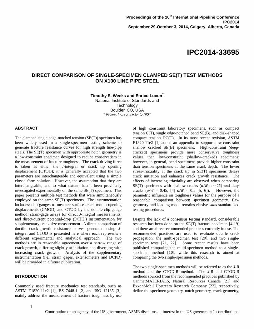
with use of these techniques will be discussed later. The only data required for J-integral analysis are force and CMOD. For this study, the double-clip-gauge method is also used to calculate the CTOD of the advancing crack. This is made possible by use of a double-clip-gauge mounting fixture attached to the surface of the specimen where the knife-edges are at different distances from the specimen surface. The double-clip-gauge mounting fixture ensures that the clip-gauge measurement locations are coplanar with each other. The data required for the CTOD-R method are the forces, and displacements measured by clip-gauge V1 and clip-gauge V2. The clip-gauge details will be provided in the Instrumentation section. Specimen blanks were cut in the axial direction from a section of 914, mm diameter 19.1 mm wall thickness, X100 UOE pipe straddling the 3 o’clock position. The tensile tests were performed at CanmetMATERIALS, using round bars cut from the four corners of the section of pipe used for the SE(T) tests. Measured values of yield and ultimate strengths at room temperature were 745±8 MPa and 835±11 MPa (all reported error bounds are ± one standard deviation) [24]. SPECIMEN GEOMETRY Square cross-section specimens (B×B, B=W) were used. The nominal thickness of each specimen was 17.5 mm. The initial crack size to thickness ratio (a0/W) was set at 0.4 to match the crack size used by Tyson and Gianetto [24] in a J-R round-robin testing program. Three different notch root-radii were evaluated and the results are presented here. The notches and integral knife-edges were machined using a continuous-wire electric-discharge machining (EDM) method. One specimen had a 7 mm deep notch machined using a Ø0.1 mm wire, and two specimens had 7 mm notches machined using a Ø0.25 mm wire. The final two specimens were initially notched to 5 mm with the Ø0.25 mm wire, but were then fatigue pre-cracked to 7 mm to obtain the prescribed a0/W ratio of 0.4 for all specimens tested. The resulting notch root-radii were 0.152 mm, 0.051 mm, and 0.0 mm, respectively. The notch geometries and integral knife-edge details are illustrated in Figure 1. Both sides of the specimens were side-grooved to 0.075B for a reduced total thickness of 0.85B. The details of the side grooves are shown in Figure 2. The net section thickness (BN) was 14.875 mm. The double-clip-gauge mounting fixture was mounted to the front face of the specimen using tapped holes on either side of the notch. The details and dimensions of the holes as recommended by [22] are shown in Figure 3.

2 Contribution of an agency of the US government, ASME disclaims all interest in the US government’s contributions.

The length of each specimen was 315 mm (18W), which allowed for a grip-to-grip separation (H) of 175 mm (10W) and a grip length of 70 mm (4W) on each end of the specimen.

Figure 1. Notch geometry and integral knife-edge details for (a) 0.1 mm wire EDM, (b) 0.25 mm wire EDM and (c) fatigue pre-cracked specimens (all linear dimensions in mm).

Figure 2. Details of the side grooves for each specimen. Total reduction in thickness is 0.15B (all linear dimensions in mm).

Figure 3. Threaded-hole details for the double-clip-gauge mounting fixture (all linear dimensions in mm).

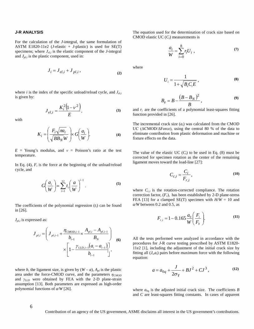
INSTRUMENTATION Identical clip-gauges were used on the front face of the specimens to measure CMOD and calculate CTOD. The opening displacements associated with the double-clip-gauge mounting fixture are designated as the z=2 mm (V1) and z=8 mm (V2) measurements, where z is the distance of the clip-gauge knife-edge from the surface of the specimen. The double-clip-gauge mounting fixture was notched, permitting the use of a third clip-gauge that was integrally attached at the specimen surface: z=0. The double-clip-gauge mounting fixture was installed so that the CMOD integral knife-edge, the V1 knife-edge, and the V2 knife-edge were coplanar and laterally spaced by approximately 12.5 mm. Details of the double-clip-gauge mounting fixture are shown in Figure 4. The three clip-gauges were full-bridge ring-style gages as shown in Figure 5. The beams of the original equipment were replaced with yttria-stabilized zirconia ceramic in order to electrically isolate the extensometers from the specimen. The ceramic beam replacements replicated the original equipment and followed the recommendations of ASTM E399-12e1 [25] and ASTM E1820-11e2 [1]. The clip-gauges were calibrated in the opening mode with the zero point set to match the initial knife-edge opening of each specimen (2.6 mm).

3 Contribution of an agency of the US government, ASME disclaims all interest in the US government’s contributions.

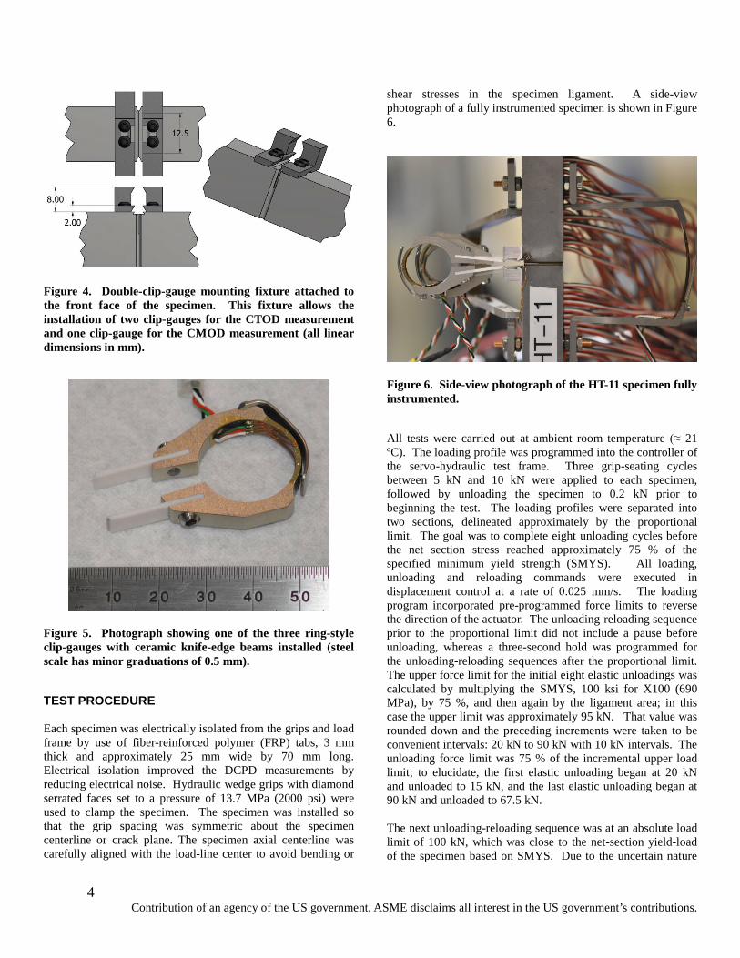
Figure 4. Double-clip-gauge mounting fixture attached to the front face of the specimen. This fixture allows the installation of two clip-gauges for the CTOD measurement and one clip-gauge for the CMOD measurement (all linear dimensions in mm).

Figure 5. Photograph showing one of the three ring-style clip-gauges with ceramic knife-edge beams installed (steel scale has minor graduations of 0.5 mm).

TEST PROCEDURE Each specimen was electrically isolated from the grips and load frame by use of fiber-reinforced polymer (FRP) tabs, 3 mm thick and approximately 25 mm wide by 70 mm long. Electrical isolation improved the DCPD measurements by reducing electrical noise. Hydraulic wedge grips with diamond serrated faces set to a pressure of 13.7 MPa (2000 psi) were used to clamp the specimen. The specimen was installed so that the grip spacing was symmetric about the specimen centerline or crack plane. The specimen axial centerline was carefully aligned with the load-line center to avoid bending or

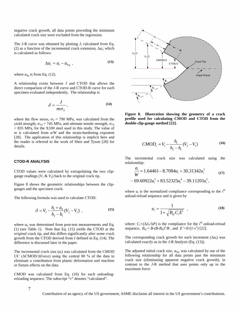
shear stresses in the specimen ligament. A side-view photograph of a fully instrumented specimen is shown in Figure 6.

Figure 6. Side-view photograph of the HT-11 specimen fully instrumented.

All tests were carried out at ambient room temperature (≈ 21 ºC). The loading profile was programmed into the controller of the servo-hydraulic test frame. Three grip-seating cycles between 5 kN and 10 kN were applied to each specimen, followed by unloading the specimen to 0.2 kN prior to beginning the test. The loading profiles were separated into two sections, delineated approximately by the proportional limit. The goal was to complete eight unloading cycles before the net section stress reached approximately 75 % of the specified minimum yield strength (SMYS). All loading, unloading and reloading commands were executed in displacement control at a rate of 0.025 mm/s. The loading program incorporated pre-programmed force limits to reverse the direction of the actuator. The unloading-reloading sequence prior to the proportional limit did not include a pause before unloading, whereas a three-second hold was programmed for the unloading-reloading sequences after the proportional limit. The upper force limit for the initial eight elastic unloadings was calculated by multiplying the SMYS, 100 ksi for X100 (690 MPa), by 75 %, and then again by the ligament area; in this case the upper limit was approximately 95 kN. That value was rounded down and the preceding increments were taken to be convenient intervals: 20 kN to 90 kN with 10 kN intervals. The unloading force limit was 75 % of the incremental upper load limit; to elucidate, the first elastic unloading began at 20 kN and unloaded to 15 kN, and the last elastic unloading began at 90 kN and unloaded to 67.5 kN. The next unloading-reloading sequence was at an absolute load limit of 100 kN, which was close to the net-section yield-load of the specimen based on SMYS. Due to the uncertain nature

4 Contribution of an agency of the US government, ASME disclaims all interest in the US government’s contributions.

of the yielding event and low slope of the post-yield Force-CMOD data, the operator had the option of interrupting this loading cycle and manually initiating the next sequence if it appeared that the pre-programmed increment would have lost data in the transition. The next section of the test, at loads above 100 kN, involved unloading/reloading cycles in the plastic range, where the specimen was also unloaded and reloaded in displacement-control at a rate of 0.025 mm/s. The limits defining the start and stop of each unload/reload cycle used the CMOD signal as a limit; a software loop was programmed to iterate the entire process. Beginning at the incremental load maximum (Pi

Max) of the current (ith) loading segment, specimens were held in displacement control for three seconds prior to unloading to a load 20 kN lower than Pi

Max and then reloaded by 18 kN. As an example, the first plastic loading increment P1

Max was scheduled at 100 kN; therefore, the actuator displacement was increased until 100 kN load was attained. At that point, the displacement was held for three seconds, and the specimen was then unloaded to 80 kN (P1

Max - 20 kN). The specimen was then reloaded by 18 kN (to 98 kN). Reloading the specimen by 18 kN ensured that the specimen was reloaded nominally elastically. Deformation was then continued until the CMOD had increased by a relative 0.15 mm. When the CMOD increment was reached, a new Pi

Max value was defined (based on the load achieved at the end of the increment) and the loop was iterated. A schematic view of this control method is shown in Figure 7. The CMOD increment effectively defines the number of unloadings in the plastic portion of the test, with a goal of acquiring 8 to 10 UC measurements prior to the specimen attaining a maximum in the applied force. The test continued past the maximum force and was terminated when the CMOD reached 3.5 mm. After each test the specimens were placed in a furnace at a temperature of 300 °C for approximately 30 minutes to heat-tint the exposed crack surfaces. Crack surfaces were liberated by brittle fracture in bending by use of liquid nitrogen. Fractographs were taken of both sides of each fracture surface. The fractographs were analyzed by use of criteria provided in the ASTM E1820-11e2 [1] standard as well as the CTOD-R recommended practice [22]. Each specimen was analyzed; the comparison of results presented here is limited to the analyses required by each of the recommended practices.

Figure 7. Schematic plot of the control method used after the proportional limit of the specimen. Each unloading-reloading cycle was done in displacement-control; the top plot shows the displacement vs. time of an unload-reload and unload cycle with a typical resulting load vs. CMOD plot shown in the bottom plot.

POST-TEST CRACK SIZE MEASUREMENTS Measurement methods to obtain the initial crack sizes, a0, are described in several sources and are common practices [1-3, 20, 22]. The measured crack sizes in this study are presented in Table 1. The values of a0 represent the average of the nine measurements and were determined according to the following relation:

( ) 8/2/8

20

90

100

++= ∑

=i

iaaaa . (1)

The same method and calculation is performed to determine the final crack sizes, af, and Δap is calculated as Δap=af - a0.

5 Contribution of an agency of the US government, ASME disclaims all interest in the US government’s contributions.

J-R ANALYSIS For the calculation of the J-integral, the same formulation of ASTM E1820-11e2 (J-elastic + J-plastic) is used for SE(T) specimens; where Jel,i is the elastic component of the J-integral and Jpl,i is the plastic component, used in:

iplieli JJJ ,, += ,

(2)

where i is the index of the specific unload/reload cycle, and Jel,i is given by:

( )E

KJ iiel

22

,1 ν−

= , (3)

with

×

=

WaG

WBBaF

K i

N

iii

π,

(4)

E = Young’s modulus, and ν = Poisson’s ratio at the test temperature. In Eq. (4), Fi is the force at the beginning of the unload/reload cycle, and

∑=

−

=

12

1

1

i

i

ii

Wat

WaG . (5)

The coefficients of the polynomial regression (ti) can be found in [26]. Jpl,i is expressed as:

−×+= −

−

−−

N

iplipl

i

iCMODiplipl B

AAb

JJ 1,,

1

1,1,,

η

( )

−−×

−

−−

1

11,1i

iiiLLD

baaγ

,

(6)

where b, the ligament size, is given by (W – a), Apl is the plastic area under the force-CMOD curve, and the parameters ηCMOD and γLLD were obtained by FEA with the 2-D plane-strain assumption [13]. Both parameters are expressed as high-order polynomial functions of a/W [26].

The equation used for the determination of crack size based on CMOD elastic UC (Ci) measurements is

∑=

=8

0iii

i UrWa , (7)

where

ECBU

iei +=

11

, (8)

( )BBBBB N

e

2−−= , (9)

and ri are the coefficients of a polynomial least-squares fitting function provided in [26]. The incremental crack size (ai) was calculated from the CMOD UC (ΔCMOD/ΔForce), using the central 80 % of the data to eliminate contribution from plastic deformation and machine or fixture effects on the data. The value of the elastic UC (Ci) to be used in Eq. (8) must be corrected for specimen rotation as the center of the remaining ligament moves toward the load-line [27]:

ir

iic F

CC,

, = , (10)

where Cc,i is the rotation-corrected compliance. The rotation correction factor, (Fr), has been established by 2-D plane-stress FEA [13] for a clamped SE(T) specimen with H/W = 10 and a/W between 0.2 and 0.5, as

−=

Y

iir F

FWaF 0

, 165.01 . (11)

All the tests performed were analyzed in accordance with the procedures for J-R curve testing prescribed by ASTM E1820-11e2 [1], including the adjustment of the initial crack size by fitting all (Ji,ai) pairs before maximum force with the following equation:

320 2

CJBJJaaY

q +++=σ

, (12)

where a0q is the adjusted initial crack size. The coefficients B and C are least-squares fitting constants. In cases of apparent

6 Contribution of an agency of the US government, ASME disclaims all interest in the US government’s contributions.

negative crack growth, all data points preceding the minimum calculated crack size were excluded from the regression. The J-R curve was obtained by plotting Ji calculated from Eq. (2) as a function of the incremental crack extension, Δai; which is calculated as follows:

qii aaa 0−=∆ , (13)

where a0q is from Eq. (12). A relationship exists between J and CTOD that allows the direct comparison of the J-R curve and CTOD-R curve for each specimen evaluated independently. The relationship is

YmJσ

δ = , (14)

where the flow stress, σY = 790 MPa, was calculated from the yield strength, σYS = 745 MPa, and ultimate tensile strength, σTS = 835 MPa, for the X100 steel used in this study. The value of m is calculated from a/W and the strain-hardening exponent [28]. The application of this relationship is implicit here and the reader is referred to the work of Shen and Tyson [28] for details. CTOD-R ANALYSIS CTOD values were calculated by extrapolating the two clip-gauge readings (V1 & V2) back to the original crack tip.

Figure 8 shows the geometric relationships between the clip-gauges and the specimen crack. The following formula was used to calculate CTOD:

)( 1212

011 VV

hhahV −

−+

−=δ , (15)

where a0 was determined from post-test measurements and Eq. (1) (see Table 1). Note that Eq. (15) yields the CTOD at the original crack tip, and this differs significantly after some crack growth from the CTOD derived from J defined in Eq. (14). The difference is discussed later in the paper. The incremental crack size (ai) was calculated from the CMOD UC (ΔCMOD/ΔForce) using the central 80 % of the data to eliminate a contribution from plastic deformation and machine or fixture effects on the data. CMOD was calculated from Eq. (16) for each unloading-reloading sequence. The subscript “c” denotes “calculated”.

Figure 8. Illustration showing the geometry of a crack profile used for calculating CMOD and CTOD from the double-clip-gauge method [22].

)( 1212

11 VV

hhhVCMODc −−

−= (16)

The incremental crack size was calculated using the relationship:

231342.307084.864461.1 iii uu

Wa

+−= 543 11201.3952325.8360922.69 iii uuu −+− ,

(17)

where ui is the normalized compliance corresponding to the ith unload-reload sequence and is given by

ECBu

iefi ′+=

11 , (18)

where: Ci=(Δδc/ΔP) is the compliance for the ith unload-reload sequence, Bef = B-(B-BN)2/B , and E’=E/(1-ν2) [22]. The corresponding crack growth for each increment (Δai) was calculated exactly as in the J-R Analysis (Eq. (13)). The adjusted initial crack size, a0q, was calculated by use of the following relationship for all data points past the minimum crack size (eliminating apparent negative crack growth), in contrast to the J-R method that uses points only up to the maximum force:

7 Contribution of an agency of the US government, ASME disclaims all interest in the US government’s contributions.

32

210 4.1

δδδδ CCaa q +++= . (19)

The CTOD-R curve was obtained by plotting δi as a function of the corresponding crack growth, Δai. The equation used for fitting in the CTOD-R method is:

𝛿𝛿 = 𝛼𝛼(∆𝑎𝑎)𝜂𝜂. (20)

To determine the fitting coefficients, α and η, of Eq. (20), all data from 0.5 mm up to the final measured crack growth value were fitted. RESULTS AND COMPARISON Measuring crack size is critical to the analysis of J-R or CTOD-R. Initial crack size as measured from post-test fractographs is required by the CTOD-R method to be used in Eq. (15). Comparing the average measured initial crack size, a0, to the adjusted initial crack size, a0q, is one of the qualifying tests used to validate the data in the CTOD-R analysis. The adjusted initial crack size is determined by plotting δi-ai data pairs and finding the minimum value of ai, and then fitting the data beyond that minimum, which effectively ignores apparent negative crack growth.

A similar comparison is expected in the J-R analysis; however, validity requirements have not been established. Furthermore, post-test measurement of the initial crack size is not required by the J-R method for use in the calculations. The adjusted initial crack size is determined by plotting Ji-ai data pairs and finding the minimum value of ai, and then fitting the data beyond that minimum, which effectively ignores apparent negative crack growth.

As previously mentioned separately in the J-R Analysis and CTOD-R Analysis sections, there is a significant difference between the fitting procedures used to determine the adjusted initial crack size. That is, the data pairs used in the J-R method end with the maximum force, whereas the CTOD-R method uses all data pairs up to the final crack size. Table 1 provides the measured initial crack sizes, a0, as well as the calculated a0q for each specimen determined by both analysis methods. Table 1 also provides the measured final crack sizes, af, the calculated final crack sizes for each specimen determined by both analysis methods, af,J and af,δ respectively, as well as the measured and calculated crack extensions. The final crack sizes, af,J and af,δ, were calculated from Eq. (7) and Eq. (17), respectively, where i corresponds to the final UC measurement. Specimen HT-11 has two values listed for each of the estimates by the CTOD-R method; these

values represent original and corrected values. Details of the correction are given in the Discussion section.

Table 1. Measured values of initial and final crack sizes from post-test fractographs including values calculated from the two recommended practices.

Specimen ID

Measured a0 mm

Calculated a0q (J-R) mm

Calculated a0q (CTOD-R)

mm HT-105-10 6.98 7.02 7.17 HT-105-11 6.98 6.89 8.27*/7.52* HT-105-12 6.74 7.05 7.23 HT-105-13 7.11 7.19 7.45 HT-105-14 7.25 7.25 7.34 Measured af

mm Calculated af,J

(J-R) mm

Calculated af,δ (CTOD-R)

mm HT-105-10 11.20 11.04 11.66 HT-105-11 10.31 10.32 11.23/11.09 HT-105-12 11.23 11.26 12.14 HT-105-13 11.55 11.61 12.50 HT-105-14 11.61 11.57 11.96 Measured

Δap mm

Calculated Δap (J-R) mm

Calculated Δap (CTOD-R)

mm HT-105-10 4.22 4.02 4.49 HT-105-11 3.33 3.43 2.96/3.57 HT-105-12 4.49 4.21 4.91 HT-105-13 4.44 4.42 5.05 HT-105-14 4.36 4.32 4.62 * Not a valid calculation based on discontinuous fitting

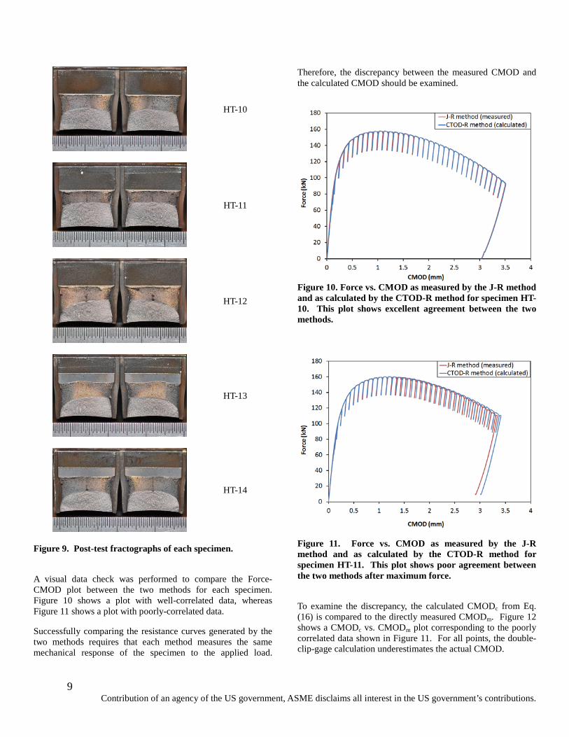
Post-test fractographs for each specimen are shown in Figure 9. Initial and final crack sizes were determined with image analysis software. Crack paths remained normal to the applied force in every specimen. To successfully compare the two approaches to fracture toughness, several methods of validating the data were applied. First, the CTOD-R method has validity requirements based on crack size measurements. Validity requirements for the CTOD-R method were met for all specimens except for specimen HT-11.

8 Contribution of an agency of the US government, ASME disclaims all interest in the US government’s contributions.

HT-10

HT-11

HT-12

HT-13

HT-14

Figure 9. Post-test fractographs of each specimen.

A visual data check was performed to compare the Force-CMOD plot between the two methods for each specimen. Figure 10 shows a plot with well-correlated data, whereas Figure 11 shows a plot with poorly-correlated data.

Successfully comparing the resistance curves generated by the two methods requires that each method measures the same mechanical response of the specimen to the applied load.

Therefore, the discrepancy between the measured CMOD and the calculated CMOD should be examined.

Figure 10. Force vs. CMOD as measured by the J-R method and as calculated by the CTOD-R method for specimen HT-10. This plot shows excellent agreement between the two methods.

Figure 11. Force vs. CMOD as measured by the J-R method and as calculated by the CTOD-R method for specimen HT-11. This plot shows poor agreement between the two methods after maximum force.

To examine the discrepancy, the calculated CMODc from Eq. (16) is compared to the directly measured CMODm. Figure 12 shows a CMODc vs. CMODm plot corresponding to the poorly correlated data shown in Figure 11. For all points, the double-clip-gage calculation underestimates the actual CMOD.

9 Contribution of an agency of the US government, ASME disclaims all interest in the US government’s contributions.

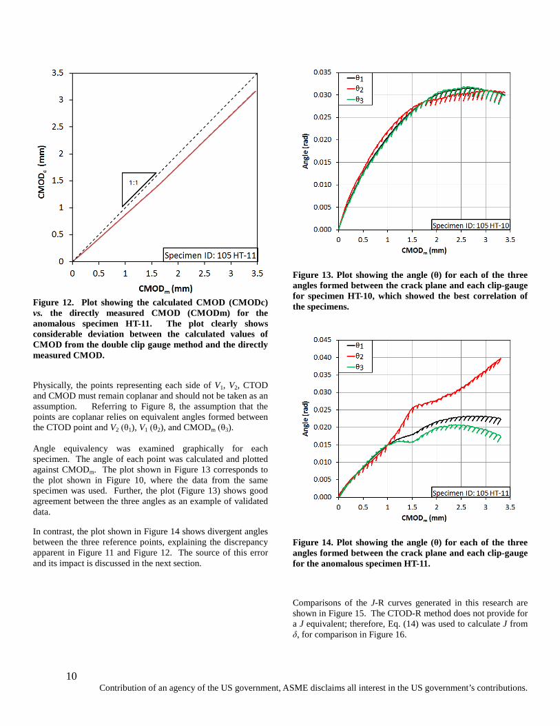
Figure 12. Plot showing the calculated CMOD (CMODc) vs. the directly measured CMOD (CMODm) for the anomalous specimen HT-11. The plot clearly shows considerable deviation between the calculated values of CMOD from the double clip gauge method and the directly measured CMOD.

Physically, the points representing each side of V1, V2, CTOD and CMOD must remain coplanar and should not be taken as an assumption. Referring to Figure 8, the assumption that the points are coplanar relies on equivalent angles formed between the CTOD point and V2 (θ1), V1 (θ2), and CMODm (θ3). Angle equivalency was examined graphically for each specimen. The angle of each point was calculated and plotted against CMODm. The plot shown in Figure 13 corresponds to the plot shown in Figure 10, where the data from the same specimen was used. Further, the plot (Figure 13) shows good agreement between the three angles as an example of validated data.

In contrast, the plot shown in Figure 14 shows divergent angles between the three reference points, explaining the discrepancy apparent in Figure 11 and Figure 12. The source of this error and its impact is discussed in the next section.

Figure 13. Plot showing the angle (θ) for each of the three angles formed between the crack plane and each clip-gauge for specimen HT-10, which showed the best correlation of the specimens.

Figure 14. Plot showing the angle (θ) for each of the three angles formed between the crack plane and each clip-gauge for the anomalous specimen HT-11.

Comparisons of the J-R curves generated in this research are shown in Figure 15. The CTOD-R method does not provide for a J equivalent; therefore, Eq. (14) was used to calculate J from δ, for comparison in Figure 16.

10 Contribution of an agency of the US government, ASME disclaims all interest in the US government’s contributions.

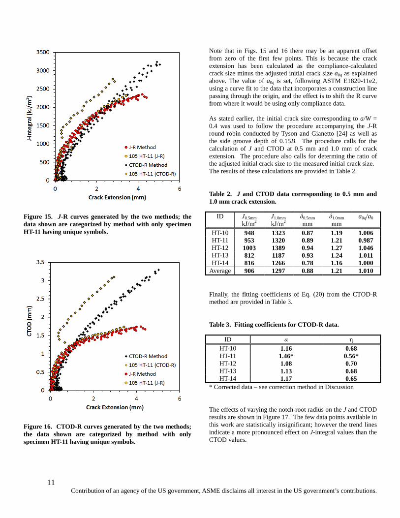
Figure 15. J-R curves generated by the two methods; the data shown are categorized by method with only specimen HT-11 having unique symbols.

Figure 16. CTOD-R curves generated by the two methods; the data shown are categorized by method with only specimen HT-11 having unique symbols.

Note that in Figs. 15 and 16 there may be an apparent offset from zero of the first few points. This is because the crack extension has been calculated as the compliance-calculated crack size minus the adjusted initial crack size a0q as explained above. The value of a0q is set, following ASTM E1820-11e2, using a curve fit to the data that incorporates a construction line passing through the origin, and the effect is to shift the R curve from where it would be using only compliance data. As stated earlier, the initial crack size corresponding to a/W = 0.4 was used to follow the procedure accompanying the J-R round robin conducted by Tyson and Gianetto [24] as well as the side groove depth of 0.15B. The procedure calls for the calculation of J and CTOD at 0.5 mm and 1.0 mm of crack extension. The procedure also calls for determing the ratio of the adjusted initial crack size to the measured initial crack size. The results of these calculations are provided in Table 2. Table 2. J and CTOD data corresponding to 0.5 mm and 1.0 mm crack extension.

ID J0.5mm kJ/m2

J1.0mm kJ/m2

δ0.5mm mm

δ1.0mm mm

a0q/a0

HT-10 948 1323 0.87 1.19 1.006 HT-11 953 1320 0.89 1.21 0.987 HT-12 1003 1389 0.94 1.27 1.046 HT-13 812 1187 0.93 1.24 1.011 HT-14 816 1266 0.78 1.16 1.000

Average 906 1297 0.88 1.21 1.010 Finally, the fitting coefficients of Eq. (20) from the CTOD-R method are provided in Table 3. Table 3. Fitting coefficients for CTOD-R data.

ID α η HT-10 1.16 0.68 HT-11 1.46* 0.56* HT-12 1.08 0.70 HT-13 1.13 0.68 HT-14 1.17 0.65

* Corrected data – see correction method in Discussion The effects of varying the notch-root radius on the J and CTOD results are shown in Figure 17. The few data points available in this work are statistically insignificant; however the trend lines indicate a more pronounced effect on J-integral values than the CTOD values.

11 Contribution of an agency of the US government, ASME disclaims all interest in the US government’s contributions.

Figure 17. J-Integral and CTOD values plotted against the initial notch-root radius.

DISCUSSION Every attempt was made to satisfy the requirements and recommendations of both the J-R and the CTOD-R recommended practices. Notable deviations from recommended practices included the extent of side grooving as well as the initial crack size (a0/W). The J-R method recommended symmetric side grooves of depth 0.15B, whereas the recommended side grooves from the CTOD-R procedure are symmetrically 0.1B. Also, the round-robin conducted by Tyson and Gianetto [24] used an a0/W value of 0.4. This value of a0/W was maintained in the present work in order to directly compare the present results to those obtained in the round-robin, although the range of values recommended by ExxonMobil is 0.25 ≤ a0/W ≤ 0.35. Both methods require that the test be conducted on a clamped specimen with a distance between grips of 10W. The loading profile used in this set of experiments did not exactly follow that prescribed by either recommended practice, yet the intent for each element was satisfied. A 3 s hold time (vs. 5 s recommended in the CTOD-R method) at each increment prior to unloading ensured that the initial unloading data were primarily elastic. The CMOD increment between unloadings in the plastic region was set to obtain a reasonable resolution of crack extension throughout the test. These experiments used a CMOD increment of 0.15 mm, which converts to 0.01W; the increment value matched the CTOD-R method, except that the CTOD-R method limits the increment as measured by the clip-gauge V1 as opposed to the CMOD measurement used here. The J-R method limits the increment

of load-line displacement to be less than 0.1b0, where b0 = W-a0. Use of the load-line displacement as an increment will have a dramatic increasing effect on the spacing between successive unloading cycles. The unloading increment in these tests was less than the limits prescribed by both recommended practices. The J-R method matches the consensus standard for SE(B) testing that describes a load drop of 25 % of the incremental maximum load. The CTOD-R method recommends a load drop equal to 20 % of the maximum load attained during the test, which is not explicitly known prior to testing. The load drop in this work was fixed at 20 kN, and therefore the percentage drop changed as the incremental maximum changed. It is important to note that the incremental maximum load after the ultimate load of the test was the load at which the CMOD increment of 0.15 mm was reached. In comparison, the 20 kN load drop used here was approximately 12.5 % of the maximum load reached in each test. The load drop level used herein was used successfully in other SE(T) testing efforts by the authors and is not likely to be a significant source of error in determining the crack size by the UC method, provided that only elastic unloading data are fit. Furthermore, the load drop level does not impact the ability of this research to successfully compare the two test methods on the same specimen. Alignment of the specimen in the grips requires considerable attention by the test operator. Axial load-line alignment of the specimen with the test frame, along with the assumption of crack plane perpendicularity, will ensure that the crack plane is loaded in tension and that shear forces are minimized. The alignment should be verified prior to testing and should be corrected rather than noted if there are discrepancies. The errors associated with alignment are expected to be low for homogenous base material. Testing a weld and associated heat affected zone (HAZ), on the other hand, may present considerable difficulty and potentially cause large errors. Instrumentation selection came directly from each of the recommended practices. A notable change to the clip-gauges was the addition of yttria-stabilized zirconia ceramic beams. Electrical isolation improved the PD measurements, and the modifications to the clip-gauges did not impact the ability to accurately measure the opening displacements. Clip-gauge beam contact with the inside face of the knife-edge structure will result in a reduction of the opening displacement; however, a discontinuity in the data is not expected, and therefore it would be difficult to determine during post-test analysis whether contact was made. Assuming that there are symmetrical angles between both beams in contact with the knife-edges, contact interference should not be a problem within the anticipated measurement range of the clip-gauges. Should the notched beams not make a symmetric angle, errors could be superimposed on the opening displacement data. The weight of the clip-gauge and wiring is enough to make these contact angles asymmetric if the instrumentation isn’t carefully installed and supported.

12 Contribution of an agency of the US government, ASME disclaims all interest in the US government’s contributions.

Securing the double-clip-gauge mounting fixture to the surface of the specimen must be done carefully to avoid measurement errors. The comparison between the two methods here assumes that the opening displacement locations are coplanar and therefore normal to both the front face of the specimen and each side of the specimen. To meet this requirement, the double-clip-gauge mounting fixture was secured to the specimen while being clamped to a precision parallel bar with shims that use the specimen’s integral knife-edges as a reference. According to the procedure provided by ExxonMobil [22], “The knife-edges shall be in parallel alignment to a tolerance of 1 °.” This angular requirement is difficult to measure accurately; it is easier and more accurate to measure a difference in the initial opening over the length of the double-clip-gauge mounting fixture. At a length of 27 mm (the length of the double-clip-gauge mounting fixture) a 1 ° tolerance amounts to a 0.47 mm difference in initial opening. Further analysis on the effect of this tolerance on the measurement comparisons is needed. Aligning and securing the double-clip-gauge mounting fixture by use of a precision parallel bar ensured a tolerance of less than 0.01 mm on each specimen measured with digital calipers. Achieving that tolerance was possible, without significant effort or expense. Ensuring that the tolerance was kept throughout the test was not possible; as is evident in the test of HT-11. However, special care was taken to securely mount the double-clip-gage fixture to each specimen in this research. Slight errors encountered were visible only by comparing the directly measured CMOD to the calculated values and then by the associated angle plots. Without these comparisons, we would have assumed, in tests performed with only the double-clip-gage method, that mounting integrity remained constant throughout the test. Unless a sufficiently large anomaly was evident to indicate invalid data, this incorrect assumption could lead to erroneous results and potentially high data scatter. Notwithstanding, only the CTOD-R method provides a series of checks to validate the results based on the measured and predicted crack sizes. Except for HT-11, the initial crack size estimates were within the validity requirements, noting that for HT-12 the CTOD-R method had the largest difference of 0.49 mm. The difference in estimated crack growth for that specimen was also the highest at 0.14ap. The correlation for HT-12 between CMODm and CMODc was better than for HT-11 so it didn’t warrant an example in this paper; however, upon examining the angle plot, it was clear that some out-of-plane movement was occurring, especially at large crack extensions. Two sources of out of plane movement are hypothesized; first, the remaining ligament was experiencing lateral bending due to a non-symmetric crack front, and second, the double-clip-gage mounting fixture(s) was moving relative to its initial position. The first source suggested indirectly by examining the post-test fractographs in Figure 9. In the case of HT-11 with the largest error, the crack front is nearly straight and symmetric and

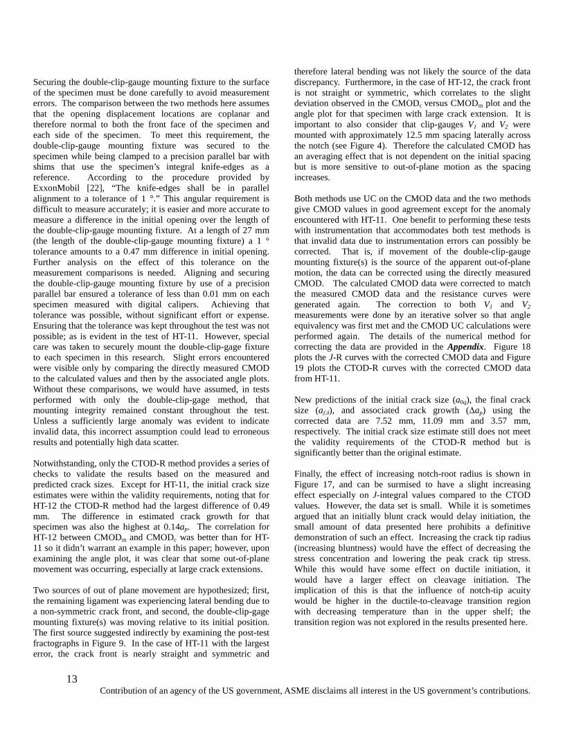
therefore lateral bending was not likely the source of the data discrepancy. Furthermore, in the case of HT-12, the crack front is not straight or symmetric, which correlates to the slight deviation observed in the CMODc versus CMODm plot and the angle plot for that specimen with large crack extension. It is important to also consider that clip-gauges V1 and V2 were mounted with approximately 12.5 mm spacing laterally across the notch (see Figure 4). Therefore the calculated CMOD has an averaging effect that is not dependent on the initial spacing but is more sensitive to out-of-plane motion as the spacing increases. Both methods use UC on the CMOD data and the two methods give CMOD values in good agreement except for the anomaly encountered with HT-11. One benefit to performing these tests with instrumentation that accommodates both test methods is that invalid data due to instrumentation errors can possibly be corrected. That is, if movement of the double-clip-gauge mounting fixture(s) is the source of the apparent out-of-plane motion, the data can be corrected using the directly measured CMOD. The calculated CMOD data were corrected to match the measured CMOD data and the resistance curves were generated again. The correction to both V1 and V2 measurements were done by an iterative solver so that angle equivalency was first met and the CMOD UC calculations were performed again. The details of the numerical method for correcting the data are provided in the Appendix. Figure 18 plots the J-R curves with the corrected CMOD data and Figure 19 plots the CTOD-R curves with the corrected CMOD data from HT-11. New predictions of the initial crack size (a0q), the final crack size (af,δ), and associated crack growth (Δap) using the corrected data are 7.52 mm, 11.09 mm and 3.57 mm, respectively. The initial crack size estimate still does not meet the validity requirements of the CTOD-R method but is significantly better than the original estimate. Finally, the effect of increasing notch-root radius is shown in Figure 17, and can be surmised to have a slight increasing effect especially on J-integral values compared to the CTOD values. However, the data set is small. While it is sometimes argued that an initially blunt crack would delay initiation, the small amount of data presented here prohibits a definitive demonstration of such an effect. Increasing the crack tip radius (increasing bluntness) would have the effect of decreasing the stress concentration and lowering the peak crack tip stress. While this would have some effect on ductile initiation, it would have a larger effect on cleavage initiation. The implication of this is that the influence of notch-tip acuity would be higher in the ductile-to-cleavage transition region with decreasing temperature than in the upper shelf; the transition region was not explored in the results presented here.

13 Contribution of an agency of the US government, ASME disclaims all interest in the US government’s contributions.

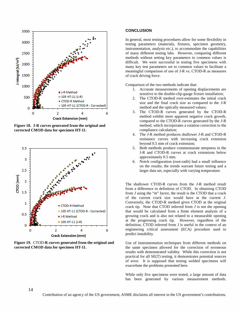
Figure 18. J-R curves generated from the original and corrected CMOD data for specimen HT-11.

Figure 19. CTOD-R curves generated from the original and corrected CMOD data for specimen HT-11.

CONCLUSION In general, most testing procedures allow for some flexibility in testing parameters (materials, fixtures, specimen geometry, instrumentation, analysis etc.), to accommodate the capabilities of many different testing labs. However, comparing different methods without setting key parameters to common values is difficult. We were successful in testing five specimens with many key test parameters set to common values to facilitate a meaningful comparison of use of J-R vs. CTOD-R as measures of crack driving force. Comparison of the two methods indicate that:

1. Accurate measurements of opening displacements are sensitive to the double-clip-gauge fixture installation;

2. The CTOD-R method over-estimates the initial crack size and the final crack size as compared to the J-R method and the optically measured values;

3. The CTOD-R curves generated by the CTOD-R method exhibit more apparent negative crack growth, compared to the CTOD-R curves generated by the J-R method, which incorporates a rotation correction to the compliance calculation;

4. The J-R method produces shallower J-R and CTOD-R resistance curves with increasing crack extension beyond 0.5 mm of crack extension;

5. Both methods produce commensurate steepness in the J-R and CTOD-R curves at crack extensions below approximately 0.5 mm.

6. Notch configuration (root-radii) had a small influence on the results; the trends warrant future testing and a larger data set, especially with varying temperature.

The shallower CTOD-R curves from the J-R method result from a difference in definition of CTOD. In obtaining CTOD from J using the “m” factor, the result is the CTOD that a crack of the current crack size would have at the current J. Conversely, the CTOD-R method gives CTOD at the original crack tip. Note that CTOD inferred from J is not the opening that would be calculated from a finite element analysis of a growing crack and is also not related to a measurable opening at the progressing crack tip. However, regardless of the definition, CTOD inferred from J is useful in the context of an engineering critical assessment (ECA) procedure used to predict instability. Use of instrumentation techniques from different methods on the same specimen allowed for the correction of erroneous results with demonstrated validity. While this correction is not practical for all SE(T) testing, it demonstrates potential sources of error. It is supposed that testing welded specimens will exacerbate the problems presented here. While only five specimens were tested, a large amount of data has been generated by various measurement methods.

14 Contribution of an agency of the US government, ASME disclaims all interest in the US government’s contributions.

Descriptions of the supplementary instrumentation (i.e., strain gages, extensometers and DCPD) and alternative data analysis techniques will be provided in a future publication. ACKNOWLEDGEMENTS Funding for this research was provided by the U.S. Department of Commerce, National Institute of Standards and Technology’s Pipeline and Infrastructure Safety Project. The authors are grateful to J.A. Gianetto and to W.R. Tyson of CanmetMATERIALS for providing test specimen blanks, guidance in conducting the tests according to the J-R round-robin procedure, and for valuable discussion regarding data analysis and interpretation. Finally, the authors are indebted to engineering technicians Ken Talley and Ross Rentz for their expert support in these experiments, and give special thanks to Robert Amaro for his assistance with data correction. REFERENCES 1. E1820-11e2, Standard Test Method for Measurment of

Fracture Toughness. 2011, ASTM International: West Conshohocken, PA, USA.

2. BS7448-1, Fracture Mechanics Toughness Tests - Part 1: Method for determination of KIc, Critical CTOD and Critical J Values of Metallic Materials. 1991, BSI.

3. ISO-12735, Metallic Materials - Determination of Plane-Strain Fracture Toughness. 2010, ISO.

4. Tang, H., Macia, M., Minnaar, K., Gioielli, P., Kibey, S., Fairchild, D. Developement of the SENT Test for Strain-Based Design of Welded Pipelines. in International Pipeline Conference. 2010. Calgary, Alberta, Canada: ASME.

5. Park, D.-Y., Tyson, W. R., Gianetto, J. A., Shen, G., Eagleson, R. S., Lucon, E. Weeks, T.S., Small-Scale Low-Constraint Fracture Toughness Test Results, in Final Report 277-T-06 to PHMSA, http://primis.phmsa.dot.gov/matrix/FilGet.rdm?fil=7330. Sept. 2011.

6. Park, D.-Y., Tyson, W. R., Gianetto, J. A., Shen, G., Eagleson, R. S., Lucon, E. Weeks, T.S., Small Scale Low Constraint Fracture Toughness Test Discussion and Analysis, in Final Report 277-T-07 to PHMSA, http://primis.phmsa.dot.gov/matrix/FilGet.rdm?fil=7331. Sept. 2011.

7. Cravero, S., Ruggieri, C., Estimation Procedure of J-Resistance Curves for SE(T) Fracture Specimens Using Unloading Compliance. Engineering Fracture Mechanics, 2007. 74(17): p. 2735-2757.

8. Park, D.Y., Tyson, W. R., Gianetto, J. A., Shen, G., Eagleson, R. S. Evaluation of Fracture Toughness of X100 Pipe Steel Using SE(B) and Clamped SE(T) Single Specimens. in International Pipeline Conference. 2010. Calgary, Alberta, Canada: ASME.

9. Pisarski, H.G., Wignal, C. M. Fracture Toughness Estimation for Pipeline Girth Welds. in International Pipeline Conference. 2002. Calgary, Alberta, Canada: ASME.

10. Pussegoda, L.N., Tiku, S., Tyson, W. R., Park, D. -Y., Gianetto, J. A., Shen, G., Pisarski, H. G. Comparison of Resistance Curves from Multi-Specimen and Single Specimen SEN(T) Tests. in International Offshore and Polar Engineering Conference. 2013. Anchorage, AK, USA: ISOPE.

11. Sarzosa, D.B., Ruggieri, C. Further Insights on J-R Curve Behavior in Pipeline Steels Using Low Constraint Fracture Specimens. in Pressure Vessels and Piping Conference. 2013. Paris, France: ASME.

12. Shen, G., Gianetto, J. A., Tyson, W. R., Development of Procedure for Low-Constraint Toughness Testing Using a Single-Specimen Technique, in MTL Report No. 2008-18 (TR). 2008, CanmetMATERIALS.

13. Shen, G., Tyson, W. R., Crack Size Evaluation Using Unloading Compliance in Single-Specimen Single-Edge Notched Tension Fracture Toughness Testing. Journal of Testing and Evaluation, 2009. 37(4).

14. Kalyanam, S., Wilkowski, GM, Shim, D-J, Brust, FW, Hioe, Y, Wall, G, Mincer, P. Why Conduct SEN (T) Tests and Considerations in Conducting/Analyzing SEN (T) Testing. in International Pipeline Conference. 2010. Calgary, Alberta, Canada: ASME.

15. Paredes, M. and C. Ruggieri. Effects of Weld Strength Mismatch on J and CTOD Estimation Procedures for SENT Fracture Specimens Based on Plastic Eta-Factors. in International Conference on Ocean, Offshore and Arctic Engineering. 2011. Rotterdam, The Netherlands: ASME.

16. Mathias, L.L., D.F. Sarzosa, and C. Ruggieri. Evaluation of Ductile Tearing of X-80 Pipeline Girth Welds Using SE (T), SE (B) and C (T) Fracture Specimens. in Pressure Vessels and Piping Conference. 2013. Paris, France: ASME.

17. Wang, E., Zhou, W., Shen, G. Duan, D. An Experimental Study on J (CTOD)-R Curves of Single Edge Tension Specimens for X80 Steel. in International Pipeline Conference. 2012. Calgary, Alberta, Canada: ASME.

18. Verstraete, M., Hertelé, S., Denys, R, Van Minnebruggen, K., De Waele, W., Evaluation and interpretation of ductile crack extension in SENT specimens using unloading compliance technique. Engineering Fracture Mechanics, 2014. 115: p. 190-203.

19. Hertelé, S., Verstraete, M., Denys, R., O’Dowd, N., J-integral analysis of heterogeneous mismatched girth welds in clamped single-edge notched tension specimens. International Journal of Pressure Vessels and Piping, 2014.

15 Contribution of an agency of the US government, ASME disclaims all interest in the US government’s contributions.

20. DNV-RP-F108, Recommended Practice: Fracture Control for Pipeline Installation Methods Introducing Cyclic Plastic Strain. 2006, Det Norske Veritas.

21. CanmetMATERIALS, Recommended Practice: Fracture Toughness Testing Using SE(T) Samples With Fixed-Grip Loading. 2010.

22. ExxonMobil, Measurement of Crack Tip Opening Displacement (CTOD) - Fracture Resistance Curves Using Single-Edge Notched Tension (SENT) Specimens. 2010.

23. Weeks, T.S., McColskey, J. D., Read, D. T., Richards, M. D. Fracture toughness instrumentation techniques for single-specimen clamped SE(T) tests on X100 line pipe steel: Experimental Setup. in Pipeline Technology Conference. 2013. Ostend, Belgium.

24. Tyson, W.R., Gianetto, J. A. Low-Constraint Toughness Testing: Results of a Round-robin on a Draft SE(T) Test Procedure. in Pressure Vessels and Piping Conference. 2013. Paris, France: ASME.

25. E399-12e1, Standard Test Method for Linear-Elastic Plane-Strain Fracture Toughness KIc of Metallic Materials. 2012, ASTM International: West Conshohocken, PA, USA.

26. Shen, G., J.A. Gianetto, and W.R. Tyson, Development of Procedure for Low-Constraint Toughness Testing Using a Single-Specimen Technique. 2008, MTL Report No. 2008-18 (TR) CanmetMATERIALS.

27. Joyce, J.A. and R.E. Link. Effect of Constraint on Upper Shelf Fracture Toughness. in Fracture Mechanics, 26th Volume. 1995. Philadelphia: ASTM.

28. Shen, G., Tyson, W. R. Evaluation of CTOD from J-integral for SE (T) specimens. in Pipeline Technology Conference. 2009. Ostend, Belgium.

APPENDIX This correction method should be applied only if the installation integrity of the double-clip-gage mounting fixture is compromised or suspect. If the clip-gauges measuring CMOD, V1, and V2 are coplanar then angle equivalency is maintained. The clip-gauge measuring CMOD is attached to integral knife edges on the surface of the specimen, and therefore will become the reference point by which all calculations are made. In the equations below, CMOD has been substituted by V0, and the following equations represent the geometry associated with the attachment points for each clip-gauge;

𝑆𝑆1 = sin𝜃𝜃1 =𝑉𝑉2 − 𝑉𝑉1

2(ℎ2 − ℎ1) , A(1)

𝑆𝑆2 = sin𝜃𝜃2 =𝑉𝑉1 − 𝑉𝑉0

2ℎ1 , A(2)

𝑆𝑆3 = sin𝜃𝜃3 =𝑉𝑉0 − 𝛿𝛿

2𝑎𝑎0 , A(3)

𝛿𝛿 = 𝑉𝑉1 −ℎ1 + 𝑎𝑎0ℎ2 − ℎ1

(𝑉𝑉2 − 𝑉𝑉1)

, and (by substitution) A(4)

𝑉𝑉0 =13

(4𝑉𝑉1 − 𝑉𝑉2) . A(5)

With the understanding that the angles (θ1, θ2 and θ3) should be equal, the following optimization function is used where a minimum value of the function represents an optimized condition. That is, when S1=S2=S3, the function goes to zero and therefore is perfectly optimized.

�(𝑆𝑆1 − 𝑆𝑆2)2 + (𝑆𝑆1 − 𝑆𝑆3)2 + (𝑆𝑆2 − 𝑆𝑆3)2 → 0 A(6) The method employed here is to make a guess for V1 and solve for V2. By inspection of Eq. A(2), it is clear that only V1 is unknown. Therefore the optimization routine solves Eq. A(2) for V1 and uses that relationship in Eqs. A(1), A(3) and A(4) where those relationships are used in Eq. A(6) to solve for V2. Once an optimized value for V2 is found, the value is used in Eq. A(5) to solve for V1. The process is repeated for each data collection time step corresponding to a new value of V0.

16 Contribution of an agency of the US government, ASME disclaims all interest in the US government’s contributions.