arX

iv:1

306.

2272

v1 [

cond

-mat

.mes

-hal

l] 1

0 Ju

n 20

13

Dirac Fermions in Solids — from High Tc cuprates and Graphene

to Topological Insulators and Weyl Semimetals.

Oskar Vafek

National High Magnetic Field Laboratory and Department of Physics,

Florida State University, Tallahassee, Florida 32306, USA

Ashvin Vishwanath

Department of Physics, University of California, Berkeley, California 94720, USA

Abstract

Understanding Dirac-like Fermions has become an imperative in modern condensed matter sci-

ences: all across its research frontier, from graphene to high Tc superconductors to the topological

insulators and beyond, various electronic systems exhibit properties which can be well described

by the Dirac equation. Such physics is no longer the exclusive domain of quantum field theories

and other esoteric mathematical musings; instead, real physics of real systems is governed by such

equations, and important materials science and practical implications hinge on our understanding

of Dirac particles in two and three dimensions. While the physics that gives rise to the massless

Dirac Fermions in each of the above mentioned materials is different, the low energy properties are

governed by the same Dirac kinematics. The aim of this article is to review a selected cross-section

of this vast field by highlighting the generalities, and contrasting the specifics, of several physical

systems.

1

CONTENTS

I. Dirac, Weyl, and Majorana 2

II. When and why to expect Dirac points in condensed matter? 4

A. Dirac points and Kramer’s pairs 6

B. Fermion doubling: Nielsen-Nynomiya theorem and ways around it 7

1. Domain wall Fermions and 3D topological insulators 8

III. Dirac particles subject to external perturbations 9

IV. Many-body interactions 16

V. Applications to various physical systems 20

A. Graphene 20

1. Coupling to external fields 22

B. Surface states of a 3D topological insulator 23

1. Coupling to external fields, interaction and disorder effects 25

C. dx2−y2-wave superconductivity in copper oxides 29

VI. Weyl Semimetals 33

A. Topological Properties 34

B. Physical Realizations 36

VII. Summary 37

VIII. Acknowledgments 38

References 38

I. DIRAC, WEYL, AND MAJORANA

I think it is a peculiarity of myself that I like to play about with equations,

just looking for beautiful mathematical relations which maybe don’t have any

physical meaning at all. Sometimes they do. - Paul A. M. Dirac (1902 - 1984)

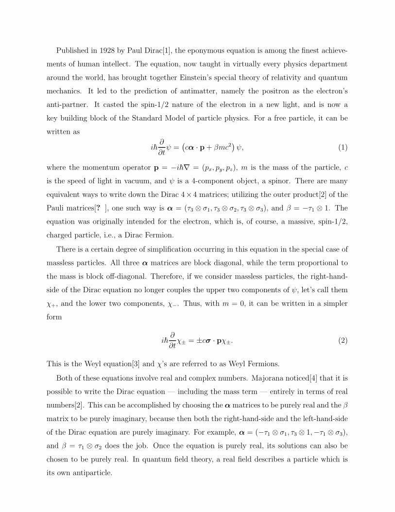
Published in 1928 by Paul Dirac[1], the eponymous equation is among the finest achieve-

ments of human intellect. The equation, now taught in virtually every physics department

around the world, has brought together Einstein’s special theory of relativity and quantum

mechanics. It led to the prediction of antimatter, namely the positron as the electron’s

anti-partner. It casted the spin-1/2 nature of the electron in a new light, and is now a

key building block of the Standard Model of particle physics. For a free particle, it can be

written as

i~∂

∂tψ =

(

cα · p+ βmc2)

ψ, (1)

where the momentum operator p = −i~∇ = (px, py, pz), m is the mass of the particle, c

is the speed of light in vacuum, and ψ is a 4-component object, a spinor. There are many

equivalent ways to write down the Dirac 4×4 matrices; utilizing the outer product[2] of the

Pauli matrices[? ], one such way is α = (τ3 ⊗ σ1, τ3 ⊗ σ2, τ3 ⊗ σ3), and β = −τ1 ⊗ 1. The

equation was originally intended for the electron, which is, of course, a massive, spin-1/2,

charged particle, i.e., a Dirac Fermion.

There is a certain degree of simplification occurring in this equation in the special case of

massless particles. All three α matrices are block diagonal, while the term proportional to

the mass is block off-diagonal. Therefore, if we consider massless particles, the right-hand-

side of the Dirac equation no longer couples the upper two components of ψ, let’s call them

χ+, and the lower two components, χ−. Thus, with m = 0, it can be written in a simpler

form

i~∂

∂tχ± = ±cσ · pχ±. (2)

This is the Weyl equation[3] and χ’s are referred to as Weyl Fermions.

Both of these equations involve real and complex numbers. Majorana noticed[4] that it is

possible to write the Dirac equation — including the mass term — entirely in terms of real

numbers[2]. This can be accomplished by choosing the αmatrices to be purely real and the β

matrix to be purely imaginary, because then both the right-hand-side and the left-hand-side

of the Dirac equation are purely imaginary. For example, α = (−τ1 ⊗ σ1, τ3 ⊗ 1,−τ1 ⊗ σ3),

and β = τ1 ⊗ σ2 does the job. Once the equation is purely real, its solutions can also be

chosen to be purely real. In quantum field theory, a real field describes a particle which is

its own antiparticle.

This review is about how such equations provide an accurate description of some 2- and

3-dimensional non-relativistic systems, where Dirac or Weyl Fermions emerge as low energy

excitations. It is also about how these excitations behave when subjected to external fields,

and how to relate the perturbing “potentials” (e.g. scalar, vector, mass etc.) appearing in

the effective Dirac equation to either externally applied fields produced in a laboratory, or

to defects and impurity potentials. A few consequences of many-body interactions will also

be reviewed. We will not discuss any of the fascinating aspects of Majorana Fermions in

condensed matter; this topic has already been covered in Ref.[5] and references therein. The

main topics of this paper form a vast area of physics, and we ask the reader to keep in mind

that it is impossible to do it justice in the review with a given allotted space.

II. WHEN AND WHY TO EXPECT DIRAC POINTS IN CONDENSED MAT-

TER?

In a non-relativistic condensed matter setting, the time evolution of any many body state

|Ψ〉 is governed by the Schrodinger equation

i~∂

∂t|Ψ〉 = H|Ψ〉 (3)

where H is the Hamiltonian operator. This Hamiltonian contains the kinetic energy of the

electrons and ions, as well as any interaction energy among them. Our aim is to illustrate

how and when we may expect the relativistic-like Dirac dispersion to arise from H in a cold

non-relativistic solid state. We do so first by pure symmetry considerations and then in a

brief survey of several physical systems realizing Dirac-like physics. We will assume that

the heavy ions have crystallized and to the first approximation let us ignore their motion.

As such, their role is solely to provide a static periodic potential which scatters the electron

Schrodinger waves and, if the spin-orbit coupling is also taken into account, the electron

spins. Then H → H0+Hint, where H0 includes all one body effects and Hint all many-body

electron-electron interaction effects.

According to the Bloch theorem, the energy spectrum En(k) and the eigenstates |φn,k〉 ofH0 can be described by a discrete band index n as well as a continuous D-dimensional vector

k, the crystalline momentum, which is defined within the first Brillouin zone. Consider now

two distinct but adjacent energy bands En+(k) and En−(k), and assume that for some range

of k the two bands approach each other, i.e. the energy difference |En+(k)−En−(k)| is much

smaller than the separation to any one of the rest of the energy bands. One way to derive the

effective Hamiltonian for the two bands is to start with a pair of (orthonormal) variational

Bloch states, |uk〉 and |vk〉, consistent with, and adapted to, the symmetries of H0. Then

the effective Hamiltonian takes the form

Heff =∑

k

ψ†kH(k)ψk (4)

where the first component of the creation operator ψ†k adds a particle (to the N -body state)

in the single particle state |uk〉 and antisymmetrizes the resulting N+1-body state. Similarly,

the second component creates a particle in the state |vk〉 and

H(k) =

〈uk|H0|uk〉 〈uk|H0|vk〉〈vk|H0|uk〉 〈vk|H0|vk〉

≡ f(k)12 +

3∑

j=1

gj(k)σj (5)

where 12 is a unit matrix and σj are the Pauli matrices. The corresponding one particle

spectrum is

E± = f(k)±

√

√

√

√

3∑

j=1

g2j (k). (6)

For a general k-point and in the absence of any other symmetries, gj(k) 6= 0 for each j. It

is clear from the expression for E±(k) that the two bands touch only if gj(k0) = 0 for each

j at some k0.

In 3D, we can vary each of the three components of k and try to find simultaneous zeros

of each of the three components of gj(k). To see that this may be possible without fine-

tuning, note that in general each one of the three equations gj(k) = 0 describes a 2D surface

in k-space. The first two surfaces may generally meet along lines, and such lines may then

intersect the third surface at points without additional fine-tuning. If such points exist,

they generally come in pairs and the dispersion near each may be linearized. The effective

Hamiltonian near one such point k0 takes the form

H(k) = Ek0+ ~v0 · (k− k0)12 +

3∑

j=1

~vj · (k− k0)σj . (7)

If v0 = 0 and the three velocity vectors vj are mutually orthogonal this has the form of

an anisotropic Weyl Hamiltonian. Of course, far away from k0 both bands may disperse

upwards or downwards, in which case even if the Fermi level could be set to E(k0), there

would be additional Fermi surface(s).

In 2D, only two components of k can be freely varied, and therefore it is impossible to find

simultaneous zeros of three functions gj(k) without additional fine-tuning. Simply stated,

in general, three curves do not intersect at the same point. Therefore, in the absence of

additional symmetries that may constrain the number of independent gj(k)’s, the two levels

will avoid each other.

A. Dirac points and Kramer’s pairs

We have intentionally refrained from any discussion of the electron spin degeneracy, or

time reversal symmetry, which were not assumed to be present in the above discussion. For

a number of physical systems considered later on, the product of the time reversal and the

space inversion leaves the crystalline Hamiltonian invariant. This symmetry implies that,

at each k, every electronic level is doubly degenerate, because if φk(r) is an eigenstate,

then so is its orthogonal Kramers partner, iσ2φ∗k(−r), where σ2 acts on the spin part of

the wavefunction. Therefore, the appropriate variational quadruplet of mutually orthogonal

states describing two nearby bands can be constructed from u1k(r)| ↑〉 + u2k(r)| ↓〉, its

Kramers partner −u∗1k(−r)| ↓〉 + u∗2k(−r)| ↑〉, and v1k(r)| ↑〉 + v2k(r)| ↓〉, with its partner

−v∗1k(−r)| ↓〉+ v∗2k(−r)| ↑〉. In this four-dimensional subspace

H(k) = f(k)14 +

5∑

j=1

gj(k)Γj (8)

where Γ1 = τ3 ⊗ 1, Γ2 = τ1 ⊗ 1, Γ3 = τ2 ⊗ σ3, Γ4 = τ2 ⊗ σ1, and Γ5 = τ2 ⊗ σ2; the first

Pauli matrix acts within the u,v space and the second within the Kramers doublets. While

the corresponding one particle spectrum, E± = f(k) ±√

∑5

j=1g2j (k), exhibits a two-fold

degeneracy at any k, an intersection of two Kramers pairs requires finding simultaneous zeros

of five gj(k)’s. Clearly, the bands avoid each other because, even in 3D, this condition cannot

be satisfied without additional symmetry. For example, if the spin-orbit interaction can be

neglected and time reversal symmetry is preserved — based on our earlier assumptions,

this also implies that space inversion is preserved — then the spin SU(2) symmetry forces

g3 = g4 = g5 = 0. With such additional symmetry, in 3D, the accidental degeneracy may

happen along 1D k-space curves and in 2D, at nodal points.

B. Fermion doubling: Nielsen-Nynomiya theorem and ways around it

The Nielsen-Nynomiya theorem states that it is impossible to construct a non-interacting

lattice hopping model with a net imbalance in the number of (massless) Dirac Fermions with

positive and negative chirality, provided that certain weak restrictions apply. For example,

the translationally invariant hopping amplitudes are assumed to decay sufficiently fast so

that in momentum space the Hamiltonian is continuous. The full proof[6] makes use of

homotopy theory and is beyond the scope of this review; pedagogical discussion of this “no-

go” theorem can be found in [7]. Here we will illustrate the basic idea behind it in a simple

example in two space dimensions.

Consider a model with two bands which may touch, such as the one given in Eq.(5) with

g3(k) = 0. Then, g1(k) and g2(k) are smooth periodic functions of kx and ky. If the first

function vanishes along some curve in the Brillouin zone, say the one marked by red in Fig.1,

and the second vanishes along another curve, blue in Fig.1, then the places where the two

curves intersect correspond to massless Dirac Fermions. Periodicity guarantees that any

intersection must occur at an even number of points, corresponding to an even number of

massless Fermions; just touching the two curves does not produce a Dirac Fermion because

at least one component of the velocity vanishes. Importantly, there is an equal number of

partners with opposite chirality.

One way to remove half of the massless Fermions is to bring back g3(k) and to force it

to vanish at only half of the intersections of the red and the blue curves in Fig.1. This

gaps out the unwanted Dirac points, leaving an odd number of gapless points. Haldane’s

model for a quantum Hall effect without Landau levels is a condensed matter example

where such an effect occurs along the phase boundaries separating quantum Hall phases and

trivial insulating phases[8]. HgTe quantum wells are another example[9]; there such “single

valley” massless Dirac Fermions have been experimentally realized at the phase boundary

separating the quantum spin Hall phase[10] and a trivial insulating phase. In the lattice

regularization of the relativistic high energy theory, for which the space-time points are

discrete and separated by at least a lattice constant a, a similar term corresponds to the

so-called Wilson mass term: a 4-momentum dependent mass,∑4

j=0∆(1− cos(kja))), which

vanishes at k = 0 and ω = 0. Adding the Wilson mass results in only one massless Fermion,

but it is not chiral. Moreover, in any condensed matter setting, making the k-dependent

P1

P2

+

-

+

-

+

+

-

-

kx

ky

FIG. 1: Illustration of the Fermion doubling in the 2D lattice hamiltonian. The blue and

red lines correspond to the solutions of g1(k) = 0 and g2(k) = 0, respectively. Both g1(k)

and g2(k) are smooth and must be periodic (for illustration only 4 Brillouin zones are

shown). Note that there is always an even number of intersections unless the two curves

just touch. If we think of the two signs as points in the complex plane, we see that the

gapless points have opposite chirality. Imagine displacing, say, the blue curve down,

holding the red curve fixed. The two points P1 and P2 will move towards each other, and

meet when the two curves touch. In this case, one of the Dirac velocities vanishes and we

do not have a Dirac Fermion at all. Therefore, in any lattice formulation with finite range

hopping, there will always be an even number of — in general anisotropic — massless

Dirac Fermions with opposite chirality.

mass term vanish at an isolated k-point requires fine tuning, and therefore such gapless

points generally correspond to phase boundaries as opposed to phases[8][10].

1. Domain wall Fermions and 3D topological insulators

Another way of avoiding the Fermion doubling on the lattice has been well known in high

energy theory[11][12]. Kaplan’s idea has been to start with massive Fermions and to make

a mass domain wall along the non-physical 4th spatial dimension, hereby labeled by w. By

mass domain wall we mean that for positive w the mass is m0, and for negative w it is −m0.

For the w = 0 lattice site the mass vanishes. To this domain wall mass term add a Wilson

mass term. There is then a range of values of m0 for which we have a single chiral 3+1D

massless Dirac, i.e. Weyl, particle on the domain wall. For m0 < 2∆ this can be understood

as the two sides having a mass inversion at only one k-point, namely at the origin. This

was proposed as a method to simulate — on a lattice — chiral Fermions in odd space-time

dimensions: from 4+1D to 3+1D or from 2+1D to 1+1D.

Unlike the Wilson mass, its condensed matter reincarnation is frequency independent, al-

though of course momentum dependent. Massless domain wall Fermions have been discussed

by Volkov and Pankratov at a 2D interface between (3D) SnTe and PbTe[13]. Such mass-

less Dirac Fermions are similar to those appearing at the surface of strong 3D topological

insulators, although there is a difference: in the former case the mass sign change occurs at

an even number of points in the Brillouin zone while in the latter at an odd number[14][15].

III. DIRAC PARTICLES SUBJECT TO EXTERNAL PERTURBATIONS

For relativistic Dirac Fermions described by 4-component spinors, external perturbations

take the form of space-time dependent 4 × 4 matrices, which we denote by V (r, t). In the

Hamiltonian formalism

H =

∫

d3rψ†(r)(

cα · p+mc2β + V (r, t))

ψ(r). (9)

There are 16 linearly independent 4 × 4 matrices which can be chosen for V (r, t). In a

relativistic context, their physical meaning is determined by their properties under Lorentz

transformations.

1. If the matrix structure of V (r, t) is the same as β, it clearly acts as a space-time varying

mass; because it is a scalar under the Lorentz transformation it is also sometimes

referred to as a scalar potential[16].

2. Any V (r, t) of the form −eα · A(r, t) acts as the spatial component of the electro-

magnetic vector potential; it enters via minimal coupling.

3. If V (r, t) = eΦ(r, t), then it corresponds to the time component of the electro-magnetic

potential, or electrical potential.

4. Of the 11 remaining matrices, 6 are Lorentz tensor fields, 4 are pseudo-vectors and 1

is pseudo-scalar[16].

Before proceeding, it is important to stress that the appropriate V — which describes

how Dirac Fermions in a given condensed matter system react to, say, an external physical

magnetic field — depends on the system itself. For example, it is not the same in graphene

and d-wave superconductors. This will be elaborated on in later sections.

As mentioned earlier, for massless Dirac Fermions the kinetic energy term, α · p, canbe chosen to be block diagonal. If the external perturbation V (r, t) does not couple the

two Dirac points, then such perturbation is also block diagonal. In 2D — where p is a 2-

component vector — within each 2×2 block such perturbation can be identified to be either a

mass, or a 3-component electro-magnetic potential, A = (Φ, Ax, Ay). A constant mass term

opens a gap in the spectrum; this gap may close at the boundaries or defects, but persists

in their absence. Simply put, for any energy −m < E < m, the equation E2 = c2p2 +m2

forces p to be imaginary and the corresponding states can at best be evanescent. A constant

electric potential, Φ, shifts the energy eigenvalues; the constant space components, Ax or

Ay, shift the momentum. The situation is similar in 3D, except the 2 × 2 matrix, which in

2D could be identified with the mass-like term, does not open a gap in 3D. Rather, it also

shifts the momentum, and therefore should be thought of as another space component of

the the vector potential.

Such simple intuitive arguments[17] show why Dirac particles can be confined by a spa-

tially varying mass, but not by a spatially varying electric potential. This observation is

behind the famous Klein “paradox”[18]. Instead of confining the massless Dirac particles,

such an electric potential causes a transfer of states towards the Dirac point, a situation

loosely analogous to an impurity electric potential creating midgap states in semiconduc-

tors.

A uniform electric field, E = −∇Φ, accelerates charged massless Dirac particles and leads

to non-equilibrium phenomena; it produces charge electron-positron pairs out of the filled

Dirac sea via the Schwinger mechanism[19]. For massless Dirac particles in 2D such rate has

been calculated to be ∼ (eE)3/2 [19][20] and, argued to lead to electrical current increasing

as E3/2 above a finite field scale below which it is E-linear[21][22][23].

The effect of a static 1D plane-wave electrical potential, Φ(x, y) = Φ0 cos(qx), on 2D

massless Dirac Fermions was considered in Ref. [24]. Based on our discussion, we intu-

F

x

0.5 1.0 1.5 2.0

E

Ñcq

à0

E

dΕ N HΕ L

FIG. 2: Integrated single particle density of states for a massless Dirac Fermion in 2D

subject to a static 1D periodic electric potential Φ0 cos (qx), blue dots, where Φ0 = ~cq;

solid line is for a free massless Dirac particle. Note the buildup of the spectral weight

which is recovered only near the cutoff energy, much larger than the scale shown.

itively expect that such potential locally shifts the Fermi energy away from the Dirac point

and introduces electron-positron “stripe puddles”. The energy spectrum has a particle-

hole symmetry: for every eigenstate ψE(x, y) with an energy E, there is an eigenstate

σ3ψE (x+ π/q, y) with an energy −E. For this result we assumed that the kinetic energy

term is c (pxσ1 + pyσ2). The full quantum mechanical solution of this problem, performed

numerically using a large number of plane-wave states, shows that, while the energy spec-

trum remains gapless, the spectral weight is indeed shifted towards the Dirac point. This is

shown in Figure 2, where we compare the integrated density of states, starting from E = 0,

in the presence and absence of the periodic potential. Clearly there is an excess number of

states at low energy. Interestingly, the “lost” states are recovered at energies comparable to

the cutoff, which is much larger than Φ0. Analogous buildup of low energy density of states

underpins the interpretation of the measured low temperature specific heat of type-II nodal

d-wave superconductors in an external magnetic field, discussed in a later section.

On the other hand, a uniform magnetic field directed perpendicular to the 2D plane,

B = ∂Ay/∂x−∂Ax/∂y, quantizes the electron orbits. The resulting spectrum consists of dis-

-1- 2- 3-2- 5 0 1 2 3 2 5EWc

FIG. 3: Single particle density of states (orange) for a 2D charged massless Dirac Fermion

subject to a uniform magnetic field, the Landau levels have been broadened for easier

visualization; green line is the density of states for the free Dirac particle. The (step-like)

integrated density of states shows that the spectral weight is redistributed over the energy

window given by(√

n + 1−√n)

Ωc where Ωc ≡√2~c/ℓB, where ℓB =

√

~c/eB is the

magnetic length.

crete Landau levels at energies En = sgn(n)√

|n|Ωc where n = 0,±1,±2, . . ., Ωc =√2~c/ℓB,

and the magnetic length ℓB =√

~c/eB; this result is easily obtained by elementary meth-

ods, see for instance [25]. Therefore, unlike for a Schrodinger electron, the energy difference

between the Landau levels of a massless 2D Dirac electron decreases with increasing en-

ergy. Each Landau level is N -fold degenerate, where N = Area/ (2πℓ2B); the degeneracy,

being proportional to the sample area, is macroscopically large. As shown in Figure 3,

the uniform magnetic field causes redistribution of spectral weight over the energy interval(√

n+ 1−√n)

Ωc; the number of states which are ‘moved’ to the Landau levels equals to

the total number of states which would be present between the Landau levels in the absence

of the external B-field.

The effects of a perpendicular magnetic field and an in-plane electric field have been

studied in the context of proving the absence of the relativistic correction to quantum Hall

effect in ordinary 2D electron gas[26]. The eigenfunctions and eigenvalues can be determined

m

0.5 1.0 1.5 2.0

E

Ñcq

à0

E

dΕ N HΕ L

FIG. 4: Massless Dirac Fermion in 2D subject to the 1D periodic mass,

m(x, y) = m0 cos(qx) with m0 = cq. Note the suppression of the spectral weight, which is

recovered only near the cutoff energy, again, much larger than the scale shown.

analytically, either directly[26], or, if B > E, by first Lorentz boosting the space-time

coordinates and the Dirac spinors into a frame in which the electric field effectively disappears

and only the Lorentz contracted magnetic field enters[27] [we discussed this simpler problem

above] and then ‘inverse’ Lorentz boosting the wavefunctions and eigenenergies.

Effects of non-uniform Dirac mass are quite fascinating, particularly when the mass pro-

file is topologically non-trivial and can lead to fractionalization of Fermion’s quantum num-

bers. We will illustrate the effect for 1D Dirac particles, first published in 1976 by Ro-

man Jackiw and Claudio Rebbi[28]. The kinetic energy and the mass term together give

HJR = cσ1p + σ3m(x), where m(x) is fixed to approach ±m0 as x → ±∞, vanishing once

somewhere in between. One such kink configuration is, for example, m(x) = m0 tanh (x/ξ).

The spectrum of HJR is particle-hole symmetric, because for any state ψE(x) with en-

ergy E, there is a state σ2ψE(x) with energy −E. As we argued earlier, any “midgap”

state with −m0 < E < m0 must be localized. Let us therefore seek states at E = 0;

they must satisfy i~cσ1ψ′0(x) = m(x)σ3ψ0(x). If we write ψ0(x) = σ1χ0(x) and sub-

stitute, then we find ~cχ′0(x) = m(x)σ2χ0(x). The solution now follows immediately:

χ0(x) = N exp[

1

~c

∫ x

0dx′m(x′)σ2

]

χ0(0). Since any χ0(0) can be decomposed into a lin-

ear combination of the +1 and −1 eigenvectors of σ2, we see that because the term in the

integral is positive, χ0 must be purely the −1 eigenvector,

1

−i

, otherwise the solution

is not normalizable. There is therefore a single isolated energy level at E = 0. For a general

single kink mass profile, there may be other mid-gap states, but they must come in pairs at

non-zero energies ±E.

The remarkable consequence of this isolation is that if the E = 0 midgap state is empty,

while all the negative energy states are occupied with charge e Fermions, then the resulting

state carries an excess localized charge of −e/2 relative to the ground state with uniform

mass without a kink. Similarly, if it is occupied, the excess charge is e/2. This follows from

the fact that a symmetric configuration of a widely separated kink and an anti-kink leads

to a pair of essentially zero energy states. In effect, one level has been “drawn” from the

“conduction band” and one from the “valence band”, each of which are missing one state.

If the zero energy doublet is unoccupied, then the total charge of this state differs from the

constant mass state by −e. Because the two localized states at the kink and the anti-kink

are perfectly symmetric, we must find that the total amount of charge in the vicinity of

each kink is the same, namely, −e/2 more than in the undistorted vacuum. If the vacuum

is neutral, then each kink carries half-integral charge. Since in any physical set up with

periodic boundary conditions every kink must have a corresponding anti-kink, the quantum

number fractionalization happens only locally. Globally, the charge changes by integral

units. Interestingly, if the particle-hole symmetry is weakly broken by adding to HJR a

small constant term proportional to σ2, then the localized states carry irrational charge[29].

Such ideas have fascinating applications to the physics of conducting polymers[30][31] and

there is an extensive literature on the subject reviewed in Ref.[32].

In higher dimensions, the topologically non-trivial configurations also lead to zero

modes[28][33]. Just as in 1D, such results are insensitive to the details of the mass configu-

ration, only the overall topology matters[34].

As an illustration of an effect a non-topological configuration of the mass has on a 2D

massless Dirac Fermion, we consider a 1D plane wave m(x, y) = m0 cos(qx). The resulting

Hamiltonian, c (pxσ1 + pyσ2) + m(x, y)σ3, has a particle hole symmetry, in that for every

eigenfunction ψE(x, y) with energy E, there is an eigenfunction σ3ψE(x+π/q, y) with energy

−E. The momentum along the y-axis, ky, is conserved due to the translational symmetry

in the y-direction. The momentum in the x-direction, kx, is conserved only modulo the

reciprocal lattice vector. At kx = ky = 0 we can construct the E = 0 state explicitly, just as

we did for the Jackiw-Rebbi problem, but now both choices for χ0 lead to Bloch normalizable

wavefunctions. There is therefore a doublet of states at k = 0 and E = 0. Away from k = 0,

there is a new anisotropic Dirac cone, with renormalized velocities. Interestingly, at k = 0,

the spectrum consists only of doublets at any energy because for every ψE(x, y) there is

σ2ψ∗E(x+ π/q, y) which is also at k = 0, has the same energy, and is orthogonal to ψE(x, y).

The overall effect on the integrated density of states is shown in Figure 4 for m0 = ~cq.

The minimum of the 2nd band is at E ≈ 1.1~cq and is responsible for the change of slope.

Overall, there is a suppression of the number of states at low energy — an opposite effect

compared to the electric potential case. Similarly, the “lost” states are recovered only at

energies comparable to the cutoff, which is much larger than m0.

To conclude this section, we briefly mention the chiral anomaly associated with the mass-

less Dirac equation[35][36]. The anomalies in quantum field theory are a rich subject[37] and

play a very important role in elementary particle physics[38]. In order to illustrate the effect,

note that the massless Dirac Hamiltonian in 3D and in the presence of an arbitrary external

electro-magnetic field,∫

d3rψ†(r)(

cα ·(

p− ecA(r, t)

)

+ eΦ(r, t))

ψ(r), formally commutes

with both the total particle number operator — or equivalently, the total charge operator —∫

d3rψ†(r)ψ(r), and the total “chiral” charge operator∫

d3rψ†(r)τ3 ⊗ 1ψ(r). Here we used

the representation for α used in Eq.(1). The equation of motion for an operator O(t) in the

Heisenberg picture is dO(t)/dt = [O(t), HH(t)] /i~, where HH(t) is the Dirac Hamiltonian in

the Heisenberg representation. Because the commutator vanishes for both the total charge

and the total “chiral” charge, they should both be constants of motion. However, closer

inspection reveals that in explicit calculations[35][36][38] an ultra-violet regularization must

be adopted in order to obtain finite results. What’s more, if the regularization is chosen in

such a way as to maintain the conservation of charge — a physically desirable consequence

of a useful theory — then for some configurations of electromagnetic fields, the chiral charge

is not conserved and changes in time. As an illustration, one such configuration consists of

a uniform magnetic field along the z-direction and a parallel weak electric field[38]. This

can be described by Φ = 0 and A(t) = (−By, 0, Az(t)) where the electric field is given by

−1

cddtAz(t); the time variation of Az(t) is therefore slow. For a system with size L3 and peri-

odic boundary conditions, the momentum is quantized in units of 2π/L and the separation

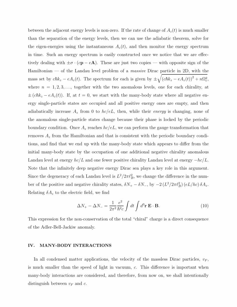
between the adjacent energy levels is non-zero. If the rate of change of Az(t) is much smaller

than the separation of the energy levels, then we can use the adiabatic theorem, solve for

the eigen-energies using the instantaneous Az(t), and then monitor the energy spectrum

in time. Such an energy spectrum is easily constructed once we notice that we are effec-

tively dealing with ±σ · (cp− eA). These are just two copies — with opposite sign of the

Hamiltonian — of the Landau level problem of a massive Dirac particle in 2D, with the

mass set by c~kz − eAz(t). The spectrum for each is given by ±√

(c~kz − eAz(t))2 + nΩ2

c ,

where n = 1, 2, 3, . . ., together with the two anomalous levels, one for each chirality, at

± (c~kz − eAz(t)). If, at t = 0, we start with the many-body state where all negative en-

ergy single-particle states are occupied and all positive energy ones are empty, and then

adiabatically increase Az from 0 to hc/eL, then, while their energy is changing, none of

the anomalous single-particle states change because their phase is locked by the periodic

boundary condition. Once Az reaches hc/eL, we can perform the gauge transformation that

removes Az from the Hamiltonian and that is consistent with the periodic boundary condi-

tions, and find that we end up with the many-body state which appears to differ from the

initial many-body state by the occupation of one additional negative chirality anomalous

Landau level at energy hc/L and one fewer positive chirality Landau level at energy −hc/L.Note that the infinitely deep negative energy Dirac sea plays a key role in this argument.

Since the degeneracy of each Landau level is L2/2πℓ2B, we change the difference in the num-

ber of the positive and negative chirality states, δN+ − δN−, by −2 (L2/2πℓ2B) (eL/hc) δAz.

Relating δAz to the electric field, we find

∆N+ −∆N− =1

2π2

e2

~2c

∫

dt

∫

d3r E ·B. (10)

This expression for the non-conservation of the total “chiral” charge is a direct consequence

of the Adler-Bell-Jackiw anomaly.

IV. MANY-BODY INTERACTIONS

In all condensed matter applications, the velocity of the massless Dirac particles, vF ,

is much smaller than the speed of light in vacuum, c. This difference is important when

many-body interactions are considered, and therefore, from now on, we shall intentionally

distinguish between vF and c.

In a 2D semi-metal such as graphene, we can imagine integrating out all high-energy

electronic modes outside of a finite energy interval about the Dirac point. The Fermi level is

assumed to be close to the energy of the Dirac point. Since none of the gapless modes have

been integrated out, there can be no non-analytic terms generated at long wavelengths,

and in particular no screening of the 1/r electron-electron interaction whose 2D Fourier

transform is, of course, non-analytic in momentum. Indeed, the long distance tail of the

bare electron-electron interactions falls off as e2/ (4πǫd r), where ǫd is the dielectric constant

of the 3D medium in which the graphene sheet has been embedded. At long distances,

ǫd is independent of the screening within the graphene sheet coming from the core carbon

electrons. This can be shown by solving an elementary electrostatic problem of a point

charge inserted in the middle of an infinite dielectric slab of finite thickness placed in a

3D medium with a dielectric constant ǫd [39][40][41]. At distances much greater than the

thickness of the slab, the Coulomb field within the slab is entirely determined by ǫd. A finite

on-site Hubbard-like interaction is usually taken to model the very short distance repulsion.

What then are the consequences of such electron-electron interactions if the Dirac point

coincides with the Fermi level? The importance of each of the terms can be determined

by dimensional analysis: in 2D, the Dirac field scales as an inverse length and therefore

the short distance (contact) coupling g, multiplying four Dirac fields, has dimensions of

length. In any perturbative series expansion, each power of g must be accompanied by a

power of an inverse length to maintain the correct dimensions of a physical quantity that

is being computed. Since it is critical, the only lengthscales in the problem are associated

with finite temperature, i.e. the thermal length ~vF/kBT , or the wavelength (frequency)

of the external perturbation. As such length scales become very long, each term in the

perturbative series in g becomes small and we expect the series to converge. In the parlance

of critical phenomena, the short range interaction is perturbatively irrelevant at the non-

interacting (Gaussian) fixed point (see e.g. Ref.[42]). Therefore, while there can be finite

modifications of the Fermi velocity or of the overlap of the true (dressed) quasiparticle with

the free electron wave function, the asymptotic infrared properties of the model must be

identical to the non-interacting Dirac problem[43, 44].

Using a similar analysis for the 1/r tail of the non-retarded Coulomb interaction, one

finds that e2/ (ǫd~vF ) is dimensionless. Despite the superficial similarity with the 3+1D

QED fine structure constant e2/~c, the physics here is different. First of all, the charge,

being a coefficient of a non-analytic term in the Hamiltonian, does not renormalize when

high energy modes are progressively integrated out[45][46]. Any renormalization group flow

of the dimensionless coupling e2/ (ǫd~vF ) must therefore originate in the flow of vF , which

is no longer fixed by the Lorentz invariance because such symmetry is violated by the

instantaneous Coulomb interaction. Detailed perturbative calculations reveal[47] that vF

grows to infinity logarithmically at long distances thereby shrinking e2/ (ǫd~vF ). Physically,

however, vF cannot exceed the speed of light c. Instead, once the retarded form of the

electron-electron interaction is properly included via an exchange of a (3D) photon, the flow

of vF saturates at c. The resulting theory is quite fascinating, in that the 2D massless Dirac

Fermions and the 3D photons propagate with the speed of light and, unlike in 3+1D QED,

the coupling e2/~c remains finite in the infra-red[47]. Unfortunately, since the flow of vF is

only logarithmic, and since initially there is a large disparity in the values of vF and c, such

a fixed point is practically unobservable. Instead, in practice, the physics is at best given

by the crossover regime in which vF increases, but never to values comparable to c.

The 1/r Coulomb interaction induced enhancement of the Fermi velocity is expected to

lead to a suppression of the low temperature specific heat below its non-interacting value

[48], as well as other thermodynamic quantities [49]. Interestingly, the suppression of the

single particle density of states does not lead to a suppression of the ac conductivity; in the

non-interacting limit it takes a (frequency independent) value σ0 = Ne2/16~ where N is the

number of the 2-component “flavors”. Again, the reason is the enhancement of the velocity:

loosely speaking, while there are fewer excitations at low energy, those that are left have a

higher velocity and therefore carry a larger electrical current. The expression [50] for the

low frequency ac conductivity has the form σ(ω) = σ0

(

1 + Ce2/(~vF + e2

4log vFΛ

ω))

, where

Λ is a large momentum cutoff. In the limit ω → 0, the correction to the non-interacting

value is seen to vanish[49][50][51]. The value of the (positive) constant C in this expression

has been a subject of debate as it seems to depend on the details of the UV regularization

procedure[50][51][52] [53][54][55]. Recently, the calculation of C within a honeycomb tight-

binding model [56], which provides a physical regularization of the short distance physics,

found C = 11/6 − π/2 ≈ 0.26; this value was also obtained within a continuum Dirac

formulation using dimensional regularization [53] by working in 2− ǫ space dimensions, and

eventually setting ǫ = 0.

Increasing the strength of the electron-electron interactions, while holding the kinetic

energy fixed, is expected to cause a quantum phase transition into an insulating state with a

spontaneously generated mass for the Dirac Fermions [57][58]. Since, as we just argued, weak

interactions are irrelevant at long distances, such transition must happen at strong coupling,

making it hard to control within a purely Fermionic theory. The full phase diagram also

depends on the details of the interaction and is difficult to determine reliably using analytical

methods. However, if one assumes that there is a direct continuous quantum phase transition

between the semi-metallic phase at weak coupling and a known broken-symmetry strong

coupling phase, say an anti-ferromagnetic insulator, then the critical theory can be argued

to take the form of massless Dirac Fermions Yukawa-like coupled to the self-interacting order

parameter bosonic field [59]. The advantage of this formulation is that the upper critical

(spatial) dimension is 3, and therefore such theory can be studied in 3− ǫ space dimensions

within a controlled ǫ-expansion, eventually extrapolating to 2 space dimensions by setting

ǫ = 1. The transition thus found is indeed continuous and governed by a fixed point at finite

Yukawa and quartic bosonic couplings. To leading order in ǫ, the critical exponents have

been determined[59]; for the semi-metal to the antiferromagnetic insulator quantum phase

transition, the correlation length exponent ν = 0.882 and the bosonic anomalous dimension

ηb = 0.8. Since the dynamical critical exponent has been found to be z = 1, these values

imply that the order parameter vanishes at the transition as |u − uc|β with the exponent

β = 0.794; here uc is a critical interaction. The 1/r Coulomb interaction has been found to

be irrelevant at this fixed point.

Given that at half-filling the theory does not suffer from the Fermion sign problem, a

very promising theoretical approach in this regard is numerical. The Hubbard model on

the honeycomb lattice, with the nearest neighbor hopping energy t and the repulsive on-

site interaction U , has been studied using quantum Monte Carlo methods [60][61][62][63].

Recent simulations on cluster sizes of up to 2592 sites show strong indications of a direct

continuous phase transition at U/t ≈ 3.869± 0.013 between the (Dirac) semi-metal and the

anti-ferromagnetic insulator[63], disfavouring earlier claims[62] on the existence of a spin

liquid phase for intermediate values of couplings 3.4 . U/t . 4.3 using smaller cluster sizes

of up to 648 sites. The critical exponent β = 0.8± 0.04 extracted in Ref.[63] is in excellent

agreement with the value obtained using the analytic Yukawa-like theory[59]. In subsequent

numerical simulations, the anti-ferromagnetic order parameter has been pinned by intro-

ducing a local symmetry breaking field[64]. The resulting induced local order parameter far

from the pinning center was then ‘measured’. This procedure resulted in an improved res-

olution, confirming a continuous quantum phase transition between the semi-metallic and

the insulating anti-ferromagnetic states. The single particle gap was found to track the

staggered magnetization, while the critical exponents obtained from finite size scaling agree

with those obtained to leading order in ǫ-expansion [59].

The 1/r Coulomb interaction can also be simulated efficiently without the Fermion

sign problem using a hybrid Monte Carlo algorithm [65] using either staggered Fermions

[65][66][67] or, preferentially, directly on a honeycomb tight-binding lattice[68][69][70][71][72].

The critical strength of the interaction necessary to achieve a quantum phase transition into

an insulating state seems to depend on the details of the short distance part of the re-

pulsion. Moreover, the system sizes studied numerically [72] may be too small to explore

the unscreened long distance tail of the 1/r interactions and to therefore unambiguously

establish theoretically whether suspended monolayer graphene should be insulating. It is

worth pointing out here that experiments on the suspended high purity monolayer graphene

samples show no sign of spontaneous symmetry breaking and would thus place it on the

semi-metallic side.

V. APPLICATIONS TO VARIOUS PHYSICAL SYSTEMS

A. Graphene

It is interesting to consider the massless Dirac Fermions in graphene[73] within the per-

spective outlined above. Pure symmetry arguments are a powerful tool in this regard; our

goal is to carry out such arguments in full detail in this section in order to illustrate their

utility. Assuming a perfectly flat, sp2 hybridized carbon sheet, the relevant atomic orbitals

forming both the conduction and the valence bands are the carbon 2pz orbitals[73][25]. A

good variational ansatz for u1k(r) would be∑

R eik·Rφpz(r − R − 1

2δ), where φpz(r) is a

Lowdin orbital[? ] with the same symmetry as the atomic pz orbital[74]. The exact form

of the Lowdin orbital is unimportant for us now, its symmetry is what matters. In an ide-

alized situation, without externally imposed strains or any other lattice distortions, the set

of vectors R could be chosen to span the triangular sublattice of the graphene honeycomb

lattice: mR1 + nR2 with R1 =√3x, R2 = 1

2R1 +

3

2ay, and m,n are integers. The basis

vector δ =√3

2ax + 1

2ay. Note that this Bloch state is manifestly periodic in k. Similarly,

we can choose v1k(r) as∑

R eik·Rφpz(r −R + 1

2δ). This physically motivated choice, along

with u2k(r) = v2k(r) = 0, defines our four basis states used to construct the Eq.(8).

A flat graphene sheet is invariant under the mirror reflection about the plane of the

lattice which further constrains H(k). Such operation reverses the in-plane components of

the electron spin — an axial vector — and leaves the perpendicular component unchanged,

thus acting on the spin state as a π-rotation about the axis perpendicular to the graphene

sheet. Additionally, the pz orbitals are odd under the mirror reflection. Therefore, the

effective Hamiltonian in Eq.8 is constrained to satisfy 1 ⊗ σ3 H(k) 1 ⊗ σ3 = H(k) for any

in-plane k. This forces g4 = g5 = 0 in the Eq.(8). Because the remaining three gj’s are in

general non-zero, we see that with only two components of k we cannot find simultaneous

zeros of three independent functions. Therefore, in the absence of any other symmetry, we

should expect level repulsion.

We can find the location of the Dirac points by taking into account additional symmetries.

The space inversion symmetry, say about the center of the honeycomb plaquette, requires

τ1⊗1 H(−k) τ1⊗1 = H(k). This forces g1(k) and g3(k) to be odd under k → −k and g2(k)

to be even. If the lattice also has a threefold symmetry axis perpendicular to the sheet and

passing through the plaquette center, then g2 and g3 must vanish at the two inequivalent

points k = ±K = ± 4π3√3ax, as well as, of course, all points equivalent to ±K by periodicity

in the momentum space. This follows from our formalism when we note that the effect of

the 2π3

rotation, induced on our wavefunctions by the operator e−i 2π3~

Lze−iπ3σ3 , affects our

four basis states as eiφτ3⊗σ3e−iπ31⊗σ3 , where φ = k′ · R1 and k′ is the result of rotating k

counter-clockwise by 120. Then, the identity eiφτ3⊗σ3H(k′)e−iφτ3⊗σ3 = H(k) evaluated at

k = ±K immediately leads to g2(±K) = g3(±K) = 0. Interestingly, g1 is finite at ±K with

vanishing derivatives, although if we also assumed spin SU(2) symmetry, which allows us to

flip the spins using τ1 ⊗ σ1, then g1 would vanish as well. In such case, irrespective of the

microscopic details of the full Hamiltonian, the two bands must touch at ±K.

The Dirac particles of graphene therefore live at ±K. Strictly speaking, they are not

quite massless because of non-zero spin-orbit coupling which makes g1(k) finite. Such a

term has been introduced by Kane and Mele[75]. However, this term is very small in planar

graphene structures, because the carbon atom is light and because graphene has a reflection

symmetry about the vertical plane passing through the nearest neighbor bond[76][77]. There

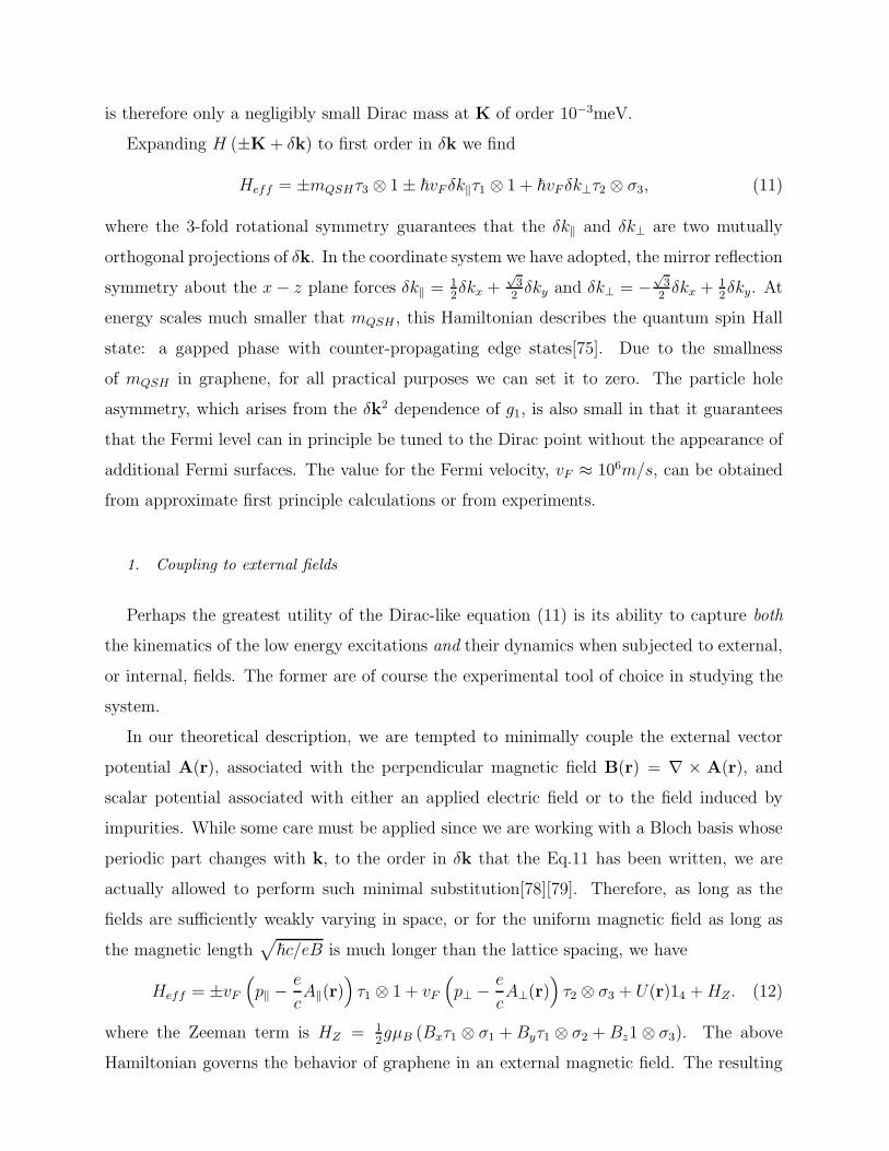
is therefore only a negligibly small Dirac mass at K of order 10−3meV.

Expanding H (±K + δk) to first order in δk we find

Heff = ±mQSHτ3 ⊗ 1± ~vF δk‖τ1 ⊗ 1 + ~vF δk⊥τ2 ⊗ σ3, (11)

where the 3-fold rotational symmetry guarantees that the δk‖ and δk⊥ are two mutually

orthogonal projections of δk. In the coordinate system we have adopted, the mirror reflection

symmetry about the x− z plane forces δk‖ =1

2δkx +

√3

2δky and δk⊥ = −

√3

2δkx +

1

2δky. At

energy scales much smaller that mQSH , this Hamiltonian describes the quantum spin Hall

state: a gapped phase with counter-propagating edge states[75]. Due to the smallness

of mQSH in graphene, for all practical purposes we can set it to zero. The particle hole

asymmetry, which arises from the δk2 dependence of g1, is also small in that it guarantees

that the Fermi level can in principle be tuned to the Dirac point without the appearance of

additional Fermi surfaces. The value for the Fermi velocity, vF ≈ 106m/s, can be obtained

from approximate first principle calculations or from experiments.

1. Coupling to external fields

Perhaps the greatest utility of the Dirac-like equation (11) is its ability to capture both

the kinematics of the low energy excitations and their dynamics when subjected to external,

or internal, fields. The former are of course the experimental tool of choice in studying the

system.

In our theoretical description, we are tempted to minimally couple the external vector

potential A(r), associated with the perpendicular magnetic field B(r) = ∇ × A(r), and

scalar potential associated with either an applied electric field or to the field induced by

impurities. While some care must be applied since we are working with a Bloch basis whose

periodic part changes with k, to the order in δk that the Eq.11 has been written, we are

actually allowed to perform such minimal substitution[78][79]. Therefore, as long as the

fields are sufficiently weakly varying in space, or for the uniform magnetic field as long as

the magnetic length√

~c/eB is much longer than the lattice spacing, we have

Heff = ±vF(

p‖ −e

cA‖(r)

)

τ1 ⊗ 1 + vF

(

p⊥ − e

cA⊥(r)

)

τ2 ⊗ σ3 + U(r)14 +HZ . (12)

where the Zeeman term is HZ = 1

2gµB (Bxτ1 ⊗ σ1 +Byτ1 ⊗ σ2 +Bz1⊗ σ3). The above

Hamiltonian governs the behavior of graphene in an external magnetic field. The resulting

Landau level structure has been directly observed in scanning tunneling spectroscopy[80][81][82].

Its utility in understanding the experiments on graphene hetero-junctions has been reviewed

in Ref.[18]. The Schwinger mechanism, discussed in Section III, has been experimentally

tested in Ref.[83]. Heff can also accommodate a time dependence of external poten-

tials, important for interpreting the optical[84] or infra-red spectroscopy measurements of

graphene[85]. The enhancement of the Fermi velocity, which, as discussed in Section IV, is

a signature of electron-electron interactions, have been reported in Ref.[86], with no signs of

gap opening at the Dirac point. The effects of strain, as an effective potential in Heff , are

discussed in Refs.[87][88][89]. By and large, realistic impurity potentials in graphene cannot

be treated in linear response theory[79][90]; the review of transport effects can be found in

Ref.[91].

B. Surface states of a 3D topological insulator

An example of a 3D topological insulator[14][15][92][93] is Bi2Se3[94][95][96]. Its excita-

tion spectrum is gapped in the 3D bulk, but its 2D surfaces accommodate gapless excitations

which carry electrical charge, conduct electricity, and the dispersion of the surface excita-

tions obeys massless Dirac equation. Unfortunately, presently the actual material suffers

from imperfections causing finite bulk conductivity, a complication which we will largely

overlook in this review.

The electronic configuration of Bi is 6s26p3 and of Se is 4s24p4. Since the p-shells

of Se lie ∼ 2.5eV below Bi[97], a naive valence count would suggest that the two Bi

atoms donate six of their valence p-electrons to fill the p-shell of Se. We would therefore

incorrectly conclude that the system is a simple, or trivial, insulator with a fully filled Se-

like p-band and empty Bi-like conduction band, perhaps with an appreciable band gap.

Interestingly, the strong spin-orbit coupling causes a “band inversion”[94][95] near the Γ-

point (the origin of the Brillouin zone), where the Bi-like states lie below the Se-like states.

Because the rhombohedral crystal structure of Bi2Se3 has a center of inversion, the exact

Bloch eigenstates must be either even or odd under space inversion at the crystal momenta

which map onto themselves under time reversal, modulo a reciprocal lattice vector, i.e.,

k = −k + G. Clearly, Γ is such a point. As shown by Fu and Kane [15], a sufficient

condition for a band insulator with a center of inversion to be a 3D topological insulator is

if such band inversion happens at an odd number of time reversal invariant points. More

precisely, the system is a 3D topological insulator if the product of the parity eigenvalues of

the occupied bands at the time reversal invariant k-points is odd, with the understanding

that we count the parity eigenvalue of only one of the members of the Kramers pair. This is

indeed what happens within a more realistic band structure calculation[94] [95] of Bi2Se3.

At the Γ point — but not at the other time reversal invariant k-points — the parity even

combination of the pz-like Bi states are spin-orbit coupled to the more energetic px± ipy-likeBi states, and get pushed below the parity odd combination of the Se pz-like and px±ipy-likestates.

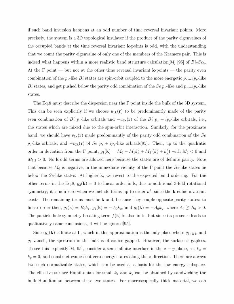
The Eq.8 must describe the dispersion near the Γ point inside the bulk of the 3D system.

This can be seen explicitly if we choose u1k(r) to be predominantly made of the parity

even combination of Bi pz-like orbitals and −u2k(r) of the Bi px + ipy-like orbitals; i.e.,

the states which are mixed due to the spin-orbit interaction. Similarly, for the proximate

band, we should have v1k(r) made predominantly of the parity odd combination of the Se

pz-like orbitals, and −v2k(r) of Se px + ipy-like orbitals[95]. Then, up to the quadratic

order in deviation from the Γ point, g1(k) = M0 +M1k2z +M2

(

k2x + k2y)

with M0 < 0 and

M1,2 > 0. No k-odd terms are allowed here because the states are of definite parity. Note

that because M0 is negative, in the immediate vicinity of the Γ point the Bi-like states lie

below the Se-like states. At higher k, we revert to the expected band ordering. For the

other terms in the Eq.8, g2(k) = 0 to linear order in k, due to additional 3-fold rotational

symmetry; it is non-zero when we include terms up to order k3, since the k-cubic invariant

exists. The remaining terms must be k odd, because they couple opposite parity states: to

linear order then, g3(k) = B0kz, g4(k) = −A0kx, and g5(k) = −A0ky, where A0 & B0 > 0.

The particle-hole symmetry breaking term f(k) is also finite, but since its presence leads to

qualitatively same conclusions, it will be ignored[95].

Since g1(k) is finite at Γ, which in this approximation is the only place where g3, g4, and

g5 vanish, the spectrum in the bulk is of course gapped. However, the surface is gapless.

To see this explicitly[94, 95], consider a semi-infinite interface in the x − y plane, set kx =

ky = 0, and construct evanescent zero energy states along the z-direction. There are always

two such normalizable states, which can be used as a basis for the low energy subspace.

The effective surface Hamiltonian for small kx and ky can be obtained by sandwiching the

bulk Hamiltonian between these two states. For macroscopically thick material, we can

ignore the exponentially small overlap between the surface states, and we find Hsurf =

±A0 (kxσy − kyσx), where the top sign is for the top surface, z = L, and the bottom sign for

the bottom surface z = −L. A similar procedure along the right, y = L, and left, y = −L,surfaces leads toHsurf = ± (B0kzσx + A0kxσz); the effective Hamiltonians are simply related

to each other by space inversion. In general,

Hsurf = n′ · (~σ × k′) (13)

where n′ is obtained by rotating the normal to the surface, n, by 180 about the z-axis,

and k′ = (−A0kx,−A0ky, B0kz). We thus arrive at an equation for massless, anisotropic,

Dirac particles. However, unlike in graphene which has four “flavors”, the surface of the 3D

topological insulator can support a single flavor.

1. Coupling to external fields, interaction and disorder effects

The existence of a single Dirac flavor on the surface of the 3D topological insulator has

important consequences for robustness of the surface states towards impurity disorder. The

states at k and at−k have opposite spin, leading to the suppression of back scattering[98][99]

and absence of localization for weak (scalar potential) disorder[100][101][102]. Theoretically,

such a (non-interacting) system is always expected to display electrical conductivity which

increases towards infinity as a logarithm of the system size. Recall that in graphene with

a pair of Dirac cones at K and −K, such back scattering is always present and therefore

weak localization is expected to eventually set in[103][104], although for smooth impurity

potentials, it may be very small[105][106].

Recent numerical study[107] of a topologically non-trivial 3D lattice model — with ran-

dom on-site energy intentionally placed only on the surface of the 3D system — indicates,

that the effective continuum description with Dirac particles scattered by a scalar potential

holds if the disorder strength is much weaker than the bulk gap (∼ 0.3eV in Bi2Se3). The

assertion is based on identification of Dirac-like features in a momentum resolved spectral

function, even when the translational symmetry of the lattice is broken by disorder. As the

typical disorder strength increases beyond the 3D bulk gap value, the surface states appear

diffusive. For even larger disorder strength, the outermost surface states are localized, but

weakly disordered Dirac-like states reappear directly beneath it. Apparently, for large sur-

face disorder, an interface between a strongly localized Anderson insulator and a topological

insulator is formed[107]. As such calculations were performed on finite size systems, which

are too small to detect an Anderson localization transition, it is presently impossible to

conclude whether there is a true phase transition at zero temperature separating the weak,

the moderate, and the strong disorder regimes. The combined effects of scalar disorder and

electron-electron (Coulomb) repulsion have been studied in Ref.[108] using the continuum

Dirac approximation. The authors argue that 3D topological insulators are different from

graphene, and that the single Dirac flavor makes the system metallic with finite conductivity

at zero temperature. Transport properties of topological insulators have been reviewed in

Ref.[109].

Because the electron spin is strongly coupled to its momentum, unlike in graphene, the

Zeeman coupling to the external magnetic field does not lead to simple spin splitting. Rather,

it opens up a gap, turning massless Dirac particles massive. To further illustrate the differ-

ence between the Dirac particles in a 3D topological insulator and graphene, consider now

the situation in which the external uniform magnetic field is applied along the z-axis, and

the field is sufficiently strong to quantize the orbital motion of the surface electrons. The

equation describing the states on the top and the bottom surfaces is then

[

±vF((

px +e

cBy

)

σy − pyσx

)

+ gzµBBσz

]

ψ(x, y,±L) = Eψ(x, y,±L), (14)

where ~vF = A0 and gz is the effective Lande g-factor. Indeed, the Zeeman coupling acts as

a Dirac mass and does not lead to the usual splitting of the spin degenerate energy levels.

It is straightforward to find the eigenvalues of this operator provided we are sufficiently far

from any edge. The resulting Landau level spectrum is

En = ±√

2A20

(

eB

~c

)

n+ (gzµBB)2, n = 1, 2, 3, . . . (15)

E0 = gzµBB. (16)

The physics in a quantizing magnetic field differs from graphene near the edge in another

important way: the top and the bottom surfaces are coupled through the side surfaces.

The applied magnetic field is parallel to the side surfaces and therefore there is no Landau

quantization along this surface; even the Zeeman term does not open up a gap on the side

surfaces, it merely shifts the momentum by a constant. Therefore, as the guiding center of

the Landau levels approaches the edge, they start mixing into the continuum of the states

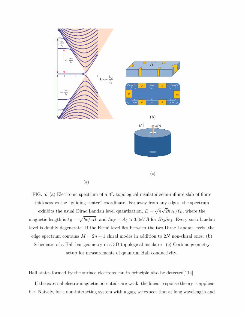
in the side surfaces. Fig.5 shows the electronic spectrum of a 3D topological insulator semi-

infinite slab of finite thickness vs. the “guiding center” coordinate. Far away from any

edges, the spectrum exhibits the usual Dirac Landau level quantization, E =√n√2~vF/ℓB,

where ℓB =√

~c/eB and forBi2Se3, vF = A0. Every such Landau level is doubly degenerate

because the top and the bottom surfaces are assumed to be identical. Such degeneracy would

be lifted if the inversion symmetry is broken by, say, a constant chemical potential difference

between the top and the bottom surfaces. As the guiding center coordinate approaches the

right edge — or the outer edge for the “Corbino” geometry — the Landau level states merge

with the plane-wave states from the vertical side surface. In the limit of very large thickness

such plane-wave states form a Dirac continuum.

This poses interesting questions: how robust is the quantum Hall effect and how to

measure it[110]? If the Fermi energy lies between the two Landau levels, the spectrum

contains M = 2n + 1 chiral edge modes in addition to 2N non-chiral ones. Clearly, in

any Hall bar geometry the leads necessarily couple to the continuum of the states in the

side surfaces, which present additional (unwanted) channels of conduction. Assuming that

the side modes equilibrate with each other and result in a finite conductivity, the chemical

potential will drop smoothly between µR and µL along each edge, and no quantization

of Hall conductance is expected[110][111][112]. Interestingly, quantization of σxy has been

reported in a strained 70-nm-thick HgTe layer[113], with a well developed plateau at ν = 2

and plateau-like features at ν = 3 and 4. At the same time, the longitudinal resistance

Rxx measured at 50mK shows a suppression by few tens of percents, but it does not reach

zero. While this observation awaits a complete theoretical treatment, if the sample is thin

then there are only a few non-chiral modes along the side surfaces which may get Anderson

localized with sufficient side surface roughness, leaving only chiral modes at the edges.

On the other hand, measurement of σxy in the Corbino geometry is expected to lead

to quantization[110][111]. The idea[111] is to perform the analog of the Laughlin thought

experiment, experimentally realized in 2D electron gas heterostructures in Ref.[114]. One

measures the amount of charge ∆Q transferred from the inner surface to the outer surface

in response to the induced EMF produced in the azimuthal direction by a slow change in the

magnetic flux ∆ϕ threading the sample. Then σxy = −c∆Q/∆ϕ. For σxy = n e2

h, half of the

charge travels through the top surface and the other half through the bottom surface. An

additional advantage of the Corbino setup is that any interaction-driven fractional quantum

2ÑvF

lB

6ÑvF

lB

2ÑvF

lB

klB -Ly

lB

-2 -1 1

H

N+M

N+M N+M

N+M

N N N

R

L

N+M

N N

N+M

N

(b)

H (t)

(c)

(a)

FIG. 5: (a) Electronic spectrum of a 3D topological insulator semi-infinite slab of finite

thickness vs the ”guiding center” coordinate. Far away from any edges, the spectrum

exhibits the usual Dirac Landau level quantization, E =√n√2~vF/ℓB, where the

magnetic length is ℓB =√

~c/eB, and ~vF = A0 ≈ 3.3eV A for Bi2Se3. Every such Landau

level is doubly degenerate. If the Fermi level lies between the two Dirac Landau levels, the

edge spectrum contains M = 2n+ 1 chiral modes in addition to 2N non-chiral ones. (b)

Schematic of a Hall bar geometry in a 3D topological insulator. (c) Corbino geometry

setup for measurements of quantum Hall conductivity.

Hall states formed by the surface electrons can in principle also be detected[114].

If the external electro-magnetic potentials are weak, the linear response theory is applica-

ble. Naively, for a non-interacting system with a gap, we expect that at long wavelength and

low frequency the response functions simply change, or renormalize, the dielectric constant

and the magnetic permeability; after all, the system is a dielectric insulator. Interestingly,

a 3D topological insulator gives rise to additional terms in the electro-magnetic response,

some of which are analogous to axion electrodynamics[115][116][117][118].

C. dx2−y2-wave superconductivity in copper oxides

Low energy quasiparticles obeying the Dirac equation may also emerge as a consequence

of a phase transition associated with the condensation of Cooper pairs. The specific example

which we consider here is the so called dx2−y2 pairing which occurs in cuprate high tempera-

ture superconductors [119][120]. In these layered, quasi 2D, materials, one may focus on the

electronic structure of a single CuO2 layer. A simple effective Hamiltonian for this system

is

H =∑

k,σ

(ǫk − µ) c†σ(k)cσ(k) +∑

k

(

∆kc†↑(k)c

†↓(−k) + h.c.

)

, (17)

where k = (kx, ky). The normal state dispersion, given by ǫk, describes a closed Fermi

surface, centered around (π, π), and equivalent points in momentum space. The anomalous

self-energy, ∆k, must in principle be determined from a microscopic theory; since such theory

is currently missing, one proceeds phenomenologically. Assuming time reversal symmetry,

ǫk = ǫ−k, and ∆k can be chosen real. Since it transforms as x2 − y2, it must change sign

under a 90 rotation and vanish along the Brillouin zone diagonals, where it intersects with

the Fermi surface at four inequivalent points. Weak orthorhombic distortions, such as in

YBCO, move the points of intersection slightly away from the zone diagonals[121], but do

not change the low energy physics in an important way.

The energy spectrum of the Fermionic quasiparticles can be obtained by solving the

Heisenberg equation of motion for c↑(k) and c†↓(−k):

i~∂

∂t

c↑(k)

c†↓(−k)

=

ǫk − µ ∆k

∆k −ǫk + µ

c↑(k)

c†↓(−k)

, (18)

finding E(k) =√

(ǫk − µ)2 +∆2k. Near the points of intersection between the Fermi surface

and the zeros of ∆k, we may expand ǫk −µ ≈ ~vFk⊥ and ∆k ≈ ~v∆k‖, where k⊥ and k‖ are

the deviation perpendicular and parallel to the Fermi surface respectively. In the vicinity of

such points, the above has the form of an anisotropic massless Dirac equation.

Interestingly, the Dirac node remains at zero energy even as the chemical potential, µ,

is varied. This is unlike in the previous examples, which involved Dirac particles in semi-

conductors, where µ must be fine tuned to coincide with the Dirac node, otherwise we have

Fermi circles with finite density of states at zero energy. Furthermore, given that the system

is a superconductor, the long range Coulomb interaction is screened. Since the discovery of

cuprates being dx2−y2 superconductors, there has been a tremendous effort in trying to un-

derstand the role of various perturbations. Here we focus on the question ‘How does such a

system behave in an external magnetic field?’[122][123][124][125][126] The first step towards

answering this question is to recognize that the upper and the lower components of the

‘spinor’ in Eq.18 acquire an opposite phase under a U(1) charge gauge transformation, and

therefore, an external magnetic field cannot couple minimally[126][127][128][129][130][131].

Moreover, the pair potential must also be modified. In a mean-field calculation, it is com-

puted self-consistently, with the solution depending on the value of the external magnetic

field[123][125]. But even in the absence of a microscopic theory — which may justify a

self-consistent mean-field calculation — we can establish this fact by noting, that near the

transition temperature, the existence of the Ginzburg-Landau functional follows quite gen-

erally from the order parameter having the charge 2e and the transition being continuous.

Given that in cuprates the magnetic penetration depth is much longer than the coherence

length, for most of the magnetic field range the field penetrates in the form flux tubes and

the order parameter phase winds by 2π near the core of each vortex. Therefore, in the

presence of the external magnetic field, the equation which generalizes Eq.18 is

i~∂

∂t

cr↑

c†r↓

=∑

r′

trr′ − µ↑δrr′ ∆rr′

∆∗rr′ −t∗rr′ + µ↓δrr′

cr′↑

c†r′↓

, (19)

where we assumed that the electrons hop on a square lattice given by r, with a complex

amplitude trr′. The phase of the complex singlet pair potential ∆rr′ winds by 2π when

its center of mass coordinate encircles a vortex sufficiently far from the vortex core; its

dependence on the relative coordinate has dx2−y2 symmetry.

When the typical separation between vortices, set by√

hc/eB, is much smaller than the

penetration depth, the magnetic field inside is almost uniform. Clearly, in such a case, the

plane waves with the wave-number k are no longer eigenstates of the kinetic energy operator.

One may attempt to proceed by working with Landau levels, which, in the continuum limit

of the above lattice model, are eigenstates of the kinetic energy operator for a uniform

magnetic field[125]. However, the number of the Landau levels below the Fermi energy,

as determined from the quantum oscillations experiments on the overdoped side of the

phase diagram[132][133], is of order 104 at magnetic fields of 1Tesla, this number decreasing

with 1/B. The energy scale associated with the pair potential is approximately given by

(v∆/vF )EF , decreasing the number of Landau levels mixed by ∆rr′ by only one order of

magnitude. Moreover, the resulting Hamiltonian matrix is dense, prohibiting the use of

efficient algorithms for determining the eigenvalues of sparse matrices.

In the relevant magnetic field range Hc1 ≪ H ≪ Hc2 a different approach was proposed

by Franz and Tesanovic[126], circumventing the use of the Landau level basis. The idea is

to map the problem onto an equivalent one but at zero average magnetic field, in which

case the plane wave basis may be used. This can be accomplished by performing a singular

gauge transformation, familiar in the context of the fractional quantum Hall effect. They

then argued that the relevant low energy excitations reside in the vicinity of the Dirac

nodal points, and that, in the continuum limit, the vortices together with the magnetic field

act as an effective potential scattering the Dirac particles. As the magnetic field decreases

so does the strength of the effective potential, making a natural connection with the zero

field problem. For each of the four massless Dirac particles, which were assumed to be

decoupled[124], the combination vF ·(

~

2∇φ− e

cA)

entered the Dirac equation as an effective

electrical potential, Φ [126]. Here∇×A = B and∇×∇φ = 2πz∑

j δ(r−Rj). The additional

minus signs acquired by the quasiparticles upon encircling an odd number of vortices was

encoded using a statistical U(1) field, minimally coupled to the Dirac particles[126]. Such

an approach provided an explicit method to (numerically) compute the scaling functions,

whose existence was proposed earlier by Simon and Lee[124], as well as to test the validity

of the semiclassical approach advanced by Volovik[122].

In the vicinity of each vortex, the effective potential ~

2∇φ− e

cA grows with the inverse of

the distance to the vortex. Since the kinetic energy of a massless Dirac particle also scales

with inverse length, the vortices constitute a singular potential. It is therefore not obvious

that the long wavelength expansion, which led to the effective Dirac description in the first

place, can be directly applied. Indeed, in the continuum limit, one must carefully specify

the boundary conditions at the vortex core by requiring that the effective Hamiltonian is

a self-adjoint operator[134]. A choice of such, so called, self-adjoint extensions should be

determined by matching to a well regularized lattice theory. Unfortunately, so far, it has

not been possible to determine their form. Since the choice is not unique, and since different

physically allowable choices appear to lead to a qualitative difference in the low energy

spectra (e.g. gapped or gapless), one is led to work with the lattice theory[128][130][135][136].

The usual choice is to set trr′ = −te−iArr

′ where the magnetic flux, ϕ, through an elementary

plaquette enters the Peierls factor via Arr+x = −πyeϕ/hc and Arr+y = πxeϕ/hc. The ansatz

for the pairing term is ∆rr+δ = ∆0ηδeiθ

rr+δ , where the dx2−y2-wave symmetry is encoded by

ηδ = +(−) for δ ‖ x(y), and the vortex phase factor eiθrr′ =(

eiφr + eiφr′

)

/|eiφr + eiφr′ |. This

choice is motivated by its behavior in the long distance limit[128][137].

For a periodic vortex arrangement, and after the appropriate lattice version of the singular

gauge transformation, one can take advantage of the Bloch theorem. The quasiparticle

spectrum is then a function of a “vortex crystal” momentum q. It can be shown[130] that

if the vortex lattice has a center of inversion and if the Zeeman term is ignored, then for

each eigenstate with an eigenvalue E at q, there is a corresponding eigenstate with an

eigenvalue −E at the same q. Therefore, any zero energy state at a fixed q must be at least

two-fold degenerate. However, because our problem breaks time reversal symmetry, such

a degeneracy can only be achieved by fine tuning an additional parameter besides the two

components of q. Therefore, the quasiparticle spectrum of an inversion symmetric vortex

lattice is in general gapped. The Zeeman term corresponds to a simple overall shift of the

quasiparticle energy and does not destroy the avoided crossing, it simply moves it to a non-

zero energy. Some further non-perturbative aspects of this problem have been discussed in

Ref.[135].

In Figure 6 we show the quasiparticle contribution to the specific heat obtained by the

numerical diagonalization of the resulting (sparse) Hamiltonian matrix for different values of

magnetic field. The result is re-scaled according to the Simon and Lee scaling[124][137]. We

see that in the mixed state of a dx2−y2 superconductor, for vF/v∆ = 7 and 14, increasing the

magnetic field indeed increases the specific heat in an intermediate temperature window,

in accord with the semiclassical prediction by Volovik[122]. At the lowest temperatures,

however, there is a crossover into the quantum regime where the interference effects set in

and the finite spectral gap rapidly decreases the specific heat. Note that the entropy at low

T , i.e.∫ T

0C(T ′)/T ′dT ′, increases with an increasing magnetic field. Entropy must of course

be conserved and independent of the magnetic field when T → ∞; the effect comes from the

transfer of the spectral weight from energies above ∼ ∆0. It is similar to the effect discussed

in the context of the Dirac particle in a periodic electrical potential whose average vanished,

see Fig.2.

We see then, that despite being described by similar kinematics, there is a very important

difference in the way the dx2−y2-wave Dirac particles couple to the physical external magnetic

field from the way the graphene or the 3D topological quasiparticles couple. In the latter

case, the specific heat may oscillate with the field, but when averaged over few oscillations,

its value is field independent. In the former case, it is the average value that increases with

the external field.

VI. WEYL SEMIMETALS

My work always tried to unite the truth with the beautiful, but when I

had to choose one or the other, I usually chose the beautiful. - Hermann Weyl

(1885-1955)

It has long been known that band touchings in three dimensions are very stable[144, 145], as

described in Section 2. When the chemical potential lines up with the band touching points,

and no other Fermi surfaces intersect it, a semimetal results. The low energy dispersion of

electrons then closely resembles the Weyl equation of particle physics, hence these semimetals

have been termed Weyl semimetals[146]. The generic form is shown in Equation 4. Initially,

the Weyl equation was believed to describe neutrinos, which however had to be given up with

with the discovery of neutrino mass. Thus, an experimental realization of a Weyl semimetal

would be the first physical realization of this fundamental equation. Here we will briefly

review topological aspects of Weyl semimetals and their possible realizations in solids. For

simplicity, consider the following simplified form of Equation 4:

H± = ±vF (pxσ1 + pyσ2 + pzσ3) (20)

where we have expanded about a pair of band touchings located at k± and have denoted

p = ~(k − k+) (for example). The Pauli matrices σj act in the space of the pair of bands

that approach each other and touch at the Weyl nodes. The energy spectrum then is

E(p) = vF |p| for both nodes. At each node we can associate a chirality, which measures

the relative handedness of the three momenta and the Pauli matrices associated in the Weyl

equation. The chirality is ±1 for the Hamiltonians H±. This is a general property of Weyl

Fermions realized in band structures - their net chirality must cancel. A simple physical proof

of this Fermion doubling theorem is pointed out below. In a clean system, where crystal

momentum is well defined, one can focus at one or the other node and hence effectively

realize the Weyl equation. Note, we have assumed that the bands are individually non-

degenerate. This requires that either the time reversal symmetry, or the inversion symmetry

(parity), is broken. In order to realize the minimal case of just a pair of opposite chirality

Weyl nodes, time reversal symmetry must be broken[146]. In practice this is achieved by

magnetic order in the crystal. Alternately, one may consider systems with broken inversion

symmetry[147], where a minimum of four Weyl nodes are present.

It is useful to describe a toy lattice model where the above dispersion is simply realized[148,

149]. Consider electrons hopping on a cubic lattice, where on every site the electron can be

spin up or down. Now, assume a spin-orbit type hopping in the y and z directions which

proceeds by flipping spin, while along the x direction the sign of hopping depends on the

spin projection. The coresponding Hamiltonian is

H(k) =~vFa

([cos(kxa) +m (2− cos(kya)− cos(kza))]σ1 + sin(kya)σ2 + sin(kza)σ3) . (21)

This Hamiltonian has Weyl nodes located at (±π/2a, 0, 0). Linearizing about these points

yields the Weyl equation 20. Note, one can add an arbitrary (Hermitian) term to this Hamil-

tonian, which will cause the nodes to shift but cannot remove them for small perturbations.

For example, a Zeeman field ∆H = − (~vF/a)hZσ1 shifts the nodes to (k±, 0, 0) where

k±a = ± cos−1 hZ . Essentially, this stability to perturbations arises from the fact that there

is no ‘fourth’ Pauli matrix available to gap out the node. Only when the field hZ is large

enough |hZ| ≥ 1 to move the Weyl point up against each other do they annihilate, leading

to a fully gapped insulator.

A. Topological Properties

The stability of the Weyl nodes is tied to a topological protection inherent to this band

structure. Away from the band touching points, there is a clear demarcation between filled

and empty bands. Consider the state obtained at a particular crystal momentum by filling

the negative energy states (below the chemical potential). By studying how this state evolves

on varying the crystal momenta one can extract a Berry phase, from which a Berry flux

B(k) = ∇k ×A(k) can be defined. The Weyl nodes are sources, or monopoles, of Berry flux

- thus ∇·B(k) = ±δ3(k−k±), hence their stability. They can only disappear by annihilating

a monopole of the opposite charge - which is a Weyl node of opposite chirality[150].

This band topology of Weyl semimetals has two direct physical consequences. The first

is an unusual type of surface state, unique to Weyl semimetals - called Fermi arcs [146].

Consider a 3D slab of Weyl semimetal with a surface in the x-y plane. Translation invariance

along these directions allow us to label single electron states by crystal momenta in this plane.

Let us assume we have a single pair of Weyl nodes in the bulk as in the model in Eq. 21.

At this same energy we can ask what are the surface states in the system. Surface states

are well defined at this energy at all momenta away from the Weyl nodes, because there

are no bulk excitations with the same energy and momenta. It is easily seen that surface

states should form a Fermi arc. The arc terminates at the crystal momenta corresponding

to the bulk Weyl nodes (see Figure 7). This result follows from the fact that Weyl nodes

are monopoles of Berry flux. Therefore, the 2D Brillouin zones that lie between the pair

of Weyl nodes will have a different Chern number than the planes outside (see Figure 7).

These planes may be interpreted as 2D Quantum Hall states associated with a chiral edge

state which is guaranteed to cross the chemical potential. The locus of these crossings gives

the Fermi Arc surface state.

If one considers both top and bottom surfaces of a Weyl semimetal one should recover a

closed Fermi surface as one would expect for a 2D system. Indeed the two Fermi arc states

on opposite surfaces, taken together, form a closed 2D Fermi surface. Thus a thin slab of

semimetal may be viewed as a 2D system with a closed Fermi surface. As the thickness is

increased, two halves of this Fermi surface are spatially separated to opposite sides of the

sample. Probing these surface states in surface sensitive probes such as ARPES and STM

should provide smoking gun evidence for this unusual phase of matter.

A second physical consequence of the topology of Weyl nodes is their response to an

applied electric and magnetic field. As discussed in Section III, a single Weyl node possesses

a Chiral Anomaly: the net number of charged particles would not be conserved if a single

Weyl node was present[36][35]. Rather the continuity equation is modified

∂n

∂t+∇ · J = ± 1

4π2

e2

~2cE ·B,

where the sign is determined by the chirality of the Weyl node. Thus charge conservation

provides a rationale for why Weyl nodes always must occur in a band structure with zero

net chirality. Although the net charge is then conserved, the chiral anomaly does lead to an

interesting effect. Consider for example the case of a pair of nodes with opposite chirality

as in Equation 21. Then the difference in density between excitations near the two nodes

(the valley polarization) is governed by

d(n+ − n−)

dt=

1

2π2

e2

~2cE ·B (22)

thus, applying parallel electric and magnetic fields can be used to control the valley polariza-

tion - which will lead to new transport phenomena and possibly even applications for Weyl

semimetals. There are close connections between this phenomena and the chiral hydrody-

namics recently described in the high energy literature[151]. A related physical effect is a

giant anomalous Hall effect expected for the case of a pair of Weyl nodes which is proportional

to the separation between the Weyl nodes in momentum space. Thus σyz = e2

2πh(k+ − k−).

If combined with an independent measurement of the momentum separation (k+ − k−) be-

tween Weyl nodes, obtained for example via ARPES, leads to a quantized ratio. In Weyl

semimetals with higher symmetry, such as cubic symmetry, the anomalous Hall conductance

vanishes. However, under a uniaxial strain that lowers symmetry, a large anomalous Hall

effect is expected[148].

We note that the two topological properties mentioned above required that the Weyl

nodes be separated in crystal momentum. In the presence of breaking of crystalline transla-

tion symmetry, such a distinction may be lost, which would obstruct defining a sharp physical

property that reflects the underlying topology. Thus it appears that while semimetals like

the Weyl semimetal may be topological states, the topology associated with them is sharply

defined in the presence of translation symmetry, in contrast to insulating topological phases

which do not require any such assumption. However, in practice disorder is rarely strong

enough to completely destroy well separated nodal points, as evidenced in the example of

graphene. Thus realistic systems should display the novel features we mentioned above.

B. Physical Realizations

Despite being a very natural band structure, currently there are no clearly established ma-

terials with Weyl nodes near the chemical potential, although several promising candidates

exist. It has been proposed that members of the family of material A2Ir2O7 (pyrochlore

iridates), where A = Y or a rare earth such as A = Eu, Nd, Sm may be in or proximate

to the Weyl semimetal phase[146]. This is currently an active area of experimental work

[152][153][154][155]. Spinels based on osmium[156] and HgCr2Se4[157] have also been pro-

posed as candidates. Another route has been to try to engineer Weyl semimetals using

heterostructures of topological insulators[158, 159]. Interestingly, a proposal to realize Weyl

points in a photonics band structure has recently appeared[160]. A general symmetry anal-

ysis of crystal structures that may host Weyl semimetals appeared in [161]. Further details

on this topic may be found in the longer review [162].

VII. SUMMARY

We reviewed general conditions under which one may expect gapless Dirac points to occur

in solids. Their appearance may be a consequence of band-structure effects, of symmetry

breaking due to many-body effects such as superconductivity or as a surface state of a bulk

topological phase. If a Dirac point exists, additional fine-tuning of the chemical potential

is necessary in order for the Dirac point to coincide with the Fermi level, unless the Dirac

point appears as a consequence of the condensation of Cooper pairs. Then, the Dirac point

“rides” along with the chemical potential.

We also reviewed how the Dirac Fermions respond to externally applied perturbations and

why the response differs in the case of graphene, topological insulators, Weyl semimetals,

and d-wave superconductors. External potentials cause a redistribution of the quasiparticle

spectral weight: space-dependent electrical potential tends to transfer the spectral weight

from large energies towards the Dirac point, while the Dirac mass term tends to remove

the states from the vicinity of the Dirac point, pushing them towards the large energies.

Uniform magnetic field redistributes the states over the energy scale set by the cyclotron

frequency. In this context, the magnetic field induced enhancement of the low temperature

specific heat in the vortex state of d-wave superconductors is also reviewed.

When weak, finite range electron-electron interactions result in only finite renormalization

of the Dirac particle dispersion, without leading to any qualitative changes. As the strength

of the interactions increases, a quantum phase transition occurs into an insulating state. In

the case of the half-filled repulsive Hubbard model on the honeycomb lattice, the transition

appears to be into a Neel anti-ferromagnetic state. Among its attractive features is the

possibility to study the transition either using a quantum Monte Carlo method without the

Fermion sign problem, or analytically using the ǫ-expansion around 3+1 dimensions for the

continuum field theory description with the massless Dirac particles Yukawa coupled to a

self-interacting O(3) bosonic field. Understanding why an interacting system may undergo

a symmetry breaking transition into a state with massless Dirac Fermions, such as in the

cuprate superconductors, rather than avail of a fully gapped state, remains a fascinating

open problem.

Finally we discussed recent developments of three dimensional Weyl Fermions, including

their robust topological properties in the form of unusual surface states and magneto-electric

responses, and possible physical realizations.

VIII. ACKNOWLEDGMENTS

OV was supported by the NSF CAREER award under Grant No. DMR-0955561, NSF

Cooperative Agreement No. DMR-0654118, and the State of Florida. AV was supported by

ARO MURI grant W911NF-12-0461.

[1] Dirac PAM. 1928 Proc. R. Soc. Lond. A 117(778):610-624

[2] Wilczek F. 2009. Nature Physics 5:614-618

[3] Weyl H. 1929. Zeitschrift fur Physik 56:330-352

[4] Majorana E. 1937. Nuovo Cimento 14:171-184

[5] Beenakker CWJ. 2013. Annual Reviews of Condensed Matter Physics 4:113136

[6] Nielsen HB, Ninomiya, M. 1981. Nuclear Physics B 185:2040

[7] Itzykson C, Drouffe J-M. 1989. Statistical Field Theory, Vol. 1., pp. 396. Cambridge, UK:

Cambridge University Press. 403 pp.

[8] Haldane FDM. 1988. Physical Review Letters 61:2015-2018

[9] Buttner B et.al. 2011. Nature Physics 7:418422

[10] Maciejko J, Hughes TL, Zhang S-C. 2011. Annual Reviews of Condensed Matter Physics

2:3153

[11] Kaplan DB. 1992. Physics Letters B 288:342-347

[12] Kaplan DB, Sun S. 2012. Physical Review Letters 108:181807(4)

[13] Volkov BA, Pankratov OA. 1985. JETP Letters 42:178-181

[14] Fu L, Kane CL, Mele EJ. 2007. Physical Review Letters 98:106803(4)

[15] Fu L, Kane CL. 2007. Physical Review B 76:045302(17)

[16] Thaller B. 1992. The Dirac Equation Springer-Verlag, Berlin, Heidelberg, New York .

[17] Ludwig AWW, Fisher MPA, Shankar R, Grinstein G. 1994. Physical Review B 50:7526-7552

[18] Young AF, Kim P. 2011. Annual Reviews of Condensed Matter Physics 2:101120

[19] Schwinger J. 1951. Physical Review 82:664-679

[20] Allor D, Cohen TD, McGady DA. 2008. Physical Review D 78:096009(5)

[21] Dora B, Moessner R. 2010. Physical Review B 81:165431(6)

[22] Rosenstein B et.al. 2010. Physical Review B 81:041416(R)(4)

[23] Gavrilov SP, Gitman DM, Yokomizo N. 2012. Physical Review D 86:125022(25)

[24] Brey L, Fertig HA. 2009. Physical Review Letters 103:046809(4)

[25] Castro Neto AH et.al. 2009. Reviews of Modern Physics 81:109(54)

[26] MacDonald AH. 1983. Physical Review B 28:2235-2236

[27] Lukose V, Shankar R, Baskaran G. 2007. Physical Review Letters 98:116802(4)

[28] Jackiw R, Rebbi C. 1976. Physical Review D 13:3398-3409

[29] Rice MJ, Mele EJ. 1982. Physical Review Letters 49:1455-1459

[30] Su WP, Schrieffer JR, Heeger AJ. 1979. Physical Review Letters 42:1698-1701

[31] Jackiw R, Schrieffer JR. 1981. Nuclear Physics B 190:253-265

[32] Heeger AJ, Kivelson S, Schrieffer JR, Su W-P. 1988. Reviews of Modern Physics 60:781850

[33] Jackiw R, Rossi P. 1981. Nuclear Physics B 190:681691

[34] Weinberg EJ. 1981. Physical Review D 24:2669-2673

[35] Bell JS, Jackiw R. 1969. Il Nuovo Cimento A 60:47-61

[36] Adler SL. 1969. Physical Review 177:24262438

[37] Bertlmann RA. 1996. Anomalies in Quantum Field Theory Oxford University Press Inc.,

New York.

[38] Peskin ME, Schroeder DV. 1995. An Introduction to Quantum Field Theory pp. 651, Cam-

bridge MA: Perseus Books. 842 pp.

[39] Smythe WR. 1950. Static and Dynamic Electricity 2nd ed. pp. 182, McGraw-Hill Book Co.

Inc., Maple Press Co., York Pa. 616 pp.

[40] Emelyanenko A, Boinovich L. 2008. Journal of Physics Condensed Matter 20:494227(6)

[41] Wehling TO, Sasıoglu E, Friedrich C, Lichtenstein AI, Katsnelson MI, Blugel S. 2011. Physical

Review Letters 106:236805(4)

[42] Herbut IF. 2006. Physical Review Letters 97:146401(4)

[43] Giuliani A, Mastropietro V. 2010. Comm. Math. Phys. 293:301-346.

[44] Giuliani A, Mastropietro V. 2009. Physical Review B 79:201403(R)(4)

[45] Fisher MPA, Grinstein G, Girvin SM. 1990. Physical Review Letters 64:587-590.

[46] Herbut IF. 2001. Physical Review Letters 87:137004(4).

[47] Gonzalez J, Guinea F, Vozmediano MAH. 1994. Nuclear Physics B 424:595-618

[48] Vafek O. 2007. Physical Review Letters 98:216401(4)

[49] Sheehy DE, Schmalian J. 2007 Physical Review Letters 99:226803

[50] Herbut IF, Juricic V, Vafek O. 2008. Physical Review Letters 100:046403(4)

[51] Mishchenko EG. 2008. Europhysics Letters 83:17005

[52] Sheehy DE, Schmalian J. 2009. Physical Review B 80:193411

[53] Juricic V, Vafek O, Herbut IF. Physical Review B 82:235402

[54] Sodemann I, Fogler MM. Physical Review B 86:115408

[55] Kotov VN, Uchoa B, Casto-Neto AH. 2008. Physical Review B 78:035119

[56] Rosenstein B, Lewkowicz M, Maniv T. 2013. Physical Review Letters 110:066602(5)

[57] Khveshchenko DV. 2001. Physical Review Letters 87:246802(4)

[58] Leal H, Khveshchenko DV. 2004. Nuclear Physics B 687:323331

[59] Herbut IF, Juricic V, Vafek O. 2009. Physical Review B 80:075432(4)

[60] Sorella S, Tosatti E. 1992. Europhysics Letters 19:699-704

[61] Paiva T, Scalettar RT, Zheng W, Singh RRP, Oitmaa J. 2005. Physical Review B

72:085123(11)

[62] Meng ZY, Lang TC, Wessel S, Assaad FF, Muramatsu A. 2010. Nature 464:847-851

[63] Sorella S, Otsuka Y, Yunoki S. 2012. Scientific Reports 2:992(5)

[64] Assaad FF, Herbut IF. 2013. arXiv:1304:6340

[65] Drut JE, Lahde TA, 2009. Physical Review Letters 102:026802(4)

[66] Drut JE, Lahde TA, 2009. Physical Review B 79:241405(14)

[67] Drut JE, Lahde TA, 2009. Physical Review B 79:165425(4)(R)

[68] Brower RC, Rebbi C, Schaich D. 2011. arXiv:1101.5131

[69] Brower R, Rebbi C, Schaich D. 2012. PoS LAT2011, 056; arXiv:1204.5424

[70] Buividovich PV, Luschevskaya EV, Pavlovsky OV, Polikarpov MI, Ulybyshev MV. 2012.

Physical Review B 86:045107(8)

[71] Buividovich PV, Polikarpov MI. 2012. Physical Review B 86:245117(24)

[72] Ulybyshev MV, Buividovich PV, Katsnelson MI, Polikarpov MI. 2013. arXiv:1304.3660.

[73] Geim AK, MacDonald AK. 2007. Physics Today 60:3541

[74] Slater JC, Koster GF. 1954. Physical Review 94:1498-1524

[75] Kane CL, Mele EJ. 2005. Physical Review Letters 95:226801(4)

[76] Yao Y et.al. 2007. Physical Review B 75:041401(R)

[77] Min H et.al. 2006. Physical Review B 74:165310(5)

[78] Luttinger JM, Kohn W. 1955. Physical Review 97:869-883

[79] DiVincenzo DP, Mele EJ. 1984. Physical Review B 29:1685-1694

[80] Miller DL, et.al. 2009. Science 324:924-927

[81] Li G, Luican A, Andrei EY. 2009. Physical Review Letters 102:176804(4)

[82] Luican A, Li G, Andrei EY. 2011. Physical Review B 83:041405

[83] Vandecasteele N et.al. 2010. Physical Review B 82:045416(10)

[84] Nair RR et.al. 2008. Science 320:1308

[85] Li ZQet.al. 2008. Nature Physics 4:532-535

[86] Elias DC, et.al. 2011. Nature Physics 7:701704

[87] Guinea F, Katsnelson MI, Geim AK. 2010. Nature Physics 6:30-33

[88] Levy N, et.al. 2010. Science 329:544-547

[89] Vozmediano MAH, Katsnelson MI, Guinea F. 2010. Physics Reports 496:109148

[90] Wang Y et.al. 2013. Science published online 7 March, 10.1126/science.1234320.

[91] Das Sarma S, Adam S, Hwang EH, Rossi E. 2011. Reviews of Modern Physics 83:407470

[92] Moore JE, Balents L. 2007. Physical Review B 75:121306(R)(4)

[93] Roy R. 2009. Physical Review B 79:195322(5)

[94] Zhang H et.al. 2009. Nature Physics 5:438-442

[95] Liu C-X et.al. 2010. Physical Review B 82:045122(19)

[96] Hasan MZ, Moore JE. 2011 Annual Reviews of Condensed Matter Physics 2: 5578

[97] Harrison W. 1989. Electronic Structure and the Properties of Solids. Mineola, NY: Dover

Publications, Inc.

[98] Ando T, Nakanishi T. 1998. Journal of Physical Society of Japan 67:1704-1713.

[99] Ando T, Nakanishi T, Saito R. 1998. Journal of Physical Society of Japan 67:1704-1713.

[100] Bardarson JH et.al. 2007. Physical Review Letters 99:106801(4)

[101] Nomura K, Koshino M, Ryu S. 2007. Physical Review Letters 99:146806(4)

[102] Lewenkopf CH, Mucciolo ER, Castro Neto AH. 2008. Physical Review B 77:081410(R)(4)

[103] McCann E, et.al. 2006. Physical Review Letters 97:146805(4)

[104] Aleiner IL, Efetov KB. 2006. Physical Review Letters 97:236801(4)

[105] Shon NH, Ando T. 1998. Journal of Physical Society of Japan 67:2421-2429.

[106] Mucciolo ER, Lewenkopf CH. 2010. Journal of Physics: Condensed Matter 22:273201(12)

[107] Schubert G et.al. 2012. Physical Review B 85:201105(R)(5)

[108] Ostrovsky PM, Gornyi IV, Mirlin AD. 2010. Physical Review Letters 105:036803(4)

[109] Bardarson JH, Moore JE. 2012. arXiv:1209.3280

[110] Lee DH. 2009. Physical Review Letters 103:196804(4)

[111] Vafek O. 2011. Physical Review B 84:245417(8)

[112] Zhang Y-Y et.al. 2012 Journal Physics: Condensed Matter 24:015004(7)

[113] Brune C et.al. 2011. Physical Review Letters 106:126803(4).

[114] Dolgopolov VT et.al. 1992. Physical Review B 46:1256012567.

[115] Wilczek F. 1987. Physical Review Letters 58:1799-1802

[116] Qi X-L, Hughes TL, Zhang SC. 2008. Physical Review B 78:195424(43)

[117] Franz M. 2008. Physics 1:36

[118] Essin AM, Moore JE, Vanderbilt D. 2009. Physical Review Letters 102:146805(4)

[119] Van Harlingen DJ. 1995. Reviews of Modern Physics 67:515535.

[120] Kirtley JR, Tsuei CC. 2000. Reviews of Modern Physics 72:969-1016

[121] Kirtley JR, Tsuei CC, Ariando, Verwijs CJM, Harkema S, Hilgenkamp H. 2006. Nature

Physics 2:190-194

[122] Volovik GE. 1993. JETP Letters 58:457-461

[123] Wang Y, MacDonald AH. 1995. Physical Review B 52:R3876R3879

[124] Simon SH, Lee PA. 1997 Physical Review Letters 78:1548-1551

[125] Yasui K, Kita T. 1999. Physical Review Letters 83:41684171

[126] Franz M, Tesanovic Z. 2000. Physical Review Letters 84:554557

[127] Marinelli L, Halperin BI, Simon SH. 2000. Physical Review B 62:34883501

[128] Vafek O, Melikyan A, Franz M, Tesanovic Z. 2001. Physical Review B 63:134509(17)

[129] Vishwanath A. 2001. Physical Review Letters 87:217004(4)

[130] Vafek O, Melikyan A, Tesanovic Z. 2001. Physical Review B 64:224508(17)

[131] Vishwanath A. 2002. Physical Review B 66:064504(16)

[132] Hussey NE, Abdel-Jawad M, Carrington A, Mackenzie AP, Balicas L. 2003. Nature 425:814-

817

[133] Vignolle B, Carrington A, Cooper RA, French MMJ, Mackenzie AP, Jaudet C, Vignolles D,

Proust C, Hussey NE. 2008. Nature 455:952-955.

[134] Melikyan A, Tesanovic Z. 2007. Physical Review B 76:094509(30)

[135] Vafek O, Melikyan A. 2006. Physical Review Letters 96:167005(4)

[136] Melikyan A, Vafek O. 2008. Physical Review B 78:020502(R)(4)

[137] Melikyan A, Tesanovic Z. 2006. Physical Review B 74:144501(15)

[138] Wang L, Vafek O. unpublished.

[139] Fournier D, Levy G, Pennec Y, McChesney JL, Bostwick A, Rotenberg E, Liang R, Hardy

WN, Bonn DA, Elfimov IS, Damascelli A. 2010. Nature Physics 6:905-918

[140] Riggs SC, Vafek O, Kemper JB, Betts JB, Migliori A, Balakirev FF, Hardy WN, Liang R,

Bonn DA, Boebinger GS. 2011. Nature Physics 7:332-335

[141] Moler KA, Baar DJ, Urbach JS, Liang R, Hardy WN, Kapitulnik A. 1994. Physical Review

Letters 73: 2744-2747

[142] Wang Y, Revaz B, Erb A, Junod A. 2001. Physical Review B 63:094508

[143] Fisher RA, Gordon JE, Phillips N. Handbook of High-Temperature Superconductivity (eds

Schrieffer JR and Brooks JS) Ch. 9, 326-397 (Springer, 2007).

[144] Von Neumann J, Wigner E. 1929. Physikalische Zeitschrift 30:467-470

[145] Herring C. 1937. Physical Review 52: 373

[146] Wan X, Turner AM, Vishwanath A, Savrasov SY. 2011. Physical Review B 83:205101(9)

[147] Murakami S. 2007. New Journal of Physics 9:356(15)

[148] Yang KY, Lu YM, Ran Y. 2011. Physical Review B 84:075129(11)

[149] Delplace P, Li J, Carpentier D. 2012. Europhysics Letters 97:67004(6)

[150] Balents L. 2011. Physics 4:36

[151] Son DT, Yamamoto N. 2012. Physical Review Letters 109:181602(4)

[152] Yanagishima D, Maeno Y. 2001. Journal of Physical Society of Japan 70:2880-2883

[153] Taira N, Wakeshima M, Hinatsu Y. 2001. Journal of Physics: Condensed Matter 13:55275533

[154] Zhao S, et. al. 2011. Physical Review B 83:180402(R)(4)

[155] Tafti FF, et. al. 2012. Physical Review B 85:205104(6)

[156] Wan X, Vishwanath A, Savrasov SY. 2012. Physical Review Letters 108:146601(5)

[157] Xu G, Weng H, Wang Z, Dai X, Fang Z. 2011. Physical Review Letters 107:186806(5)

[158] Burkov AA, Balents L. 2011. Physical Review Letters 107:127205(4)

[159] Halasz G, Balents L. 2012. Physical Review B 85:035103(9)

[160] Lu, Ling, Fu L, Joannopoulos JD, Soljacic M. 2013. Nature Photonics 7:294299

[161] Manes JL. 2012. Physical Review B 85:155118(8)

[162] Turner A, Vishwanath A. 2013. arXiv:1301.0330.

0 1 2 3 4

0.5

1.0

1.5

T

H@KT12D

C

T H@mJHmol K2T12LD

17.9T

22.1T

28.0T

36.5T

49.7T

ΑD = 7

(a)

0 1 2 3 4

0.5

1.0

1.5

T

H@KT12D

C

T H@mJHmol K2T12LD

7.9T

17.9T

22.1T

28.0T

36.5T

ΑD = 14

(b)

FIG. 6: Electronic contribution to the low temperature specific heat of a dx2−y2

superconductor in the vortex state[138], scaled according to the Simon and Lee

scaling[124]. The thick lines are with Zeeman term included, the thin lines are without it.

The electrons hop with the nearest neighbor amplitude t on a tight-binding lattice with a

lattice spacing a = 3.8A. The chemical potential was set to µ = 0.297t corresponding to

15% doping. The Fermi velocity vF = 2.15 ∗ 105m/s was taken to agree with the

photoemission experiments on YBCO[139] by setting t = 132meV; the Dirac cone

anisotropy αD = vF/v∆ = 7 in panel (a) and αD = 14 in panel (b). Insets show the square

vortex lattice used. The dashed lines correspond to the values extracted experimentally:

(a) ∼ 0.47mJ/molK2√T at 10% doping by Riggs et.al.[140]; (b) ∼ 0.87mJ/molK2

√T at

15% doping by Moler et.al.[141] (lower dashed line) and ∼ 1.3mJ/molK2√T at 15%

doping by Wang et.al.[142] (higher dashed line); see also [143].

!"#$%&'#(&)*#+,("&)-,-"./&0"#%1,234&

!"#"

&&

:F=&

:FK&

!"#$ !%#$

FIG. 7: Weyl semimetal a)The Fermi arc surface states of a Weyl semimetal. b) The bulk

dispersion (red and blue cones) resolve the paradoxes associated with having a Fermi arc

states (shown in pink) [146]. Therefore Fermi arcs are allowed as surface states of a

topological semi-metal, but are not possible in free Fermion band structures in 2D.