
Diplomarbeit im Fachbereich Elektrotechnik & Informatik an...
109
Contents List of Figures 4 List of Tables 6 1 Introduction and Background 7 1.1 Introduction ................................. 7 1.2 Task Description .............................. 8 1.3 Thesis Organization ............................. 9 2 Fundamental concept for subspace-based DOA algorithms 10 2.1 Data Model ................................. 11 2.1.1 Far-field Assumption ........................ 11 2.1.2 Narrowband Assumption ...................... 13 2.2 Array Constructures ............................ 14 2.2.1 Uniform Linear Array (ULA) ................... 14 2.2.2 Uniform Circular Array (UCA) .................. 17 2.3 Spatial Covariance Matrix ......................... 19 2.4 Subspace-based Technique ......................... 20 2.5 Decomposition Methods .......................... 20 3 Classic subspace-based DOA Methods 22 3.1 MUSIC (Multiple Signal Classification) .................. 23 1
Transcript of Diplomarbeit im Fachbereich Elektrotechnik & Informatik an...

Contents
List of Figures 4
List of Tables 6
1 Introduction and Background 7
1.1 Introduction . . . . . . . . . . . . . . . . . . . . . . . . . . . . . . . . . 7
1.2 Task Description . . . . . . . . . . . . . . . . . . . . . . . . . . . . . . 8
1.3 Thesis Organization . . . . . . . . . . . . . . . . . . . . . . . . . . . . . 9
2 Fundamental concept for subspace-based DOA algorithms 10
2.1 Data Model . . . . . . . . . . . . . . . . . . . . . . . . . . . . . . . . . 11
2.1.1 Far-field Assumption . . . . . . . . . . . . . . . . . . . . . . . . 11
2.1.2 Narrowband Assumption . . . . . . . . . . . . . . . . . . . . . . 13
2.2 Array Constructures . . . . . . . . . . . . . . . . . . . . . . . . . . . . 14
2.2.1 Uniform Linear Array (ULA) . . . . . . . . . . . . . . . . . . . 14
2.2.2 Uniform Circular Array (UCA) . . . . . . . . . . . . . . . . . . 17
2.3 Spatial Covariance Matrix . . . . . . . . . . . . . . . . . . . . . . . . . 19
2.4 Subspace-based Technique . . . . . . . . . . . . . . . . . . . . . . . . . 20
2.5 Decomposition Methods . . . . . . . . . . . . . . . . . . . . . . . . . . 20
3 Classic subspace-based DOA Methods 22
3.1 MUSIC (Multiple Signal Classification) . . . . . . . . . . . . . . . . . . 23
1

Contents
3.2 ESPRIT
Estimation of Signal Parameters via Rotational Invariance Techniques . 25
3.3 Phase Mode Excitation . . . . . . . . . . . . . . . . . . . . . . . . . . . 28
3.3.1 Phase mode excitation in continuous circular array . . . . . . . 28
3.3.2 Phase mode excitation in uniform circular array . . . . . . . . . 29
3.3.3 Beamforming Matrices and Manifold Vectors . . . . . . . . . . . 30
3.4 UCA-RB-MUSIC (Real-Beamspace) Algorithm . . . . . . . . . . . . . 33
3.5 UCA-ESPRIT
Uniform Circular Array ESPRIT Algorithm . . . . . . . . . . . . . . . 34
4 Simulation for classic subspace-based DOA algorithms 38
4.1 classic DOA algorithms in ULA . . . . . . . . . . . . . . . . . . . . . . 40
4.1.1 MUSIC . . . . . . . . . . . . . . . . . . . . . . . . . . . . . . . 40
4.1.2 ESPRIT . . . . . . . . . . . . . . . . . . . . . . . . . . . . . . . 43
4.1.3 Comparison between MUSIC and ESPRIT in ULA . . . . . . . 46
4.2 classic DOA algorithms in UCA . . . . . . . . . . . . . . . . . . . . . . 47
4.2.1 simulation result of phase mode excitation . . . . . . . . . . . . 47
4.2.2 UCA-RB-MUSIC . . . . . . . . . . . . . . . . . . . . . . . . . . 48
4.2.3 UCA-ESPRIT . . . . . . . . . . . . . . . . . . . . . . . . . . . . 51
4.2.4 Comparison between UCA-RB-MUSIC and UCA-ESPRIT . . . 57
4.3 Conclusion . . . . . . . . . . . . . . . . . . . . . . . . . . . . . . . . . . 57
5 Wideband DOA Subspace-based Algorithms 58
5.1 Incoherent Wideband DOA Algorithm . . . . . . . . . . . . . . . . . . 59
5.2 Coherent Wideband DOA Algorithm . . . . . . . . . . . . . . . . . . . 60
5.2.1 Coherent Signal Subspace Method (CSSM) . . . . . . . . . . . . 61
5.2.2 Robust auto-focusing Coherent Signal-subspace Method (R-CSM) 63
5.2.3 Beamspace Coherent Signal Subspace Method in UCA . . . . . 65
6 Simulation for Wideband Subspace-based DOA Algorithms 67
6.1 Variable Phase Delay filters (VPDs) . . . . . . . . . . . . . . . . . . . . 68
6.2 Frequency selection . . . . . . . . . . . . . . . . . . . . . . . . . . . . . 71
6.3 Incoherent wideband DOA algorithms . . . . . . . . . . . . . . . . . . . 73
6.3.1 Incoherent MUSIC in ULA . . . . . . . . . . . . . . . . . . . . . 73
6.3.2 Incoherent ESPRIT in ULA . . . . . . . . . . . . . . . . . . . . 74
2

Contents
6.3.3 Comparison between incoherent methods in ULA . . . . . . . . 74
6.3.4 Incoherent UCA-RB-MUSIC . . . . . . . . . . . . . . . . . . . . 75
6.3.5 Incoherent UCA-ESPRIT . . . . . . . . . . . . . . . . . . . . . 76
6.3.6 Conclusion of the incoherent method . . . . . . . . . . . . . . . 77
6.4 Coherent Wideband DOA Algorithms . . . . . . . . . . . . . . . . . . . 78
6.4.1 coherent signal subspace method (CSSM) . . . . . . . . . . . . . 78
6.4.2 Robust Coherent Signal Subspace Method . . . . . . . . . . . . 83
6.4.3 Coherent Signal Subspace Method in UCA . . . . . . . . . . . . 85
7 Real-time Implementation 92
7.1 Hardware Settings . . . . . . . . . . . . . . . . . . . . . . . . . . . . . 93
7.1.1 DSK6713 + PCM3003 . . . . . . . . . . . . . . . . . . . . . . . 93
7.1.2 Uniform Circular Array . . . . . . . . . . . . . . . . . . . . . . 93
7.2 Implementation of the algorithm . . . . . . . . . . . . . . . . . . . . . . 95
7.2.1 Ping-Pong Buffering . . . . . . . . . . . . . . . . . . . . . . . . 96
7.2.2 Distinguishing between noise and signal . . . . . . . . . . . . . . 96
7.2.3 Amplitude calibration . . . . . . . . . . . . . . . . . . . . . . . 96
7.2.4 Fast Fourier Transform . . . . . . . . . . . . . . . . . . . . . . . 97
7.2.5 Adaptive selection of fundamental frequencies . . . . . . . . . . 97
7.2.6 Coherent Covariance Matrix . . . . . . . . . . . . . . . . . . . . 98
7.2.7 Element-space to Beam-space . . . . . . . . . . . . . . . . . . . 98
7.2.8 Singular Value Decomposition . . . . . . . . . . . . . . . . . . . 98
7.2.9 Calculation of the DOAs . . . . . . . . . . . . . . . . . . . . . . 99
7.3 Testing Results . . . . . . . . . . . . . . . . . . . . . . . . . . . . . . . 100
7.3.1 Testing Environment . . . . . . . . . . . . . . . . . . . . . . . . 101
7.3.2 Testing Results for Narrowband Signals . . . . . . . . . . . . . . 101
7.3.3 Testing Results for Normal Speech . . . . . . . . . . . . . . . . 103
8 Conclusion and Future works 104
8.1 Improvement and Future work . . . . . . . . . . . . . . . . . . . . . . . 105
Bibliography 107
3
List of Figures
2.1 Far-field source location . . . . . . . . . . . . . . . . . . . . . . . . . . 11
2.2 Near-field source location . . . . . . . . . . . . . . . . . . . . . . . . . . 12
2.3 Uniform Linear Array . . . . . . . . . . . . . . . . . . . . . . . . . . . . 15
2.4 Uniform Circular Array . . . . . . . . . . . . . . . . . . . . . . . . . . . 17
4.1 MUSIC Spectrum with SNR = 20dB . . . . . . . . . . . . . . . . . . . 40
4.2 MUSIC Algorithm with SNR = 5dB . . . . . . . . . . . . . . . . . . . 41
4.3 Error analyze of MUSIC algorithm with SNR = 20dB, N = 8 . . . . . . 41
4.4 MUSIC Algorithm with θ = 120◦ . . . . . . . . . . . . . . . . . . . . . 42
4.5 Non-overlapping subarray in ULA . . . . . . . . . . . . . . . . . . . . . 43
4.6 Overlapping subarray in ULA . . . . . . . . . . . . . . . . . . . . . . . 43
4.7 Errors for ESPRIT with overlapped subarrays . . . . . . . . . . . . . . 45
4.8 Errors for ESPRIT with non-overlapped subarrays . . . . . . . . . . . . 46
4.9 3D plot of UCA-RB-MUSIC spectrum with θ = 45◦, φ = 60◦ . . . . . . 49
4.10 contour plot of UCA-RB-MUSIC spectrum . . . . . . . . . . . . . . . . 49
4.11 Error analyze of azimuth angle for UCA-RB-MUSIC when θ = 45◦ . . . 50
4.12 Error analyze of elevation angle for UCA-RB-MUSIC when θ = 45◦ . . 50
4.13 Error analyze of azimuth angle for UCA-RB-MUSIC when θ = 80◦ . . . 50
4.14 Error analyze of elevation angle for UCA-RB-MUSIC when θ = 80◦ . . 50
4.15 simulation of UCA-ESPRIT 1 . . . . . . . . . . . . . . . . . . . . . . . 52
4.16 simulation of UCA-ESPRIT 2 . . . . . . . . . . . . . . . . . . . . . . . 53
4.17 simulation of UCA-ESPRIT 3 . . . . . . . . . . . . . . . . . . . . . . . 54
4.18 simulation of UCA-ESPRIT 4 . . . . . . . . . . . . . . . . . . . . . . . 55
4
List of Figures
4.19 simulation of UCA-ESPRIT 5 . . . . . . . . . . . . . . . . . . . . . . . 56
5.1 Incoherent Wideband DOA algorithm . . . . . . . . . . . . . . . . . . . 60
5.2 Coherent Wideband DOA algorithm . . . . . . . . . . . . . . . . . . . 61
6.1 Variable Phase Delay filters . . . . . . . . . . . . . . . . . . . . . . . . 68
6.2 Artificial Array Output via VPDs in ULA . . . . . . . . . . . . . . . . 69
6.3 Artificial Array Output via VPDs in UCA . . . . . . . . . . . . . . . . 70
6.4 Speech signal in frequency domain . . . . . . . . . . . . . . . . . . . . . 71
6.5 Fundamental frequency selection . . . . . . . . . . . . . . . . . . . . . . 72
6.6 Incoherent MUSIC in ULA . . . . . . . . . . . . . . . . . . . . . . . . . 73
6.7 Incoherent UCA-RB-MUSIC in UCA . . . . . . . . . . . . . . . . . . . 75
6.8 frequency spectrum for the signal received at UCA . . . . . . . . . . . 77
6.9 coherent MUSIC algorithm with initial angle θ0 = 45◦ . . . . . . . . . . 80
6.10 coherent MUSIC algorithm with initial angle θ0 = 30◦ . . . . . . . . . . 81
6.11 recursive CSM using MUSIC in ULA . . . . . . . . . . . . . . . . . . . 82
6.12 Robust-CSM using MUSIC algorithm . . . . . . . . . . . . . . . . . . . 84
6.13 contour plot for coherent UCA-RB-MUSIC . . . . . . . . . . . . . . . . 89
7.1 DSK6713 + PCM3003 . . . . . . . . . . . . . . . . . . . . . . . . . . . 93
7.2 Uniform Circular Array (UCA) . . . . . . . . . . . . . . . . . . . . . . 94
7.3 real time implement of UCA-ESPRIT algorithm . . . . . . . . . . . . . 95
7.4 Spectrum of the noise in the lab room . . . . . . . . . . . . . . . . . . 101
5

List of Tables
4.1 speed analyze for two cases of the ESPRIT in ULA . . . . . . . . . . . 44
4.2 phase mode excitation . . . . . . . . . . . . . . . . . . . . . . . . . . . 48
6.1 Incoherent ESPRIT in ULA . . . . . . . . . . . . . . . . . . . . . . . . 74
6.2 Incoherent UCA-ESPRIT in UCA . . . . . . . . . . . . . . . . . . . . . 76
6.3 Focusing matrix for MUSIC in ULA . . . . . . . . . . . . . . . . . . . . 79
6.4 Coherent Signal Subspace Method using ESPRIT in ULA . . . . . . . . 81
6.5 recursive CSM using ESPRIT in ULA . . . . . . . . . . . . . . . . . . . 83
6.6 robust-CSM using ESPRIT . . . . . . . . . . . . . . . . . . . . . . . . 85
6.7 Focusing matrix for UCA . . . . . . . . . . . . . . . . . . . . . . . . . . 87
6.8 focusing matrix testing for narrowband signal . . . . . . . . . . . . . . 88
6.9 coherent wideband UCA-ESPRIT 1 . . . . . . . . . . . . . . . . . . . . 90
6.10 coherent wideband UCA-ESPRIT 2 . . . . . . . . . . . . . . . . . . . . 90
6.11 coherent wideband UCA-ESPRIT 3 . . . . . . . . . . . . . . . . . . . . 91
7.1 Testing results in real-time system for narrowband signal 1 . . . . . . . 102
7.2 Testing results in real-time system for narrowband signal 2 . . . . . . . 102
7.3 Testing results in real-time system for narrowband signal 3 . . . . . . . 102
7.4 Testing results in real-time system for normal speech signal . . . . . . . 103
6
Chapter 1Introduction and Background
1.1 Introduction
Direction-of-arrival (DOA) estimation of the incoming signals is a basic and impor-
tant technique in microphone array processing. It is applied not only for wireless
communication but also for audio/speech processing systems.
A lot of applications such as hearing aids and speech recognition require the
knowledge of the source localization. A adaptive spatial filter could be designed
afterwards to attenuates the noise from other directions and enhance the signal from
the coming direction. Therefore, a correct DOA detection becomes very important.
The classical method for DOA estimation with microphone arrays is so-called
beamforming. Beamforming is nothing else but a spatial filter that steers the array to
a desired direction in space [2]. The output of the beamformer is larger when a source
arrives from the direction to which the array is steered. However, the conventional
beamforming can not solve the sources that are spaced less than a beamwidth [3].
To resolve the problem, the well known signal subspace algorithms are intro-
duced. The core of the algorithms is to find the signal subspace or eigenstructure by
using either eigenvalue decomposition (EVD) or single value decomposition (SVD)
7
Introduction and Background
of the array output covariance matrix. The typical representatives are the MUSIC
(Multiple Signal Classification) [4] and ESPRIT (Estimation of Signal Parameters
via Rotational Invariance Techniques) [5].
The subspace algorithms are widely studied on the ULA (Uniform Linear Ar-
ray). However the ULA can only provide one-dimensional angle estimation and the
azimuth angle is restrict in 180◦. Recently, more researches have been done on UCA
(Uniform Circular Array). In stead of 180◦ azimuthal coverage when the ULA is
applied, the UCA provides 360◦ azimuth detectable range.
1.2 Task Description
A speech recognition algorithm is developed on a robotic system. To successfully
make the system functioning, the speech received at the robot has to be clear enough.
In a noisy environment, the speech signal will be corrupted by different noise signals
such as motor sound, air conditions, etc. Because of the reflection of the walls, the
signal is even distorted by the reverberation signals. Therefore, it is very necessary to
realize some applications that could do the job of noise reduction and dereverberation.
One prior option is to design a spatial filter that could attenuate the noise signal from
other direction and enhance the signal from direction of the speaker. To successfully
design a spatial filter, it requires a knowledge of the direction of the signal source.
Therefore, a algorithm that could correctly detect the direction-of-arrival of the
speech signal is very necessary.
In the past, some algorithms are developed in ULA that could detect the az-
imuth angle from −90◦ to 90◦ [6] [7]. However, the robot needs to localize the speaker
from all azimuthal angle. Therefore, a Uniform Circular Array (UCA) is applied here
to develop a DOA algorithm which has 360◦ azimuthal convergence. In the end, a
hardware implementation has to be done on TI-board for the real time. Therefore,
the algorithm requires faster calculation speed.
8

Introduction and Background
The UCA-ESPRIT algorithm is chosen to be implemented on the hardware.
Unlike the normal ESPRIT and MUSIC in the ULA, the UCA-ESPRIT doesn’t deal
with the array output in element space. In stead, it needs to be transformed into
beamspace at first. The purpose to do that is to change the steering vector in UCA
to be Vandermonde like the one in ULA. In addition, the beamspace element length
is less than the one in element space, which makes the calculation faster.
The classic UCA-ESPRIT algorithm can only detect the DOAs for narrowband
source. The final goal is that the algorithm could localize the normal speech signal
which is wideband. Two common methods, which are coherent and incoherent, will
be discussed. The coherent method leads to a faster calculation speed, which is more
suitable to be applied for hardware implementation.
1.3 Thesis Organization
The dissertation consists of the following chapters. In the following chapter, some
fundamental concept to develop a subspace DOA algorithm is introduced. In the 3rd
the principle of the classic DOA algorithms (such as MUSIC, ESPRIT, UCA-RB-
MUSIC, UCA-ESPRIT) is discussed. In 4th chapter, the simulation for the classic
DOA algorithms is presented. The performance for each algorithm is analyzed. In 5th
chapter, the concept of wideband DOA algorithm implementation is introduced. The
simulation results will be discussed in 6th chapter. In 7th chapter, a real-time system,
which is based on the UCA-ESPRIT, is implemented on UCA. The testing results are
shown to judge the performance of the system. In 8th chapter, a conclusion is made
and the possible future work is discussed as well.
9
Chapter 2Fundamental concept for subspace-based
DOA algorithms
This thesis is focusing on the subspace DOA algorithms, which gives a high-resolution
detection results. The algorithms could be applied for different microphone geome-
tries. The widely used array geometries are either ULA or UCA. In this chapter,
both microphone arrays will be introduced and the difference between each other will
be discussed as well. In addition, some assumptions have to be made to successfully
apply the classic DOA algorithms.
The main core of the subspace DOA algorithms is to extract from signal and
noise subspace from the array output. Two common approaches (EVD and SVD) is
going to be discussed in this chapter as well. The step of how to form the spatial
covariance matrix before subspaces extraction is presented.
10

Fundamental concept for subspace-based DOA algorithms
2.1 Data Model
Nowadays, all the DOA algorithms are model based. In another word, to successfully
apply the classic DOA algorithms, some assumptions have to be set up. In the follow-
ing, the two assumptions has to be satisfied before doing DOA estimation. (Far-field
assumption and narrowband assumption)
2.1.1 Far-field Assumption
When the source radiates from a far enough position to the microphone array, the
wavefront generated by the source is approximately planar. In this situation, it could
be assumed that the source locates at a far-field position. A rule of thumb [8] defines
that the distance between signal source and microphone array should be larger than
2D2/λ. D is the dimension of the array and λ is wavelength of the signal. Then the
signal source is approximately far-field.
Figure 2.1: Far-field source location
Figure 2.1 shows the arriving signals with different delays. The delay between adjacent
microphone is depending on the distance between the microphones and the arriving
11
Fundamental concept for subspace-based DOA algorithms
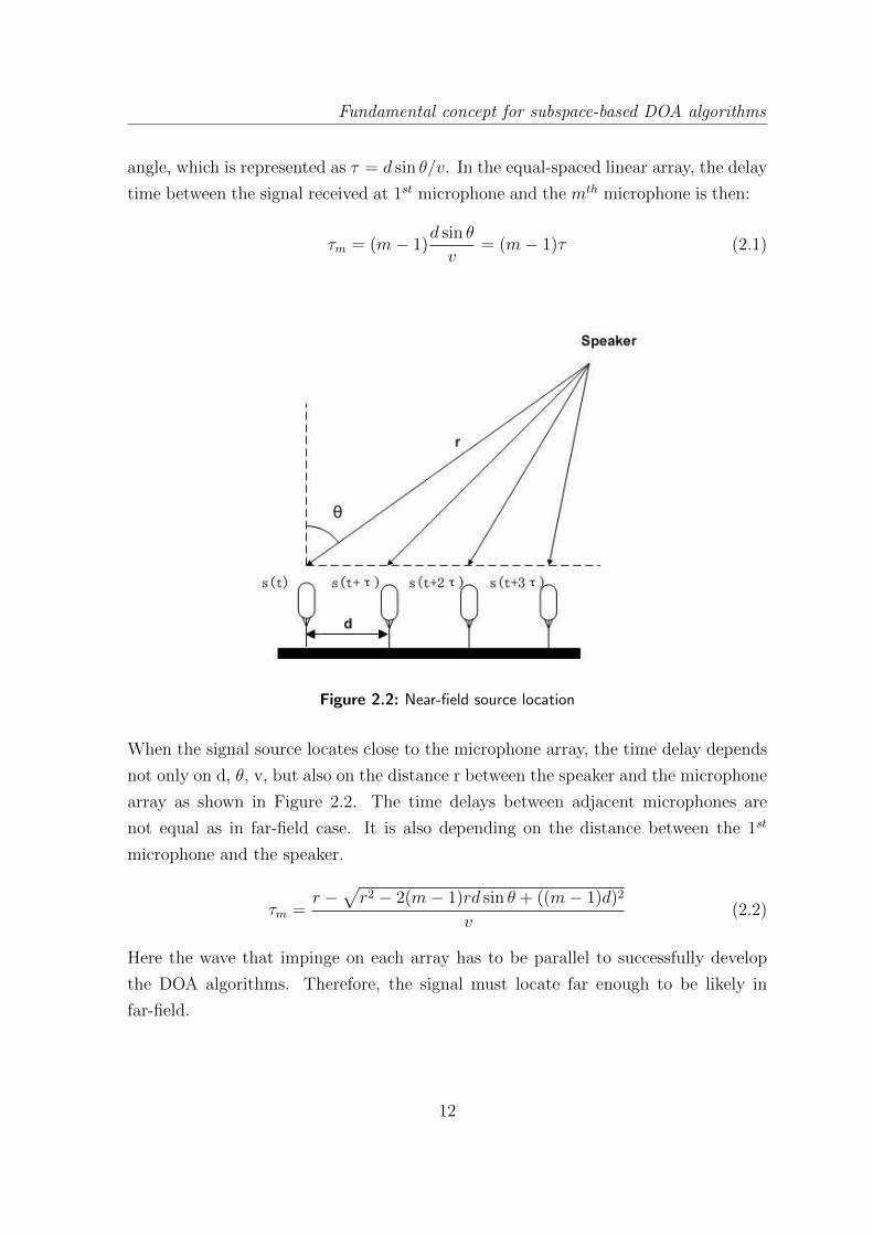
angle, which is represented as τ = d sin θ/v. In the equal-spaced linear array, the delay
time between the signal received at 1st microphone and the mth microphone is then:
τm = (m− 1)d sin θ
v= (m− 1)τ (2.1)
Figure 2.2: Near-field source location
When the signal source locates close to the microphone array, the time delay depends
not only on d, θ, v, but also on the distance r between the speaker and the microphone
array as shown in Figure 2.2. The time delays between adjacent microphones are
not equal as in far-field case. It is also depending on the distance between the 1st
microphone and the speaker.
τm =r −
√r2 − 2(m− 1)rd sin θ + ((m− 1)d)2
v(2.2)
Here the wave that impinge on each array has to be parallel to successfully develop
the DOA algorithms. Therefore, the signal must locate far enough to be likely in
far-field.
12
Fundamental concept for subspace-based DOA algorithms
2.1.2 Narrowband Assumption
Besides that the signals have to locate far enough to make a planar wavefront on the
microphone array, the classic DOA algorithm also requires the signal to be narrowband.
Assuming that s(t) is the signal source, then the received signal at the microphone
could be represented as
s(t) = αs(t− τ) (2.3)
where α is the attenuation factor and τ is the delay time difference. Here, the noise is
not taken into consideration. The signal that received at microphones is not distorted
by the noise. In the frequency domain, the time delay directly translates to a phase
shift.
s(r − τ)↔ S(f)e−j2πfτ (2.4)
Assumed that the signal has centre frequency fc, and the bandwidth is much less
compare with the centre frequency.
fc −B
2≤ f ≤ fc +
B
2when B � fc
Then f could be approximately equal to the centre frequency and phase-shift is ap-
proximately constant over all the bandwidth. The above equation could be rewritten
as:
S(f)e−j2πfcτ ≈ S(f)e−j2πfτ ↔ s(t)e−j2πfcτ (2.5)
Now, the phase shift is not depending on signal frequency. Only the time delay
decides the value of the phase difference. In certain array geometry, the time delay
received at each microphone varies when the signal emits from different direction. In
this thesis, only ULA and UCA array geometries will be considered. Then the DOA
information could be extracted from the phase difference. Therefore, the narrowband
approximation has to be fulfilled at first for the signal sources:
s(t− τ) ≈ s(t)e−j2πfcτ (2.6)
13

Fundamental concept for subspace-based DOA algorithms
2.2 Array Constructures
In this sections, the main array constructures that used throughout this thesis will
be presented, which are Uniform Linear Array (ULA) and Uniform Circular Array
(UCA). A lot of work has been investigated in the ULA already. Almost all the classic
DOA algorithms are implemented on this array constructure. Recently, UCA array
constructure gets more and more attention, since it has some advantages compare to
the ULA.
2.2.1 Uniform Linear Array (ULA)
Consider a ULA consisting of N identical and omni-directional microphones that are
aligned and equal-spaced allocate on a line. The distance between the adjacent micro-
phones is denoted as d. In the noise-free environment, the signal that impinging on
the leftmost sensor from the far-field source is define as s(t). Then, the signals that
impinge on the other sensors are just a delay version of the first one.
si(t) = s(t− τi) (2.7)
Where τi is the relative delay time between ith sensor and the first one.
Figure 2.3 shows a ULA that contains N microphones and a narrowband signal source
is emitting from far-field. The waves that impinge on each array is approximately
parallel. The angle between the source and the line perpendicular to the ULA is
determined as the directional of arrival. It is denoted as θ. Then the delay at nth
microphones is presented as:
τ = (n− 1)d sin θ
v(2.8)
14

Fundamental concept for subspace-based DOA algorithms
Figure 2.3: Uniform Linear Array
Spatial Aliasing
For linear array, the DOA estimation is only reliable in one side detection. In another
word, the phase difference between any pair of microphone should not be more than
π. The reason is that if the phase difference larger than pi, the source which gives the
phase delay φ will be the same as the one with 2π − φ. Then it cannot tell whether
the signal is coming from the front side of the microphone array or the back side. This
kind of the affect is called spatial aliasing, which is not expected. To avoid the spatial
aliasing, the phase difference between adjacent microphones should be restricted into
π:
|2πfd sin θ
v| ≤ π (2.9)
The wavelength λ could replace the division between the speed and the signal fre-
quency. The minimum wavelength is decided by the maximum frequency of the sig-
nal.
λmin =v
fmax
(2.10)
After substitution, the above equation is written as
|2πfd sin θ
v| ≤ π ⇒ d ≤ λ
2|sin θ|and |sin θ| ≤ 1 (2.11)
15
Fundamental concept for subspace-based DOA algorithms
Considering the worst case when θ = 90◦, then |sin θ| = 1 and d should be less or
equal than half of the wavelength. Then the maximum distance could be taken to
avoid spatial aliasing is
dmax =λmin
2(2.12)
In reality, the distance could be adjusted according to maximum signal frequency.
Normally the frequency of the speech signal is from 300Hz to 3000Hz. Suppose the
maximum frequency is 4kHz, then the minimum distance between the adjacent mi-
crophones should be
dmax =1
2· 343m/s
4000Hz≈ 0.043m
Now considering that d signal sources from different angles impinge on the ULA micro-
phone array si(t), 1 ≤ i ≤ d, the overall signal and noise received by the mth element
at time t can be expressed as:
xm(t) =d∑i=1
si(t− τm) + nm(t)
To differentiate the pure signal generated by the source and the noise-corrupted signal
received at each microphone, the latter is called data and denoted by the symbol x.
The steering vector is defined by collecting the phase difference of the signal at each
microphone.
ai(θ) =[1 e−j2πfτ1 . . . e−j2πfτN
]=[1 e−j2πf
dv
sin θ . . . e−j2πf(N−1)d
vsin θ] (2.13)
This equation shows the steering vector that forms the column of the steering matrix
A.
A =[a(θ1) . . . a(θi) . . . a(θd)
]
=
1 . . . 1 . . . 1
e−j2πfdv
sin θ1 . . . e−j2πfdv sin θi . . . e−j2πf
dv
sin θd
. . . . . . . . . . . . . . .
e−j2πf(N−1)d
vsin θ1 . . . e−j2πf
(N−1)dv sin θi . . . e−j2πf
(N−1)dv
sin θd
(2.14)
16

Fundamental concept for subspace-based DOA algorithms
Then the data at microphone array as matrix form could be expressed as:
X = AS + N (2.15)
2.2.2 Uniform Circular Array (UCA)
In last section, the basic structure of the ULA was introduced and single ULA can only
provide a −90◦ to 90◦ angle detection. It cannot give a solution to scenarios where 360◦
of azimuth coverage and a certain degree of source elevation information are required.
In these scenarios, an good alternative is to apply a circular structure, which is called
Uniform Circular Array (UCA). Figure 2.4 shows an example that microphones were
uniformly distributed on circumference of the UCA. The microphones are assumed to
be identical and omni-directional.
Figure 2.4: Uniform Circular Array
Consider a UCA with N sensors and radius r. If the center point of the UCA is
taken as the reference point, a narrowband signal with wavelength λ arriving at nth
microphone from azimuth angle φ ∈ [−π,+π] and elevation angle θ ∈ [0, π/2] causes
a phase difference, which is equal as
ϕm = kr sin θ cos(φ− 2πn− 1
N), where k =
2π
λ
17

Fundamental concept for subspace-based DOA algorithms
Here k is called wave number.Then the steering vector at nth microphone could be
formed as
an(θ, φ) = exp[jkr sin θ cos(φ− 2πn− 1
N)] (2.16)
Assuming that ζ = kr sin θ and γ = 2π(n−1)/N , n = 1, 2, . . . , N . The steering vector
can also be written as:
an(θ, φ) = exp[jζθ cos(φ− γ0), jζθ cos(φ− γ1), . . . , jζθ cos(φ− γN)] (2.17)
The equation shows that the phase shifting at each microphone is not linear indepen-
dent anymore. The steering vector is no more in Vandermonde structure. Suppose
the UCA receives d narrowband signals s1(t), s2(t), . . . , sd(t), the steering vector will
be a N × d matrix:
A =
a1(θ1, φ1) a1(θ2, φ2) . . . a1(θd, φd)
a2(θ1, φ1) a2(θ2, φ2) . . . a2(θd, φd)
. . . . . . . . . . . .
aN(θ1, φ1) aN(θ2, φ2) . . . aN(θd, φd)
(2.18)
Comparison between ULA and UCA
After the introduction of both array constructures, two array manifolds are formed.
The value of array manifold in ULA is unique when the azimuth angle is restricted
between −90◦ and 90◦. The value of the array manifold in UCA is unique when the
signal is coming from the upper surface of the microphone array, which dedicates
that the azimuth angle should be within −180◦ to 180◦ and the elevation angle is
restricted from 0 to 90◦. Therefore, using UCA gives a larger detectable range than
using ULA.
Besides that the UCA has 360◦ detectable azimuth angle, another advantage is
that it require much less space to construct UCA than ULA. To avoid spatial aliasing,
the maximum distance between the adjacent microphones is 4.5cm. For a ULA which
contains 8 microphones, the total length is equal to 36cm. But for a UCA that also
contains also 8 microphones, the required diameter is only 9cm. Therefore, it requires
18
Fundamental concept for subspace-based DOA algorithms
much less space to implement the algorithm on a UCA than a ULA. In practice, some
hardware is very sophisticated won’t leave much space to place a big array. In these
situation, UCA will be a prior than ULA.
2.3 Spatial Covariance Matrix
Covariance matrix is widely used in DOA algorithms. Many DOA estimation
algorithms basically extract the information from this array data covariance matrix
first. It is fundamental step for the DOA estimation algorithms.
In the real world, the signals received by the array elements are noise-corrupted.
Normally, the noise at each sensor is uncorrelated and the signal should be correlated
since they are originated from the same source. The DOA information could be
effectively extracted via this property. The spatial covariance matrix is defined as
[9]
Rxx = E{x(t)xH(t)} (2.19)
The degree of the covariance matrix is up to the number of sensors. The larger the
number of sensor is, the higher order of the covariance matrix will be. In practice,
the exact covariance matrix of Rxx is difficult to find due to the limit number of the
data sets. Therefore, an estimation is made by taking N samples of x(tn), 1 ≤ n ≤ N .
Using X to represent x(t) in matrix form, the estimation of the data covariance matrix
could be calculated by the following.
Rxx ≈ Rxx =1
N
N∑n=1
x(tn)xH(tn) (2.20)
In matrix form:
Rxx =1
NXXH (2.21)
The estimated covariance matrix is used in all the classic DOA algorithms.
19

Fundamental concept for subspace-based DOA algorithms
2.4 Subspace-based Technique
All the DOA algorithms based on subspace technique rely on the followings properties
of the spatial covariance matrix Rxx.
• the eigenvectors of the covariance matrix could be partitioned into two spaces,
which are named signal subspace and noise subspace
• the steering vector is corresponding to the signal subspace
• the signal subspace and noise subspace could be distinguished by the eigenvalues
of the covariance matrix
• the spanned signal subspace is orthogonal to the spanned noise subspace
2.5 Decomposition Methods
In linear algebra, both the eigenvalue decomposition (EVD) and the singular value
decomposition are (SVD) the factorization of a matrix into a canonical form. Then
the matrix could be represented in terms of its eigenvalues and eigenvectors. The EVD
can only be applied for the square matrix, which could be written as:
R = QΛQH =[Qs Qn
] [Λs 0
0 Λn
] [Qs Qn
]H(2.22)
The eigenvalues of R are listed in descending order λ21, λ
22, . . . , λ
2d, . . . , λ
2N , then
λ2i ≥ λ2
i+1 for i = 1, 2, . . . , d − 1 and λ2d ≥ λ2
d+1 = . . . = λ2N = σ2. The matrix
Q is partitioned into an N × d matrix Qs whose columns are the d eigenvectors
corresponding to the signal subspace, and an N × (N − d) matrix Qn whose columns
corresponding to the noise eigenvectors [10] [11] [12]. The matrix Λ is a diagonal
matrix that is partitioned into two diagonal matrices (Λs and Λn). The diagonal
elements of d × d Λs are corresponding to the signal eigenvalues. The diagonal
elements of (N − d) × (N − d) Λn are corresponding to the noise eigenvalues, which
could be written as identity matrix σ2I(n−d)×(n−d). σ2 is simply equal to the power of
the noise.
20

Fundamental concept for subspace-based DOA algorithms
An alternative decomposition method to find the eigenvectors of the spatial co-
variance matrix could be involved by using the data matrix X directly. This
decomposition scheme is called singular value decomposition. Suppose the data
matrix X contains n samples of data at N sensors. The n × N matrix X could be
decomposed by SVD:
X = UΣVH (2.23)
Both decomposition methods are able to extract the signal and noise subspaces. The
SVD decomposition method is comparatively more stable than EVD method. For
simulation and hardware implementation in later chapter, SVD is chosen as the de-
composition method.
21

Chapter 3Classic subspace-based DOA Methods
In this chapter, the algorithms of subspace DOA detection (MUSIC and ESPRIT) will
be summarized. Both of them are the most widely used subspaces DOA estimation
algorithms nowadays. A lot of work was investigated in the ULA (Uniform Circular
Array) at first. Recently, people are more focusing on the DOA estimation on the
UCA (Uniform Circular Array). The reason is that UCA provides 360◦ azimuth
detectable range and the hardware requires less space.
The idea and concept of MUSIC and ESPRIT will be introduced which are
normally applied for ULA. The steering vector in ULA has the Vandermonde
structure. In UCA, a phase mode excitation beamforming matrix is used to make
the steering vector to be Vandermonde-like. Then the DOA algorithms similar
as the MUSIC and ESPRIT algorithms , which are called UCA-RB-MUSIC and
UCA-ESPRIT, could be implemented.
The word ’classic’ here requires that signal source should be narrowband. In
addition the signal should locates far enough that the wavefront received at the
microphone array is approximately planar. These two assumptions has been already
discussed in the previous chapter.
22

Classic subspace-based DOA Methods
3.1 MUSIC (Multiple Signal Classification)
In 1977 Schmidt exploited the measurement model in the case of sensor arrays of
arbitrary form. Later he accomplished this by first deriving a complete geometric
solution in the absence of noise, then cleverly extending the geometric concepts to
obtain a reasonable approximate solution in the presence of noise. The resulting
algorithm was called MUSIC (Multiple SIgnal Classification) and has been widely
studied. [4]
Assuming the steering vector of the microphone array is A, then the input
covariance matrix is
Rxx = ARssAH + σ2IN (3.1)
where Rss is the signal correlation matrix, σ2 is the noise common variance, and IN
is the identity matrix with rank N. Suppose the eigenvalues of Rxx are {λ1, . . . , λN},which leads:
|Rxx − λiIN | = 0
|ARssAH + σ2IN − λiIN | = 0
(3.2)
Assume the eigenvalues of the ARssAH are ei,then
ei = λi − σ2 (3.3)
A is the steering vector of a microphone array which are linearly independent. It has
full column rank and the signal correlation matrix Rss is non-singular as long as the
incident signals are not highly correlated.
When the number of incident signal d is less than the number of microphones
N. The eigenvalues could determine the signal subspace and noise space. The steering
vector is corresponding to the signal subspace. As discussed before, the signal
subspace is orthogonal to the noise subspace. Then such a relation is formed as:
{a(θ1), . . . , a(θd)}︸ ︷︷ ︸steering vector
⊥ {λd+1, . . . , λM}︸ ︷︷ ︸noise-subspace
(3.4)
23

Classic subspace-based DOA Methods
This tells that one can estimate the signal subspace by finding the steering vectors,
which are orthogonal to the N × d eigenvectors corresponding to the noise subspace.
In another word, when the steering vectors lie in the signal subspace, the θ is equal
to the true DOAs. Hence by through all possible array steering vectors to find those
that are perpendicular to the noise space, the DOAs can be determined. Assuming
Pn represents the matrix containing the noise subspace:
Pn = {λd+1, . . . , λN}
Since the steering vectors corresponding to the signal subspace are orthogonal to the
noise subspace. aH(θ)PnPHn a(θ) = 0 for θ = θi corresponding to a DOA of an incident
signal. MUSIC spectrum is constructed by taking the inverse of aH(θ)PnPHn a(θ):
PMUSIC =1
aH(θ)PnPHn a(θ)
(3.5)
When there is d incident signal impinging on the microphone array, there will be d
largest peaks showing in the MUSIC algorithm. The DOAs could be obtained by
taking the corresponding angles that have the highest peaks.
24

Classic subspace-based DOA Methods
3.2 ESPRITEstimation of Signal Parameters via Rotational Invariance Techniques
Although MUSIC was the first of the super-resolution algorithm to detect the DOA
of the narrowband signal with additional noise, there are some limitations including
the fact that the complete knowledge of the array manifold is required. That means
the algorithm have to search for all the spatial space (form -90◦ to 90◦ in ULA) to get
the result by applying the MUSIC algorithm for each space. Additional peak search
algorithm has to be applied afterward to find DOA, which increases computation
complexity. To solve the complex computation problem in the MUSIC algorithm,
an algorithm called ESPRIT which is also based on signal subspace technique was
introduced by Richard Roy and Thomas Kailath in 1989.
In the report of the Richard and Thomas [5], the ESPRIT retains the features
of arbitrary array of sensors. But to achieve a significant reduction in computation
complexity, the doublet structure of sensor array has to be fulfilled. The elements in
each doublet have identical sensitivity patterns and are translationally separated by
a known constant displacement vector ∆.
Using doublet structure is to separate the sensor array into two identical sub-
arrays. In the ULA microphone array, difference choice could be done to select two
subarrays. Assume the first subarray is X, the second is Y. The signal received at the
ith sensor on each subarray can then be express as:
xi(t) =d∑
k=1
sk(t)ai(θk) + nxi(t) (3.6)
yi(t) =d∑
k=1
sk(t)ejω0∆ sin θk/vai(θk) + nyi(t) (3.7)
θk is the direction of arrival of the kth source.
∆ is the distance between the doublet sensors.
Combining the outputs of each sensor in each subarray, the receiver data vectors could
25

Classic subspace-based DOA Methods
be written as the following:
x(t) = As(t) + nx(t) (3.8)
y(t) = AΦs(t) + ny(t) (3.9)
s(t) is the d×1 vector of impinging signals (wavefronts) that observed at the reference
sensor of subarray Zx. Φ is diagonal d × d matrix of the phase delays between the
doublet sensors for the d wavefronts, could be given by
Φ = diag{ejγ1 , . . . , ejγ1} (3.10)
where γd = ω0∆ sin θk/v. Defining the total array output as z(t), which is just simply
to combine the two subarray outputs, is represented by
z(t) =
[x(t)
y(t)
]= As(t) + nz(t) (3.11)
where A =
[A
AΦ
], nz(t) =
[nx(t)
ny(t)
].
The structure of A is to imply that the diagonal matrix Φ could be obtained without
the knowledge of A (steering vector). This is the main core of the ESPRIT algorithm
that reduces the computation complexity compare with the MUSIC algorithm.
As the same approach of MUSIC algorithm, ESPRIT requires that N-dimensional com-
plex vector space CN×N of received snapshot vectors should be separated into orthog-
onal subspaces (signal subspace and noise subspace) via an eigenvalue-decomposition
of the covariance matrix Rzz.
Rzz = E[z(t)zH(t)] = ARssAH + σ2I (3.12)
Rss is the covariance matrix of the emitter signals, σ2 and is the noise variance at each
sensor. The covariance Rss is assumed to be full rank (no unity correlated signals)
and the columns of A are assumed to be linearly independent. The subarray manifold
is assumed to be unambiguous (no spatial aliasing).
26

Classic subspace-based DOA Methods
The eigenvalue-decomposition of RZZ has the form:
RZZ =M∑i=1
λieieHi = EsΣsE
Hs + σ2EnE
Hn (3.13)
Where the span of the d eigenvectors Es = {e1, . . . , ed} defines the signal subspace, and
En = {ed+1, . . . , eN} span the noise subspace which are the orthogonal complement
of the signal subspace. All subspace techniques are based on the observation that
span{Es} = span{A}. This implies that there exists a full rand matrix T ∈ Cd×d,
which satisfied Es = AT. Defining
Ψ = TΦT−1 (3.14)
Then Es =
[E0
E1
]=
[A
AΦ
]T .
E0 and E1 are the signal subspaces for subarray 0 and subarray 1. The rela-
tion between the E0 and E1 is
E1 = E0T−1ΦT = E0Ψ (3.15)
The parameter of interest is the eigenvalues of the operator Ψ that maps E0 onto E1
In practice there is no operator that exactly satisfied with above formula, because
both E0 and E1 will be estimated with errors. Therefore a total least square (TLS) is
applied to estimate the operator .
A matrix was define as:
F =
[F0
F1
]∈ Cd×d (3.16)
To minimize the V =∣∣∣[E0 | E1
]F∣∣∣2F
with FF−1 = I, F could be either achieved by
calculate the right singular vector of[E0 | E1
]and get the d smallest singular values,
or get the d smallest eigenvalues of[E0 | E1
] [E0 | E1
]. After determining the F, the
estimate of the operator Ψ could be done by
ΨES = −F0F−11 (3.17)
27
Classic subspace-based DOA Methods
3.3 Phase Mode Excitation
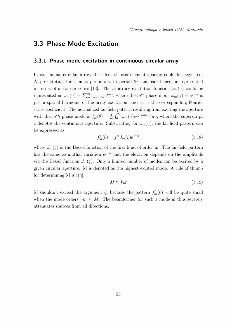
3.3.1 Phase mode excitation in continuous circular array
In continuous circular array, the effect of inter-element spacing could be neglected.
Any excitation function is periodic with period 2π and can hence be represented
in terms of a Fourier series [13]. The arbitrary excitation function ωm(γ) could be
represented as ωm(γ) =∑∞
m=−∞ cmejmγ, where the mth phase mode ωm(γ) = ejmγ is
just a spatial harmonic of the array excitation, and cm is the corresponding Fourier
series coefficient. The normalized far-field pattern resulting from exciting the aperture
with the mth phase mode is f cm(θ) = 1m
∫ 2π
0ωm(γ)ejζ cos(φ−γdγ, where the superscript
c denotes the continuous aperture. Substituting for ωm(γ), the far-field pattern can
be expressed as:
f cm(θ) = jmJm(ζ)ejmφ (3.18)
where Jm(ζ) is the Bessel function of the first kind of order m. The far-field pattern
has the same azimuthal variation ejmφ and the elevation depends on the amplitude
via the Bessel function Jm(ζ). Only a limited number of modes can be excited by a
given circular aperture. M is denoted as the highest excited mode. A rule of thumb
for determining M is [14]:
M ≈ k0r (3.19)
M shouldn’t exceed the argument ζ, because the pattern f cm(θ) will be quite small
when the mode orders |m| ≤ M . The beamformer for such a mode m thus severely
attenuates sources from all directions.
28

Classic subspace-based DOA Methods
3.3.2 Phase mode excitation in uniform circular array
Considering the phase mode excitation of an N element UCA, the normalized beam-
forming weight vector that excites the array with phase mode m is :
wHm =1
N[ejmγ0 , ejmγ1 , . . . , ejmγN−1 ]
=1
N[1, ej2πm/N , . . . , ej2πm(N−1)/N ]
(3.20)
The array pattern f sm(θ) is then equal to:
f sm(θ) = wHma(θ) =1
N
N−1∑n=0
ejmγnejζcos(φ−γn) (3.21)
For mode orders|m| < N , the array pattern can be expressed as:
f sm(θ) = jmJm(ζ)ejmφ +∞∑q=1
(jqJq(ζ)e−jqφ + jhJh(ζ)ejhφ) (3.22)
where g = Nq − m and h = Nq + m. The first term in equation is called principle
term, which is identical to the far-field pattern for the continuous aperture case. The
remaining terms are called residual terms, which come up due to the sampling of
the continuous aperture. To make the principal term to be the dominant one, the
condition N > 2|m| has to be satisfied. The highest mode of the phase excitation is
M, and therefore the number of microphones should be N > 2M . In this case, the
contribution of the residual terms is small enough to be ignored. For the development
of UCA-RB-MUSIC and UCA-ESPRIT algorithms, only the principal terms is taken
into the consideration. The array patterns of UCA is then identical to those for the
continuous circular apertures. Using the property Js−m = (−1)mJm(ζ) of the Bessel
function, the UCA array pattern for mode m can be expressed as:
f sm(θ) ≈ j|m|J|m|(ζ)ejmφ (3.23)
With this background on phase mode excitation of UCA, it can be proceed to develop
the UCA-RB-MUSIC and UCA-ESPRIT algorithms.
29

Classic subspace-based DOA Methods
3.3.3 Beamforming Matrices and Manifold Vectors
Beamforming Matrices are employed to make the transformation from element space
to beamspace [15]. The beamspace transformation FHa(θ) = b(θ) maps the UCA
manifold vector a(θ) onto the beamspace manifold b(θ).
In this section three phase mode excitation based beamformer that synthesize
beamspace manifolds are developed. These beamformers are denoted FHe , FH
r and
FHu . The corresponding beamspace manifolds are ae(θ), ar(θ) and au(θ). The
subscripts e, r, u stand for even, real-valued and UCA-ESPRIT respectively. All
three beamformers are orthogonal that satisfies FHF = 1. An orthogonal matrix V
is defined as
V =√N [w−M
... . . ....w0
... . . ....wM ] (3.24)
The vector wHm defined in Eq (3.20) that excites the UCA with phase mode m, leading
to pattern in Eq (3.23). The factor caused by j|m| could be canceled by the corre-
sponding term j−|m| in matrix Cv:
Cv = diag{j−M , . . . , j−1, j0, j1, . . . , j−M} (3.25)
Then the beamformer FHe is defined as
FHe = CvV
H (3.26)
The beamspace manifold synthesized by FHe is thus
ae(θ) = FHe (a(θ)) ≈
√NJ(ζ)v(φ) (3.27)
The azimuth variation of ae(θ) is through the vector v(φ), which is similar to the
Vandermonde form of the ULA manifold vector. The elevation information could be
derived from the form of symmetric amplitude curve through the matrix of Bessel
function.
Jζ = [JM(ζ), . . . , J1(ζ), J0(ζ), J1(ζ), . . . , JM(ζ)] (3.28)
The subscript e on ae(θ) stands for even, because the diagonal part the matrix of
Bessel function are even about the centre element. The beamspace manifold vectors
are centro-Hermitian, which satisfies Iae(θ) = aHe (θ)
30

Classic subspace-based DOA Methods
I is the reverse permutation matrix:
I =
0 0 0 1
0 0 1 0
. . . . . . . . . . . .
1 0 0 0
(3.29)
The matrix contains ones on the anti-diagonal and zeros elsewhere. Another Beam-
former FHr is constructed by pre-multiply FH
e by a matrix WH with centro-Hermitian
characteristic on rows. Multiply the space array manifold with the real-valued beam-
former FHr will result in a real-valued beamspace manifold b(θ), which is defined as
following:
FHr = WHFH
e = WHCvVH (3.30)
b(θ) = FHr a(θ) =
√NWHJζv(φ) (3.31)
Any matrix W, which satisfies IW = W , will get a real-valued beamspace manifold
b(θ). Matrix W is constructed that FHr synthesizes theM ′ = 2M+1 beams f(ζ, φ−αi),
where f(ζ, φ) is the basic beampattern. Here αi = 2πi/M ′, i ∈[−M M
]are the
azimuth rotation angles. This choice of rotation angles makes W unitary, which keeps
that the beamformer FHr has orthogonal property.
W =1√M ′
[v(α−M)... . . .
...v(α0)... . . .
...v(αM)] (3.32)
With W as above, the basic beampattern is just the sum of the components of ae(θ),
which is f(ζ, θ) = NM ′
[J0(ζ) + 2∑M
m=1 JM(ζ) cos(mφ)]. The beamformer FHr thus
synthesizes the M ′ = 2M + 1 dimensional real-valued beamspace manifold
ar(θ) = [f(ζ, φ−α−M), . . . , f(ζ, φ−α−1), f(ζ, φ), f(ζ, φ−α1), . . . , f(ζ, φ−αM)] (3.33)
The last beamformer FHu synthesizes the beamspace manifold au(θ) specially developed
31
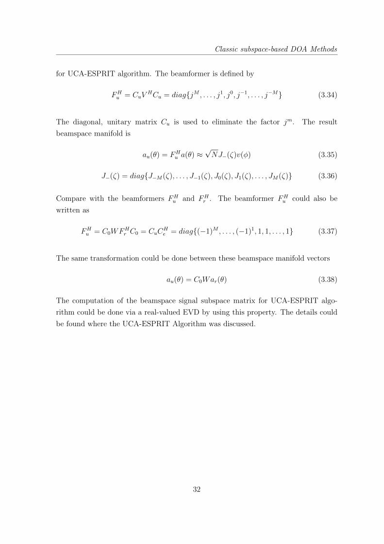
Classic subspace-based DOA Methods
for UCA-ESPRIT algorithm. The beamformer is defined by
FHu = CuV
HCu = diag{jM , . . . , j1, j0, j−1, . . . , j−M} (3.34)
The diagonal, unitary matrix Cu is used to eliminate the factor jm. The result
beamspace manifold is
au(θ) = FHu a(θ) ≈
√NJ−(ζ)v(φ) (3.35)
J−(ζ) = diag{J−M(ζ), . . . , J−1(ζ), J0(ζ), J1(ζ), . . . , JM(ζ)} (3.36)
Compare with the beamformers FHu and FH
r . The beamformer FHu could also be
written as
FHu = C0WFH
r C0 = CuCHe = diag{(−1)M , . . . , (−1)1, 1, 1, . . . , 1} (3.37)
The same transformation could be done between these beamspace manifold vectors
au(θ) = C0War(θ) (3.38)
The computation of the beamspace signal subspace matrix for UCA-ESPRIT algo-
rithm could be done via a real-valued EVD by using this property. The details could
be found where the UCA-ESPRIT Algorithm was discussed.
32

Classic subspace-based DOA Methods
3.4 UCA-RB-MUSIC (Real-Beamspace) Algorithm
The UCA-RB-MUSIC Algorithm employs the real-valued beamformer to transform
the element space to the beamspace. The resulting beamspace data vector is y(t) =
FHr x(t) = Ars(t) + FH
r n(t) , here Ar is vector form of ar(θ). The corresponding
beamspace covariance matrix is
Ry = E[y(t)yH(t)] = BRxBT + σI (3.39)
where Rx is the source covariance matrix in the element space. Since the beamformer
FHr is orthogonal, the noise in the beamspace is white sense as well. Let R denoted as
the real part of the beamspace covariance matrix:
R = Re{Ry} = BRe{Rx}BT + σI (3.40)
The beamspace noise and signal subspaces are calculated by applying a real-valued
EVD on the real part of the beamspace covariance matrix R. Let S and G denote
as the orthonormal matrices that span the beamspace signal and beamspace noise
subspaces. S = [s1, . . . , sd] And G = [gd+1, . . . , gM ] The UCA-RB-MUSIC spectrum
could be calculated by
sb(θ) =1
bT (θ)GGT b(θ)(3.41)
Direction of arrivals of the sources are obtained by search d peaks in the 2D UCA-
RB-MUSIC spectrum.
33

Classic subspace-based DOA Methods
3.5 UCA-ESPRITUniform Circular Array ESPRIT Algorithm
In the last section, the UCA-RB-MUSIC is introduced. Similar as MUSIC algorithm
[4] in the ULA case, it needs to compute the UCA-RB-MUSIC spectrum over all the
azimuth and elevation range, which consume a lot time. In addition, an expensive
spectral peak search algorithm has to be applied to get the DOA estimation. To
avoid these drawbacks that appear in the UCA-RB-MUSIC algorithm, a close-form
algorithm which called UCA-ESPRIT is exploited by Cherian P. Mathews and Michael
D. Zoltowski in 1994 [15], which provides automatically paired source azimuth and
elevation angle estimation. The UCA-ESPRIT algorithm is fundamentally different
from ESPRIT as explained in the last chapter, which is based on the identical subarrays
structure. The UCA-ESPRIT is more developed via the recursive relationship between
Bessel functions. However the implementation steps of the UCA-ESPRIT is similar
as the ones of the normal ESPRIT algorithm applied directly in the element space.
The beamformer FHu is the basis of the development of the UCA-ESPRIT algorithm.
The corresponding beamspace manifold becomes:
au(θ) = FHu a(θ) =
√N
J−M(ζ)e−jMφ
...
J−1(ζ)e−jφ
J0(ζ)
J1(ζ)ejφ
...
JM(ζ)ejMφ
(3.42)
To form the UCA-ESPRIT algorithm, three vectors with the size of Me = M ′ − 2 are
extracted from the beamspace vector, which denoted as a(i), i = −1, 0, 1. They are
simply taken the first, the middle and the last Me elements from the beamspace vector.
Three transforming matrices ∆(i) with i = −1, 0, 1 could be used to pre-multiply with
au(θ) to form the vectors a(i):
a(i) = ∆(i)au(θ) (3.43)
34

Classic subspace-based DOA Methods
with
∆(−1) =
1 0 0 0 0 0
0 1 0 0 0 0...
.... . .
......
...
0 0 0 1 0 0
∆(0) =
0 1 0 0 0 0
0 0 1 0 0 0...
......
. . ....
...
0 0 0 0 1 0
∆(1) =
0 0 1 0 0 0
0 0 0 1 0 0...
......
.... . .
...
0 0 0 0 0 1
The property of the Bessel function, J−m(ζ) = (−1)mJm(ζ), leads that a(1) and a(−1)
have such relationship as:
a(1) = DI(a(−1))∗ (3.44)
where D = diag{(−1)M−2, . . . , (−1)1, (−1)0, (−1)1, . . . , (−1)M}.The manifold vectors (regardless about the sign caused by the Bessel function), a(0)
and ejφa(1) are the same. Then recursive relationship of the Bessel functions is defined
as following:
Jm−1(ζ)Jm+1(ζ) = (2m/ζ)Jm(ζ) (3.45)
It could be applied to match the magnitude components of three vectors, which leads
to:
Γa(0) = µa(−1) + µHa(1)
= µa(−1) + µHDI(a(−1))∗(3.46)
where µ = sin θejφ
Γ =λ
πrdiag{−(M − 1), . . . ,−1, 0, 1, . . . ,M − 1} (3.47)
The partitions of the beamspace DOA matrix also satisfy the above property.
Au = [au(θ1)... . . .
...au(θd)] (3.48)
35

Classic subspace-based DOA Methods
DenotingA(i) = ∆(i)Au with i = −1, 0, 1, the above equation leads to the correlation:
ΓA(0) = A(−1)Φ +DI(a(−1))∗Φ∗ (3.49)
Where Φ = diag{u1, . . . , ud} = diag{sin θ1ejφ1 , . . . , sin θde
jφd}.The beamspace signal subspace matrix Su, that spans R(Au) can be obtained without
performing a complex-valued EVD. The real-valued beamformer FHr is employed and a
real-valued EVD is performed to yield a real-valued signal subspace S that spans R(B).
A real-valued non-singular matrix T was introduced to get S = BT . The beamformer
FHu has such relation with the real-valued beamformer FH
r that FHu = C0WFH
r . Since
the matrix C0 is unitary, thus
Su = C0WS = C0WBT = AuT (3.50)
Applying the same partitioning method expressed above, signal subspace matrices
S(i) = ∆(i)Su with i = −1, 0, 1 are extracted from signal subspace Su. Substituting
S(i) = A(i)T , Eq. (3.49) leads to the relationship in terms of signal subspace matrices:
ΓS(0) = S(−1)Ψ + DI(S(−1))∗Ψ∗ where Ψ = T−1ΦT . Assuming E = [S−1...DIS∗−1] and
Ψ =
[Ψ
Ψ∗
]. The equation could be written in block matrix form:
EΨ = ΓS(0) (3.51)
Under noisy condition, the matrix E and S(0) is replaced by the signal subspace estima-
tions. Then the matrix Ψ that estimates Ψ could be obtained by using a least-square
solution over the equation: EΨ = ΓS(0). The block conjugate structure leads to a sim-
pler LS solution. In the noise-free case, pre-multiply the matrix EH on both left and
right side of Eq. (3.51) , it becomes EHEΨ = EHΓS(0). Substituting the E according
to the assumption, the system will expand as follows:[SH−1
ST−1DI
] [S−1
...DIS∗−1
] [Ψ1
Ψ2
]=
[SH−1
ST−1DI
]ΓS0 (3.52)
After matrix multiplication, to equate the upper and lower blocks of the above equa-
36
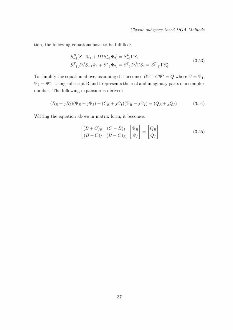
Classic subspace-based DOA Methods
tion, the following equations have to be fulfilled:
SH−1[S−1Ψ1 +DIS∗−1Ψ2] = SH−1ΓS0
ST−1[DIS−1Ψ1 + S∗−1Ψ2] = ST−1DIΓS0 = ST(−1)ΓS∗0
(3.53)
To simplify the equation above, assuming d it becomes BΨ+CΨ∗ = Q where Ψ = Ψ1,
Ψ2 = Ψ∗1. Using subscript R and I represents the real and imaginary parts of a complex
number. The following expansion is derived:
(BR + jBI)(ΨR + jΨI) + (CR + jCI)(ΨR − jΨI) = (QR + jQI) (3.54)
Writing the equation above in matrix form, it becomes:[(B + C)R (C −B)I
(B + C)I (B − C)R
][ΨR
ΨI
]=
[QR
QI
](3.55)
37
Chapter 4Simulation for classic subspace-based DOA
algorithms
In the last chapter, the basic DOA algorithms has been introduced in both ULA and
UCA. In ULA, the normal MUSIC and ESPRIT could be applied. Both algorithms
needs to decomposition the data outputs into two subspaces (signal subspaces and
noise subspaces). The MUSIC algorithm is to find the steering vectors that are
orthonormal to the noise subspaces. The ESPRIT algorithm extracts the DOA
information from the diagonal matrix Ψ. Since two identical subarrays has the
constant displacement ∆, the value of the matrix is only depending on the incident
angles. Both algorithms are basic subspace decomposition. The difference is that the
MUSIC needs information of the noise subspace and the ESPRIT needs the one of
the signal subspaces.
In UCA, via phase mode excitation, difference beamforming matrices are formed to
transform the steering vector from element space to beam space. Then algorithms
UCA-RB-MUSIC and UCA-ESPRIT are applied to estimate the DOAs.
In this chapter, it mainly shows the simulations for all the classic DOA algo-
rithms and analyze the performance of each algorithm by using difference parameter
settings. Here the incident signal is a sinusoidal wave with given frequency, which
38

Simulation for classic subspace-based DOA algorithms
fulfills the assumptions discussed before. At first, some parameters are defined as:
• N: Number of microphones
• D: Number of source
• DOA: directional of arrivals
• SNR: signal-to-noise ratio
By changing one or some of them, simulation will show how these factors affect the
detection result.
39
Simulation for classic subspace-based DOA algorithms
4.1 classic DOA algorithms in ULA
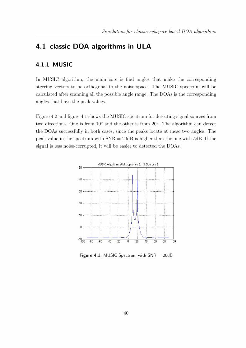
4.1.1 MUSIC
In MUSIC algorithm, the main core is find angles that make the corresponding
steering vectors to be orthogonal to the noise space. The MUSIC spectrum will be
calculated after scanning all the possible angle range. The DOAs is the corresponding
angles that have the peak values.
Figure 4.2 and figure 4.1 shows the MUSIC spectrum for detecting signal sources from
two directions. One is from 10◦ and the other is from 20◦. The algorithm can detect
the DOAs successfully in both cases, since the peaks locate at these two angles. The
peak value in the spectrum with SNR = 20dB is higher than the one with 5dB. If the
signal is less noise-corrupted, it will be easier to detected the DOAs.
Figure 4.1: MUSIC Spectrum with SNR = 20dB
40

Simulation for classic subspace-based DOA algorithms
Figure 4.2: MUSIC Algorithm with SNR = 5dB
Figure 4.3: Error analyze of MUSIC algorithm with SNR = 20dB, N = 8
In MUSIC, in order to get the DOAs, the peaks search algorithms has to be
implemented. The corresponding angle where the pick locates should be close to the
given incident angle. Figure 4.3 shows the deviation between the given DOAs and
the calculated results using MUSIC algorithm when the SNR = 20dB and number
of microphone is equal to 8. The deviation is about 0.1◦ when the incident angle
is between −60◦ and 60◦. It will increase when the incident angle is close to 90◦
41

Simulation for classic subspace-based DOA algorithms
or −90◦. Therefore, the MUSIC will detect the DOA successfully The accuracy is
degraded when the incident angle is high.
In MUSIC algorithm, the number of the signal source should be less than the
number of microphones. The noise subspace needs to be extracted from the
eigen-vector of the array output. The dimension of the eigen-vector is decided by
the number the microphones, which is N × N . The eigen-vector contains both the
signal subspace noise subspace. The first 1st to dth rows are the signal subspace, and
(d+ 1)th to N th rows are the noise subspace. When the number of source is larger or
equal than the number of microphones, there is no noise subspace will be extracted.
Then the MUSIC spectrum is not possible to calculate.
In the ULA, the DOAs of the signal can only be detected from one side of the
microphone array. In another word, the DOAs should be given −90◦ and 90◦.
It cannot distinguish weather the signal emitting from front or the back side the
microphone array.
Figure 4.4: MUSIC Algorithm with θ = 120◦
Figure 4.4 shows the MUSIC spectrum with DOA is equal to 120◦. As it is claimed
that the ULA could only detect DOA of signals from one side of the microphone
42
Simulation for classic subspace-based DOA algorithms
array, 120◦ will become 60◦, which is symmetrical to the microphone array.
4.1.2 ESPRIT
ESPRIT is a close form-DOA detection algorithm. The DOAs will be given directly
after calculation. No peak searching needs to be applied such as in the MUSIC
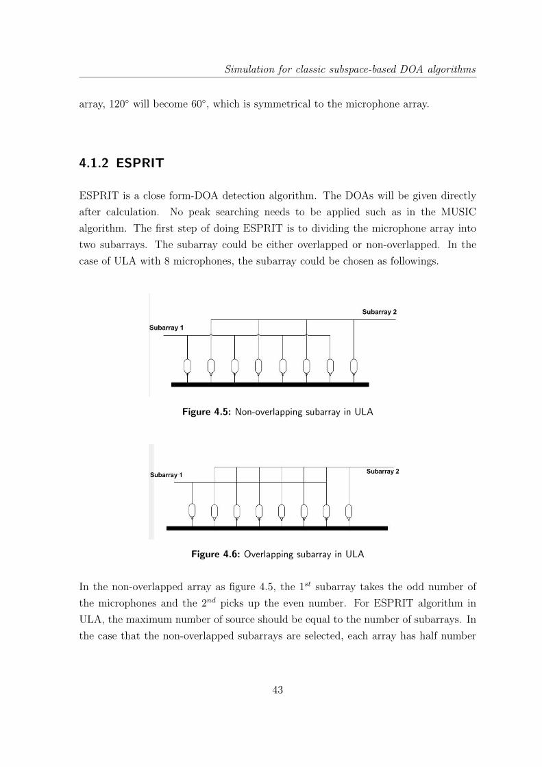
algorithm. The first step of doing ESPRIT is to dividing the microphone array into
two subarrays. The subarray could be either overlapped or non-overlapped. In the
case of ULA with 8 microphones, the subarray could be chosen as followings.
Figure 4.5: Non-overlapping subarray in ULA
Figure 4.6: Overlapping subarray in ULA
In the non-overlapped array as figure 4.5, the 1st subarray takes the odd number of
the microphones and the 2nd picks up the even number. For ESPRIT algorithm in
ULA, the maximum number of source should be equal to the number of subarrays. In
the case that the non-overlapped subarrays are selected, each array has half number
43
Simulation for classic subspace-based DOA algorithms
of the microphones. The maximum number of signal sources is half of the number of
microphones as well.
In the overlapped case, one example is that it chooses the 1st N-1 microphones
as the 1st subarray and from 2nd to N th as the 2nd subarray as shown in figure 4.6.
The maximum number of signal source is increased to N-1. But the trade-off is that
the it take longer to calculate the eigenvector, since the length of the matrix increased
as well when the SVD algorithm is applied.
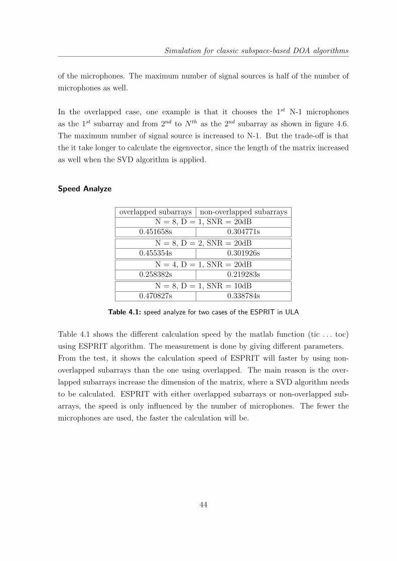
Speed Analyze
overlapped subarrays non-overlapped subarraysN = 8, D = 1, SNR = 20dB
0.451658s 0.304771s
N = 8, D = 2, SNR = 20dB0.455354s 0.301926s
N = 4, D = 1, SNR = 20dB0.258382s 0.219283s
N = 8, D = 1, SNR = 10dB0.470827s 0.338784s
Table 4.1: speed analyze for two cases of the ESPRIT in ULA
Table 4.1 shows the different calculation speed by the matlab function (tic . . . toc)
using ESPRIT algorithm. The measurement is done by giving different parameters.
From the test, it shows the calculation speed of ESPRIT will faster by using non-
overlapped subarrays than the one using overlapped. The main reason is the over-
lapped subarrays increase the dimension of the matrix, where a SVD algorithm needs
to be calculated. ESPRIT with either overlapped subarrays or non-overlapped sub-
arrays, the speed is only influenced by the number of microphones. The fewer the
microphones are used, the faster the calculation will be.
44
Simulation for classic subspace-based DOA algorithms
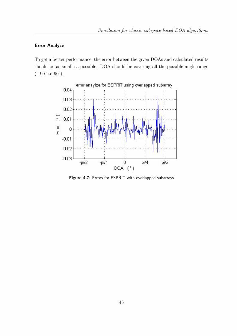
Error Analyze
To get a better performance, the error between the given DOAs and calculated results
should be as small as possible. DOA should be covering all the possible angle range
(−90◦ to 90◦).
Figure 4.7: Errors for ESPRIT with overlapped subarrays
45
Simulation for classic subspace-based DOA algorithms
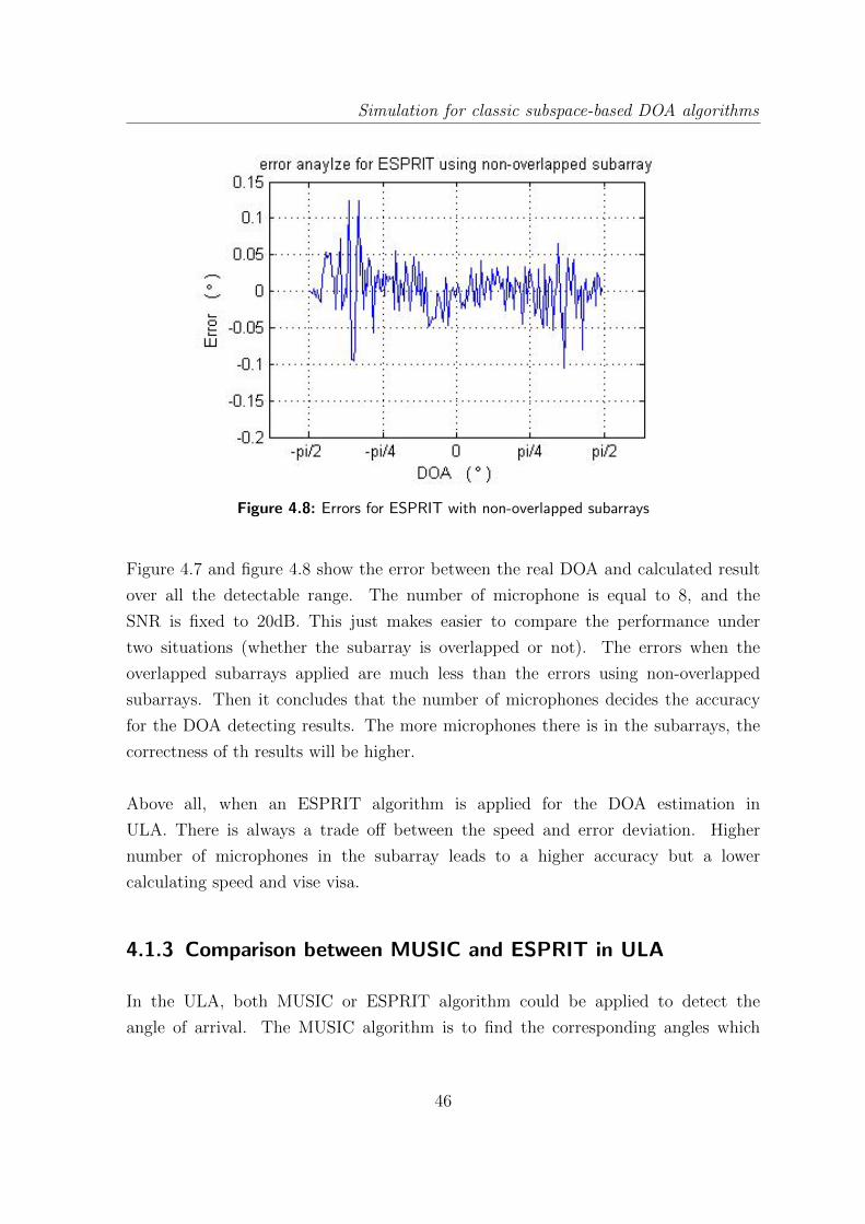
Figure 4.8: Errors for ESPRIT with non-overlapped subarrays
Figure 4.7 and figure 4.8 show the error between the real DOA and calculated result
over all the detectable range. The number of microphone is equal to 8, and the
SNR is fixed to 20dB. This just makes easier to compare the performance under
two situations (whether the subarray is overlapped or not). The errors when the
overlapped subarrays applied are much less than the errors using non-overlapped
subarrays. Then it concludes that the number of microphones decides the accuracy
for the DOA detecting results. The more microphones there is in the subarrays, the
correctness of th results will be higher.
Above all, when an ESPRIT algorithm is applied for the DOA estimation in
ULA. There is always a trade off between the speed and error deviation. Higher
number of microphones in the subarray leads to a higher accuracy but a lower
calculating speed and vise visa.
4.1.3 Comparison between MUSIC and ESPRIT in ULA
In the ULA, both MUSIC or ESPRIT algorithm could be applied to detect the
angle of arrival. The MUSIC algorithm is to find the corresponding angles which
46
Simulation for classic subspace-based DOA algorithms
has the maximum value in the MUSIC spectrum. Before this step, it has to scan
all the possible angle range to get the MUSIC spectrum. Both of them increase the
computation load to get the DOA results. In the contrary, the ESPRIT doesn’t need
any searching procedure.
The deviation between the given DOAs and detect results has been analyzed for both
MUSIC and ESPRIT. No matter whether overlapped subarray or non-overlapped
subarray is applied for ESPRIT, the detection result using ESPRIT is more precise
than MUSIC. Therefore, ESPRIT behaviors much faster and correcter compara-
tively. The only requirement of ESPRIT is that that the subarrays should be identical.
4.2 classic DOA algorithms in UCA
In the last chapter, the theory of doing DOA detection in UCA has been introduced.
Two algorithms which so-call UCA-RB-MUSIC and UCA-ESPRIT are built based on
the phase mode excitation.
4.2.1 simulation result of phase mode excitation
Phase mode excitation is to transform the element space steering vector which has
the Vandermonde structure. The following shows the transformation equation:
f sm(θ) =1
N
N−1∑n=0
ejmγnejζcos(φ−γn) = jmJm(ζ)ejmφ
where wHm = 1N
[ejmγ0 , ejmγ1 , . . . , ejmγN−1 ]
To prove that the beamformer wHm leads to the result as jmJm(ζ)ejmφ, the test case is
made as followings:
• N = 8, number of microphones
• M = 5, maximum phase mode
47

Simulation for classic subspace-based DOA algorithms
• phi = 60 · pi/180, azimuth angle
• theta = 45 · pi/180, elevation angle
• f = 1000, signal frequency
• v = 343, speech speed
• r = 0.045, radius of the array
wHma(θ) jmJm(ζ)ejmφ wHma(θ)− jmJm(ζ)ejmφ
−0.0000 + 0.0040i −0.0000 + 0.0000i 0.0000− 0.0040i
−0.0003− 0.0000i −0.0001 + 0.0003i 0.0001 + 0.0003i
0.0000 + 0.0040i −0.0000 + 0.0000i −0.0000− 0.0000i
0.0206 + 0.0357i 0.0206 + 0.0357i 0.0000 + 0.0000i
0.2418 + 0.1396i 0.2418 + 0.1396i −0.0000 + 0.0000i
0.9168− 0.0000i 0.9168 0.0000 + 0.0000i
−0.2418 + 0.1396i −0.2418 + 0.1396i 0.0000 + 0.0000i
0.0206− 0.0357i 0.0206− 0.0357i 0.0000 + 0.0000i
−0.0000 + 0.0040i 0.0000 + 0.0040i 0.0000 + 0.0000i
−0.0003 + 0.0000i −0.0001− 0.0003i 0.0001− 0.0003i
0.0000 + 0.0040i 0.0000 + 0.0000i −0.0000− 0.0040i
Table 4.2: phase mode excitation
Table 4.2 shows the calculation results of the steering vector from element space to
beamspace with phase mode M = 5. When M > 3, the beamspace steering vector
won’t be identical to the one at element space. To transform the steering vector in
beamspace with little bias, the maximum phase mode M should be restricted in kr.
4.2.2 UCA-RB-MUSIC
Similar as calculate the noise subspace in the normal MUSIC algorithm in ULA, the
UCA-RB-MUSIC algorithm is firstly to calculate the noise subspace in beamspace.
Then the beamspace noise subspace is used to calculate the UCA-RB-MUSIC spec-
trum. The above settings are used again here, but the maximum phase mode is
changed to 3. Then the expected peak of the spectrum should locate at the θ = 45◦,
48
Simulation for classic subspace-based DOA algorithms
and φ = 60◦.
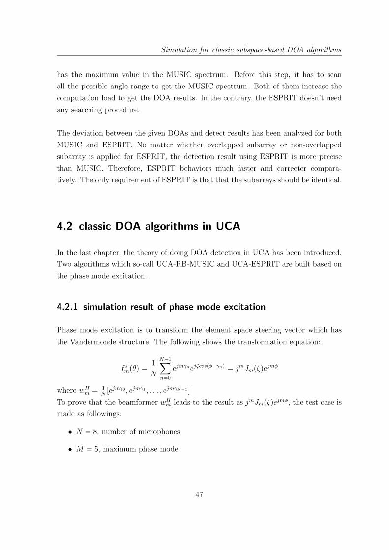
Figure 4.9: 3D plot of UCA-RB-MUSIC spectrum with θ = 45◦, φ = 60◦
Figure 4.9 shows the UCA-RB-MUSIC algorithm in 3D plot. The plot shows one peak
value. To notice the corresponding elevation and azimuth angle of the peak easily, an-
other contour plot is made.
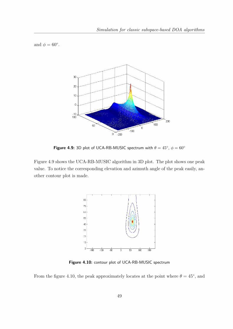
Figure 4.10: contour plot of UCA-RB-MUSIC spectrum
From the figure 4.10, the peak approximately locates at the point where θ = 45◦, and
49
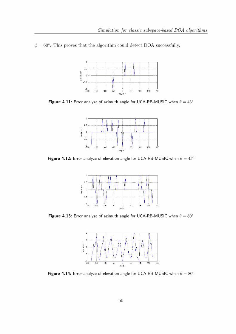
Simulation for classic subspace-based DOA algorithms
φ = 60◦. This proves that the algorithm could detect DOA successfully.
Figure 4.11: Error analyze of azimuth angle for UCA-RB-MUSIC when θ = 45◦
Figure 4.12: Error analyze of elevation angle for UCA-RB-MUSIC when θ = 45◦
Figure 4.13: Error analyze of azimuth angle for UCA-RB-MUSIC when θ = 80◦
Figure 4.14: Error analyze of elevation angle for UCA-RB-MUSIC when θ = 80◦
50

Simulation for classic subspace-based DOA algorithms
Figure 4.11 - figure 4.14 shows the deviations of azimuth and elevation angles when
θ = 45◦ and θ = 80◦. The results shows the UCA-RB-MUSIC algorithm could detect
the azimuth angle correctly. The deviation of elevation angle gets increased when the
given elevation angle changes from θ = 45◦ to θ = 80◦.
4.2.3 UCA-ESPRIT
Like ESPRIT in the ULA, the UCA-ESPRIT is also a close-form DOA detection
algorithm, which gives the DOAs directly after calculation. Normally the detection
results are depending on the following parameters:
• number of microphones (N)
• signal-to-noise ratio (SNR)
• elevation angle (θ)
• azimuth angle(φ)
The main objective is to detect the azimuthal angle correctly. Therefore, the
azimuthal angle is calculated throughout all the detectable range, which is from
−180◦ to 179◦. The detected azimuth angle should be close to the expected value.
The deviations are calculated by subtraction between the calculated results and the
expected values to judge the performance of the algorithm in the different conditions
when the other parameters vary.
Figure 4.15 shows the simulation results of the UCA-ESPIRT when the number
of microphone is 8, signal-to-noise ratio is 20dB, and initial elevation angle is 45◦.
The average azimuthal deviation is about 1◦, and the average deviation for eleva-
tion angle is 5◦. The result of azimuth angle is accurate compare to the elevation angle.
51

Simulation for classic subspace-based DOA algorithms
Figure 4.15: simulation of UCA-ESPRIT 1
52

Simulation for classic subspace-based DOA algorithms
Figure 4.16: simulation of UCA-ESPRIT 2
When the elevation angle is increased to 70◦, the simulation result is shown in
figure 4.16. The average azimuthal deviation now increases, which is about 2◦. And
the average elevational deviation is about 30◦. The results tell that when the azimuth
angle is close to 90◦, the accuracy of the UCA-ESPRIT algorithm will be degraded.
Even that, the deviation of azimuth angle is still not much high, but the elevation
detection is absolutely failed.
53
Simulation for classic subspace-based DOA algorithms
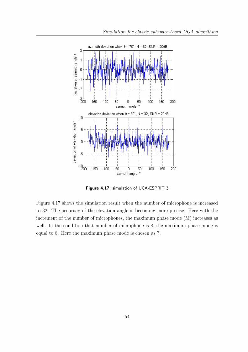
Figure 4.17: simulation of UCA-ESPRIT 3
Figure 4.17 shows the simulation result when the number of microphone is increased
to 32. The accuracy of the elevation angle is becoming more precise. Here with the
increment of the number of microphones, the maximum phase mode (M) increases as
well. In the condition that number of microphone is 8, the maximum phase mode is
equal to 8. Here the maximum phase mode is chosen as 7.
54

Simulation for classic subspace-based DOA algorithms
Figure 4.18: simulation of UCA-ESPRIT 4
When number of microphones is equal to 32, according to the equation introduced
in the previous chapter, the maximum phase mode is 15. Figure 4.18 shows the
simulation results when the maximum phase mode is set to 15. The detected azimuth
and elevation angles are becoming more accurate.
55

Simulation for classic subspace-based DOA algorithms
In figure 4.19, the signal-to-noise ratio is changed to 5dB, which means the signal will
be more corrupted by the noise. Compare with simulation result in figure 4.15, the
simulation results are more accurate in the condition that SNR is high.
Figure 4.19: simulation of UCA-ESPRIT 5
Above all, different situations have been considered. When the elevation angle is
close to 90◦, the calculated elevation is not accurate but the azimuth is still close
to the real DOA. To improve the elevation detection, one method is to increase the
number of microphones. However, the speed of calculated will slow down. For the
final implementation, the main concern is to get the right azimuth angle. Therefore,
the error that occurs in the elevation could be neglected.
All the tests are done to detect the azimuth angle from −179◦ to 180◦. The
deviation between the calculated value and expected one are small. This proves that
56

Simulation for classic subspace-based DOA algorithms
UCA-ESPRIT can detect the azimuth angle successfully in all the situations.
4.2.4 Comparison between UCA-RB-MUSIC and UCA-ESPRIT
Both UCA-RB-MUSIC and UCA-ESPRIT are doing the DOA detection via applying
a beamformer to transform the array output to beamspace. Like the MUSIC
algorithm in ULA, the UCA-RB-MUSIC needs to calculate the spectrum so that
the DOA could be found by searching the location of the peaks. The UCA-ESPRIT
is also a close-form DOA detection algorithm like the ESPRIT in ULA. Avoiding
calculating the spectrum and doing peak search, the UCA-ESPRIT is much faster
compare to the UCA-RB-MUSIC.
4.3 Conclusion
In the ULA, the normal ESPRIT algorithm is applied. The microphone arrays need to
divided into two identical subarray and calculate the rotational transforming matrix.
In UCA, there is no subarray need to separate. In stead, the the signal subspace
vector need to be partitioned into three sub-vectors. Applying the special char-
acteristic of the Bessel function, the azimuth and elevation could be calculated directly.
From the simulation results, the UCA-ESPRIT won’t give a correct elevation
angle when it is close to 90◦. When the number of microphone increases, the results
could be improved. The trade-off is that it takes more time to calculate and more
hardware requirement. Regardless of the elevation, the detection results for the
azimuth angle are quite precise with limited number of microphones. Since the correct
detection for the azimuth angle is the main objective, the UCA-ESPRIT could be
still applied for small number of microphones.
57
Chapter 5Wideband DOA Subspace-based
Algorithms
In the previous chapters, the classic DOA algorithms for both ULA and UCA were
introduced. As mentioned before, these algorithms can only estimate the DOA of
the narrowband sources. The final goal of the implementation is that the system
could detect the DOA for normal speech signals. The speech signal is wideband,
which normally allocates at the frequency band between 300Hz to 3500Hz. Since
the frequency is not narrowband anymore, the classic DOA method cannot directly
applied.
In the previous chapter, it has been proven that only when the bandwidth is
much lower than the centre frequency, it assumes that the signal is narrowband.
Then the phase delay is simply a function of the delay time τ , which only depends
on the DOA and array geometry. Then the DOA information could be extracted by
applying a classic DOA algorithm when a ULA or a UCA is used.
When the signal source is not narrowband anymore, the phase difference doesn’t
rely on the location of source, but also the frequency. To successfully detect the
wideband signal, one approach is done by split the whole band into certain amount
bins. Then the narrownband DOA method could be calculated in each frequency
58
Wideband DOA Subspace-based Algorithms
bin. This method is called incoherent. Another approach is to transform the steering
vector from all frequency bins to one. The translated steering vectors are summed
up to form a coherent covariance matrix. Then any narrowband algorithm could be
applied for the coherent covariance matrix at the reference frequency. This class of
the wideband DOA detection is named coherent. In following sections, these two
main categories of the wideband DOA algorithms will be discussed.
5.1 Incoherent Wideband DOA Algorithm
The incoherent wideband DOA algorithm is to apply the narrowband DOA algorithm
on all the frequency bins and average them [18] [19]. For example, when MUSIC
algorithm is used as the narrowband DOA algorithm, the spectrum at K frequency
bins will be sum up incoherently:
SM =1
K∑i=0
aH(fi, θ)WiWHi a(fi, θ)
(5.1)
Fi: The centre frequency on each frequency bin.
Wi: The estimated noise subspace by applying the MUSIC on the array outputs at
each frequency bin.
K: total number of the frequency bins
The estimated DOA could be found by using a peak search method as normal
MUSIC DOA algorithm does. The corresponding angle at the peak value is the
estimated DOA. The normal structure for the incoherent wideband DOA algorithm
is shown in the figure 5.1.
59

Wideband DOA Subspace-based Algorithms
Figure 5.1: Incoherent Wideband DOA algorithm
The incoherent wideband DOA algorithm provides a good DOA estimation when the
SNR is high and the noise uniformly locates at each frequency bin. In addition, the
computation complexity is depending on the number of the frequency bins. The more
the frequency bins there are, the more complex the computation will be, because each
frequency bins need to perform a MUSIC algorithm once.
To reduce the computation load, it is better to choose certain amount of the
frequency bins than to select all. A FFT (Fast Fourier Transform) algorithm could
be applied to calculate the signal spectrum. Then split the spectrum into different
section and select the one with maximum magnitude. After that, the narrowband
DOA algorithms such as MUSIC, ROOT-MUSIC, ESPRIT, could be used on these
selected frequencies. In the end, the result is taken by averaging the values calculated
at each frequency.
5.2 Coherent Wideband DOA Algorithm
To avoid performing narrowband algorithm on each frequency bins, the coherent wide-
band DOA algorithms was introduced. The idea of the coherent wideband DOA algo-
rithm is to align all the covariance matrices at different frequency bins into one certain
frequency. Then, a narrowband DOA algorithm could be performed only once for the
coherent covariance matrix. Figure 5.2 shows the structure of the coherent wideband
DOA algorithm. The narrowband algorithm shown in the figure use ESPRIT.
60

Wideband DOA Subspace-based Algorithms
Figure 5.2: Coherent Wideband DOA algorithm
The main task for coherent wideband DOA algorithm is to align the signal subspace
from all the frequency bins into one. The alignment is accomplished by a transfor-
mation of a covariance matrix on each frequency bins. After transformation, both
signal and noise subspaces become coherent over the frequency bin. Then any narrow-
band DOA algorithm could be applied on the coherent covariance matrix to calculate
DOA.
5.2.1 Coherent Signal Subspace Method (CSSM)
CSSM was introduced by Wang and Kaveh [20]. In this method, an estimation of the
synthesized covariance matrix is formed via:
Rcom =ku∑i=kl
αiTiRiTHi (5.2)
where αi is the weighting factors, kl and ku are respectively the inferior and superior
limit. Ti is the focusing matrix for frequency fi, which could be derived by calculating
the following minimizing function.
minTi‖A(fr, θr)− TiA(fi, θi)‖ (5.3)
61

Wideband DOA Subspace-based Algorithms
fr is the reference frequency and θr is the focusing angles. The reference frequency
could be randomly chosen in frequency band. To simplifying the Rcom , the weighting
factor is assumed to be 1 over all the frequency bins.
Rcom =K∑i=0
TiRiTHi
=K∑i=0
Ti{A(fi, θf )Rs(fi)AH(fi, θf ) + σ2(fi)}THi
≈ A(fi, θf )K∑i=0
Rs(fi)A(fr, θf ) + σ2(fi)TiTHi
(5.4)
From the equation above, it shows that the CSSM tried to composite all the trans-
formed covariance matrices from all the frequency bins into one. The focusing matrix
Ti transforms the covariance at current frequency to the reference one. The ratio
between the SNR after transformation and the SNR before focusing is denoted as
focusing loss.
g =
tr{R−1n
K−1∑i=0
TiA(fi, θ)RsAH(fi, θ)T
Hi }
tr{K−1∑i=0
A(fi, θ)Rs(fi, θ)AH(fi, θ)}
(5.5)
where Rn is related to the noise covariance matrix after focusing via:
Rn =
K−1∑i=0
σ2(fi)TiTHi
K−1∑i=0
σ2(fi)
(5.6)
The focusing loss will reach the maximum value (g=1) when the TiTHi = I over all the
frequency bins. Assuming the focusing angle θr is determined, the focusing matrix Ti
is found via
minTi‖A(fr, θf )− TiA(fi, θf )‖F (5.7)
62

Wideband DOA Subspace-based Algorithms
For i = ku . . . kl subject to TiTHi = I . The solution for the above minimization
problem is
Ti = ViUHi (5.8)
Ui and Vi are respectively the right and left singular matrices of
A(fr, θf )AH(fi, θf ) (5.9)
The CSSM is robust against low SNR and has high resolution compare with incoherent
method. But the performance is also decided by the focusing angle. To form the
focusing matrix, a preliminary initial estimation angle has to be given. The errors
in the focusing angle cause bias in the DOA estimation. How to get a good initial
estimation of the DOA is a crucial question. In some documentation, it mentions
that a conventional beamformer such as Capon beamformer could be applied to get
the initial estimation of the DOA.
However, the conventional beamformer sometimes doesn’t promise to give an
accurate initial DOA estimation. Therefore, people are looking for some algorithms
that don’t need any preliminary angle.
5.2.2 Robust auto-focusing Coherent Signal-subspace Method
(R-CSM)
In the previous section, the coherent wideband DOA estimation is analyzed. The
conclusion is that the result is affected by the accuracy of the initial DOA estimation
(sometimes called focusing angle). In another word, in order to improve the coherent
wideband DOA estimation, the very first DOA estimation must be as accurate as
possible with a low computation cost. The proposal could be either to perform
narrowband DOA estimation or to use a conventional beamformer. Then, the result
could be optimized by doing CSSM iteratively to reduce the estimation error. But it
is not so effective since the focusing angle is still different from the actually one. To
avoid this, in this section, a new method,so-called R-CSM (Robust auto-focusing Co-
herent Signal-subspace Method) [21], which doesn’t need the initial DOA estimation
is discussed.
63

Wideband DOA Subspace-based Algorithms
In R-CSM, the focusing matrices required in the very first step are calculated
to the following optimization problem.
Tk[0] = arg{minTi
∫ π2
π2
‖Ta(θ, fk)− a(θ, fr)‖2Fdθ} (5.10)
where a(θ, fk) is the array manifold evaluated at the frequency fk. fr is the reference
frequency, θ is the focusing angle, here θ ∈ [−π2
π2] in the ULA case.
As it can be observed, the focusing matrix is not calculated by a given initial
DOA estimation. In stead, it becomes a minimization problem with respect to the
whole possible region. In the ULA, the detectable angle is from −89◦ to 90◦. The
minimization problem could be solved by least square method. The solution to the
problem is given by
Tk[0] = VkUHk (5.11)
where Uk and Vk are respectively the right and left matrices obtained from the singular
value decomposition of the matrix
Qk ,∫ π
2
π2
a(θ, fk)aH(θ, fr)dθ = UkΣV
Hk (5.12)
After running a signal-subspace-based DOA estimation algorithm such as MUSIC,
ESPRIT, a set of possibly reliable initial estimates θ[0] , [θ1[0], θ2[0], . . . , θd[0]] is
available for refinement by subsequent iterations. The new focusing matrix needs to
be firstly calculated by solving
Tk[i] = arg{minTi
d∑l=1
∫ θl+∆i
θl−∆i
‖Tk[i]a(θ, fk)− a(θ, fr)‖2Fdθ} (5.13)
where [θl −∆i θl + ∆i], i ∈ 1, 2, . . ., refers to the new robustness intervals.
Robustness interval defines the region over which the robustness against DOA
estimation errors needs to be mainly concentrated. After first iteration, it is no longer
necessary to focus the array manifold over the whole visible region. It is more effective
64
Wideband DOA Subspace-based Algorithms
to concentrate the spatial space around the initial DOA estimation. It makes more
sense to reduce the robustness boundary after each iteration. One of the possibilities
to realize the reduction of the boundaries is exponential, which obey the following
rule:
θ[i] = [max{−π2, θl −
π
2i},min{π
2, θu +
π
2i}] (5.14)
θl, θu are respectively the largest and smallest DOA estimation from (i − 1)th itera-
tion.
5.2.3 Beamspace Coherent Signal Subspace Method in UCA
In the UCA, the steering vector in the element space needs to be transformed to the
beamspace via phase mode excitation.
f sm(θ) ≈ jmJm(ζ)ejmφ (5.15)
The beamspace steering vector has the same phase shift which depends on the
azimuth angle. The amplitude of each element is the Bessel function which depends
on both the elevation and frequency. To form a matrix that could transform the
beamspace steering vector from one frequency to the reference frequency, the only
part need to be considered is the Bessel function.
To make the Bessel function depends only on the frequency, the elevation an-
gle needs to be pre-defined. Normally, the speaker stays quite far from the UCA,
which leads the elevation is approximately equal to 90◦. Then the focusing matrix in
the beamspace could be calculated as:
Bm = Jm(ζ0)/Jm(ζ) (5.16)
where ζ0 = k0r and ζ = kr.
As introduced before, a beamformer F is used to transform the steering vector
from element space to beamspace. After the focusing the steering vectors from other
frequencies to the reference frequency, the beamspace steering vector needs to be
65
Wideband DOA Subspace-based Algorithms
transform back to element space by pre-multiply the inverse matrix of F. Therefore,
an new matrix Ti could be form as such way that transform the element-space steering
vector directly from one frequency to the reference one:
Ti = F−1BmF (5.17)
The CSSM in UCA is not like the CSSM in ULA that could achieve the focusing loss
ratio equal to 1. Therefore, the SNR before and after focusing are not identical.
66
Chapter 6Simulation for Wideband Subspace-based
DOA Algorithms
In the last chapter, the concept of how to implement the wideband DOA algorithms
has been introduced. There are main two categories to realized the DOA detection
for wideband signals. One is incoherent, which needs to applied the narrowband
algorithms several times. The other is coherent, which needs the narrowband methods
only once. Both methods needs to separate the signal spectrum into sections. The
purpose is to treat each section as narrowband.
In this chapter, the simulation will be presentation to show the performance of
the wideband DOA algorithms. An artificial signal has to be created firstly for the
microphone array output via VPDs (Variable Phase Delay filters ). A frequency
selective algorithm is to select the fundamental frequencies in each section. Then
either the coherent or incoherent methods has to be implemented to estimate the
DOAs.
67
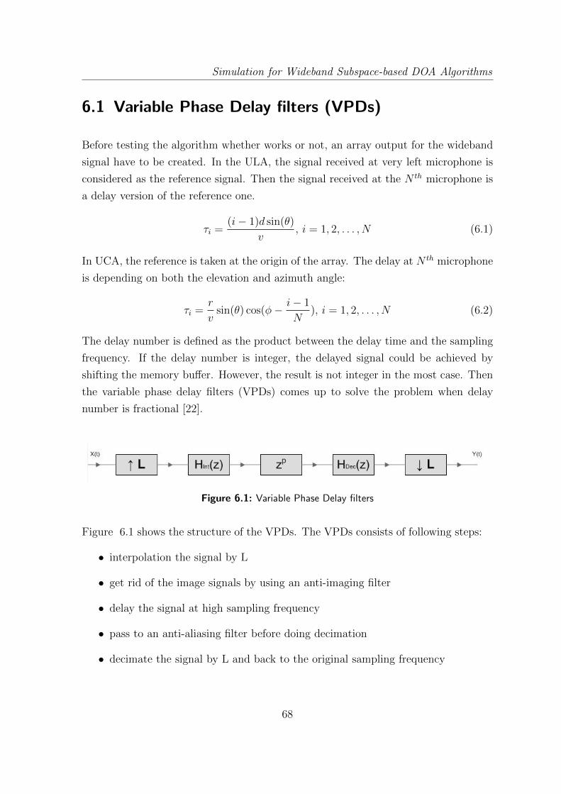
Simulation for Wideband Subspace-based DOA Algorithms
6.1 Variable Phase Delay filters (VPDs)
Before testing the algorithm whether works or not, an array output for the wideband
signal have to be created. In the ULA, the signal received at very left microphone is
considered as the reference signal. Then the signal received at the N th microphone is
a delay version of the reference one.
τi =(i− 1)d sin(θ)
v, i = 1, 2, . . . , N (6.1)
In UCA, the reference is taken at the origin of the array. The delay at N th microphone
is depending on both the elevation and azimuth angle:
τi =r
vsin(θ) cos(φ− i− 1
N), i = 1, 2, . . . , N (6.2)
The delay number is defined as the product between the delay time and the sampling
frequency. If the delay number is integer, the delayed signal could be achieved by
shifting the memory buffer. However, the result is not integer in the most case. Then
the variable phase delay filters (VPDs) comes up to solve the problem when delay
number is fractional [22].
Figure 6.1: Variable Phase Delay filters
Figure 6.1 shows the structure of the VPDs. The VPDs consists of following steps:
• interpolation the signal by L
• get rid of the image signals by using an anti-imaging filter
• delay the signal at high sampling frequency
• pass to an anti-aliasing filter before doing decimation
• decimate the signal by L and back to the original sampling frequency
68

Simulation for Wideband Subspace-based DOA Algorithms
The L and P are respectively the numerator and denominator of the delay number. In
Matlab the interpolation and anti-imaging filter could be done by calling the function
interp, and the decimation including the anti-aliasing filter is done by calling the
function decimate .
Figure 6.2: Artificial Array Output via VPDs in ULA
Figure 6.2 shows the artificial signals that contain the signal outputs from each
microphone in an ULA when the signal locates at 45◦. In the ULA, the distance
between adjacent microphone is identical. This leads the delay between the adjacent
microphone is the same as well.
69
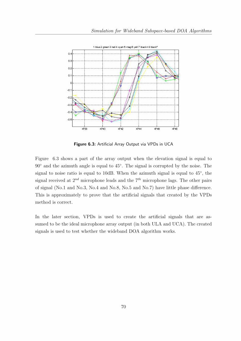
Simulation for Wideband Subspace-based DOA Algorithms
Figure 6.3: Artificial Array Output via VPDs in UCA
Figure 6.3 shows a part of the array output when the elevation signal is equal to
90◦ and the azimuth angle is equal to 45◦. The signal is corrupted by the noise. The
signal to noise ratio is equal to 10dB. When the azimuth signal is equal to 45◦, the
signal received at 2nd microphone leads and the 7th microphone lags. The other pairs
of signal (No.1 and No.3, No.4 and No.8, No.5 and No.7) have little phase difference.
This is approximately to prove that the artificial signals that created by the VPDs
method is correct.
In the later section, VPDs is used to create the artificial signals that are as-
sumed to be the ideal microphone array output (in both ULA and UCA). The created
signals is used to test whether the wideband DOA algorithm works.
70

Simulation for Wideband Subspace-based DOA Algorithms
6.2 Frequency selection
In the narrowband DOA algorithms, the signal consists of only one frequency
component. But for normal speech signal, the spectrum locates from 100Hz to
3500Hz, which is not narrowband anymore. Then to analyze the signal spectrum and
to get the fundamental frequencies will be very necessary. In the most case, the Fast
Fourier Transform (FFT) is used to calculate the spectrum of signal. To reduce the
spectrum leakage, a window has to be applied.
Figure 6.4: Speech signal in frequency domain
In Figure 6.4, it shows the spectrum of the sampled speech signal. It could be noticed
that only some of the frequency components do the main contribution. Selecting the
frequency components that contain the higher values makes more sense to choose the
ones with lower values. The noise is assumed to be white when the signal transmits
through the air. Then if the frequency components with high values are selected,
the corresponding signal-to-noise ratio at the selected frequency is high as well.
Therefore, to calculate the DOA on these frequency components will be more reliable.
71

Simulation for Wideband Subspace-based DOA Algorithms
The approach in this thesis for selecting the fundamental frequency is to split
the whole frequency range into different sections and pick the frequency component
with the highest absolute value in each section. All the selected frequencies should be
sorted descendingly and the components with the higher values are taken into DOA
calculation.
Figure 6.5: Fundamental frequency selection
In Figure 6.5, the frequency components with red color are the fundamental frequency
components which are selected via frequency selection algorithm.
72

Simulation for Wideband Subspace-based DOA Algorithms
6.3 Incoherent wideband DOA algorithms
Now each selected frequency component could be used for narrowband DOA algo-
rithms individually. If the MUSIC algorithm is chosen as the detection algorithm, the
final result is just to sum up the MUSIC spectrum and search the peaks, which is
the same as the one for narrowband detecting. For the ESPRIT algorithm, the result
is achieved by summing up DOAs on each selected frequency and takes the average
value. This kind of approaches that calculate the DOAs individually on each frequency
is called incoherent method.
6.3.1 Incoherent MUSIC in ULA
When the MUSIC algorithm is applied, different MUSIC spectrums are obtained at
different fundamental frequency. After summing up all these MUSIC spectrums, an
synthetical MUSIC spectrum is formed.
Figure 6.6: Incoherent MUSIC in ULA
Figure 6.6 shows the MUSIC spectrum at each selected frequency when DOA= 45◦.
Though the spectrum in yellow color tells the wrong DOA information, the final
73

Simulation for Wideband Subspace-based DOA Algorithms
MUSIC spectrum (in black color) still gives the DOA which is very close to the real
one.
6.3.2 Incoherent ESPRIT in ULA
Since the ESPRIT is a close-form DOA algorithm, it will give the estimated DOAs
directly instead of a spectrum like MUSIC algorithm. The final DOA could be
calculated by averaging the DOAs that are computed at each fundamental frequency.
Incoherent ESPRIT Algorithm with θ = 45◦
Fundamental Frequency (Hz) 375 562.5 1375 1562.5 2437.5Direction of Arrival θi 43.4323◦ 47.1488◦ 47.0296◦ 41.7513◦ 3.4052◦
θ = 35.1914◦
Table 6.1: Incoherent ESPRIT in ULA
Table 6.1 shows the result via the incoherent ESPRIT method. The 3rd row shows the
calculating result using narrowband ESPRIT algorithm on each selected frequency. It
is apparently to be seen that not all the results are close to the real direction-of-arrival
angle. Since the final DOA is obtained by averaging the DOAs calculated on these
frequencies. One detection error would cause the imprecision of the final result.
6.3.3 Comparison between incoherent methods in ULA
For the incoherent method in ULA, the result by applying MUSIC algorithm is much
better than using the ESPRIT algorithm. The MUSIC algorithm is to calculate the
MUSIC spectrum on the selected frequencies and sum up. In the end, the DOA could
be achieved by the peak search on the composed MUSIC spectrum.
The ESPRIT is not like MUSIC algorithm. Since it is a closed-form DOA al-
gorithm, it will give the DOAs directly. In case that the DOA that calculated by
ESPRIT algorithm at one of the selected frequencies is wrong. The correctness of the
74

Simulation for Wideband Subspace-based DOA Algorithms
final DOA will be dramatically degraded, because it is calculated by averaging all the
DOAs calculated from all selected frequency. The conclusion for incoherent method
is that the MUSIC algorithm performs better than the ESPRIT algorithm.
6.3.4 Incoherent UCA-RB-MUSIC
Similar as the MUSIC algorithm in ULA, the UCA-RB-MUSIC is to calculate the
spectrum at first as well. The UCA-RB-MUSIC needs a 2-D search algorithm to find
the peaks. One dimension is corresponding to the elevation angle, and the other is to
the azimuth angle.
Figure 6.7: Incoherent UCA-RB-MUSIC in UCA
Figure 6.7 shows the contour plot of the final UCA-RB-MUSIC spectrum, which
is the summation of the spectrums calculated at the fundamental frequencies.
The x axis and y axis are respectively the azimuth angle and the elevation. The
peak locates at the position where azimuth angle is 45◦ and elevation angle is 60◦.
The real azimuth angle is 45◦ and elevation angle is 90◦. This tells that the al-
gorithm could detect the azimuth angle very accurately, but not for the elevation angle.
75
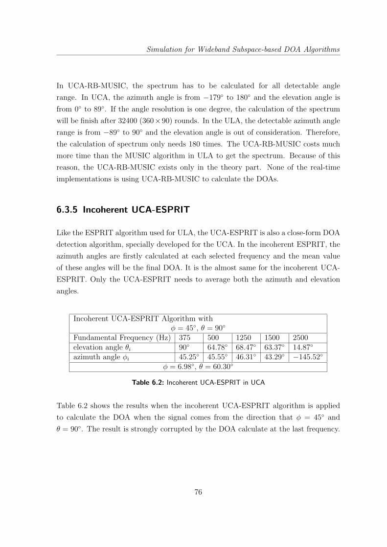
Simulation for Wideband Subspace-based DOA Algorithms
In UCA-RB-MUSIC, the spectrum has to be calculated for all detectable angle
range. In UCA, the azimuth angle is from −179◦ to 180◦ and the elevation angle is
from 0◦ to 89◦. If the angle resolution is one degree, the calculation of the spectrum
will be finish after 32400 (360×90) rounds. In the ULA, the detectable azimuth angle
range is from −89◦ to 90◦ and the elevation angle is out of consideration. Therefore,
the calculation of spectrum only needs 180 times. The UCA-RB-MUSIC costs much
more time than the MUSIC algorithm in ULA to get the spectrum. Because of this
reason, the UCA-RB-MUSIC exists only in the theory part. None of the real-time
implementations is using UCA-RB-MUSIC to calculate the DOAs.
6.3.5 Incoherent UCA-ESPRIT
Like the ESPRIT algorithm used for ULA, the UCA-ESPRIT is also a close-form DOA
detection algorithm, specially developed for the UCA. In the incoherent ESPRIT, the
azimuth angles are firstly calculated at each selected frequency and the mean value
of these angles will be the final DOA. It is the almost same for the incoherent UCA-
ESPRIT. Only the UCA-ESPRIT needs to average both the azimuth and elevation
angles.
Incoherent UCA-ESPRIT Algorithm withφ = 45◦, θ = 90◦
Fundamental Frequency (Hz) 375 500 1250 1500 2500elevation angle θi 90◦ 64.78◦ 68.47◦ 63.37◦ 14.87◦
azimuth angle φi 45.25◦ 45.55◦ 46.31◦ 43.29◦ −145.52◦
φ = 6.98◦, θ = 60.30◦
Table 6.2: Incoherent UCA-ESPRIT in UCA
Table 6.2 shows the results when the incoherent UCA-ESPRIT algorithm is applied
to calculate the DOA when the signal comes from the direction that φ = 45◦ and
θ = 90◦. The result is strongly corrupted by the DOA calculate at the last frequency.
76
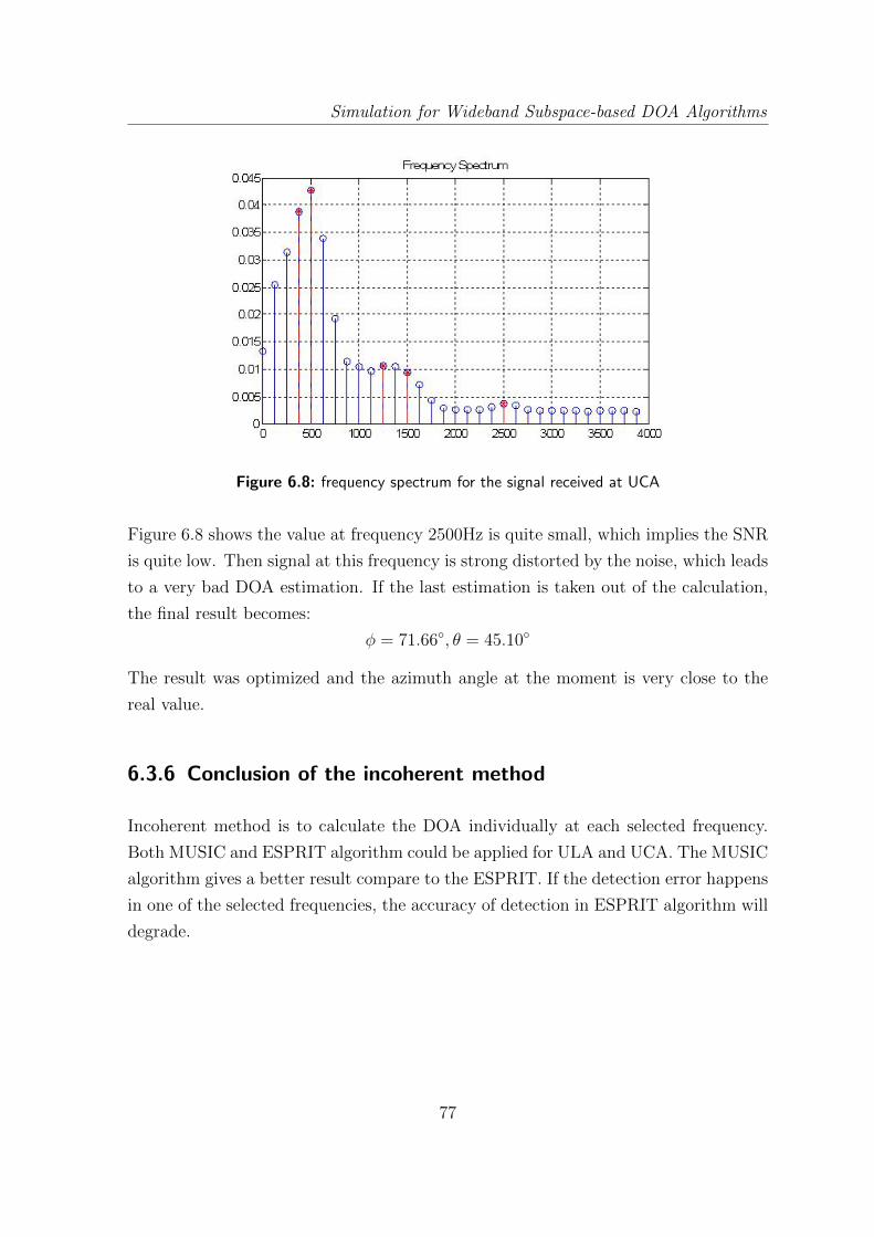
Simulation for Wideband Subspace-based DOA Algorithms
Figure 6.8: frequency spectrum for the signal received at UCA
Figure 6.8 shows the value at frequency 2500Hz is quite small, which implies the SNR
is quite low. Then signal at this frequency is strong distorted by the noise, which leads
to a very bad DOA estimation. If the last estimation is taken out of the calculation,
the final result becomes:
φ = 71.66◦, θ = 45.10◦
The result was optimized and the azimuth angle at the moment is very close to the
real value.
6.3.6 Conclusion of the incoherent method
Incoherent method is to calculate the DOA individually at each selected frequency.
Both MUSIC and ESPRIT algorithm could be applied for ULA and UCA. The MUSIC
algorithm gives a better result compare to the ESPRIT. If the detection error happens
in one of the selected frequencies, the accuracy of detection in ESPRIT algorithm will
degrade.
77
Simulation for Wideband Subspace-based DOA Algorithms
6.4 Coherent Wideband DOA Algorithms
The simulation for incoherent methods has been shown in the last section. Incoherent
method needs to calculate the narrowband DOA algorithms several times to get
either the spectrum or the DOA at each selected frequency, which depends on
which algorithm is used. The MUSIC algorithm needs to calculate the spectrum
for all detectable angle range, which is very time consuming but give a better
result. The ESPRIT is a close-form algorithm that give the DOA directly, but one
wrong result at one frequency will reduce the correctness of the final DOA estima-
tion. Therefore, the coherent method comes out which could reduce the computation
complexity and the result is obtain by only applying the narrowband method one time.
6.4.1 coherent signal subspace method (CSSM)
In last chapter, the concept of the coherent signal subspace method (CSSM) is in-
troduced. The core of the algorithm is to form the focusing matrices that transform
the steering vector from one frequency to the reference frequency. After focusing all
the steering vector, one covariance matrix at the reference frequency could be formed
by simply summing up the transformed covariance matrix. Then the narrowband al-
gorithm could be used to calculate the DOA by the covariance matrix at reference
frequency.
CSSM using MUSIC Algorithm in ULA
In ULA, the steering vector is a vector that contains the phase difference between
signal received at the N th microphone to the reference one.
a(θ) = [1, e−j2πfd sin(θ)/v, . . . , e−j2πf(N−1)d sin(θ)/v]
The value of steering vector depends on both the frequency and angle. Assuming the
angle is initialized, then the vector is only depending on the frequency. Let define the
following parameters:
78

Simulation for Wideband Subspace-based DOA Algorithms
• θ0 = 45◦, initialized DOA estimation
• fr = 1000Hz, reference frequency
• fi = 500Hz, signal frequency
The focusing matrix Ti is calculated by the following formulas:
Ti = ViUHi
Ui and Vi are respectively the right and left singular matrices of
A(fr, θf )AH(fi, θf )
And the calculated focusing matrix should be solve the following minimization prob-
lem:
minTi‖A(fr, θr)− TiA(fi, θr)‖
Initialized angle: θ0 = 45◦
A(fi, θr) A(fr, θr) TiA(fi, θr)1.0000 1.0000 1.0000
0.9578− 0.2873i 0.8349− 0.5504i 0.8349− 0.5504i
0.8349− 0.5504i 0.3940− 0.9191i 0.3940− 0.9191i
0.6415− 0.7671i −0.1769− 0.9842i −0.1769− 0.9842i
0.3940− 0.9191i −0.6895− 0.7243i −0.6895− 0.7243i
0.1133− 0.9936i −0.9743− 0.2252i −0.9743− 0.2252i
−0.1769− 0.9842i −0.9374 + 0.3483i −0.9374 + 0.3483i
−0.4523− 0.8919i −0.5909 + 0.8067i −0.5909 + 0.8067i
Table 6.3: Focusing matrix for MUSIC in ULA
Table 6.3 proves that the focusing matrix Ti realizes the minimization problem above.
In fact, the steering vector after focusing is the exactly the same as the one at the
reference frequency. Then the focusing matrix for the other frequencies could be
obtained by repeating the same steps. Then the covariance matrices after focusing
to the reference frequency need to be summed up to form a synthesized covariance
79

Simulation for Wideband Subspace-based DOA Algorithms
matrix.
Rcom =ku∑i=kl
αiTiRiTHi
The synthesized covariance matrix could be applied for the MUSIC algorithm.
The DOA angle could be calculated via the same steps in the narrowband MUSIC
algorithm.
Figure 6.9: coherent MUSIC algorithm with initial angle θ0 = 45◦
Figure 6.9 shows the spectrum that using the coherent method with initial angle 45◦.
The peak of the spectrum locates exactly at 45◦.
But the initial angle normally won’t be the same as the real DOA angle. The
wrong initial angle will form an imperfective focusing matrix, which leads an
imprecision detection result.
80

Simulation for Wideband Subspace-based DOA Algorithms
Figure 6.10: coherent MUSIC algorithm with initial angle θ0 = 30◦
Figure 6.10 shows the spectrum when the initial angle is changed to 30◦. The peak
in this case locates at 37◦. This tells the initial angle will decide the accuracy of the
detecting result. If the initial angle is not close to the real DOA, the detection result
by the coherent method is not reliable as well.
CSSM using ESPRIT algorithm in ULA
To form the focusing matrix for ESPRIT algorithm, the focusing matrices for each
subarray should be calculated at first. Then these two focusing matrices is combined
into one matrix.
θ0 θ45◦ 45.5163◦
30◦ 36.9162◦
60◦ 54.2659◦
Table 6.4: Coherent Signal Subspace Method using ESPRIT in ULA
81
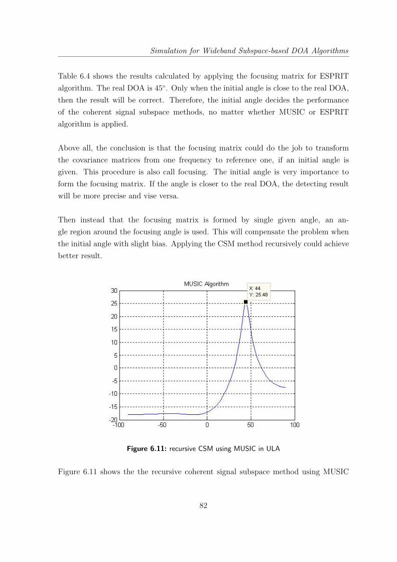
Simulation for Wideband Subspace-based DOA Algorithms
Table 6.4 shows the results calculated by applying the focusing matrix for ESPRIT
algorithm. The real DOA is 45◦. Only when the initial angle is close to the real DOA,
then the result will be correct. Therefore, the initial angle decides the performance
of the coherent signal subspace methods, no matter whether MUSIC or ESPRIT
algorithm is applied.
Above all, the conclusion is that the focusing matrix could do the job to transform
the covariance matrices from one frequency to reference one, if an initial angle is
given. This procedure is also call focusing. The initial angle is very importance to
form the focusing matrix. If the angle is closer to the real DOA, the detecting result
will be more precise and vise versa.
Then instead that the focusing matrix is formed by single given angle, an an-
gle region around the focusing angle is used. This will compensate the problem when
the initial angle with slight bias. Applying the CSM method recursively could achieve
better result.
Figure 6.11: recursive CSM using MUSIC in ULA
Figure 6.11 shows the the recursive coherent signal subspace method using MUSIC
82

Simulation for Wideband Subspace-based DOA Algorithms
algorithm. The initial angle is 30◦. The focusing range is from 10◦ to 50◦ at first.
After repeat the CSM three times, the peaks locates at 44◦, which is very close to the
real DOA.
Initialized angle: θ0 = 30◦
1st 2nd 3rd 4th 5th
36.9162◦ 40.0349◦ 44.0180◦ 45.0760◦ 45.0572◦
Table 6.5: recursive CSM using ESPRIT in ULA
It is also the same for doing recursive coherent signal subspace method using ESPRIT
algorithm. Table 6.5 shows the results when the initial angle is 30◦. After each
calculation, the resulting DOA angle is closer to the real DOA. In the end, a very
accurate result is obtained.
6.4.2 Robust Coherent Signal Subspace Method
The recursive CSM algorithm allows only certain amount bias for the initial angle.
When the angle is out of this range, the DOA detection will fail again. Therefore,
robust coherent signal subspace method (R-CSM) is developed. The big difference
between normal CSM method and R-CSM is that no initial angle is needed for
R-CSM. In ULA, the detectable angle range is from −89◦ to 90◦. Similar as the
recursive CSM that the focusing matrix is developed based on a given angle range,
the difference is that for R-CSM the very first focusing matrix is formed upon all
the detectable angle range. Applying this focusing matrix to get the synthesized
covariance matrix at reference frequency, the initial angle could be computed by
either MUSIC or ESPRIT algorithm. And afterwards, reduce the focusing range
around focusing angle and repeat the CSM methods until the result is getting stable.
83
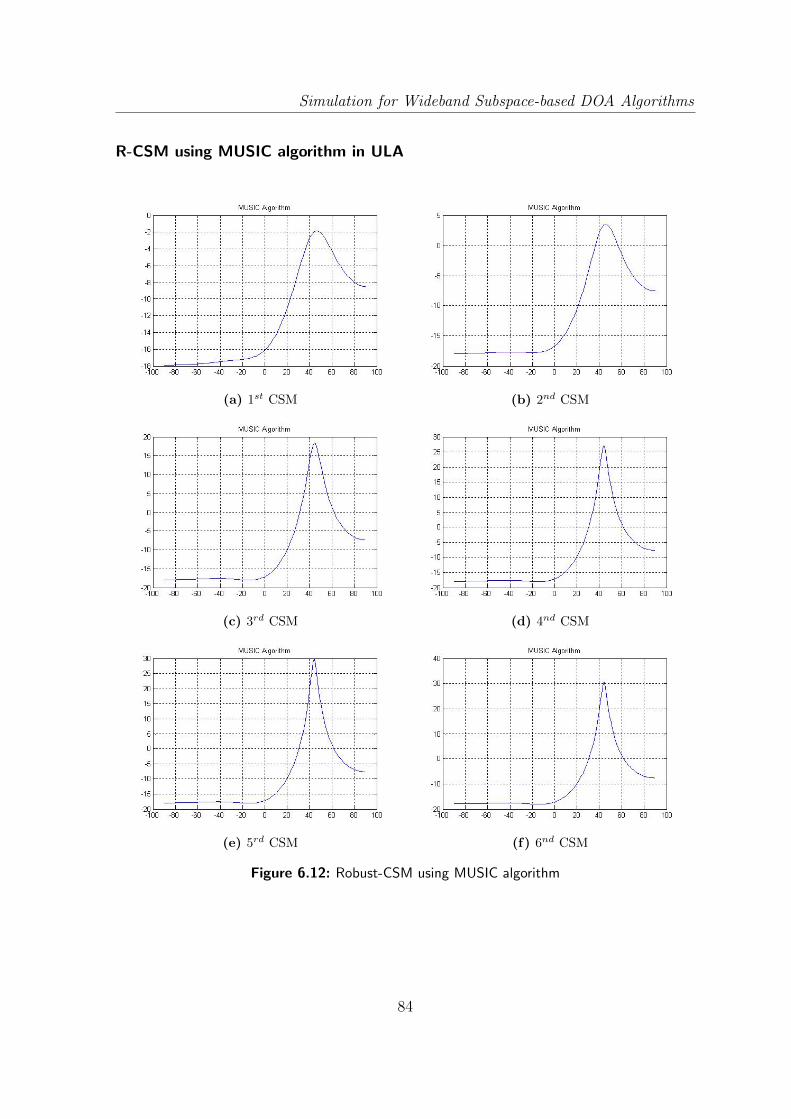
Simulation for Wideband Subspace-based DOA Algorithms
R-CSM using MUSIC algorithm in ULA
(a) 1st CSM (b) 2nd CSM
(c) 3rd CSM (d) 4nd CSM
(e) 5rd CSM (f) 6nd CSM
Figure 6.12: Robust-CSM using MUSIC algorithm
84
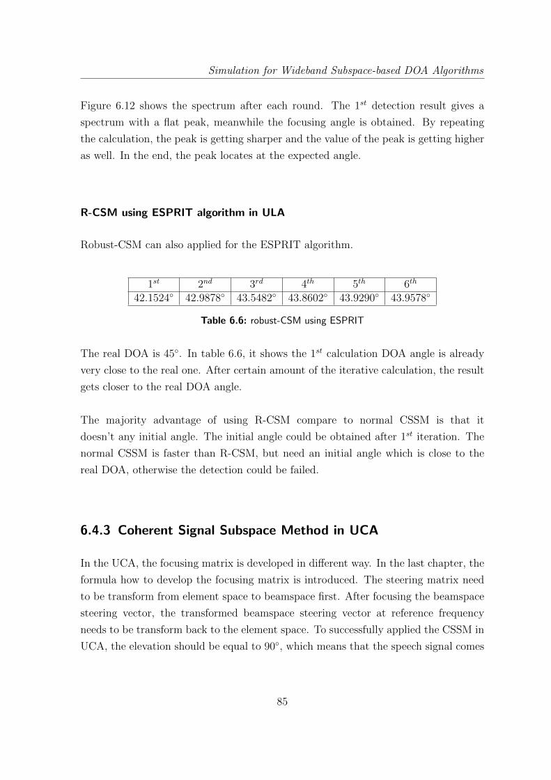
Simulation for Wideband Subspace-based DOA Algorithms
Figure 6.12 shows the spectrum after each round. The 1st detection result gives a
spectrum with a flat peak, meanwhile the focusing angle is obtained. By repeating
the calculation, the peak is getting sharper and the value of the peak is getting higher
as well. In the end, the peak locates at the expected angle.
R-CSM using ESPRIT algorithm in ULA
Robust-CSM can also applied for the ESPRIT algorithm.
1st 2nd 3rd 4th 5th 6th
42.1524◦ 42.9878◦ 43.5482◦ 43.8602◦ 43.9290◦ 43.9578◦
Table 6.6: robust-CSM using ESPRIT
The real DOA is 45◦. In table 6.6, it shows the 1st calculation DOA angle is already
very close to the real one. After certain amount of the iterative calculation, the result
gets closer to the real DOA angle.
The majority advantage of using R-CSM compare to normal CSSM is that it
doesn’t any initial angle. The initial angle could be obtained after 1st iteration. The
normal CSSM is faster than R-CSM, but need an initial angle which is close to the
real DOA, otherwise the detection could be failed.
6.4.3 Coherent Signal Subspace Method in UCA
In the UCA, the focusing matrix is developed in different way. In the last chapter, the
formula how to develop the focusing matrix is introduced. The steering matrix need
to be transform from element space to beamspace first. After focusing the beamspace
steering vector, the transformed beamspace steering vector at reference frequency
needs to be transform back to the element space. To successfully applied the CSSM in
UCA, the elevation should be equal to 90◦, which means that the speech signal comes
85

Simulation for Wideband Subspace-based DOA Algorithms
from quite far away.
The element-space steering vector in UCA is:
ϕm = kr sin θ cos(φ− 2πn− 1
N), where k =
2π
λ
After applying the phase mode excitation, the element-space steering vector is trans-
formed into beamspace:
f cm(θ) =1
N
N−1∑n=0
ejmγnejζcos(φ−γn) = jmJm(ζ)ejmφ
To prove that the focusing matrix works fine for both element-space and beamspace,
some initializations are made as followings:
• φ = 120◦, azimuth angle
• θ = 90◦, elevation angle
• fj = 500, signal frequency need to be focused
• fr = 1000, reference frequency
• N = 8, number of microphone
• M = 3, maximum phase mode
The focusing matrix is formed via the equation:
Ti = F−1BmF
where Bm = Jm(ζ0)/Jm(ζ)
86
Simulation for Wideband Subspace-based DOA Algorithms
A(fi) A(fr) TiA(fi)0.9788− 0.2046i 0.9163− 0.4006i 0.9174− 0.4005i
0.9943 + 0.1065i 0.9773 + 0.2117i 0.9762 + 0.2116i
0.9370 + 0.3494i 0.7558 + 0.6548i 0.7570 + 0.6549i
0.9218 + 0.3877i 0.6994 + 0.7147i 0.6982 + 0.7147i
0.9788 + 0.2046i 0.9163 + 0.4006i 0.9174 + 0.4005i
0.9943− 0.1065i 0.9773− 0.2117i 0.9762− 0.2116i
0.9370− 0.3494i 0.7558− 0.6548i 0.7570− 0.6549i
0.9218− 0.3877i 0.6994− 0.7147i 0.6982− 0.7147i
Table 6.7: Focusing matrix for UCA
Table 6.7 shows the steering vector before focusing after focusing. The steering vector
after focusing is very close to the one before focusing. Therefore, the focusing matrix
could transform the steering vector from 500Hz to 1000Hz with slight change.
TiA(fi)− A(fr) =
−0.0012− 0.0001i
0.0012 + 0.0001i
−0.0011− 0.0001i
0.0012 + 0.0000i
−0.0012 + 0.0001i
0.0012− 0.0001i
−0.0011 + 0.0001i
0.0012− 0.0000i
This bias is caused by transformation between element space and beamspace. The
inverse of the beamformer multiplying itself doesn’t give an identity matrix. The
error varies when the reference frequency or the azimuth angle changes. Compare
to the steering vector at the reference frequency, the error is quite small. Therefore,
these bias could be ignored. Then the focusing matrices for all the frequency need to
be calculated and focusing all the covariance matrices to the reference frequency. The
narrowband DOA algorithm, (UCA-RB-MUSIC or UCA-ESPRIT) could be applied.
To prove the correctness of the focusing matrix, an artificial array output is
created by the VPDs. Then the results before and after focusing are compared. The
algorithm applied here is UCA-ESPRIT.
87
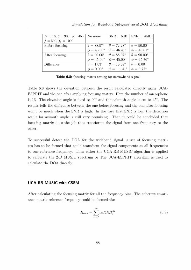
Simulation for Wideband Subspace-based DOA Algorithms
N = 16, θ = 90◦, φ = 45◦ No noise SNR = 5dB SNR = 20dB
f = 500, fr = 1000
Before focusing θ = 88.97◦ θ = 72.28◦ θ = 90.00◦
φ = 45.00◦ φ = 46.41◦ φ = 45.01◦
After focusing θ = 90.00◦ θ = 88.97◦ θ = 90.00◦
φ = 45.00◦ φ = 45.00◦ φ = 45.76◦
Difference θ = 1.03◦ θ = 16.69◦ θ = 0.00◦
φ = 0.00◦ φ = −1.41◦ φ = 0.77◦
Table 6.8: focusing matrix testing for narrowband signal
Table 6.8 shows the deviation between the result calculated directly using UCA-
ESPRIT and the one after applying focusing matrix. Here the number of microphone
is 16. The elevation angle is fixed to 90◦ and the azimuth angle is set to 45◦. The
results tells the difference between the one before focusing and the one after focusing
won’t be much when the SNR is high. In the case that SNR is low, the detection
result for azimuth angle is still very promising. Then it could be concluded that
focusing matrix does the job that transforms the signal from one frequency to the
other.
To successful detect the DOA for the wideband signal, a set of focusing matri-
ces has to be formed that could transform the signal components at all frequencies
to one reference frequency. Then either the UCA-RB-MUSIC algorithm is applied
to calculate the 2-D MUSIC spectrum or The UCA-ESPRIT algorithm is used to
calculate the DOA directly.
UCA-RB-MUSIC with CSSM
After calculating the focusing matrix for all the frequency bins. The coherent covari-
ance matrix reference frequency could be formed via:
Rcom =ku∑i=kl
αiTiRiTHi (6.3)
88

Simulation for Wideband Subspace-based DOA Algorithms
The approach is the same as what has been explained for the coherent wideband
DOA detection in ULA. Then UCA-RB-MUSIC could be applied to calculate the 2-D
MUSIC spectrum at the reference frequency. The corresponding azimuth and elevation
where the peak locates will be the expected DOA.
Figure 6.13: contour plot for coherent UCA-RB-MUSIC
Figure 6.13 shows the contour plot of the UCA-RB-MUSIC spectrum when the signal
source locates at θ = 90◦ and φ = 45◦. The signal-to-noise ratio is equal to 20dB. The
peak of the calculated spectrum locates at the position where θ = 78◦ and φ = 45◦,
which gives a correct azimuthal detection result. The result of the elevation angle is
imprecise. Here, the array consists of 16 microphones. The number of microphone is
not big enough to give a precise detection result for the elevation angle. More tests
will be proceeded in the UCA-ESPRIT.
UCA-ESPRIT with CSSM
As introduced before, the UCA-RB-MUSIC is not suitable to be applied for the hard-
ware implementation. The UCA-RB-MUSIC needs to calculate the spectrum at all
89

Simulation for Wideband Subspace-based DOA Algorithms
possible angle range. In addition, a 2D peak search has to be developed to find the
position of the peaks. Both of them cause the slowness of the algorithm. Therefore,
using the close-form algorithm UCA-ESPRIT is preferable. Normally the performance
of the algorithm is depending on the following parameters:
• azimuth angle(θ)
• elevation angles (φ)
• signal-to-noise ratio (SNR)
• number of the microphone (N)
Since the coherent signal subspace method is developed in the case that elevation is
equal to 90◦, therefore the elevation angle is keeping fixed and equal to 90◦.
SNR = 20dB,φ = 45◦ N = 8 N = 16 N = 32calculated result θ = 66.35◦ θ = 71.47◦ θ = 78.41◦
φ = 44.48◦ φ = 44.47◦ φ = 45.06◦
deviation θ = −23.65◦ θ = −18.53◦ θ = −11.58◦
φ = −0.52◦ φ = −0.5254◦ φ = 0.06◦
Table 6.9: coherent wideband UCA-ESPRIT 1
Table 6.9 shows the simulation results using UCA-ESPRIT with different number of
microphones. The deviation shows the difference between the calculated result and
expected angle. With the increment of the number of microphone, the elevation angle
is getting closer to the expected value. The azimuth angle doesn’t change much when
the number of microphone increases.
N = 16,φ = 45◦ SNR = 5dB SNR = 20dB no noisecalculated result θ = 90.00◦ θ = 71.47◦ θ = 72.78◦
φ = 44.02◦ φ = 44.47◦ φ = 45.00◦
deviation θ = 0.00◦ θ = −18.53◦ θ = −17.22◦
φ = −0.98◦ φ = −0.5254◦ φ = 0.00◦
Table 6.10: coherent wideband UCA-ESPRIT 2
90

Simulation for Wideband Subspace-based DOA Algorithms
Table 6.10 shows the simulation results using UCA-ESPRIT with different signal-
to-noise ratio. The signal source locates at the fixed direction. The number of
microphone is set to 16. When the noise is white sense, the detection result for the
azimuth angle is still promising even in the case that SNR is low. The accuracy of
the elevation result is not good.
N = 16, SNR = 20dB φ = −60◦ φ = 45◦ φ = 120◦ φ = −140◦
calculated result θ = 77.24◦ θ = 71.47◦ θ = 79.33◦ θ = 82.36◦
φ = −58.71◦ φ = 44.47◦ φ = 120.12◦ φ = −140.11◦
deviation θ = −12.76◦ θ = −18.53◦ θ = −10.67◦ θ = −7.64◦
φ = 1.29◦ φ = −0.5254◦ φ = 0.12◦ φ = −0.11◦
Table 6.11: coherent wideband UCA-ESPRIT 3
Table 6.11 shows the results when the source locates at different directions. The
result of the azimuth angle is of little deviation. These azimuth angles are taken
from each quadrant, which proves that the algorithm could detect the 360◦ azimuthal
angle. The elevation angle is comparable not as precise as the azimuth.
Above all, the tests have been made to check the performance of the coherent
wideband UCA-ESPRIT algorithm by varying the number of microphones, signal-to-
noise ratio and azimuth angle. The results shows the accurate azimuthal detection
requires not much hardware demanding. On the contrary, the accuracy of the el-
evation angle detection is not good even when a high number of microphone is applied.
For the project, the main goal is detecting the azimuthal angle correctly. The
elevation angle detection is an alternative. Therefore, the imprecision of the elevation
detecting result could be neglectable. In the next chapter, the real-time system will be
implemented which is based on this coherent wideband UCA-ESPRIT algorithm.
91
Chapter 7Real-time Implementation
In the previous chapter, the simulation has been presented for calculating DOA when
the signal is wideband. The coherent method gives a faster calculation if the ESPRIT
algorithm is chosen. The final goal of the project is to design a system that could
detect 360◦ azimuth angle range. Therefore, the UCA-ESPRIT will be chosen to be
implemented for the real-time system.
This chapter consists of the following parts. At first, the hardware settings are
going to be introduced. Then the steps for the implementation will be explained. In
the end, the test results will be analyzed and the performance of the system will be
discussed.
92

Real-time Implementation
7.1 Hardware Settings
7.1.1 DSK6713 + PCM3003
The board used for the real-time implementation is DSK6713 with the daughter board
PCM3003. The PCM3003 is an eight channel 16-bit audio codec daughter board,
suitable for the D.Module Family of DSP Computer Modules. The eight A/D and
D/A converters are sampled synchronously. The PCM3003 Delta-Sigma converters
provide excellent dynamic characteristics and inherent anti-aliasing and reconstruction
filtering.
Figure 7.1: DSK6713 + PCM3003
Figure 7.1 shows the TI-board DSK6713 with the daughter board PCM3003. More
details about the board could be found in the Master thesis of Mr. Saxena [6].
7.1.2 Uniform Circular Array
To implement UCA-ESPRIT algorithm, a uniform circular array is made which con-
tains eight microphones. Each microphone is connected with a pre-amplifier. The
93
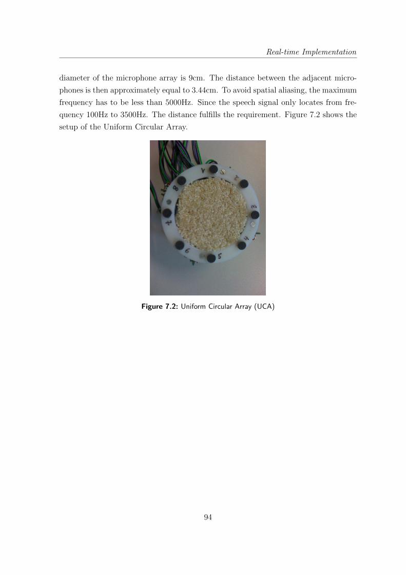
Real-time Implementation
diameter of the microphone array is 9cm. The distance between the adjacent micro-
phones is then approximately equal to 3.44cm. To avoid spatial aliasing, the maximum
frequency has to be less than 5000Hz. Since the speech signal only locates from fre-
quency 100Hz to 3500Hz. The distance fulfills the requirement. Figure 7.2 shows the
setup of the Uniform Circular Array.
Figure 7.2: Uniform Circular Array (UCA)
94

Real-time Implementation
7.2 Implementation of the algorithm
In the previous chapter, the basic concept of the UCA-ESPRIT has been introduced.
To successfully develop the coherent UCA-ESPRIT in real time, the following steps
shown in the following flow chart have to be implemented.
Figure 7.3: real time implement of UCA-ESPRIT algorithm
95

Real-time Implementation
7.2.1 Ping-Pong Buffering
The Ping-Pong Buffering is to use two buffers to store the sample date continuously
to avoid the situation that the data in the buffer changes during the processing.
While the EDMA is transferring the data into the Ping buffer, the CPU does the
processing in Pong buffer.
The interrupt routine edma complete int(void) is to check which EDMA buffer
is completed. When the flag block is equal to 0, it means the Ping buffer is complete.
When the flag block is equal to 1, it means the Pong buffer is complete. In the
program, it is only necessary to check whether a new block is complete. Therefore,
the flag block is initialized to -1 after each calculation. A while loop is created to wait
until the value of the flag changes.
7.2.2 Distinguishing between noise and signal
After the buffer is full, the main program starts. But it doesn’t know at first whether
the data stored in the buffer is the speech signal or just the noise. There is no sense to
proceed the algorithm when only the silence signal was taped. To distinguish the data
in the buffer whether is speech or noise, the power of signal was calculated. A threshold
is defined in preliminary. When the power exceed the threshold, it is assumed that
the input data is speech signal and the algorithm could be proceeded. Otherwise, the
program has to wait until the next buffer is full.
7.2.3 Amplitude calibration
In the simulation, the VPDs method creates the artificial signals for the array
output. The signals received at microphones are assumed to be identical. However in
reality, the microphone normally has difference sensitivity, which causes the different
attenuation factors. Therefore the signal arrived at each microphone has to be
calibrated in the beginning.
96

Real-time Implementation
Here a very simple method is developed to realize the gain calibration. The
power of the sampled speech signal at each microphone is calculated at first. Then
gain ratio is obtained by calculating the square root of the ratio between the powers
of N th microphone and the 1st one. When the gain ratio is calculate, the calibrated
signal will be obtained by
xi = αixi
where αi is the gain ratio between the N th microphone and the 1st one.
7.2.4 Fast Fourier Transform
Before selecting the fundamental frequencies, the spectrum of the input signal has to
be calculated. The FFT algorithm used in the program is from TMS320C6713 DSP
library [17]. It consists of following functions:
gen w r2(W, BUFLEN);
bit rev(W, BUFLEN � 1);
cfftr2 dit(x fft, W, BUFLEN);
bit rev(x fft, BUFLEN);
To save the calculation load, the twiddle factor W needs to be calculated once before
the main program and pass to the function as a parameter.
7.2.5 Adaptive selection of fundamental frequencies
After the complex value spectrum is calculated, the power spectrum could be obtained
by simply sum up the square value of the real and imaginary parts. The whole fre-
quency range could be separated into several bins. Then the fundamental frequencies
could be obtained by searching the peak values in each bin. Then all the peak val-
ues will be sorted descendingly. The corresponding frequencies with the highest peak
values will be the selected fundamental frequencies.
97

Real-time Implementation
7.2.6 Coherent Covariance Matrix
Now the fundamental frequencies have been calculated. The covariance matrices at
the selected frequency could be formed.
Ri = XiXHi ;
As introduced in the previous chapter, the focusing matrix is used to translate the
steering vector from one frequency to the reference one. Here the focusing matrices
for all the frequencies have been pre-calculated. Then the coherent covariance matrix
could be calculated via
Rcom =K∑i=1
TiRiTHi ;
7.2.7 Element-space to Beam-space
When the coherent covariance is formed, then the classic UCA-ESPRIT could be
applied for detecting the DOAs. The first step of UCA-ESPRIT is to transform
the covariance from element-space to beamspace by using beamforming matrix. The
beamforming matrix is determined by the maximum phase mode (M) and number of
microphones (N). Therefore, the beamforming matrix could be pre-calculated to save
computation load. In the introduction of the UCA-ESPRIT, it has been shown that
the algorithm only needs the real-part of the covariance matrix. Then the function
elementToBeamspace(Rcom, cov fmatrix) is made to realized the followings:
FHr RcomFr;
The result will be the beamspace covariance matrix at the reference frequency.
7.2.8 Singular Value Decomposition
After transforming the coherent covariance matrix from element space to beamspace,
the matrix has to be applied for a decomposition function to extract the signal
subspaces. As introduced in the theory, the UCA-ESPRIT only requires a real-value
98

Real-time Implementation
decomposition. Unlike the complex value decomposition applied for MUSIC and
ESPRIT in ULA, the real-value decomposition makes the real-time system faster.
The method is already implemented by Mrs Bing Li and Mrs Yuan Cheng in
their thesis [16]. The function called is
svdcmp(cov matrix real,2*M+1,2*M+1,svd u,svd v)
After transformation, the beamspace covariance matrix has the dimension (2M+1)×(2M + 1), where M is the maximum phase mode. Therefore, the dimension of the
column vector svd u is equal to the one of the row vector svd v, which is equal to
(2M + 1). And the first row of the column vector is the beamspace signal subspace.
7.2.9 Calculation of the DOAs
Then according to the introduction of the UCA-ESPRIT algorithm, the signal sub-
space vector needs to be separated into three sub-vectors at first. Afterwards, three
block matrices B, C, Q are formed via:
B = SH−1S−1
C = SH−1DIS∗−1
Q = SH−1ΓS0
The corresponding methods that are created to realized these equations are the fol-
lowings:
B = B cal(S Minus);
C = C cal(S Minus,S Plus);
Q = Q cal(S Minus,S Zero,freq);
99
Real-time Implementation
The complex value Ψ could be obtained via the function
Psi = Psi cal(B,C,Q);
The calculated complex value Ψ contains the information of both the elevation and
azimuth angles.
θ = sin(−1)(√
ΨRΨR + ΨIΨI)
φ = tan−1(ΨI/ΨM)
When the azimuth is calculated, the quadrant could be determined by the sign of the
real and image parts of the Ψ. When the magnitude of the Ψ is larger than 1, it is
not possible to calculate the arcsin value. In this case, the elevation angle is simply
assigned to 90◦.
7.3 Testing Results
Two real-time systems are set up. One is to detect the narrowband signal, which the
signal source is a sinusoidal wave with certain frequency. In the narrowband real-time
system, there is no need to select certain amount of fundamental frequencies, because
the sinusoidal wave only contains only one frequency component. In addition, in
stead of doing classic DOA detect at reference frequency after focusing the covariance
matrix, the narrowband real-time system is directly applied for the covariance matrix
at the fundamental frequency.
The other real-time system is implemented based on the coherent wideband
UCA-ESPRIT algorithm. Here certain number of the frequency components that
have the higher magnitudes are selected. The covariance matrices on these frequencies
are translated into the reference frequency by using focusing matrix. The narrowband
UCA-ESPRIT algorithm then calculate the DOA with the covariance matrix at
reference frequency. The normal speech signal or a piece of music sound could be
used as the signal source.
100

Real-time Implementation
7.3.1 Testing Environment
Both the narrowband testing and wideband testing are done in a lab room. The signal
is corrupted by the noise such as the PC sound, air-condition, and the reverberation
signals. To successfully applied the UCA-ESPRIT algorithm, the noise is assumed to
be white. In the reality, it is always not realistic.
Figure 7.4: Spectrum of the noise in the lab room
Figure 7.4 shows the spectrum of the signal received at 1st microphone when there
is no signal source applied. It is obvious to notice that the noise is not white here.
There is one 50Hz frequency component which caused by the power supply. The other
frequencies components are comparatively very low, which could be neglectable. For
the fundamental frequency selection in the algorithm, the frequency will be selected
between the range 100Hz and 3500Hz. Therefore, the frequency component below
100Hz won’t be taken into consideration. In another word, the 50Hz power line noise
won’t affect the detecting result.
7.3.2 Testing Results for Narrowband Signals
The sinusoidal signals with different frequencies are applied to test the accuracy of the
narrowband real-time system. The test result is shown in the followings.
101
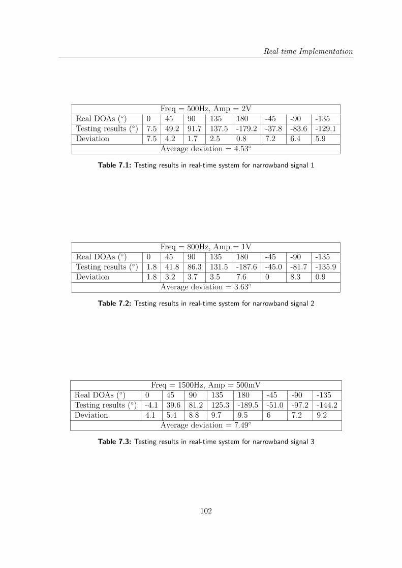
Real-time Implementation
Freq = 500Hz, Amp = 2VReal DOAs (◦) 0 45 90 135 180 -45 -90 -135Testing results (◦) 7.5 49.2 91.7 137.5 -179.2 -37.8 -83.6 -129.1Deviation 7.5 4.2 1.7 2.5 0.8 7.2 6.4 5.9
Average deviation = 4.53◦
Table 7.1: Testing results in real-time system for narrowband signal 1
Freq = 800Hz, Amp = 1VReal DOAs (◦) 0 45 90 135 180 -45 -90 -135Testing results (◦) 1.8 41.8 86.3 131.5 -187.6 -45.0 -81.7 -135.9Deviation 1.8 3.2 3.7 3.5 7.6 0 8.3 0.9
Average deviation = 3.63◦
Table 7.2: Testing results in real-time system for narrowband signal 2
Freq = 1500Hz, Amp = 500mVReal DOAs (◦) 0 45 90 135 180 -45 -90 -135Testing results (◦) -4.1 39.6 81.2 125.3 -189.5 -51.0 -97.2 -144.2Deviation 4.1 5.4 8.8 9.7 9.5 6 7.2 9.2
Average deviation = 7.49◦
Table 7.3: Testing results in real-time system for narrowband signal 3
102

Real-time Implementation
Table 7.1 - 7.3 show the testing results for detecting the sinusoidal signal with f1 =
500Hz, f2 = 800Hz, f3 = 500Hz. The deviations have slight change when the signal
frequency changes. The error between the calculate results and real DOA angle is
smaller than 10◦. This proves the UCA-ESPRIT could localize the speaker with small
error. The initial DOA angles are chosen from four quadrants, which covers 360◦
azimuthal angle. This tells that the UCA-ESPRIT can detect the angle from all
azimuthal direction.
7.3.3 Testing Results for Normal Speech
The coherent UCA-ESPRIT algorithm is implemented for localizing the wideband
signal source. To test the performance of the real-time application, the speaker speaks
from different directions to see the correctness of the result.
Real DOA Testing results Deviation135 132 134 135 137 134 1.3
90.0 92.5 82.9 88.3 89.9 88.7 2.545.0 42.9 47.2 52.4 41.6 46.6 3.30.0 -5.2 -11.2 -11.0 -6.6 -2.2 7.2
-45.0 -37.7 -34.8 -41.8 -40.8 -39.4 6.1-90.0 -88.4 -91.1 -84.5 -91.3 -80.2 3.9
-135.0 -135.9 -130.5 -140.6 -133.8 -141.4 3.7-180.0 -177.1 168.5 -171.6 -177.0 169.1 7.4
Table 7.4: Testing results in real-time system for normal speech signal
Table 7.4 shows the testing results of the coherent UCA-ESPRIT algorithm when
normal speech is applied. The standard deviation between the testing results and the
real DOAs are with 10◦. The average value of the standard deviations is 4.4◦. This
proves the coherent UCA-ESPRIT works properly for the real-time.
103

Chapter 8Conclusion and Future works
In this thesis, a DSP-based DOA detecting real-time system is implemented, which
could correctly detect the 360◦ azimuthal angle. The UCA-ESPRIT algorithm which
is developed on the Uniform Circular Array is the basic algorithm behind the system.
The classic DOA algorithm such as MUSIC, ESPRIT in the ULA can only de-
tect the azimuth angle from −90◦ to 90◦. MUSIC requires calculate the MUSIC
spectrum for all the possible azimuthal angle and a peak search algorithm has to be
implemented afterwards to find direction-of-arrival angle. Unlike MUSIC, ESPRIT
is close-form DOA algorithm which doesn’t need an expensive spectral search. But
ESPRIT requires two identical subarrays. The mismatch between the subarrays leads
to the error of the detecting results.
Similar as ULA, there are also two DOA algorithms (UCA-RB-MUSIC and
UCA-ESPRIT) in UCA. Both algorithms need to transform the element-space
steering vector into beamspace via phase mode excitation. Then the beamspace
steering vector becomes Vandermonde-like structure. The UCA-RB-MUSIC is to
calculate the MUSIC spectrum in beamspace. UCA-ESPRIT is using the properties
of the Bessel function to extract the angle directly. The phase mode excitation
reduces the length of the element and only the real-part of the beamspace covariance
matrix is taken into calculation. These factors make the speed of the UCA-ESPRIT
faster.
104

Conclusion and Future works
The classic UCA-ESPRIT can only detect the DOA of the narrowband signals.
To successfully localize the speaker, the wideband DOA algorithm has to be imple-
mented. Here, a coherent wideband DOA algorithm is created. Unlike incoherent
method, coherent method requires to calculate the narrowband DOA algorithm
only once. Only the assumption has to be fulfilled that the speaker has to be far
from the microphone array, which make the elevation angle approximately equal to 90◦.
The test is done in a noisy room. The results shows that the deviation for de-
tecting the narrowband signal sources is less than 10◦. The error for localize the
wideband signal (normal speech signal) is even less. Both show that the system could
have a good performance to detect azimuthal angle.
8.1 Improvement and Future work
In the real time, the signals arrived at each microphone are attenuated with different
levels. The system calculates the power of the sampled signal at each microphone to
get the gain ratio to realize the amplitude calibration. This approach is the easiest
but requires a lot resources to calculate, which slows down the system. To solve the
problem, a AGC (Automatic Again Control) application could be developed to replace.
In this project, the DSP-board could only tape eight channel simultaneously.
Therefore, the Uniform Circular Array is formed with only eight microphones. In the
future, the application could be realized on a UCA with more microphones, which
could improve the detecting results.
The detecting error is caused by a lot of reasons. Perhaps the noise in the
room is not white enough, which distorted the signal at the selected frequencies. Or
the microphone array is not well constructed. To solve these problems, an adaptive
filter could be applied to attenuate the noise and an array shape calibration could be
developed to compensate the imperfection of the UCA. Both of them require a lot
of the computation load and will affect the speed of the real time application. It is
105

Conclusion and Future works
always a trade-off between the speed and accuracy.
106
Bibliography
[1] R. A. Monzingo and T. W. Miller, Introduction to Adaptive Arrays. New York:
Wiley, 1980.
[2] S.U. Pillai. Array Signal Processing. Springer-Verlag, New York, 1989.
[3] S.S. Haykin. Array Signal Processing, chapter 4. S.S. Haykin Ed., Prentice- Hall,
New Jersey, 1985.
[4] R.O. Schmidt. Multiple emitter location and signal parameter estimation. IEEE
Trans. Antennas Propagat., 34(3):276-280, March 1986.
[5] R. Roy and T. Kailath. ESPRIT-Estimation of signal parameters via rota-
tional invariance techniques. IEEE Trans. Acoust., Speech, Signal Process-
ing, 37(7):984-995, July 1989. IEEE Trans. Antennas Propagat., 34(3):276-280,
March 1986.
[6] Master Thesis (Wideband Audio Source Localization using Microphone Array
and MUSIC Algorithm), Anshul Kant Saxena
[7] Diplomarbeit (DSP-basiertes Echtzeitsystem zur Sprecherlokalisierung mittels
Mikrofonarray und Root-MUSIC), Kolja Pikora
[8] Balanis, C. A., Antenna Theory: Analysis and Design, 3rd ed., New York: Wiley,
2005.
107

Bibliography
[9] J. Yang and M. Kaveh, Adaptive eigensubspace algorithms for direction or fre-
quency estimation and tracking, IEEE Transactions on Acoustics, Speech, Signal
Processing, vol. 36, pp. 241C251, Feb. 1988. doi:10.1109/29.1516
[10] H. Krim and M. Viberg, Two decades of array signal processing research: the
parametric approach, IEEE Signal Processing Magazine, vol. 13, pp. 67C94, July
1996. doi:10.1109/79.526899
[11] L. C. Godara, Application of antenna arrays to mobile communications. Part II:
Beamforming and direction of arrival considerations, Proceedings of the IEEE,
vol. 85, pp. 1195C 1245, Aug. 1997. doi:10.1109/5.622504
[12] T. S. Rappaport and J. C. Liberti Jr., Smart Antennas for Wireless Communi-
cations: IS-95 and Third Generation CDMA Applications, Upper Saddle River,
NJ: Prentice Hall, 1999.
[13] D. E. N. Davies, Circular arrays, Chap. 12, The Handbook of antenna design,
London Peregrinus on behalf of the IEE, 1983.
[14] D. E. N. Davies, A transformation between the phasing techniques required for
linear and circular aerial arrays, Proc. IEE, Vol. 112, No. 11, Nov 1965.
[15] C. P. Mathews, M. D. Zoltowski, Eigenstructure techniques for 2-D angle esti-
mation with uniform circular arrays, IEEE Trans. Signal Proc., Vol. 42, No. 9,
Sept 1994, pp. 2395-2407.
[16] Master-Thesis (DSP-Based Acoustic Source Localization, Master-Thesis, 2004),
Mrs Bing Li and Mrs Yuan Cheng
[17] Texas Instruments, ”TMS320C67xDSP Library”, Programmer’s Reference
Guide, SPRU657B, March 2006
[18] Chandran, S., and M. K. Ibrahim, DOA Estimation of Wide-Band Signals Based
on Time-Frequency Analysis, IEEE J. of Oceanic Engineering, Vol. 24, No. 1,
January 1999, pp. 116C121.
[19] Wax, M., and T. Kailath, Spatio-Temporal Spectral Analysis by Eigen-Structure
Methods, IEEE Trans. on Acoustics, Speech, and Signal Processing, Vol. ASSP-
32, No. 4, August 1984, pp. 817C827.
108
Bibliography
[20] Wang, H., and M. Kaveh, Coherent Signal-Subspace Processing for the Detection
and Estimation of Angles of Arrival of Multiple Wide-Band Sources, IEEE Trans.
on Acoustics, Speech, and Signal Processing, Vol. ASSP-33, August 1985, pp.
823C831.
[21] Fabrizio Sellone, Robust auto-focusing wideband DOA estimation, Signal Pro-
cessing., vol.86, pp.17-37, .2006.
[22] PROF. DR. KOElZER and PROF. DR. SAUVAGERD, Digital Signal Process-
ing, chap. Efficient structures for Sample Rate Converters (SRCs)
109