TU WIEN

DIPLOMA THESIS

Robust CSI feedback for

high user velocity

Institute of Telecommunications of Vienna University of Technology

Laura Portolés Colón

11/18/2014

1

2

Abstract

The significant growth of mobile communications usage and the development of new

applications that require a wide information flow in the past few years have been the

primordial motivations in the investigation of the new mobile communications

standard, LTE (Long Term Evolution). Release 8 was concluded for the 3GPP (Third

Generation Partnership Project) in 2008. Significantly higher transmission rates than

with the previous technologies has been achieved, up to 326.5 Mbit/s in downlink and

up to 86.5 Mbit/s in uplink transmissions due to several improvements that have been

introduced on different parts of the communication system.

The work realised in this thesis consist of improving the communications in high

velocity scenarios where the channel characteristics deteriorate significantly by means

of weak temporal correlation between channel realizations and large latency in the

feedback reporting from the UE (User Equipment) to the base station (eNodeB). For

these reasons this thesis is performed with the downlink link level LTE simulator,

available at the Institute of Telecommunications of Vienna University of Technology.

The focus of the work is on estimating the feedback parameters, necessary for link

adaptation, in high velocity scenarios.

Previously, link adaptation has been optimized for scenarios at low velocity where zero

uplink delay can be assumed to obtain sufficiently accurate results. For that reason the

CSI (Channel State Information) calculation, which is performed in the receiver, is

based on instantaneous channel knowledge. As a result of the increasing velocity the

performance at the mobile user decreases drastically, because the CSI provided to the

base station and utilized for selection of the transmission parameters is very outdated,

due to a non-negligible delay in the feedback path. Specifically the CSI consist of three

feedback indicators, whose objective is maximizing all the possible gains that OFDM

(Orthogonal Frequency Division Multiplexing) and MIMO (Multiple-Input Multiple-

Output) offer, enhancing the channel efficiency while maintaining the BLER (Block Error

Ratio) below a certain bound, typically fixed to 10% in wireless communications. These

three indicators are, CQI (Channel Quality Indicator), RI (Rank Indicator) and PMI

(Precoding Matrix Indicator). At high velocity the estimation of these indicators is not

accurate enough whether their calculation is exclusively based on the current channel

information. Precisely for that reason in this thesis new feedback algorithms that take

into account the channel statistics are implemented.

The final objectives of these robust algorithms are the improvement of the channel

performance by means of increased throughput and reduced BLER measured in the

receiver.

3

Acknowledgements

I am very glad to have performed this thesis at the Institute of Telecommunications of

Vienna University of Technology. I would like to express my gratitude in first place to

Prof. Markus Rupp (Vienna University) to allow me to take part in the LTE research

group, and in second place to Stefan Schwarz (Vienna University) that has continuously

supervised my work leading me to find new solutions to develop in the LTE Vienna

simulator. Furthermore, I would like to thank Paloma Garcia (Zaragoza University) for

her suggestions and advice from Spain.

There are many other important people that have been present in my life during these

last months that I have spent in Vienna. Perhaps they were not with me personally,

however, from the distance they have always supported and encouraged me with my

studies. The most important are my parents, Inma and Santiago, my sister Cristina and

Jaime. Without their backup I could have never lived this unique experience.

4

Table of Contents

Abstract ......................................................................................................................................... 2

Acknowledgements ....................................................................................................................... 3

List of Figures ................................................................................................................................ 6

List of tables .................................................................................................................................. 7

List of abbreviations ...................................................................................................................... 8

1. INTRODUCTION AND MOTIVATION .................................................................................... 10

2. LONG TERM EVOLUTION ..................................................................................................... 14

2.1 Long Term Evolution description ................................................................................ 14

2.1.1 Mobile communications evolution ..................................................................... 14

2.1.2 LTE requirements and characteristics ................................................................. 15

2.1.3 Network architecture .......................................................................................... 16

2.1.4 Physical layer ....................................................................................................... 16

2.2 LTE feedback modelling............................................................................................... 19

2.2.1 User equipment feedback indicators .................................................................. 19

2.2.2 Transmission modes ............................................................................................ 21

2.2.3 SISO feedback calculation ................................................................................... 23

2.2.4 MIMO CSLM feedback calculation ...................................................................... 23

2.3 High velocity consequences ........................................................................................ 26

2.4 Vienna LTE simulators ................................................................................................. 29

2.4.1 Main simulation parameters ............................................................................... 30

3. FEEDBACK ALGORITHMS TO IMPROVE THE USER THROUGHPUT ...................................... 34

3.1 Study of the CQI .......................................................................................................... 34

3.1.1 SINR Long-term average ...................................................................................... 34

3.1.2 Maximum throughput expected ......................................................................... 35

3.1.3 Conditional CQI probability ................................................................................. 36

3.1.4 SINR variation ...................................................................................................... 37

3.1.5 Methods comparison and adaptation to different velocity ................................ 39

3.2 Study of the RI and PMI ............................................................................................... 42

3.2.1 Code modifications .............................................................................................. 43

3.2.2 Results ................................................................................................................. 44

3.3 Frequency-selective channel with multiple users ....................................................... 47

5

4. FEEDBACK ALGORITHMS TO ACHIEVE THE 0.1 BLER TARGET ............................................. 50

4.1 Study of the CQI .......................................................................................................... 50

4.1.1 0.1 BLER target method ...................................................................................... 50

4.1.2 BLER expected method ....................................................................................... 51

4.1.3 Methods comparison and evaluation over normalized Doppler frequency ....... 52

4.2 Study of the RI and PMI ............................................................................................... 54

4.2.1 CLSM Code modifications .................................................................................... 54

4.2.2 Results ................................................................................................................. 54

4.3 Frequency-selective channel with multiple users ....................................................... 56

5. CONCLUSIONS AND FUTURE RESEARCH ............................................................................. 60

References ................................................................................................................................... 62

6

List of Figures

Figure 2-1 3GPP Technology Evolution (referencia) ................................................................... 14

Figure 2-2 Network architecture -LTE/EPC Reference Architecture ........................................... 16

Figure 2-3 OFDM subcarrier spacing ........................................................................................... 17

Figure 2-4 LTE time-frequency grid structure (reference) .......................................................... 18

Figure 2-5 BICM capacity of 4, 16 and 64-QAM modulation [4] ................................................. 24

Figure 2-6 Temporal correlation in a Rayleigh fading channel ................................................... 27

Figure 2-7 SINR variation between consecutive subframes at high velocity .............................. 28

Figure 2-8 Performance loss due to the feedback delay............................................................. 28

Figure 2-9 Downlink link level simulator architecture ................................................................ 30

Figure 3-1Maximum throughput curves for CQI 1-15 ................................................................. 34

Figure 3-2 CQI dependant on the previous CQI .......................................................................... 37

Figure 3-3 T location-scale distribution function ........................................................................ 38

Figure 3-4 Throughput improvement methods comparison ...................................................... 39

Figure 3-5 SISO Throughput over normalized Doppler Frequency and beta = 10 ...................... 40

Figure 3-6 Throughput comparison with a linear predictor ........................................................ 41

Figure 3-7 BLER comparison with a linear predictor ................................................................... 42

Figure 3-8 2x2 MIMO, Zero antenna correlation ........................................................................ 44

Figure 3-9 2x2 SU-MIMO throughput with 0.5 receiver antenna correlation ............................ 45

Figure 3-10 2x2 SU-MIMO throughput improvement with 0.5 antenna correlation ................. 45

Figure 3-11 4x8 SU-MIMO throughput with 0.5 receiver antenna correlation and throughput

improvement ............................................................................................................................... 46

Figure 3-12 2x2 SU-MIMO throughput comparisons with the original feedback method ......... 46

Figure 3-13 4x8 SU-MIMO throughput comparisons with the original feedback method ......... 47

Figure 3-14 Cell throughput improvement using SINR long-term average method ................... 48

Figure 3-15 Cell BLER improvement using SINR long-term average method ............................. 49

Figure 4-1 BLER curves for CQI 1-15 with zero correlation and 10ms uplink delay .................... 51

Figure 4-2 BLER curves for CQI 1-15 with maximum correlation and zero uplink delay ............ 52

Figure 4-3 Methods comparison that achieve the 10% BLER ..................................................... 53

Figure 4-4 Methods comparison that achieve 10% BLER over �� .............................................. 53

Figure 4-5 2x2 MIMO, throughput improvement achieved using the BLER expected method .. 54

Figure 4-6 4x8 MIMO, throughput improvement achieved using the BLER expected method .. 55

Figure 4-7 2x2 MIMO, final results that achieve the BLER target ............................................... 56

Figure 4-8 4x8 MIMO, Final results that achieve the BLER target .............................................. 56

Figure 4-9 Cell throughput improvement with BLER expected method ..................................... 57

Figure 4-10 Cell BLER improvement with BLER expected method ............................................. 58

7

List of tables Table 2-1 OFDM configuration .................................................................................................... 17

Table 2-2 LTE codebook for CSLM mode and two transmit antennas ........................................ 20

Table 2-3 Modulation scheme and effective coding rate for each of the Channel Quality

Indicators (CQIs) .......................................................................................................................... 21

Table 2-4 Constant simulation parameters ................................................................................. 30

Table 2-5 Simulation parameters utilized do develop the methods to estimate the CQI .......... 31

Table 2-6 Simulation parameters utilized to compare the CQI methods over �� ...................... 31

Table 2-7 Simulation parameters in order to study PMI and RI.................................................. 31

Table 2-8 Simulation parameters to evaluate the methods in a frequency selective channel .. 32

8

List of abbreviations

3GPP Third Generation Partnership Project

AMC Adaptative Modulation and Coding

ARQ Automatic Repeat reQest

AWGN Additive White Gaussian Noise

BICM Bit Interleaved Code Modulation

BLER Block Error Ratio

CB Code Block

CC Chase Combining

CLSM Closed Loop Spatial Multiplexing

CP Cyclic Prefix

CQI Channel Quality Indicator

CRC Cyclic Redundancy Check

CSI Channel State Information

CW Codeword

EPC Evolved Packet Core

ERC Effective Code Rate

E-UTRAN Evolved Universal Terrestrial Radio Access Network

EWMA Exponentially Weighted Moving Average

FDD Frequency Division Duplex

FFT Fast Fourier Transform

GPRS General Packet Radio Services

GSM Global System for Mobile communications

HARQ Hybrid Automatic Repeat reQuest

HSPA High Speed Packet Access

ICI Inter Carrier Interference

IFFT Inverse Fast Fourier Transform

IMT International Mobile Telecommunications

IP Internet Protocol

IR Incremental Redundancy

ISI Inter Symbol Interference

ITU International Telecommunication Union

LMMSE Linear Minimum Mean Squared Error

LTE Long Term Evolution

LTE Long Term Evolution

LTE-A Long Term Evolution Advanced

MAC Medium Access Control

MCS Modulation and Code Schemes

MIESM Mutual Information Based Exponential SNR Mapping

9

MIMO Multiple-Input Multiple-Output

MME Mobility Management Entity

OFDMA Orthogonal Frequency Division Multiplexing Access

OLSM Open Loop Spatial Multiplexing

PAPR Peak-to-Average Power Ratio

PCCC Parallel Concatenated Convolutional Code

P-GW Packet data network Gateway

PHY Physical Layer

PMI Precoding Matrix Indicator

QAM Quadrature Amplitude Modulation

RB Resource Block

RE Resource Element

RI Rank Indicator

RLC Radio Link Control

RRM Radio Resource Management

SAE System Architecture Evolution

SC-FDMA Single Carrier Frequency Division Multiplexing Access

S-GW Serving Gateway

SINR Signal to Interference plus Noise Ratio

SISO Single-Input Single-Output

SNR Signal to Noise Ratio

SSD Soft Sphere Decoding

STBC Space-Time Block Code

TB Transport Block

TDMA Time Division Multiplexing Access

TTI Transmission Time Interval

TU Typical Urban

UE User Equipment

UMTS Universal Mobile Telecommunication System

WCDMA Wideband Code Division Multiplexing Access

ZF Zero Forcing

10

1. INTRODUCTION AND MOTIVATION

After about twenty years of practically uninterrupted growth of mobile

communications, not only referred to voice but also video streaming and other real

time applications that require wideband data flow, a new generation of wireless

communication, 3G, has been exhaustively investigated in the past few years. LTE

(Long Term Evolution), is a new standard, concluded for the 3GPP (Third Generation

Partnership Project) in 2008 (Release 8), which can be considered the first step in the

evolution that will culminate with LTE-Advanced (4G). The most relevant aspects

about LTE are that for the first time IP (Internet Protocol) is supported for all its

services, voice included, and the peak rates reached in the radio interface are in the

range of 100Mbit/s to 1Gbit/s, considerably higher than with previous technologies,

namely, GSM (Global System for Mobile communications) or UMTS (Universal Mobile

Communication System) Release 7. Furthermore it was expected that with the

appearance of LTE the capacity achieved by the mobile users would not be

substantially penalized because of the velocity, however this goal is not achieved.

The high transmission rates can be achieved by virtue of the new physical layer

architecture implemented, together with other improvements. OFDMA (Orthogonal

Frequency Division Multiplexing Access) modulation scheme is utilized in DL (Downlink)

transmissions whose advantage with respect to the previous modulation schemes used

is that it converts the wide-band frequency selective channel into a set of many flat

fading subchannels. The fact that the signal is divided into flat fading channels has

some advantages, for instance that optimum receivers can be implemented with

reasonable complexity in contrast to WCDMA (Wideband Code Division Multiplexing

Access) utilized in the previous communication standard. Furthermore it allows

scheduling in the frequency domain, trying to assign physical resources to users with

optimum channel conditions. In addition, OFDMA facilitates its implementation in

MIMO (Multiple-Input Multiple-Output) that consists in the use of several antennas for

transmission and reception. MIMO allows exploiting multi-user diversity as well as

several different gains that it offers (diversity gain, multiplexing gain and array gain),

promising an important transmission rate improvement without increasing bandwidth

or transmit power. On the contrary, SC-FDMA (Single-Carrier Frequency Division

Multiplexing Access) is utilized in the uplink due to its low PAPR (Peak-to-Average

Power Ratio).

The main objectives of the LTE standard are efficiency increase, cost reduction,

extension and improvement of the already provided services and a greater integration

with the existent protocols. In normal conditions these objectives are fulfilled,

however when the scenario deteriorates, i.e high velocity user scenarios, the

performance decreases drastically.

11

The algorithms as well as the results comparison are conducted with the LTE Vienna

Simulators, available at the institute of Telecommunications (Vienna University of

Technology). In that context the simulations are performed in the downlink link level

where the data is transmitted by a base station (eNodeB) through the channel and is

received by several mobile users.

In low velocity scenarios the channel temporal correlation is large and zero UL (Uplink)

delay can be assumed, nevertheless, when the velocity increases significantly (above

50km/h) the channel behaviour deteriorates drastically. There is negligible temporal

correlation between different channel realizations and as a result the received signal

suffers from strong fluctuations. Furthermore, the uplink delay can be very large

compared to the channel coherence time.

LTE implements link adaption, whose objective is to improve the link efficiency, by

maximizing all the possible gains that OFDM and MIMO offer, while maintaining the

BLER (Block Error Ratio) below a bound, typically fixed to 10% in wireless

communications. For that purpose the base station requires updated CSI, which should

be provided by user feedback. This CSI consist of three indicators, namely, CQI

(Channel Quality Indicator) that represents the highest modulation and coding scheme

that the channel supports to achieve the BLER target at the first HARQ (Hybrid

Automatic Repeat reQuest) transmission; RI (Rank Indicator), which signals the

recommended transmission rank, that is, the number of spatial streams (layers) that

can be used in downlink transmissions and finally the PMI (Precoding Matrix Indicator)

that indicates which of the predefined precoding matrices maximizes the channel

performance. When employing CSI feedback based on instantaneous channel

conditions at high velocity, the latency in the feedback reporting leads to numerous

transmissions errors. This occurs because the information received at the base station

is outdated and the selected transmission parameters are not appropriate for the new

channel conditions experienced during transmission. In order to deal with this problem

in this thesis new feedback algorithms that are based on statistical channel

information are implemented.

Chapter 2 explains the advantages and the most important aspects of the LTE physical

layer architecture, which implements an OFDM modulation scheme, the frame

structure and feedback modelling. Some relevant parameters that are considered in

wireless communications are also detailed and finally, the characteristics and

architecture of the downlink link level simulator employed to perform this thesis are

explained.

In chapter 3 and 4 the results obtained through simulating the new proposed

algorithms are shown. When it comes to interpreting the results presented, the fact

that the HARQ process could not be applied should be taken into account. In chapter 3

the objective is to accomplish the BLER boundary of 10% while trying to achieve the

maximum throughput. In chapter 4 the objective is also to fulfil the BLER target but in

12

this case without being concerned about the BLER values, which are above 10% in

most of the cases. In practice, with the use of HARQ transmissions, an important BLER

downturn is expected, as explained in [1]. In both chapters the estimation of the three

feedback indicators named above in high velocity scenarios is studied using a flat

fading channel and one user. The feedback indicators estimation should not be based

exclusively on instantaneous channel knowledge due to its fast variations and the large

feedback latency. With the purpose of studying the CQI calculation the most simple

antenna configuration is used, i.e., SISO (Single-Input Single-Output). Different

methods that consider the statistics of several variables, for instance, the SINR (Signal

to Interference plus Noise Ratio) at the receiver or the selected CQI, are compared. In

some cases, long-term average filters are applied and in other cases the throughput or

BLER expected are estimated for each possible modulation and coding scheme,

selecting the most suitable indicator depending on the final objective. With the

purpose of studying the RI and PMI it is necessary to use more complex antenna

configurations that require spatial preprocessing. The simplest antenna configuration

with more than one layer is employed, that is, 2x2 MIMO that incorporates two

transmit antennas and two receiver antennas. The disadvantage of the PMI adaptation

at very high velocity is studied and a simple algorithm to select the most appropriate RI

is implemented. Finally, also in both chapters, the implemented methods that achieve

the best performance are evaluated over time and frequency selective channels with

multiple users.

Some algorithms have been developed before to adapt the transmission rate at high

speed, two specific examples are available in references [2] and [3]; however, since it is

not possible to know the distance between the base station and the user in the

context of this thesis, their implementation has been inviable.

Finally, the main conclusions are synthetized and the possible future research lines are

commented.

13

14

2. LONG TERM EVOLUTION

2.1 Long Term Evolution description

2.1.1 Mobile communications evolution

The first generation cellular system was based on analog transmissions, being able to

support voice with some supplementary services. During the 1980s digital

communications started to be investigated and a second-generation of mobile

communication standard started to be developed. The first standard in Europe was

GSM, based on TDMA (Time Division Multiple Access). After some years, GPRS

(General Packet Radio Services) was standardized (often referred to as 2.5G), which

enhanced the network and added more features.

The work on a third-generation started in 1998 in ITU (International

Telecommunication Union) when the 3GPP was formed by organizations from different

parts of the world. A new standard was developed, UMTS, based on WCDMA and

containing all features needed to fulfil the IMT-2000 (International Mobile

Communications 2000, name for 3G standards) requirements. The voice and video

services were circuit-switched while data services were transmitted over both packet-

switched and circuit-switched communication methods. The most important addition

of radio access features to WCDMA was with HSPA (High-Speed Downlink Packet

Access) and Enhanced Uplink. The 3G evolution continued and in 2004 the work on the

3GPP LTE started.

The work on IMT-Advanced (4G) commenced in 2008 with the study on LTE-Advanced.

The task was to define requirements and investigate technology components. LTE-

Advanced is therefore not a new technology; it is an evolutionary step in the

continuing development of LTE. Figure 2-1 shows the 3GPP evolution [17].

Figure 2-1 3GPP Technology Evolution (referencia)

15

2.1.2 LTE requirements and characteristics

The main technical objectives accomplished by 3GPP are listed below.

� Significantly increased peak data rate, with instantaneous rate of 100 Mbit/s on

the downlink and 50 Mbit/s on the uplink using a 20Mhz system bandwidth

� All the services are packet-switched

� Improved spectrum efficiency by a factor of three to four in downlink and two

to three in uplink compared to the previous technology, that allows significant

capacity increase.

� Scalable bandwidth of 1.4, 3, 5, 10, 15 and 20 MHz depending on the data rate

needed by the user. It provides high market flexibility.

� Assures the maximum capacity for user speed between 0-15 km/h and high

performance for speeds up to 120 km/h. Furthermore the connection is

maintained up to 350 km/h with capacity degradation.

� Maintains the compatibility with earlier releases and with other systems. It

allows co-existence between operators in adjacent bands as well as cross-

border.

� Low data transfer latencies, below 5ms for small IP packets in optimal

conditions, lower latencies for handover and connection setup time than with

previous radio access technologies.

� Simplified architecture, the network side of E-UTRAN is composed only of

eNodeBs.

� Large cells with a radius exceeding 120 km can be used because OFDM

parameters can be adjusted for different cell sizes.

16

2.1.3 Network architecture

An additional goal of LTE was the redesign and simplification to an all IP-based system

architecture with significant low latency and good scalability.

The LTE core network is named SAE (System Architecture Evolution), which is divided

into the EPC (Evolved Packet Core) and the E-UTRAN (Evolved Universal Terrestrial

Radio Access Network). A scheme of this structure is represented in Figure 2-2 [18].

Figure 2-2 Network architecture -LTE/EPC Reference Architecture

The EPC performs numerous functions for idle and active terminals, signaling

information related to mobility and security and dealing with the IP data traffic

transport between the User Equipment and the external networks. The main

difference with respect to the predecessor architectures is that the management layer

is removed and now the RRM (Radio Resource Management) is developed in the base

stations, now called eNodeBs (Evolved Base Stations). E-UTRAN is composed of the

eNodeBs that perform all radio interface-related functions for terminals in active mode

(RRM), i.e. radio resource control, admission control, load balancing and radio mobility

control, including handover decisions between other functionalities.

The eNodeBs are connected directly via S1 interfaces to the EPC and also are mutually

interconnected via X2 interfaces, providing a much greater level of direct

interconnectivity and resulting in a much simpler architecture.

2.1.4 Physical layer

The physical level technologies employed in LTE constitute one of the main differences

with respect to the predecessor systems.

17

LTE Frame structure

OFDM is the modulation scheme utilized in DL, which is a multi-carrier transmission

mechanism whose main advantage is that it divides the wide-band frequency selective

channel into a set of many flat fading subchannels. OFDM multiplexes several symbols

over adjacent subcarriers and afterwards all of them are transmitted simultaneously

enabling the separation in the receiver without much complexity.

OFDM employs a set of � adjacent narrowband subcarriers that have the property to

be orthogonal as shown in Figure 2-3 [8]. The symbols are modulated with 4, 16 or 64

QAM (Quadrature Amplitude Modulation) depending on the selected modulation

scheme. Due to its specific structure OFDM allows for low complexity modulator by

means of computationally efficient IFFT (Inverse Fast Fourier Transform) and

demodulator implementation by means of FFT (Fast Fourier Transform) respectively.

Figure 2-3 OFDM subcarrier spacing

In wireless communications, the channel is usually time-dispersive due to multipath

and the orthogonally between subcarriers can be lost leading to ISI (Inter Symbol

Interference) and ICI (Inter Carrier Interference). In order to deal with that problem

OFDM uses CP (Cyclic Prefix) insertion in the transmission (that consists on the copy of

the last part of the OFDM symbol at the beginning) that makes the OFDM signal

insensitive to time dispersion as long as the time dispersion does not exceed the length

of the cyclic prefix. As a consequence the OFDM symbol rate is reduced.

Table 2-1 OFDM configuration

Configuration ����� ���� CP Length ����

Normal cyclic prefix ∆� � 15��� 12 7 4.69

Extended cyclic prefix

∆� � 15��� 12 6 16.67

∆� � 7.5��� 12 3 33.33

18

The frame structure of the FDD (Frequency Division Duplex) is depicted in Figure 2.4. In

time domain the transmitted signal is organized in radio frames with duration of 10ms.

In the same way each radio frame is subdivided into ten subframes with duration 1ms,

also called TTI (Transmission Time Inteval), and finally those are divided into two slots.

In the frequency domain the whole bandwidth is divided into equally-spaced

orthogonal subcarriers with scalable bandwidth although the typical subcarrier spacing

is 15 kHz. Subcarriers are organized in groups named RB (Resource Block), which is the

minimum physical resource that can be assigned to one user. For the 15 kHz spacing 12

subcarriers and one slot time duration belong to each RB. Table 2-1 lists the different

possible configurations and Figure 2-4 [5] shows the time-frequency grid structure for

15 kHz subcarrier spacing and normal CP length. Each element in this grid is called RE

(Resource Element) and defines the unit to position the transmitted data.

Figure 2-4 LTE time-frequency grid structure (reference)

There are two different training symbols, namely, synchronization signal and reference

signal (also called pilot symbols), which are located in specific REs. The reference

symbols are used to estimate the frequency domain channel around the REs that they

occupy. The density of the reference symbols must be sufficiently high to be able to

provide estimates for the entire time-frequency grid in case the radio channel is

subjected to strong frequency and/or time selectivity.

Despite these proper features, OFDM has two important drawbacks. The first one is

the frequency synchronization sensibility and the second and more important is the

large variations in the instantaneous power of the transmitted signal, PAPR, that

impairs any multi-carrier transmission. These variations imply reduced power-

amplifier efficiency (because they should work in linear regime) and higher power-

amplifier cost. Several methods haven been proposed to reduce the power peaks,

however most of them imply significant computational complexity and reduced link

performance.

19

This is the main reason for why SC-FDMA is used in Uplink transmissions, because a

low PAPR is a crucial factor to be able to work with amplifiers in the non-linear zone in

order to achieve high transmission power in the mobile user without signal distortion.

As well as in the downlink the transmitted signal is divided into radio frames of 10 ms.

Multi-Antenna techniques

Multi-antenna techniques can be used to achieve improved system performance,

including improved system capacity (more users per cell) and improved coverage

(possibility for larger cells), as well as improved service provisioning, for example

higher per-user data rates. The Release 8 and 9 supports one, two and four transmit

antennas (larger number of transmit antennas increase the pilot overhead) while in

the receiver there is no limitation. Release 10 can support up to 8 transmit antennas.

The different transmit modes that use multi-antenna techniques are detailed in section

2.2.

2.2 LTE feedback modelling

LTE supports AMC in order to adapt the transmission parameters to the current

channel conditions based on instantaneous channel knowledge. Additionally when

MIMO is used the spatial preprocessing (transmission rank, precoding) is also adaptive

trying to maximize the possible MIMO gains. For that purpose the base station

requires uploaded CSI, which should be provided by UE feedback. The final aim of this

CSI feedback is to maximize the obtainable throughput while maintaining the BLER

below a certain threshold, set to 10% for mobile communication systems. LTE requires

the calculation of up to 3 different feedback indicators depending on the transmission

mode selected. In this chapter the different feedback indicators and transmission

modes are explained in detail.

2.2.1 User equipment feedback indicators

- Rank indicator (RI),

This indicator signals the recommended transmission rank to use, that is, the

number of independent data streams that are transmitted simultaneously on the

same time and frequency resources. At low Signal to Noise Ratio, SNR, in general is

better to implement beamforming while at high SNR a larger throughput can be

achieved by spatial multiplexing several parallel data streams. In LTE Rel. 8 and 9

this indicator will range between one and four due to four is the maximum number

of transmit antennas specified.

20

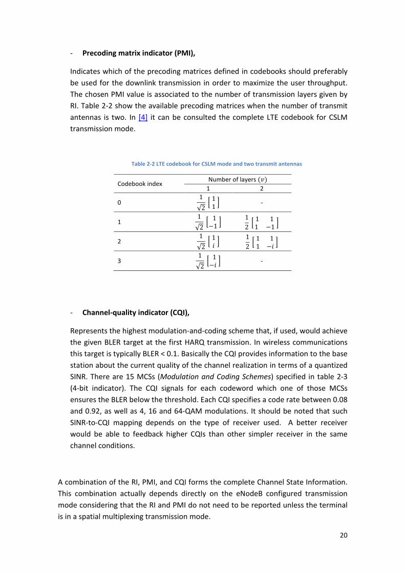
- Precoding matrix indicator (PMI),

Indicates which of the precoding matrices defined in codebooks should preferably

be used for the downlink transmission in order to maximize the user throughput.

The chosen PMI value is associated to the number of transmission layers given by

RI. Table 2-2 show the available precoding matrices when the number of transmit

antennas is two. In [4] it can be consulted the complete LTE codebook for CSLM

transmission mode.

Table 2-2 LTE codebook for CSLM mode and two transmit antennas

Codebook index Number of layers ���

1 2

0 1√2 11 ! -

1 1√2 1−1 !

12 1 11 −1 !

2 1√2 1# !

12 1 1 1 −# !

3 1√2 1−# ! -

- Channel-quality indicator (CQI),

Represents the highest modulation-and-coding scheme that, if used, would achieve

the given BLER target at the first HARQ transmission. In wireless communications

this target is typically BLER < 0.1. Basically the CQI provides information to the base

station about the current quality of the channel realization in terms of a quantized

SINR. There are 15 MCSs (Modulation and Coding Schemes) specified in table 2-3

(4-bit indicator). The CQI signals for each codeword which one of those MCSs

ensures the BLER below the threshold. Each CQI specifies a code rate between 0.08

and 0.92, as well as 4, 16 and 64-QAM modulations. It should be noted that such

SINR-to-CQI mapping depends on the type of receiver used. A better receiver

would be able to feedback higher CQIs than other simpler receiver in the same

channel conditions.

A combination of the RI, PMI, and CQI forms the complete Channel State Information.

This combination actually depends directly on the eNodeB configured transmission

mode considering that the RI and PMI do not need to be reported unless the terminal

is in a spatial multiplexing transmission mode.

21

Table 2-3 Modulation scheme and effective coding rate for each of the Channel Quality Indicators (CQIs)

CQI Index Modulation ERC Data

[bit/symbol]

0 Out of range

1 4-QAM 0.08 0.15

2 4-QAM 0.12 0.23

3 4-QAM 0.19 0.38

4 4-QAM 0.30 0.60

5 4-QAM 0.44 0.88

6 4-QAM 0.59 1.18

7 16-QAM 0.37 1.48

8 16-QAM 0.48 1.91

9 16-QAM 0.60 2.41

10 64-QAM 0.46 2.73

11 64-QAM 0.55 3.32

12 64-QAM 0.65 3.90

13 64-QAM 0.75 4.52

14 64-QAM 0.85 5.12

15 64-QAM 0.93 5.55

The wireless channel is in general time as well as frequency selective and as a result

the most suitable feedback values can vary over consecutive RBs. In transmission, the

eNodeB applies the same CQI value to all RBs assigned to the same user. Even though

the system is configured to calculate a single CQI value for each RB, the base station

would determine an average CQI over the resource blocks assigned to the same user.

On the contrary, the base station can apply different PMI to consecutive RBs

irrespective of the RBs correspond to the same user or not. Due to these factors a

subband CQI and PMI calculation can be highly beneficial in presence of frequency-

selective channels when more than one user is being served.

2.2.2 Transmission modes

SISO : Transmission mode 1

This is the simplest antenna configuration. It consists of one transmit base station that

utilizes a single transmitter antenna and one receive mobile user that also incorporates

one single receiver antenna. Only one stream can be transmitted with single antennas,

which is the reason why only the CQI is needed at the base station.

22

Transmit diversity: Transmission mode 2

Can be applied to any downlink physical channel but is especially useful at

transmissions that cannot be adapted to varying channels conditions by means of link

adaptation, and thus for which diversity is more important. The Alamouti Space-Time

Block Code (STBC) is used to fix the precoding matrix and the number of transmission

layers only depends on the number of transmit antennas. As in the previous case, only

the CQI indicator feedback is needed.

Open Loop Spatial Multiplexing (OLSM): Transmission mode 3

This mode represents a codebook-based precoding scheme that does not rely on any

PMI recommendation from the user and the precoding matrix is also fixed by some

standard in order to achieve multiplexing and/or diversity gain. This mode is mostly

used in high-mobility scenarios where the latency in the PMI reporting is high and an

accurate feedback is difficult to achieve. That is why there is no requirement of

signalling the current precoder used for the downlink transmission. On the other hand

the transmission rank can be adapted and this requires RI and CQI feedback

information.

Since only the RI and CQI are available, OLSM incorporates Cyclic Delay Diversity. This

basically shifts the transmit signal in time direction and transmit these two signals over

different transmit antennas. Since the shifts are inserted cyclically there is no

additional Inter-Symbol Interference. The diversity is increased without additional

receiver complexity because with that process the number of resolvable propagation

paths is higher.

Closed Loop Spatial Multiplexing (CLSM): Transmission mode 4

This is also a codebook-based precoding scheme where the optimum precoding matrix

index is reported by the user, in addition to the RI and CQI. This mode can give gain in

scenarios where the channel does not vary rapidly and there is a low latency in the PMI

reporting, thus accurate feedback information can be achieved. The precoding matrix

is selected from a codebook where the available precoding matrices are indexed. In

order to simplify signalling only the index is sent. Table 2-2 lists the possible precoder

matrices for 2 antennas. For the four antenna case the codebook includes up to 64

precoding matrices.

23

2.2.3 SISO feedback calculation

As commented above no spatial preprocessing is needed in this case. For that reason

the feedback information needed at the base station for a properly transmission is

only the CQI. This choice is based on a mapping between post equalization SINR and

CQI for a SISO AWGN channel. The SINR-to-CQI mapping table was obtained by

simulating the BLER performance for all CQI values. The SINR values in the table are

equal to the AWGN SNRs at 10 % BLER. Once the SINR is estimated at the receiver, it is

compared to the SINR values in the tables and the maximum CQI that allows

transmission without exceeding 10 % BLER is selected. SINR values below the SNR

point obtained from the curve simulated with CQI 1 are mapped to a CQI equal to 20,

which means out of range and whose correspondent spectral efficiency is zero.

Different CQI granularities are supported to give the scheduler the opportunity to

schedule users located in favourable resources, so as to maximize the overall cell

throughput.

2.2.4 MIMO CSLM feedback calculation

In MIMO systems the feedback for link adaptation comprises the three indicators

explained at the beginning of this chapter. If not all these values are used the

optimization with respect to the indicator not employed is omitted and a

corresponding predefined value is used. CQI and PMI can be wideband (if an average

feedback value is calculated over the whole bandwidth) or subband estimated (the

available bandwidth is divided into subbands and different CQI and PMI values are

calculated for each one), and depending on the channel characteristics a specific CQI

and PMI granularity is optimum.

In order to reduce the complexity of the optimization problems in the CSI calculation

described in section 10.4.2 of [5] and in [6] a new sequential optimization is

implemented in the downlink level simulator, studied in detail in [7]. A short

explanation of this estimation is explained below.

The total system bandwidth, consisting of R REs, is divided into S subbands. The set of

REs belonging to subband � is denoted &�. Furthermore a mapping is defined, ρ ∶ )1, … , R, → )1, … S, which assigns a RE r to the corresponding subband s.

The first step consist of finding the optimum subband precoder, 0�. The precoder for

subband s is defined as follows,

0� = 0(1) ∙ 0�(3) (2.1)

24

The rank dependant precoder codebook, defined in [4], is denoted by 4(5). In

equation 2.1 0(1) denotes the wideband precoder and 0�(3) the subband precoder for

subband �.

With the aim to find the preferred subband precoders the spectral efficiency of each

RE 6, denoted 78, is computed for all combinations of precoders (0�) and transmission

ranks (9). This spectral efficiency corresponds to the post-equalization mutual

information, which is calculated by means of the BICM (Bit Interleaved Code

Modulation) capacity with respect to all subband precoders. The BICM capacity is

modulation alphabet dependent and utilizes a function ��:�&� whose envelope

represents the maximum efficiency over all modulation alphabets. Figure 2-5

represents this function [5],

Figure 2-5 BICM capacity of 4, 16 and 64-QAM modulation [4]

��:�&� � max>∈@�>�:�&��2.2�

In this equation, �>�:�&� denotes the BICM capacity with respect to all defined

modulation alphabetsA ∈ B � )BC, B1D, BDC,, which are respectively 4, 16 or 64-

QAM. The estimated spectral efficiency of RE 6 is,

78�0�, 9� � E��:7�&8,F�0���5

FG1�2.3�

Where 9 denotes the transmission rank and 0� the subband precoder. The post-

equalization :7�&8,F calculation is required (the most expensive step because of the

need to compute matrix inversions in order to calculate the receive equalizer filter)

according to,

25

:7�&8,F(0�) = IF ⋅ |�8L�, �M|3∑ IO ⋅OPF |�8L�, #M|3 + RS3 ∑ |T8L�, #M|3O (2.4)

6 V )1, … , &,, � V )1, … , 9,

In equation 2.4 IF denotes the transmit power on layer �, T8 the equalizer on RE 6, IO is the interference caused by the other transmission layers, RS3 the noise power

spectral density and �8L�, #M refers to the element in the �th row and #th column of

matrix �6, which depend on the precoder and is defined as,

�8 = T8�80� � = W(6) , �8 ∈ ℂYZ×Y\ (2.5) where H^ is the channel matrix. Then the sum spectral efficiency for each subband is

maximized in order to choose subband precoders.

7�(0�, 9) = E 78(0�, 9)8_�`

(2.6)

0b�(3)c0(1), 9d = argmaxf̀(g)_ fg(h) 7�(0�, 9) (2.7)

These optimum subband precoders 0b�(3)for each possible transmission rank, 9, and

wideband, :, are stored, as well as the spectral efficiency, 7�, whose sum over all

subbands for each rank is maximized.

7(0�, 9) = E 7�(0�, 9)i�G1

(2.8)

As a result, a first approximation to the preferred rank 9 is found.

9k = argmax5l5mno 7c0b�(9), 9d , 0b�(9) = 0b (1)(9)0b�(3)(9) (2.9)

Afterwards, the RI is obtained by maximization of the sum efficiency over layers. Since

the previous mutual information estimation is not always accurate enough, the sum

efficiency over layers is calculated for 9k and 9k − 1. For each of these ranks and each

layer the equivalent AWGN channels are estimated. Then, an average SINR is

estimated for each subband, values that are mapped to CQIs. Each CQI represents a

certain spectral efficiency, qi, that is summed over layers (CQI parameters are listed in

section 2.2.1) and finally the maximization of the sum efficiency over ranks 9k and 9k − 1 results in the final RI

26

9k , r0b�si, )tu�,i! = argmax ,f(v),f̀(g),` E E q��(0�, t�LwM)xy

�G1i

�G1 (2.10)

Subject to: 9 ≤ 9>|

0(1) V 41(5)

0�(3) V 43(5)

t� V ℳxh× 1

The value tu�LwM denotes the optimal AMC scheme t ∈ ℳ for subband � and

codeword w. In the case of SU-SISO just CQIs are provided per codeword. The preferred

RI equals 9k and the constraint on the number of transmission layers 9 ≤ 9>| follows

from the rank of the channel matrices

9>| = min8 ∈)1,…,�, 6A��(�8) (2.11)

Detailed information about LTE and CQI, PMI and RI calculation can be found in [4], [5]

and [6].

2.3 High velocity consequences

Rayleigh fading is the statistical model used to simulate the propagation effect. It can

be applied in wireless communications when there is no dominant propagation along

the line of sight between the transmitter and the receiver. In a Rayleigh faded channel

the normalized autocorrelation function is expressed by means of the Jake’s model

[10]

&(�) = ��(2����) (2.12)

Where �� denotes a zero order Bessel function of the first kind, �� refers to the

maximum Doppler shift and � is the delay. The product of the maximum Doppler shift

and the delay is known as Normalized Doppler frequency, f�� ,

f�� = ��� with �� = � ��� (2.13)

Where � refers to the user velocity, �� is the carrier frequency and w represents the

speed of light. In Figure 2-6 the behaviour of the normalized autocorrelation function

over normalized Doppler frequency is represented. It can be observed how the

27

temporal correlation decreases, reaching cero at 0.38 normalized Doppler frequency.

Then the correlation fluctuates, never taking values above 0.4.

Figure 2-6 Temporal correlation in a Rayleigh fading channel

Other relevant parameter at high velocity is the channel coherence time, which can be

substantially short compared to the uplink delay in high velocity scenarios. The channel

coherence time is the time duration over which the channel impulse response is

considered to be not varying. According to Clarke’s model ,[11] and [19], the

expression that defines the channel coherence time can be expressed as,

�x = � 916� ��3 ≃ 0.423�� (2.14)

where �� denotes again the maximum Doppler shift. From this expression it can be

seen how an f�� increase, caused by a velocity increase, results in a lower channel

coherence time. When these expressions are evaluated at 2.1 MHz carrier frequency

and 100 km/h (velocity used with SISO antenna configuration) the maximum Doppler

frequency is 194.56 Hz and the channel coherence time is 2.2ms. At 250 km/h (velocity

used for MIMO simulations) the maximum Doppler frequency is 486.45 Hz and the

channel coherence time is 0.87ms. Considering that the uplink delay used in the

simulations is 10ms, the CSI received at the base station can be assumed completely

outdated information and virtually uncorrelated with respect to the current channel

conditions.

10−2

10−1

100

0

0.1

0.2

0.3

0.4

0.5

0.6

0.7

0.8

0.9

1

Normalized Doppler frequency

Cor

rela

tion

28

Figure 2-7 SINR variation between consecutive subframes at high velocity

In Figure 2-7 the post-equalization SINR calculated in the receiver is represented over

time. Strong and fast fluctuations in the channel conditions are the cause of these

SINR variations, which can be more than 20dB between consecutive subframes.

The user performance obtained with the same simulation parameters in terms of

throughput and BLER can be seen in Figure 2-8. The results show an important loss in

throughput, with respect to the results obtained by applying the original algorithm

with zero UL delay, as well as a BLER exceeding the 0.1 target.

Figure 2-8 Performance loss due to the feedback delay

0 100 200 300 400 500−25

−20

−15

−10

−5

0

5

10

15

20

25SINR variation over time

Number of subframes

SIN

R [d

B]

−10 −5 0 5 10 15 200

0.5

1

1.5

2

2.5

3

3.5

4

4.5

SNR [dB]

Thr

ough

put [

Mbi

t/s]

SU−SISO Throughput, 100 km/h

0ms uplink delay10ms uplink delay

−10 −5 0 5 10 15 200

0.1

0.2

0.3

0.4

0.5

0.6

0.7

0.8

0.9

SNR [dB]

BLE

R

SU−SISO BLER, 100 km/h

0ms uplink delay10ms uplink delay

29

2.4 Vienna LTE simulators

In the past few years reproducible research has been an important objective in the

field of signal processing, and even more important as the simulated systems become

more and more complex. This is the case for wireless communication systems.

Researchers often demand to access the original source code to reproduce and verify

the results presented. The Vienna LTE simulators, as an open source software

plataform, are a very important tool to carry out these verifications.

The Vienna LTE simulator is a standard-compliant open-source Matlab-based

simulation platform, which supports link and system level simulations and that

implements UMTS LTE.

Link level simulations are used to investigate e.g. channel estimation, tracking,

prediction and synchronization algorithms, MIMO gains, AMC (Adaptive

Modulation and Coding), feedback techniques, receiver structures and channel

modelling.

System level simulations are used to investigate network issues, such as

resource allocation and scheduling, multi-user handling, mobility management,

admission control, interference management and network planning

optimization. A network consists of multiple eNodeBs that cover a specific area

in which many mobile terminals are located or moving around.

The complete structure of these simulators is explained in [12] and [13]. In these

papers it is also explained how link and system level are connected, because the

former serves as a reference for designing the latter. Moreover, the wide capabilities

of the simulator can be observed through some examples of its application.

To be able to investigate different feedback algorithms implemented during this thesis,

all the simulations are performed in the downlink link level simulator.

The link level simulator consists of three building blocks, namely, transmitter, channel

model and receiver that are represented in Figure 2-9 [12].

- Transmitter. Based on UE feedback the scheduler assigns the available RBs to

UEs, setting the appropriate MCS, transmission mode and precoding/number of

spatial layers.

- Channel model. This simulator supports block and fast-fading channels. The

available channel models are AWGN, flat Rayleigh fading, Power Delay Profile-

based such as ITU Pedestrian A/B or ITU Vehicular A/B, TU (Typical Urban) and

Winner II among others.

30

- Receiver. The simulator supports ZF (Zero Forcing), LMMSE (Linear Minimum

Mean Squared Error) and SSD (Soft Sphere Decoding) as detection algorithms.

After detection the channel is estimated and the feedback indicators are

calculated.

Figure 2-9 Downlink link level simulator architecture

In a downlink transmission, the data is generated in the transmitter, sent through the

channel model and detected at the receiver. The channel model introduces signal

distortions, such as time- and frequency-selective fading. . This data contains signalling

information, i.e. coding, HARQ, scheduling and precoding parameters that are

assumed to be error-free due to the low coding rates and low order modulation

utilized.

The uplink signalling and feedback transmission are also assumed error-free. The only

considered distortion is a delay in the feedback path.

2.4.1 Main simulation parameters

In table 2-4 the main simulation parameters that remains constant during all the

simulations can be found.

Table 2-4 Constant simulation parameters

Carrier frequency 2.1 GHz

System bandwidth 1.4 MHz

Subcarrier spacing 15 kHz

Receiver Zero forcing (ZF)

Channel model Block fading

Channel estimation Perfect

Number of eNodeBs 1

31

For both the development of the methods that estimate the CQI and the comparison

of them over SNR, it is employed a scenario with unfavorable characteristics. The

simulation parameters appear in table 2-5.

Table 2-5 Simulation parameters utilized do develop the methods to estimate the CQI

Transmission mode 1

Channel model Flat Rayleigh

UL delay 10 ms

Number of users 1

In order to compare the methods that estimate the CQI over the normalized Doppler

frequency the following simulation parameters in table 2-6 are used.

Table 2-6 Simulation parameters utilized to compare the CQI methods over ���

Transmission mode 1

Channel model Flat Rayleigh correlated

UL delay 1 ms

Number of users 1

User velocity Variable (0-300 km/h)

The sections where the PMI and RI are investigated utilize the simulation parameters

written in table 2-7.

Table 2-7 Simulation parameters in order to study PMI and RI

Transmission mode 4

Channel model Flat Rayleigh

UL delay 10 ms

Number of users 1

Rx antenna correlation 0.5 (Kronecker model)

32

Finally when the methods are evaluated using a frequency selective channel the

parameters in table 2-8 are applied.

Table 2-8 Simulation parameters to evaluate the methods in a frequency selective channel

Transmission mode 4

Channel model Flat Rayleigh correlated

UL delay 1 ms

Number of users 6

User velocity Variable (0-300 km/h)

33

34

3. FEEDBACK ALGORITHMS TO IMPROVE THE USER

THROUGHPUT

In this chapter, the new algorithms designed to improve the throughput in high

mobility scenarios are presented. These algorithms are implemented without being

concerned about the BLER resuslts, which are above 10% in most of the cases. It is

expected that in practice, applying the HARQ process, the BLER target will be achieved.

3.1 Study of the CQI

3.1.1 SINR Long-term average

The first step in this method consists of changing the SINR mapping table to obtain the

maximum possible throughput. With the feedback deactivated, the throughput curves

for each CQI are simulated over SNR and applying the parameters in table 2-5. Then a

new mapping table is created by selecting the SNR points that achieve the maximum

throughput for each CQI. Figure 3-1 represents the maximum throughput achieved for

each CQI separately.

Figure 3-1Maximum throughput curves for CQI 1-15

In addition, this method estimates an SINR long-term average at the receiver. Several

methods that calculate the average of some parameters over time have been studied

−10 −5 0 5 10 15 20 25 300

0.5

1

1.5

2

2.5

3

3.5

4

4.5

5

SNR [dB]

Thr

ough

put [

Mbi

t/s]

TP curves for each CQI

CQI=1CQI=2CQI=3CQI=4CQI=5CQI=6CQI=7CQI=8CQI=9CQI=10CQI=11CQI=12CQI=13CQI=14CQI=15

35

before, two examples can be found in [14] and [15]. The expression employed in this

method is the Exponentially Weighted Moving Average (EWMA), a type of infinite

impulse response filter that applies weighting factors which decrease exponentially.

The weighting for each older datum decreases exponentially, never reaching zero.

:7�&�������S = �1 − 1�� :7�&�������S�1 + � 1�� :7�&S (3.1)

In that expression the parameter � defines the weight factors applied to the

instantaneous :7�&S and the previous averaged :7�&�������S�1. The larger is beta, the

smaller weight factor is applied to the current SINR value. Beta value is chosen by

simulations, and in this case where there is no temporal correlation a value beta equal

to 10 is employed. Smaller beta values result in lower throughput while larger beta

values result in the same performance.

3.1.2 Maximum throughput expected

This method consists of trying to learn the CQI statistics, which are a-priori unknown to

the user. Based on these CQI statistics, the expected throughput is estimated and

maximized with respect to the CQI. An scheduling method that maximizes the

throughput with adjustable fairness is detailed in [16]. Similar expressions are applied

here to calculate the maximum throughput expected.

At each realization an instantaneous approximation of the CQI probability mass

function (pmf) is estimated with the CQI calculated for the current channel conditions,

denoted ��7S. This ��7S value has been calculated through mapping the

instantaneous :7�&S.

�S(#) = 1& E 1 L��7S(6) = #M # V 1, … , �@�x�

8G1 (3.2)

In this expression i as well as R denote the number of available modulation and coding

schemes. The only non-zero value in this vector, �S(#) , is located in the position

whose index is equal to the ��7S selected by the algorithm. Then this vector is

averaged over time employing the same type of exponential averaging filter as in the

previous method, i.e., EWMA.

�̂S = �1 − 1�� �̂S�1 + �1�� �S (3.3)

36

�̂S indicates the probability that a given CQI is instantaneously optimal. The beta value

is again chosen by simulations, selecting as in the previous method beta equal to 10.

After that the expected throughput is estimated for each CQI "i", as the product of the

spectral efficiency of CQI "i" and the probability that the channel supports this CQI, i.e.,

the sum of the probabilities of all CQIs larger than or equal to "i"

��|�(��7O) = ���#w#��w�(��7O) ∙ E �̂S(w�#)��O�x� ¡

# ∈ 1, … , �@�x (3.4)

Finally the CQI with highest expected throughput is selected to be fed back over the

uplink channel.

3.1.3 Conditional CQI probability

This method estimates the CQI that maximizes the throughput based on the

knowledge of the probability of the UE to choose a specific CQI when the previous CQI

selected is known.

For that purpose, the probability of a specific CQI to be selected depending on the

previous CQI employed is needed. These probabilities are calculated in first place

storing in a squared matrix, of length the number of modulation and coding schemes,

the number of times that a specific CQI is selected. The matrix indexes where the

instantaneous CQI, denoted ��7S , is stored at each realization are given in the first

dimension by the CQI value calculated in the previous realization, denoted ��7S�1 ,

and in the second dimension by the current ��7S. Figure 3-2 is an example of the data

matrix at 100km/h, 10dB SNR, 10ms uplink delay and 1000 simulated subframes. For a

specific previous CQI, it can be seen how many times each CQI has been chosen at the

next realization.

Once these data has been stored in a matrix, the probability vectors for each ��7S�1

(previous CQI) are estimated. Each value of this matrix is divided by the sum of the

number of CQIs stored in the row that it occupies. The result is a matrix that consists of �@�x probability vectors, which indicate the probability of a specific CQI to be selected

depending on the previous CQI.

37

Figure 3-2 CQI dependant on the previous CQI

Once this probability vectors are available the method can be applied. At each

realization one instantaneous CQI, ��7S , is estimated through SINRS mapping.

Moreover, the CQI selected in the previous realization, ��7S�1, is also known because

it has been stored. This ��7S�1 is used to index the row of the matrix previously

calculated, obtaining a probability vector denoted as �x� ¤¥v.

Finally the throughput expected is calculated using the same expression as in the

previous method (equation 3.4), employing as �̂S the probability vector indexed by

��7S�1, that is, �x� ¤¥v. Finally the CQI that maximizes the expression is fed back over

the uplink channel.

The main disadvantage of this method is that it is necessary to store the CQIs selected

over time to calculate the correspondent probability vectors before applying the

method. Moreover, this data matrix has to be calculated for each specific speed, SNR

point and uplink delay, resulting in an excessive computational cost.

3.1.4 SINR variation

With the goal of simplifying this method, a new procedure is implemented based on

the same idea. It basically consists of storing in a vector, whose length increases with

the number of simulated subframes, the SINR variation between consecutive

subframes over time. At each realization the probability distribution of the stored

SINR variation values up to that time is fitted by a t location-scale distribution function,

which is denoted as I�∆:7�&�. The t location-scale distribution is useful for

modelling data with heavier tails (more prone to outliers) than the normal distribution.

38

−40 −30 −20 −10 0 10 20 30 400

10

20

30

40

50

60T location scale distribution, 100 Km/h

SNR variation [dB]−40 −30 −20 −10 0 10 20 30 400

10

20

30

40

50

60

SINR variation [dB]

T location scale distribution, 50 Km/h

Figure 3-3 represents an example of the SINR variation distribution setting 10dB SNR,

10ms uplink delay, 1000 simulated subframes and at 100km/h and 50km/h,. The

lower the velocity, the narrower and picked the distribution becomes because the

SINR variations are less pronounced.

Figure 3-3 T location-scale distribution function

Then the difference between the instantaneous SINR, denoted as :7�&S, and the

necessary SINR to select each different CQI, :7�&(��7O), is estimated. :7�&(��7O) is

a vector whose values correspond to the values in the mapping table.

∆:7�&S(#) = :7�&S − :7�&(��7O) # ∈ 1, … , �B¦� (3.5)

As a result, a vector of necessary SINR variations, ∆:7�&S(#), of length the number of

modulation schemes, �@�x , is obtained.

After that, and for each possible CQI, the probability than the SINR variations will be

above the values calculated in equation 3.5 are estimated. These probabilities are

computed using the complementary cumulative distribution function (ccdf), which

corresponds to the upper probability tail of the t location-scale distribution function

for each ∆:7�&S(#) value

�̂S(#) = Ic∆:7�& > ∆:7�&S(#)d # ∈ 1, … , �B¦� (3.6)

This probability vector is used as in the previous methods to calculate the expected

throughput for each possible CQI. Finally the CQI that maximizes equation 3.7 is fed

back over the uplink channel.

��|�(��7O) = ���#w#��w�(��7O) ∙ E �̂S(w�#)��O�x� ¨

# ∈ 1, … , �@�x (3.7)

39

−10 −5 0 5 10 15 200

0.5

1

1.5

2

2.5

3

3.5

4

4.5

SNR [dB]

Thr

ough

put [

Mbi

t/s]

UE throughput

Zero uplink delay, Original feedback method10ms uplink delay, Original feedback method10 ms uplink delay, SINR Long−term average10 ms uplink delay, Maximum expected throughput10 ms uplink delay, SINR variation

−10 −5 0 5 10 15 2010

−2

10−1

100

SNR [dB]

BLE

R

UE BLER

Zero uplink delay, Original feedback method10ms uplink delay, Original feedback method10 ms uplink delay, SINR Long−term average10 ms uplink delay, Maximum expected throughput10 ms uplink delay, SINR variation

3.1.5 Methods comparison and adaptation to different velocity

In Figure 3-4 a comparison between the results obtained simulating the methods

presented in this chapter is shown. The simulation parameters applied are written in

table 2-5.

Figure 3-4 Throughput improvement methods comparison

The throughput results using the SINR Long term average method and Maximum

expected throughput method are very similar, achieving an important improvement.

With the SINR variation method there is also throughput improvement, nevertheless,

not as large as with the previous ones. This happens due to the fact that the t location-

scale distribution function does not fit the SINR variation sufficiently proper, and the

probability vectors obtained are not accurate enough.

With regard to the BLER, the lower values are reached using the SINR long-term

average method, which even improves the results obtained with the original method

in most of the SNR points. In the other two cases there is only BLER improvement at

high SNR.

METHODS EVALUATION OVER NORMALIZED DOPPELR FREQUENCY

In order to know the range of velocities and uplink delays where the methods

explained before can work properly, some comparisons are simulated over normalized

Doppler frequency. The simulation parameters are written in table 2-6. Figure 3-5

shows the results when the uplink delay is fixed to 1 ms, beta is fixed to 10 and the

velocity varies from 0 to 300km/h.

40

Figure 3-5 SISO Throughput over normalized Doppler Frequency and beta = 10

When the velocity is not severely high (up to 0.1 Normalized Doppler that corresponds

to ≈50 km/h with the simulation parameters used), the temporal channel correlation is

strong and it is not necessary to estimate an average of the SINR and the CQI, the

original feedback method works properly.

The expressions used to average the SINR and the CQI in the SINR long-term average

and Maximum throughput expected methods depend on the parameter � (equation

3.1 y 3.3). This parameter � defines the weight factors applied to the instantaneous

and the previous averaged channel characteristics and can be adapted depending on

the normalized Doppler frequency. Through simulations of these methods applying

different beta parameter has been concluded that up to 0.1 normalized Doppler

frequency the highest performance is achieved by setting beta equal to 1, which

means no average. On the contrary, from 0.1 normalized Doppler frequency the

temporal channel correlation decreases substantially fast and the best performance is

achieved using a larger beta value. The most appropriate beta is equal to 10 because it

achieves higher throughput than with lower beta values, nevertheless not higher than

with larger values.

� = © 1 �# f�� ≤ 0.1 10 �# f�� > 0.1 (3.8)

The last investigation in this chapter is a comparison between the adapted methods

and a linear predictor. The linear predictor basically calculates a linear interpolation of

the previous channel realizations that are stored in a predictor buffer. Then an

10−2

10−1

100

1.4

1.6

1.8

2

2.2

2.4

2.6

2.8

3

Normalized Doppler frequency

Thr

ough

put [

Mbi

t/s]

UE throughput

Original feedback methodSINR long−term averageMaximum expected throughput

41

extrapolation of these data gives a prediction of the current channel, therefore

temporal correlation between consecutive subframes is essential.

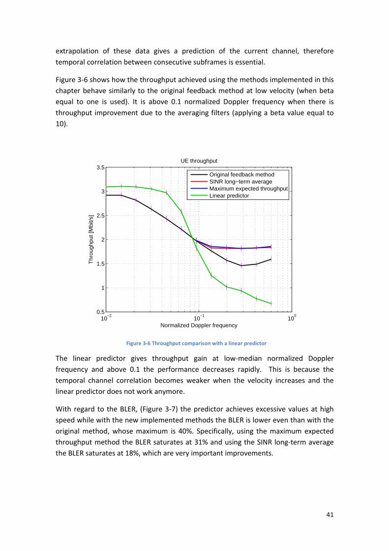
Figure 3-6 shows how the throughput achieved using the methods implemented in this

chapter behave similarly to the original feedback method at low velocity (when beta

equal to one is used). It is above 0.1 normalized Doppler frequency when there is

throughput improvement due to the averaging filters (applying a beta value equal to

10).

Figure 3-6 Throughput comparison with a linear predictor

The linear predictor gives throughput gain at low-median normalized Doppler

frequency and above 0.1 the performance decreases rapidly. This is because the

temporal channel correlation becomes weaker when the velocity increases and the

linear predictor does not work anymore.

With regard to the BLER, (Figure 3-7) the predictor achieves excessive values at high

speed while with the new implemented methods the BLER is lower even than with the

original method, whose maximum is 40%. Specifically, using the maximum expected

throughput method the BLER saturates at 31% and using the SINR long-term average

the BLER saturates at 18%, which are very important improvements.

10−2

10−1

100

0.5

1

1.5

2

2.5

3

3.5

Normalized Doppler frequency

Thr

ough

put [

Mbi

t/s]

UE throughput

Original feedback methodSINR long−term averageMaximum expected throughputLinear predictor

42

Figure 3-7 BLER comparison with a linear predictor

The utilized method should depend on the normalized Doppler frequency, selecting

the linear predictor up to 0.1 and the SNR Long-Term Average or the Maximum

throughput expected method above that value.

3.2 Study of the RI and PMI

In this section the proposed adapted methods are evaluated by using MIMO antenna

configurations. As explained in the theory, when multiple antennas are used in the

transmitter and the receiver a pre-transmission spatial preprocessing of the data is

necessary because several spatial streams are formed. The spatial preprocessing at the

eNodeB depends on the rank indicator and the precoding matrix indicator that are

calculated in the receiver.

The modifications that are applied to the original feedback method are explained

below.

10−2

10−1

100

10−3

10−2

10−1

100

Normalized Doppler Frequency

BLE

R

UE BLER

Original feedback methodSINR long−term averageMaximum expected throughputLinear predictor

43

3.2.1 CSLM Code modifications

- CQI selection: When there are multiple antennas in the transmitter and in the

receiver the CQI adaption method should be calculated separately for each

layer, applying different SINR long-term averaging filters. However, this does

not increase significantly the computational cost with respect to the original

feedback algorithm.

- PMI selection: In the original code this indicator is calculated by maximization

of the post-equalization mutual information for each subband, as explained in

section 2.2.4. The mutual information can be seen as a measure of the

instantaneous channel capacity, whose estimation depends on the SINR. In

turn, the SINR estimation depends on the precoding matrix used at each

realization.

Due to the high velocity that means a short channel coherence time and the

large uplink delay, the post-equalization mutual information is not an accurate

measure. This is because the PMI calculated at each time instant could not be

optimum at the moment of its aplication. The best option is to fix a specific

indicator and to use always the same precoding matrix in case the feedback

delay is large compared to the channel coherence time.

- RI selection: In the legacy feedback algorithms a first approximation of the rank

indicator 9k is obtained by maximization of the post-equalization mutual

information with respect to the possible ranks. Nevertheless, the final indicator

is selected between 9k and 9k − 1 by maximization of the sum efficiency.

In the type of scenarios where the simulations are performed, the mutual

information is not an appropriate measure, as explained above, so it is not

estimated. Instead of the mutual information, the sum efficiency over layers for

every possible rank is calculated and maximized, obtaining a first

approximation of 9k . This RI value tends to fluctuate over consecutive

realizations, once again due to the channel variations, and the maximum

throughput is not always achieved. In order to smooth these fluctuations a

simple algorithm is implemented. It basically consists of storing in a vector the

last � RI values calculated by the algorithm, selecting as the final RI the

majority of the stored values.

44

3.2.2 Results

The first configuration studied is the one with the minimum number of antennas in the

transmitter and the receiver, but more than one layer, which is 2x2 Single User MIMO

(two antennas in both transmitter and receiver). The rest of the simulation parameters

utilized are written in table 2-7. An important goal of the design in MIMO is that the

different antennas should not be spatially correlated in order to exploit the diversity.

The performance obtained with the original feedback method and without antenna

correlation is represented in Figure 3-8.

Figure 3-8 2x2 MIMO, Zero antenna correlation

It can be seen that the throughput achieved at low SNR is very similar for rank 1 and

rank 2. In order to investigate about RI selection, 0.5 receiver antenna correlation is

introduced to make this RI decision more difficult for the algorithm. In Figure 3-9 it is

shown how the gap between rank 1 and 2 increases when 0.5 receiver antenna

correlation is applied. This happens because the spatial correlation correlates the

signals received over the received antennas, which basically implies that the largest

singular value of the channel matrix grows, while the other singular values become

smaller. As a result we obtain an increased SNR gap between rank 1 and the rest of the

transmission ranks.

−10 −5 0 5 10 15 20 25 300

1

2

3

4

5

6

7

8

9

SNR [dB]

Thr

ough

put [

Mbi

t/s]

UE throughput

Rank 1Rank 2Original feedback method

45

Figure 3-9 2x2 SU-MIMO throughput with 0.5 receiver antenna correlation

Now, with receiver correlation, is possible to observe how the CQI feedback method

works properly when the performance is calculated for each rank separately, however,

when the original RI adaptation is applied (green line) the performance decreases

significantly between 15 and 30 dB because the algorithm does not select the optimum

RI because of its fluctuations over time.

Figure 3-10 2x2 SU-MIMO throughput improvement with 0.5 antenna correlation

In Figure 3-10 the SINR long-term average method is applied firstly to each layer

separately, obtaining the results represented by blue lines. Then the algorithm for RI

adaptation that estimates the majority of the previous values selected is applied,

obtaining the throughput represented by the red line. Although the RI majority is used,

between 20 and 30 dB the number of times that the original method selects rank one

and rank two is about 50%, as a result, even the majority value fluctuates in that SNR

−10 −5 0 5 10 15 20 25 30 350

1

2

3

4

5

6

7

8

9

SNR [dB]

Thr

ough

put [

Mbi

t/s]

UE throughput

Original feedback method, Rank 1, 2Original adaptive feedback method

−10 −5 0 5 10 15 20 25 30 350

1

2

3

4

5

6

7

8

9

SNR [dB]

Thr

ough

put [

Mbi

t/s]

UE throughput, 0,5 receiver antenna correlation

Original feedback method, Rank 1, 2Original feedback methodSINR long−term average, Rank 1, 2SINR long−term average

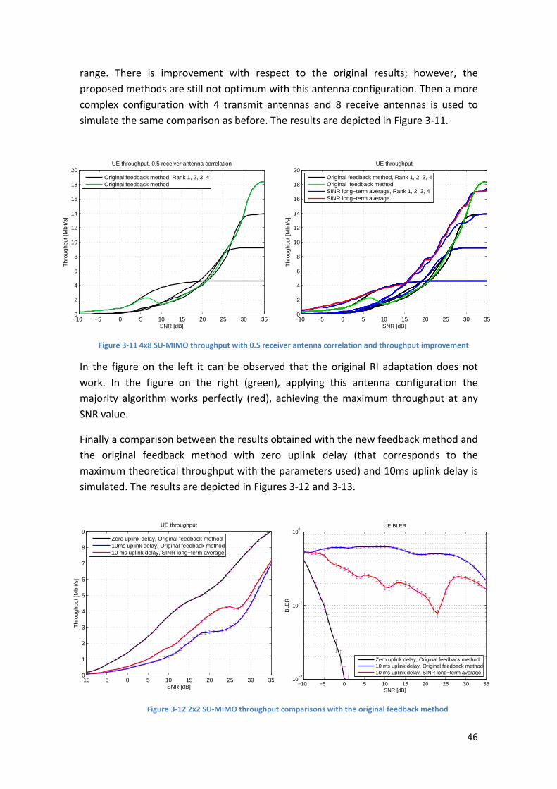
46

−10 −5 0 5 10 15 20 25 30 350

1

2

3

4

5

6

7

8

9

SNR [dB]

Thr

ough

put [

Mbi

t/s]

UE throughput

Zero uplink delay, Original feedback method10ms uplink delay, Original feedback method10 ms uplink delay, SINR long−term average

−10 −5 0 5 10 15 20 25 30 3510

−2

10−1

100

SNR [dB]

BLE

R

UE BLER

Zero uplink delay, Original feedback method10 ms uplink delay, Original feedback method10 ms uplink delay, SINR long−term average

−10 −5 0 5 10 15 20 25 30 350

2

4

6

8

10

12

14

16

18

20

SNR [dB]

Thr

ough

put [

Mbi

t/s]

UE throughput, 0.5 receiver antenna correlation

Original feedback method, Rank 1, 2, 3, 4Original feedback method

−10 −5 0 5 10 15 20 25 30 350

2

4

6

8

10

12

14

16

18

20

SNR [dB]

Thr

ough

put [

Mbi

t/s]

UE throughput

Original feedback method, Rank 1, 2, 3, 4Original feedback methodSINR long−term average, Rank 1, 2, 3, 4SINR long−term average

range. There is improvement with respect to the original results; however, the

proposed methods are still not optimum with this antenna configuration. Then a more

complex configuration with 4 transmit antennas and 8 receive antennas is used to

simulate the same comparison as before. The results are depicted in Figure 3-11.

Figure 3-11 4x8 SU-MIMO throughput with 0.5 receiver antenna correlation and throughput improvement

In the figure on the left it can be observed that the original RI adaptation does not

work. In the figure on the right (green), applying this antenna configuration the

majority algorithm works perfectly (red), achieving the maximum throughput at any

SNR value.

Finally a comparison between the results obtained with the new feedback method and

the original feedback method with zero uplink delay (that corresponds to the

maximum theoretical throughput with the parameters used) and 10ms uplink delay is

simulated. The results are depicted in Figures 3-12 and 3-13.

Figure 3-12 2x2 SU-MIMO throughput comparisons with the original feedback method

47

−10 −5 0 5 10 15 20 25 30 350

2

4

6

8

10

12

14

16

18

20

SNR [dB]

Thr

ough

put [

Mbi

t/s]

UE throughput

Zero uplink delay, Original feedback method10ms uplink delay, Original feedback method10 ms uplink delay, SINR long−term average

−10 −5 0 5 10 15 20 25 30 3510

−2

10−1

100

SNR [dB]

BLE

R

UE BLER

Zero uplink delay, Original feedback method10 ms uplink delay, Original feedback method10 ms uplink delay, SINR long−term average

Figure 3-13 4x8 SU-MIMO throughput comparisons with the original feedback method

The figures on the left show throughput improvement with respect to the results

obtained using the original feedback method with 10 ms uplink delay when the SINR

long-term average method is simulated. Furthermore, BLER improvement can also be

observed in the figures on the right. These improvements increase with the use of

more complex antenna configurations.

3.3 Frequency-selective channel with multiple users

During the work presented up to now, where a flat fading channel and only one user

have been simulated, the calculation of the CQI and PMI have been wideband, i.e., an

average of the channel characteristics over the whole bandwidth has been estimated

and the same indicator values have been reported over all RBs.

In this section the performance obtained when simulating a time and frequency

selective channel with multiple users is studied. In section 2.2.4 the feedback

indicators calculation is detailed. It is possible to estimate either wideband or subband

CQI and PMI indicators, depending on the CQI and PMI granularity configured in the

simulator. An average CQI/ PMI over the whole available bandwidth is estimated in

case the granularity is set to six. On the other hand, different CQI and/or PMI are

estimated for each subband when the granularity is configured to one. Considering

that the total bandwidth used in the simulations is 1.4 MHz and the subcarrier spacing

selected is 15 kHz, the bandwidth assigned to each RB is 180 KHz, being also this value

the minimum subband bandwidth. In this study the four possible combinations of CQI

48

and PMI granularities six and one are simulated. The simulation parameters are

available in table 2-8, moreover, four transmitter antennas and two receiver antennas

are used.

The scheduling strategy used in this section that allows assigning the physical

resources to the users is Maximum Rate. The goal of this strategy is to maximize the

system throughput taking the scheduling decisions according to the reported channel

quality. It tries to transmit to users with favorable radio-link conditions, which allows

obtaining multi-user-diversity gain.

The solid lines in Figure 3-14 represent the cell throughput obtained using the original

feedback method. At low f�� the highest performance is achieved with CQI and PMI

granularity one due to the high temporal channel correlation. Above 0.1 f�� the

performance decrease rapidly and it is from this point where the new feedback

method implemented that calculates an SINR average achieves the highest

performance.

In order to study the range of normalized Doppler frequency where the PMI

adaptation obtains throughput improvement using the SINR long-term average

method, the PMI feedback has been activated during the simulations in this section.

The lines with circles represent the results of setting the four possible PMI and CQI

granularity combinations of one and six and using the SINR long-term average method.

Figure 3-14 Cell throughput improvement using SINR long-term average method

10−2

10−1

100

0

1

2

3

4

5

6

7

8

9

Normalized Doppler Frequency

Thr

ough

put [

Mbi

t/s]

Cell throughput

CQI 1, PMI 1CQI 1, PMI 1, SINR−long term averageCQI 1, PMI 6CQI 1, PMI 6, SINR−long term averageCQI 6, PMI 1CQI 6, PMI 1, SINR−long term averageCQI 6, PMI 6CQI 6, PMI 6, SINR−long term averageCQI 1, PMI fixed, SINR long−term average

49

From f�� equal to 0.1 up to 0.3 the highest performance using the new feedback

method is still achieved with PMI granularity one, however, from 0.3 f�� it can be seen

how the results are very similar irrespective of the indicators granularity. This

behaviour is due to the fact that the channel variations become extremely fast and the

SINR average over consecutive RBs stays practically flat. The same occurs with the

BLER results, which are shown in Figure 3-15.

Finally the SINR long term average method has been simulated from 0.1 f�� with CQI

granularity equal to one and fixed PMI. The result corresponds to the red line with

crosses. In Figure 3-14 it can be observed that from around 0.3 f�� the throughput

achieved is even higher than using the original feedback method. Nevetheless, this is

not the only improvement, for the same f�� range the BLER decreases considerably,

from 40% with adaptive PMI to 26% with fixed PMI, as depicted in 3-15.

Figure 3-15 Cell BLER improvement using SINR long-term average method

10−2

10−1

100

10−2

10−1

100

SNR [dB]

BLE

R

Cell BLER

CQI 1, PMI 1CQI 1, PMI 1, SINR−long term averageCQI 1, PMI 6CQI 1, PMI 6, SINR−long term averageCQI 6, PMI 1CQI 6, PMI 1, SINR−long term averageCQI 6, PMI 6CQI 6, PMI 6, SINR−long term averageCQI 1, PMI fixed, SINR long−term average

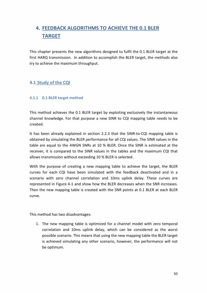
50

4. FEEDBACK ALGORITHMS TO ACHIEVE THE 0.1 BLER

TARGET

This chapter presents the new algorithms designed to fulfil the 0.1 BLER target at the

first HARQ transmission. In addition to accomplish the BLER target, the methods also

try to achieve the maximum throughput.

4.1 Study of the CQI

4.1.1 0.1 BLER target method

This method achieves the 0.1 BLER target by exploiting exclusively the instantaneous

channel knowledge. For that purpose a new SINR to CQI mapping table needs to be

created.

It has been already explained in section 2.2.3 that the SINR-to-CQI mapping table is

obtained by simulating the BLER performance for all CQI values. The SINR values in the

table are equal to the AWGN SNRs at 10 % BLER. Once the SINR is estimated at the

receiver, it is compared to the SINR values in the tables and the maximum CQI that

allows transmission without exceeding 10 % BLER is selected.

With the purpose of creating a new mapping table to achieve the target, the BLER

curves for each CQI have been simulated with the feedback deactivated and in a

scenario with zero channel correlation and 10ms uplink delay. These curves are

represented in Figure 4-1 and show how the BLER decreases when the SNR increases.

Then the new mapping table is created with the SNR points at 0.1 BLER at each BLER

curve.

This method has two disadvantages:

1. The new mapping table is optimized for a channel model with zero temporal

correlation and 10ms uplink delay, which can be considered as the worst

possible scenario. This means that using the new mapping table the BLER target

is achieved simulating any other scenario, however, the performance will not

be optimum.

51

2. In chapter 2 has been explained that due to the correlation and uplink delay

parameters used it is not appropriate to take into account exclusively

instantaneous channel conditions because the CQI estimated is not optimum at

the moment of its application.

Figure 4-1 BLER curves for CQI 1-15 with zero correlation and 10ms uplink delay

4.1.2 Expected BLER method

The goal of this algorithm is once again to maintain the BLER values below 10% and at

the same time to solve the drawbacks that the previous method presents. By using this

method, the 0.1 BLER target is achieved with any correlation and uplink delay

parameters, besides, it also tries to achieve the highest throughput by taking

advantage of the channel statistics.

The method involves estimating the expected BLER for each possible modulation and

coding scheme, selecting the highest CQI that achieves the target. The AWGN SNR-

BLER curves obtained with optimum channel conditions (high temporal correlation and

zero uplink delay) are employed for that purpose. These curves are depicted in Figure

4-2.

−10 −5 0 5 10 15 20 25 30

0.1

0.2

0.3

0.4

0.5

0.6

0.7

0.8

0.9

1

SNR [dB]

BLE

R

AWGN BLER curves for cqi 1−15, 100km/h, 10ms uplink delay

52

The first step consists of storing in a vector the instantaneous SINR values obtained

during the last � realizations.

ªS = L:7�&S, :7�&S�1, :7�&S�3, … , :7�&S�«M (4.1)

Once these values are known, all of them are evaluated over each BLER curve

separately, calculating an average and obtaining the BLER expected result for each

possible CQI.

¬­q&�®�(��7O) = 1¯°�±#ª²³(ªS) E ¬­q&x� ¡c:�&S�´d«´G�

(4.2)

In equation 4.2 ¬­q&x� ¡ represents the specific BLER curve obtained with CQI “i”.

Finally the CQI with highest BLER expected below 0.1 is selected.

Figure 4-2 BLER curves for CQI 1-15 with maximum correlation and zero uplink del

4.1.3 Methods comparison and evaluation over normalized Doppler frequency

Figure 4-3 represents a comparison between the results obtained applying the original

feedback method and the previous methods explained in this chapter that achieve the

BLER target. The simulation parameters are available in table 2-5.

−10 −5 0 5 10 15 20 250

0.1

0.2

0.3

0.4

0.5

0.6

0.7

0.8

0.9

1

SNR [dB]

BLE

R

Original AWGN BLER curves for CQI 1−15

53

−10 −5 0 5 10 15 20 25 300

1

2

3

4

5

6

SNR [dB]

Thr

ough

put [

Mbi

t/s]

UE throughput

Zero uplink delay, original feedback method10ms uplink delay, original feedback method10ms uplink delay, 0.1 BLER target method10ms uplink delay, Expected BLER method

−10 −5 0 5 10 15 20 25 3010

−2

10−1

100

SNR [dB]

BLE

R

UE BLER

Zero uplink delay, original feedback method10ms uplink delay, original feedback method10ms uplink delay, 0.1 BLER target method10ms uplink delay, Expected BLER method

10−2

10−1

100

0.5

1

1.5

2

2.5

3

Normalized Doppler Frequency

Thr

ough

put [

Mbi

t/s]

UE throughput

Original feedback method0.1 BLER target methodExpected BLER method

10−2

10−1

100

10−3

10−2

10−1

100

Normalized Doppler Frequency

BLE

R

UE BLER

Original feedback method0.1 BLER target methodExpected BLER method

The figure on the right represents the BLER in the receiver. The results show a BLER

remaining below 0.1 when the new methods implemented are used; however, in the

figure on the left it is shown that the throughput has decreased, especially when using

the 0.1 BLER target method that only exploits the instantaneous SINR values.

Figure 4-3 Methods comparison that achieve the 10% BLER

Afterwards, the methods are evaluated over the normalized Doppler frequency

applying the simulation parameters in table 2-6. It is shown on the right of Figure 4-4

that with the BLER expected method the BLER target is fulfilled at any f�� while

improving the throughput with respect to the 0.1 BLER target method. On the contrary

with the original method the BLER increases with the velocity, up to 0.4, a considerable

high value.

Figure 4-4 Methods comparison that achieve 10% BLER over ���

54

−10 0 10 20 30 400

1

2

3

4

5

6

7

8

9

SNR [dB]

Thr

ough

put [

Mbi

t/s]

UE throughput

0.1 BLER target method, Rank 1, 20.1 BLER target methodExpected BLER method, Rank 1, 2Expected BLER method

−10 0 10 20 30 400

1

2

3

4

5

6

7

8

SNR [dB]

Thr

ough

put [

Mbi

t/s]

UE throughput

0.1 BLER target method, Rank 1, 20.1 BLER target method

The algorithm that better performance offers is the BLER expected method because it

achieves the highest throughput while the BLER values remain below the target. For

that reason this is the method selected to be applied when more complex antenna

configurations are used in the following section.

4.2 Study of the RI and PMI

As in the previous chapter the PMI and RI feedback values are studied over antenna

configurations that require spatial preprocessing. The simulation parameters used in

this section can be consulted in table 2-7. In this case, the results obtained using the

BLER expected method are compared with the results obtained using the 0.1 BLER

target method. The purpose of this comparison is to observe the improvement that

can be obtained when the channel statistics are exploited.

4.2.1 CLSM Code modifications

The algorithms employed to calculate the PMI and RI are similar than the studied in

the previous chapter, that is, the PMI value is fixed and the optimum rank indicator is

calculated by maximization of the sum efficiency over layers (calculated for every

possible rank) and finally the majority of the previous values selected by the algorithm

is chosen.

4.2.2 Results

The first antenna configuration evaluated is once again 2x2 MIMO with one user.

Figure 4-5 2x2 MIMO, throughput improvement achieved using the BLER expected method

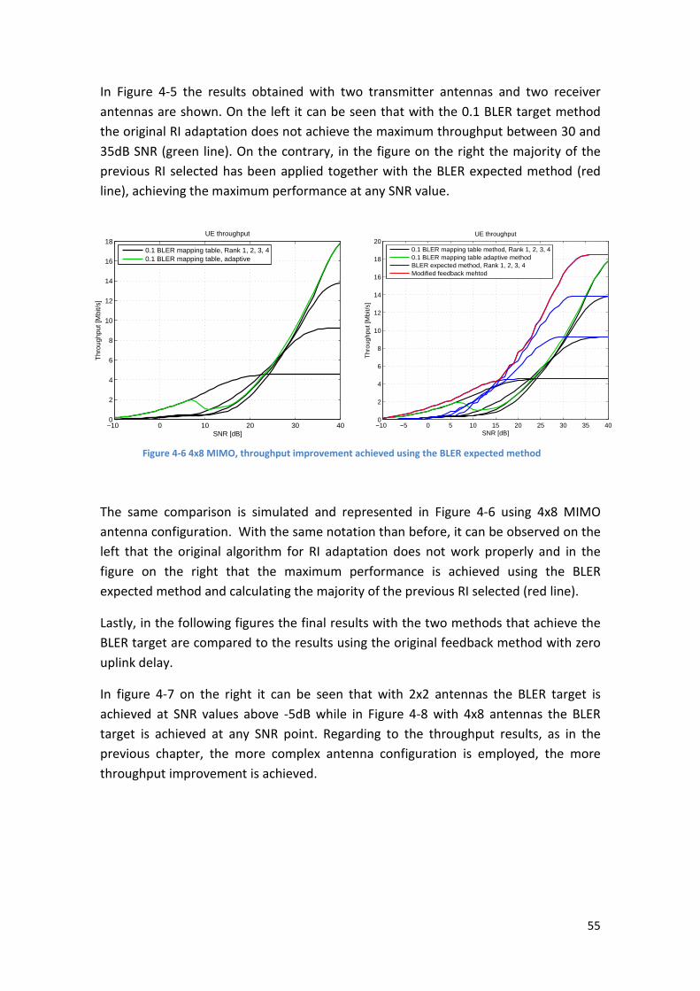
55

−10 0 10 20 30 400

2

4

6

8

10

12

14

16

18

SNR [dB]

Thr

ough

put [

Mbi

t/s]

UE throughput

0.1 BLER mapping table, Rank 1, 2, 3, 40.1 BLER mapping table, adaptive

−10 −5 0 5 10 15 20 25 30 35 400

2

4

6

8

10

12

14

16

18

20

SNR [dB]

Thr

ough

put [

Mbi

t/s]

UE throughput

0.1 BLER mapping table method, Rank 1, 2, 3, 40.1 BLER mapping table adaptive methodBLER expected method, Rank 1, 2, 3, 4Modified feedback mehtod

In Figure 4-5 the results obtained with two transmitter antennas and two receiver

antennas are shown. On the left it can be seen that with the 0.1 BLER target method

the original RI adaptation does not achieve the maximum throughput between 30 and

35dB SNR (green line). On the contrary, in the figure on the right the majority of the

previous RI selected has been applied together with the BLER expected method (red

line), achieving the maximum performance at any SNR value.

Figure 4-6 4x8 MIMO, throughput improvement achieved using the BLER expected method

The same comparison is simulated and represented in Figure 4-6 using 4x8 MIMO

antenna configuration. With the same notation than before, it can be observed on the

left that the original algorithm for RI adaptation does not work properly and in the

figure on the right that the maximum performance is achieved using the BLER

expected method and calculating the majority of the previous RI selected (red line).

Lastly, in the following figures the final results with the two methods that achieve the

BLER target are compared to the results using the original feedback method with zero

uplink delay.

In figure 4-7 on the right it can be seen that with 2x2 antennas the BLER target is

achieved at SNR values above -5dB while in Figure 4-8 with 4x8 antennas the BLER

target is achieved at any SNR point. Regarding to the throughput results, as in the

previous chapter, the more complex antenna configuration is employed, the more

throughput improvement is achieved.

56

−10 0 10 20 30 400

1

2

3

4

5

6

7

8

9

10

SNR [dB]

Thr

ough

put [

Mbi

t/s]

UE throughput

Zero uplink delay, Original feedback method10ms uplink delay, 0.1 BLER mapping table10ms uplink delay, Modified feedback method

−10 0 10 20 30 4010

−3

10−2

10−1

100

SNR [dB]

BLE

R

UE BLER

Zero uplink delay, Original feedback method10ms uplink delay, 0.1 BLER mapping table10ms uplink delay, Modified feedback method

−10 −5 0 5 10 15 20 25 30 35 400

2

4

6

8

10

12

14

16

18

20

SNR [dB]

Thr

ough

put [

Mbi

t/s]

UE throughput

Zero uplink delay, Original feedback method10ms uplink delay, 0.1 BLER mapping table10ms uplink delay, Modified feedback method

−10 0 10 20 30 4010

−3

10−2

10−1

100

SNR [dB]

BLE

R

UE BLER

Zero uplink delay, Original feedback method10ms uplink delay, 0.1 BLER mapping table10ms uplink delay, Modified feedback method

Figure 4-7 2x2 MIMO, final results that achieve the BLER target

Figure 4-8 4x8 MIMO, Final results that achieve the BLER target

4.3 Frequency-selective channel with multiple users

In this section the last investigation is explained. With the aim of studying the

performance obtained using the new feedback algorithms when several users are

placed in the same scenario, a frequency-selective channel with the simulations

parameters in table 2-8 is applied. In addition to these parameters, different

combinations of CQI and PMI granularity are simulated, specifically the four possible

combinations of granularity one and six.

57

Figure 4-9 Cell throughput improvement with BLER expected method

The solid lines in Figure 4-9 represent the results obtained with the four different

granularity configurations and using the original feedback method. When the

normalized Doppler frequency is below 0.1 the highest performance is achieved by

estimating a different CQI and PMI for each subband because the temporal correlation

is profound and the channel coherence time is not severe. Nevertheless, when the

normalized Doppler frequency increases above 0.1 the highest performance is

obtained by estimating a common PMI for all the available RBs because the correlation

decreases.

The red line with circles represents the result of applying again the BLER expected

method with CQI granularity one but in this case with adaptative PMI (granularity six).

The throughput obtained is higher than with fixed PMI, however, it can be seen in

Figure 4-10 that the BLER target is not achieved above 0.1 normalized Doppler

frequency. This happens because the PMI selected has been calculated under specific

channel conditions that have changed in the moment it is applied.

Finally, the red and blue lines with crosses correspond to the results obtained using the

BLER expected method with CQI granularity one and six, respectively, and both with

fixed PMI. These results are very similar in terms of throughput (Figure 4-9). With

regard to the BLER (Figure 4-10), when the CQI granularity is six the BLER values are

10−2

10−1

100

0

1

2

3

4

5

6

7

8

9

Normalized Doppler Frequency

Thr

ough

put [

Mbi

t/s]

Cell throughput

CQI 1, PMI 1CQI 1, PMI 6CQI 6, PMI 1CQI 6, PMI 6CQI 1, PMI 6, 0.1 BLER expectedCQI 1, fixed precoder, 0.1 BLER expectedCQI 6, fixed precoder, 0.1 BLER expected

58

close to 0.1, however, above this point. This is because an average CQI has been

estimated over all the RBs, which are assigned to different users, therefore if some

user is exposed to worst channel conditions it will not achieve the target with the CQI

estimated by averaging the channel conditions. The BLER target is only achieved at any

normalized Doppler frequency with CQI granularity one and fixed PMI.

Figure 4-10 Cell BLER improvement with BLER expected method

10−2

10−1

100

0

1

2

3

4

5

6

7

8

9

Normalized Doppler Frequency

Thr

ough

put [

Mbi

t/s]

Cell throughput

CQI 1, PMI 1CQI 1, PMI 6CQI 6, PMI 1CQI 6, PMI 6CQI 1, PMI6, Expected BLER methodCQI 1, fixed precoder, Expected BLER methodCQI 6, fixed precoder, Expected BLER method

59

60

5. CONCLUSIONS AND FUTURE RESEARCH

During the development of this thesis has been proved by simulations in different

scenarios that the user performance in terms of throughput and BLER decrease

considerably with the user velocity.

The two objectives considered at the beginning of these report are satisfied through

the implementation of new feedback algorithms that consider the channel statistics to

calculate the feedback indicators. The first objective is the improvement of the

throughput obtained by the user without considering that the BLER values are above

10% in most of the cases, and the second objective is the compliance of BLER results

without exceeding 10% due to this is the highest working point recommended in

wireless communications.

When it comes to interpreting the results presented, the fact that the HARQ process

could not be applied should be taken into account. In practice, it is expected a BLER

target fulfilment.

Regarding the study of the CQI, during which a SISO antenna configuration has been

employed, it can be concluded:

- The methods designed to improve the throughput achieve an important

improvement from 0.1 normalized Doppler frequency (corresponds to 50km/h

with 1ms uplink delay and 2.1GHz frequency carrier). In addition, the BLER

results are substantially lower compared to the BLER results using the original

algorithm, nevertheless above 10%.

- The BLER expected method achieves BLER<0.1 at any normalized Doppler

frequency point, however, this method implies a loss in throughput compared

to the results using the original feedback method.

With respect to the RI and PMI investigation, during which a MIMO antenna

configuration has been utilized, the main conclusions are:

- An increased throughput improvement and a decreased BLER values have been

observed when using more and more complex antenna configurations.

- In channels with considerably weak temporal correlation a fixed PMI offers

better results.

61

Lastly, through evaluating the proposed methods in a time and frequency selective

channel with multiple users it has been proved that:

- Once again the performance using the methods developed to improve the

throughput achieve gain with respect to the original feedback method when

the normalized frequency Doppler is above 0.1, reaching the same throughput

and BLER values irrespective of the CQI and PMI granularity with normalized

Doppler frequency above 0.25.

- The BLER expected method achieves the BLER target exclusively with CQI

granularity equal to one (different CQI value calculate for each RB/user) and a

fixed PMI value.

Even though the simulations have been performed using different antenna

configurations, different channel models and other different simulation parameters,

future research that could give us interesting results can be performed,

1. Results validation by applying the HARQ process. The 10% BLER boundary

should be accomplished with all the methods proposed and in any simulated

scenario.

2. Transmission mode 3 (OSLM) application, which is the most widely used at very

high velocity. This transmission mode is explained in section 2.2.2. Basically it

does not rely on any precoding matrix recommended by the user, using a fixed

precoding matrix defined by the standard. Furthermore, the diversity is

increased by incorporating Cyclic Delay Diversity.

3. Simulation of a non-perfect channel estimation. With the implementation of a

different channel estimation that introduces errors, the simulations would be

more realistic and a performance loss with the velocity with respect to the

results presented in this thesis would be observed.

4. Evaluation of the new feedback methods over MU-MIMO where the users are

spatially multiplexed. An important improvement is not expected using this

configuration because when the user velocity is considerably high the use of a

higher number of antennas in the transmitted than in the receiver is

recommended in order to obtain high user performance.

62

References

[1] JC Ikuno, C Mehlführer and M Rupp, “A novel link error prediction model for OFDM

systems with HARQ” Proc. IEEE International Conference on Communications (ICC

2011), Kyoto, Japan, 2011

[2] Starsky H.Y. Wong, Hao Yang, Songwu Lu and Vaduvur Bharghavan, ”Robust Rate

Adaptation for 802.11 Wireless Networks”, 2006

[3] Pravin Shankar, Tamer Nadeem, Justinian Rosca and Liviu Iftode “CARS: Context-

Aware Rate Selection for Vehicular Networks”, IEEE 2008

[4] Technical Specification Group Radio Access Network, “E-UTRA; physical channels

and modulation,” 3GPP, Tech. Rep. TS 36.211 Version 8.7.0, May 2009.

[5] S. Caban, C. Mehlführer, M. Rupp and M. Wrulich, “Evaluation of HDSPA and LTE:

From Testbed Measurements to System Level Performance”, 2011.

[6] Stefan Schwarz, Christian Mehlführer and Markus Rupp, “Calculation of the Spatial

Preprocessing and Link Adaption Feedback for 3GPP UMTS/LTE”, in Proc. IEEE Wireless

Advanced 2010, London, UK, 2010.

[7] Stefan Schwarz and Markus Rupp, “Throughput maximizing feedback for MIMO

OFDM based wireless communication systems”, in Proc. Signal Processing Advances in

Wireless Communications (SPAWC), 2011 San Francisco, CA.

[8] Erik Dahlman, Stefan Parkvall, and Johan Sköld “4G LTE/LTE-Advancedfor Mobile

Broadband”, 2011

[9] Ramón Agusti, Francisco Bernardo, Fernando Casadevall, Ramon Ferrús, Jordi

Pérez-Romero, Oriol Sallent, “LTE: nuevas tendencias en comunicaciones móviles”,

2010.

[10] M. J. Gans, “A power-spectral theory of propagation in the mobile-radio

environment,” IEEE Trans. Veh. Technol., vol. VT-21, pp. 27–38, Feb. 1972.

[11] R. H. Clarke, “A statistical theory of mobile-radio reception,” Bell Syst. Tech. J., pp.

957–1000, Jul.–Aug. 1968.

[12] C. Mehlführer, J. C. Ikuno, M. Šimko, S. Schwarz, M. Wrulich, and M. Rupp, “The

Vienna LTE simulators – Enabling Reproducibility in Wireless Communications

Research”, EURASIP Journal on Advances in Signal Processing, 2011.

[13] S. Schwarz, J. C. Ikuno, M. Šimko, M. Taranetz, Qi Wang and M. Rupp, “Pushing

the Limits of LTE: A Survey on Research Enhancing the Standard”, IEEE Access, 2013.

63

[14] Hassaan Touheed, Atta Ul Quddus and Rahim Tafazolli, “An Improved Link

Adaptation Scheme for High Speed Downlink Packet Access”, Vehicular Technology

Conference, 2008. VTC Spring 2008. IEEE, Singapore.

[15] S. Schwarz, M. Wrulich, and M. Rupp, “Mutual Information based Calculation of

the Precoding Matrix Indicator for 3GPP UMTS/LTE”, in Proc. IEEE Workshop on Smart

Antennas 2010, Bremen, Germany.

[16] Stefan Schwarz, Christian Mehlführer and Markus Rupp, “Throughput Maximizing

Multiuser Scheduling with Adjustable Fairness”, IEEE International Conference on

Communications (ICC), 2011, Kyoto.

[17] http://www.4gamericas.org/index.cfm?fuseaction=page&sectionid=272. Última

visita a la web, Noviembre de 2014.

[18] White Paper, “Architectural Considerations for Backhaul of 2G/3G and Long Term

Evolution Networks”. Disponible en

http://www.cisco.com/c/en/us/solutions/collateral/service-provider/mobile-

internet/white_paper_c11-613002.html. Última visita a la web, Noviembre de 2014

[19] White paper, “Doppler Spread and Coherence Time”. Disponible en

http://www.ni.com/white-paper/14911/en/. Última visita a la web, Noviembre de

2014.

64