Diploma in Statistics Introduction to Regression Lecture 3.11 Lecture 3.1 Multiple Regression...
60
Diploma in Statistics Introduction to Regression Lecture 3.1 1 Lecture 3.1 Multiple Regression (continued) • Review Homework • Review Analysis of Variance • Review model fitting and testing procedure • Case study: Predicting stamp sales for An Post – Problem formulation – Initial data analysis – Fitting and checking – Application
-
Upload
godwin-andrews -
Category
Documents
-
view
216 -
download
0
Transcript of Diploma in Statistics Introduction to Regression Lecture 3.11 Lecture 3.1 Multiple Regression...

Diploma in StatisticsIntroduction to Regression
Lecture 3.1 1
Lecture 3.1Multiple Regression (continued)
• Review Homework
• Review Analysis of Variance
• Review model fitting and testing procedure
• Case study: Predicting stamp sales for An Post
– Problem formulation
– Initial data analysis
– Fitting and checking
– Application

Diploma in StatisticsIntroduction to Regression
Lecture 3.1 2
Homework 2.2.1
Extend table of predictions of small medium and large jobs to include predictions based on the final fit. Compare and contrast.
Small Medium Large Original 155 447 969 Normal Revised 138 447 975 Final 140 445 965 Original 130 422 944 Rushed Revised 100 409 937 Final 102 407 927

Diploma in StatisticsIntroduction to Regression
Lecture 3.1 3
Homework 2.2.2
You have been asked to comment, as a statistical consultant, on a prediction formula for forecasting job completion times prepared by a former employee. The formula is, effectively, the one derived from the first fit discussed above. Write a report for management. Your report should refer to
(i) the practical usefulness of the employee's prediction formula, from a customer's perspective,
(ii) the significance of the exceptional cases from the customer's and management's perspectives, and
(iii) your recommended formula, with its relative advantages.

Diploma in StatisticsIntroduction to Regression
Lecture 3.1 4
Outline solution
(i) This formula is biased upwards for small jobs and downwards for large jobs.
Also, the prediction error associated with this prediction formula is ±75 hours, that is, ± 2 working weeks.
This means that we can predict the delivery time to be anywhere in a 4 week period. This is unlikely to be acceptable to our customers who have to meet exacting scheduling requirements of their own.

Diploma in StatisticsIntroduction to Regression
Lecture 3.1 5
Outline solution
(ii) There was one small job which took an excessively long time to complete. The causes for this need to be established with a view to preventing their recurrence.
The two longest jobs were subject to excessive variability, one taking an excessively long time and the other taking a remarkably short time. Again, the causes for these need to be established, with a view to reducing variability.
In the meantime, while the recommended prediction formula (see next) may be used with caution for long jobs, the prediction error is not valid for jobs longer than around 600 hours. Further experience with longer jobs is needed to establish a valid prediction formula.
Diploma in StatisticsIntroduction to Regression
Lecture 3.1 6
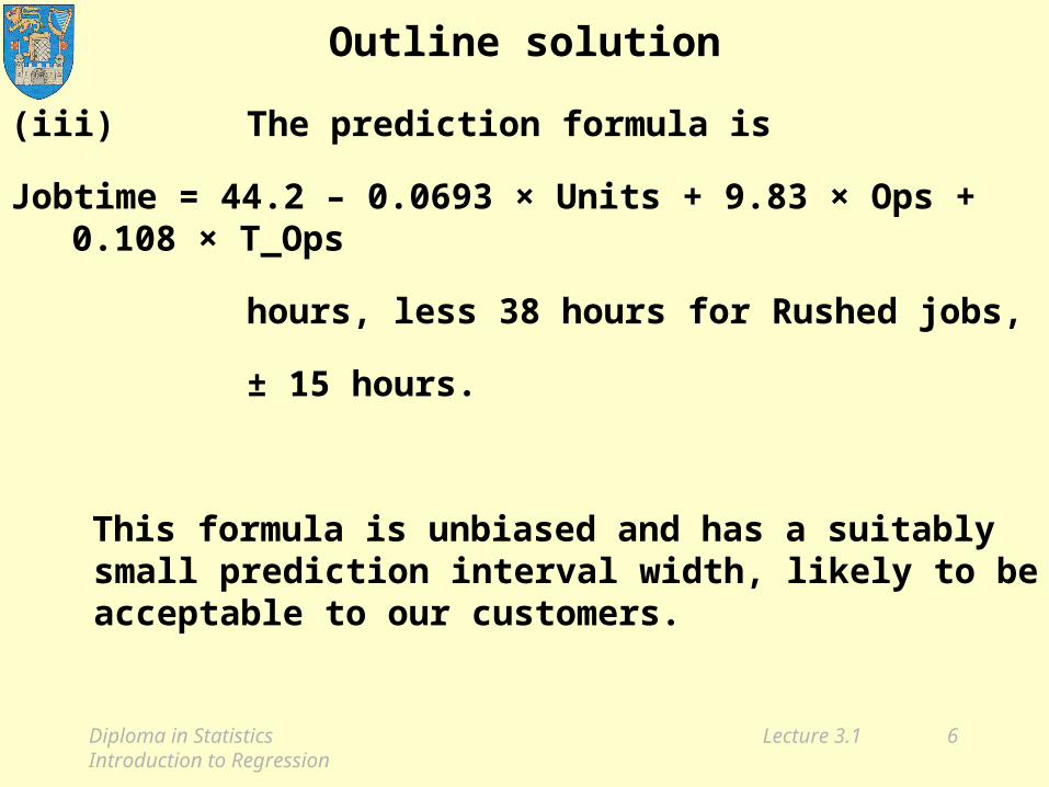
Outline solution
(iii) The prediction formula is
Jobtime = 44.2 – 0.0693 × Units + 9.83 × Ops + 0.108 × T_Ops
hours, less 38 hours for Rushed jobs,
± 15 hours.
This formula is unbiased and has a suitably small prediction interval width, likely to be acceptable to our customers.

Diploma in StatisticsIntroduction to Regression
Lecture 3.1 7
Homework 2.2.3
Make a table of the t values and corresponding s values for the three regressions
Compare, contrast and explain.

Diploma in StatisticsIntroduction to Regression
Lecture 3.1 8
Lecture 3.1Multiple Regression (continued)
• Review Homework
• Review Analysis of Variance
• Review model fitting and testing procedure
• Case study: Predicting stamp sales for An Post
– Problem formulation
– Initial data analysis
– Fitting and checking
– Application

Diploma in StatisticsIntroduction to Regression
Lecture 3.1 9
Analysis of Variance
S = 7.41272 R-Sq = 99.8% R-Sq(adj) = 99.7%
Analysis of Variance
Source DF SS MS F PRegression 4 299165 74791 1361.12 0.000Residual Error 12 659 55Total 16 299824
Residual Mean Square = s2: check!

Diploma in StatisticsIntroduction to Regression
Lecture 3.1 10
Analysis of Variance
Regression Sum of Squares measuresexplained variation
Residual Sum of Squares measuresunexplained (chance) variation
Total Variation = Explained + Unexplained
Coefficient of Determination:
Check it!
%Total
ExplainedR2

Diploma in StatisticsIntroduction to Regression
Lecture 3.1 11
Analysis of Variance
Regression Sum of Squares measuresexplained variation
Residual Sum of Squares measuresunexplained (chance) variation
Total Variation = Explained + Unexplained
F = MS(Reg) / MS(Res)
with 4 and 12 degrees of freedom.
Check it! Check F tables.

Diploma in StatisticsIntroduction to Regression
Lecture 3.1 12
Analysis of VarianceSelected 5% critical values for the F distribution
with 1 numerator and 2 denominator degrees of freedom
1 2 3 4 5 6 7 8 10 12 24 ∞
1 161.4 199.5 215.7 224.6 230.2 234.0 236.8 238.9 241.9 243.9 249.1 254.3 2 18.5 19.0 19.2 19.2 19.3 19.3 19.4 19.4 19.4 19.4 19.5 19.5 3 10.1 9.6 9.3 9.1 9.0 8.9 8.9 8.8 8.8 8.7 8.6 8.5 4 7.7 6.9 6.6 6.4 6.3 6.2 6.1 6.0 6.0 5.9 5.8 5.6 5 6.6 5.8 5.4 5.2 5.1 5.0 4.9 4.8 4.7 4.7 4.5 4.4 6 6.0 5.1 4.8 4.5 4.4 4.3 4.2 4.1 4.1 4.0 3.8 3.7 7 5.6 4.7 4.3 4.1 4.0 3.9 3.8 3.7 3.6 3.6 3.4 3.2 8 5.3 4.5 4.1 3.8 3.7 3.6 3.5 3.4 3.3 3.3 3.1 2.9 9 5.1 4.3 3.9 3.6 3.5 3.4 3.3 3.2 3.1 3.1 2.9 2.7
10 5.0 4.1 3.7 3.5 3.3 3.2 3.1 3.1 3.0 2.9 2.7 2.5 12 4.7 3.9 3.5 3.3 3.1 3.0 2.9 2.8 2.8 2.7 2.5 2.3 15 4.5 3.7 3.3 3.1 2.9 2.8 2.7 2.6 2.5 2.5 2.3 2.1 20 4.4 3.5 3.1 2.9 2.7 2.6 2.5 2.4 2.3 2.3 2.1 1.8 30 4.2 3.3 2.9 2.7 2.5 2.4 2.3 2.3 2.2 2.1 1.9 1.6 40 4.1 3.2 2.8 2.6 2.4 2.3 2.2 2.2 2.1 2.0 1.8 1.5
120 3.9 3.1 2.7 2.4 2.3 2.2 2.1 2.0 1.9 1.8 1.6 1.3
Diploma in StatisticsIntroduction to Regression
Lecture 3.1 13
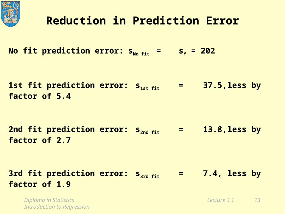
Reduction in Prediction Error
No fit prediction error: sNo fit = sY = 202
1st fit prediction error: s1st fit = 37.5, less by factor of 5.4
2nd fit prediction error: s2nd fit = 13.8, less by factor of 2.7
3rd fit prediction error: s3rd fit = 7.4, less by factor of 1.9

Diploma in StatisticsIntroduction to Regression
Lecture 3.1 14
Lecture 3.1Multiple Regression (continued)
• Review Homework
• Review Analysis of Variance
• Review model fitting and testing procedure
• Case study: Predicting stamp sales for An Post
– Problem formulation
– Initial data analysis
– Fitting and checking
– Application

Diploma in StatisticsIntroduction to Regression
Lecture 3.1 15
Step 1: Initial data analysis
• standard single variable summaries
– to determine extent of variation
– possible exceptional values;
• scatter plot matrix
– to view pair wise relationships between the response and the explanatory variables
and– to view pair wise relationships between the
explanatory variables themselves.

Diploma in StatisticsIntroduction to Regression
Lecture 3.1 16
Step 2: Least squares fit and interpretation
• calculate the best fitting regression coefficients
– check meaningfulness and statistical significance;
• calculate s
– check its usefulness for prediction
– its usefulness relative to alternative estimates of standard deviation.

Diploma in StatisticsIntroduction to Regression
Lecture 3.1 17
Step 3: Diagnostic analysis of residuals
• diagnostic plot
– check for exceptional residuals or patterns of residuals,
– possible explanations in terms of the fitted values;
• Normal plot
– check for exceptional residuals or non-linear patterns in the residuals

Diploma in StatisticsIntroduction to Regression
Lecture 3.1 18
Step 4: Iterate fit and check
• determine cases for deletion
– repeat steps 2 and 3 until checks are passed.

Diploma in StatisticsIntroduction to Regression
Lecture 3.1 19
Lecture 3.1Multiple Regression (continued)
• Review Homework
• Review Analysis of Variance
• Review model fitting and testing procedure
• Case study: Predicting stamp sales for An Post
– Problem formulation
– Initial data analysis
– Fitting and checking
– Application

Diploma in StatisticsIntroduction to Regression
Lecture 3.1 20
The Stamp Sales Case Study
The problem
• January 1984, An Post established
• New business plan; sales forecasts required
• Historical sales data available

Diploma in StatisticsIntroduction to Regression
Lecture 3.1 21
Historical dataTable 1.4 Annual sales of stamps and metered mail, 1949 - 1983
Year Stamp Sales1
Meter Sales
Total Sales
Year Stamp Sales
Meter Sales
Total Sales
1949 245.2 42.0 287.2 1967 234.3 162.8 397.1 1950 224.4 48.6 273.0 1968 238.6 169.3 407.9 1951 241.3 52.1 293.4 1969 242.7 186.5 429.3 1952 251.3 60.9 312.3 1970 226.4 197.5 423.9 1953 236.7 65.8 302.5 1971 199.4 172.2 371.6 1954 231.6 69.1 300.7 1972 205.4 192.8 398.2 1955 235.8 75.1 310.8 1973 201.6 195.9 397.4 1956 253.0 90.4 343.4 1974 191.1 199.6 390.8 1957 262.6 98.1 360.7 1975 181.0 213.3 394.3 1958 265.4 104.6 370.0 1976 174.9 240.9 415.8 1959 266.0 107.5 373.4 1977 181.0 258.4 439.3 1960 278.4 112.4 390.8 1978 188.2 240.8 429.0 1961 277.7 116.9 394.6 1979 112.5 163.5 276.0 1962 235.9 105.0 340.9 1980 163.7 211.5 375.2 1963 230.0 105.2 335.2 1981 162.1 195.3 357.4 1964 234.8 121.3 356.1 1982 148.9 228.5 377.4 1965 228.8 149.0 377.8 1983 151.2 259.7 410.9 1966 230.1 153.7 383.8 1 Sales are recorded as millions of standard stamp equivalents, that is, total revenue in a year divided by
the price of a stamp for a standard sealed letter for internal delivery, and divided by 1,000,000.

Diploma in StatisticsIntroduction to Regression
Lecture 3.1 22
Trend projection?
Hire a consultant!
100
200
300
400
Data
1950 1960 1970 1980
Year
Stamp Sales
Meter Sales
Total Sales

Diploma in StatisticsIntroduction to Regression
Lecture 3.1 23
Factors influencing sales
• Economic growth
• Stamp prices
• Alternative product prices
measurement problems!

Diploma in StatisticsIntroduction to Regression
Lecture 3.1 24
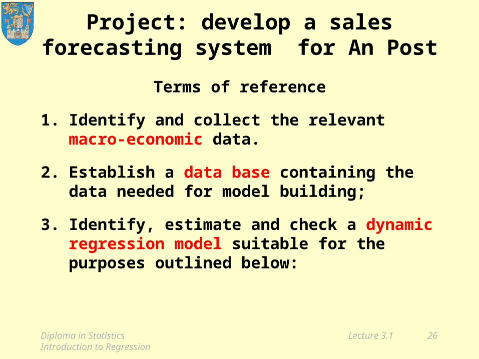
Project: develop a sales forecasting system for An Post
Terms of reference
1. Identify and collect the relevant macro-economic data.
2. Establish a data base containing the data needed for model building;
3. Identify, estimate and check a dynamic regression model suitable for the purposes outlined below:

Diploma in StatisticsIntroduction to Regression
Lecture 3.1 25
(a) medium-term (one to five years) forecasting of aggregate demand for postal services;
(b) analysis of the effects of levels of general economic activity, postal prices and the prices of competing services, on aggregate demand for postal services;
(c) use as a benchmark for the analysis of the effects of demand stimulation activities.
Diploma in StatisticsIntroduction to Regression
Lecture 3.1 26
Project: develop a sales forecasting system for An Post
Terms of reference
1. Identify and collect the relevant macro-economic data.
2. Establish a data base containing the data needed for model building;
3. Identify, estimate and check a dynamic regression model suitable for the purposes outlined below:

Diploma in StatisticsIntroduction to Regression
Lecture 3.1 27
(a) medium-term (one to five years) forecasting of aggregate demand for postal services;
(b) analysis of the effects of levels of general economic activity, postal prices and the prices of competing services, on aggregate demand for postal services;
(c) use as a benchmark for the analysis of the effects of demand stimulation activities.

Diploma in StatisticsIntroduction to Regression
Lecture 3.1 28
Explanatory variables
• General economic activity:
– Gross National Product GNP
• Postal prices:
– Real Letter Price RLP
• Prices of competing services:
– Real Phone Charge RPC

Diploma in StatisticsIntroduction to Regression
Lecture 3.1 29
Definitions
• GNP measures the value of all goods and services produced by all residents of the state

Diploma in StatisticsIntroduction to Regression
Lecture 3.1 30
Definitions
Real Letter Price:
• the price of a standard sealed internal letter
divided by
• the Consumer Price Index (CPI);
measures relative change in the price of a stamp,
relative to changes in the prices of other goods and services

Diploma in StatisticsIntroduction to Regression
Lecture 3.1 31
Definitions
• Real Phone Charge:
the price of a local telephone call
divided by the
Consumer Price Index (CPI)

Diploma in StatisticsIntroduction to Regression
Lecture 3.1 32
Table 8.7 Annual postage stamp sales, GNP,real letter prices and real phone charges, 1949-1983
Year Stamp Sales
GNP RLP1 RPC2 Year Stamp Sales
GNP RLP1 RPC2
1949 245.2 552.6 1.047 0.419 1967 234.3 848.4 1.090 0.654 1950 224.4 557.0 1.031 0.413 1968 238.6 919.4 1.040 0.624 1951 241.3 564.3 0.957 0.383 1969 242.7 970.7 1.164 0.582 1952 251.3 580.1 0.880 0.352 1970 226.4 1002.6 1.206 0.714 1953 236.7 598.1 0.946 0.501 1971 199.4 1037.3 1.570 0.655 1954 231.6 603.9 0.998 0.499 1972 205.4 1112.5 1.453 0.603 1955 235.8 616.0 0.974 0.487 1973 201.6 1154.5 1.464 0.541 1956 253.0 608.3 0.934 0.622 1974 191.1 1201.7 1.526 0.557 1957 262.6 611.8 0.897 0.598 1975 181.0 1223.5 1.616 0.544 1958 265.4 600.9 0.859 0.572 1976 174.9 1229.7 1.764 0.626 1959 266.0 626.6 0.859 0.572 1977 181.0 1316.2 1.677 0.551 1960 278.4 658.9 0.855 0.570 1978 188.2 1388.4 1.598 0.639 1961 277.7 690.9 0.832 0.554 1979 112.5 1422.8 1.526 0.564 1962 235.9 716.0 0.997 0.532 1980 163.7 1462.2 1.607 0.577 1963 230.0 749.6 1.039 0.519 1981 162.1 1492.6 1.835 0.580 1964 234.8 780.7 1.113 0.730 1982 148.9 1473.2 2.114 0.601 1965 228.8 800.7 1.158 0.695 1983 151.2 1462.6 1.993 0.651 1966 230.1 806.8 1.124 0.675
1 The Real Letter Price (RLP) is the price of a standard sealed internal letter divided by the Consumer Price Index.
2 The Real Phone Charge (RPC) is the price of a local telephone call divided by the Consumer Price Index.

Diploma in StatisticsIntroduction to Regression
Lecture 3.1 33
Prediction model?Multiple linear regression
How are Stamps Sale (Y) related to
• Gross National Product (GNP = X1 ),
• Real Letter Price (RLP = X2 ),
• Real Phone Charge (RPC = X3 ) ?
Try
332211 XXXY

Diploma in StatisticsIntroduction to Regression
Lecture 3.1 34
Example
Best prediction equation:
• Predicted Sales = 343 – .0577 GNP – 53.2 RLP
• To calculate the predicted sales for any year, find the values of GNP and RLP for that year and substitute them in the equation.
Application
Evaluate the effect on sales of the industrial action in 1979.
Actual sales (1979): 112.5GNP(1979): 1,422.8RLP(1979): 1.526

Diploma in StatisticsIntroduction to Regression
Lecture 3.1 35
Application
Evaluate the effect on sales of the industrial action in 1979.
Actual sales (1979): 112.5GNP(1979): 1,422.8RLP(1979): 1.526
"Predicted" Sales:
343 – .0577 GNP – 53.2 RLP
= 343 – .0577 × 1422.8 – 53.2 × 1.526
= 179.7
Effect = 112.5 – 179.7 = – 67.2
Diploma in StatisticsIntroduction to Regression
Lecture 3.1 36
Lecture 3.1Multiple Regression (continued)
• Review Homework
• Review Analysis of Variance
• Review model fitting and testing procedure
• Case study: Predicting stamp sales for An Post
– Problem formulation
– Initial data analysis
– Fitting and checking
– Application

Diploma in StatisticsIntroduction to Regression
Lecture 3.1 37
Step 1: Initial data analysis, dotplots

Diploma in StatisticsIntroduction to Regression
Lecture 3.1 38
Initial data analysis, time plots
1950 1960 1970 1980
Year
100
150
200
250
300
Stamp Sales
1950 1960 1970 1980
Year
600
800
1000
1200
1400
GNP
1950 1960 1970 1980
Year
1.0
1.2
1.4
1.6
1.8
2.0
RLP
1950 1960 1970 1980
Year
0.4
0.5
0.6
0.7
RPC

Diploma in StatisticsIntroduction to Regression
Lecture 3.1 39
Initial data analysis, scatterplot matrix

Diploma in StatisticsIntroduction to Regression
Lecture 3.1 40
Initial data analysis, scatterplot matrix

Diploma in StatisticsIntroduction to Regression
Lecture 3.1 41
Initial data analysis, scatterplot matrix

Diploma in StatisticsIntroduction to Regression
Lecture 3.1 42
Lecture 3.1Multiple Regression (continued)
• Review Homework
• Review Analysis of Variance
• Review model fitting and testing procedure
• Case study: Predicting stamp sales for An Post
– Problem formulation
– Initial data analysis
– Fitting and checking
– Application
Diploma in StatisticsIntroduction to Regression
Lecture 3.1 43
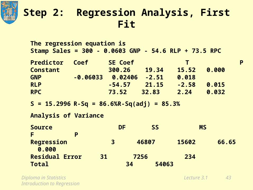
The regression equation isStamp Sales = 300 - 0.0603 GNP - 54.6 RLP + 73.5 RPC
Predictor Coef SE Coef T PConstant 300.26 19.34 15.52 0.000GNP -0.06033 0.02406 -2.51 0.018RLP -54.57 21.15 -2.58 0.015RPC 73.52 32.83 2.24 0.032
S = 15.2996 R-Sq = 86.6%R-Sq(adj) = 85.3%
Analysis of Variance
Source DF SS MS F PRegression 3 46807 15602 66.65 0.000Residual Error 31 7256 234Total 34 54063
Step 2: Regression Analysis, First Fit

Diploma in StatisticsIntroduction to Regression
Lecture 3.1 44
Exercise
Explain the Degrees of Freedom
Check the calculation of:
MS(Regression)
MS(Error)
s
R2
F
T
Check the statistical significance of the coefficients

Diploma in StatisticsIntroduction to Regression
Lecture 3.1 45
Step3: Diagnostic Analysis

Diploma in StatisticsIntroduction to Regression
Lecture 3.1 46
Step 4: Iterate the analysis, 1979 deleted
Predictor Coef SE Coef T PConstant 317.96 11.90 26.71 0.000GNP -0.00771 0.01614 -0.48 0.636RLP -92.18 13.72 -6.72 0.000RPC 43.29 20.21 2.14 0.040
S = 9.22460
Exercise:Compare s to previous value.
Compare coefficient estimates to previous values.

Diploma in StatisticsIntroduction to Regression
Lecture 3.1 47
Compare fits

Diploma in StatisticsIntroduction to Regression
Lecture 3.1 48
1980
Diagnostic plots, 1979 deleted
after1970
up to1970
Diploma in StatisticsIntroduction to Regression
Lecture 3.1 49
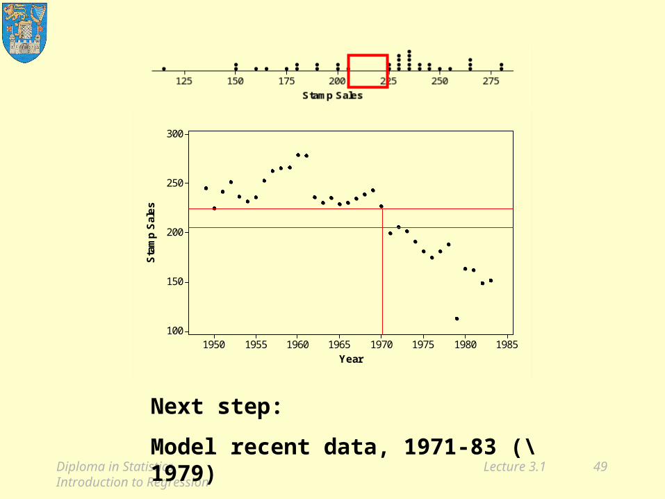
19851980197519701965196019551950
300
250
200
150
100
Year
Sta
mp
Sal
es
Next step:
Model recent data, 1971-83 (\1979)
Diploma in StatisticsIntroduction to Regression
Lecture 3.1 50
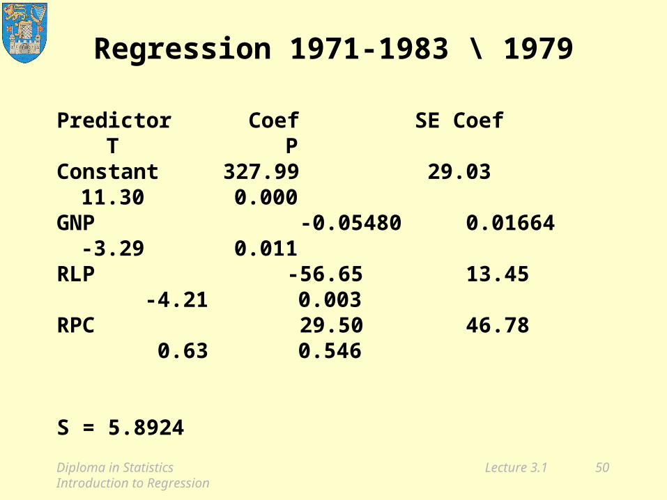
Regression 1971-1983 \ 1979
Predictor Coef SE Coef T PConstant 327.99 29.03 11.30 0.000GNP -0.05480 0.01664 -3.29 0.011RLP -56.65 13.45 -4.21 0.003RPC 29.50 46.78 0.63 0.546
S = 5.8924

Diploma in StatisticsIntroduction to Regression
Lecture 3.1 51
210200190180170160150140
3
2
1
0
-1
-2
-3
-4
Fitted Value
De
lete
d R
esi
du
alVersus Fits
(response is Stamp Sales)

Diploma in StatisticsIntroduction to Regression
Lecture 3.1 52
4
3
2
1
0
-1
-2
-3
-4210-1-2
De
lete
d R
esi
du
al
Score
N 12
AD 0.543
P-Value 0.128
Normal Probability Plot(response is Stamp Sales)

Diploma in StatisticsIntroduction to Regression
Lecture 3.1 53
Regression with 1980, RPC deleted
Predictor Coef SE Coef T PConstant 339.58 10.62 31.96 0.000GNP -0.03158 0.01329 -2.38 0.045RLP -70.155 9.660 -7.26 0.000
S = 3.92988 R-Sq = 96.8%

Diploma in StatisticsIntroduction to Regression
Lecture 3.1 54
Lecture 3.1Multiple Regression (continued)
• Review Homework
• Review Analysis of Variance
• Review model fitting and testing procedure
• Case study: Predicting stamp sales for An Post
– Problem formulation
– Initial data analysis
– Fitting and checking
– Application

Diploma in StatisticsIntroduction to Regression
Lecture 3.1 55
Exercise
Calculate the predicted stamp sales for 1984 and 1985. Assume no change in nominal stamp price.
Compare with the actual outcomes:
1984 1985
Sales 163.6 172.1
GNP 1487.5 1466.6
RLP 1.835 1.741
Comment on the prediction errors.

Diploma in StatisticsIntroduction to Regression
Lecture 3.1 56
Exercise
Predicted Sales = 300 – .0312 GNP – 70.155 RLP
To calculate the predicted sales for any year, find the values of GNP and RLP for that year and substitute them in the equation.
Problem: how to get GNP and RLP for future years?
Answer: use "official" predictions.

Diploma in StatisticsIntroduction to Regression
Lecture 3.1 57
Central Bank predictions for 1984, 1985
1984 1985GNP: + 1.5% + 1.5%Inflation: + 8.6% + 5.5%
NB: no change in nominal stamp price in 1984 or 1985
GNP(83) = 1462.6;predicted GNP(84) = 1462.6 × 1.015 = 1484.5
RLP(83) = 1.993;
assuming no change in nominal stamp price,
predicted RLP(84) = 1.993 / 1.086 = 1.835

Diploma in StatisticsIntroduction to Regression
Lecture 3.1 58
Prediction for 1984
GNP(84) = 1484.5
RLP(84) = 1.835
Predicted Sales = 340 – .0316 × GNP – 70.155 × RLP
= 340 – .0316 × 1484.5 – 70.155 × 1.835
= 164.4
Actual outcome: 163.6
Prediction for 1985? Homework 3.1.1

Diploma in StatisticsIntroduction to Regression
Lecture 3.1 59
Homework 3.1.2
Carry out the analysis of stamp sales data prior to 1970, leading to the prediction formula
Sales = 371 – 176 RLP + 84 RPC,
s = 5.5.
Compare early and recent prediction formulas, including prediction errors.
Ref:SA pp. 282-4

Diploma in StatisticsIntroduction to Regression
Lecture 3.1 60
Reading
SA § 1.6, §8.7
Alternative readings
Hamilton, Ch 2, up to p. 53,
Ch 3, pp. 65-72, 74-75, 77-80,
Ch 4, pp. 109-117