Dip 03 Management Accounting - OAsis Home
337
MANAGEMENT ACCOUNTING
Transcript of Dip 03 Management Accounting - OAsis Home

MANAGEMENT ACCOUNTING
Management Accounting Course Author: Dr. Dennis Caplan (Original OER Author – See Acknowledgement). Course Editor: Dr. Roger Powley Commonwealth of Learning Edition 1 ____________________
Commonwealth of Learning © 2012 Any part of this document may be reproduced without permission but with attribution to the Commonwealth of Learning using the CC‐BY‐SA (share alike with attribution). http://creativecommons.org/licenses/by‐sa/4.0
Commonwealth of Learning 4710 Kingsway, Suite 2500 Burnaby, British Columbia
Canada V5H 4M2 Telephone: +1 604 775 8200
Fax: +1 604 775 8210 Web: www.col.org
E‐mail: [email protected]
ACKNOWLEDGEMENTS
The Commonwealth of Learning wishes to attribute the content of this course to Dr.
Dennis Caplan of the University at Albany (State University of New York). The course in
its original form was an e‐course available at http://denniscaplan.fatcow.com/TOC.htm.
The online content was offered as an OER using the CC BY SA license. It has been re‐
purposed by the Commonwealth of Learning into a paper‐based course for use as a
foundation course in a Bachelor’s of Business and Entrepreneurship. Thanks to Dr.
Caplan.


Management Accounting Page | i
TABLE OF CONTENTS
COURSE OVERVIEW................................................................................................................................. 1
Introduction ........................................................................................................................................ 1
Course Goals ....................................................................................................................................... 1
Description .......................................................................................................................................... 1
Required Readings .............................................................................................................................. 1
Assignments and Projects ................................................................................................................... 1
Assessment Methods .......................................................................................................................... 1
Course Schedule .................................................................................................................................. 2
STUDENT SUPPORT ................................................................................................................................. 3
Academic Support ............................................................................................................................... 3
How to Submit Assignments ............................................................................................................... 3
Technical Support ............................................................................................................................... 3
UNIT 1 – INTRODUCTION TO MANAGEMENT ACCOUNTING ................................................................. 4
Unit Introduction ................................................................................................................................ 4
Unit Objectives .................................................................................................................................... 4
Unit Readings ...................................................................................................................................... 4
Assignments and Activities ................................................................................................................. 4
lesson 1.1: Management Accounting vs. Financial Accounting .......................................................... 5
Lesson 1.2: Concepts and History of Management Accounting ....................................................... 13
Unit 1 – Summary ............................................................................................................................. 21
UNIT 2: MICROECONOMIC FOUNDATIONS OF MANAGEMENT ACCOUNTING ................................... 22
Unit Introduction .............................................................................................................................. 22
Unit Objectives .................................................................................................................................. 22
Unit Readings .................................................................................................................................... 22
Assignments and Activities ............................................................................................................... 22
Lesson 2.1: Relevant Cost Analysis ................................................................................................... 23
LESSON 2.2: Cost Behaviour .............................................................................................................. 32
Lesson 2.3: Cost‐Volume‐Profit ........................................................................................................ 41
Lesson 2.4: Flexible Budgeting .......................................................................................................... 51
Lesson 2.5: Cost Variances for Direct Materials and Labour ............................................................ 62
Unit 2 – Summary ............................................................................................................................. 78
Page | ii Management Accounting
UNIT 3: PRODUCT COSTING AND COST ALLOCATIONS ......................................................................... 79
Unit Introduction .............................................................................................................................. 79
Unit Objectives .................................................................................................................................. 79
Unit Readings .................................................................................................................................... 79
Assignments and Activities ............................................................................................................... 79
Lesson 3.1: Product Costing .............................................................................................................. 80
Lesson 3.2: Normal Costing ............................................................................................................... 95
Lesson 3.3: Standard Costing .......................................................................................................... 108
Lesson 3.4: Activity‐Based Costing .................................................................................................. 124
Lesson 3.5: Allocation of Service Department Costs ...................................................................... 142
Lesson 3.6: The Role of Cost in Setting Prices ................................................................................. 156
Unit 3 – Summary ........................................................................................................................... 168
UNIT 4: DETERMINING THE COST OF INVENTORY .............................................................................. 169
Unit Introduction ............................................................................................................................ 169
Unit Objectives ................................................................................................................................ 169
Unit Readings .................................................................................................................................. 169
Assignments and Activities ............................................................................................................. 169
LESSON 4.1: Work‐in‐Process ......................................................................................................... 170
Lesson 4.2: Alternative Inventory Valuation Methods ................................................................... 181
LESSON 4.3: Fixed Manufacturing Overhead .................................................................................. 199
LESSON 4.4: Cost Variances for Variable and Fixed Overhead ....................................................... 211
Lesson 4.5: Joint Products ............................................................................................................... 228
Unit 4 – Summary ........................................................................................................................... 235
UNIT 5: PLANNING TOOLS AND PERFORMANCE MEASURES ............................................................. 236
Unit Introduction ............................................................................................................................ 236
Unit Objectives ................................................................................................................................ 236
Unit Readings .................................................................................................................................. 236
Assignments and Activities ............................................................................................................. 236
LESSON 5.1: Capital Budgeting........................................................................................................ 237
Lesson 5.2: Operating Budgets ....................................................................................................... 256
Lesson 5.3: Budgetary Incentive Schemes ...................................................................................... 272
Lesson 5.4: Divisional Performance Measures ............................................................................... 277
Lesson 5.6: Corporate Social Responsibility .................................................................................... 302
Unit 5 – Summary ........................................................................................................................... 313
Management Accounting Page | iii
Course Summary ................................................................................................................................. 314
GLOSSARY............................................................................................................................................ 320


Management Accounting Page | 1
COURSE OVERVIEW
INTRODUCTION
The Management Accounting course will prepare future entrepreneurs to effectively manage the resources, equipment, facilitates, finances and inventory of a business. We will explore costing systems, inventory control, facilities management and budget preparation and management.
COURSE GOALS
Upon completion of this course future entrepreneurs will be able to:
1. Employ costing systems to manage the business. 2. Employ activity based management tools and techniques. 3. Identify costing variables for analysis. 4. Prepare a annual budget and multi‐year budget. 5. Describe how to stay on budget. 6. Use cost and performance measures. 7. Conduct performance cost variance analysis. 8. Establish pricing models. 9. Manage inventories, equipment and resources. 10. Establish depreciation targets. 11. Produce and analyse quarterly and year end statements of account.
DESCRIPTION
This course consists of five units and a glossary. The units are:
Unit 1 – Introduction to Management Accounting.
Unit 2 – Microeconomic Foundations of Management Accounting.
Unit 3 – Product Costing and Cost Allocations.
Unit 4 – Determining the Cost of Inventory.
Unit 5 – Planning Tools and Performance Measures.
REQUIRED READINGS
To be identified by the instructor.
ASSIGNMENTS AND PROJECTS
This course includes lesson level exercises and problems that students are required to
complete before moving on to the next lesson or unit of instruction.
ASSESSMENT METHODS
You will be required create and maintain an Problems Workbook. Answers to the
problems presented at the end of each lesson must be recorded in the workbook. You

Page | 2 Management Accounting
instructor will regularly review your workbook, or ask that you submit portions of your
workbook for review and grading.
Your instructor will provide guidance on how he or she is going to grade the course and
the type of assignments or projects that must be submitted as you work through the
course materials.
COURSE SCHEDULE
This course is designed to fit into a twelve to fourteen week academic period. Your
instructor will provide a detailed schedule which reflects which units and lessons must
be completed each week and when the assignments or projects must be submitted for
review and feedback.

Management Accounting Page | 3
STUDENT SUPPORT
ACADEMIC SUPPORT
<Insert the following information if relevant>
How to contract a tutor/facilitator (Phone number, email, office hours, etc.).
Background information about the tutor/facilitator if he/she does not change
regularly. Alternatively provide a separate letter with the package describing
your tutor/facilitator’s background.
Description of any resources that they may need to procure to complete the
course (e.g. lab kits, etc.).
How to access the library (either in person, by email or online).
HOW TO SUBMIT ASSIGNMENTS
<If the course requires that assignments be regularly graded, then insert a description
of how and where to submit assignments. Also explain how the learners will receive
feedback.>
TECHNICAL SUPPORT
<If the students must access content online or use email to submit assignments, then a
technical support section is required. You need to include how to complete basic tasks
and a phone number that they can call if they are having difficulty getting online>.
Page | 4 Management Accounting
UNIT 1 – INTRODUCTION TO MANAGEMENT ACCOUNTING
UNIT INTRODUCTION
Management accounting or managerial accounting is concerned with the provisions
and use of accounting information by managers within organizations. The information
provides them with the facts needed to make informed business decisions.
Management accounting data allows them to be better equipped in their management
and control functions.
The new entrepreneur and the seasoned business professional must all be grounded in
the practice of management accounting techniques and methods. They must be able to
capture the data and they must be able to interpret it in a way that ensures effective
management of their organization.
This unit will explore the concepts underlying management accounting.
UNIT OBJECTIVES
Upon completion of this unit you will be able to:
1. Define management accounting.
2. Describe the history of management accounting.
3. Explain the concepts underlying management accounting.
4. Explain the similarities and differences between management accounting and
financial accounting.
UNIT READINGS
As you complete this unit you are required to read the following lessons/articles:
<To be provided by your instructor>.
ASSIGNMENTS AND ACTIVITIES
This unit of instruction has no assignments, activities or exercises to complete. Ensure
you complete any readings assigned by the instructor before proceeding to the next
unit of instruction.

Management Accounting Page | 5
LESSON 1.1: MANAGEMENT ACCOUNTING VS. FINANCIAL ACCOUNTING
LESSON INTRODUCTION
We all face the fundamental economic problem of how to allocate scarce resources.
This is a problem that confronts every company, every government, and us as a society.
It is a problem that we each face in our families and as individuals.
In the United States and throughout most of the world, there are institutions that
facilitate this allocation of scarce resources. The New York Stock Exchange is one such
institution, as is the London Stock Exchange, the Chicago Board of Trade, and all other
stock, bond and commodity markets. These financial markets are sophisticated and
apparently efficient mechanisms for channelling resources from investors to those
companies that investors believe will use those resources most profitably.
Banks and other lending institutions also allocate scarce resources across companies,
through their credit and lending decisions. Governments allocate scarce resources
across segments of society. They collect taxes from companies and individuals, and
allocate resources to achieve social and economic goals.
All of these institutions use financial accounting as a primary source of information for
these allocation decisions. Investors and stock analysts review corporate financial
statements prepared in accordance with Generally Accepted Accounting Principles.
Banks review financial statements as well as projections of cash flows and financial
performance. The Internal Revenue Service taxes income that is calculated only slightly
differently from income for financial reporting purposes. In effect, the same set of
financial accounting rules is used by these different users, with only minor
modifications.
However, this is only part of the story, because when I buy stock in Microsoft, whether
my investment turns out to be profitable depends largely on the operational, marketing
and strategic decisions that Microsoft’s managers make during the time that I hold my
investment. And when Microsoft’s management team sits down to decide what
products to develop, which markets to enter, and how to source production, they are
not, almost certainly, looking at the company’s most recent annual report or any other
financial accounting report. By the time the annual report is available, the information is
too old, and in any case, it is too highly summarized; there is not enough detail and not
enough forward‐looking data. Rather, when Microsoft’s management team makes
decisions, it bases these decisions on management accounting information. This is
definitional. By definition, management accounting is the information that managers
use for decision‐making. By definition, financial accounting is information provided to
external users.
Hence, both financial accounting and management accounting are all about allocating
scarce resources. Financial accounting is the principle source of information for
decisions of how to allocate resources among companies, and management accounting
is the principle source of information for decisions of how to allocate resources within a
company. Management accounting provides information that helps managers control

Page | 6 Management Accounting
activities within the firm, and to decide what products to sell, where to sell them, how
to source those products, and which managers to entrust with the company’s
resources.
* * * * * *
In other news, General Motors’ common stock rose $1.10 today following the
announcement that the company has successfully installed an improved
management accounting system.
* * * * * *
If management accounting so important, why are we not likely to see a headline like the
fictional announcement shown above? There are two reasons. First, management
accounting information is proprietary; public companies are generally not required to
disclose management accounting data nor much detail about the systems that generate
this information. Typically, companies disclose very little management accounting
information to investors and analysts beyond what is imbedded in financial reporting
requirements. Even very basic information, such as unit sales by major product
category, or product costs by product type, is seldom reported, and when it is reported
one can be sure that management believes voluntary disclosure of this information will
be viewed as “good news” by the marketplace.
The second reason we are not likely to see a headline like the one above is that most
management accounting systems seem to work reasonably well most of the time.
Hence, it is difficult for a company to gain a competitive advantage by installing a better
management accounting system than its competitors. However, this observation does
not imply that management accounting systems are not important. On the contrary, as
the following news story indicates, poor management accounting systems can
significantly affect the investment community’s perception of a company’s prospects.
NEW YORK TIMES
OCTOBER 28, 1997
Oxford Health Plans said yesterday that it had been losing money because
it fell behind in sending bills to customers and underestimated how much it
owed doctors and hospitals. Shares fell 62%. Stephen Wiggins, chairman of
Oxford, said the company had belatedly discovered that many customers
were not paying premiums, often because the company was late in sending
bills.
Oxford acknowledged that it had fallen behind in payments to hospitals
and doctors as it struggled with a new computer system. With incomplete
information in its computers, it had to advance money to doctors and
hospitals without verifying that they were obeying Oxford's rules. Mr
Wiggins said Oxford would add about 0.5% to spending on administration

Management Accounting Page | 7
next year in an effort to insure there are no similar problems. “The
important thing," he added, "is we're the same company we were on
Friday, except our market value has dropped by half.”
Health insurance is a relatively stable industry. 1997 was the middle of a strong bull
market. What was the problem with Oxford such that in this environment it should lose
half its stock value almost overnight? The answer is that its management accounting
system was broken, big time. Management accounting is something like indoor
plumbing. When it functions properly, we tend to take it for granted, but when it breaks
down, we quickly develop a greater appreciation for it.
LESSON OBJECTIVES
Upon completion of this lesson you will be able to:
1. Recognize the three types of accounting practices as financial accounting,
management accounting and auditing.
2. Describe the scope of management accounting.
3. Explain the differences between management accounting and financial
accounting.
SCOPE OF MANAGEMENT ACCOUNTING
Management accounting is the process of measuring and reporting information about
economic activity within organizations, for use by managers in planning, performance
evaluation, and operational control.
Planning: For example, deciding what products to make, and where and when to
make them. Determining the materials, labour, and other resources that are needed
to achieve desired output. In not‐for‐profit organizations, deciding which programs
to fund.
Performance Evaluation: Evaluating the profitability of individual products and
product lines. Determining the relative contribution of different managers and
different parts of the organization. In not‐for‐profit organizations, evaluating the
effectiveness of managers, departments and programs.
Operational Control: For example, knowing how much work‐in‐process is on the
factory floor, and at what stages of completion, to assist the line manager in
identifying bottlenecks and maintaining a smooth flow of production.
Also, the management accounting system usually feeds into the financial accounting
system. In particular, the product costing system is usually used to help determine
inventory balance sheet amounts, and the cost of sales for the income statement.
Management accounting information is usually financial in nature and dollar‐
denominated, although increasingly, management accounting systems collect and
report nonfinancial information as well.

Page | 8 Management Accounting
The mechanical process of collecting and processing information poses substantial and
interesting challenges to large organizations. Also, there are important conceptual
issues about how to aggregate information in order to measure, report, and analyze
costs. Issues of how to allocate costs across products, services, customers, subunits of
the organization, and time periods, raise questions of substantial intellectual content, to
which there are often no clear answers.
Management accounting is used by businesses, not‐for‐profit organizations,
government, and individuals:
Businesses can be categorized by the sector of the economy in which they
operate. Manufacturing firms turn raw materials into finished goods, and we
also include in this category agricultural and natural resource companies.
Merchandising firms buy finished goods for resale. Service sector companies sell
services such as legal advice, hairstyling and cable television, and carry little if
any inventory. Businesses can also be categorized by their legal structure:
corporation, partnership, proprietorship. Finally, businesses can be categorized
by their size.
Not‐for‐profit organizations include charitable organizations, not‐for‐profit
health care providers, credit unions, and most private institutions of higher
education.
Government includes Federal, state and local governments, and governmental
agencies such as the post office and N.A.S.A.
All of these organizations use management accounting extensively. Also, individuals use
the economic concepts that form the foundation of management accounting in their
personal lives, to assist in decisions large and small: home and automobile purchases,
retirement planning, and splitting the cost of a vacation rental with friends.
MANAGEMENT ACCOUNTING AND FINANCIAL ACCOUNTING COMPARED
The field of accounting consists of three broad subfields: financial accounting,
management accounting, and auditing. This classification is user‐oriented. Financial
accounting is concerned with communicating accounting information to external
parties. Management accounting is concerned with generating accounting information
for managers and other employees to assist them in performing their jobs. Auditing
refers to examining the authenticity and usefulness of all types of accounting
information. Other subfields of accounting include tax and accounting information
systems.
Because many students taking management accounting have just completed a course in
financial accounting, it is useful to examine the ways in which management accounting
differs from financial accounting.

Management Accounting Page | 9
Financial Accounting Management Accounting
Mandatory for most companies.
Financial reporting is required by
U.S. securities laws for public
companies. Private companies with
debt are often required by lenders to
prepare audited financial statements
in accordance with GAAP.
Mostly optional. However, it is
inconceivable that a large company could
operate without sophisticated
management accounting systems. Also,
legislation such as the Sarbanes‐Oxley Act
of 2002 sets minimum standards for public
companies for their internal reporting
systems.
Follows Generally Accepted
Accounting Principles (GAAP) in the
U.S., and other uniform standards in
other countries.
No general principles. Companies often
develop management accounting systems
and measurement rules that are unique
and company‐specific.
Backward‐looking: focuses mostly on
reporting past performance.
Forward‐looking: includes estimates and
predictions of future events and
transactions.
Emphasis on reliability of the
information
Can include many subjective estimates.
Provides general purpose
information. Investors, stock
analysts, and regulators use the
same information (one size fits all).
Provides many reports tailored to specific
users.
Provides a high‐level summary of the
business
Can provide a great deal of detail.
Reports almost exclusively in dollar‐
denominated amounts. A recent
exception is the increasing (but still
infrequent) use of the Triple Bottom
Line.
Communicates many nonfinancial
measures of performance, particularly
operational data such as units produced
and sold by product type.
These differences are generalizations, and are not universally true. For example, GAAP
allows some important choices, such as the FIFO or LIFO inventory flow assumption.
Also, GAAP uses predictions of future events and transactions to value assets and
liabilities under certain circumstances. Nevertheless, the differences between financial
accounting and management accounting shown above reveal important attributes of
financial accounting that are driven by the goal of providing reliable and understandable
information to investors and regulators. These individuals are often far removed from
the companies in which they are interested, so a regulatory and self‐regulatory
institutional structure exists to ensure the quality of the information provided to them.
Page | 10 Management Accounting
For example, financial accounting uses historical information, not because investors are
interested in the past, but rather because it is easier for accountants and auditors to
agree on what happened in the past than to agree on management’s predictions about
the future. The past can be “audited.” Investors then use this information about the
past to make their own predictions about the company’s future.
As another example, financial accounting follows a set of rules (GAAP in the U.S.) that
investors can study. Once investors obtain an understanding of GAAP, the fact that all
U.S. companies comply with the same rules greatly facilitates investors’ ability to follow
multiple companies. Also, the fact that financial reporting is mandatory for all public
companies ensures that the information will be available.
Management accounting, on the other hand, serves an entirely different audience, with
different needs. Managers need detailed information about their part of the
organization, so management accounting provides detailed information tailored for
specific users. Also, managers must make decisions, sometimes on a daily basis, that
affect the future of the business, and they need the best predictions of the future that
are available as input in those decisions, no matter how subjective those estimates are.
MANAGEMENT ACCOUNTING INSTITUTIONS
The most important professional association of management accountants in the U.S. is
the Institute of Management Accountants (IMA). There are similar organizations in
other countries. Formerly the National Association of Accountants, the IMA has about
100,000 members. Its headquarters are in Montvale, NJ, outside of New York City, and
there are local Lessons throughout the country.
The IMA sponsors the Certified Management Accountant’s certification program.
Certification requires passing the CMA examination, and working for two years in a field
related (at least loosely) to management accounting. The exam is similar to the CPA
exam, although it is broader in scope and places less emphasis on financial reporting
and auditing. Unlike the CPA certification, which is required by state laws of
accountancy for practicing public accountants, the CMA certification is voluntary. Next
to the CPA, the CMA and CIA (Certified Internal Auditor) are probably the most widely‐
recognized certifications of accountants in the U.S.
The IMA issues a Code of Professional Ethics for management accountants, which is
mandatory for CMAs. The Code clearly indicates that management accountants have
responsibilities to the public as well as to organizations for which they work. The Code
provides explicit guidance on how management accountants should respond to
questionable or clearly improper financial or regulatory reporting practices in their
organizations, which is probably the most difficult ethical issue that every management
accountant should be prepared to encounter. Anyone who becomes a management
accountant (even if he or she does not become a CMA), and anyone who works with or
supervises management accountants, should become familiar with the CMA’s ethical
standards.

Management Accounting Page | 11
The IMA supports research on management accounting, sponsors continuing education
seminars, publishes materials on management accounting topics (some of which are
available at no charge from the IMA website), and publishes a monthly magazine called
Strategic Finance (prior to March 1999, the magazine was called Management
Accounting). Strategic Finance is probably the premier management accounting
magazine for practitioners in the U.S.
A Note on Terminology
Because management accounting developed over many decades in a decentralized
fashion, within leading companies of the day and without the direction of a regulatory
or self‐regulatory rule‐making body, terminology has evolved that is sometimes
redundant and sometimes inconsistent. A single concept can go by multiple names, and
the same term can refer to multiple concepts.
For example, full costing has two meanings, one of which is synonymous with
absorption costing. Variable costing is synonymous with direct costing, and overhead is
synonymous with indirect costs. However, direct costs, direct costing, and the direct
method of cost allocation all refer to different concepts and techniques.
There is nothing “normal” about a normal costing system. A standard costing system is
closely related to—but not quite synonymous with—the concept of a standard cost.
Management accounting and managerial accounting are synonymous. However, the
relationship between these terms and cost accounting is ambiguous. Many accounting
practitioners use these terms interchangeably. When cost accounting is distinguished
from management accounting, cost accounting sometimes refers to accounting for
inventory, and as such, the term applies primarily to manufacturing and merchandising
firms. In this case, cost accounting would be a large subset of the management
accounting system, because most but not quite all of the accounting activity inside
manufacturing and merchandising companies relate to inventory. Alternatively, cost
accounting is sometimes distinguished from management accounting in the following
way: if the answer depends upon the accounting techniques employed, the question is
a cost accounting question; if the answer is independent of the accounting techniques
employed, the question is a management accounting question. For example, the
valuation of ending inventory depends on whether the company uses the LIFO (last in,
first out) or FIFO (first in, first out) inventory flow assumption. That is cost accounting.
However, the determination of whether the company would be more profitable in the
long‐run by closing the factory and sourcing product from an independent supplier is
independent of the inventory flow assumption or any other accounting choice. That is a
management accounting problem.
Even recent advances in management accounting are sometimes associated with
ambiguous or redundant terminology. For example, super variable costing is
synonymous with throughput costing.

Page | 12 Management Accounting
Textbooks usually shelter students from this ambiguity in terminology, by defining
terms carefully, avoiding redundancy, and maintaining consistency. However, the
ambiguity exists out there in practice.
LESSON SUMMARY
Entrepreneurs and business professionals must fully understand and apply the
principles and practices of management accounting. You must understand that there
are multiple forms of accounting that impact the success of your business. As you move
through this course ensure you understand the concepts, best practices and examples
offered. It will help build a strong foundation in your ability to manage your business.
In the next lesson we will continue to build your foundation and provide additional
concepts underlying management accounting.

Management Accounting Page | 13
LESSON 1.2: CONCEPTS AND HISTORY OF MANAGEMENT ACCOUNTING
LESSON INTRODUCTION
This lesson describes some concepts and characteristics from the fields of strategy and
operations management that are relevant to the study of management accounting.
Because management accounting is a management support function, management
accountants need to be aware of emerging trends, issues and techniques in the field of
management. Also, because many of the most challenging management accounting
problems occur in the manufacturing sector of the economy, management accountants
must have a solid understanding of the terminology and basic characteristics of
common manufacturing processes. This lesson also provides a brief history of the
development of management accounting.
LESSON OBJECTIVES
Upon completion of this lesson you will be able to:
1. Examine the origins of management accounting.
2. Examine different manufacturing processes.
3. Explore the impact of economic, business and technological developments on
the evolution of management accounting.
4. Explain the different types of responsibility centres.
5. Explain different management accounting best practices.
MANUFACTURING PROCESSES
Manufacturing industries can be categorized according to the extent to which individual
units of output are distinguishable from each other during and subsequent to the
production process. We describe four points on a continuum.
Job Order
In a job order process, each unit of output is unique. Examples include a custom
home builder and a custom furniture‐maker.
Batch Process
In a batch process, identical (or very similar) units of output are produced in groups
called batches, but the units in one batch can differ significantly from the units in
another batch. The units within each batch usually remain within close physical
proximity throughout the production process.
Apparel factories often use a batch process. For example, different styles of pants
are produced in separate batches. Each batch might consist of 50 or several hundred
pairs of pants. Within each batch, there might be minor differences, such as
different waist and inseam sizes. At any one time, the factory might have work‐in‐
process related to several different styles of pants, and numerous batches of work‐
in‐process for each style.

Page | 14 Management Accounting
Assembly Line
In an assembly‐line process, similar units are produced in sequence, usually in a
highly‐automated operation. The automobile industry is a good example. An
automobile manufacturer makes only one model car on any one assembly line. The
assembly line allows for some product differentiation. For example, cars produced
on the assembly line can differ from each other with respect to such features as
colour and upholstery, and perhaps in more substantive ways such as the size of
engine, and two‐wheel versus all‐wheel drive. However, to change an assembly line
from one model to another usually requires significant expense and down‐time.
Continuous Process
In a continuous manufacturing environment, the manufacturing facility produces a
continuous flow of product during the operating hours of the facility. A classic
example of a continuous process is an oil drilling operation. The distinguishing
feature of a continuous process is that any grouping of output into individual units is
arbitrary. For example, oil can be divided into barrels or gallons or any other
measure of liquid volume. In order to determine the cost of production in a
continuous process, it is necessary to select a period of time, collect costs incurred
during that period, determine the amount of output produced during that same
period, and divide total costs by total output.
There is no presumption that a continuous manufacturing process is a one‐product
facility (drilling operations often extract both crude oil and natural gas), or that it
runs 24 hours a day.
Overview of Manufacturing Processes
Distinguishing manufacturing processes along this continuum is helpful, because
where a process falls on this continuum influences the types of management
accounting issues that arise, and the design of the management accounting system.
However, it is often difficult and seldom helpful to classify any particular
manufacturing process precisely into one of the four points of the continuum
described here. Also, any one company might operate over several points on this
continuum.
DECENTRALIZATION
An important issue in the management of firms is the extent to which decision‐making
is centralized or decentralized. Many large companies operate in a highly decentralized
fashion, and have numerous responsibility centres and responsibility‐centre managers
with considerable autonomy. Important types of responsibility centres include the
following:
1. Cost centres: Managers of cost centres are responsible for costs only. Most
factories are cost centres.

Management Accounting Page | 15
2. Profit centres: Managers of profit centres are responsible for revenues and
costs. The Jeans Division of Levi Strauss & Co. might be a profit centre.
3. Investment centres: Managers of investment centres are responsible for
revenues, expenses, and invested capital. The Canadian Division of Levi Strauss
& Co. might be an investment centre.
Following are important benefits of decentralization.
Decision‐making is delegated to managers who are often in the best position to
understand the local economy, consumer tastes, and labour market.
Autonomy is inherently rewarding. Job positions that are characterized by a
high degree of responsibility and autonomy are likely to attract and retain more
talented, experienced and capable managers than positions that provide
managers minimal decision‐making authority.
Companies that delegate responsibility deep within the organization create a
training ground where managers gain experience and prepare themselves for
higher‐level positions.
Decentralization places fewer burdens on top management. Highly‐centralized
companies impose on top management the responsibility for numerous routine
decisions.
Following are important costs and risks of decentralization.
The incentives of responsibility‐centre managers do not always align with the
incentives of owners or top management. There is the obvious risk that
managers might consume perquisites at the expense of corporate profits (e.g.,
expensive business lunches and office furniture). Also, there is evidence that
managers will attempt to increase the size of the units for which they are
responsible (called the manager’s span of control), even if doing so does not
increase the profitability of the company.
Economic theory suggests that managers prefer for the responsibility centre
under their control to accept less risk than owners would like. This theory builds
on the observation that higher‐risk projects generate higher returns, on
average, reflecting the trade‐off between risk and return, which constitutes a
building block of finance theory. Shareholders prefer riskier projects than
managers, because shareholders can diversify their portfolios by owning shares
in numerous companies. However, the manager’s career is closely connected
with the performance of his or her responsibility centre. Consequently,
managers of responsibility centres of decentralized companies might reject
risky projects that shareholders would favour.
Although there are both benefits and costs to decentralization, it would appear that by
any objective measure, most large corporations operate in a highly‐decentralized
fashion. As a benchmark, one might wish to compare the extent of decentralization in
modern corporations with the extent of decentralization in such entities as the military
or the former Soviet economy.

Page | 16 Management Accounting
THE ORIGINS OF MANAGEMENT ACCOUNTING
Management accounting first emerged as a significant activity during the early
industrial revolution, in the leading industries and enterprises of the day. As such,
management accounting arose after financial accounting, which can trace its origins to
its stewardship role in European merchant trading ventures beginning in the Italian
Renaissance, and to tax records that governments apparently have required for as long
as governments have existed. Double‐entry bookkeeping had been used for more than
300 years by the time management accounting first emerged as a recognizable field.
Two leading industries of the industrial revolution that played important roles in the
early history of management accounting were textiles and railroads. Textile mills used
raw materials and labour to make fabrics and associated products, and the mills
developed methods to track the efficiency with which they used these inputs. Railroads
required significant investments of capital over long periods of time for the construction
of roadbed and track. Once operational, railroads handled large volumes of cash
receipts from numerous customers, and developed both financial and operational
measures of efficiency for moving passengers and freight.
By the end of the 19th century, new industries and types of businesses were becoming
important to the economies of the United States, Great Britain, and other industrializing
nations. These enterprises included steel producers, mass producers of consumer
products such as foodstuffs and tobacco, and mass merchandisers such as Sears,
Roebuck & Company. Leading companies in these industries developed accounting
systems to meet their needs for operational control.
In the first two decades of the 20th century, the fields of industrial engineering and
management accounting developed in tandem. During this period, industrial engineers
developed methods to control production that included a “scientific” determination of
standards for inputs of materials, labour and machine time, against which actual results
could be compared. This development led directly to standard costing systems, which
are still widely used by manufacturing companies. Management accounting concepts
and techniques continued to evolve rapidly throughout the rest of the first half of the
20th century, and by 1950 most of the key elements of management accounting as
practiced today were well established.
These developments occurred in a decentralized fashion, inside large companies that
were using common sense and commonplace bookkeeping and analytical tools to meet
their internal reporting requirements. Companies that business historians have
identified as innovators in management accounting practice during this period include
DuPont, General Motors and General Electric. However, an innovator is not necessarily
a leader. There appears to have been relatively little communication among companies
regarding the management accounting methods that were developed. Perhaps
managers and accountants viewed these accounting systems and techniques as
proprietary, a possible source of competitive advantage. Also, there was no institutional
or regulatory impetus for sharing information. In the early 1900s, there was no
association of management accountants to hold annual meetings in Chicago or Boston

Management Accounting Page | 17
for continuing professional education and revelry. There was no government oversight
of management accounting practice. With very few exceptions, management
accounting itself was not required for regulatory purposes until the Foreign Corrupt
Practices Act of 1977, which mandated that large companies maintain adequate
systems of internal control. Even today, companies have a great deal of discretion in the
design of management accounting systems, and management accounting looks very
different from one company to another even within the same industry.
KEY DEVELOPMENTS IN THE PAST 50 YEARS
The economic, business and technological developments that have probably had the
greatest impact on management accounting over the last 50 years are the following:
The Information Revolution
Those of us born in the second half of the 20th century have difficulty appreciating the
enormous hurdle that the collection and processing of information once posed to
management accounting systems, and the impact that the cost of information had on
management in general. Today, information technology makes possible sophisticated
database accounting systems that are both powerful and flexible in terms of the
accounting information that they can collect, organize and report. Even today, however,
the cost of designing, implementing, and running cost accounting systems is a
substantial obstacle in many organizations; a fact probably underrepresented in
business schools.
Proliferation of Product Lines
If a company makes only one product, many cost accounting issues are moot. When
companies significantly expanded their product lines beginning in the 1950s, to gain
market share and increase profits, the difficulty and importance of obtaining accurate
cost information on individual products increased. It is generally agreed that in the
1970s and 1980s, some U.S. companies were allocating costs among products in a
manner that led to poor production and marketing decisions. A management
accounting tool called activity‐based costing was developed to help correct this
problem, by improving the accuracy with which costs are allocated among products.
Globalization of the Economy
Globalization has several implications for management accounting. First, globalization
has resulted in a more competitive environment, which encourages the implementation
of accounting systems that provide the most accurate, relevant, and timely information
possible. Second, the growth of multinational corporations has increased the
importance of transfer pricing. A transfer price is the amount one division of a company
charges another division for an intermediate product. Transfer pricing plays a role in
taxation, international trade negotiations, and production and marketing decisions
within decentralized firms. Finally, globalization has increased the pace of change within
the management accounting profession. Many recent innovations in management
accounting, as well as in the fields of strategy and operations management, originated

Page | 18 Management Accounting
in Japan. Direct competition between Japanese and U.S. companies has led many U.S.
companies to adopt these Japanese management practices.
Increasing Importance of the Service Sector
Prior to the 1970s, most innovations in management accounting techniques, and the
most sophisticated management accounting systems, were found in manufacturing
firms (although as discussed above, railroads played an important role in the early
development of management accounting). As the service sector became a larger part of
the overall economy, and as competitive pressures within service sector industries
increased (in some cases brought about by deregulation), many service companies
invested substantial resources in management accounting systems tailored to meet
their needs. Service sector industries noted for significant developments in their
management accounting systems include transportation, financial institutions, and
health care. Customer costing (determining the cost of servicing an individual
customer), and improving the timeliness of accounting information, are two issues of
particular importance to many service sector companies.
INNOVATIVE MANAGEMENT PRACTICES
In addition to the four economic and technological trends described above, the
following innovations in the fields of strategy and operations management have
influenced management accounting systems and practices over the past several
decades.
Total Quality Management (TQM)
Quality programs go by several names, including TQM, zero defect programs, and six
sigma programs. The focus on quality has had a significant impact on many
organizations in all sectors of the economy, beginning with the automobile industry and
some other industries in the manufacturing sector of the economy about forty years
ago. Sophisticated quality programs are found today in many areas of government,
education and other not‐for‐profit organizations as well as in for‐profit businesses.
The impetus for TQM programs is the assessment that the cost of defects is greater
than the cost of implementing the TQM program. Advocates of TQM claim that some
costs of defects have been underestimated historically, particularly the loss of customer
goodwill and future sales when a defective unit is sold. Some advocates of quality
programs believe that the most cost‐effective approach to quality is to eliminate all
defects at the point at which they occur. If successful, these “zero defect” programs
would not only result in higher levels of customer satisfaction, but would also eliminate
costs associated with more conventional quality control procedures, such as inspection
costs that occur at the end of the production line, the cost of reworking units identified
as defective, and costs associated with processing customer returns. The focus is on
preventive controls to prevent the defect from occurring in the first place, as opposed
to detective controls to identify and correct the defect after it has occurred.

Management Accounting Page | 19
Just‐in‐Time (JIT)
During the last two decades of the 20th century, many companies implemented just‐in‐
time programs designed to minimize the amount of inventory on hand. These
companies identified significant benefits from reducing all types of inventories—raw
materials, work‐in‐process, and finished goods—to the lowest possible levels. These
benefits consist principally of reduced inventory holding costs (such as financing and
warehousing costs), reduced losses due to inventory obsolescence, and more effective
quality control.
The relationship between JIT and TQM is important. Many defects in raw materials or
the production process can be ignored indefinitely if high‐quality materials can be
substituted for defective materials, and if additional first‐quality units can be produced
to replace defective units. In a non‐JIT environment, defective materials and half‐
finished units might be set aside in a corner of the factory. However, under a JIT
program, if raw materials received at the factory are defective, there might be no first‐
quality materials on hand to substitute for the defective materials. In extreme cases,
the production line might be shut down until first‐quality materials are received. Hence,
a JIT program can focus attention on quality control in ways not generally possible in a
non‐JIT environment.
The challenge in a JIT environment is to avoid stock‐outs. To meet this challenge, some
companies have found ways to decrease production lead times. Shorter production
schedules result in less work‐in‐process inventory, and also allows companies to
maintain lower levels of finished goods inventory while still maintaining high levels of
customer satisfaction.
Early in the 21st century, acts of terrorism (such as the destruction of the World Trade
Centre in New York City) and natural disasters (such as Hurricane Katrina) prompted
some companies to rethink the practice of maintaining extremely low levels of
inventories. These companies are concerned that future incidents could result in the
disruption of inventory pipelines, particularly for imported materials. Consequently, the
advantage of maintaining safety stocks of inventory is receiving renewed interest.
Theory of Constraints
The theory of constraints is an operations management technique that decreases
inventory levels and increase throughput in a manufacturing setting. Eliyahu Goldratt, a
business consultant, is largely responsible for the development of the theory of
constraints. Goldratt popularized his ideas in a business novel that he co‐authored with
Jeff Cox called The Goal: A Process of On‐going Improvement. The basis of the theory is
to identify bottlenecks in the production process, and to focus all efforts on increasing
the capacity of the bottleneck operations. Typically, bottleneck operations are easy to
identify, because large amounts of inventory back up at these operations waiting to be
processed. The theory of constraints also advocates setting the speed of the entire
production process at the speed of the bottleneck operation, because otherwise excess
Page | 20 Management Accounting
work‐in‐process will inevitably build up. This “pull” system should replace traditional
“push” systems, where every operation processes inventory at its maximum capacity.
Like most new ideas, the theory of constraints has a basis in earlier techniques and
ideas. As early as the 1970s or 1980s, engineers and production managers used a tool
called critical path analysis to predict the time required to accomplish major new
objectives, such as introducing a new product or bringing a new facility on line. Critical
path analysis involved identifying the sequence in which various steps were required,
and identifying at what point, and for how long, the entire project would depend on the
completion of any particular step.
Lean Production and the Lean Enterprise
In recent years, the term “lean” has been adopted by some organizations to describe
the organization’s comprehensive effort to apply state‐of‐the‐art management
practices to improve quality and customer satisfaction, reduce costs and production
lead‐times, and increase value‐creation. “Lean” is an umbrella term that includes such
techniques as JIT and TQM as component elements. Some accountants credit Toyota as
the originator of lean production. The term “lean” was originally applied to
manufacturing settings, such as in the phrases “lean production” or “lean
manufacturing.” But the term is now used more broadly, and sometimes describes lean
initiatives in the distribution and support functions of a manufacturing company, lean
initiatives in service‐sector companies, and even initiatives in other types of
organizations such as governmental entities. The term lean accounting has been coined
to describe accounting systems that either support lean production, or that are,
themselves, “lean.”
LESSON SUMMARY
Over the past century management accounting has come into its own. It is now a
recognized field of study and practice. Management accounting best practices are
widely used in a variety of manufacturing processes and responsibility centres. The
information provided is used to enhance productivity and improvement management
practices. Concepts like TQM, lean production and lean management evolved from the
management accounting field.

Management Accounting Page | 21
UNIT 1 – SUMMARY
SUMMARY
In this brief unit you gained an understanding of what management accounting is. You
explored the foundations of the field, the underlying concepts guiding the field and
some of the best practices employed by business operators.
NEXT STEPS
In the next unit of instruction you will begin to experience some of the concepts in
action. You will experience cost analysis, how to calculate cost variance and begin the
process of creating a flexible budget.

Page | 22 Management Accounting
UNIT 2: MICROECONOMIC FOUNDATIONS OF MANAGEMENT
ACCOUNTING
UNIT INTRODUCTION
Microeconomics is the branch of economics that analyses the market behaviour of
individual consumers and firms in an attempt to understand their decision‐making
process. In management accounting, In management accounting, the microeconomic
foundation describes how a business professional examines the smaller picture of their operation and focuses more on the basic theories of supply and demand and how businesses decide how much of something to produce and how much to charge for it. People who have any desire to start their own business or who want to learn the rationale behind the pricing of particular products and services would be more interested in this area. This unit will explore these concepts.
UNIT OBJECTIVES
Upon completion of this unit you will be able to:
1. Explain cost analysis terms and methods.
2. Describe the cost behaviour of individuals and firms.
3. Calculate cost‐volume‐profit.
4. Identify cost variances for direct materials and labour.
UNIT READINGS
As you complete this unit you are required to read the following Lessons/articles:
<To be provided by your instructor>.
ASSIGNMENTS AND ACTIVITIES
Complete the lesson exercises and problems at the end of each lesson before
proceeding to the next lesson.

Management Accounting Page | 23
LESSON 2.1: RELEVANT COST ANALYSIS
LESSON INTRODUCTION
Management accounting uses the following terms from economics:
Costs: Resources sacrificed to achieve a specific objective, such as manufacturing a
particular product, or providing a client a particular service.
Sunk costs: These are costs that were incurred in the past. Sunk costs are irrelevant for
decisions, because they cannot be changed.
Opportunity cost: The profit foregone by selecting one alternative over another. It is
the net return that could be realized if a resource were put to its next best use. It is
“what we give up” from “the road not taken.”
Relevant costs: These are costs that are relevant with respect to a particular decision. A
relevant cost for a particular decision is one that changes if an alternative course of
action is taken. Relevant costs are also called differential costs.
This lesson elaborates on these definitions and provides example problems that will
provide opportunity to calculate different costs.
LESSON OBJECTIVES
Upon completion of this lesson you will be able to:
1. Describe different types of costs.
2. Match expenses with associated revenues.
3. Calculate different costs.
COSTS
Costs are different from expenses. Costs are resources sacrificed to achieve an
objective. Expenses are the costs charged against revenue in a particular accounting
period. Hence, “cost” is an economic concept, while “expense” is a term that falls within
the domain of accounting. Profit is calculated as revenues minus expenses, and hence,
profit is generally a function of various accounting conventions and choices. Profits can
be calculated for the organization as a whole, or for a part of the organization such as a
division, product line, or individual product.
Costs can be classified along the following functional dimensions:
1. The Value Chain
The value chain is the chronological sequence of activities that adds value in a
company. For example, for a manufacturing firm, the value chain might consist
of research & development, design, manufacturing, marketing and distribution.
Division or business segment: e.g., Chevrolet, Oldsmobile, G.M.C.

Page | 24 Management Accounting
2. Geographic Location
Classification of costs according to the value chain is particularly important for
financial reporting purposes, because for external reporting, only manufacturing
costs are included in the valuation of inventory on the balance sheet. Non‐
manufacturing costs are treated as period expenses. To some extent, traditional
management accounting systems have been influenced by external reporting
requirements, and consequently, costing systems usually reflect this distinction
between manufacturing and non‐manufacturing costs.
SUNK COSTS
Sunk costs are costs that were incurred in the past. Committed costs are costs that will
occur in the future, but that cannot be changed. As a practical matter, sunk costs and
committed costs are equivalent with respect to their decision‐relevance; neither is
relevant with respect to any decision, because neither can be changed. Sometimes,
accountants use the term “sunk costs” to encompass committed costs as well.
Experiments have been conducted that identify situations in which individuals, including
professional managers, incorporate sunk costs in their decisions. One common example
from business is that a manager will often continue to support a project that the
manager initiated, long after any objective examination of the project seems to indicate
that the best course of action is to abandon it. A possible explanation for why managers
exhibit this behaviour is that there may be negative repercussions to poor decisions,
and the manager might prefer to attempt to make the project look successful, than to
admit to a mistake.
Some of us seem inclined to consider sunk costs in many personal situations, even
though economic theory is clear that it is irrational to do so. For example, if you have
purchased a non‐refundable ticket to a concert, and you are feeling ill, you might attend
the concert anyway because you do not want the ticket to go to waste. However, the
money spent to buy the ticket is sunk, and the cost of the ticket is entirely irrelevant,
whether it cost $5 or $100. The only relevant consideration is whether you would derive
more pleasure from attending the concert or staying home on the evening of the
concert.
Example of Sunk Costs
Consider a student who is between her junior and senior year in college, deciding
whether to complete her degree. From a financial point of view (ignoring nonfinancial
factors) her situation is as follows. She has paid for three years of tuition. She can pay
for one more year of tuition and earn her degree, or she can drop out of school. If her
market value is greater with the degree than without the degree, then her decision
should depend on the cost of tuition for next year and the opportunity cost of lost
earnings related to one more year of school, on the one hand; and the increased
earnings throughout her career that are made possible by having a college degree, on
the other hand. In making this comparison, the tuition paid for her first three years is a
sunk cost, and it is entirely irrelevant to her decision. In fact, consider three individuals

Management Accounting Page | 25
who all face this same decision, but one paid $24,000 for three years of in‐state tuition,
one paid $48,000 for out‐of‐state tuition, and one paid nothing because she had a
scholarship for three years. Now assume that the student who paid out‐of‐state tuition
qualifies for in‐state tuition for her last year, and the student who had the three‐year
scholarship now must pay in‐state tuition for her last year. Although these three
students have paid significantly different amounts for three years of college ($0,
$24,000 and $48,000), all of those expenditures are sunk and irrelevant, and they all
face exactly the same decision with respect to whether to attend one more year to
complete their degrees. It would be wrong to reason that the student who paid $48,000
should be more likely to stay and finish, than the student who had the scholarship.
OPPORTUNITY COST
As noted above, opportunity cost is the profit foregone by selecting one alternative
over another. Opportunity costs are relevant for many decisions, but are sometimes
difficult to identify and quantify, and are seldom recorded in an organization’s
accounting system.
A common and very important type of opportunity cost that arises in all sectors of the
economy is the opportunity cost associated with the limited capacity of an asset. The
asset might be a tangible asset such as a machine or a factory, or it might be an
intangible asset that may or may not be recorded in the accounting records, such as
human capital. For example, in a given period of time such as a day or month, a
machine can run only so many hours, a factory can produce only so many units, and an
employee can work only so many hours. The appropriate way to analyse a decision of
whether to accept a new client or sales order, or to produce a new type of product,
depends fundamentally on whether the organization has the capacity to service the
new client, fill the sales order, or make the new product, without displacing existing
customers, orders or products. If the new client, sales order, or product can be
accommodated without displacing existing clients, orders or products, the organization
is described as having sufficient excess capacity, whereas if the new client, sales order
or product will displace existing clients, orders or products, the organization is
described as having a capacity constraint. If the organization has a capacity constraint,
then the decision of whether to accept the new client or order, or produce the new
product, should consider the opportunity cost of clients, orders or products that will be
displaced. If the organization has excess capacity, the decision is typically simpler: there
is no opportunity cost arising from a capacity constraint, so the appropriate decision
depends only on the marginal costs and revenues from the new client, order or product.
The term opportunity cost is sometimes ambiguous in the following sense. Sometimes it
is used to refer to the profit foregone from the next best alternative, and sometimes it
is used to refer to the difference between the profit from the action taken and the profit
foregone from the next best alternative.

Page | 26 Management Accounting
Example of Opportunity Costs
Tina has $5,000 to invest. She can invest the $5,000 in a certificate of deposit
that earns 5% annually, for a first‐year return of $250. Alternatively, she can pay
off an auto loan on her car, which carries an interest rate of 7%. If she pays off
the auto loan, she will save $350 (7% of $5,000) in interest expense. (In this
context, a dollar saved is as good as a dollar earned.)
Question: What is Tina’s opportunity cost from investing in the certificate of
deposit?
Answer: The opportunity cost is the “profit foregone” from the best action not
taken. The payoff from the action not taken is clear: it is the $350 in interest
expense avoided by paying off the loan. However, there is some ambiguity as to
whether the opportunity cost is this $350, or the difference between the $350,
and the $250 that would be earned on the certificate of deposit, which is $100.
This ambiguity is only a question of semantics with respect to the definition of
opportunity cost; it does not create any ambiguity with respect to the information
provided by the concept of opportunity cost. Clearly, the opportunity cost of paying off
the auto loan implies that Tina is better off paying off the loan than investing in the
certificate of deposit.
When opportunity cost is defined in terms of the difference between the two profits
(the $100 in the above example), then the opportunity cost can be either positive or
negative, and a negative opportunity cost implies that the action taken is better than all
alternatives.
RELEVANT COSTS
Relevant costs are costs that change with respect to a particular decision. Sunk costs are
never relevant. Future costs may or may not be relevant. If the future costs are going to
be incurred regardless of the decision that is made, those costs are not relevant.
Committed costs are future costs that are not relevant. Even if the future costs are not
committed, if we anticipate incurring those costs regardless of the decision that we
make, those costs are not relevant. The only costs that are relevant are those that differ
as between the alternatives being considered.
Including sunk costs in a decision can lead to a poor choice. However, including future
irrelevant costs generally will not lead to a poor choice; it will only complicate the
analysis. For example, if I am deciding whether to buy a Toyota Camry or a Subaru
Legacy, and if my auto insurance will be the same no matter which car I buy, my
consideration of insurance costs will not affect my decision, although it will add a few
numbers to my analysis.
Management Accounting Page | 27
MICROECONOMIC ANALYSIS AND THE MATCHING PRINCIPLE
The matching principle (matching expenses with the associated revenues) provides
useful information, if properly interpreted. However, there are ways in which the
matching principle can obscure relevant costs. For example, to honour the matching
principle, companies capitalize assets and depreciate them over their useful lives. In
manufacturing companies, depreciation expense in any one year for assets used in
production is allocated yet again, to individual products made during the period. The
result is that the cost of each unit of product includes depreciation expense that
represents the allocation of a cost that was probably incurred years ago. However,
except for any tax implications that arise because depreciation expense reduces taxable
income, depreciation expense should be ignored with respect to all decisions.
LESSON PROBLEMS
Now review the following problems and answer the related questions. Record your
answers in your course workbook.
Problem 1
Part A: You are a big fan of rock musician David Bowie. (There’s no accounting for
taste.) You decide to spend $200 for you and your friend to go to an upcoming David
Bowie concert, and you buy a pair of tickets. On your way to the concert, you realize
that you have lost the tickets! At first, you panic. Then you realize that, most likely, your
little sister put the tickets down the kitchen disposal the other day when she was mad
at you. Anyhow, she put something down the disposal, and seemed to derive great
satisfaction from it. You make a mental note to kidnap her beanie baby collection. In
the meantime, at the box office, you learn that seats are still available, and you can buy
new tickets that are comparable to the ones you lost, for $200. Evaluate the logic, in
terms of the relevant cost concepts of incremental cost, sunk cost and/or opportunity
cost, with respect to each of the following responses to the question of “What should
you do?”
You should forego the concert, because although the concert was worth $200 to attend,
it’s not worth $400 to attend.
You should buy the tickets, even though you never would have spent $400 to attend,
because at this point, the incremental cost is only $200.
You should buy the tickets, even though you never would have spent $400 to attend,
because at this point, if you don’t, your friend will be very disappointed in you.
Part B: You decide that it is not worth another $200 to attend the concert, and you and
your friend decide to go bowling. On the way out of the lobby, a wealthy and happy‐
looking couple whom you have never seen before confront you, tell you they have
decided to fly to Paris tonight, and ask if you want their tickets. You say “yes,” of course,
and “thank you.” A bystander standing in line to buy tickets sees this happening, and
offers to buy the tickets from you for $200. Evaluate the logic, in terms of relevant cost

Page | 28 Management Accounting
concepts, with respect to each of the following responses to the question of “What
should you do now?”
You should attend the concert, since you are now in exactly the same situation you
were in when you were driving to the concert and thought you had the original tickets.
You should sell the tickets for $200, since you had already decided, only a few minutes
ago, that you didn’t want to spend another $200 to buy the tickets.
Problem 2
Assume that last semester you bought a textbook new for $77. Today, the same book
sells new for $100, and used copies in the bookstore now sell for $75. The bookstore
offers to buy back your book for $45. You would like to sell your book, and a student
who will be taking the course next semester wants to buy your book directly from you.
At what range of prices should a sale take place between you and the other student?
Problem 3
Roulex has 500 watches that cost $15 each to manufacture. The watches are out of
fashion and cannot be sold as is. They can be refitted at a cost of $4 per watch, and
then sold for $18 each. Alternatively, the watches can be donated to charity for a net
financial benefit (i.e., a reduction in the company’s tax liability) of 20% of the original
production cost.
a. Identify a sunk cost in the scenario described above.
b. What should the company do?
c. Quantify the opportunity cost associated with the course of action you
recommended above.
Problem 4
The Uris Deli purchased a machine for $67,000. Current accumulated depreciation on
the machine is $33,000. Management is thinking about buying a new machine at a cost
of $85,000. The disposal of the old machine would cost $21,000. Which of the following
choices most accurately describes which costs are sunk and which costs are relevant?
a. Sunk costs consist of the $67,000 purchase price of the old machine, and the
$33,000 accumulated depreciation on the old machine. Relevant costs consist
of the $85,000 purchase price of the new machine, and the $21,000 disposal
cost of the old machine.
b. Sunk costs consist of the $67,000 purchase price of the old machine. Relevant
costs consist of the $85,000 purchase price of the new machine.
c. Sunk costs consist of the $67,000 purchase price of the old machine. Relevant
costs consist of the $85,000 purchase price of the new machine, and the
$21,000 disposal cost of the old machine.
d. Sunk costs consist of the $67,000 purchase price of the old machine, and the
$34,000 book value of the old machine. Relevant costs consist of the $85,000

Management Accounting Page | 29
purchase price of the new machine, and the $21,000 disposal cost of the old
machine.
Problem 5
The year is 2001. Arthur Andersen has ordered some custom‐made furniture from Lane
Furniture Company. Lane recently completed manufacturing ten executive desks that
had the Arthur Andersen logo carved into the front and sides of the desk. Lane’s
manufacturing costs were $2,000 per desk, which consist of $400 in materials, $600 in
labour, and $1,000 of other manufacturing‐related costs. Arthur Andersen had agreed
to pay $3,000 per desk, but has now informed Lane that it can no longer honour the
agreement. Lane’s options are as follows. Lane can rework the desks, removing the
Arthur Andersen logo at a labour cost of $750 per desk, and sell each desk for $1,500.
Alternatively, Lane can sell each desk, as is, to collectors, for $800.
Should Lane:
a. rework the desks and sell them;
b. sell them with the logo to collectors; or
c. not sell the desks at all?
Problem 6
Smith Company makes widgets. Newman Company has approached Smith with a
proposal to sell the company one of the components used to make widgets at a price of
$100,000 for 50,000 units. Smith is currently making these components in its own
factory. The following costs are associated with this part of the process when 50,000
units are produced:
Materials used to make the widgets
Labour incurred to make the widgets
Other manufacturing costs
Total
$44,000
20,000
60,000
$124,000
The category “other manufacturing costs” includes $28,000 of costs that will be
eliminated if the components are no longer produced by Smith. The remaining costs in
this category will continue to be incurred, whether or not Smith makes the components.
a. How much better off or worse off will Smith be, if Smith buys the components
from Newman, versus continuing to make the components in‐house?
b. Should Smith make the components or buy them from Newman?
Problem 7
SunFun makes beach equipment, including Frisbees. The cost to make each Frisbee
(assuming 100,000 are produced each year) is as follows: materials of $0.50 per unit;

Page | 30 Management Accounting
labour of $0.10 per unit, variable overhead (such as factory electricity) of $0.15 per unit,
and allocated fixed overhead of $0.25 per unit (an allocation of costs such as factory
rent and insurance). An Australian company approaches SunFun for a large order in
February (typically a slow month) and offers to buy 10,000 Frisbees for $0.90 each.
Regular sales would not be affected and capacity is available to produce them. Total
fixed costs will be unaffected. The normal selling price is $1.25 each.
a. What would be the effect on profits from accepting the order?
Problem 8
The Jennie Mae Frog Farm incurs production costs of $2 each time a frog is produced. In
addition, the farm spends a lump‐sum $5,000 each month for expenditures such as
insurance, property taxes, and equipment leases, regardless of how many frogs are
produced. Times are good: Jennie Mae is operating at capacity, and she is producing
and selling 1,000 frogs per month. Jennie Mae’s usual sales price is $9 per frog. The U.S.
Army has approached Jennie Mae and proposed a one‐time purchase of 300 frogs.
b. What is the lowest price Jennie Mae should be willing to charge the Army per
frog?
c. Disregard your answer to part (A) and assume the Army offers to pay $6 per
frog. What is the opportunity cost associated with each frog sold to the Army at
this price?
d. Now assume that times are not so good, and Jennie Mae has excess capacity to
make 500 frogs. The Army offers to buy 300 frogs at $6 each. What is the
opportunity cost associated with each frog sold to the Army at this price?
Problem 9
Refer to the previous question. Now assume that the market for frogs crashes, and
Jennie Mae changes over to making platypuses. She has an aging inventory of frogs
sufficient to meet market demand for ten months (300 frogs per month), but
unfortunately, frogs only have a useful life of five months and her inventory becomes
obsolete after that.
a. What is the lowest price Jennie Mae should accept from the Army for a one‐
time‐only purchase of 300 frogs?
Problem 10
Joe can stock his cooler with beer, soda or juice, and sell everything in it at the beach on
a hot Saturday in June. The beer costs $1 per bottle, and he can sell beer for $2 per
bottle. The soda costs $0.25 per can, and he can sell soda for $1.50 per can. The juice
costs $1.25 per carton, and he can sell each carton for $1.75. The cooler has a capacity
of 12 cubic feet. Each cubic foot can hold 16 juice cartons, six soda cans, or eight bottles
of beer.
a. What should Joe do in order to maximize his profits?

Management Accounting Page | 31
Problem 11
Refer to the previous question. Now assume that Joe has to pay for parking and for a
vendor’s license.
a. How will these lump‐sum costs, which do not depend on how Joe stocks his
cooler, affect your answer to the previous question?
LESSON SUMMARY
Understanding the different types of costs and how to calculate them is an important
part of operating a business. Budgets and financial management must reflect accurate
costs. Costs that do not reflect the reality of what it takes to build the product or
provide the service will result in unanticipated financial losses. Accurate calculations of
costs will help ensure profitability.
We will continue to examine what impacts cost in the next lesson.

Page | 32 Management Accounting
LESSON 2.2: COST BEHAVIOUR
LESSON INTRODUCTION
The most important building block of both microeconomic analysis and cost accounting
is the characterization of how costs change as output volume changes. Output volume
can refer to production, sales, or any other principle activity that is appropriate for the
organization under consideration (e.g.: for a school, number of students enrolled; for a
health clinic, number of patient visits; for an airline, number of passenger miles). The
following discussion examines the volume of production in a factory, but the same
principles apply regardless of the type of organization and the appropriate measure of
activity.
Costs can be variable, fixed, or mixed.
LESSON OBJECTIVES
Upon completion of this lesson you will be able to:
1. Identify variable and fixed costs.
2. Explain relevant range and its impact on production.
3. Examine mixed costs.
4. Explain cost behaviour assumptions in management accounting versus
microeconomics.
VARIABLE COSTS
Variable costs vary in a linear fashion with the production level. However, when stated
on a per unit basis, variable costs remain constant across all production levels within
the relevant range. The following two charts depict this relationship between variable
costs and output volume.
.

Management Accounting Page | 33
A good example of a variable cost is materials. If one pair of pants requires $10 of
fabric, then every pair of pants requires $10 of fabric, no matter how many pairs are
made. The fabric cost is $10 per unit at every level of production. If one pair is made,
the total fabric cost is $10; if two pairs are made, the total fabric cost is $20; and if
1,000 pairs are made, the total fabric cost is $10,000. Hence, the total cost is increasing
and linear in the production level.
FIXED COSTS
Fixed costs do not vary with the production level. Total fixed costs remain the same,
within the relevant range. However, the fixed cost per unit decreases as production
increases, because the same fixed costs are spread over more units. The following two
charts depict this relationship between fixed costs and output volume.

Page | 34 Management Accounting
In this example, fixed costs are $50,000. The first chart shows that fixed costs remain
$50,000 at all production levels from 100 units to 1,000 units. The second chart shows
that the fixed cost per unit decreases as production increases. Hence, when 100 units
are manufactured, the fixed cost per unit is $500 ($50,000 ÷ 100). When 500 units are
manufactured, the fixed cost per unit is $100 ($50,000 ÷ 500).
RELEVANT RANGE
The relevant range is the range of activity (e.g., production or sales) over which these
relationships are valid. For example, if the factory is operating at capacity, increasing
production requires additional investment in fixed costs to expand the facility or to
lease or build another factory. Alternatively, production might be reduced below a
threshold at which point one of the company’s factories is no longer needed, and the
fixed costs associated with that factory can be avoided. With respect to variable costs,
the company might qualify for a volume discount on fabric purchases above some
production level. The relevant range for characterizing fabric as a variable cost ends at
that production level, because the fabric cost per unit of output is different when the
factory produces above that threshold than when the factory produces below that
threshold.
MIXED COSTS
If, within a relevant range, a cost is neither fixed nor variable, it is called semi‐variable
or mixed. Following are two common examples of mixed costs.
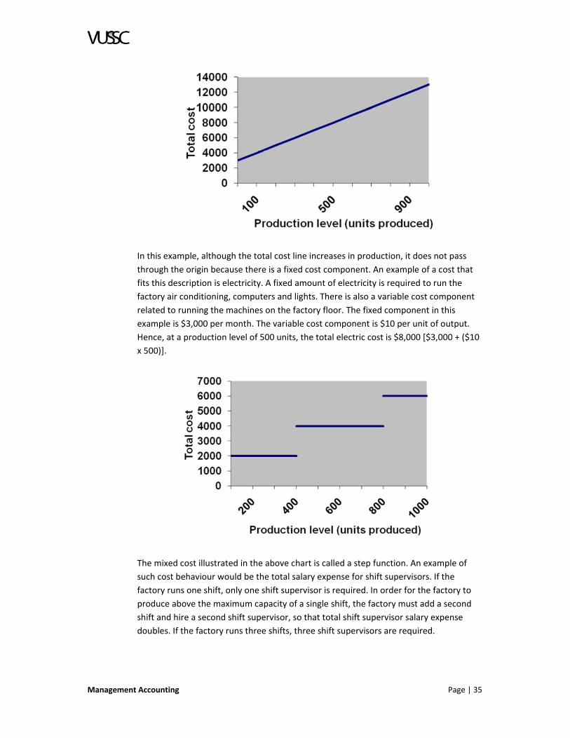
Management Accounting Page | 35
In this example, although the total cost line increases in production, it does not pass
through the origin because there is a fixed cost component. An example of a cost that
fits this description is electricity. A fixed amount of electricity is required to run the
factory air conditioning, computers and lights. There is also a variable cost component
related to running the machines on the factory floor. The fixed component in this
example is $3,000 per month. The variable cost component is $10 per unit of output.
Hence, at a production level of 500 units, the total electric cost is $8,000 [$3,000 + ($10
x 500)].
The mixed cost illustrated in the above chart is called a step function. An example of
such cost behaviour would be the total salary expense for shift supervisors. If the
factory runs one shift, only one shift supervisor is required. In order for the factory to
produce above the maximum capacity of a single shift, the factory must add a second
shift and hire a second shift supervisor, so that total shift supervisor salary expense
doubles. If the factory runs three shifts, three shift supervisors are required.

Page | 36 Management Accounting
COST BEHAVIOUR ASSUMPTIONS IN MANAGEMENT ACCOUNTING VERSUS
MICROECONOMICS
Microeconomic analysis usually assumes decreasing marginal costs of production,
sometimes followed by increasing marginal costs of production beyond a certain
production level. Hence, economists’ graphs of the total cost of production and the
average per‐unit cost of production show smooth, curved functions. Management
accountants usually assume the linear relationships depicted in the previous graphs.
Linearity is a more accurate description of many situations encountered by
management accountants than the economists’ curves, and even when linearity
constitutes a simplifying assumption it is almost always sufficiently descriptive for the
task at hand.
LESSON PROBLEMS
Now review the following problems and answer the related questions. Record your
answers in your course workbook.
Problem 1
A leading management accounting textbook (Cost Accounting: A Managerial Emphasis,
by Horngren, Datar and Foster, 12th edition) provides the following table (Exhibit 2‐5 in
that textbook) providing examples of cost classifications:
Direct Costs Indirect Costs
Variable
Costs:
Cost object: BMW X5s
produced
Example: Tires used in
assembly of automobile
Cost object: BMW X5’s produced
Example: Power costs at
Spartanburg plant. Power usage is
metered only to the plant, where
multiple products are assembled.
Fixed
Costs:
Cost object: BMW X5s
produced
Example: Salary of
supervisor on BMW X5
assembly line
Cost object: BMW X5s produced
Example: Annual lease costs at
Spartanburg plant. Lease is for
whole plant, where multiple
products are produced.
a. Evaluate whether the cost object is identical in each of the four boxes.
Problem 2
a. If a company makes 100 units of product, the allocated fixed cost per unit is $5
and the variable cost per unit is $6. What will be the per‐unit total cost (fixed
plus variable cost) if the company makes 200 units?

Management Accounting Page | 37
At a production and sales level of 1,000 units, the company’s costs are as
follows:
Variable manufacturing costs per unit $20
Allocated fixed manufacturing cost per unit $10
Variable selling costs per unit $ 5
Allocated fixed selling costs per unit $ 3
b. How much would the company have to spend in total (total cash outlay for both
fixed and variable costs), if it makes 1,200 units and sells 200 units (so that
1,000 units are in ending inventory at the end of the period)?
Problem 3
Describe each of the following costs as either fixed, variable, or semi‐variable (i.e.,
mixed):
a. The cost is $500 per unit at a production level of 50 units, and $500 per unit at a
production level of 100 units.
b. The cost is $500 in total at a production level of 50 units, and $1,000 in total at
a production level of 100 units.
c. The cost is $500 in total at a production level of 5 units, and $100 per unit at a
production level of 10 units.
Problem 4
If a company makes 100 units of product, the fixed cost per unit is $5 and the variable
cost per unit is $6.
a. How much will the company have to spend in total to make 200 units?
Problem 5
Identify the following cost as either fixed, variable or mixed (semi‐variable). The
horizontal axis refers to the number of units produced. The vertical axis refers to the
cost per unit at that level of production.

Page | 38 Management Accounting
Problem 6
Identify the following cost as either fixed, variable or mixed (semi‐variable). The
horizontal axis refers to the number of units produced. The vertical axis refers to the
total cost incurred for all of the units produced.
Problem 7
Identify the following cost as either fixed, variable or mixed (semi‐variable). The
horizontal axis refers to the number of units produced. The vertical axis refers to the
total cost incurred for all of the units produced.
Problem 8
Turquoise Company manufactures widgets and other good stuff. When 12,000 widgets
are produced, the total cost per widget is $40, calculated as follows:
Materials (a variable cost) $10
Labour (another variable cost) 15
Variable overhead (yet another variable cost) 10
Fixed overhead (not a variable cost) 5
The company is considering buying its widgets, instead of making them (hence, the
company would become a widget wholesaler, but will still manufacture other good
stuff). The company can buy widgets from another company for $42 per widget. If the
company stops making widgets, total fixed costs will not change, although some of the
facilities currently being used to make widgets can be rented out, resulting in $50,000 in
rental income to the Turquoise Company.
a. What would be the incremental cost or benefit to the Turquoise Company from
becoming a widget wholesaler instead of a widget manufacturer?

Management Accounting Page | 39
Problem 9
A particular cost is $10,000 in total when 50 units are made.
a. Complete the following table, indicating what the cost would be if production is
increased to 200 units:
Cost per Unit Cost in total
If this cost is a
variable cost
If this cost is a fixed
cost
b. Complete the following table, indicating what the cost would be if production is
reduced to 20 units:
Cost per Unit Cost in total
If this cost is a variable
cost
If this cost is a fixed
cost
Problem 10
Describe in two or three (no more than four) complete, well‐written sentences the
difference between fixed costs and variable costs.
Problem 11
In general, and within the relevant range, as production increases:
a. Per unit fixed costs and per unit variable costs both stay the same.
b. Per unit variable costs go down, and per unit fixed costs stay the same.
c. Per unit fixed costs go down, and per unit variable costs stay the same.
d. Per unit fixed costs and total variable costs both stay the same.
Problem 12
A particular cost is a semi‐variable (or mixed) cost, within a relevant range of 100 to 200
units of production. This cost is $1,000 in total when 100 units are manufactured (i.e.,
$10 per unit, when 100 units are manufactured). If production is doubled to 200 units,
which of the following is the most likely amount incurred for this particular cost?
a. $ 990
b. $1,000
Page | 40 Management Accounting
c. $1,100
d. $2,000
Problem 13
If production doubles, what will happen to variable costs?
a. Total variable costs and the variable cost per unit will both double.
b. Total variable costs will stay the same, and the variable cost per unit will
decrease
c. Total variable costs will stay the same, and the variable cost per unit will
double.
d. Total variable costs will double, and the variable cost per unit will stay the
same.
Problem 14
At a production level of 200 units, total costs for the factory are $9,000, consisting of
$8,000 in variable costs and $1,000 in fixed costs.
a. Calculate total factory costs if production increases 25%.
Problem 15 (The Matching Principle and Cost Behaviour)
Assume that the Little Rock Company calculates income in the following manner: All
manufacturing costs (variable and fixed) are treated as a cost of inventory, and the
“matching principle” is honoured for these costs, such that the cost to make inventory
appears on the Income Statement as Cost of Goods Sold when the inventory is sold. All
non‐manufacturing costs are expensed (appear on the Income Statement) when
incurred (i.e., the matching principle is not honoured for these costs).
In 2003, the Little Rock Company incurred fixed manufacturing costs of $500,000 and
fixed non‐manufacturing costs of $300,000. The Company made 10,000 units and sold
5,000. Variable manufacturing cost was $150 per unit. Variable non‐manufacturing cost
was $30 for every unit sold (this was a sales commission). Revenue was $3,000,000.
a. Calculate income for 2003.
LESSON SUMMARY
In this lesson you explored how to further estimate and use costs to manage the
production requirements of your business. Fixed costs do not impact production
whereas variable costs can increase or decrease productivity. You must be able to
identify what types of costs are fixed and what types are variable and manage them
accordingly.
In the next lesson we will examine the impact of cost on profitability.

Management Accounting Page | 41
LESSON 2.3: COST‐VOLUME‐PROFIT
LESSON INTRODUCTION
Cost–volume–profit (CVP), in managerial economics is a form of cost accounting. It is a
simplified model, useful for elementary instruction and for short‐run decisions.
CVP analysis expands the use of information provided by breakeven analysis. A critical
part of CVP analysis is the point where total revenues equal total costs (both fixed and
variable costs). At this break‐even point, a company will experience no income or loss.
This break‐even point can be an initial examination that precedes more detailed CVP
analysis.
We will examine the impact of CVP and how to complete a CVP analysis.
LESSON OBJECTIVES
Upon completion of this lesson you will be able to:
1. Explain the basic profit equation.
2. Describe the assumptions used in the CVP analysis.
3. Establish goals for profits using the targeted costing methods.
4. Complete an constrained analysis.
THE BASIC PROFIT EQUATION
Cost‐Volume‐Profit analysis (CVP) relates the firm’s cost structure to sales volume and
profitability. CVP analysis employs the same basic assumptions as in breakeven
analysis. The assumptions underlying CVP analysis are:
The behavior of both costs and revenues is linear throughout the relevant range
of activity. (This assumption precludes the concept of volume discounts on
either purchased materials or sales.)
Costs can be classified accurately as either fixed or variable.
Changes in activity are the only factors that affect costs.
All units produced are sold (there is no ending finished goods inventory).
When a company sells more than one type of product, the sales mix (the ratio
of each product to total sales) will remain constant.
The components of CVP analysis are:
Level or volume of activity
Unit selling prices
Variable cost per unit
Total fixed costs
Sales mix

Page | 42 Management Accounting
A formula that facilitates CVP analysis can be easily derived as follows:
This formula is henceforth called the Basic Profit Equation and is abbreviated:
CONTRIBUTION MARGIN
Contribution margin is defined as:
The unit contribution margin is defined as:
Typically, the Basic Profit Equation is used to solve one equation in one unknown,
where the unknown can be any of the elements of the equation. For example, given an
understanding of the firm’s cost structure and an estimate of sales volume for the
coming period, the equation predicts profits for the period. As another example, given
the firm’s cost structure, the equation indicates the required sales volume Q to achieve
a targeted level of profits P. If targeted profits are zero, the equation simplifies to:

Management Accounting Page | 43
In this case, Q indicates the required sales volume to break even, and the exercise is
called breakeven analysis.
CPV analysis can be depicted graphically. The graph below shows total revenue (SP x Q)
as a function of sales volume (Q), when the unit sales price (SP) is $12.
The following graph shows the total cost function when fixed costs (FC) are $4,000 and
the variable cost per unit (VC) is $5.
The following graph combines the revenue and cost functions depicted in the previous
two graphs into a single graph.

Page | 44 Management Accounting
The intersection of the revenue line and the total cost line indicates the breakeven
volume, which in this example, occurs between 571 and 572 units. To the left of this
point, the company incurs a loss. To the right of this point, the company generates
profits. The amount of profit or loss can be measured as the vertical distance between
the revenue line and the total cost line.
ASSUMPTIONS IN CVP ANALYSIS
The Basic Profit Equation relies on a number of simplifying assumptions.
Only one product is sold. However, multiple products can be accommodated by using
an average sales mix and restating Q, SP and VC in terms of a representative bundle of
products. For example, a hot dog vendor might calculate that the “average” customer
buys two hot dogs, one bag of chips, and two‐thirds of a beverage. Q is the number of
customers, and SP and VC refer to the sales price and variable cost for this “average”
customer order.
If the equation is applied to a manufacturer, beginning inventory is assumed equal to
zero, and production is assumed equal to sales. Relaxing these assumptions requires
additional structure on the equation, including specifying an inventory flow assumption
(e.g., FIFO or LIFO) and the extent to which the matching principle is honoured for
manufacturing costs.
The analysis is confined to the relevant range. In other words, fixed costs remain
unchanged in total, and variable costs remain unchanged per unit, over the range of Q
under consideration.
TARGET COSTING
A relatively recent innovation in product planning and design is called target costing. In
the context of the Basic Profit Equation, target costing sets a goal for profits, and solves
for the unit variable cost required to achieve those profits. The design and
manufacturing engineers are then assigned the task of building the product for a unit
cost not to exceed the target. This approach differs from a more traditional product
design approach, in which design engineers (possibly with input from merchandisers)

Management Accounting Page | 45
design innovative products, manufacturing engineers then determine how to make the
products, cost accountants then determine the manufacturing costs, and finally,
merchandisers and sales personnel set sales prices. Hence, setting the sales price comes
last in the traditional approach, but it comes first in target costing.
Target costing is appropriate when SP and Q are predictable, but are not choice
variables, such as might occur in well‐established competitive markets. In such a setting,
merchandisers might know the price that they want to charge for the product, and can
probably estimate the sales volume that will be achieved at that price. Target costing
has been used successfully by a number of companies including Toyota, which
redesigned the Camry around the turn of the century as part of a target costing
strategy.
CONSTRAINED RESOURCES
Contribution margin analysis plays an important role when a multi‐product organization
has a binding resource constraint. The resource constraint can take many forms, such as
production throughput on a critical machine, freezer space, or skilled labour hours in a
particular function. In the presence of a resource constraint, the optimal production
decision is to maximize the contribution margin per unit of the constraint.
For example, assume that a company makes small widgets and large widgets. Small
widgets incur $5 in variable manufacturing and non‐manufacturing costs, and sell for
$10. Large widgets incur $11 in variable manufacturing and non‐manufacturing costs,
and sell for $15. If production throughput is constrained by the capacity of a particular
machine, and both small and large widgets require one hour of processing time on that
machine, then the company should make only small widgets, because small widgets
provide a contribution margin of $5 per unit, whereas large widgets provide a
contribution margin of $4 per unit. On the other hand, if each small widget requires two
hours of processing time on the machine, and large widgets require only one hour, then
the company should make only large widgets, calculated as follows:
Small widgets: contribution margin per machine hour = ($10 $5) ÷ 2 = $2.50 per hour
Large widgets: contribution margin per machine hour = ($15 $11) ÷ 1 = $4.00 per hour
The company maximizes profits by making large widgets, even though large widgets
have a lower contribution margin per unit than small widgets, because large widgets
require less machine time and hence, are more efficient with respect to the limited
resource. In other words, the large widgets generate a higher contribution margin per
hour on the machine that constitutes the capacity constraint of the factory.
LEVERAGE
There is often a trade‐off between fixed cost inputs and variable cost inputs. For
example, in the manufacturing sector, a company can build its own factory (thereby
operating with relatively high fixed costs but relatively low variable costs) or outsource
production (operating with relatively low fixed costs but relatively high variable costs). A
merchandising company can pay its sales force a flat salary (relatively higher fixed costs)
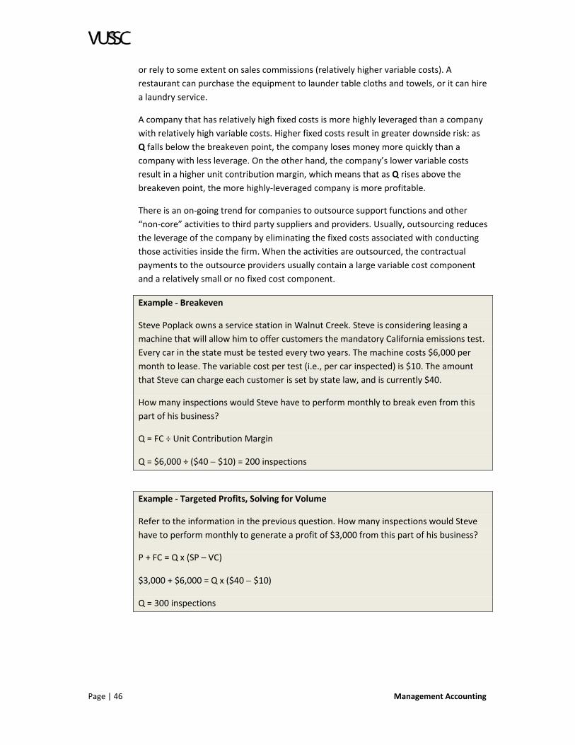
Page | 46 Management Accounting
or rely to some extent on sales commissions (relatively higher variable costs). A
restaurant can purchase the equipment to launder table cloths and towels, or it can hire
a laundry service.
A company that has relatively high fixed costs is more highly leveraged than a company
with relatively high variable costs. Higher fixed costs result in greater downside risk: as
Q falls below the breakeven point, the company loses money more quickly than a
company with less leverage. On the other hand, the company’s lower variable costs
result in a higher unit contribution margin, which means that as Q rises above the
breakeven point, the more highly‐leveraged company is more profitable.
There is an on‐going trend for companies to outsource support functions and other
“non‐core” activities to third party suppliers and providers. Usually, outsourcing reduces
the leverage of the company by eliminating the fixed costs associated with conducting
those activities inside the firm. When the activities are outsourced, the contractual
payments to the outsource providers usually contain a large variable cost component
and a relatively small or no fixed cost component.
Example ‐ Breakeven
Steve Poplack owns a service station in Walnut Creek. Steve is considering leasing a
machine that will allow him to offer customers the mandatory California emissions test.
Every car in the state must be tested every two years. The machine costs $6,000 per
month to lease. The variable cost per test (i.e., per car inspected) is $10. The amount
that Steve can charge each customer is set by state law, and is currently $40.
How many inspections would Steve have to perform monthly to break even from this
part of his business?
Q = FC ÷ Unit Contribution Margin
Q = $6,000 ÷ ($40 $10) = 200 inspections
Example ‐ Targeted Profits, Solving for Volume
Refer to the information in the previous question. How many inspections would Steve
have to perform monthly to generate a profit of $3,000 from this part of his business?
P + FC = Q x (SP – VC)
$3,000 + $6,000 = Q x ($40 $10)
Q = 300 inspections

Management Accounting Page | 47
Example ‐ Targeted Profits, Solving for Sales Price
Alice Waters (age 9) runs a lemonade stand in the summer in Palo Alto, California. Her
daily fixed costs are $20. Her variable costs are $2 per glass of ice‐cold, refreshing,
lemonade. Alice sells an average of 100 glasses per day. What price would Alice have to
charge per glass, in order to generate profits of $200 per day?
P + FC = Q x (SP – VC)
$200 + $20 = 100 x (SP $2)
SP = $4.20 per glass
Example ‐ Contribution Margin
Refer to the previous question. What price would Alice have to charge per glass, in
order to generate a total contribution margin of $200 per day?
Total CM = Q x (SP – VC)
$200 = 100 x (SP $2.00)
SP = $4.00 per glass
Example ‐ Target Costing
Refer to the information about Alice, but now assume that Alice wants to charge $3 per
glass of lemonade, and at this price, Alice can sell 110 glasses of lemonade daily.
Applying target costing, what would the variable cost per glass have to be, in order to
generate profits of $200 per day?
P + FC = Q x (SP – VC)
$200 + $20 = 110 x ($3 – VC)
VC = $1
LESSON PROBLEMS
Now review the following problems and answer the related questions. Record your
answers in your course workbook.
Problem 1
Sara, Sarah, Shara and Associates want to earn a total contribution margin of $10,000
on sales of 1,000 units. Their sales price is $15 per unit, and their fixed costs are $5,000.
a. What variable cost per unit is necessary to achieve their goal?

Page | 48 Management Accounting
Problem 2
George and Gracie both make the same product, and sell it for the same sales price.
Gracie has a higher variable cost per unit than George. George has higher fixed costs
than Gracie. Who has the higher breakeven point, in terms of number of units sold?
a. Gracie has a higher breakeven point than George.
b. George has a higher breakeven point than Gracie.
c. Gracie and George have the same breakeven point.
d. Impossible to ascertain, from the information given.
Problem 3
The Virginia Company has fixed costs of $100,000 per month, and variable costs of $30
per unit of output. The sales price is $50 per unit of output.
a. How many units would the company have to sell per month, to generate profits
of $30,000 per month?
Problem 4
The Charleston Company has fixed costs of $20,000 per month, and variable costs of
$15 per unit of output. The company would like to earn profits of $4,000 per month.
a. At a sales volume of 12,000 units per month, what sales price per unit would
the company have to charge in order to achieve its targeted monthly profit?
Problem 5
The Delaware Company has fixed costs of $100,000 per year and variable costs of $10
per unit of output. The Pennsylvania Company has fixed costs of $120,000 per year and
variable costs of $9 per unit of output. The sales price per unit is the same for both
companies.
a. Identify a sales price at which both companies will have the same break‐even
point in terms of number of units sold.
Problem 6
The Biloxi Company has the following cost structure: fixed costs of $70,000 per month
and variable costs of $50 per unit. The Birmingham Company has the following cost
structure: fixed costs of $60,000 per month and variable costs of $60 per unit. Both
companies make the same product, which sells for $100 per unit. There is a sales level
at which these two companies earn the same profits.
a. What is that sales level?
b. Which company is more profitable as sales volume exceeds this sales level?

Management Accounting Page | 49
Problem 7
Company X and Company Y sell the same product for the same price. Company X has
fixed costs of $100 and variable costs of $10 per unit. Company Y has fixed costs of $200
and variable costs of $8.
a. What is the unit sales price at which these companies will have the same break‐
even point in terms of unit sales?
Problem 8
Eliza sells flowers in Covent Garden. Her fixed costs are $50 per day. Her average sales
price is $4 per flower. She is currently selling 400 flowers per day. Her current variable
cost is $3 per flower. Eliza anticipates that her daily sales will increase to 500 flowers
per day.
a. How much could her variable cost per flower increase for her to still earn the
same daily profits as before?
Problem 9: The following information is available for the publisher of “Frank the Cow
Dog” Children’s Books:
Variable cost: $10.00 per book
Sales price: $15.00 per book
Fixed costs: $35,000 per year
These costs apply over a relevant range of the production of one book to the production
of 40,000 books.
a. What is the contribution margin per unit?
b. What would operating income be at a sales level of 15,000 books?
c. What is the breakeven point in units?
d. Ignore the sales price of $15 per book. What would the sales price have to be
for the publisher to earn operating income of $165,000 on sales of 25,000
books?
Problem 10
The Emerald Street Ice Cream Shop sells ice cream cones. The store’s cost structure is as
follows: fixed costs per month are $2,000. Variable costs are $1.50 for a single scoop
cone and $1.75 for a double scoop cone.
a. If Emerald Street only sells double scoop cones, and sells them for $4.25 per
cone, what is the break‐even point in units?
b. If Emerald Street only sells single scoop cones, and charges $3.50 per cone, how
many ice cream cones would Emerald Street have to sell to make a profit of
$3,000 per month?

Page | 50 Management Accounting
c. Assume that Emerald Street wants to sell only double scoop cones, and believes
it can sell 8,000 cones per month at $4.25 per cone. What would the variable
cost per cone have to be for Emerald Street to make a profit of $8,000 per
month?
d. Ignore Part (C) and refer to the original information. If Emerald Street only sells
single scoop cones, and sells 5,000 cones per month for $3.60 per cone, what is
the contribution margin per unit?
Problem 11
Teddy Bear Fudge Company makes two types of fudge: plain fudge and fudge with nuts.
Following is information about the company’s cost structure when 1,000 pounds of
fudge are produced. There is no direct labour.
Overhead Plain Fudge Fudge with
Nuts
Per unit information:
Sales price per pound
Direct materials per pound
Sales commission per pound
Variable overhead
Fixed costs:
Fixed manufacturing
overhead
Fixed non‐manufacturing
overhead
$500
$2,000
$300
$8.00
$2.00
$0.50
$8.00
$2.25
$0.50
a. Assuming that variable overhead costs are linear in the quantity of production
(i.e., pounds of fudge), and assuming that 50% of sales are plain fudge, and 50%
of sales are fudge with nuts, calculate the breakeven point in pounds of fudge
LESSON SUMMARY
Understanding how to estimate the cost to produce your product and establish a sales
price is an important skill for all entrepreneurs. You must determine what your
breakeven point is and when the business will become profitable. Ideally this happens
sooner than later and is reflected in your financial plan.
In your first course in accounting you learned how to create a budget. In the next
lesson you will explore the concept of flexible budgeting and its impact on a business.

Management Accounting Page | 51
LESSON 2.4: FLEXIBLE BUDGETING
LESSON INTRODUCTION
A budget is a plan for the future. Hence, budgets are planning tools, and they are
usually prepared prior to the start of the period being budgeted. However, the
comparison of the budget to actual results provides valuable information about
performance. Therefore, budgets are both planning tools and performance evaluation
tools. In this lesson we will explore the approach to flexible budgeting.
LESSON OBJECTIVES
Upon completion of this lesson you will be able to:
1. Describe the difference between a static and flexible budget.
2. Calculate budget variance.
3. Produce a flexible budget.
BUDGETS
Usually, the single most important input in the budget is some measure of anticipated
output. For a factory, this measure of output is the number of units of each product
produced. For a retailer, it might be the number of units of each product sold. For a
hospital, it is the number of patient days (the number of patient admissions multiplied
by the average length of stay).
The static budget is the budget that is based on this projected level of output, prior to
the start of the period. In other words, the static budget is the “original” budget. The
static budget variance is the difference between any line‐item in this original budget
and the corresponding line‐item from the statement of actual results. Often, the line‐
item of most interest is the “bottom line”: total cost of production for the factory and
other cost centres; income for profit centres.
The flexible budget is a performance evaluation tool. It cannot be prepared before the
end of the period. A flexible budget adjusts the static budget for the actual level of
output. The flexible budget asks the question: “If I had known at the beginning of the
period what my output volume (units produced or units sold) would be, what would my
budget have looked like?” The motivation for the flexible budget is to compare apples to
apples. If the factory actually produced 10,000 units, then management should
compare actual factory costs for 10,000 units to what the factory should have spent to
make 10,000 units, not to what the factory should have spent to make 9,000 units or
11,000 units or any other production level.
The flexible budget variance is the difference between any line‐item in the flexible
budget and the corresponding line‐item from the statement of actual results.

Page | 52 Management Accounting
PREPARING A FLEXIBLE BUDGET
The following steps are used to prepare a flexible budget:
1. Determine the budgeted variable cost per unit of output. Also determine the
budgeted sales price per unit of output, if the entity to which the budget applies
generates revenue (e.g., the retailer or the hospital).
2. Determine the budgeted level of fixed costs.
3. Determine the actual volume of output achieved (e.g., units produced for a
factory, units sold for a retailer, patient days for a hospital).
4. Build the flexible budget based on the budgeted cost information from steps 1
and 2, and the actual volume of output from step 3.
Flexible budgets are prepared at the end of the period, when actual output is known.
However, the same steps described above for creating the flexible budget can be used
prior to the start of the period to anticipate costs and revenues for any projected level
of output, where the projected level of output is incorporated at step 3. If these steps
are applied to various anticipated levels of output, the analysis is called pro forma
analysis. Pro forma analysis is useful for planning purposes. For example, if next year’s
sales are double this year’s sales, what will be the company’s cash, materials, and
labour requirements in order to meet production needs?
PRO FORMA ANALYSIS AT GUESS WHO JEANS
Following are pro forma monthly income statements for Guess Who Jeans, a small,
start‐up fashion jeans manufacturer. The pro forma analysis was prepared at the
beginning of the month and considered three alternative sales levels. The company has
no variable marketing costs.
GUESS WHO JEANS PRO FORMA ANALYSIS
FOR THE UPCOMING MONTH
Income Statement line‐item
Budgeted amount per unit
Pro Forma Analysis for Alternative Output Levels
10,000 units 20,000 units 30,000 units
Revenue
Variable costs:
Materials
Labour
Overhead
Total
Contribution margin
$40
15
10
5
30
$10
$400,000
150,000
100,000
50,000
300,000
100,000
$800,000
300,000
200,000
100,000
600,000
200,000
$1,200,000
450,000
300,000
150,000
900,000
300,000
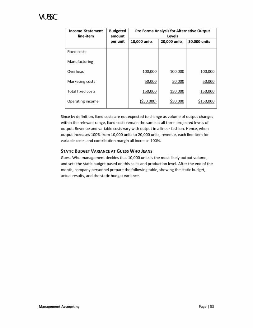
Management Accounting Page | 53
Income Statement line‐item
Budgeted amount per unit
Pro Forma Analysis for Alternative Output Levels
10,000 units 20,000 units 30,000 units
Fixed costs:
Manufacturing
Overhead
Marketing costs
Total fixed costs
Operating income
100,000
50,000
150,000
($50,000)
100,000
50,000
150,000
$50,000
100,000
50,000
150,000
$150,000
Since by definition, fixed costs are not expected to change as volume of output changes
within the relevant range, fixed costs remain the same at all three projected levels of
output. Revenue and variable costs vary with output in a linear fashion. Hence, when
output increases 100% from 10,000 units to 20,000 units, revenue, each line‐item for
variable costs, and contribution margin all increase 100%.
STATIC BUDGET VARIANCE AT GUESS WHO JEANS
Guess Who management decides that 10,000 units is the most likely output volume,
and sets the static budget based on this sales and production level. After the end of the
month, company personnel prepare the following table, showing the static budget,
actual results, and the static budget variance.

Page | 54 Management Accounting
GUESS WHO JEANS STATIC BUDGET VARIANCE
FOR THE MONTH JUST ENDED
Income Statement line‐item
Budgeted amount per unit
StaticBudget (A)
10,000 units
ActualResults (B)
16,000 units
StaticBudget Variance (A) – (B)
Revenue
Variable costs:
Materials
Labour
Overhead
Total
Contribution margin
Fixed costs:
Manufacturing
Overhead
Marketing costs
Total fixed costs
Operating income
$40
15
10
5
30
$10
$400,000
150,000
100,000
50,000
300,000
100,000
100,000
50,000
150,000
($50,000)
$670,000
230,000
167,000
84,000
481,000
189,000
105,000
49,000
154,000
$35,000
$270,000
(80,000)
(67,000)
(34,000)
(181,000)
89,000
(5,000)
1,000.
(4,000)
$85,000
In the variance column, positive numbers are favourable variances (good news), and
negative numbers are unfavourable (bad news).
The static budget variance shows a large favourable variance for revenue, and large
unfavourable variances for variable costs. These large variances are due primarily to the
fact that the static budget was built on an output level of 10,000 units, while the
company actually made and sold 16,000 units. The revenue variance might also be due
to an average unit sales price that differed from budget. The variable cost variances
might also be due to input prices that differed from budget (e.g., the price of fabric), or
input quantities that differed from the per‐unit budgeted amounts (e.g., yards of fabric
per pair of pants).
There are also small variances for fixed costs. These costs should not vary with the level
of output (at least within the relevant range). However, many factors can cause actual
fixed costs to differ from budgeted fixed costs that are unrelated to output volume. For
example, property tax rates and the fixed salaries of front office personnel can change,

Management Accounting Page | 55
and depreciation expense can change if unexpected capital acquisitions or dispositions
occur.
THE FLEXIBLE BUDGET VARIANCE AT GUESS WHO JEANS
In order to better understand the causes of the large revenue and variable cost
variances in the static budget variance column, Guess Who personnel prepare the
following flexible budget.
GUESS WHO JEANS FLEXIBLE BUDGET VARIANCE FOR THE MONTH JUST ENDED
Income Statement line‐item
Budgeted amount per unit
Flexible Budget (A)
16,000 units
ActualResults (B)
16,000 units
Flexible Budget Variance (A) – (B)
Revenue
Variable costs:
Materials
Labour
Overhead
Total
Contribution margin
Fixed costs:
Manufacturing
Overhead
Marketing costs
Total fixed costs
Operating income
$40
15
10
5
30
$10
$640,000
240,000
160,000
80,000
480,000
160,000
100,000
50,000
150,000
$10,000
$670,000
230,000
167,000
84,000
481,000
189,000
105,000
49,000
154,000
$35,000
$30,000
10,000.
(7,000)
(4,000)
(1,000)
29,000
(5,000)
1,000.
(4,000)
$25,000
Once again, positive variances are favourable (good news), and negative variances are
unfavourable (bad news).
From this table, Guess Who management sees that even after adjusting for sales
volume, revenue was higher than would have been expected. The favourable $30,000
variance must be due entirely to an average sales price that was higher than planned
(almost $42 per pair compared to the original budget of $40 per pair).

Page | 56 Management Accounting
Materials costs were lower than would have been expected for a sales volume of 16,000
units. This favourable variance could be due to lower fabric prices, or to more efficient
utilization of fabric (less waste than expected), or a combination of these two factors.
Labour and overhead were higher than expected, even after adjusting for the sales
volume of 16,000 units. This unfavourable flexible budget variance implies that either
wage rates were higher than planned, or labour was not as efficient as planned, or both.
Similarly, the components of variable overhead were either more expensive than
budgeted, or were used more intensively than budgeted. For example, electric rates
might have been higher than planned, or more electricity was used than planned per
unit of output.
The fixed cost variances are identical in this table to the previous table. In other words,
the flexible budget and flexible budget variance provide no additional information
about fixed costs beyond what can be learned from the static budget variance.
LESSON PROBLEMS
Now review the following problems and answer the related questions. Record your
answers in your course workbook.
Problem 1
The Silver Company planned to make 10,000 units of product in July. Budgeted costs
were $110,000 in variable costs and $220,000 in fixed costs. The company actually
made 11,000 units. Actual costs incurred were $110,000 in variable costs and $210,000
in fixed costs. Calculate the flexible budget variance for July.
a. Is it favourable or unfavourable?
Problem 2
The Davenport Problem H Club plans to spend $5,000 to send 20 of its members to the
State Fair in Des Moines. $2,000 of the $5,000 are fixed costs. Twenty‐five members
actually attend the fair, at a cost of $6,000.
a. Calculate the flexible budget variance.
b. Is it favourable or unfavourable?
Problem 3
A piano teacher has budgeted fixed costs of $1,250 per month, and budgeted variable
costs of $1,200 per month, where variable costs are a linear function of the number of
one‐hour piano lessons. The piano teacher expected to give 120 one‐hour piano lessons
in April, but actually gave 150 one‐hour piano lessons in April. Actual fixed costs were
$1,000 and actual variable costs were $1,500.
a. What is the flexible budget variance for April?
b. Is it favourable or unfavourable?

Management Accounting Page | 57
Problem 4
The Amber Company planned to make 1,000 units of product in June. The static budget
showed a per‐unit cost of $10, which consisted of $3 for variable costs and $7 for
allocated fixed overhead. The company actually made 1,100 units. The actual per‐unit
cost was $10, which consisted of $3 for variable costs and $7 for allocated fixed
overhead.
a. Calculate the total flexible budget variance for June.
b. Is it favourable or unfavourable?
Problem 5
The static budget (i.e., the original budget) of the Tam‐Taha Corporation showed a
production cost of $10 per unit at a production level of 100 units. This $10 included $2
of fixed costs. Actual production was 200 units, and actual costs were $9 per unit, which
included $1 of fixed costs.
a. Calculate the flexible budget variance.
b. Is it favourable or unfavourable?
Problem 6
MDC company plans to make 7,000 units, and at this level of production, the cost per
unit would be $50. This $50 consists of $30 in variable costs and $20 in allocated fixed
overhead.
a. What would the flexible budget show for total costs, if the company makes
6,000 units?
Problem 7
Kinney‐Borst anticipates production and sales of 100 units, total variable costs of
$6,000, and total fixed costs of $3,000. Actual production and sales were 200 units.
a. Calculate a flexible budget.
Problem 8
At the beginning of the year, a company budgets variable costs of $2,000 and fixed costs
of $1,500 at a production level of 100 units. The company actually produces 110 units,
and incurs variable costs of $2,000 and fixed costs of $1,800.
a. What is the flexible budget variance?
b. Is it favourable or unfavourable?

Page | 58 Management Accounting
Problem 9
CWC Company planned to make 2,100 units in 2005, and budgeted $900,000 in fixed
costs and $130 per unit for variable costs. CWC actually made 2,000 units in 2005, and
incurred total costs of $1,200,000.
a. What is the flexible budget variance for 2005?
b. Is it favourable or unfavourable?
Problem 10
Iron Butterfly, Inc., manufactures a single model of a deluxe portable camping stove.
Information for August production is as follows:
Budgeted Actual
Variable Costs, per unit $50 $52
Fixed Costs for August
Production for August
$2,500,000
40,000 units
$2,150,000
38,000 units
a. What is the flexible budget variance for August?
Problem 11
The Pretenders, Inc., produces exercise equipment for dogs. The following information
pertains to variable manufacturing overhead, which is allocated using machine hours.
Budget Actual
Units produced
Machine hours
Variable manufacturing overhead
15,000
5,000
$161,250
22,000
7,500
$242,000
a. Calculate the flexible budget variance.
Problem 12
The Bee Gees cultivate and sell honey. They provide you the following data with respect
to the upcoming year.
Budgeted variable costs (per jar):
Cost of the jar & label $1.50
Labour 2.40
First aid supplies .25
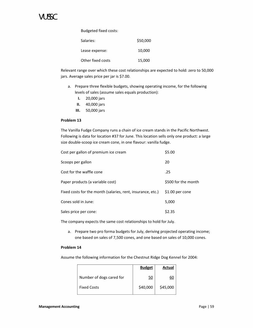
Management Accounting Page | 59
Budgeted fixed costs:
Salaries: $50,000
Lease expense: 10,000
Other fixed costs 15,000
Relevant range over which these cost relationships are expected to hold: zero to 50,000
jars. Average sales price per jar is $7.00.
a. Prepare three flexible budgets, showing operating income, for the following
levels of sales (assume sales equals production):
I. 20,000 jars
II. 40,000 jars
III. 50,000 jars
Problem 13
The Vanilla Fudge Company runs a chain of ice cream stands in the Pacific Northwest.
Following is data for location #37 for June. This location sells only one product: a large
size double‐scoop ice cream cone, in one flavour: vanilla fudge.
Cost per gallon of premium ice cream $5.00
Scoops per gallon 20
Cost for the waffle cone .25
Paper products (a variable cost) $500 for the month
Fixed costs for the month (salaries, rent, insurance, etc.) $1.00 per cone
Cones sold in June: 5,000
Sales price per cone: $2.35
The company expects the same cost relationships to hold for July.
a. Prepare two pro forma budgets for July, deriving projected operating income;
one based on sales of 7,500 cones, and one based on sales of 10,000 cones.
Problem 14
Assume the following information for the Chestnut Ridge Dog Kennel for 2004:
Number of dogs cared for
Fixed Costs
Budget
50
$40,000
Actual
60
$45,000
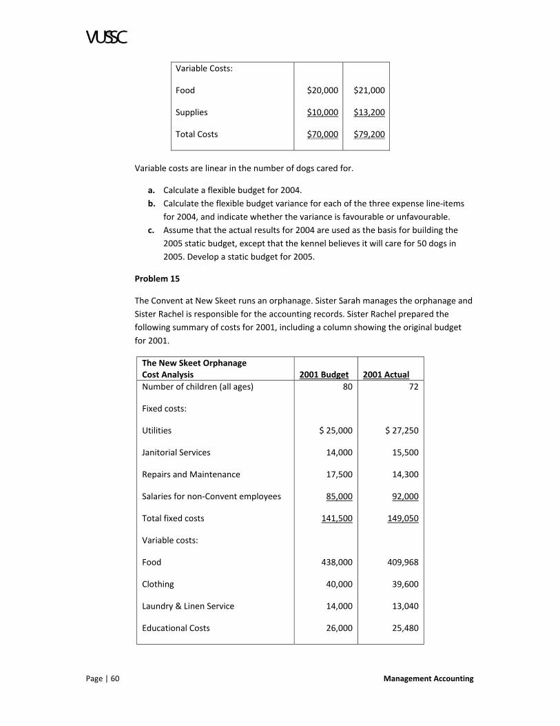
Page | 60 Management Accounting
Variable Costs:
Food
Supplies
Total Costs
$20,000
$10,000
$70,000
$21,000
$13,200
$79,200
Variable costs are linear in the number of dogs cared for.
a. Calculate a flexible budget for 2004.
b. Calculate the flexible budget variance for each of the three expense line‐items
for 2004, and indicate whether the variance is favourable or unfavourable.
c. Assume that the actual results for 2004 are used as the basis for building the
2005 static budget, except that the kennel believes it will care for 50 dogs in
2005. Develop a static budget for 2005.
Problem 15
The Convent at New Skeet runs an orphanage. Sister Sarah manages the orphanage and
Sister Rachel is responsible for the accounting records. Sister Rachel prepared the
following summary of costs for 2001, including a column showing the original budget
for 2001.
The New Skeet OrphanageCost Analysis 2001 Budget 2001 Actual
Number of children (all ages)
Fixed costs:
Utilities
Janitorial Services
Repairs and Maintenance
Salaries for non‐Convent employees
Total fixed costs
Variable costs:
Food
Clothing
Laundry & Linen Service
Educational Costs
80
$ 25,000
14,000
17,500
85,000
141,500
438,000
40,000
14,000
26,000
72
$ 27,250
15,500
14,300
92,000
149,050
409,968
39,600
13,040
25,480

Management Accounting Page | 61
The New Skeet OrphanageCost Analysis 2001 Budget 2001 Actual
Allowances
Total variable costs
Total costs
20,000
538,000
$679,500
25,000
513,088
$662,138
Sister Sarah is very concerned that the orphanage uses its funds efficiently. She is
pleased that total costs were below budget for the year, but she wonders if this is partly
due to the fact that the orphanage housed fewer children than expected for the year.
a. Prepare a flexible budget for 2001, based (i.e., “flexed”) on the number of
children actually housed in 2001.
b. Should Sister Sarah be satisfied with the orphanage’s cost management in
2001? Briefly explain.
LESSON SUMMARY
In this lesson we explored the use of flexible budgeting and its impact on profit and loss.
We learned that positive numbers are favourable variances (good news), and negative
numbers are unfavourable (bad news). In the next lesson we will explore some
additional concepts related to cost variance.

Page | 62 Management Accounting
LESSON 2.5: COST VARIANCES FOR DIRECT MATERIALS AND LABOUR
LESSON INTRODUCTION
In the previous Lesson, we saw that the static budget variance measures the difference
between budgeted costs and actual costs (or budgeted revenues and actual revenues).
We also saw that when the actual volume of output (sales or production) differs from
the budgeted volume of output, this difference contributes to the static budget
variance. We saw that a flexible budget adjusts the static budget to reflect what the
budget would have looked like, if the actual output volume could have been known in
advance. The flexible budget variance measures the difference between the flexible
budget and actual results. In this lesson we will explore additional types of variance
for materials and labour costs.
LESSON OBJECTIVES
Upon completion of this lesson you will be able to:
1. Define Notation.
2. Explain derivation of the direct materials variances.
3. Calculate geometric representation of the direct materials variances.
4. Discuss the timing of recognition of the price variance.
5. Calculate cost variances and external reporting.
6. Calculate cost variances for direct labour.
DIFFERENT VARIANCE FOR VARIABLE COSTS
As stated in the previous lesson, there can be only two explanations for the flexible
budget variance for variable costs. First, there can be a difference between budgeted
input prices and actual input prices: the company paid more per yard of fabric, or less
per pound of steel, than planned. Second, there can be an efficiency piece: the
company used more fabric per pair of pants, or fewer pounds of steel per widget, than
planned. In this Lesson, we separate the flexible budget variance for direct materials
into these two pieces: the “price” piece, and the “efficiency” piece. At the end of the
Lesson, we extend the discussion to other variable costs: direct labour and variable
overhead.
Notation:
The following concepts and abbreviations are used:
Inputs are the materials used in the production process (fabric or steel).
Outputs are the units of finished product (pairs of pants, or widgets).
Abbreviation Definition Explanation
Q
Quantity
The total quantity of inputs used in production.
(the inputs for all output units, not the inputs
for one unit of output)

Management Accounting Page | 63
Abbreviation Definition Explanation
P
AP
SP
AQ
SQ
Price
Actual Price
Standard Price
Actual Quantity
Standard
Quantity
The price per unit of input
The actual price paid per unit of input
The budgeted price paid per unit of input
The actual quantity of inputs used in production
The quantity of inputs that “should have been
used” for the actual output produced
Sometimes Q refers to the total quantity of inputs purchased, not used in production.
We will return to this possibility later in this Lesson, but for now, Q refers to the
quantity used in production.
The most important concept identified above is the Standard Quantity (SQ). SQ is a
flexible budget concept: it is the quantity of inputs that would have been budgeted had
the budget correctly anticipated the actual volume of output.
DERIVATION OF THE DIRECT MATERIALS VARIANCES:
Given these definitions, the flexible budget can be expressed as:
and the flexible budget variance can be expressed as:
We introduce the following expression:
This expression measures what the company “should have spent” for the actual
quantity of inputs used. We can insert this expression into Equation (1) in order to
separate the flexible budget variance into two pieces:
Q P AP
SP
AQ
SQ
QuantityPrice Actual Price Standard Price Actual Quantity Standard Quantity

Page | 64 Management Accounting
The first term minus the second term in Equation (2) can be rewritten as follows:
This expression is the price variance. It is the actual inputs used in
production (AQ) multiplied by the difference between the budgeted
price (SP) and the actual price (AP) paid per unit of input. The price
variance is abbreviated PV. Hence:
If the term in parenthesis is positive, the factory paid more per unit
of input than budgeted, and the price variance is unfavourable. If the term in
parenthesis is negative, the factory paid less per unit of input than budgeted, and the
price variance is favourable. In either case, the price variance can be interpreted as
answering the following question: What was the total impact on the cost of production
caused by the fact that the actual price per unit of input differed from the budgeted
price.
The second term minus the third term in Equation (2) can be rewritten as follows:
This expression is the quantity variance (also called the usage variance). It is the
budgeted price per unit of input (SP) multiplied by the difference between the quantity
of inputs that should have been used for the output units produced (SQ) and the
quantity of inputs actually used (AQ). The quantity variance is abbreviated QV. Hence:
If the term in parenthesis is positive, the factory used more inputs than it should have
used for the amount of output units produced, and the quantity variance is
unfavourable. If the term in parenthesis is negative, the factory used fewer inputs than
it should have used for the amount of output units produced, and the quantity variance
is favourable. In either case, the quantity variance can be interpreted as answering the
following question: What was the total impact on the cost of production caused by the
fact that the quantity of inputs used to make each unit of output differed from budget.
Q P AP SP
AQ
SQ
QuantityPrice Actual Price Standard Price Actual Quantity Standard Quantity

Management Accounting Page | 65
GEOMETRIC REPRESENTATION OF THE DIRECT MATERIALS VARIANCES
The following table shows the price and quantity variances graphically, when both
variances are negative. The area of the yellow box represents the flexible budget. The
area of the “outer” box (the union of the three coloured boxes) represents the actual
amount incurred for direct materials. The price variance is the area of the orange box,
and the quantity variance is the area of the green box. It is easy to see from this
geometric representation that the difference between the flexible budget and actual
costs consists of two variances: the price variance and the quantity variance.
The following table is identical to the one shown above except for the upper right‐hand
corner. This table shows that the formula for the price variance includes an
“interactive” variance that only exists when both AP SP and AQ SQ. If AQ = SQ, this interactive variance box collapses from the right. If AP = SP, this box collapses from the
top.
There is no theoretical justification for treating this interactive variance as part of the
price variance instead of part of the quantity variance, but it is customarily assigned to
the price variance or else reported separately.

Page | 66 Management Accounting
TIMING OF RECOGNITION OF THE PRICE VARIANCE
Some firms recognize the price variance for direct materials when the raw materials are
purchased, rather than waiting until the raw materials are put into production. In this
case, the AQ in the price variance will generally differ from the AQ in the quantity
variance, which is denoted in the following expressions for these variances:
Recognizing the price variance when raw materials are purchased provides more timely
information to management about the cost of direct materials and the performance of
the purchasing department. Hence, this method for calculating the price variance has
much to commend it. However, in this situation, the sum of the price variance and
quantity variance will not equal the flexible budget variance, except by coincidence or
when beginning and ending quantities of raw materials are zero.
COST VARIANCES AND EXTERNAL REPORTING
Cost variances are not reported separately in the external financial statements of a firm,
but are implicitly incorporated in one or more line‐items on the balance sheet and
income statement, such as Cost of Goods Sold and ending Finished Goods Inventory.
However, for internal reporting, cost variances are frequently reported as separate line‐
items on divisional income statements and product‐specific profit statements.
COST VARIANCES FOR DIRECT LABOUR
The formulas for splitting the flexible budget variance into a
“price” variance and “quantity” variance are the same for direct
labour as direct materials. However, the terminology differs
slightly. What is called the price variance for direct materials is
called the rate variance or wage rate variance for direct labour.
However, we retain the same abbreviations:
where AQ is the actual labour hours used in production, AP is the
actual wage rate, and SP is the budgeted wage rate.
What is called the quantity or usage variance for direct materials is called the efficiency
variance for direct labour. We abbreviate this variance as EV:
Q P AP
SP
AQ
SQ
Quantity Price Actual Price Standard Price Actual Quantity Standard Quantity
LABOUR CODEs
AP
SP
AQ
SQ
EV
Actual Wage Rate Budgeted Wage Rate Actual Labour Hrs. Flexible Budget Quantity Efficiency Variance

Management Accounting Page | 67
where SP and AQ are the same as above, and SQ is the flexible budget quantity of
labour hours (the labour hours the factory should have used for the volume of output
units produced).
The issue discussed earlier in this Lesson regarding the timing of the recognition of the
price variance for direct materials does not arise for direct labour. Consequently, for
direct labour, the sum of the wage rate variance and efficiency variance always equals
the flexible budget variance.
EXAMPLE ‐ THE BLUE MOOSE RESTAURANT
The Blue Moose Restaurant makes and sells sandwiches. The Restaurant makes and
sells a lot of sandwiches. Following is the restaurant’s budget for making a peanut
butter and jelly sandwich:
Direct Materials
Bread
Quantity: 2 slices of bread (you probably knew this)
Price: $0.10 per slice of bread
Peanut butter
Quantity: 3 tablespoons
Price: $0.05 per tablespoon
Jelly
Quantity: 4 tablespoons
Price: $0.03 per tablespoon
Direct Labour
Quantity: two minutes of labour
Wage rate: $12 per hour ($0.20 per minute)
The static budget for May indicated a production and sales level of 1,100 peanut butter
and jelly sandwiches. In fact, the restaurant made and sold 1,000 peanut butter and
jelly sandwiches. The total cost in direct materials and labour to make these 1,000
sandwiches was $520 for ingredients and $450 for labour.

Page | 68 Management Accounting
Blue Moon Problems and Proposed Solutions
1. What is the budgeted cost per unit for making a peanut butter and jelly sandwich?
Bread
Peanut butter
Jelly
Labour
Total budgeted cost per unit
$0.20
$0.15
$0.12
$0.40
$0.87
2. What would the static budget show, in total, for the cost of production for all peanut
butter and jelly sandwiches?
$0.87 per sandwich x 1,100 sandwiches = $957.
3. What would the flexible budget show, in total, for the cost of production for all
peanut butter and jelly sandwiches? Show materials separately from labour.
Ingredients
Labour
Total
$0.47 x 1,000 =
$0.40 x 1,000 =
$470
$400
$870
4. What is the flexible budget variance? Show this variance separately for materials
and labour. Is the flexible budget variance favourable or unfavourable?
Ingredients
Labour
Total
$520 actual $470 budgeted =
$450 actual $400 budgeted =
$ 50 unfavourable
$ 50 unfavourable
$100 unfavourable
5. Each loaf of bread contains 20 slices of bread. 105 loafs of bread were used to make
all of the peanut butter and jelly sandwiches. The actual price paid per loaf was $2.20.
Calculate the quantity (usage) variance for bread. Provide a possible explanation for this
variance.
SP x (AQ – SQ)
= $0.10 per slice x (2,100 actual slices – 2,000 flexible budget slices)
= $10 unfavourable

Management Accounting Page | 69
Possible reasons for the unfavourable usage variance for bread include the following:
1. Some of the bread was stale.
2. Some bread was dropped on the floor and not used
3. The 20 slices per loaf includes the heels, which are not used.
6. What is the price variance for bread? Is it favourable or unfavourable?
AQ x (AP – SP)
= 2,100 slices of bread x ($0.11 per slice $0.10 per slice)
= $21 unfavourable
7. 30 labour hours were spent making peanut butter and jelly sandwiches, at an
average wage rate of $15 per hour. What is the efficiency variance for labour?
SP x (AQ – SQ)
= $12 per hour x (30.00 actual hours – 33.33 flexible budget hours)
= $40 favourable
8. What is the wage rate variance?
AQ x (AP – SP)
= 30 actual hours x ($15 actual wage rate – $12 budgeted wage rate)
= $90 unfavourable
LESSON PROBLEMS
Now review the following problems and answer the related questions. Record your
answers in your course workbook.
Problem 1
Following is selected information about the Hopi Popcorn company. All information
represents total amounts, not per unit amounts.
Static Budget Actual Results
Units made and sold
Direct materials costs
Direct materials used in production
100
$5,000
1,000 pounds
50
$2,700
450 pounds
Hopi had no beginning or ending inventory of either finished product or raw materials.

Page | 70 Management Accounting
a. Calculate the direct materials price variance. Indicate whether it is favourable or
unfavourable.
b. Calculate the direct materials usage (quantity) variance. Indicate whether it is
favourable or unfavourable.
Problem 2
Assume the following information for the year:
Budget Actual
Wage rate
Direct labour hours per
unit
Units produced
$10
5
100
$12
7
110
a. Calculate the direct labour wage rate variance (i.e., the price variance). Is it
favourable or unfavourable?
b. Calculate the direct labour efficiency variance. Is it favourable or unfavourable?
c. Calculate the flexible budget variance for direct labour. Is it favourable or
unfavourable?
Problem 3
The Plutonium Fruitcake Company’s production level (units of output) and direct
materials prices (cost per pound) in 1957 were exactly as planned in the static budget
for that year, but the company used more pounds of direct materials per unit of output
than planned.
Given this set of circumstances, which of the following two statements can be made
with certainty?
(I) There was an unfavourable flexible budget variance for direct materials.
(II) There was an unfavourable static budget variance for direct materials.
a. both (I) and (II)
b. (I) only
c. (II) only
d. neither (I) nor (II)
Problem 4
A company that manufactures a single product has a favourable flexible budget variance
for direct materials, an unfavourable quantity variance for direct materials, and an
unfavourable price variance for direct materials. Which of the following statements is
most likely true?

Management Accounting Page | 71
a. The company recognizes the price variance for direct materials at the time the
materials are purchased, not at the time the materials are put into product.
b. The company used less direct materials per output unit than planned.
c. The company made fewer units than planned.
d. The company made more units than planned.
Problem 5
Following are data for the Van Ness shirt factory in San Angelo, Texas, for the month of
March.
Budget Actual
Units Manufactured 500,000 400,000
Fabric:
price per yard
total yards used
$2.50
1,000,000
$2.60
800,000
Direct Labour:
wage rate per hour
total hours used
$10.00
250,000
$12.00
220,000
a. Compute the price and quantity (usage) variances for fabric, and the wage rate
and efficiency variances for labour.
Problem 6
Following is information for May for the operations of Pink, Inc., which makes
reproductions of famous paintings in various shades and hues of pink, mostly for the
motel industry.
Budget Actual
Production in units:
Raw materials:
Direct labour:
1,000
3 pounds per unitat $24 per pound
20 minutes per unitat $17 per hour
1,100
4 pounds per unit at $18 per pound
15 minutes per unit at
$17 per hour
a. Calculate the flexible budget variance for raw materials.
b. Calculate the direct labour wage rate variance.

Page | 72 Management Accounting
c. How much of the total flexible budget variance for materials and labour is due
to the fact that the company produced more units than planned?
Problem 7
Li, Lee and Levy Industries makes widgets in its factory located in the Marina Shores
district of Seattle. Following is budgeted and actual information for the month.
Static Budget
Information
Actual Results
Widgets produced
Direct materials: copper fibres
Direct labour
Variable overhead
(allocated based on machine hours)
Fixed costs
1,000
15,000 pounds for a
total cost of $31,500
1,000 hours for a
total cost of $9,000
$18,000
$56,000
900
12,600 pounds for a
total cost of $25,200
950 hours for a total
cost of $8,075
$14,553
$57,000
a. Compute the flexible budget variance for the month. Show separate line‐items
for direct materials, direct labour, variable overhead and fixed overhead.
b. Calculate the direct materials price variance. Is it favourable or unfavourable?
c. Calculate the direct materials quantity variance. Is it favourable or
unfavourable?
d. Calculate the direct labour wage rate variance. Is it favourable or unfavourable?
e. Calculate the direct labour efficiency variance. Is it favourable or unfavourable?
Problem 8
Silverstream Company makes travel trailers. The following information pertains to the
company’s Ohio Division, which manufactures and markets only one model of trailer:
the 32‐foot Ambassador trailer. Following is budgeted and actual information for the
Ohio Division for 2004:
Budgeted Actual
Trailers manufactured in 2004
Trailers sold in 2004
Per Unit Total
1,000
1,000
800
600

Management Accounting Page | 73
Budgeted Actual
Sales price per trailer
Direct materials costs (all variable
costs):
Aluminium
Steel
Other
Total materials costs
Direct labour costs (all variable costs)
Variable overhead manufacturing costs
Fixed overhead costs:
Manufacturing fixed overhead
Non‐manufacturing fixed overhead
$4,000
$2,000
$4,000
$10,000
$5,000
$8,000
$45,000
$4,000,000
$2,000,000
$4,000,000
$10,000,000
$5,000,000
$8,000,000
$10,000,000
$2,000,000
$45,000
$3,400,000
$1,600,000
$3,800,000
$8,800,000
$3,800,000
$6,400,000
$11,000,000
$2,100,000
Additional information:
The company started the year with no inventory of finished trailers or direct materials.
Direct labour standard: 250 hours per trailer
Actual direct labour hours incurred: 195,000 hours
The budgeted quantity of aluminium: 100 lbs. per trailer
The budgeted cost of aluminium: $40 per lb.
The actual quantity of aluminium purchased 84,000 lbs.
The actual quantity of aluminium used 82,927 lbs.
Calculate the following:
a. The aluminium usage variance.
b. The aluminium price variance, if the price variance is calculated at the time the
aluminium is purchased.
c. The aluminium price variance, if the price variance is calculated at the time the
aluminium is put into production.
d. The flexible budget variance for aluminium.
e. The flexible budget variance for steel.
f. The direct labour wage rate variance.
g. The direct labour efficiency variance.
h. The flexible budget variance for direct labour.
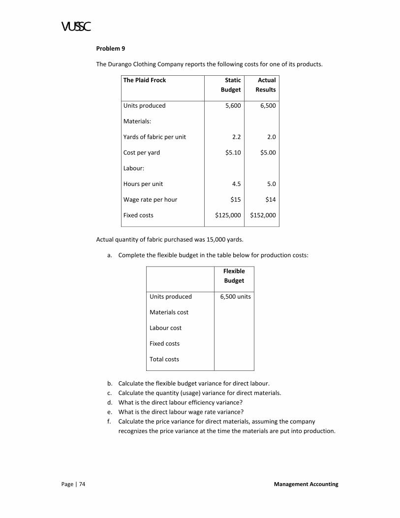
Page | 74 Management Accounting
Problem 9
The Durango Clothing Company reports the following costs for one of its products.
The Plaid Frock Static
Budget
Actual
Results
Units produced
Materials:
Yards of fabric per unit
Cost per yard
Labour:
Hours per unit
Wage rate per hour
Fixed costs
5,600
2.2
$5.10
4.5
$15
$125,000
6,500
2.0
$5.00
5.0
$14
$152,000
Actual quantity of fabric purchased was 15,000 yards.
a. Complete the flexible budget in the table below for production costs:
Flexible
Budget
Units produced
Materials cost
Labour cost
Fixed costs
Total costs
6,500 units
b. Calculate the flexible budget variance for direct labour.
c. Calculate the quantity (usage) variance for direct materials.
d. What is the direct labour efficiency variance?
e. What is the direct labour wage rate variance?
f. Calculate the price variance for direct materials, assuming the company
recognizes the price variance at the time the materials are put into production.

Management Accounting Page | 75
Problem 10
Arden Brothers reports the following cost information for one of its products.
Product Model XJ‐12 Static
Budget
Actual
Results
Units produced
Materials:
Pounds of materials per unit
Cost per pound of materials
Labour:
Hours per unit
Wage rate per hour
Fixed costs
900
3
$7.00
1.0
$13
$45,000
850
4
$6.50
1.2
$10
$39,000
Actual quantity of materials purchased was 4,000 pounds.
a. Calculate the flexible budget variance for direct labour.
b. Calculate the price variance for direct materials, assuming the company
recognizes the price variance at the time the materials are purchased.
c. Calculate the quantity (usage) variance for direct materials.
d. What is the direct labour wage rate variance?
e. What is the direct labour efficiency variance?
Problem 11
The Oswald Company makes four products in its factory in Jefferson City. Following is
production and cost information for April:
Steppers Runners Walkers Gliders
Actual Results
Units produced
Machine hours per unit
Budget
Units produced
Machine hours per unit
80
7
100
8
70
7
70
8
60
6
50
7
50
5
50
5

Page | 76 Management Accounting
Oswald allocates variable overhead using machine hours. Actual variable overhead was
$456,789. Budgeted variable overhead was $654,321.
a. Calculate the variable overhead spending and efficiency variances for steppers.
Be sure to indicate if these variances are favourable or unfavourable.
Problem 12
Preparation of a box of Chex Party Mix is budgeted to require 1.0 pound of Wheat Chex,
1.5 pounds of Rice Chex, and 0.8 pounds of Corn Chex. On Tuesday, the manager’s five‐
year‐old son sat at the control panel of the highly‐automated factory and made 50
boxes of Party Mix. The following information pertains to material variances for that
day's production, analysed by ingredient:
Wheat Chex Rice Chex Corn Chex
Price variance $16 Unfavourable $12 Favourable $19 Unfavourable
Usage variance $20 Unfavourable $25 Favourable $10 Favourable
The actual prices were $0.30 more per pound of Wheat Chex, $0.20 less per pound of
Rice Chex, and $0.50 more per pound of Corn Chex, than their standard prices.
a. Determine the standard price per pound of each ingredient.
b. Determine the number of pounds used of each ingredient.
Problem 13
Billy Bones, your long‐time business partner in the rum‐making business, dies
unexpectedly from natural causes. (It’s unexpected because nobody expected Billy to
live long enough to die from natural causes.) You now discover that he was not always
so honest in his business dealings, and the company’s silent partners are becoming not‐
so‐silent about the return on their investment. The silent partners demand to know the
company’s revenue for the year just ended.
You know that the financial statements that Billy prepared before his death were a
hoax. But you also know that the company’s rum recipe calls for one barrel of molasses
to produce 20 pints of rum, and that the company had no beginning or ending inventory
of either molasses or rum. Also, you find among Billy’s private papers the following
information, which you believe is reliable. The company’s fixed costs are $2,530 per
year. The company budgeted $2 per barrel of molasses, but paid $0.10 more per barrel
of molasses than budgeted, resulting in an unfavourable price variance for molasses of
$115 for the year. Also, the company had an unfavourable quantity variance for
molasses of $74 for the year. (Somehow, under Billy’s supervision, all variances were
always negative.) Also, a few days before he died, Billy scribbled a note to himself that
at the sales price that the company has had in place for over two years now, and at the
current variable cost per pint of $0.30 (which includes molasses and all other variable
costs), the company’s breakeven volume was 11,500 pints of rum.

Management Accounting Page | 77
a. How many pints of rum were produced and sold during the year?
b. Calculate the company’s revenue for the year.
LESSON SUMMARY
The cost of labour and the price of materials can be impacted by a number of different
variables. Entrepreneurs need to understand how to calculate variance and to make
adjustments to their budgets based on their financial analysis.

Page | 78 Management Accounting
UNIT 2 – SUMMARY
SUMMARY
Understanding the foundation of management accounting is the first step in mastering
the concepts and methods of successfully operating your business in a financially
responsible way. You must understand the factors that impact costs including direct
costs for materials and labour. You must recognize the difference between cost,
volume and profit and the impact of flexible budgeting vs. standard budgeting.
NEXT STEPS
In the next unit we will continue to build on this foundation. We will continue to
explore product cost and how to effectively allocate costs. As you can see the principles
related to costing are an essential part of the managing your accounts.

Management Accounting Page | 79
UNIT 3: PRODUCT COSTING AND COST ALLOCATIONS
UNIT INTRODUCTION
A cost is an expense (usually monetary) that needs to be undertaken to exchange,
consume or create products or procure services. When operating a business different
costs are needed for different purposes. We need to understand product costing and
how to allocate costs so that we can better manage our business.
When incurred, costs are initially reviewed and accumulated by some classification
system. Costs with one or more characteristics in common may be accumulated into
cost pools. Costs are then reassigned, differently for specified purposes, from these cost
pools to one or more cost objects.
In this unit we will examine different costing methods and how to allocate these costs in
way that most benefits the business.
UNIT OBJECTIVES
Upon completion of this unit you will be able to:
1. Employ the following costing models:
a. Product Costing.
b. Normal Costing.
c. Standard Costing.
d. Activity‐Based Costing.
2. Allocate service department costs.
3. Explain the role of cost in setting prices.
4. Establish prices for products and services.
UNIT READINGS
As you complete this unit you are required to read the following Lessons/articles:
<To be provided by your instructor>.
ASSIGNMENTS AND ACTIVITIES
Complete the lesson exercises and problems at the end of each lesson before
proceeding to the next lesson.

Page | 80 Management Accounting
LESSON 3.1: PRODUCT COSTING
LESSON INTRODUCTION
Product costing is a methodology associated with managerial accounting, i.e.,
accounting intended to serve management in an operational context rather than to
measure organizational performance. Product costing is intended accurately to
determine the cost of a unit of production (or of a service delivered) by study of every
resource used in its creation.
LESSON OBJECTIVES
Upon completion of this lesson you will be able to:
1. Explain product costing and cost objects.
2. Identify direct costs and overhead costs.
3. Describe cost allocation bases and overhead rates.
WHAT IS PRODUCT COSTING?
Product costing evolved in an environment of mass production in the second half of the
20th century as ever more managerial attention was focused on optimizing the
production function. Traditional financial accounting approaches have been—and
continue to be—based on measurements of fairly rough granularity. For determining
corporate profitability, it is sufficient generally to track raw materials, labor, tooling,
and energy inputs and to sum these into production costs. Pricing of different products,
of course, necessitated finer distinctions so that costs associated with classes of
products would be available as a basis for differential pricing. Closer attention to the
costs of, for instance, low‐, medium‐, and high‐end models of a vehicle or a device then
proliferated "downward." The costing of composite products required costing of their
components. In turn operations on each component might vary. Some might require
more or less strength and hence heavier forgings; these in turn might need more or less
additional machining. Some components could be attached mechanically, others had to
be welded. These operations could be measured in time, time in dollars. A systematic
analysis of how a product came to be, the inputs cost as received and then the
operations performed on them individually estimated, produced the final cost of
production from which receipts from sale of scrap would be deducted to get a net cost.
Product costing evolved further from this point by assigning an appropriate percentage
of total overhead and also measuring additional costs upstream—such as packaging,
warehousing, and delivery to the ultimate buyer.
The analytical resources made available by such detailed information have made
product costing a routine aspect of most significantly‐sized manufacturing operations.
Product costing data act as feedback to designers, are used in manufacturing
management to identify ideal workflow, influence the purchase of tooling, and are used
in precise pricing of goods. Product costing is used in most routine production activities,
including service occupations, although the level of detail sought is variable and usually
determined by the size of the operation. Even in quite small businesses, some level of

Management Accounting Page | 81
product costing is practiced in that managements usually know the costs associated
with important functions identified with different products.
SOME USEFUL DEFINITIONS
To understand product costing you must understand some specific terms. Review the
terms below.
Cost Object: A cost object is anything that we want to know the cost of. We might
want to know the cost of making one unit of product, or a batch of product, or all of
Tuesday’s production, in which case the cost objects are one unit of product, a batch
of product, or Tuesday’s production, respectively. We might want to know the cost
of operating a department or a factory, in which case the cost object is the
department or factory. In a service sector company, we might want to know the cost
of treating a patient in a hospital, or the cost of conducting an audit, in which case
the cost object is the patient or the audit client. In a government setting, a cost
object might be a program such as “Meals on Wheels.”
Product Costs: A product cost is any cost that is associated with units of product for
a particular purpose. Hence, the identification of product costs depends on the
purpose for which it is done. For example, the factory manager is interested in
manufacturing costs, whereas the merchandising manager might be interested in
both manufacturing and nonmanufacturing costs, including research and
development, marketing, and advertising costs.
Inventory Related Costs: These are costs that are debited to inventory for either
external or internal reporting purposes. For manufacturing firms, all Inventory
Related costs are manufacturing costs, but the reverse is not necessarily true. In
other words, Inventory Related costs are either the complete set or a subset of
manufacturing costs, and non‐manufacturing costs are never included as Inventory
Related costs. For merchandising firms, Inventory Related cost is usually the
purchase price of inventory.
Period Costs: These are costs that are expensed when incurred, usually because
they are not associated with the manufacture of products. Examples include
advertising costs and research and development costs. Period costs are
distinguished from Inventory Related costs.
Direct Costs and Overhead Costs: In relation to a given cost object, all costs are
either direct costs or overhead costs. Direct costs can be traced to the cost object in
an economically feasible way. Overhead costs (also called indirect costs) are
associated with the cost object, but cannot be traced to the cost object in an
economically feasible way. These terms apply to companies in all sectors of the
economy and to all types of organizations.
Cost Driver: A cost driver is any factor that affects costs. A change in the cost driver
will cause a change in the total cost of a related cost object. Any one cost object
Page | 82 Management Accounting
almost always has numerous cost drivers. This term applies to companies in all
sectors of the economy and to all types of organizations.
Cost Allocation: The assignment of overhead costs to the cost object. This term
applies to companies in all sectors of the economy and to all types of organizations.
Cost Allocation Base: A quantitative characteristic shared by multiple cost objects
that is used to allocate overhead costs among the cost objects. A cost allocation
base can be a financial measure (such as the raw material cost of each unit of
product) or a nonfinancial measure (such as direct labour hours incurred in the
manufacture of each unit of product). The simplest cost allocation base is simply the
number of cost objects (e.g., the number of units produced by the factory during a
period of time).
The distinction between a cost driver and a cost allocation base can be summarized
as follows. A cost driver is an economic concept; it relates to the economic reality of
the business. A cost allocation base is an accounting choice that is made by
accountants and managers. Usually, the best choice for a cost allocation base is a
cost driver.
Conversion Costs: All manufacturing costs other than direct materials.
OVERVIEW OF PRODUCT COSTING
Product costing follows these five basic steps:
1. Identify the cost object;
2. Identify the direct costs associated with the cost object;
3. Identify the overhead costs;
4. Select the cost allocation base to use in assigning overhead costs to the cost
object;
5. Develop the overhead rate for allocating overhead to the cost object.
The cost accounting system “builds up” the cost of product (or other cost object) by
recording to a job cost sheet, a work‐in‐process account, or some other appropriate
ledger, the direct costs that can be traced to the product, and a share of the overhead
costs, which are allocated to the product by multiplying the overhead rate by the
amount of the allocation base identified with the cost object.
COST OBJECTS
Recall that a cost object is anything that we want to know the cost of, such as a product
or service.
There is a common convention that can be confusing. We often talk about the cost
object (the thing we want to know the cost of) as one unit of product, because factory
managers and product managers speak in terms of unit costs. These managers want to
know the unit cost for product pricing, product sourcing, and performance evaluation
purposes. They do not want to talk about the cost of making 620 units, even if that is
the batch size. However, in most batch processes, there would be very little benefit and

Management Accounting Page | 83
enormous additional expense in determining the cost of each unit of product
individually. Rather, the accounting system treats the batch as the cost object, and to
derive a unit cost, we divide the cost of the batch by the number of units in the batch.
Hence, loosely speaking, we talk as if a unit of product is the cost object, but more
precisely, it is the batch (or the production run in an assembly‐line process, or perhaps
one day’s production in a continuous manufacturing process) that constitutes the cost
object.
DIRECT COSTS
Management accounting classifies product costs as either direct costs or overhead costs
(indirect costs). This distinction is important because costing systems handle these two
types of costs very differently. The distinction is sometimes subtle, because whether a
cost is direct or overhead is a function of the cost object, and also partly a matter of
choice on the part of managers and accountants.
Following are three definitions of direct costs from different accounting textbooks:
Direct costs of a cost object are costs that are related to the cost object and can
be traced to it in an economically feasible way.
Direct costs are costs that can be directly attached to the unit under
consideration.
Direct costs are costs that can be traced easily to specific products.
Direct costs are also called prime costs. For manufacturing companies, direct costs
usually can be categorized as either materials or labour.
Direct Materials: materials that become part of the finished product and that can be
conveniently and economically traced to specific units (or batches) or product.
An example of direct materials for an apparel manufacturer is fabric. All other materials,
such as thread and zippers, are probably indirect.
Direct Labour: costs for labour that can be conveniently and economically traced to a
unit (or batch) of product. The following examples show how the determination of
whether a cost is direct or overhead depends on the identification of the cost object:
Examples of Direct Labour for an Apparel Manufacturer
If the cost object is a single pair of pants, in a batch of several dozen pairs:
Most likely no labour is direct.
If the cost object is a batch of several dozen pairs of pants:
Most likely sewing operators’ wages are direct.
If the cost object is a production line in the factory:

Page | 84 Management Accounting
Add the line manager’s salary, and possibly wages incurred in the cutting room
(where rolls of fabric are cut into panels and pieces that are then sewn together).
If the cost object is the entire factory:
Add the factory manager’s salary, wages of maintenance and janitorial workers, and
salaries of front office personnel.
Even though it is likely that no labour is direct with respect to a single pair of pants, if
labour is direct with respect to a batch of 50 or 100 units, cost accountants would
usually (and loosely) call labour a direct cost with respect to units of product, and divide
the direct labour cost for the batch by the number of units per batch to derive the
direct labour cost per unit.
OVERHEAD COSTS
Overhead costs are costs that are related to the cost object, but cannot be traced to the
cost object in an economically feasible way. Overhead costs are not directly traceable to
specific units of production. Examples of overhead costs incurred at an apparel
manufacturer, when the cost object is a batch of product, would usually include the
following:
Electricity
Factory office salaries
Building and machine maintenance
Factory depreciation
The distinction between direct costs and overhead costs relate, in some measure, to the
way the accounting system treats the cost. For example, one apparel manufacturer
might track thread using the same methods that are used to track fabric, thus treating
thread as a direct material. Another apparel manufacturer might decide that the cost of
thread is immaterial, and does not warrant the cost and effort to track it as a direct
cost. For this company, thread is an overhead cost. Therefore, whether some costs are
direct or overhead depend on a choice made by the manager and the cost accountant.
There are three ways overhead costs can be treated in any decision‐making context:
1. they can be ignored,
2. they can be treated as a lump‐sum, or
3. they can be allocated to the products and services (i.e., to the cost objects) to
which they relate.
Each of these three alternatives is appropriate, depending on the circumstances and the
purpose for which the accounting is done. However, in this Lesson and throughout
much of this book, we are concerned with the third alternative: how to allocate
overhead costs to products and services.

Management Accounting Page | 85
COST ALLOCATION BASES
The allocation base is the “link” that is used to attach overhead costs to the cost object.
In a manufacturing setting, the simplest allocation base is the number of units
produced. For example, if the factory makes 15,000 units, the accounting system can
simply “spread” the overhead costs evenly over all 15,000 units. The problem with using
units as an allocation base, however, is that if the factory makes a range of different
products, those products might differ significantly in their resource utilization. A deluxe
widget might require twice as much labour and 20% more materials than a standard
widget, and one might infer that the deluxe widget also requires more resources that
are represented by overhead costs.
Whatever cost allocation base is chosen, it must be a “common denominator” across all
cost objects. For example, a furniture factory could allocate overhead costs across all
products using direct labour hours, because direct labour is incurred by all products
made at the factory. However, it would not seem appropriate to allocate factory
overhead based on the quantity of wood used in each unit, if the factory makes both
wood furniture and a line of plastic‐moulded, because no overhead would be allocated
to the plastic chairs.
OVERHEAD RATES
The overhead rate is the ratio of cost pool overhead dollars in the numerator, and the
total quantity of the allocation base in the denominator:
The result represents dollars of overhead per unit of the allocation base. For example, if
an apparel factory allocates overhead based on direct labour hours, the overhead rate
represents dollars of overhead per direct labour hour. Assume the overhead rate is $20
per direct labour hour. Then for every hour that a sewing operator spends working on
product, $20 will be allocated to the products that the sewing operator assembles
during that hour.
EXAMPLE OF ACTUAL COSTING ‐ ZFN APPAREL COMPANY,
The ZFN apparel company in Albuquerque, New Mexico makes jeans and premium
chinos. Each product line has its own assembly line on the factory floor. Overhead costs
for the factory for 2005 were $3,300,000. 500,000 jeans and 400,000 chinos were
produced during the year. 500,000 direct labour hours were used: 200,000 for jeans,
and 300,000 for chinos. The average direct labour wage rate was the same on both
assembly lines, and was $14 per hour. Denim fabric is used to make jeans, and chinos
are made from a cotton twill fabric. Overhead is allocated using direct labour hours.

Page | 86 Management Accounting
The following journal entries and T‐accounts illustrate how the accounting system
records the manufacturing activities of the factory in order to derive product cost
information for jeans and chinos. Journal entry (6) to debit overhead to work‐in‐process
is based on an overhead rate calculated as follows.
$3,300,000 ÷ 500,000 direct labour hours = $6.60 per direct labour hour.
In practice, the factory would track costs by batch, or perhaps weekly, but to simplify
our example, we record only one journal entry for each type of transaction. We also
make the unrealistic assumption that there is no work‐in‐process at the end of the
period. To focus the presentation on inventory‐related accounts, T‐accounts for some
non‐inventory accounts, and the entry to debit accounts receivable and credit revenue,
are omitted.
(1) Raw Materials: denim fabric $3,000,000
Raw Materials: cotton twill 2,250,000
Accounts Payable $5,250,000
(To record the purchase of 600,000 yards of denim fabric at $5.00 per yard, and 500,000
yards of cotton twill fabric at $4.50 per yard.)
(2) Work‐in‐process: Jeans $2,500,000
Raw Materials: denim fabric $2,500,000
(To record materials requisitions for 500,000 yards, for the movement of denim from
the receiving department to the cutting room.)
(3) Work‐in‐process: Chinos $2,160,000
Raw Materials: cotton twill $2,160,000
(To record materials requisitions for 480,000 yards, for the movement of cotton twill
from the receiving department to the cutting room.)
(4) Work‐in‐process: Jeans $2,800,000
Work‐in‐process: Chinos 4,200,000
Accrued Sewing Operator Wages $7,000,000
(To record sewing operator wages for the year: 200,000 hours for jeans, and 300,000
hours for chinos, at $14 per hour.)
(5) Factory Overhead $3,300,000
Accounts Payable $1,800,000
Accrued Wages for Indirect Labour 900,000

Management Accounting Page | 87
Accumulated Depreciation 600,000
(To record overhead costs incurred during the year, including utilities, depreciation,
repairs and maintenance, and indirect wages and salaries.)
(6) Work‐in‐process: Jeans $1,320,000
Work‐in‐process: Chinos 1,980,000
Factory Overhead $3,300,000
(To allocate factory overhead to production, using an overhead rate of $6.60 per direct
labour hour.)
(7) Finished Goods: Jeans $6,620,000
Work‐in‐process: Jeans $6,620,000
(To record the completion of all 500,000 jeans, at $13.24 per pair.)
(8) Finished Goods: Chinos $8,340,000
Work‐in‐process: Chinos $8,340,000
(To record the completion of all 400,000 chinos, at $20.85 per pair.)
(9) Cost of Goods Sold: Jeans $5,296,000
Cost of Goods Sold: Chinos 7,297,500
Finished Goods: Jeans $5,296,000
Finished Goods: Chinos 7,297,500
(To record the sale of 400,000 jeans and 350,000 chinos.)
Raw Materials:Denim Fabric
Raw Materials: Cotton Twill
(1) $3,000,000 $ 500,000
$2,500,000
(2) (1) $2,250,000
$ 90,000
$2,160,000 (3)
Accrued Sewing Operator Wages
Factory Overhead
$7,000,000
(4) (5) $3,300,000
$0
$3,300,000 (6)

Page | 88 Management Accounting
Work‐in‐Process: Jeans
Work‐in‐Process: Chinos
(2) (4) (6)
$2,500,000 2,800,000 1,320,000
$0
$6,620,000
(7) (3)(4)(6)
$2,160,0004,200,0001,980,000
$0
$8,340,000 (8)
Finished Goods: Jeans
Finished Goods: Chinos
(7) $6,620,000 $1,324,000
$5,296,000
(9) (8) $8,340,000 $1,042,500
$7,297,500 (9)
Cost of Goods Sold: Jeans
Cost of Goods Sold: Chinos
(9) $5,296,000
(9) $7,297,500
Accounts Payable
$5,250,0001,800,000
(1) (5)
The per‐unit inventory cost is calculated as follows:
Jeans: $6,620,000 ÷ 500,000 pairs = $13.24 per pair
Chinos: $8,340,000 ÷ 400,000 pairs = $20.85 per pair

Management Accounting Page | 89
These amounts, which are used in journal entry (9), can be detailed as follows:
Input Jeans Chinos
Fabric
Direct labour
Overhead
Total
1 yard/jean x $5/yard = $5.00
0.4 hrs/jean x $14/hr = $5.60
0.4 hrs/jean x $6.60/hr = $2.64
$13.24
1.2 yards/chino x $4.50/yard = $5.40
0.75 hrs/chino x $14/hr = $10.50
0.75 hrs/chino x $6.60/hr = $4.95
$20.85
In the above table, the direct labour hours per jean and per chino appear in the lines for
both the per‐unit direct labour cost and the per‐unit overhead cost, because overhead
is allocated based on direct labour hours. If the allocation base had been something
else, such as machine hours, the hours per unit would only appear in the calculation of
the direct labour cost.
More overhead is allocated to each pair of chinos than to each pair of pants ($4.95
versus $2.64) because direct labour hours has been chosen as the allocation base, and
each chino requires more direct labour time than each pair of jeans (0.75 hours versus
0.40 hours). Changing the allocation base cannot change the total amount of overhead
incurred, but it will usually shift costs from some products to others. For example, if the
allocation base were units of production instead of direct labour hours, the overhead
rate would be:
$3,300,000 ÷ 900,000 units = $3.67 per unit.
In this case, the total cost per pair of jeans would increase from $13.24 to $14.27, and
the total cost per pair of chinos would decrease from $20.85 to $19.57.
Because the choice of allocation base determines how overhead is allocated across
products, product managers usually have preferences over this choice (because a lower
reported product cost results in higher reported product profitability). However, the
company’s choice of allocation base should be guided, if possible, by the cause‐and‐
effect relationship between activity on the factory floor and the incurrence of overhead
resources. For example, direct labour hours is a sensible allocation base if the significant
components of overhead increase as direct labour hours increase. More direct labour
implies more indirect labour by human resources and accounting personnel, janitorial
staff and other support staff. Also, more direct labour implies more machine time,
which implies more electricity usage, and more repairs and maintenance expense. For
these reasons, direct labour hours are probably a better choice of allocation base than
units of product.

Page | 90 Management Accounting
LESSON PROBLEMS
Now review the following problems and answer the related questions. Record your
answers in your course workbook.
Problem 1
A company allocates overhead based on direct labour cost (dollars). The rate is 160% of
the direct labour cost. A job has direct materials cost of $12,000 and direct labour cost
of $14,000 (700 labour hours). What is the total cost of the job?
a. $26,000
b. $34,400
c. $48,400
d. $27,120
Problem 2
A multi‐product manufacturing company uses many different machines and employs a
labour force with widely‐varying skill levels and pay rates. Generally, the higher paid
and more skilled employees operate the more complex and expensive machinery. If all
overhead is going to be applied using a single overhead rate, based on the information
provided, which allocation base would work best in this environment?
a. Machine hours
b. Direct labour hours
c. Direct labour dollars
d. Direct material dollars
Problem 3
The Quad City Candy Company uses a budgeted overhead rate, and allocates variable
overhead based on direct material costs (i.e., direct materials dollars). The company
only allocates variable overhead; the company does not allocate fixed overhead.
Following is information for the year 2005:
Budget Actual
Boxes of candy (this is output)
Variable overhead
Fixed overhead
Direct labour:
Hours per box
Hourly wage rate
10,000
$20,000
$10,000
0.5
$10
11,000
$22,000
$13,200
0.4
$12

Management Accounting Page | 91
Budget Actual
Direct materials:
Pounds per box
Cost per pound
2
$5
2
$4
a. Calculate the overhead rate for applying overhead:
Problem 4
The Santa Fe Candy Company expects to incur overhead of $60,000. Also, the company
expects to incur 300 direct labour hours (which is paid an average of $20 per hour) and
200 machine hours, in order to produce 30,000 pounds of candy.
a. Using the information provided, calculate four different overhead rates using
four different allocation bases. In each case, be sure to identify the allocation
base.
Problem 5
The Bernalillo factory of Winrock and Associates makes two models of a portable
pneumatic compressor: Model #A567 and Model #B234. Information about the year
1967 follows:
Model
#A567
Model
#B234
Units produced
Direct materials costs
Direct labour hours
500
$40,000
5,000
500
$60,000
5,000
Factory overhead for the year was $180,000. The average wage rate for workers on the
Model #A567 production line is $10 per hour. The average wage rate for workers on the
Model #B234 production line is $20 per hour.
a. Assume the company allocates overhead based on direct labour hours. What is
the overhead rate?
b. What is the total cost per unit for the Model #B234?
c. Assume the company changes the allocation base from direct labour hours to
direct labour costs (i.e., direct labour dollars). What is the new overhead rate?
d. Using this new overhead rate, what is the new cost per unit for the Model
#B234?
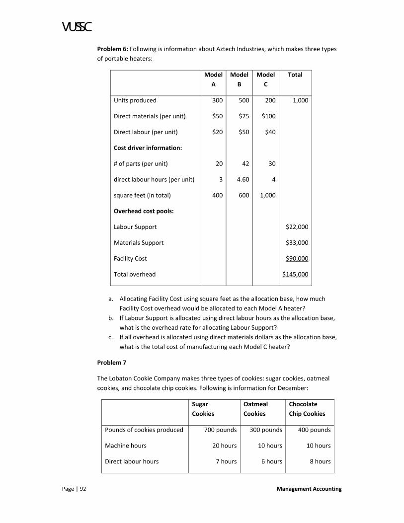
Page | 92 Management Accounting
Problem 6: Following is information about Aztech Industries, which makes three types
of portable heaters:
Model
A
Model
B
Model
C
Total
Units produced
Direct materials (per unit)
Direct labour (per unit)
Cost driver information:
# of parts (per unit)
direct labour hours (per unit)
square feet (in total)
Overhead cost pools:
Labour Support
Materials Support
Facility Cost
Total overhead
300
$50
$20
20
3
400
500
$75
$50
42
4.60
600
200
$100
$40
30
4
1,000
1,000
$22,000
$33,000
$90,000
$145,000
a. Allocating Facility Cost using square feet as the allocation base, how much
Facility Cost overhead would be allocated to each Model A heater?
b. If Labour Support is allocated using direct labour hours as the allocation base,
what is the overhead rate for allocating Labour Support?
c. If all overhead is allocated using direct materials dollars as the allocation base,
what is the total cost of manufacturing each Model C heater?
Problem 7
The Lobaton Cookie Company makes three types of cookies: sugar cookies, oatmeal
cookies, and chocolate chip cookies. Following is information for December:
Sugar
Cookies
Oatmeal
Cookies
Chocolate
Chip Cookies
Pounds of cookies produced
Machine hours
Direct labour hours
700 pounds
20 hours
7 hours
300 pounds
10 hours
6 hours
400 pounds
10 hours
8 hours

Management Accounting Page | 93
Sugar
Cookies
Oatmeal
Cookies
Chocolate
Chip Cookies
Average wage per hour $10 per hour $12 per hour $9 per hour
Total overhead incurred in December was $8,400.
a. Calculate the overhead applied per pound of Oatmeal Cookies, when all
overhead is applied using machine hours as the allocation base.
b. Now assume that $4,000 of the overhead is fixed, and the remainder is variable.
Calculate the overhead applied per pound of Sugar Cookies, using machine
hours to allocate fixed overhead and direct labour dollars to allocate variable
overhead.
Problem 8
The Svendsgaard Organic Cereal Company makes 20 brands of cereal, including wheat
squares, corn squares, and rice squares. Following is information for December:
Wheat
Squares
Corn
Squares
Rice
Squares
Pounds of cereal produced
Machine hours
Direct labour hours
800 pounds
40 hours
45 hours
600 pounds
30 hours
60 hours
500 pounds
30 hours
40 hours
Total overhead incurred in December was $10,000. Total machine hours incurred were
500.
a. Calculate the overhead rate using machine hours as the allocation base.
b. Calculate the overhead applied per pound of corn squares using machine hours
as the allocation base.
Problem 9
Teddy Bear Fudge Company makes two types of fudge: plain fudge and fudge with nuts.
Following is information for operations in the month of February. All quantities are
expressed in pounds. There is no direct labour.
Total Plain
Fudge
Fudge with
Nuts
Beginning inventory
Production
0
1,000
0
600
0
400

Page | 94 Management Accounting
Total Plain
Fudge
Fudge with
Nuts
Sales
Per unit information:
Sales price per pound
Direct materials
Sales commission
Variable manufacturing overhead
Fixed costs:
Fixed manufacturing overhead
Fixed non‐manufacturing overhead
850
$500
$2,000
$300
500
$8.00
$2.00
$0.50
350
$8.00
$2.25
$0.50
1. What is the manufacturing cost for each type of fudge, assuming the company
allocates overhead based on direct materials dollars?
LESSON SUMMARY
Product costing takes place before all of the work is actually accomplished. In a business
good estimating is the difference between turning a profit or booking a loss. But the
principles that apply are identical. Both in the services and in the manufacturing
environments, accurate costing (hence pricing) will depend on subdividing the work
carefully into its many categories, measuring time and purchased materials and
services. In the next lesson we will examine a second type of costing: normal costing.

Management Accounting Page | 95
LESSON 3.2: NORMAL COSTING
LESSON INTRODUCTION
Normal costing is used to derive the cost of a product. It includes the following
components: the actual cost of materials; the actual cost of labor; and a standard
overhead rate that is applied using the product's actual usage of whatever allocation
base is being used (such as direct labor hours or machine time).
LESSON OBJECTIVES
Upon completion of this lesson you will be able to:
1. Explain normal costing and its application in business.
2. Describe the advantages of using budgeted overhead rates.
3. Calculate overhead rates.
NORMAL COSTING
Many companies calculate and apply this overhead rate using, not actual overhead
costs and the actual quantity of the allocation base, but rather budgeted overhead costs
and the budgeted quantity of the allocation base. When a company uses budgeted
overhead rates in its costing system, but all other information in the costing system is
based on actual costs, the company is using what is called a normal costing system.
It is important to remember that although there are no rules in management
accounting, companies always, as a matter of practice, use either budgeted numbers in
both the numerator and the denominator of the overhead rate, or actual numbers in
both the numerator and the denominator of the overhead rate. Companies never use
budgeted overhead divided by the actual quantity of the allocation base, or actual
overhead divided by the budgeted quantity of the allocation base.
It is also important to remember that in a normal costing system, the budgeted
overhead rate is multiplied by the actual quantity of the allocation base incurred. In
Lesson 10, we will discuss another type of accounting system, called a standard costing
system that multiplies the budgeted overhead rate by a flexible budget quantity for the
allocation base: the amount of the allocation base that should have been used for the
amount of output achieved. However, in a normal costing system, the only budgeted
number is the overhead rate; direct costs are recorded at their actual cost, and the
overhead rate is multiplied by the actual quantity of the allocation base used during the
period.
ADVANTAGES OF USING BUDGETED OVERHEAD RATES
There are three principal reasons that many companies in all sectors of the economy
use budgeted overhead rates, either as part of a normal costing system or as part of a
standard costing system.
1. Actual overhead rates are not known in a timely manner: Factory managers
often use production cost information in their monitoring of the manufacturing
process. Control of manufacturing activities is a daily or weekly process, not a

Page | 96 Management Accounting
monthly or quarterly process. The challenge of collecting and reporting actual
direct costs—the cost of materials and labour used in production—within one
or two days of actual production is difficult, but increasingly possible. For
example, all materials used in production have already been purchased, and the
cost of those materials can be ascertained. Also, sophisticated data collection
systems, often called real‐time systems, can track the movement of inventory,
and track labour resources incurred at various work stations, as production
occurs. Even the quantity of the overhead cost allocation base used in
production can probably be ascertained, because the allocation base is usually a
measure of a direct input. However, many of the components that make up
overhead are not paid daily or even weekly. Utilities and property taxes are
often paid monthly or quarterly. The factory manager who wants to know the
cost of production on January 3 for the purpose of controlling operations on the
factory floor will not want to wait until the books are closed on January 31 for
that information. Usually, budgeted overhead rates are sufficiently close to
actual overhead rates so that normal costing systems provide reasonably
accurate cost information for management control purposes, and normal
costing can provide this information in a timely manner.
2. Overhead rates are subject to short‐run fluctuations: For an apparel factory in
El Paso, electric costs are significantly higher in July than in January due to the
cost of air conditioning. Should overhead rates be calculated and applied
separately for each month, or should overhead rates be averaged over the
entire year? The answer to this question is not clear, because it depends on the
types of decisions for which management will use factory cost information as an
input. For example, if the factory has excess capacity and management is
considering suspending factory operations for two weeks, monthly cost data
will assist in scheduling the down‐time to maximize cost savings (i.e., close the
factory for two weeks in July, not January). On the other hand, if several
product managers are scheduling production for the coming year, it would
seem counterproductive to provide these managers incentives to compete with
each other for January factory time, for the sake of obtaining the lower per‐unit
production cost, if some of them will have to schedule production in July in any
case. Using an overhead rate that averages over the entire year might be more
reasonable for production costing purposes like this one. In fact, many
companies prefer to average overhead rates over a quarter or an entire year,
and these companies usually prefer using budgeted overhead rates instead of
waiting until actual overhead is known at the end of the period.
3. When actual overhead rates are used, production volume of each product
affects the reported costs of all other products: This issue arises because the
production volume of each product affects the total quantity of the allocation
base in the denominator of the overhead rate, whereas an important
component of the numerator—fixed overhead—is invariant to changes in
production volume. Hence, as production volume of one product decreases

Management Accounting Page | 97
below budget, the overhead rate (which is common across all products)
increases, and when that overhead rate is applied to other products, those
products absorb more overhead (and so have higher reported costs) than was
budgeted. The important point here is that the direct costs and production
activity related to those other products could be exactly as planned, but the
reported costs of those products will be higher than planned, due entirely to
the production activities of another product. In a factory that makes jeans and
chinos, one might imagine the reaction of the jeans product manager when a
decline in chinos production increases the reported cost of each pair of jeans.
MISAPPLIED OVERHEAD
When budgeted overhead rates are used, it is very likely that the amount of overhead
applied to production (the debits to work‐in‐process) will differ from the actual
overhead incurred (credits to cash, accounts payable, and various other accounts)
during the period. This difference, which will occur whenever the budgeted overhead
rate differs from the actual overhead rate, is called misapplied overhead. If less
overhead is applied to inventory than is actually incurred, then the difference is called
under applied overhead (it is also called under allocated overhead or under absorbed
overhead). If more overhead is applied to inventory than is actually incurred, then the
difference is called over applied overhead (it is also called over allocated overhead or
over absorbed overhead).
Mechanically, misapplied overhead is accumulated in one or more temporary accounts
that are closed out at the end of the period (month, quarter or year). These accounts
collect the misapplied overhead because when overhead is debited to inventory, the
corresponding credits are posted to these temporary accounts, and when overhead is
paid (or accrued), the corresponding debits are also posted to these temporary
accounts. The net difference between these debits and credits represents misapplied
overhead. If two temporary accounts are used, they are called something like
“overhead applied” and “overhead incurred.”
The nature of the closing entry to zero‐out these accounts depends on the materiality
of the misapplied overhead. If the amount is small, management might take the
expedient approach of closing out all misapplied overhead to a line‐item on the income
statement for the period. The misapplied overhead might be posted to cost‐of‐goods‐
sold, or might be treated as a period expense, but in either case, the effect is to increase
or decrease income by the total amount of misapplied overhead.
If the amount of misapplied overhead is material, management should consider
whether the entry to close out misapplied overhead should be made in such a way as to
approximate the balances in the balance sheet and income statement inventory
accounts that would have occurred had an actual costing system been used. If so, then
the entry to close out misapplied overhead should include the inventory balance sheet
accounts of work‐in‐process and finished goods inventory, as well as cost‐of‐goods‐sold
on the income statement. One technique that approximates this objective is to pro‐rate
misapplied overhead based on the ending balances in work‐in‐process, finished goods

Page | 98 Management Accounting
inventory, and cost‐of‐goods‐sold. A more accurate technique is to pro‐rate misapplied
overhead based on the amount of overhead in each of these three accounts.
If overhead is under applied, some managers close out the entire amount to the income
statement (thereby decreasing income) even if the amount is material. Conservatism is
often the justification for this approach.
EXAMPLE OF NORMAL COSTING ‐ ZFN APPAREL COMPANY
The ZFN apparel company in Albuquerque, New Mexico makes jeans and premium
chinos. Each product line has its own assembly line on the factory floor. Overhead costs
for the factory for 2005 were budgeted for $3,600,000, but came in below budget at
$3,300,000. Budgeted production for the year was 500,000 jeans and 500,000 chinos.
Actual production was 500,000 jeans and 400,000 chinos. The reduction in chinos
output relative to plan was due to unexpected slack in the demand for casual slacks.
The budgeted direct labour hours per jean is 0.5, and per chino is 0.7. In fact, 500,000
direct labour hours were used: 200,000 for jeans, and 300,000 for chinos. The average
direct labour wage rate was the same on both assembly lines, and was $14 per hour.
Denim fabric is used to make jeans, and chinos are made from a cotton twill fabric.
Overhead is allocated using direct labour hours.
The following journal entries and T‐accounts illustrate how a normal costing system
records the manufacturing activities of the factory in order to derive product cost
information for jeans and chinos.
The first five entries are identical to the ZFN example in the previous Lesson. The first
entry that differs as the result of using normal costing instead of actual costing is (6).
This entry to debit overhead to work‐in‐process is based on an overhead rate calculated
as:
Budgeted
Production
Budgeted hours per
unit
Budgeted
labour
hours
Jeans
Chinos
Total
500,000 units x
500,000 units x
0.5 hours per unit =
0.7 hours per unit =
250,000
350,000
600,000
The budgeted overhead rate = $3,600,000 ÷ 600,000 direct labour hours = $6.00 per
direct labour hour.
In practice, the factory would track costs by batch, or perhaps weekly, but to simplify
our example, we record only one journal entry for each type of transaction. We also
make the unrealistic assumption that there is no work‐in‐process at the end of the
period. To focus the presentation on inventory‐related accounts, T‐accounts for some
non‐inventory accounts are omitted. Many companies would use two separate

Management Accounting Page | 99
accounts instead of one account to track factory overhead; one account for factory
overhead incurred, and the other account for factory overhead allocated.
(1) Raw Materials: denim fabric $3,000,000
Raw Materials: cotton twill 2,250,000
Accounts Payable $5,250,000
(To record the purchase of 600,000 yards of denim fabric at $5.00 per yard, and 500,000
yards of cotton twill fabric at $4.50 per yard.)
(2) Work‐in‐process: Jeans $2,500,000
Raw Materials: denim fabric $2,500,000
(To record materials requisitions for 500,000 yards, for the movement of denim from
the receiving department to the cutting room.)
(3) Work‐in‐process: Chinos $2,160,000
Raw Materials: cotton twill $2,160,000
(To record materials requisitions for 480,000 yards, for the movement of cotton twill
from the receiving department to the cutting room.)
(4) Work‐in‐process: Jeans $2,800,000
Work‐in‐process: Chinos 4,200,000
Accrued Sewing Operator Wages $7,000,000
(To record sewing operator wages for the year: 200,000 hours for jeans, and 300,000
hours for chinos, at $14 per hour.)
(5) Factory Overhead $3,300,000
Accounts Payable $1,800,000
Accrued Wages for Indirect Labour 900,000
Accumulated Depreciation 600,000
(To record overhead costs incurred during the year.)
(6) Work‐in‐process: Jeans $1,200,000
Work‐in‐process: Chinos 1,800,000
Factory Overhead $3,000,000
(To allocate overhead to production, using a budgeted overhead rate of $6 per direct
labour hour, multiplied by actual hours used in production.)

Page | 100 Management Accounting
(7) Finished Goods: Jeans $6,500,000
Work‐in‐process: Jeans $6,500,000
(To record the completion of all 500,000 jeans, at $13.00 per pair.)
(8) Finished Goods: Chinos $8,160,000
Work‐in‐process: Chinos $8,160,000
(To record the completion of all 400,000 chinos, at $20.40 per pair.)
(9) Cost of Goods Sold: Jeans $5,200,000
Cost of Goods Sold: Chinos $7,140,000
Finished Goods: Jeans $5,200,000
Finished Goods: Chinos $7,140,000
(To record the sale of 400,000 jeans and 350,000 chinos.)
(10) Cost of Goods Sold: misapplied overhead $300,000
Factory Overhead $300,000
(To close out under applied overhead to COGS. The total amount is taken to COGS
because the result is not materially different from allocating misapplied overhead to
COGS and finished goods inventory)
Raw Materials: Denim Fabric
Raw Materials: Cotton Twill
(1) $3,000,000
500,000
$2,500,000 (2) (1) $2,250,000
90,000
$2,160,000 (3)
Accrued SewingOperator Wages
Factory Overhead
$7,000,000 (4) (5) $3,300,000
$0
$3,000,000
300,000
(6) (10)
Work‐in‐Process: Jeans Work‐in‐Process: Chinos
(2) (4) (6)
$2,500,000 2,800,000 1,200,000
$0
$6,500,000 (7) (3)(4)(6)
$2,160,000 4,200,000 1,800,000
$0
$8,160,000 (8)

Management Accounting Page | 101
Finished Goods: Jeans Finished Goods: Chinos
(7) $6,500,000 $1,300,000
$5,200,000
(9) (8) $8,160,000 $1,020,500
$7,140,000 (9)
Cost of Goods Sold: Jeans Cost of Goods Sold: Chinos
(9) $5,200,000
(9) $7,140,000
Accounts Payable COGS: misapplied overhead
$5,250,0001,800,000
(1)(5)
(10) $300,000
The per‐unit cost of finished goods inventory is calculated as follows:
Jeans: $6,500,000 ÷ 500,000 pairs = $13.00 per pair
Chinos: $8,160,000 ÷ 400,000 pairs = $20.40 per pair
These amounts can be detailed as follows:
Input Jeans Chinos
Fabric
Direct labour
Overhead
Total
1 yard/jean x $5/yard = $5.00
0.4 hrs/jean x $14/hr = $5.60
0.4 hrs/jean x $6.00/hr = $2.40
$13.00
1.2 yards/chino x $4.50/yard = $5.40
0.75 hrs/chino x $14/hr = $10.50
0.75 hrs/chino x $6.00/hr = $4.50
$20.40
Overhead is applied using the budgeted overhead rate of $6.00 per hour. However, this
budgeted overhead rate is multiplied by the actual direct labour hours used by each
product. Therefore, the only reason that more overhead or less overhead is allocated to
each unit of product than budgeted is because each product used more of the
allocation base or less of the allocation base (in this case, direct labour hours) than
planned. Jeans used less overhead per unit than planned (0.4 versus 0.5), so less
overhead is allocated to each pair of jeans than planned. Chinos used more overhead
than planned (0.75 versus 0.7), so more overhead is allocated to each pair of chinos
than planned.
The total misapplied overhead is a function of two factors: (1) the numerator in the
budgeted overhead rate differing from actual overhead incurred; and (2), the
denominator in the budgeted overhead rate differing from the actual quantity of the

Page | 102 Management Accounting
allocation base incurred. In the next two paragraphs, we consider each of these two
factors.
Less overhead was incurred than planned: $3,300,000 versus $3,600,000. It is probable
that one reason actual overhead incurred was less than budgeted is that fewer units
were produced than planned. Unless all overhead is fixed, a reduction in output should
decrease the total overhead incurred.
The denominator in the budgeted overhead rate can differ from the actual quantity of
the allocation base incurred for two reasons. First, the amount of the allocation base
used per unit of product (in this case, direct labour hours per unit) can differ from plan.
Jeans used less direct labour hours per unit than planned, but chinos used more direct
labour hours than plan. Second, the level of production can differ from plan (either total
production or product mix). Because fewer units were made than planned (900,000
units versus 1,000,000 units), less overhead was allocated than otherwise would have
been the case.
LESSON PROBLEMS
Now review the following problems and answer the related questions. Record your
answers in your course workbook.
Problem 1
A company uses a Normal Costing System, and allocated overhead using direct labour
hours. At the beginning of the year, the company estimated that there would be
$960,000 in overhead and 40,000 direct labour hours worked. At the end of the year,
the company had worked 39,000 hours and incurred $949,000 in overhead. What is the
under applied or over applied overhead for the year?
a. There is not enough information to determine this.
b. $13,000 under applied
c. $11,000 over applied
d. $11,000 under applied
Problem 2
DRG Company makes three products: cypress, silius, and sibelius. DRG expects to incur
$900,000 in overhead, and expects to use 300 machine hours to make 500 units of
cypress, 200 machine hours to make 100 units of silius, and 100 machine hours to make
50 units of sibelius. DRG uses a Normal Costing System, and uses machines hours as the
allocation base.
a. If DRG uses 50 machine hours to make 20 units of sibelius, and actually incurs
overhead of $1,111,000, how much overhead will be allocated to each unit of
sibelius?
b. If DRG uses 200 machine hours to make 400 units of cypress, 400 machine hours
to make 150 units of silius, and 50 machine hours to make 20 units of sibelius,
what is the amount of over applied or under applied overhead?

Management Accounting Page | 103
Problem 3
The not‐for‐profit health clinic Shots‐Я‐Us provides various types of vaccinations and
other shots, especially flu shots, to the public for free or for a nominal fee. The clinic is
funded by several local governmental agencies as well as by a number of charitable
organizations. Since different donors wish to fund different types of shots, the clinic
determines the full cost of each type of shot, by adding overhead to the direct costs,
and then provides this information to current and prospective donors.
Following are actual and budgeted costs for Shots‐Я‐Us for 2003:
Actual Budgeted
Number of patient visits
Number of shots administered
Fixed overhead: salaries, rent for the facility, insurance, depreciation.
Variable overhead: nursing staff hourly wages, utilities, disposable supplies.
Cost of hypodermics (a direct cost)
Cost of medications (a direct cost)
5,000
6,000
$94,000
$66,000
$1,000
$30,000
4,000
4,500
$110,000
$40,500
$750
$20,000
1. Under normal costing, the variable cost per shot is
a. $9 per shot
b. $13.61 per shot
c. $14.17 per shot
d. $38.06 per shot
2. Which of the following might help explain the increase in total variable overhead,
from budget to actual?
I. The increase in the number of shots given, from budget to actual.
II. A misclassification of some fixed costs as variable (i.e., the costs are actually
fixed, but are included under variable overhead, in both the budget and the
actual columns).
III. An increase in the average hourly wages for the nursing staff, from budget
to actual.
a. (I) only
b. (III) only
c. (I) and (III), but not (II)
d. (I), (II) and (III)

Page | 104 Management Accounting
Problem 4
The Santa Cruz Candy Company expects to incur overhead of $24,000. Also, the
company expects to incur 300 direct labour hours (which is paid an average of $10 per
hour) and 200 machine hours, in order to produce 2,000 pounds of candy.
a. Using the information provided, calculate three different overhead rates using
three different allocation bases. In each case, be sure to identify the allocation
base.
Problem 5
The Santa Cruz Machine Shop allocates overhead based on machine hours, using a
budgeted overhead rate. The budgeted overhead rate is calculated using an estimate of
6,000 machine hours in the denominator, and $60,000 in the numerator. Actual
overhead was $500 less than budgeted. Actual machine hours were 1,500 more than
budgeted. Calculate the misapplied overhead.
a. Indicate whether this misapplied overhead is under applied or over applied.
Problem 6
Following is information for Penquo, Inc., which makes crayons in its Billings, MT
factory:
Budget Actual
Production (# of boxes of crayons)
Total Direct Costs (materials & labour)
Total Machine Hours
Overhead (fixed and variable)
1,000
$ 2,000
140
$2,800
800
$ 2,400
100
$3,000
Penquo allocates overhead using a budgeted overhead rate, using machine hours as the
allocation base. The overhead rate is then applied to product based on actual machine
hours incurred. In other words, the company uses a Normal Costing system.
a. What is the overhead rate?
b. How much overhead would be applied to each box of crayons?
c. What is the actual direct cost of each box of crayons?
Problem 7
The Rio Grande Tile Company uses a budgeted overhead rate, and direct labour costs
(i.e., direct labour dollars) as the allocation base. Overhead is applied using actual
labour costs incurred. Following is information for January 2005. The labour wage rate

Management Accounting Page | 105
was budgeted at $6 per hour, but was actually $8 per hour. Overhead was budgeted at
$42,000, but was actually $49,000.
Ceramic
Tiles
Slate
Tiles
Total
Production:
Budgeted
Actual
Total Direct labour hours:
Budgeted
Actual
4,000
3,000
500
400
2,000
4,000
200
300
6,000
7,000
700
700
a. Calculate the overhead rate. How much overhead would be allocated to all
4,000 slate tiles?
b. Now assume the company uses a budgeted overhead rate, direct labour hours
as the allocation base, and applies overhead based on actual direct labour hours
incurred. How much overhead would be applied to each ceramic tile?
c. Now assume the company allocates overhead using direct labour hours as in
part B. What is the misapplied overhead? Is overhead over applied or under
applied?
Problem 8
The Svendsgaard Organic Cereal Company makes cereal. Following is information for
November:
Actual
Information
Budgeted
Information
Pounds of cereal produced
Total direct materials
Total direct labour
Total machine hours
Total direct labour hours
Total overhead
800 pounds
$3,200
$800
60 hours
45 hours
$30,000
800 pounds
$2,600
$800
50 hours
40 hours
$30,000
a. Calculate the overhead rate using Normal Costing and machine hours as the
allocation base.

Page | 106 Management Accounting
b. Using Normal Costing, how much overhead will be applied to each pound of
cereal?
c. Compute the amount of misapplied overhead.
Problem 9
Following is information for the James Woods Company, and one of the products made
by the company. The factory has the capacity to produce 1.5 million square feet of
wood product.
Budget for
the
Company
Actual for the
Company
Budget for
Mahogany
Laminate
Actual for
mahogany
Laminate
Production (in square feet) Direct Product Costs
Variable Overhead
Fixed Overhead
1,000,000
$2,500,000
$2,000,000
$1,500,000
1,200,000
$2,880,000
$2,400,000
$1,200,000
50,000
$150,000
40,000
$128,000
a. Calculate the amount of overhead allocated to all of the mahogany laminate if
the company uses a budgeted overhead rate, square feet of product as the
allocation base, and applies the overhead rate based on actual square feet
produced.
b. Calculate the amount of overhead allocated to all of the mahogany laminate if
the company uses a budgeted overhead rate, direct product cost as the
allocation base, and applies the overhead rate based on actual direct product
costs incurred.
c. Calculate the amount of overhead allocated to all of the mahogany laminate if
the company uses a budgeted overhead rate, square feet of product as the
allocation base, and applies the overhead rate based on actual square feet
produced. However, the company allocates variable overhead and fixed
overhead separately. The denominator for the overhead rate for variable
overhead is budgeted square feet, and the denominator for the overhead rate
for fixed overhead is factory capacity (in terms of square feet).
Problem 10
A factory makes jeans and chinos. Overhead was budgeted at $150,000, but was
actually $132,000. Budgeted production was 10,000 jeans and 5,000 chinos. Actual
production was 10,000 jeans and 2,000 chinos. Overhead is applied using a budgeted
overhead rate, and the allocation base is units of output.
a. Calculate the overhead rate.
b. How much overhead would be applied to the chinos production line?

Management Accounting Page | 107
c. What is the misapplied overhead? Is it under applied or over applied?
LESSON SUMMARY
In this lesson we explored a method of tracking production costs based on an
approximation of the prices of the inputs multiplied by the actual quantity of inputs
used. We discovered that normal costing, the actual prices are used for direct labour
and direct materials, and only the overhead rate is estimated. Extended normal costing
uses estimates for direct labour and direct material prices as well as overhead.
Selecting an accurate method of costing is important for maximizing profitability. Since
extended normal costing relies heavily on estimates of input prices, it may produce
inaccurate results unless estimates are carefully prepared. However, in cases where it is
very difficult to track all of the costs going into a product, extended normal costing may
be the most effective ways to assign production costs.
In the next lesson we examine another method of costing called standard costing.

Page | 108 Management Accounting
LESSON 3.3: STANDARD COSTING
LESSON INTRODUCTION
In this unit we are exploring a number of different costing models. One such accounting
process is call standard costing. Standard costing is the planned or expected costs used
for accounting for inventories and production. When actual costs differ from the
standard costs, variances are reported. We will explore the process of standard costing
in this lesson.
LESSON OBJECTIVES
Upon completion of this lesson you will be able to:
1. Define standards costs.
2. Describe standard costing systems.
3. Explain the relationship between standard costing systems and flexible
budgeting.
4. State the reasons for using a standard costing system.
5. Describe the similarities and differences between actual costing, normal costing
and standard costing.
OVERVIEW
If you were to design a cost accounting system with no accounting education other than
financial accounting courses, you would probably design an accounting system that
collects, summarizes, and reports actual costs. This approach would be consistent with
the implicit assumption throughout every financial accounting course that when
financial statements report historical cost data, such as would normally be the case for
cost‐of‐goods‐sold and ending inventory, that the information reported represents
actual costs. Therefore, it comes as a surprise to most students that the initial journal
entries to record the production and movement of inventory in the costing systems of
most manufacturing firms are not based on actual costs at all, but rather are based on
budgeted per‐unit costs.
In most manufacturing firms, the initial journal entries to debit work‐in‐process,
finished goods and cost‐of‐goods‐sold are based on the actual quantity of output
produced, multiplied by budgeted data about the inputs necessary to produce those
outputs, and the budgeted costs of those inputs. Then, at the end of the month (or
possibly quarterly), an “adjusting” or “closing” entry is made to record in the inventory
accounts the difference between actual costs incurred, and the budgeted information
that has formed the basis for the journal entries during the month. The nature of this
adjusting entry depends on the materiality of the amounts involved. If the differences
between actual costs and budgeted costs are small, this adjusting entry might be made
in an expedient manner, involving only cost‐of‐goods‐sold, but if the differences are
large, the adjusting entry might also involve work‐in‐process and finished goods
inventory accounts.
The accounting system described above is called a standard costing system, and it is
widely‐used by companies in the manufacturing sector of the economy. This Lesson

Management Accounting Page | 109
describes standard costing systems, and explains why companies use them. But first we
discuss a related concept, standard costs, which constitutes an important component of
standard costing systems.
STANDARD COSTS
A standard, as the term is usually used in management accounting, is a budgeted
amount for a single unit of output. A standard cost for one unit of output is the
budgeted production cost for that unit. Standard costs are calculated using engineering
estimates of standard quantities of inputs, and budgeted prices of those inputs. For
example, for an apparel manufacturer, standard quantities of inputs are required yards
of fabric per jean and required hours of sewing operator labour per jean. Budgeted
prices for those inputs are the budgeted cost per yard of fabric and the budgeted labour
wage rate.
Standard quantities of inputs can be established based on ideal performance, or on
expected performance, but are usually based on efficient and attainable performance.
Research in psychology has determined that most people will exert the greatest effort
when goals are somewhat difficult to attain, but not extremely difficult. If goals are
easily attained, managers and employees might not work as hard as they would if goals
are challenging. But also, if goals appear out of reach, managers and employees might
resign themselves to falling short of the goal, and might not work as hard as they
otherwise would. For this reason, standards are often established based on efficient
and attainable performance.
Hence, a standard is a type of budgeted number; one characterized by a certain amount
of rigor in its determination, and by its ability to motivate managers and employees to
work towards the company’s objectives for production efficiency and cost control.
There is an important distinction between standard costs and a standard costing
system. Standard costs are a component in a standard costing system. However, even
companies that do not use standard costing systems can utilize standards for budgeting,
planning, and variance analysis.
EXAMPLE OF A STANDARD COST SHEET
The following example shows a standard cost sheet for a deluxe widget. It is a fictional
example, yet provides a realistic picture of the level of detail involved in setting
standard costs. Many manufacturing companies would have a standard cost sheet for
each product, and would revise these cost sheets periodically, perhaps annually or once
every three to five years, to incorporate changes in prices of inputs and manufacturing
processes.

Page | 110 Management Accounting
Inter‐Office Memorandum
WIDGETS UNLIMITED, LTD.
To: Max David
From: Iris Brenner
Date: July 8
Project: Deluxe Widget
Attached is a sample of a cost model I did for the Deluxe Widget. As discussed at the
last meeting, we probably want to use a model such as this to keep track of our
standard costs as they change over time. We may want to have separate models for the
motor and the housing. Please review the model and let me know of any changes that
you feel would be helpful.
Distribution:
Hayden Dubinski
Louis DuPuis
Claire Brown
Thea Kimber
Allison Kirstukas
Zoe Pritchard

Management Accounting Page | 111
Deluxe Widget Standard Cost Sheet Segments: Lining: Sleeve: Closure: Ring:
As Cast Machining Coating Total for 6 segments (based on qty of 500) Materials: Molding: Total for 6 Linings Material (tubing) Machining Coating Total for 6 Sleeves For 6 Linings & Sleeves Material Machining Total: 6 Closures Material: Molding:
100 pieces 500 pieces
1000 pieces material overhead @
material overhead @
Resin Adhesive Prepreg material overhead @ Winding Tool Assembly Injection Decouple Demold material overhead @ material overhead @ material overhead @ Carbon Resin Prepreg material overhead @ Winding Tool Assembly Resin Transfer Demolding
5.00 ea 4.00 ea. 3.00 ea 22% 0.1 hrs @ 10% 22% 0.20 hrs @ 0.15 hrs @ 0.10 hrs @ 0.01 hrs @ 0.25 hrs @ 0.71 hrs 22% 0.25 hrs @ 10% 22% 0.16 hrs @ 22% 0.30 hrs @ 0.20 hrs @ 0.10 hrs @ 0.10 hrs @ 0.70 hrs @
92.40
25.00 1.00 0.75 2.00 6.33
35.08
85.00 85.00 85.00 85.00 85.00
92.40
92.40
85.00 85.00 85.00 85.00
4.00
0.88
9.24
1.00 0.10
17.00 12.75 8.50 0.85
21.25 60.35
5.00 1.10
23.10
2.00 0.20
9.00 1.98
14.48
100.00 4.00 9.00
24.86 137.86
25.50 17.00 8.50 8.50
59.50
91.32
572.55
188.40 760.95
152.76

Page | 112 Management Accounting
Core: Top: Window: Misc. labour:
Total for Ring Material Machining Total for Core (Engineering Estimate) Top from Vendor Anodize Total for Top Window from Vendor Anodize Total for Window Assembly and Balancing Spin Total for Misc. Labour
material overhead @ material overhead @ material overhead @ material overhead @ material overhead @
22% 0.0 hrs @ 22% 10% 22% 10% 0.75 hrs @ 0.50 hrs @
92.40
92.40
92.40
0.00 0.00
0.00
15.00 3.30 5.00 0.50
80.00 17.60 8.00 0.80
69.30
46.20
197.36
200.00
23.80
106.40
115.50
Total Deluxe Widget Standard Cost (based on quantity of 500) Total Deluxe Widget Standard Cost w/o Sleeves and Closures
$1,648.08
$1,306.93
STANDARD COSTING SYSTEMS
A standard costing system initially records the cost of production at standard. Units of
inventory flow through the inventory accounts (from work‐in‐process to finished goods
to cost of goods sold) at their per‐unit standard cost. When actual costs become known,
adjusting entries are made that restate each account balance from standard to actual
(or to approximate such a restatement). The components of this adjusting entry provide
information about the company’s performance for the period, particularly with regard
to production efficiency and cost control.
STANDARD COSTING SYSTEMS AND FLEXIBLE BUDGETING
There is an important connection between flexible budgeting, which was discussed in
Lesson 6, and standard costing. In fact, a standard costing system tracks inventory
during the period at the flexible budget amount. Recall that the flexible budget is the
budgeted per‐unit cost multiplied by the actual number of units. Hence, a standard
costing system answers the question: what would the income statement and balance
sheet look like, if costs and per‐unit input requirements were exactly as planned, given
the actual output achieved (units made and units sold).
Given the point made in the previous paragraph, it follows that the adjustment made at
period‐end to restate the inventory accounts for the difference between the standard

Management Accounting Page | 113
cost account balance and the actual cost account balance constitutes the difference
between the flexible budget amount and actual costs. For direct costs, such as materials
and labour, this adjusting entry represents the sum of the price (or labour wage rate)
variance and the efficiency (or quantity) variance. For overhead costs, this adjusting
entry represents misapplied overhead. For variable overhead, misapplied overhead
consists of the sum of the spending variance and the efficiency variance. For fixed
overhead, misapplied overhead consists of the sum of the spending variance and the
volume variance. These overhead variances are discussed in Lesson 17.
Hence, standard costing systems track inventory at flexible budget amounts during the
period, and post adjusting entries at the end of the period that provide variance
information that managers use for performance evaluation and control.
ZFN APPAREL COMPANY, STANDARD COSTING EXAMPLE
We continue with the ZFN example from the previous two Lessons. The ZFN apparel
company in Albuquerque, New Mexico makes jeans and premium chinos. Each product
line has its own assembly line on the factory floor. The following table shows actual and
budgeted information for the year. There was no beginning or ending work‐in‐process.
Budgeted
Information
Actual
Results
Units produced
Jeans
Chinos
Total
Direct Costs:
Jeans: Materials (denim)
Price per yard
Yards per jean
Material cost per jean
Direct labour
Wage rate
Hours per jean
Labour cost per jean
500,000
500,000
1,000,000
$ 4.80
x 1.10
$ 5.28
$15.00
x 0.50
$ 7.50
500,000
400,000
900,000
$ 5.00
x 1.00
$ 5.00
$14.00
x 0.40
$ 5.60

Page | 114 Management Accounting
Budgeted
Information
Actual
Results
Chinos: Materials (cotton twill)
Price per yard
Yards per chino
Material cost per chino
Direct labour
Wage rate
Hours per chino
Labour cost per chino
Factory Overhead
$ 4.40
x 1.10
$ 4.84
$15.00
x 0.70
$10.50
$3,600,000
$ 4.50
x 1.20
$ 5.40
$14.00
x 0.75
$10.50
$3,300,000
Most of this information is available from the previous Lesson. Also, the ZFN example in
the previous Lesson derived the budgeted overhead rate of $6.00 per direct labour
hour, and that same overhead rate is used by the standard costing system. Based on
this information, the standard costing system would debit the finished goods inventory
account as follows:
Jeans Chinos
Standard cost per unit:
Materials
Labour
Overhead
Total standard cost per unit
Actual units produced
Total
$5.28
$7.50
$6.00 x 0.50 = $3.00
$15.78
x 500,000
$7,890,000
$4.84
$10.50
$6.00 x 0.70 = $4.20
$19.54
x 400,000
$7,816,000
Recall from the previous Lesson that 400,000 jeans and 350,000 chinos were sold. The
entries to record the movement of inventory from the finished goods inventory account
into the cost‐of‐goods‐sold account would multiply these sales volumes by $15.78 per
jean and $19.54 per chino.

Management Accounting Page | 115
REASONS FOR USING A STANDARD COSTING SYSTEM
There are several reasons for using a standard costing system:
1. Cost Control: The most frequent reason cited by companies for using standard
costing systems is cost control. One might initially think that standard costing
provides less information than actual costing, because a standard costing
system tracks inventory using budgeted amounts that were known before the
first day of the period, and fails to incorporate valuable information about how
actual costs have differed from budget during the period. However, this
reasoning is not correct, because actual costs are tracked by the accounting
system in journal entries to accrue liabilities for the purchase of materials and
the payment of labour, entries to record accumulated depreciation, and entries
to record other costs related to production. Hence, a standard costing system
records both budgeted amounts (via debits to work‐in‐process, finished goods,
and cost‐of‐goods‐sold) and actual costs incurred. The difference between
these budgeted amounts and actual amounts provides important information
about cost control. This information could be available to a company that uses
an actual costing system or a normal costing system, but the analysis would not
be an integral part of the general ledger system. Rather, it might be done, for
example, on a spread sheet program on a personal computer. The advantage of
a standard costing system is that the general ledger system itself tracks the
information necessary to provide detailed performance reports showing cost
variances.
2. Smooth out short‐term fluctuations in direct costs: Similar to the reasons given
in the previous Lesson for using normal costing to average the overhead rate
over time, there are reasons to average direct costs. For example, if an apparel
manufacturer purchases denim fabric from different textile mills at slightly
different prices, should these differences be tracked through finished goods
inventory and into cost‐of‐goods‐sold? In other words, should the accounting
system track the fact that jeans production on Tuesday cost a few cents more
per unit than production on Wednesday, because the fabric used on Tuesday
came from a different mill, and the negotiated fabric price with that mill was
slightly higher? Many companies prefer to average out these small differences
in direct costs.
3. When actual overhead rates are used, production volume of each product
affects the reported costs of all other products: This reason, which was
discussed in the previous Lesson on normal costing, represents an advantage of
standard costing over actual costing, but does not represent an advantage of
standard costing over normal costing.
4. Costing systems that use budgeted data are economical: Accounting systems
should satisfy a cost‐benefit test: more sophisticated accounting systems are
more costly to design, implement and operate. If the alternative to a standard

Page | 116 Management Accounting
costing system is an actual costing system that tracks actual costs in a more
timely (and more expensive) manner, then management should assess whether
the improvement in the quality of the decisions that will be made using that
information is worth the additional cost. In many cases, standard costing
systems provide highly reliable information, and the additional cost of operating
an actual costing system is not warranted.
SUMMARY OF ACTUAL COSTING, NORMAL COSTING AND STANDARD COSTING
The following table summarizes and compares three commonly‐used costing systems.
Actual Costing System Normal Costing System Standard Costing System
Di: (Actual prices or rates x
actual quantity of inputs
per output) x actual
outputs
(Actual prices or rates x
actual quantity of inputs
per output) x actual
outputs
(Budgeted prices or rates x
standard inputs allowed
for each output) x actual
outputs
Overhead
Costs:
Actual overhead rates x
actual quantity of the
allocation base incurred.
Budgeted overhead rates
x actual quantity of the
allocation base incurred.
Budgeted overhead rates x
(standard inputs allowed
for actual outputs
achieved)
The following points are worth noting:
1. All three costing systems record the cost of inventory based on actual output
units produced. The static budget level of production does not appear
anywhere in this table.
2. Actual costing and normal costing are identical with respect to how direct costs
are treated.
3. With respect to overhead costs, actual costing and normal costing use different
overhead rates, but both costing systems multiply the overhead rate by the
same amount: the actual quantity of the allocation base incurred.
4. Normal costing and standard costing use the same overhead rate.
5. Standard costing records the cost of inventory using a flexible budget concept:
the inputs “that should have been used” for the output achieved.
There are costing systems other than these three. For example, some service sector
companies apply direct costs using budgeted prices multiplied by actual quantities of
inputs. For example, many accounting firms track professional labour costs using
budgeted professional staff hourly rates multiplied by actual staff time incurred on each
job.

Management Accounting Page | 117
LESSON PROBLEMS
Now review the following problems and answer the related questions. Record your
answers in your course workbook.
Problem 1
Refer to the standard cost sheet for the Deluxe Widget in the first part of this Lesson.
a. Where does this cost information come from?
b. What components of the widget are outsourced?
c. What is going on with the costing of the “core”?
d. How is manufacturing overhead applied? What are the allocation bases?
Problem 2
A factory makes only one product. Which of the following circumstances ensures that
the amount of variable overhead recorded as part of the cost of inventory is the same
under Normal Costing as under Standard Costing, when direct labour dollars is used as
the allocation base, and the factory makes exactly the number of units as were
budgeted.
(I) The actual overhead rate is the same as the budgeted overhead rate.
(II) The actual direct labour dollars is the same as the budgeted direct labour dollars.
a. (I) is sufficient.
b. (II) is sufficient.
c. (I) and (II) are sufficient together, although neither is sufficient by itself.
The amount recorded for variable overhead is always the same under Normal Costing as
under Standard Costing. The only difference between these two costing systems
pertains to direct costs.
Problem 3
The Jaramillo Tortilla Factory manufactures two products: corn tortillas, and flour
tortillas. Both types of tortillas are made in the same factory, but on different
machinery, and each type of tortilla has its own production line. Overhead includes
variable and fixed costs, and is allocated based on machine hours. Which of the
following costing methods is likely to result in under applied overhead, if the demand
and production of corn tortillas drops relative to plan (i.e., relative to the static budget)?
(I) The use of an Actual Costing System.
(II) The use of a Normal Costing System.
(III) The use of a Standard Costing System.
a. (I) only
b. (III) only
c. (II) and (III), but not (I)

Page | 118 Management Accounting
d. Neither (I), (II) nor (III)
Problem 4
A company uses a Standard Costing System, and allocated overhead using direct labour
hours. At the beginning of the year, the company estimated that there would be
$960,000 in overhead and 40,000 direct labour hours worked. At the end of the year,
the company had worked 39,000 hours and incurred $949,000 in overhead. What is the
under applied or over applied overhead for the year?
a. There is not enough information to determine this.
b. $13,000 under applied
c. $11,000 over applied
d. $11,000 under applied
Problem 5
The Resistol Company manufactures hats. The company uses a Standard Costing
System. Production of one hat is budgeted at $10 of direct materials, and 2 hours of
direct labour at $20 per hour. Overhead is budgeted at $500,000, and is allocated based
on direct labour hours. The static budget calls for production of 10,000 hats in 2005.
Actual costs per hat in 2005 were $12 of direct materials, and 2.2 hours of direct labour
at $19 per hour. Actual overhead was $400,000. Actual production was 10,500 hats.
a. Calculate the cost of goods manufactured at standard.
Problem 6
The following information applies to the manufacture of horseshoes by the town
blacksmith:
Budget Actual
Direct Materials:
Cost per pound
Pounds per unit
Direct Labour:
Wage rate per hour
Hours per unit
Manufacturing Overhead:
Rate per labour hour
$5.00
3
$20.00
0.5
$5.00
$5.13
2.78
$19.36
0.526
$5.14

Management Accounting Page | 119
The blacksmith uses a standard costing system. On January 1st she has no inventory. She
manufactures 120 horseshoes during January, and sells 100 during the month.
Variances are written off to Cost of Goods Sold. What is the cost of ending inventory,
rounded to the nearest dollar?
a. $543
b. $550
c. $539
d. $541
Problem 7
Lincoln Trains manufactures model railroad equipment. The company uses a standard
costing system. The following information pertains to the Lincoln Steam Engine Division for
2004.
Budgeted output units 14,000 engines
Budgeted fixed manufacturing overhead $11,200
Budgeted variable manufacturing overhead $1.50 per direct labour hour
Budgeted direct manufacturing labour hours 0.2 hours per engine
Fixed manufacturing costs incurred $12,000
Direct manufacturing labour hours used 4,000 hours
Variable manufacturing costs incurred $5,500
Actual units manufactured 15,000 engines
a. Calculate the flexible budget variance for variable overhead.
Problem 8
The Hopi Popcorn Factory makes and sells two kinds of popcorn: plain, and cheese‐
flavoured. The only direct materials used for the plain popcorn is corn. The company
allocates all overhead (fixed and variable) based on pounds of direct materials (i.e.,
pounds of popcorn).
Budget Actual
boxes of plain popcorn
boxes of cheese‐flavoured
capacity of the facility (boxes)
1,000
500
2,000
1,200
500
2,000

Page | 120 Management Accounting
Budget Actual
Direct materials (corn):
for plain popcorn:
cost per pound
pounds per box
for cheese‐flavoured popcorn:
cost per pound
pounds per box
Direct labour:
(for plain popcorn only)
wage rate
hours per box
Total variable overhead
Total fixed overhead
$0.25 per pound
1.00 pound
$0.25 per pound
1.00 pound
$10 per hour
0.10 hours
$15,000
$10,000
$0.30 per pound
1.10 pounds
$0.30 per pound
0.90 pounds
$12 per hour
0.11 hours
$18,000
$12,500
a. Calculate the cost of producing one box of plain popcorn, and also all of the
plain popcorn, assuming the company uses an Actual Costing System.
b. Calculate the cost of producing one box of plain popcorn, and also all of the
plain popcorn, assuming the company uses a Normal Costing System.
c. Calculate the cost of producing one box of plain popcorn, and also all of the
plain popcorn, assuming the company uses a Standard Costing System. Do not
consider any adjusting entries at the end of the period.
Problem 9
The Baked Apple is a bakery specializing in pies. The Bakery uses a Standard Costing
System. Following are the standards for the direct costs for making an apple pie:
Direct Materials
Flour
Quantity: 2 cups
Price: $0.40 per cup
Shortening
Quantity: 2/3rds cup

Management Accounting Page | 121
Price: $0.60 per cup
Apples
Quantity: 7 apples
Price: $0.30 per apple
Direct labour
Quantity: 20 minutes of labour
Wage rate: $12 per hour
The company does not apply overhead to its products. The static budget for May
indicated a production and sales level of 150 apple pies. In fact, the restaurant made
and sold 160 apple pies.
a. What is the standard cost per unit for making an apple pie?
b. What would the static budget show for the cost of production for all apple pies?
c. The actual cost in direct materials and labour to make all 160 pies was $960.
What is the flexible budget variance for apple pies?
d. 330 cups of flour were used to make all of the apple pies. The actual price paid
per cup of flour was $0.35. Calculate the quantity and price variances for flour.
Provide a possible explanation for the quantity variance.
e. 50 labour hours were spent making apple pies, at an average wage rate of $11
per hour. Calculate the efficiency and wage rate variances for labour. Also
calculate the flexible budget variance for labour.
Problem 10
Silverstream Company makes travel trailers. The following information pertains to the
company’s Ohio Division, which manufactures and markets only one model of trailer:
the 32‐foot Ambassador trailer. Following is budgeted and actual information for the
Ohio Division for 2004:
Budgeted Actual
Trailers manufactured in 2004
Trailers sold in 2004
Sales price per trailer
Per Unit Total
1,000
1,000
$45,000
800
600
$45,000

Page | 122 Management Accounting
Budgeted Actual
Direct materials costs (all variable costs):
Aluminium
Steel
Other
Total materials costs
Direct labour costs (all variable costs)
Variable overhead manufacturing costs
Fixed overhead costs:
Manufacturing fixed overhead
Non‐manufacturing fixed overhead
$4,000
$2,000
$4,000
$10,000
$5,000
$8,000
$4,000,000
$2,000,000
$4,000,000
$10,000,000
$5,000,000
$8,000,000
$10,000,000
$2,000,000
$3,400,000
$1,600,000
$3,800,000
$8,800,000
$3,800,000
$6,400,000
$11,000,000
$2,100,000
Additional information:
The company started the year with no inventory of finished trailers or direct
materials.
Direct labour standard: 250 hours per trailer
Actual direct labour hours incurred: 195,000 hours
The budgeted quantity of aluminium: 100 lbs. per trailer
The budgeted cost of aluminium: $40 per lb.
The actual quantity of aluminium purchased 84,000 lbs.
The actual quantity of aluminium used 82,927 lbs.
The division allocates overhead based on direct labour hours. The only non‐
manufacturing costs are certain fixed overhead costs, as shown above.
Calculate the following:
a. The overhead rate to use for all manufacturing costs under Standard Costing.
b. The overhead rate to use for all manufacturing costs under Normal Costing.
c. The total manufacturing cost per trailer under Standard Costing.
d. The total manufacturing cost per trailer under Actual Costing.
e. The total manufacturing cost per trailer under Normal Costing.

Management Accounting Page | 123
LESSON SUMMARY
Basically, standard costing is a management tool for control. In the process, we have
taken standards as parameters for measuring the performance. Cost analysis and cost
control is essential for any activity. Cost includes material labour and overheads.
Sometimes, we need to revise the standards due to change in uses, raw material,
technology, method of production etc. For a proper organization, it is required to
implement this under a committee for the activity. It is a continued activity for the
optimum utilization of resources.

Page | 124 Management Accounting
LESSON 3.4: ACTIVITY‐BASED COSTING
LESSON INTRODUCTION
Another way to manage the costs of business is activity based costing or ABC. ABC is a
special costing model that identifies activities in an organization and assigns the cost of
each activity with resources to all products and services according to the actual
consumption by each. This model assigns more indirect costs (overhead) into direct
costs compared to conventional costing models.
LESSON OBJECTIVES
Upon completion of this lesson you will be able to:
1. Describe activity based costing and its impact on your accounting practices.
2. Consider the issues that must be considered with implement ABC.
3. Define cost hierarchy.
4. Explain ABC allocations.
AIM OF ABC
With Activity‐based costing (ABC), an organization can soundly estimate the cost
elements of entire products and services. That may help inform a company's decision to
either:
Identify and eliminate those products and services that are unprofitable and
lower the prices of those that are overpriced (product and service portfolio aim)
Or identify and eliminate production or service processes that are ineffective
and allocate processing concepts that lead to the very same product at a better
yield (process re‐engineering aim).
In a business organization, the ABC methodology assigns an organization's resource
costs through activities to the products and services provided to its customers. ABC is
generally used as a tool for understanding product and customer cost and profitability
based on the production or performing processes. As such, ABC has predominantly
been used to support strategic decisions such as pricing, outsourcing, identification and
measurement of process improvement initiatives.
REASONS TO USE ABC MODEL
Activity‐based costing (ABC) is a better, more accurate way of allocating overhead.
Recall the steps to product costing:
Identify the cost object;
Identify the direct costs associated with the cost object;
Identify overhead costs;
Select the cost allocation base for assigning overhead costs to the cost object;
Develop the overhead rate per unit for allocating overhead to the cost object.

Management Accounting Page | 125
Activity‐based costing refines steps #3 and #4 by dividing large heterogeneous cost
pools into multiple smaller, homogeneous cost pools. ABC then attempts to select, as
the cost allocation base for each overhead cost pool, a cost driver that best captures the
cause and effect relationship between the cost object and the incurrence of overhead
costs. Often, the best cost driver is a nonfinancial variable.
ABC can become quite elaborate. For example, it is often beneficial to employ a two‐
stage allocation process whereby overhead costs are allocated to intermediate cost
pools in the first stage, and then allocated from these intermediate cost pools to
products in the second stage. Why is this intermediate step useful? Because it allows
the introduction of multiple cost drivers for a single overhead cost item. This two‐stage
allocation process is illustrated in the example of the apparel factory below.
ABC focuses on activities. A key assumption in activity‐based costing is that overhead
costs are caused by a variety of activities, and that different products utilize these
activities in a non‐homogeneous fashion. Usually, costing the activity is an intermediate
step in the allocation of overhead costs to products, in order to obtain more accurate
product cost information. Sometimes, however, the activity itself is the cost object of
interest. For example, managers at Levi Strauss & Co. might want to know how much
the company spends to acquire denim fabric, as input in a sourcing decision. The
“activity” of acquiring fabric incurs costs associated with negotiating prices with
suppliers, issuing purchase orders, receiving fabric, inspecting fabric, and processing
payments and returns.
APPAREL FACTORY EXAMPLE OF TWO‐STAGE ABC ALLOCATIONS
Assume that an apparel factory uses forklifts in only two departments:
The first department is Receiving, where large rolls of fabric are unloaded from semi‐
trailers and moved into storage, and later moved from storage to the cutting room.
The second department is Shipping, where cartons of finished pants are staged and
then loaded onto semi‐trailers for shipment to the warehouse.
Costs associated with operating these forklifts consist of the following:
Forklift costs:
Operator salaries
Maintenance
Depreciation expense
Other
Total forklift costs
All other overhead
Total overhead for the factory
$ 80,000
8,000
7,500
2,500
$ 98,000
1,400,000
$1,498,000

Page | 126 Management Accounting
The factory operates two production lines. One line is for jeans, which are made from
denim fabric. The other production line is for casual slacks, which are made from a
cotton‐twill fabric. Operational data for the month is as follows:
Jeans Casual
Slacks
Total
Units produced
Direct labour hours
Rolls of fabric
Cartons shipped
420,000
70,000
1,750
52,500
200,000
40,000
640
20,000
620,000
110,000
2,390
72,500
The factory ships product to the company’s warehouse, not directly to customers.
Hence, to facilitate stocking at the warehouse, each carton is packed with jeans or
casual slacks, but not both. An examination of the information in the above table
reveals that a carton holds more slacks than jeans, and that fewer pants are cut from a
roll of denim fabric than from a roll of cotton‐twill. These operational statistics are
driven by the fact that denim is a heavier‐weight fabric than cotton‐twill, and hence, it
is bulkier. The data also indicate that more direct labour minutes are required for a pair
of slacks than for a pair of jeans, which reflects greater automation on the jeans
production line.
TRADITIONAL COSTING
Under a traditional costing system, forklift costs are pooled with all other overhead
costs for the factory (electricity, property taxes, front office salaries, etc.), and then
allocated to product based on direct labour hours (sewing operator time) for each
product.
Overhead rate under traditional costing:
Total overhead costs
Quantity of allocation base (direct labour hours)
Overhead rate per direct labour hour
of which the following is due to forklift costs:
Forklift overhead
Quantity of allocation base (direct labour hours)
Overhead rate for forklift costs per direct labour hour
$ 1,498,000
÷ 110,000
$ 13.62
$ 98,000
÷ 110,000
$ 0.8909
Forklift overhead applied to product using traditional costing:

Management Accounting Page | 127
Jeans Slacks
Overhead rate
Quantity of allocation base (direct labour hours)
Forklift costs allocated
Units produced
Approximate cost per unit
$ 0.8909
x 70,000
$ 62,363
420,000
$0.15
$ 0.8909
x 40,000
$ 35,636
200,000
$0.18
Note that all forklift overhead is allocated: $62,363 + $35,636 = $97,999 (the difference
due to rounding of the overhead rate).
If the casual slacks product manager asks why her product incurs more forklift costs on
a per‐unit basis than jeans, even though casual slacks use a lighter‐weight fabric, the
answer is that her product uses more direct labour per unit, which perhaps is not a very
satisfying explanation from her perspective.
ACTIVITY‐BASED COSTING
An ABC system might first allocate forklift costs into two cost pools: one for the
Receiving Department and one for the Shipping Department. Then costs from each of
these two departments would be allocated to the two product lines.
ABC First‐Stage Allocation
The first‐stage allocation might use an estimate of the amount of time the forklifts
spend in each department. A one‐time study indicates that forklifts spend
approximately 70% of their time in the Shipping Department and 30% of their time in
the Receiving Department. An additional benefit of ABC is that if this information were
collected periodically, the managers of these two departments might be more willing to
share the forklifts with each other, since the reported costs of each department would
then depend on the time the forklifts spend in that department. In any case, the 70/30
allocation results in the following first‐stage allocation:
30% of $98,000 = $29,400 is allocated to the Receiving Department
70% of $98,000 = $68,600 is allocated to the Shipping Department
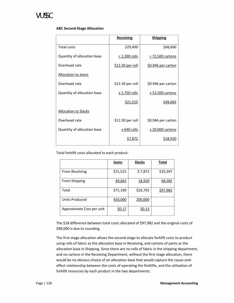
Page | 128 Management Accounting
ABC Second‐Stage Allocation
Receiving Shipping
Total costs
Quantity of allocation base
Overhead rate
Allocation to Jeans
Overhead rate
Quantity of allocation base
Allocation to Slacks
Overhead rate
Quantity of allocation base
$29,400
÷ 2,390 rolls
$12.30 per roll
$12.30 per roll
x 1,750 rolls
$21,525
$12.30 per roll
x 640 rolls
$7,872
$68,600
÷ 72,500 cartons
$0.946 per carton
$0.946 per carton
x 52,500 cartons
$49,665
$0.946 per carton
x 20,000 cartons
$18,920
Total forklift costs allocated to each product:
Jeans Slacks Total
From Receiving $21,525 $ 7,872 $29,397
From Shipping 49,665 18,920 68,585
Total $71,190 $26,792 $97,982
Units Produced 420,000 200,000
Approximate Cost per unit $0.17 $0.13
The $18 difference between total costs allocated of $97,982 and the original costs of
$98,000 is due to rounding.
The first‐stage allocation allows the second‐stage to allocate forklift costs to product
using rolls of fabric as the allocation base in Receiving, and cartons of pants as the
allocation base in Shipping. Since there are no rolls of fabric in the shipping department,
and no cartons in the Receiving Department, without the first stage allocation, there
would be no obvious choice of an allocation base that would capture the cause‐and‐
effect relationship between the costs of operating the forklifts, and the utilization of
forklift resources by each product in the two departments.

Management Accounting Page | 129
Conclusion
The traditional costing method allocates more forklift costs to slacks than to jeans on a
per‐unit basis because casual slacks require more sewing effort. ABC allocates more
forklift costs to jeans than to casual slacks, on a per‐unit basis, which is intuitive
because denim is a heavier‐weight fabric than cotton twill.
STEPS TO IMPLEMENT ACTIVITY‐BASED COSTING
1. Identify and assess ABC needs ‐ Determine viability of ABC method within an
organization.
2. Training requirements ‐ Basic training for all employees and workshop sessions
for senior managers.
3. Define the project scope ‐ Evaluate mission and objectives for the project.
4. Identify activities and drivers ‐ Determine what drives what activity.
5. Create a cost and operational flow diagram – How resources and activities are
related to products and services.
6. Collect data – Collecting data where the diagram shows operational
relationship.
7. Build a software model, validate and reconcile.
8. Interpret results and prepare management reports.
9. Integrate data collection and reporting.
COST HIERARCHY
In ABC, cost pools are often established for each level in a hierarchy of costs. For
manufacturing firms, the following cost hierarchy is commonly identified:
1. Unit‐level costs: For any given product, these costs change in a more‐or‐less
linear fashion with the number of units produced. For example, fabric and
thread are unit‐level costs for an apparel manufacturer: if the company wants
to double production, it will need twice as much fabric and thread.
2. Batch‐level costs: These costs change in a more‐or‐less linear fashion with the
number of batches run. Machine setup costs are often batch‐level costs. The
time required to prepare a machine to run one batch of product is usually
independent of the number of units in the batch: the same time is required to
prepare the machine to run a batch of 100 units as a batch of 50 units. Hence,
batch‐level costs do not necessarily vary in a linear fashion with the number of
units produced.
3. Product‐level costs: These costs are usually fixed and direct with respect to a
given product. An example is the salary of a product manager with
responsibility for only one product. The product manager’s salary is a fixed cost
to the company for a wide range of production volume levels. However, if the
company drops the product entirely, the product manager is no longer needed.
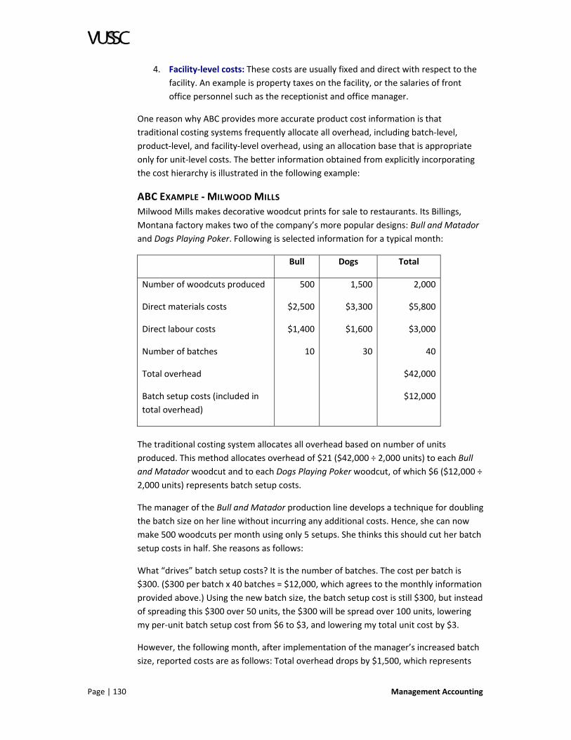
Page | 130 Management Accounting
4. Facility‐level costs: These costs are usually fixed and direct with respect to the
facility. An example is property taxes on the facility, or the salaries of front
office personnel such as the receptionist and office manager.
One reason why ABC provides more accurate product cost information is that
traditional costing systems frequently allocate all overhead, including batch‐level,
product‐level, and facility‐level overhead, using an allocation base that is appropriate
only for unit‐level costs. The better information obtained from explicitly incorporating
the cost hierarchy is illustrated in the following example:
ABC EXAMPLE ‐ MILWOOD MILLS
Milwood Mills makes decorative woodcut prints for sale to restaurants. Its Billings,
Montana factory makes two of the company’s more popular designs: Bull and Matador
and Dogs Playing Poker. Following is selected information for a typical month:
Bull Dogs Total
Number of woodcuts produced
Direct materials costs
Direct labour costs
Number of batches
Total overhead
Batch setup costs (included in
total overhead)
500
$2,500
$1,400
10
1,500
$3,300
$1,600
30
2,000
$5,800
$3,000
40
$42,000
$12,000
The traditional costing system allocates all overhead based on number of units
produced. This method allocates overhead of $21 ($42,000 ÷ 2,000 units) to each Bull
and Matador woodcut and to each Dogs Playing Poker woodcut, of which $6 ($12,000 ÷
2,000 units) represents batch setup costs.
The manager of the Bull and Matador production line develops a technique for doubling
the batch size on her line without incurring any additional costs. Hence, she can now
make 500 woodcuts per month using only 5 setups. She thinks this should cut her batch
setup costs in half. She reasons as follows:
What “drives” batch setup costs? It is the number of batches. The cost per batch is
$300. ($300 per batch x 40 batches = $12,000, which agrees to the monthly information
provided above.) Using the new batch size, the batch setup cost is still $300, but instead
of spreading this $300 over 50 units, the $300 will be spread over 100 units, lowering
my per‐unit batch setup cost from $6 to $3, and lowering my total unit cost by $3.
However, the following month, after implementation of the manager’s increased batch
size, reported costs are as follows: Total overhead drops by $1,500, which represents

Management Accounting Page | 131
the cost savings from eliminating five batch setups for the Bull and Matador production
line. Hence, total overhead drops from $42,000 to $40,500. The traditional costing
system allocates this $40,500 to 2,000 units as $20.25 per unit. This new overhead rate
represents a savings of $0.75 per unit for every woodcut: every Bull and Matador
woodcut, and every Dogs Playing Poker woodcut. The manager of the Bull and Matador
production line is disappointed. Her reported costs did not decrease by as much as she
had anticipated, because most of the benefit from the reduction in batch setups has
been allocated to the Dogs Playing Poker production line.
An ABC system that explicitly recognizes the cost hierarchy would correct this problem.
Under the old production process, ABC would have allocated costs as follows: The cost
pool for batch setup costs was previously $12,000, which would have been allocated to
the two product lines based on the number of batches run by each line:
Overhead rate = total batch setup costs ÷ total number of batches
= $12,000 ÷ 40 batches = $300 per batch
Batch setup costs of $300 per batch
x 10 batches = $3,000 would have been allocated to Bull,
x 30 batches = $9,000 would have been allocated to Dogs.
In a second‐stage allocation, the $3,000 allocated to the Bull and Matador production
line would have been allocated to 500 units for a cost of $6 per woodcut. This allocation
is the same as under the traditional costing system only because the batch size of 50
woodcuts per batch was originally the same on both production lines.
After the batch size is increased for Bull and Matador, production information is as
follows:
Bull Dogs Total
Number of woodcuts produced
Direct materials costs
Direct labour costs
Number of batches
Total overhead
Batch setup costs (included in total
overhead)
500
$2,500
$1,400
5
1,500
$3,300
$1,600
30
2,000
$5,800
$3,000
35
$40,500
$10,500
Now ABC would allocate costs as follows:
In the first stage: $10,500 ÷ 35 batches = $300 per batch (same as before).

Page | 132 Management Accounting
$300 per batch x 5 batches = $1,500 to Bull and Matador (50% less than
before),
$300 per batch x 30 batches = $9,000 to Dogs Playing Poker (same as
before).
In the second stage, the $1,500 is allocated to the 500 Bull and Matador woodcuts, for
$3 per woodcut. This $3 per woodcut reflects the cost savings originally anticipated by
the manager of the Bull and Matador production line. The cost per woodcut for Dogs
Playing Poker remains unchanged ($9,000 ÷ 1,500 units = $6), which is appropriate
because nothing has changed on the Dogs Playing Poker production line.
ABC IN THE SERVICE SECTOR
ABC is as important to companies in the merchandising and service sectors as to
manufacturing companies. In fact, although the origination of ABC is generally ascribed
to manufacturing companies in the 1980s, by then hospitals were already allocating
overhead costs to departments and then to patient services using methods similar to
ABC. Hospitals were required to implement relatively sophisticated allocation processes
in order to comply with Medicare reimbursement rules. After its inception in the 1960s,
Medicare established detailed rules regarding how overhead costs should be grouped
into cost pools, and the choice of appropriate allocation bases for allocating overhead
costs to departments and then to patients. Within these rules, hospitals were able to
maximize revenues by shifting costs from areas such as pediatrics, labour and delivery,
and maternity (which have low rates of Medicare utilization) to the intensive care unit,
the critical care unit, and surgery (which have higher rates of Medicare utilization).
Other non‐manufacturing industries that have benefited from ABC include financial
services firms and retailers.
ABC IMPLEMENTATION ISSUES
Another refinement in product costing that often accompanies implementation of ABC
focuses on step #2 of the five‐step product costing sequence: “identify the direct costs
associated with the cost object.” The refinement involves the following. For a given cost
object, the company attempts to identify costs currently treated as overhead that have
not been—but can be—traced directly to the cost object. In other words, costs are
moved from the overhead cost pool to the direct cost category. For example, an
accounting firm might take certain office‐support expenses formerly treated as
overhead, such as printing and copying, and start tracking and assigning these costs to
specific jobs (audits, tax engagements, etc.) for internal reporting and profitability
analysis (but not necessarily for client billing purposes).
The successful implementation of ABC usually requires participation by managers from
non‐accounting functions, such as production and marketing. Because ABC focuses on
activities, and activities often cut across departments and functional areas,
implementing ABC can improve lines of communication and cooperation within the
company. On the other hand, more accurate cost allocation does not, by itself, reduce
costs. The initial move from a traditional costing system to ABC usually shifts overhead

Management Accounting Page | 133
costs from some products to other products, with some managers “winning” and some
“losing.” Some companies have found that hiring an outside consulting firm to assist
with the ABC adoption facilitates obtaining “buy‐in” by managers and employees
throughout the company. Perhaps partly for this reason, ABC implementation has
become an important consulting product for accounting firms and for many consulting
firms.
Although ABC should provide the company more accurate information, it is not a
panacea; some companies that invested time and money implementing ABC did not
realize the benefits they expected. Some of these companies have reverted to simpler,
more traditional costing systems.
LESSON PROBLEMS
Now review the following problems and answer the related questions. Record your
answers in your course workbook.
Problem 1
Colorado Airlines is operating at capacity on its Denver to New York route, offering
three flights each day on this route, using Boeing 737’s, each with a capacity of 120
passengers. Airline management wants to determine the least expensive way to
increase daily capacity from 360 passengers to 480 passengers. One possibility is to add
one more Boeing 737 per day. The other possibility is to replace the current equipment
with Boeing 727’s, which hold 160 passengers each. In either case, management
believes the planes will continue to operate at capacity.
To ascertain the least expensive way to increase passenger capacity on the Denver‐to‐
New York route, management has asked you to determine what “drives” the airline’s
operating costs.
Consider the following cost drivers:
Number of flights per day.
Number of miles flown per day.
Number of passengers served per day.
Number of passenger miles (miles flown per day multiplied by number of
passengers).
For each of the following costs, identify the most appropriate cost driver from the
above list.
a. Passenger meals.
b. Airplane fuel.
c. Ground personnel who refuel the plane, and mechanics on the ground.
d. Ground personnel who serve passengers at the ticket counter and at the gate.
e. Cockpit crew salaries (Federal Aviation Administration regulations limit pilots to
fly no more than a certain number of hours per month).

Page | 134 Management Accounting
f. Flight attendant salaries (assume that Federal Aviation Administration
regulations limit flight attendants to fly no more than a certain number of hours
per month, and require one flight attendant for every 40 passengers).
g. Economic depreciation of the airplane (i.e., without regard to the depreciation
method chosen for accounting purposes, choose the cost driver that best
captures the wear and tear on the equipment, and determines the economic
life of the plane).
h. Personnel who handle baggage.
Problem 2
You are the Chief Financial Officer of a large New York hospital that has decided to
implement activity‐based costing. Which of the following would you choose as the
allocation base for allocating the costs of the Linen and Laundry Department to the four
patient wards that utilize linen and laundry services, if your objective is to generate the
most accurate cost information possible? The four wards are: (1) surgery, (2) adolescent
care, (3) maternity and nursery, and (4) paediatric care.
a. Patient occupancy rates (i.e., patient days) in each ward.
b. The number of washing machines in the Laundry and Linen Department
c. The number of Medicare patients in each ward.
d. The number of patient admissions to each ward.
Problem 3: In which of the following situations are the techniques of activity‐based
costing most likely to lead to improved production or marketing decisions.
(I) The All‐Direct Company, which incurs significant direct costs, but no overhead costs,
to manufacture its extensive and ever‐changing product line.
(II) The One‐Size‐Fits‐All Hat Company, which makes a single product that is sold to
many different kinds of retailers, in varying volumes, through various marketing
channels, in many different geographic regions.
(III) The Iowa Wind Turbine Electric Cooperative, which has direct costs and fixed
overhead, but no variable overhead.
a. (I) and (II), but not (III)
b. (I) and (III), but not (II)
c. (I) only
d. (II) only
Problem 4
For a generic manufacturing facility (i.e., without being told what the factory makes):
a. Give two examples of overhead expenses for which direct labour hours is a more
appropriate allocation base than machine time.
b. Give two examples of overhead expenses for which machine time is a more
appropriate allocation base than direct labour hours.

Management Accounting Page | 135
Problem 5
The Silver City Mining Company mines copper and aluminium in Southwestern New
Mexico. Traditionally, overhead costs were allocated to the two metals based on direct
labour hours. Using this method in 2005, overhead costs per ton are $50 for aluminium
and $60 for copper.
The company switched to activity‐based costing, using multiple cost pools, and
allocating each cost pool using an allocation base that more accurately captures the
cause and effect relationship between the mining operations and overhead costs. Also,
several overhead cost categories were reclassified as direct costs. The company had
used an Actual Costing system prior to implementing ABC (i.e., overhead rates were
calculated at the end of the year, when actual amounts were known), and continued to
use Actual Costing after implementation of ABC. To study the effect of the new ABC
system, it was retroactively applied to 2005, in order to compare the results to the old
method. Which of the following outcomes under the new system suggests that an error
was made in the calculation of overhead rates?
a. The new overhead rates were $45 per ton of aluminium and $62 per ton of
copper.
b. The new overhead rates were $45 per ton of aluminium and $58 per ton of
copper.
c. The new overhead rates were $55 per ton of aluminium and $58 per ton of
copper.
d. The new overhead rates were $55 per ton of aluminium and $62 per ton of
copper.
Problem 6
The Santa Cruz Candy Company makes five types of candies in its sole factory, including
chocolate truffles and chocolate mints. Truffles are hand‐dipped, so making truffles is
labour‐intensive, and furthermore, only the most experienced (and highest paid)
employees can make truffles. Production of mints is highly automated: they don’t
require much labour, but the machine operators are also highly‐skilled and highly‐paid.
The manager of truffles production (Candy Lowenski) and the manager of mints
production (Coco Hernandez) are discussing their preferences for how factory overhead
should be allocated to their products. The three choices are direct labour dollars, direct
labour hours, and machine hours. Of course, each manager would like to report the
highest profits possible from her product line.
a. In one, two or three (no more than three) complete sentences (each sentence
must have a verb and a period, among other grammatical components), predict
what position each manager will take with respect to her preferred allocation
base, and explain your reasoning.

Page | 136 Management Accounting
Problem 7
The Braintree Furniture Company manufactures two lines of furniture: an upscale,
handcrafted line called Richleau, which is produced in small quantities; and a mass‐
produced, inexpensive line called Particleboard. Both lines are made in the same
factory. Richleau is very labour intensive relative to Particleboard. Braintree just
switched from a traditional costing method that allocated overhead based on direct
labour hours to an activity‐based costing system. Under activity‐based costing, the
amount of overhead allocated to Richleau will be
a. higher than under the traditional costing method.
b. lower than under the traditional costing method.
c. either higher or lower than under the traditional costing method, depending on
the underlying economics of the business.
d. lower than under traditional costing, as long as activity‐based costing is
implemented in a way that provides more accurate cost information.
Problem 8
The not‐for‐profit health clinic Shots‐Я‐Us provides various types of vaccinations and
other shots, especially flu shots, to the public for free or for a nominal fee. The clinic is
funded by several local governmental agencies as well as by a number of charitable
organizations. Since different donors wish to fund different types of shots, the clinic
determines the full cost of each type of shot, by adding overhead to the direct costs,
and then provides this information to current and prospective donors.
Following are actual and budgeted costs for Shots‐Я‐Us for 2003:
Actual Budgeted
Number of patient visits
Number of shots administered
Fixed overhead: salaries, rent for the facility,
insurance, depreciation.
Variable overhead: nursing staff hourly wages,
utilities, disposable supplies.
Cost of hypodermics (a direct cost)
Cost of medications (a direct cost)
5,000
6,000
$94,000
$66,000
$1,000
$30,000
4,000
4,500
$110,000
$40,500
$750
$20,000
Which of the following is probably not a significant cost driver for variable overhead,
and hence, would probably be a poor choice as the cost allocation base for allocating
variable overhead?
a. The number of shots administered

Management Accounting Page | 137
b. The dollar value of the medication administered
c. The number of patient visits
d. The amount of nursing staff time spent administering each type of shot
Problem 9
Pink Ink, Inc. has two products and two overhead cost pools:
Product
A
Product
B
In Total
Units produced
Direct Costs (per unit):
Materials
Labour (paid $20 per hour)
Materials Handling cost pool
Everything Else cost pool
200
$10
$20
50
$20
$40
$24,000
$76,000
a. Using direct labour hours as the allocation base, what is the overhead rate for
Materials Handling overhead?
b. What is the total cost to make each unit of Product B, if all overhead is allocated
based on units produced?
c. How much Everything Else overhead would be applied to each unit of product
A, if this cost pool is allocated to product using direct materials dollars as the
allocation base?
Problem 10
Following is information about Aztech Industries:
Model
A
Model
B
Model
C
Total
Units produced
Direct materials (per unit)
Direct labour (per unit)
Cost driver information:
number of parts (per unit)
direct labour hours (per unit)
300
$50
$20
20
3
500
$75
$50
42
4.60
200
$100
$40
30
4
1,000
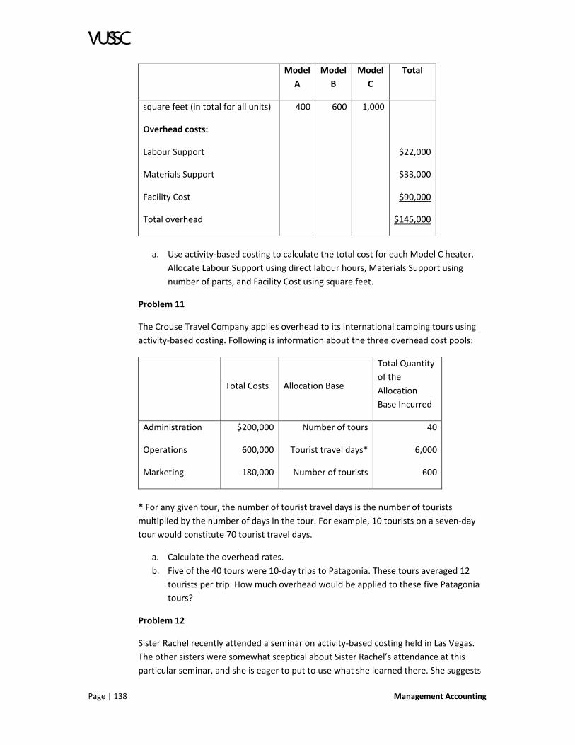
Page | 138 Management Accounting
Model
A
Model
B
Model
C
Total
square feet (in total for all units)
Overhead costs:
Labour Support
Materials Support
Facility Cost
Total overhead
400
600
1,000
$22,000
$33,000
$90,000
$145,000
a. Use activity‐based costing to calculate the total cost for each Model C heater.
Allocate Labour Support using direct labour hours, Materials Support using
number of parts, and Facility Cost using square feet.
Problem 11
The Crouse Travel Company applies overhead to its international camping tours using
activity‐based costing. Following is information about the three overhead cost pools:
Total Costs
Allocation Base
Total Quantity
of the
Allocation
Base Incurred
Administration
Operations
Marketing
$200,000
600,000
180,000
Number of tours
Tourist travel days*
Number of tourists
40
6,000
600
* For any given tour, the number of tourist travel days is the number of tourists
multiplied by the number of days in the tour. For example, 10 tourists on a seven‐day
tour would constitute 70 tourist travel days.
a. Calculate the overhead rates.
b. Five of the 40 tours were 10‐day trips to Patagonia. These tours averaged 12
tourists per trip. How much overhead would be applied to these five Patagonia
tours?
Problem 12
Sister Rachel recently attended a seminar on activity‐based costing held in Las Vegas.
The other sisters were somewhat sceptical about Sister Rachel’s attendance at this
particular seminar, and she is eager to put to use what she learned there. She suggests

Management Accounting Page | 139
that the orphanage implement a refined costing system, and she develops the following
information.
Costs vary with the age of the children. The number and ages of children were as
follows:
2000 2001
Pre‐school
(ages 0 ‐ 5)
30 15
Pre‐teen
(ages 6 – 12)
30 32
Teenagers
(ages 13 ‐ 18)
Total
20
80
25
72
Everyone agrees that 2000 was a very successful year for the Orphanage, so the 2001
budget was based on 2000 actual costs. The following information pertains to 2000:
Food costs per meal were $4 for pre‐schoolers, $5 for pre‐teens, and $6.50 for
teenagers. 3 meals are served per day, 365 days per year.
The cost of clothing is twice as much (per child) for teenagers as for the other
two age groups.
Laundry and linen costs per child do not vary with the age of the child.
However, this category also includes the cost of a diaper service. 1/3 of pre‐
school children are in diapers, and the cost is $15 per week, 52 weeks per year.
Educational costs do not apply to pre‐school children.
Only teenagers receive an allowance. The allowance is $20 per week, 50 weeks
per year.
a. Identify the cost drivers for the following expenses:
Diaper service.
Educational costs.
Allowances .
b. Prepare a flexible budget for 2001, making use of the information compiled by
Sister Rachel, as well as information about fixed costs from the original 2001
budget.
c. Should Sister Sarah be satisfied with the orphanage’s financial results and
efforts to control costs in 2001? Briefly explain.

Page | 140 Management Accounting
Problem 13
The 601 Blue Jean Company has decided to allocate the cost of its Warehouse and
Distribution Centre to its customers using activity‐based costing, in order to better
assess profitability by customer. The warehouse manager determines that the only
costs that are economically feasible to trace directly to the customer are outbound
freight costs. The manager then decides that the following overhead cost pools should
be allocated to customers using the following cost drivers:
Overhead Cost Pool Cost Driver (Allocation Base)
Order Processing Department
Order Filling Department
Quality Control Department
Shipping Department
Number of individual orders processed for that customer
Number of line items on all pull‐tickets for that customer
Number of cartons shipped to that customer
Number of cartons shipped to that customer
Following are relevant data for each overhead cost pool:
Order Processing Department
Total costs for this department
Total number of orders processed
Order Filling Department
Total costs for this department
Total number of line‐items on all pull tickets
Quality Control Department
Total costs for this department
Total number of cartons shipped
Shipping Department
Total costs for this department
Total number of cartons shipped
$3,000,000
200,000
$4,000,000
4,000,000
$500,000
2,000,000
$7,500,000
2,000,000
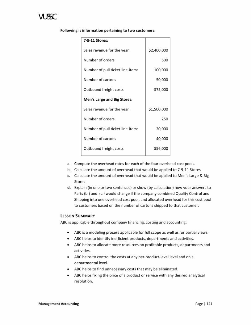
Management Accounting Page | 141
Following is information pertaining to two customers:
7‐9‐11 Stores:
Sales revenue for the year
Number of orders
Number of pull ticket line‐items
Number of cartons
Outbound freight costs
Men’s Large and Big Stores:
Sales revenue for the year
Number of orders
Number of pull ticket line‐items
Number of cartons
Outbound freight costs
$2,400,000
500
100,000
50,000
$75,000
$1,500,000
250
20,000
40,000
$56,000
a. Compute the overhead rates for each of the four overhead cost pools.
b. Calculate the amount of overhead that would be applied to 7‐9‐11 Stores
c. Calculate the amount of overhead that would be applied to Men’s Large & Big
Stores
d. Explain (in one or two sentences) or show (by calculation) how your answers to
Parts (b.) and (c.) would change if the company combined Quality Control and
Shipping into one overhead cost pool, and allocated overhead for this cost pool
to customers based on the number of cartons shipped to that customer.
LESSON SUMMARY
ABC is applicable throughout company financing, costing and accounting:
ABC is a modeling process applicable for full scope as well as for partial views.
ABC helps to identify inefficient products, departments and activities.
ABC helps to allocate more resources on profitable products, departments and
activities.
ABC helps to control the costs at any per‐product‐level level and on a
departmental level.
ABC helps to find unnecessary costs that may be eliminated.
ABC helps fixing the price of a product or service with any desired analytical
resolution.

Page | 142 Management Accounting
LESSON 3.5: ALLOCATION OF SERVICE DEPARTMENT COSTS
LESSON INTRODUCTION
As organizations grow they may create departments that do not directly service
customers, but support the production process or other activities important to
company operations. One example would be an IT department that supports the
operation of servers and computer technologies within the company. In this case the
cost of operating the IT department is deemed to an expense and the cost of these
services are shared among departments.
Service department costs are factory overhead costs. Since the production
departments are directly benefitted by service departments, the costs of a service
department should be allocated to the appropriate production departments (as part of
factory overhead costs). In this lesson we will explore how to do this.
LESSON OBJECTIVES
Upon completion of this lesson you will be able to:
1. Employ the following methods for calculating service department costs:
a. The Direct Method
b. The Step‐Down Method
c. The Reciprocal Method
2. Identify functional incentives from service department cost allocations.
INTRODUCTION TO SERVICE DEPARTMENT COSTING
Many companies in all sectors of the economy, and not‐for‐profit and governmental
organizations as well, allocate service department costs to “production” or user
departments, and ultimately to the products and services that they provide. For
example, hospitals use sophisticated methods for allocating costs of service
departments such as Housekeeping, Patient Admissions, and Medical Records to patient
wards and outpatient services, and then to individual patients. Historically, these
allocations were important to hospitals because Medicare reimbursement was based on
actual costs. To the extent that the hospital allocated service department costs to
Medicare patients, Medicare covered these costs.
Companies that allocate service department costs do so for one or more of the
following reasons:
1. To provide more accurate product cost information. Allocating service
department costs to production departments, and then to products, recognizes
that these services constitute an input in the production process.
2. To improve decisions about resource utilization. By imposing on division
managers the cost of the service department resources that they use, division
managers are encouraged to use these resources only to the extent that their
benefit exceeds their cost.
3. To ration limited resources. When production departments have some
discretion over their utilization of a service department resource, charging

Management Accounting Page | 143
production departments for the resource usually results in less demand for it
than if the resource were “free” to the production departments.
The motivation for the first reason, to provide more accurate product cost information,
can be to improve decision‐making within the organization, to improve the quality of
external financial reporting, or to comply with contractual agreements in regulatory
settings where cost‐based pricing is used. As discussed above, Medicare was historically
a cost‐based reimbursement scheme. As another example, defence contractors that
provide the U.S. military “big ticket” items such as airplanes and ships often operate
under cost‐plus contracts, under which they are reimbursed for their production costs
plus a guaranteed profit. In such settings, the calculation of cost includes a reasonable
allocation of overhead, including overhead from service departments.
The distinction between the second and third reasons is important in the context of
fixed versus variable costs. In connection with the second reason, to improve decisions
about resource utilization, from the company’s perspective, a division manager making
a short‐term decision about whether to utilize service department resources should
incorporate into that decision the service department’s marginal costs, which are
usually the variable costs. The manager should ignore the service department’s fixed
costs if these costs will not be affected by the manager’s decision. This reasoning
suggests that only the service department’s variable costs should be charged out.
However, in connection with the third reason, to ration a scarce resource, if the service
department controls a fixed asset, and if demand for the asset exceeds capacity,
charging users a fee for the asset allows the service department to balance demand
with supply. The fee need not relate to the cost of obtaining the asset; rather, it is a
mechanism for managing demand. Examples would be charging departments a “rental
fee” for their use of vehicles from the motor pool, or for their use of a corporate
conference facility.
Service department costs can be allocated based on actual rates or budgeted rates.
Actual rates ensure that all service department costs are allocated. Budgeted rates
provide service department managers incentives to control costs, and also provide user
departments more accurate information about service department billing rates for
planning purposes. In either case, service department costs should be allocated using an
allocation base that reflects a cause‐and‐effect relationship, whenever possible. Here
are some examples:
Allocate building maintenance costs based on square footage;
Allocate costs of the company airplane based on miles flown; and
Allocate costs of the data processing department based on CPU time.
In some cases, companies benefit from allocating fixed costs using a different allocation
base than variable costs. For example, fixed costs might be allocated based on an
estimate of long‐term usage by the production departments.

Page | 144 Management Accounting
Historically, there have been three alternative methods for allocating service
department costs. These methods differ in the extent to which they recognize that
service departments provide services to other service departments as well as to
production departments. All three methods ultimately allocate all service department
costs to production departments; no costs remain in the service departments under any
of the three methods.
THE DIRECT METHOD
The direct method is the most widely‐used method. This method allocates each service
department’s total costs directly to the production departments, and ignores the fact
that service departments may also provide services to other service departments.
Example: Human Resources (H.R.), Data Processing (D.P.), and Risk Management (R.M.)
provide services to the Machining and Assembly production departments, and in some
cases, the service departments also provide services to each other, as reflected in the
following table:
Total Cost Service
Dept..
% of services provided by the service department listed
at left to:
H.R. D.P. R.M. Machining Assembly
$ 80,000 H.R. ‐‐ 20% 10% 40% 30%
120,000 D.P. 8% ‐‐ 7% 30% 55%
40,000 R.M. ‐‐ ‐‐ ‐‐ 50% 50%
$240,000
The amounts in the far left column are the costs incurred by each service department.
The percentages in the other columns are the percentage of each service department’s
services provided to each department that utilizes the services of that service
department. These percentages are derived from some relevant measure of service
department activity. For example, the percentages for human resources might be based
on the number of employees in each department, or the number of new hires in each
department. The percentages for data processing might be based on the number of
computers in each department. Any services that a department provides to itself are
ignored, so the intersection of the row and column for each service department shows
zero. The rows sum to 100%, so that all services provided by each service department to
the other departments are accounted for.
Under the direct method, each service department is allocated separately, and the
order in which the service departments are allocated does not matter. Taking one row
at a time, the percentages of the production departments are normalized, so that they
add up to 100% while still reflecting the relative usage by the production departments
(relative to all of the other production departments). For example, in applying the direct

Management Accounting Page | 145
method for the costs of human resources, Machining and Assembly are the only
production departments that used the services of the Human Resources Department in
March, so the percentages in the columns for machining and assembly are the only
percentages that are relevant (the 20% for data processing and the 10% for risk
management are ignored). The denominator in the normalization process is the sum of
the percentages of all of the production departments. For example, for the human
resources row in the table below, the 70% is the sum of 40% for machining and 30% for
assembly in the table above.
Total
Cost
Service
Dept..
Normalized percentage of services provided by the service
department listed at left to the production departments:
H.R. D.P. R.M. Machining Assembly
$ 80,000 H.R. ‐‐ ‐‐ ‐‐ 40% ÷ 70% = 57% 30% ÷ 70% = 43%
120,000 D.P. ‐‐ ‐‐ ‐‐ 30% ÷ 85% = 35% 55% ÷ 85% = 65%
40,000 R.M. ‐‐ ‐‐ ‐‐ 50% 50%
$240,000
The risk management service department percentages do not require normalization,
because this service department provided services only to the production departments,
it did not provide any services to the other service departments. The normalized per‐
centages are then used to allocate each service department’s total costs to the produc‐
tion departments:
Total cost Service
Dept..
Machining Assembly
$ 80,000 H.R. 57% x $80,000 = $45,600 43% x $80,000 = $34,400
120,000 D.P. 35% x $120,000 = $42,000 65% x $120,000 = $78,000
40,000 R.M. 50% x $40,000 = $20,000 50% x $40,000 = $20,000
$240,000 $107,600 $132,400
The normalization process ensures that the sum of the costs allocated to the production
departments equals the total costs incurred by each service department, even though
service‐department‐to‐service‐department services are ignored. For example, $42,000
of data processing costs are allocated to machining and $78,000 are allocated to
assembly, and these two amounts sum to $120,000, the total costs incurred by data
processing.

Page | 146 Management Accounting
THE STEP‐DOWN METHOD
The step‐down method is also called the sequential method. This method allocates the
costs of some service departments to other service departments, but once a service
department’s costs have been allocated, no subsequent costs are allocated back to it.
The choice of which department to start with is important. The sequence in which the
service departments are allocated usually effects the ultimate allocation of costs to the
production departments, in that some production departments gain and some lose
when the sequence is changed. Hence, production department managers usually have
preferences over the sequence. The most defensible sequence is to start with the
service department that provides the highest percentage of its total services to other
service departments, or the service department that provides services to the most
number of service departments, or the service department with the highest costs, or
some similar criterion.
Example: Human Resources (H.R.), Data Processing (D.P.), and Risk Management (R.M.)
provide services to the Machining and Assembly production departments, and in some
cases, the service departments also provide services to each other:
Total Cost
Service
Dept.
% of services provided by the service
department listed at left to:
H.R. D.P. R.M. Machining Assembly
$ 80,000 H.R. ‐‐ 20% 10% 40% 30%
120,000 D.P. 8% ‐‐ 7% 30% 55%
40,000 R.M. ‐‐ ‐‐ ‐‐ 50% 50%
$240,000
The amounts in the far left column are the costs incurred by each service department.
Any services that a department provides to itself are ignored, so the intersection of the
row and column for each service department shows zero. The rows sum to 100%, so
that all services provided by each service department are charged out.
The company decides to allocate the costs of Human Resources first, because it
provides services to two other service departments, and provides a greater percentage
of its services to other service departments. However, a case could be made to allocate
Data Processing first, because it has greater total costs than either of the other two
service departments. In any case, the company decides to allocate Data Processing
second.
In the table below, the row for each service department allocates the total costs in that
department (the original costs incurred by the department plus any costs allocated to it
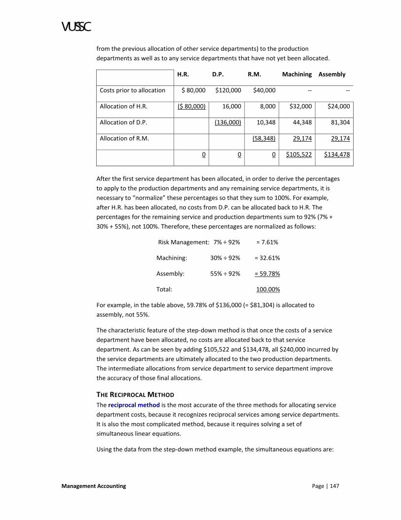
Management Accounting Page | 147
from the previous allocation of other service departments) to the production
departments as well as to any service departments that have not yet been allocated.
H.R. D.P. R.M. Machining Assembly
Costs prior to allocation $ 80,000 $120,000 $40,000 ‐‐ ‐‐
Allocation of H.R. ($ 80,000) 16,000 8,000 $32,000 $24,000
Allocation of D.P. (136,000) 10,348 44,348 81,304
Allocation of R.M. (58,348) 29,174 29,174
0 0 0 $105,522 $134,478
After the first service department has been allocated, in order to derive the percentages
to apply to the production departments and any remaining service departments, it is
necessary to “normalize” these percentages so that they sum to 100%. For example,
after H.R. has been allocated, no costs from D.P. can be allocated back to H.R. The
percentages for the remaining service and production departments sum to 92% (7% +
30% + 55%), not 100%. Therefore, these percentages are normalized as follows:
Risk Management: 7% ÷ 92% = 7.61%
Machining: 30% ÷ 92% = 32.61%
Assembly: 55% ÷ 92% = 59.78%
Total: 100.00%
For example, in the table above, 59.78% of $136,000 (= $81,304) is allocated to
assembly, not 55%.
The characteristic feature of the step‐down method is that once the costs of a service
department have been allocated, no costs are allocated back to that service
department. As can be seen by adding $105,522 and $134,478, all $240,000 incurred by
the service departments are ultimately allocated to the two production departments.
The intermediate allocations from service department to service department improve
the accuracy of those final allocations.
THE RECIPROCAL METHOD
The reciprocal method is the most accurate of the three methods for allocating service
department costs, because it recognizes reciprocal services among service departments.
It is also the most complicated method, because it requires solving a set of
simultaneous linear equations.
Using the data from the step‐down method example, the simultaneous equations are:

Page | 148 Management Accounting
H.R. = $ 80,000 + (0.08 x D.P.)
D.P. = $120,000 + (0.20 x H.R.)
R.M. = $ 40,000 + (0.10 x H.R.) + (0.07 x D.P.)
Where the variables H.R., D.P. and R.M. represent the total costs to allocate from each
of these service departments. For example, Human Resources receives services from
Data Processing, but not from Risk Management. 8% of the services that Data
Processing provides, it provides to Human Resources. Therefore, the total costs
allocated from Human Resources should include not only the $80,000 incurred in that
department, but also 8% of the costs incurred by Data Processing. Solving for the three
unknowns (which can be performed using spreadsheet software):
H.R. = $ 91,057
D.P. = $138,211
R.M. = $ 58,781
Hence, costs are allocated as follows:
H.R. D.P. R.M. Machining Assembly
Costs prior to
allocation
$80,000 $120,000 $40,000 ‐‐ ‐‐
Allocation of H.R. ($91,057) 18,211 9,106 $36,423 $ 27,317
Allocation of D.P. 11,057 (138,211) 9,675 41,463 76,016
Allocation of R.M. (58,781) 29,390 29,390
$ 0 $ 0 $ 0 $107,276 $132,723
To illustrate the derivation of the amounts in this table, the $36,423 that is allocated
from Human Resources to Machining is 40% of H.R.’s total cost of $91,057.
SUMMARY OF SERVICE DEPARTMENT COST ALLOCATION METHODS
The direct method and step‐down method have no advantages over the reciprocal
method except for their simplicity, and the step‐down method is sometimes not very
simple. Nevertheless, the reciprocal method is not widely used. Given advances in
computing power, the reciprocal method would seem to be accessible to many
companies that are not using it. Presumably, these companies believe that the benefits
obtained from more accurate service department cost allocations do not justify the
costs required to implement the reciprocal method. In fact, many companies do not
allocate service department costs at all, either because they do not think these
allocations are beneficial, or because they do not believe that the benefits justify the
costs.

Management Accounting Page | 149
DYSFUNCTIONAL INCENTIVES FROM SERVICE DEPARTMENT COST ALLOCATIONS
The incentives that service department cost allocations impose on managers and
employees should be carefully considered. In some cases, these allocations have
unintended and undesirable consequences. For example:
At one university, professors are “charged” for office telephone usage, which includes a
fixed monthly fee similar to the flat fee that is charged for residential telephone service.
The “charge” comes out of the professor’s “research allowance,” which can otherwise
be used for professional expenses such as journal subscriptions, professional
organization dues, and travel to conferences. Since the flat fee (as opposed to the long
distance charges) is unavoidable, it does not affect the professors’ behaviour, but it is
viewed negatively, because the research allowance is effectively several hundred dollars
a year less than “advertised” by the administration.
At another university, state‐of‐the‐art computer equipment in the classrooms is
purchased out of student fees. Consequently, this equipment is readily available and
“free” to the faculty when they teach. However, when a professor reserves a room for a
non‐teaching purpose, such as a research presentation to fellow faculty, the
Instructional Technology service centre “charges” the professor’s department
approximately $50 to use the equipment, which is far in excess of the equipment’s
marginal cost (the depreciation on the bulb in the projector). The $50 charge is
sufficient to dissuade many departments from using the equipment for non‐
instructional purposes, so the equipment sits idle, and the professors use a “low tech”
solution: an overhead projector and transparencies.
LESSON PROBLEMS
Now review the following problems and answer the related questions. Record your
answers in your course workbook.
Problem 1
The Bola Tie Company has two service departments (Departments A and B) and three
production departments (Departments X, Y and Z). Service Department A provides
services to all three production departments as well as to Service Department B.
However, Service Department B only provides services to the other service department
(Department A). In other words, Service Department B provides no services directly to
the production departments. Which of the following methods for allocating service
department costs makes the most sense in this situation?
a. The direct method.
b. The step‐down method, beginning with Service Department A.
c. The step‐down method, beginning with Service Department B.
d. We would want to know the costs incurred by each service department before
determining which allocation method makes the most sense.

Page | 150 Management Accounting
Problem 2
The “Big One” accounting firm has three divisions: audit, tax and consulting; two
support departments: administration and human resources. The following table shows
the utilization of support department services by the user departments:
Admin.
Human
Resources Audit Tax Consulting
Administration 10% 30% 25% 35%
Human Resources 10% 30% 35% 25%
Which of the following allocation methods will result in the smallest allocation of
support department costs to the Consulting Division?
a. The direct method.
b. The step‐down method, beginning with Administration.
c. The step‐down method, beginning with Human Resources.
d. Cannot be determined from the information given.
Problem 3
One advantage of the step‐down method of allocating service department costs to
production departments, over the direct method, is the following:
a. Some interaction among service departments (i.e., service departments
providing services to other service departments) is accounted for.
b. The step‐down method is easier to apply (i.e., it is less complicated).
c. All service department costs are eventually allocated to production
departments.
d. All interaction among service departments (i.e., service departments providing
services to other service departments) is accounted for.
Problem 4
The MIS department of Coldwater Industries provides services to two other service
departments (Accounting and Personnel) and two factories. The cost of operating the
MIS department is $100,000 annually. The volume of services provided to Accounting,
Personnel, and the factories is measured by the number of computer terminals in each
area.
Factory
X
Factory
Y
Accounting Personnel
Number of
terminals
30 10 40 20

Management Accounting Page | 151
a. Using the direct method of service department allocation, calculate the
allocation of MIS costs to Factory X.
Problem 5
Amber Industries has two service departments: Human Resources (H.R.) and
Accounting. These two service departments provide services to each other, and to three
factories, as shown in the following table:
Service
Dept..
Dept..
Operating
Costs
Percentage of services provided by the service department
indicated in the far left column to each of the factories and
service departments
H.R. Accounting Factory A Factory B Factory C
H.R. $350,000 15% 35% 40% 10%
Accounting $880,000 25% 25% 15% 35%
a. Calculate the amount of service department costs that will be allocated to each
of the factories, using the Direct Method of service department cost allocation.
Problem 6
Global‐Mega‐Corp allocates the costs of three service departments to its three
production departments. The following table shows the percentage of services that
each service department provides to each production department and to the other two
service departments:
Human Resources
Data Processing
Legal Dept. Production Dept. 1
Production Dept. 2
Production Dept. 3
Human Resources
15% 15% 35% 15% 20%
Data Processing
15% 10% 25% 30% 20%
Legal Department
15% 25% 25% 20% 15%
The following table shows the costs incurred by each service department, prior to the
allocation of any service department costs to the other service departments:
Human Resources
Data Processing
Legal Department
$101,000
$324,000
$253,000

Page | 152 Management Accounting
a. Using the Direct Method of service department cost allocation, calculate the
total service department costs that are allocated to each production
department.
Problem 7
Xancar Corporation has three factories, and allocates the costs of two service
departments to these factories using the Direct Method of service department cost
allocation. The table below shows the costs incurred by these two service departments
for the most recent year, the allocation base used to allocate the costs of each
department, and the amount of the allocation base incurred by the factories and service
departments.
Costs incurred
Allocation base
Accounting &
Computing
HR Factory in
Zancobar
Factory in Yebasta
Factory in
Quinzotet
Accounting &
Computing
$850,000 Operating
costs
$850,000 $930,000 $1,200,000 $1,100,000 $1,700,000
Human
Resources
$930,000 Number of
employees
45 33 110 75 145
a. Calculate service department costs allocated to each factory.
Problem 8
A company has three service departments that provide services to each other and to
four production departments. Details for 2005 are shown below:
Human
Resources
Accounting Data
Processing
Costs incurred to run the department: $700,000 $1,200,000 $1,400,000
Allocation base used to allocate costs of
the service department to the four
production departments:
FTE’s (full‐
time
employee
equivalents)
Invoices
processed
# of
computers
Amount of services provided by the
service department to itself and to each
of the recipient departments, as
measured by the quantity of the
allocation base incurred in each
department:
Human Resources 9 467 13

Management Accounting Page | 153
Human
Resources
Accounting Data
Processing
Accounting 23 117 25
Data Processing 32 83 40
Production Department A 101 223 32
Production Department B 157 319 44
Production Department C 33 444 37
Production Department D 69 190 17
Total quantity of the allocation base 424 1,843 208
a. Using the Direct Method of service department cost allocation, what are the
total service department costs from the three service departments that will be
allocated to production department B?
Problem 9
The Franklin Corporation allocates the costs of three service departments to its three
production departments. The following table shows the percentage of services that
each service department provides to each production department and to the other two
service departments:
Service
Dept. A
Service
Dept. B
Service
Dept. C
Production
Dept. 1
Production
Dept. 2
Production
Dept. 3
Service Dept. A 20% 20% 30% 10% 20%
Service Dept. B 15% 10% 25% 30% 20%
Service Dept. C 15% 25% 30% 20% 10%
The following table shows the costs incurred by each service department, prior to the
allocation of any service department costs to the other service departments:
Service Dept. A
Service Dept. B
Service Dept. C
$ 80,000
$124,000
$153,000

Page | 154 Management Accounting
a. Using the Direct Method of service department cost allocation, calculate the
total service department costs that are allocated to each production
department.
b. Use the Step‐Down Method of service department cost allocation, and calculate
the total service department costs allocated to Production Department 1.
Assume that Service Department A is allocated first, then Service Department C,
and finally Service Department B.
Problem 10
State Farmers Insurance Company has three revenue‐generating divisions: Property
Insurance, Life Insurance, and Automobile Insurance. The Legal Department is a service
department that provides services to these three revenue‐generating divisions, and not
to any other department. To allocate legal department costs to the user departments,
the lawyers in the Legal Department track the hours they spend providing services to
each department. (These hours are called “lawyer‐billed” hours.) Relevant information
about lawyer‐billed hours is as follows:
Peak
Demand
Average
Demand
Actual
May
Usage
Property Insurance Division
Life Insurance Division
Automobile Insurance
Division
600 hours
200 hours
200 hours
300 hours
180 hours
180 hours
420 hours
170 hours
180 hours
The Legal Department budgets fixed costs at $100,000 monthly, and variable costs at
$16 per lawyer‐billed hour. During May, actual costs incurred were as follows: $70,000
in fixed costs, and $7,000 in variable costs.
a. What is the actual cost per lawyer‐billed hour, using actual costs (fixed and
variable) and the actual level of activity for the month?
b. Allocate May legal costs to the Auto Division, using the rate calculated in Part
(A), based on actual usage.
c. What amount of legal costs for May will be allocated to the Life Division if a dual
allocation rate is used, in which budgeted fixed costs are allocated based on
peak usage requirements, and budgeted variable costs are allocated based on
actual usage?
LESSON SUMMARY
As noted in this lesson there are three basic methods to allocate service department
costs to production departments or customer service organizations: (1) the direct
method; (2) the step down method; and (3) the reciprocal method. The basis for
allocation of service area costs should ideally be causally related to the demands made

Management Accounting Page | 155
on that department by other departments. Both cause‐and‐effect and benefits‐
received criteria are taken into account. If the service departments provide service to
each other (referred to as reciprocal services), the reciprocal method is the most
accurate, the step method next, and final the direct method is the least accurate. With
different service and production departments as cost objects, costs are initially
accumulated on a department‐by‐department basis. Departments working directly on
programs or units of product or service are production departments. The other
departments are service departments. The allocation problem then is to reassign
service department costs to production departments or programs for both performance
evaluation and product or program costing. Within a production department, these
allocated service costs are then reallocated to units of service or product according to
the bases of allocation that each respective production department uses for its indirect
costs.

Page | 156 Management Accounting
LESSON 3.6: THE ROLE OF COST IN SETTING PRICES
LESSON INTRODUCTION
This lesson discusses the role that product costs play in setting sales prices. For most
companies operating in competitive markets, as well as for unregulated monopolies
(such as a pharmaceutical company that has a drug under patent with no close
substitutes), the most important factor in setting the profit‐maximizing sales price is the
elasticity of demand (the sales demand as a function of price). The elasticity of demand
is affected by such factors as competitors’ prices, consumers’ preferences, and the
availability of substitute goods. Ignoring the elasticity of demand, and setting the sales
price based on cost of production (such as full cost plus 30%) is generally a really bad
idea.
Nevertheless, production costs do play a supporting role in setting prices generally, and
for a relatively small number of products and markets, production costs play the lead
role. Let’s explore the concepts related to price setting.
LESSON OBJECTIVES
Upon completion of this lesson you will be able to:
1. Explain the difference between short‐term, intermediate and long‐run pricing
decisions.
2. Select the most appropriate pricing decisions.
3. Explain the impact of regulated monopolies on pricing.
4. Describe cost‐plus contracts.
5. Manage disputes arising from cost‐plus contracts and over pricing.
6. Describe the downward demand spiral.
SHORT‐RUN PRICING DECISIONS
Occasionally, a company faces a sales opportunity for which the only relevant costs and
revenues are the incremental costs and revenues for that one transaction. In this
situation, accurate information about marginal costs are important, because the
company should be willing to set the sales price at any amount in excess of marginal
cost (marginal production cost plus any marginal non‐manufacturing costs such as
distribution and marketing costs). Typically, marginal production costs consist of all
variable production costs.
These opportunities probably occur relatively infrequently (certainly less often, for
example, than one might infer from Eliyahu Goldratt’s popular business novel The Goal).
Among the conditions that are typically required for the optimal sales price to depend
only on the variable costs of the one transaction the company now faces are: (1) excess
production capacity (so that the sales order does not displace existing orders); (2) a
one‐time customer (since the price the customer is willing to pay in the future might
depend on the price the customer pays today); and (3) a customer not in the company’s
normal sales channels (because if other customers learn that the company has given
another customer a price break, they are likely to demand similar concessions).

Management Accounting Page | 157
INTERMEDIATE‐RUN PRICING DECISIONS
Over the course of several months to a year or two, costs associated with many fixed
assets are unavoidable, but the company can make meaningful decisions about product
prices, production levels and product mix. For these decisions, microeconomics
provides analytical tools for jointly determining the optimal sales price and production
level to maximize profits. The solution to this problem depends on the elasticity of
demand and also on variable production costs (marginal production cost, in the
terminology of economics).
LONG‐RUN PRICING DECISIONS
In the long‐run, all fixed costs become relevant costs. Factories and warehouses can be
built, rebuilt, purchased or sold. Salaried employees can be hired, fired, reassigned, or
given incentives to resign or retire. Long‐term leases and other contracts come up for
renewal. In the long‐run, the company’s revenues must exceed its costs, if it is to
survive. Therefore, the management accounting system should provide managers
information about whether sales prices for products are sufficiently in excess of their
full cost of production to cover non‐manufacturing costs and still provide the company
a reasonable rate of return. Management should consider dropping products that are
unable to cover their full costs (manufacturing costs plus non‐manufacturing costs),
unless there are extenuating circumstances such as a product that serves as a “loss
leader” (e.g., sell the inkjet printer at or near cost, and make high profit margins on
sales of ink cartridges). The timing for eliminating unprofitable products might depend
on when the costs of fixed assets associated with those products can be avoided.
PRICING DECISIONS WHEN THE DEMAND FUNCTION IS UNKNOWN
For new products, the demand function is often unpredictable. Also, important macro‐
economic, political and technological changes can create significant uncertainty about
the demand function. In these situations, the sales price might be based on cost of
production. As better information about the demand function becomes known over
time, this information should then be incorporated into pricing decisions.
REGULATED MONOPOLIES
Natural monopolies that provide essential services are usually regulated. Traditionally,
utility companies that provide electricity, natural gas and telephone service have been
natural monopolies in their local service areas. When these services are provided by a
for‐profit company, as opposed to a municipality or cooperative, a regulatory agency
determines the rates that the company is allowed to charge customers, in order to
cover its costs and earn a reasonable return on its investment. Hence, rate‐setting
requires the determination of the utility company’s cost of providing the service. In
effect, sales prices for the utility company are based on its costs.
In the telecommunications industry, changes in technology have created competition
that did not exist before. For example, one can easily purchase cellular phone service
from one of a number of providers, and entirely avoid the company that provides local
land‐line telephone service. Changes in laws and technology permit customers to
purchase long distance telephone service from any of a number of providers. Attempts
Page | 158 Management Accounting
have been made to deregulate the electric and natural gas markets, although the
results have been mixed with respect to consumer welfare. When an industry that was
previously a natural monopoly becomes a competitive market, regulatory rate‐setting is
no longer necessary.
COST‐PLUS CONTRACTS
In a few specialized markets, sales prices are often based on cost. The U.S. Defence
Department frequently contracts with companies for the design and manufacture of
military equipment using cost‐plus contracts: the contractor receives reimbursement
for production costs plus a negotiated profit. Cost‐plus contracts are useful when it is
difficult for the manufacturer to predict production costs, when product specifications
may have to change after the contract is signed, or when there is only one logical
supplier. Military equipment with long design and production lead‐times, such as
complex weapons systems and aircraft, often meet one or more of these criteria.
An important purpose of cost‐plus contracts is to transfer risk from the seller to the
buyer. For example, given the uncertainty surrounding the cost of building the next‐
generation Navy submarine, it is possible that no company capable of undertaking the
project would be willing to do so, if the company were required to commit to a price
beforehand. A significant cost overrun could bankrupt the company. Conversely, if the
contracted price significantly exceeded actual cost, the large profits that would be
earned by the defence contractor could cause the military considerable political
embarrassment. Cost‐plus contracts avoid both issues by ensuring that the defence
contractor earns a reasonable profit.
Medicare, which was discussed earlier, is another government program that originally
used a cost‐plus reimbursement scheme. Another example is Federal support of
scientific research. National Science Foundation grants usually allow grant money to be
used to cover the direct costs of the research as well as a share of institutional
overhead. The indirect cost reimbursement rate is based on estimates of the indirect
costs of the grant recipient. In other words, the indirect cost reimbursement rate is
institution‐specific. When the researcher is employed by a university, which is often the
case, these indirect costs can include general and administrative expenses that
sometimes appear far removed from the researcher and department that receives the
grant.
In the entertainment industry, actors and writers sometimes sign contracts that provide
them a percentage of the profits from a movie or television show. These contracts are
not cost‐plus contracts, but they do incorporate cost in the determination of the
amount to be received by the actor or writer. Risk sharing in this situation does not
apply so much to uncertainty about the cost of production, as to uncertainty about
revenue. These contracts allow the actor or writer to share in the upside potential of
the project.
Management Accounting Page | 159
DISPUTES UNDER COST‐PLUS CONTRACTS
There are fairly complex guidelines for how government contractors can allocate
overhead. These rules have been promulgated by the Cost Accounting Standards Board.
Within these guidelines, contractors that are working on a mix of cost‐plus contracts
and traditional fixed fee contracts have incentives to allocate as much overhead as
possible to the cost‐plus contracts and away from fixed fee contracts. The fixed fee
contracts could represent sales to government agencies or to commercial enterprises.
To the extent that overhead is allocated to the cost‐plus contracts, the contractor will
be reimbursed for those overhead costs. Headlines sometimes report apparently
excessive charges under cost‐plus contracts, such as $500 toilet seats for military
airplanes. Usually, these amounts reflect the allocation of large amounts of overhead,
including research and design, to a relatively small production run and they are not
improper.
On the other hand, contractors also have incentives to shift direct costs from fixed fee
contracts to cost‐plus contracts, and this type of cost‐shifting constitutes fraud. Several
cases have arisen over the past few decades in which defence contractors have been
accused of this practice, as well as other practices involving the improper treatment of
overhead.
In the 1990s, Stanford University came under public scrutiny for allegedly including in its
indirect cost pool, for the purpose of determining reimbursement rates on Federal
grants, the cost of depreciation on a yacht that had been donated to the University, and
the cost of expensive linen at the University President’s house. The inclusion of these
costs was apparently not a concerted effort to increase the reimbursement rate. In
point of fact, however, Stanford had one of the highest reimbursement rates of any
university in the nation, and Stanford put on seminars, attended by personnel from
other universities, on how to maximize reimbursement under Federal grants. At one
point, University President Donald Kennedy remarked “I expect our controllers to do
their best on behalf of the university.” There were Congressional hearings, and the
scandal prompted Kennedy to resign.
There have been so many public allegations over the years by actors and writers that
film and television studios overstate costs, and thus significantly reduce or completely
eliminate the incentive component of the actor’s or writer’s contract, that it is difficult
to understand why artists continue to sign these contracts. Stan Lee, creator of
Spiderman, sued Marvel in 2002, claiming that his contract entitled him to 10% of
Marvel’s profits whenever his characters were used in film or television. The lawsuit
asserted that the first Spiderman movie had grossed more than $400 million, that
Marvel had reported millions of dollars in earnings from the movie, but that Lee had not
received a penny. Marvel issued a statement that Stan Lee was well‐compensated for
his contributions to the industry, and that Marvel was in compliance with its contract
with Lee, which probably meant that there were no “profits” from the movie as
“profits” are defined in the company’s contract with Lee.

Page | 160 Management Accounting
Actors and writers would be on surer ground signing contracts based on a percentage of
revenues, which are less susceptible to manipulation than profits.
INTRA‐COMPANY SALES
The cost of production is often used as the basis for setting the sales price for internal
sales of product that sometimes occur from one part of a company to another part of
the same company. These internal sales are called transfers, and the topic is referred to
as transfer pricing. Lesson 23 discusses transfer pricing. Most companies that use a cost‐
based transfer price include an allocation of fixed costs in the determination of cost.
ROLE OF COST IN LEGAL RESOLUTION OF DISPUTES OVER PRICING
For the most part, aside from the exceptions noted above, most companies conducting
business in the U.S. are free to charge whatever they want for their products. There are,
however, laws that prevent certain types of price discrimination and predatory pricing
practices. Price discrimination consists of charging different customers different
amounts for the same product. Predatory pricing consists of charging low prices in an
attempt to drive a competitor out of business (or out of the local market).
The Sherman Act of 1890 prohibits companies from monopolizing trade, conspiring in
restraint of trade, or engaging in predatory pricing. The Clayton Act of 1914 elaborated
on the Sherman Act, and made price discrimination illegal. The concern at that time was
that manufacturers were granting lower prices to large customers, and the purpose of
the Clayton Act was to encourage competition among retailers by allowing small
retailers to buy merchandise at the same price as large retailers. In effect, the concern
that Congress was addressing at the beginning of the last century mirrors the concern of
many people today about the proliferation of large, national retail chains like Wal‐Mart
at the expense of small, locally‐owned “Main Street” stores.
The Clayton Act was amended by the Robinson‐Patman Act in 1936. This Act delineates
three defences against a charge of price discrimination. The first defence is that the
manufacturer is allowed to offer volume discounts. This defence gives large retailers a
great advantage. The second defence is that price can reflect differences in
manufacturing costs, which might arise, for example, from different product
specifications by different customers. The third defence is that manufacturers are
allowed to meet competitors’ prices, even if doing so results in charging lower prices in
one geographic market (where the competitor has a presence) than in other locations.
The resolution of disputes that arise under these laws usually involves a determination
of the manufacturer’s costs. However, the Congressional Acts identified above do not
specify how cost is to be determined. Hence, this issue was left to the courts. Case law
has resulted in a determination that marginal cost is to be used.
Considering the three defences specified in the Robinson‐Patman Act, the courts’
determination of how costs are to be calculated, and the fact that price discrimination
applies only to manufacturing companies (not to service sector companies), it would
seem very difficult for any plaintiff to prevail in a lawsuit alleging either price
discrimination or predatory pricing. Recently, the Supreme Court defined predatory
Management Accounting Page | 161
pricing as a situation in which a company sets prices below average variable cost, with
plans to raise prices later to recover the temporary losses (Brooke Group Ltd. vs. Brown
& Williamson Tobacco Corp., 1993). The Supreme Court then interpreted economic
theory as indicating that predatory pricing does not work. In effect, the Court appears
to have asserted that predatory pricing cannot succeed, and that therefore, it is
unreasonable to assert that any company would engage in it. In the subsequent 37
predatory pricing cases, the defendants prevailed. In 2001, a Federal judge threw out a
high‐profile legal action brought by the Justice Department against American Airlines
that alleged predatory pricing in the Dallas/Fort Worth market.
Predatory pricing also applies to international trade. Anti‐dumping laws preclude
foreign companies from dumping product onto domestic markets, which refers to
selling large quantities of product at unusually low prices. Such actions by foreign
competitors can drive domestic industries out of business, and in fact, there are
frequent accusations that this is the intent of dumping. U.S. anti‐dumping laws stipulate
that the import price into the U.S. cannot be lower than the cost of production. The
World Trade Organization found that the number of cases brought under anti‐dumping
laws increased 35% from 1995 to 2000.
THE DOWNWARD DEMAND SPIRAL
If sales price is established based on cost of production, and if cost of production
includes an allocation of fixed costs, then the cost‐based price will be a decreasing
function of sales volume. Thus, if sales volume increases, the per‐unit sales price
decreases; and if sales volume decreases, the per‐unit sales price increases. If in
addition, the demand function is decreasing in price, which normally would be the case,
then this situation can result in something called the downward demand spiral
(occasionally called the death spiral; we accountants are so dramatic).
Start with either a decrease in demand for the product, or an increase in fixed costs.
The downward demand spiral refers to the reduction in demand that can occur if prices
are raised to recover the higher fixed cost per unit of product, which in turn induces
another price increase, because fixed costs must be recovered from a smaller customer
base, which leads to another drop in demand, etc., etc.
The downward demand spiral does not occur often, and when it does, it probably
occurs most frequently for “internal sales” by service departments. In this setting,
service departments might view demand as relatively inelastic, when in fact, user
departments might be surprisingly creative in finding either less costly external service
providers, or alternative in‐house solutions. For example, there is a story about a
downward demand spiral that supposedly occurred in the typing pool of a high‐tech
company in the 1970s or 1980s. The typing pool charged out its services on a per‐page
basis at a time when managers were becoming increasingly proficient with desktop
computers and word‐processing software. As managers became more proficient with
the technology, their demand for the typing pool decreased, which resulted in higher
per‐page costs, which prompted more managers to avoid the typing pool, to the point
where the cost‐per‐page was ridiculously high.

Page | 162 Management Accounting
LESSON PROBLEMS
Now review the following problems and answer the related questions. Record your
answers in your course workbook.
Problem 1
In a controversial decision, Congress withdraws funding from the next generation of
aircraft carriers and reassigns the money to public schools, particularly for improving
education in art history and comparative literature.
In a move that stuns the nation, the Secretary of the Navy takes advice from a bumper
sticker and announces that the Navy will hold a bake sale to fund the new aircraft
carrier. Navy personnel have minimal training in baking, so the Navy decides to
outsource some production, including the purchase of 570,000 lemon bars from
Nabisco.
The Navy is accustomed to buying equipment like jet fighters and missiles under cost‐
plus contracts. Under a cost‐plus contract, the Navy pays the defence contractor for the
cost of production plus a predetermined profit. Cost‐plus contracts have the advantage
of encouraging defence contractors to accept projects for which there is a great deal of
uncertainty about the cost. In other words, cost‐plus contracts minimize risk to the
contractor.
Not knowing any better, the Navy’s procurement officer signs a cost‐plus contract with
Nabisco on March 1st for the lemon bars. The Navy agrees to pay Nabisco the full cost
(variable plus fixed) of manufacturing each lemon bar, plus 20 cents. These costs are
based on actual costs (not budgeted costs). Nabisco must manufacture all of the lemon
bars by March 31st. Because each lemon bar has powdered sugar on top forming the
outline of an anchor, none of Nabisco’s current inventory of lemon bars can be used for
the contract.
Nabisco will manufacture the lemon bars in its factory in Eureka, California. This factory
is already dedicated to lemon bar production. It is currently producing 400,000 lemon
bars per month for supermarkets. (This satisfies demand; lemon bars are not as popular
as they once were.) At this production level, variable manufacturing costs (mostly
ingredients, utilities and factory labour) total $300,000 per month. The factory’s fixed
costs are $500,000 per month (mostly depreciation expense on building and equipment,
administrative costs and managerial salaries). Factory capacity is one million lemon bars
per month, so the factory has sufficient unused capacity to meet current demand and
also fulfil the Navy contract. The variable manufacturing cost per bar should be the
same for the Navy contract as for current production. Variable marketing and selling
costs are 10 cents per lemon bar for sales to supermarkets, but these costs are not
incurred in connection with lemon bars produced for the navy contract. Nabisco sells
lemon bars to supermarkets at an average sales price of $1.50 per bar.
a. Calculate the total price per lemon bar that the Navy will pay Nabisco.
b. Calculate the total profits that the contract will generate for Nabisco.

Management Accounting Page | 163
c. Now assume that the factory stops manufacturing lemon bars for its usual
customers, and only makes lemon bars for the Navy (so production is reduced to
570,000 bars). Now calculate the total price per lemon bar that the Navy will pay
Nabisco.
Problem 2
The Children's Carousel in the municipal park in Lake Wobegon is evaluating its ticket
prices and operating hours. It is open Friday through Tuesday during the summer
months for 15 weeks. The following information pertains to last year's summer season.
Costs are expected to remain the same for this year.
Average riders per day
Variable operating costs per day when open
(e.g., operator’s salary, ticket taker’s salary, electricity,
fee assessed by the city for park security and maintenance)
Fixed overhead costs per year
Marketing costs per year
Customer service costs per year
Ticket sales price
250
$820
$36,000
12,500
1,000
6.50
a. What is the unit cost basis (i.e., cost per rider) for establishing a long‐run price
for ride tickets?
b. It is April, and the carousel has not yet opened for the year. The manager, Hillary
Grover Cleveland Clinton, wants to open the carousel all week, including
Wednesdays and Thursdays. She is willing to do this as long as it doesn't
decrease her overall profits for this year. A study suggests that attendance on
these two days would average 200 riders daily, but that attendance on the other
days of the week would drop by 50 per week. A special one‐time promotion to
advertise the Wednesday and Thursday hours will cost $1050. How much should
the manager charge per ticket for Wednesdays and Thursdays this summer if
she wants to break even from the decision to expand the hours of the carousel?
In other words, her incremental profits this year from the expansion should be
zero. How much should she charge on Wednesdays and Thursdays, if she keeps
the current $6.50 ticket price for the other days of the week?
c. Assume Hillary decides to open on Wednesdays and Thursdays and charges the
price you calculated in Part B plus $0.25 more. She has excess capacity on
Wednesdays of on average 100 rides. A tour operator, Clarence Bunsen, offers
Hillary $2.00 per ride for 30 rides each Wednesday for next season. Should
Hillary accept the offer? What are her relevant costs for making this decision?
Page | 164 Management Accounting
d. Despite taking Cost Accounting as an undergraduate, Hillary is confused by your
answer to Part C, and puts off her decision about the tour operator's offer until
the end of the month. In the meantime, the new Federal Assistance Program
"Pork for Toddlers" offers to contract with the carousel for 50 rides per week.
The Program will pay Hillary the carousel's full cost per ride plus 20% (i.e., 120%
of full cost). Being socially progressive, and believing she won't lose money on
the program, she immediately accepts the government contract. Now it is the
end of the month, and she has to decide about the tour operator's offer (see
Part C). Now what are the relevant costs and revenues for deciding whether to
accept the tour operator's offer?
Problem 3
Jeff Wong is an entrepreneur on a small island in the South Pacific. Following is the
demand function for cell phone service on the island, which is a new service that Jeff is
going to introduce on the island. The table shows the elasticity of demand: the number
of residents who would subscribe if the monthly fee were as indicated. For example, if
Jeff charges $140 per month (actually, any amount between $126 and $140), he will
have 14 subscribers. If he lowers the price to $125, he will have 18 subscribers, and he
will continue to have 18 subscribers until he gets down to $115, at which point he will
have 20 subscribers. He will never have more than 20 subscribers.
Price # of customers willing to pay up to the
amount indicated in the left‐hand column
for the service
$115
$125
$140
$155
$170
$210
$300
$400
20
18
14
12
11
10
5
2
Jeff has the following cost function for providing the service. First, he must pay a flat fee
of $1,000 per month to rent the transmission equipment and to act as an authorized
dealer for the cell phone carrier. After that, he pays $50 per month per subscriber to
the carrier for the service. For example, if he has 10 subscribers, he will pay $1,500: the
$1,000 fixed cost, plus $500 ($50 x 10) in variable costs.

Management Accounting Page | 165
Jeff does not know the information about the demand function presented in the above
table. Jeff mistakenly believes that at a sales price of $115 per subscriber, demand will
be 22 subscribers. He then estimates his profits as follows:
22 x ($115 $50) $1,000 = $430.
“Great!” Jeff says to himself. “I can make over $400 per month.” Jeff then sets the price
at $115. However, at the end of the month, he only makes $300 for the month,
calculated as follows:
20 x ($115 $50) $1,000 = $300.
“That’s no good,” Jeff says to himself. “I want to earn $400 per month.” Jeff then
decides to raise his sales price just enough to make exactly $400 per month, under the
assumption that he is not going to lose any existing customers. (Remember, Jeff does
not know the demand function shown above.) Furthermore, Jeff decides that if he loses
customers, he will keep raising the sales price to make up for the loss in customer base,
to plan to make $400 in profit at the new sales price. In other words, Jeff always fails to
anticipate that he will lose additional customers as he raises his price. But Jeff is
mistaken, because he is ignoring the elasticity of demand, and because whenever he
raises his monthly fee, customers are allowed to cancel their contracts.
a. Given Jeff’s pricing strategy, and the demand function that Jeff does not know
but that you do know, derive each successive price that Jeff will charge for
phone service.
b. Is there an equilibrium sales price that Jeff will attain (i.e., a sales price that gives
Jeff $400 profit that he will arrive at given his pricing strategy).
c. If so, what is that final sales price?
Problem 4
The Epomeo Company is a defence contractor with both cost‐plus and fixed price
contracts with the U.S. military. The company currently has two active contracts. The
first contract is a fixed price contract with the Navy that involves the sale of 20,000 HD
units in 2008 at $150 per unit. The variable cost per unit is $55, which consists of $45 of
variable manufacturing costs and $10 of variable non‐manufacturing costs. The second
contract is a cost‐plus contract with the Marines that involves the sale of 12,000 RD
units in 2008, at a sales price of 130% of the full (fixed plus variable) manufacturing
cost. The variable cost per RD unit is $135, consisting of $115 of direct manufacturing
costs and $20 of non‐manufacturing costs. Fixed manufacturing overhead costs for 2008
are budgeted for $500,000, and fixed non‐manufacturing costs are budgeted for
$230,000. There is no variable manufacturing overhead. Epomeo allocates fixed
manufacturing overhead based on variable manufacturing costs (i.e., variable manu‐
facturing cost is the allocation base).
a. What is the sales price per unit for 2008 for each unit sold to the Marines?

Page | 166 Management Accounting
Problem 5
Cessna makes a particular type of airplane for both the Army and the domestic market
in a factory dedicated to that one product. Fixed costs at the factory are $28,000,000
per month. Variable costs at the factory (direct materials, direct labour and variable
overhead) are $3,200,000 per airplane. In the domestic market, the airplane sells for
$4,100,000. The Army reimburses Cessna the full cost of each airplane plus 22%.
Production is currently 36 airplanes per month, and sales are currently 27 airplanes to
the domestic market and 9 airplanes to the Army, per month.
a. What will be the change in total monthly profit earned from sales of this type of
plane, if the Army continues to buy 9 airplanes per month, but domestic sales
and production increase by 5 airplanes per month?
Problem 6
Many people support the concept of school voucher programs. The general idea of
school vouchers is that a family that enrols a child in a private school instead of the
public school system receives a voucher. The family gives the voucher to the private
school to help pay the child’s tuition. The private school is then reimbursed by the
government for the amount of the voucher. The philosophy of the program is that
families that use private schools are not utilizing public school resources, so they should
receive a partial refund of taxes that support the public schools. The vouchers
constitute this refund.
Another goal of voucher programs is to provide public schools incentives at the local
level to improve the quality of education. Under most voucher programs, each school’s
funding is based on enrolment. If the public school attracts more students, its funding is
increased. If public school enrolment drops, its funding is cut. This aspect of the
program is similar to cost‐plus contracting, except that “cost” is determined using a
“base‐line” year, and the “plus” component does not constitute corporate profits, but
rather constitutes additional resources for the school to improve the quality of its
programs.
Required:
a. Briefly discuss how effective each of the following reimbursement schemes
would be in:
1. providing incentives and resources for the local public schools to improve
quality, and
2. minimizing the risk that public school funding, and hence, quality, will decline
in the short‐run.
In each case, “base‐line” refers to information for the year immediately prior
to the first year of the voucher program.
b. Each public school receives funding equal to its base‐line fixed costs, plus an
amount calculated as follows: the school’s base‐line variable cost per student

Management Accounting Page | 167
plus a small increment, multiplied by the number of students enrolled after the
voucher program is initiated.
c. Each public school receives funding equal to its base‐line fixed costs, plus its
base‐line variable cost per student multiplied by the number of students
enrolled after the voucher program is initiated.
d. Each public school receives funding equal to the number of students enrolled
after the voucher program is initiated, multiplied by its base‐line full cost per
student. Base‐line full cost refers to base‐line variable cost per student plus an
allocation of fixed costs calculated by dividing base‐line fixed costs by the base‐
line number of students.
e. Each public school receives funding equal to the sum of its base‐line fixed and
variable costs, plus a small variable amount for each student in excess of its
base‐line enrolment.
Problem 7
Sedgewik makes a turbine for both the military and the domestic market. Fixed costs at
the factory are $2,000,000 per month. Variable costs at the factory (direct materials,
direct labour and variable overhead) are $20,000 per turbine. In the domestic market,
the turbine sells for $45,000. The military reimburses Sedgewik the full cost of each
turbine plus 18%.
a. Assume the company sells 30 turbines to the military at full cost plus 18%. Let Y
equal the total number of unit sales in both markets (so that Y – 30 is the
number of units sold in the domestic market). Write down an equation that
expresses the company’s breakeven point in terms of Y. (You only need to write
down the equation; you do not need to attempt to solve it, or even to isolate Y
on one side of the equation.)
LESSON SUMMARY
Pricing decisions have important consequences for the marketing and sale of your
organization’s products and services. Attention given by business owners to pricing is
as important as the attention given to more recognizable marketing activities.
There are different ways of calculating price. One must select the most appropriate
method based on the products and services being sold.

Page | 168 Management Accounting
UNIT 3 – SUMMARY
SUMMARY
In this unit we explored different ways of costing your products and estimating and
allocating overhead rates. This process is very important since a product that costs too
much to create will not sell, while a product estimate that is too low will result in a lost
profit for the business. The aim is to minimize the financial risk to your organization
through appropriate product costing models and the appropriate allocation of costs.
NEXT STEPS
Once you have produced a product it goes into your inventory for distribution and
future sales. The process of controlling and accounting for your inventory is another
essential skill. If you have too much inventory you are tying up your cash flow. If you
have too little inventory you may not be able to respond to customer needs. In the next
unit we will explore how to successfully manage the cost of your inventory.

Management Accounting Page | 169
UNIT 4: DETERMINING THE COST OF INVENTORY
UNIT INTRODUCTION
Inventory for a merchandising business consists of the goods available for resale to
customers. However, retailers are not the only businesses that maintain inventory.
Manufacturers also have inventories related to the goods they produce. Goods
completed and awaiting sale are termed "finished goods" inventory. A manufacturer
may also have "work in process" inventory consisting of goods being manufactured but
not yet completed. And, a third category of inventory is "raw material," consisting of
goods to be used in the manufacture of products.
Inventories are typically classified as current assets on the balance sheet. Managerial
accounting includes processes for controlling manufactured inventory. This unit will
focus on the general principles of inventory accounting that are applicable to most
enterprises.
UNIT OBJECTIVES
Upon completion of this unit you will be able to:
1. Describe how to manage work in progress inventory.
2. Employ inventory valuation methods.
3. Calculate fixed manufacturing overhead.
4. Calculate cost variance for variable and fixed overhead.
5. Describe the accounting practices for joint products requiring multiple
processing.
UNIT READINGS
As you complete this unit you are required to read the following Lessons/articles:
<To be provided by your instructor>.
ASSIGNMENTS AND ACTIVITIES
Complete the lesson exercises and problems at the end of each lesson before
proceeding to the next lesson.

Page | 170 Management Accounting
LESSON 4.1: WORK‐IN‐PROCESS
LESSON INTRODUCTION
Work in process (WIP) or in‐process inventory includes the set at large of unfinished
items for products in a production process. These items are not yet completed but
either just being fabricated or waiting in a queue for further processing or in a buffer
storage. The term is used in production and supply chain management.
LESSON OBJECTIVES
Upon completion of this lesson you will be able to:
1. Define work in progress.
2. Explain the process of equivalent unit calculations.
3. Calculate equivalent units.
WIP DESCRIBED
Optimal production management aims to minimize work in process. Work in process
requires storage space, represents bound capital not available for investment and
carries an inherent risk of earlier expiration of shelf life of the products. A queue leading
to a production step shows that the step is well buffered for shortage in supplies from
preceding steps, but may also indicate insufficient capacity to process the output from
these preceding steps.
EQUIVALENT UNIT CALCULATIONS
How does a company that uses an assembly‐line or batch manufacturing process
determine the cost of work‐in‐process at period‐end, when there are hundreds or
thousands of units of inventory at varying stages of completion? The answer relies on
the concept of an equivalent unit. For example, four units that are each half‐finished
are equivalent to two complete units. Eight units that are each 25% finished are also
equivalent to two complete units. In both examples, the cost accounting terminology is
that there are two equivalent units in work‐in‐process. Similarly, if two units are 50%
complete and four units are 25% complete, there are still two equivalent units in work‐
in‐process. What does it mean for a unit of inventory to be 50% complete? It means
that 50% of the inputs required to make the unit have been incurred.
In some manufacturing environments, materials enter the production process early,
while labour and other inputs are incurred more evenly throughout the process. For
example, an apparel manufacturer cuts all of the fabric for the batch at the beginning of
the production process, while sewing operator labour is incurred more‐or‐less evenly
from the time the fabric is cut until the garments are completed. In this situation,
companies frequently calculate equivalent units separately for materials and conversion
costs (labour and overhead). In fact, companies can calculate equivalent units
separately for as many different types of inputs as desired, breaking materials and
labour into subcategories. However, the additional accuracy of the cost accounting
information thus obtained seldom justifies the additional costs to track it.

Management Accounting Page | 171
The following nine examples illustrate how equivalent units are used to calculate the
cost of work‐in‐process, beginning with a simple setting and progressing to more
complicated scenarios. Each example involves a company that assembles personal
computers from purchased components. As shown in some of these examples, the
company’s assumption about inventory flow is relevant.
Example 1:
Beginning
Inventory
Activity during the week
Ending
Inventory
Units
0 Units made and shipped (sold):
10
0
Costs
incurred
$0* Materials:
Conversion costs:
$1,900
940
*Throughout these examples, the box for “costs incurred—beginning inventory” reports
the beginning balance in the WIP account for the week.
Question: What is the cost per unit for each unit made and sold?
Answer:
Total costs: $1,900 + $940 = $2,840
Cost per unit: $2,840 ÷ 10 units = $284 per unit.
Since there is no ending inventory, there is no work‐in‐process, and no equivalent unit
calculations are necessary. The cost of ending inventory is zero.
Since 10 units were sold, the cost of goods sold is $284 x 10 = $2,840.
Example 2: This example introduces ending work‐in‐process.
Beginning
Inventory
Activity during the week Ending
Inventory
Units 0 Units started: 10
Units completed and shipped: 9
Finished units: 0
Partially finished
units: 1
Costs
incurred
$0 Materials:
Conversion costs:
$1,900
940
Question: What is the cost of goods sold? What is the cost of ending work‐in‐process?
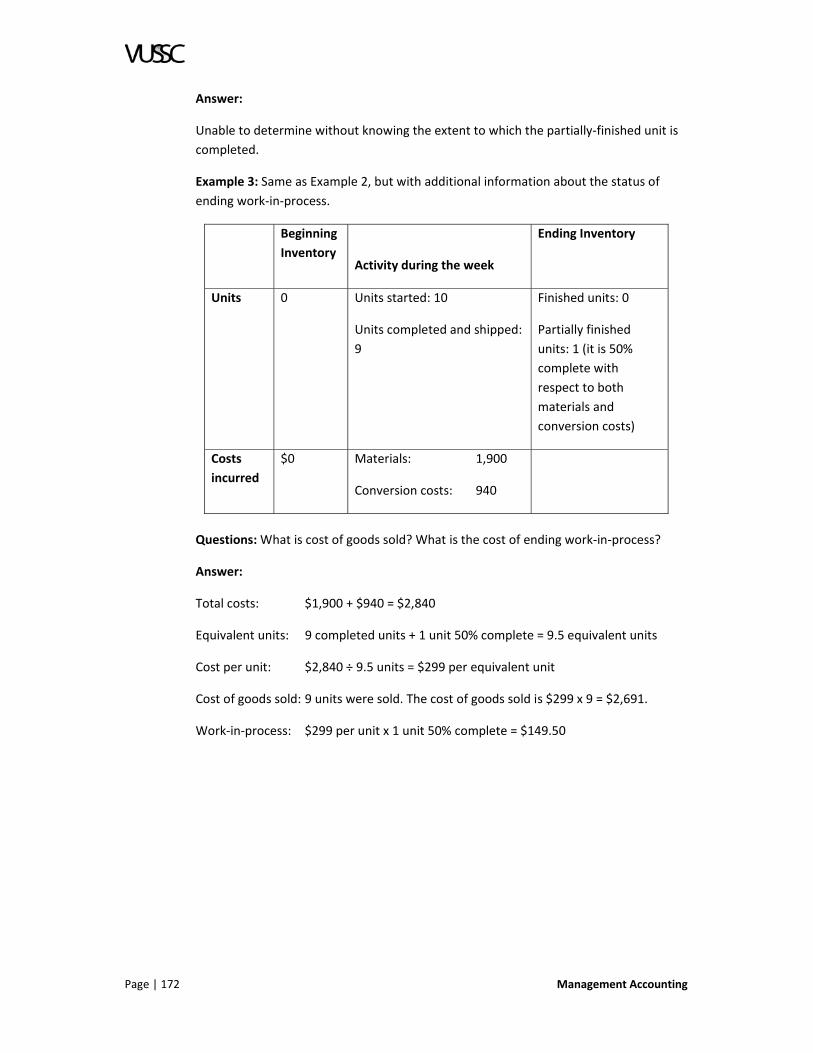
Page | 172 Management Accounting
Answer:
Unable to determine without knowing the extent to which the partially‐finished unit is
completed.
Example 3: Same as Example 2, but with additional information about the status of
ending work‐in‐process.
Beginning
Inventory
Activity during the week
Ending Inventory
Units 0 Units started: 10
Units completed and shipped:
9
Finished units: 0
Partially finished
units: 1 (it is 50%
complete with
respect to both
materials and
conversion costs)
Costs
incurred
$0 Materials:
Conversion costs:
1,900
940
Questions: What is cost of goods sold? What is the cost of ending work‐in‐process?
Answer:
Total costs: $1,900 + $940 = $2,840
Equivalent units: 9 completed units + 1 unit 50% complete = 9.5 equivalent units
Cost per unit: $2,840 ÷ 9.5 units = $299 per equivalent unit
Cost of goods sold: 9 units were sold. The cost of goods sold is $299 x 9 = $2,691.
Work‐in‐process: $299 per unit x 1 unit 50% complete = $149.50

Management Accounting Page | 173
Example 4: This example separates materials from conversion costs (labour and
overhead).
Beginning
Inventory
Activity during the week Ending Inventory
Units 0 Units started:
Units completed:
Units shipped
10
9
9
Finished units: 0
Partially finished units:
1
(it is 100% complete
with respect to
materials, 40%
complete with respect
to conversion costs.
Costs
incurred
$0 Materials:
Conversion Costs:
$1,900
940
Questions: What is cost of goods sold? What is the cost of ending work‐in‐process?
Answer:
Equivalent Units
Materials:
Conversion costs:
Cost per equivalent unit
Materials:
Conversion costs:
Total:
Cost of goods sold:
Work‐in‐process
Materials:
Conversion costs:
Total:
10 units (9 sold plus 1 unit in WIP 100% complete with
respect to materials)
9.4 units (9 sold plus 1 unit in WIP 40% complete with
respect to conversion costs)
$1,900 ÷ 10 equivalent units = $190 per equivalent unit
$940 ÷ 9.4 equivalent units = $100 per equivalent unit
$190 for materials + $100 for conversion costs = $290
$290 x 9 units sold = $2,610
$190 x 1 unit 100% complete = $190
$100 x 1 unit 40% complete = $40
$190 + $40 = $230
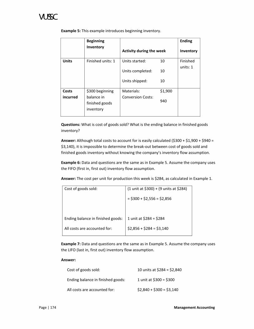
Page | 174 Management Accounting
Example 5: This example introduces beginning inventory.
Beginning
Inventory
Activity during the week
Ending
Inventory
Units Finished units: 1 Units started:
Units completed:
Units shipped:
10
10
10
Finished
units: 1
Costs
incurred
$300 beginning
balance in
finished goods
inventory
Materials:
Conversion Costs:
$1,900
940
Questions: What is cost of goods sold? What is the ending balance in finished goods
inventory?
Answer: Although total costs to account for is easily calculated ($300 + $1,900 + $940 =
$3,140), it is impossible to determine the break‐out between cost of goods sold and
finished goods inventory without knowing the company’s inventory flow assumption.
Example 6: Data and questions are the same as in Example 5. Assume the company uses
the FIFO (first in, first out) inventory flow assumption.
Answer: The cost per unit for production this week is $284, as calculated in Example 1.
Cost of goods sold:
Ending balance in finished goods:
All costs are accounted for:
(1 unit at $300) + (9 units at $284)
= $300 + $2,556 = $2,856
1 unit at $284 = $284
$2,856 + $284 = $3,140
Example 7: Data and questions are the same as in Example 5. Assume the company uses
the LIFO (last in, first out) inventory flow assumption.
Answer:
Cost of goods sold: 10 units at $284 = $2,840
Ending balance in finished goods: 1 unit at $300 = $300
All costs are accounted for: $2,840 + $300 = $3,140

Management Accounting Page | 175
Example 8: Data and questions are the same as in Example 5. Assume the company uses
the weighted average method for calculating cost of goods sold.
Answer: The weighted average method averages between the cost of goods on hand at
the beginning of the period, and the cost of goods produced during the period.
Total costs to account for:
Total equivalent units:
Cost per equivalent unit:
Cost of goods sold:
Ending balance in finished goods:
All costs are accounted for:
$3,140
1 unit from beginning inventory +
10 units made = 11 units
$3,140 ÷ 11 units = $285.45
10 units at $285.45 = $2,854.50
1 unit at $285.45 = $285.45
$2,854.50 + $285.45 = $3,140
Example 9: This example has partially finished units in both beginning inventory and
ending inventory. Assume the company uses the weighted average method.
Beginning Inventory Activity during the week Ending Inventory
Units 1 unit that is 50%
complete with
respect to both
materials and
conversion costs
The 1 unit coming into the
period is completed. 10 units
are started and completed. 1
unit is started but not
completed.
1 unit 20%
complete with
respect to both
materials and
conversion costs.
Costs
incurred
$150 beginning
balance in work‐in‐
process
Materials: Conversion
costs:
$1,900
940
Questions: What is the cost of each unit made? What is the cost of ending work‐in‐
process? If each unit completed is also sold, what is cost of goods sold?
Answer:
Total costs to account for:
Total equivalent units:
Cost per equivalent unit:
Ending work‐in‐process:
$150 + $1,900 + $940 = $2,990
11 units finished during the period plus one unit
that is 20% complete = 11.2 units
$2,990 ÷ 11.2 equivalent units = $266.96
$266.96 per unit x 1 unit 20% complete = $53.39

Page | 176 Management Accounting
Cost of goods sold: $266.96 x 11 units = $2936.56
Note: One might think that the calculation of equivalent units needs to include the
beginning inventory that is 50% complete. However, we would be double‐counting if we
did so, because the unit that is 50% complete in beginning inventory is one of the 11
units identified as finished during the period in the equivalent unit calculation. In the
schedule below, the costs to account for are highlighted in green, and the physical units
to account for are highlighted in yellow.
Beginning Inventory Activity during the week Ending Inventory
Units 1 unit 50% complete
with respect to both
materials and
conversion costs
The 1 unit coming into the period
is completed. 10 units are started
and completed. 1 unit is started
but not completed.
1 unit 20% complete
with respect to both
materials and
conversion costs.
Costs
incurred
$150 beginning
balance in WIP
Materials: Conversion
costs:
$1,900
940
LESSON PROBLEMS
Now review the following problems and answer the related questions. Record your
answers in your course workbook.
Problem 1
In applying the weighted‐average method for equivalent unit cost calculations, which of
the following information do you not need to know?
a. Production costs incurred during the period.
b. The equivalent units in beginning work‐in‐process inventory.
c. The cost of beginning work‐in‐process inventory.
d. All of the above must be known, in order to calculate the cost per equivalent
unit.
Problem 2
Part A ‐ Six units were in beginning work‐in‐process (WIP) at the beginning of May.
These units were 100% complete with respect to direct materials, and 50% complete
with respect to conversion costs. During the period, these six units were completed, and
another eight units were started. At the end of the period, four of these eight units
were completed, and the other four units were 100% finished with respect to direct
materials, and 75% complete with respect to conversion costs. Following is pertinent
cost information:
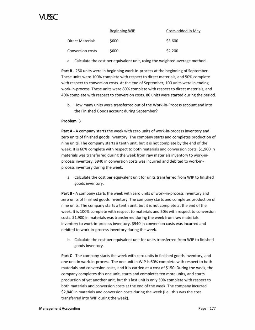
Management Accounting Page | 177
Beginning WIP Costs added in May
Direct Materials $600 $3,600
Conversion costs $600 $2,200
a. Calculate the cost per equivalent unit, using the weighted‐average method.
Part B ‐ 250 units were in beginning work‐in‐process at the beginning of September.
These units were 100% complete with respect to direct materials, and 50% complete
with respect to conversion costs. At the end of September, 100 units were in ending
work‐in‐process. These units were 80% complete with respect to direct materials, and
40% complete with respect to conversion costs. 80 units were started during the period.
b. How many units were transferred out of the Work‐in‐Process account and into
the Finished Goods account during September?
Problem 3
Part A ‐ A company starts the week with zero units of work‐in‐process inventory and
zero units of finished goods inventory. The company starts and completes production of
nine units. The company starts a tenth unit, but it is not complete by the end of the
week. It is 60% complete with respect to both materials and conversion costs. $1,900 in
materials was transferred during the week from raw materials inventory to work‐in‐
process inventory. $940 in conversion costs was incurred and debited to work‐in‐
process inventory during the week.
a. Calculate the cost per equivalent unit for units transferred from WIP to finished
goods inventory.
Part B ‐ A company starts the week with zero units of work‐in‐process inventory and
zero units of finished goods inventory. The company starts and completes production of
nine units. The company starts a tenth unit, but it is not complete at the end of the
week. It is 100% complete with respect to materials and 50% with respect to conversion
costs. $1,900 in materials was transferred during the week from raw materials
inventory to work‐in‐process inventory. $940 in conversion costs was incurred and
debited to work‐in‐process inventory during the week.
b. Calculate the cost per equivalent unit for units transferred from WIP to finished
goods inventory.
Part C ‐ The company starts the week with zero units in finished goods inventory, and
one unit in work‐in‐process. The one unit in WIP is 60% complete with respect to both
materials and conversion costs, and it is carried at a cost of $150. During the week, the
company completes this one unit, starts and completes ten more units, and starts
production of yet another unit, but this last unit is only 30% complete with respect to
both materials and conversion costs at the end of the week. The company incurred
$2,840 in materials and conversion costs during the week (i.e., this was the cost
transferred into WIP during the week).

Page | 178 Management Accounting
c. What is the cost of each unit transferred to finished goods inventory during the
week, using the weighted‐average method?
Problem 4
The factory started the period with 10 units. These units were 40% complete with
respect to materials, and 50% complete with respect to conversion costs. The cost of
this beginning WIP was $100 with respect to materials, and $70 with respect to
conversion costs. During the period the factory completed these 10 units, and started
production of another 6 units. Of the 6 units started during the period, 2 were finished,
and 4 were still in WIP at the end of the period. These 4 units were 50% complete with
respect to materials and 25% complete with respect to conversion costs. Manufacturing
costs incurred during the period were $2,700 for materials and $1,230 for conversion
costs.
a. Calculate the cost per equivalent unit using the weighted‐average method.
Problem 5
Part A ‐ In the mixing department, all the direct materials are added at the beginning of
the processing. Beginning work‐in‐process inventory consists of 2,000 units with a direct
materials cost of $31,860. During the period, 15,000 units are started and direct
materials costing $250,000 are charged to the department. If there are 1,000 units in
ending inventory, what is the cost per equivalent unit using the weighted‐average
method?
a. $15.93
b. $15.63
c. $14.83
d. $16.58
Part B ‐ The moulding department started 15,250 units in September and finished
16,625 units. If the ending work‐in‐process inventory was 500 units, what was the
beginning work‐in‐process inventory?
a. 875 units
b. 1,375 units
c. 2,375 units
d. 1,875 units
Part C ‐ Alex Company has 15,000 units in ending work‐in‐process inventory, which are
100% complete with respect to materials and 60% complete with respect to conversion
costs. The cost per unit for the month for materials is $3.00 and for conversion is $1.30.
What is the value of the ending work‐in‐process using the weighted‐average method?
a. $64,500
b. $38,700
c. $45,780

Management Accounting Page | 179
d. $56,700
Problem 6
The factory has zero beginning inventory, starts and completes 400 units, and starts
production of another 200 units, but these 200 units are not finished at the end of the
period. These 200 units are 50% complete with respect to materials, and 30% complete
with respect to labour and overhead. During the period, the factory spent $10,000 on
materials and $4,600 on labour and overhead.
a. Calculate the cost per equivalent unit using the weighted‐average method.
Problem 7
Kent Plastics began the period with 50 units that were 100% complete with respect to
materials and 50% complete with respect to conversion costs. During the period, Kent
began production of another 100 units. At the end of the period, there were 60 units,
100% complete with respect to materials and 50% complete with respect to conversion
costs.
a. Calculate the equivalent units produced during the period with respect to
conversion costs. (Note: This is not the denominator in the weighted‐average
method for determining the cost of production. Rather, it is a measure of the
level of production activity during the period.)
Problem 8
60 units were in beginning WIP. These units were 50% complete with respect to
materials and conversion costs. 50 units were in ending WIP. These units were also 50%
complete with respect to materials and conversion costs. During the period, 90 units
were transferred from WIP to Finished Goods.
a. How many units were started during the period?
Problem 9
VHI company started 2003 with 100 units in beginning work‐in‐process (WIP) that were
100% complete with respect to materials and 50% complete with respect to conversion
costs. The cost of this beginning WIP was $5,000 for materials and $3,000 for
conversion costs. During 2003, VHI complete these 100 units, and started another 100
units. At the end of 2003, VHI had 50 units in ending WIP that were 100% with respect
to materials and 10% complete with respect to conversion costs. VHI incurred materials
costs of $4,000 and conversion costs of $1,500 in 2003.
a. Compute the cost per equivalent unit using the weighted‐average method.
Problem 10
The factory has zero beginning inventory, starts and completes 100 units, and starts
production of another 200 units, but these 200 units are not finished at the end of the

Page | 180 Management Accounting
period. These 200 units are 100% complete with respect to materials, but only 50%
complete with respect to labour and overhead. During the period, the factory spent
$3,000 on materials and $8,000 on labour and overhead.
a. Calculate the cost per equivalent unit.
Problem 11
The factory started the period with 20 units on hand. These units were 100% complete
with respect to materials and 50% complete with respect to conversion costs. The
factory shipped 200 finished units to the warehouse. The factory ended the period with
40 units. These 40 units were 100% complete with respect to materials and 20%
complete with respect to conversion costs. Each unit requires one yard of fabric.
a. How many yards of fabric did the factory need to move from the storeroom to
the factory floor during the period (this is also the number of units started
during the period)?
LESSON SUMMARY
As noted in this lesson when calculating unit cost, it is often necessary to compute
equivalent units. When partially completed units are converted to whole units they are
referred to as equivalent units. It is important to know how much of your operating
costs are tied up in your inventory, including partially completed products. In the next
lesson we will explore other concepts important to managing inventory.
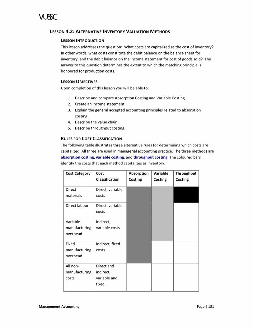
Management Accounting Page | 181
LESSON 4.2: ALTERNATIVE INVENTORY VALUATION METHODS
LESSON INTRODUCTION
This lesson addresses the question: What costs are capitalized as the cost of inventory?
In other words, what costs constitute the debit balance on the balance sheet for
inventory, and the debit balance on the income statement for cost of goods sold? The
answer to this question determines the extent to which the matching principle is
honoured for production costs.
LESSON OBJECTIVES
Upon completion of this lesson you will be able to:
1. Describe and compare Absorption Costing and Variable Costing.
2. Create an income statement.
3. Explain the general accepted accounting principles related to absorption
costing.
4. Describe the value chain.
5. Describe throughput costing.
RULES FOR COST CLASSIFICATION
The following table illustrates three alternative rules for determining which costs are
capitalized. All three are used in managerial accounting practice. The three methods are
absorption costing, variable costing, and throughput costing. The coloured bars
identify the costs that each method capitalizes as inventory.
Cost Category Cost
Classification
Absorption
Costing
Variable
Costing
Throughput
Costing
Direct
materials
Direct, variable
costs
Direct labour Direct, variable
costs
Variable
manufacturing
overhead
Indirect,
variable costs
Fixed
manufacturing
overhead
Indirect, fixed
costs
All non‐
manufacturing
costs
Direct and
indirect,
variable and
fixed.

Page | 182 Management Accounting
As the table indicates, non‐manufacturing costs are never capitalized as part of the cost
of inventory. The three methods differ with respect to their treatment of one or more
categories of manufacturing costs, but they all agree that non‐manufacturing costs
should not be debited as part of the cost of inventory.
For external financial reporting under Generally Accepted Accounting Principles, as well
as for tax reporting, companies are required to use absorption costing (also called full
costing). Hence, there is no choice from the above table for external financial reporting.
For internal reporting purposes, survey data suggests that approximately half of
manufacturing companies use absorption costing and approximately half use variable
costing. Throughput costing is a relatively recent phenomenon, and does not seem to
be used extensively yet.
ABSORPTION COSTING
The theoretical justification for absorption costing is to honour the matching principle
for all manufacturing costs. Fixed manufacturing overhead costs are only incurred with
the expectation that the resources represented by these costs will be used in the
production of inventory. Hence, these costs should be matched against the revenue
generated from the sale of that inventory.
Absorption costing requires computing an overhead rate for applying all manufacturing
overhead to units produced during the period (or else two overhead rates, one for
variable manufacturing overhead and one for fixed manufacturing overhead; or else
multiple overhead rates if the company uses activity‐based costing). There are
important issues related to choosing the denominator in the overhead rate for fixed
manufacturing overhead, which are discussed in the next Lesson of this book.
VARIABLE COSTING
The theoretical justification for variable costing is that fixed manufacturing overhead
(FMOH) will be incurred in the short‐run regardless of how much inventory is produced.
In many companies, even if a factory is idle, a significant portion of the FMOH is
unavoidable in the short run. For this reason, FMOH is treated as a period expense.
Variable costing used to be called direct costing with some frequency, but less so today.
Direct costing is a particularly confusing name, because the implication is that only
direct manufacturing costs are capitalized, whereas in fact, variable manufacturing
overhead is also capitalized. Even the name “variable costing” is perhaps less than ideal,
because not all variable costs are capitalized: non‐manufacturing costs are not
capitalized as part of the cost of inventory under any circumstances.
Under variable costing, the cost of ending inventory consists of direct manufacturing
costs (usually materials and labour) and variable manufacturing overhead. Hence, these
are the costs for which variable costing honours the matching principle, and nothing
else is capitalized as part of the cost of inventory.

Management Accounting Page | 183
ABSORPTION COSTING AND VARIABLE COSTING COMPARED
The only difference between absorption costing and variable costing is the treatment of
fixed manufacturing overhead (FMOH). Under absorption costing, FMOH is allocated to
units produced, so that there is a little bit of FMOH included in the cost of every unit of
inventory. Under variable costing, FMOH is treated as a period expense, appearing on
the income statement as a lump‐sum in the period incurred.
Comparing income under absorption costing to income under variable costing, the
following observations can be made:
1. When there are beginning and ending inventories, absorption costing and
variable costing will generally result in different inventory valuations for
beginning inventory, different inventory valuations for ending inventory, and
different incomes, but it is possible for the inventory balances and income to be
the same under the two methods.
2. If beginning and ending inventory levels are zero, absorption costing and
variable costing will always result in the same income.
3. If beginning inventory is zero and ending inventory is positive, absorption
costing will always result in higher income than variable costing, and a higher
valuation for ending inventory.
4. If beginning inventory is positive and ending inventory is zero, absorption
costing will always result in lower income than variable costing, and a higher
valuation for beginning inventory.
When inventory levels are increasing from period‐end to period‐end, as would be
expected when the company is growing, absorption costing will generally result in
higher ending inventory valuations than variable costing, and also higher income in each
period. The reason is that absorption costing postpones recognizing ever‐increasing
amounts of fixed manufacturing overhead on the income statement, because increasing
amounts of fixed manufacturing overhead are capitalized as ending inventory.
Over the life of the company (or from any point in time at which there is zero inventory
to any other point in time at which there is zero inventory), the sum of income over all
periods must be equal under the two methods. The difference between absorption
costing and variable costing is only a timing difference: the question of when fixed
manufacturing overhead is taken to the income statement.
INCOME STATEMENT PRESENTATION
Absorption costing, variable costing and throughput costing are each associated with an
income statement format:
Absorption costing uses a gross margin income statement, which starts with revenues
and subtracts cost of goods sold to derive gross margin, then subtracts non‐
manufacturing costs to derive operating income. Virtually every income statement
presented in connection with external financial reporting uses a gross margin format.
Gross margin income statements separate manufacturing costs from non‐
manufacturing costs, which is helpful for certain types of analyses.

Page | 184 Management Accounting
Variable costing uses a contribution margin income statement, which starts with
revenues and subtracts variable costs (variable manufacturing costs related to units
sold, plus all variable non‐manufacturing costs) to derive contribution margin, then
subtracts all fixed costs (manufacturing and non‐manufacturing) to derive operating
income. Contribution margin income statements facilitate cost‐volume‐profit analysis. It
should be emphasized that under variable costing, not all variable costs appear on the
income statement in the period incurred. Variable manufacturing costs that have been
incurred to make inventory that hasn’t been sold yet appear on the balance sheet as
part of the cost of finished goods inventory.
Throughput costing starts with revenues and subtracts direct material costs associated
with units sold to derive throughput margin, then subtracts all other costs.
These income statement formats do not define the costing methods. The costing
methods are defined by which manufacturing costs are capitalized, as indicated in the
table at the beginning of this Lesson. It is possible, for example, to cost inventory and
determine income using the rules of absorption costing, but to then present the data in
a contribution margin format by making certain reclassifications.
NUMERICAL EXAMPLE ‐ ABSORPTION COSTING AND VARIABLE COSTING
Following is information about the operations of Ultimate DNA, Inc., for the year ended
December 31, 2006.
Direct materials used in production
Direct labour costs incurred
Variable manufacturing overhead costs incurred
Variable non‐manufacturing costs incurred
Fixed manufacturing overhead costs incurred
Fixed non‐manufacturing costs incurred
$300,000
$100,000
$ 50,000
$ 40,000
$ 80,000
$ 20,000
There was no beginning inventory. 100 units were produced, and 50 units were sold at a
price of $20,000 per unit. The variable non‐manufacturing costs consist of two items: a
sales commission paid for units sold, and a transportation cost to ship finished product
from the factory to various warehouses where product is stored until it is sold.
Required: Prepare a Contribution Margin income statement, using Variable Costing.
Variable manufacturing costs:
In total: $300,000 materials + $100,000 labour + $50,000 variable O/H = $450,000
Per unit: $450,000 ÷ 100 units = $4,500 per unit

Management Accounting Page | 185
Ultimate DNA, Inc. Income Statement
For the Year Ended December 31, 2006
Sales
Variable Costs
Manufacturing ($4,500 per unit x 50 units)
Non‐manufacturing
Contribution Margin
Fixed Costs
Manufacturing
Non‐manufacturing
Operating Income
$1,000,000
225,000
40,000
735,000
80,000
20,000
$635,000
The only costs matched to revenues are the variable manufacturing costs. All other
costs are expensed as incurred.
Required: Prepare a Gross Margin income statement, using Absorption Costing.
Fixed and variable manufacturing costs:
In total: $450,000 variable (from above) + $80,000 fixed = $530,000
Per unit: $530,000 ÷ 100 units = $5,300 per unit
Ultimate DNA, Inc. Income Statement
For the Year Ended December 31, 2006
Sales
Manufacturing COGS ($5,300 per unit x 50 units)
Gross Margin
Non‐manufacturing Costs
Variable
Fixed
Operating Income
$1,000,000
265,000
735,000
40,000
20,000
$675,000
The matching principle is honoured for all manufacturing costs (fixed and variable), but
not for any of the non‐manufacturing costs.

Page | 186 Management Accounting
Required: Calculate the cost of ending inventory under Variable Costing.
$4,500 per unit x 50 units = $225,000
Only variable manufacturing costs are capitalized. All other costs are expensed as
incurred.
Required: Calculate the cost of ending inventory under Absorption Costing.
$5,300 per unit x 50 units = $265,000
Only manufacturing costs (fixed and variable) are capitalized. All non‐manufacturing
costs are expensed as incurred.
Under both Variable and Absorption Costing, all non‐manufacturing costs are expensed
as incurred. For example, the variable non‐manufacturing costs include a sales commis‐
sion for units sold, and a transportation cost incurred for all units shortly after they are
manufactured. Even though the transportation cost includes shipping costs for units in
the warehouse and not yet sold, this cost cannot be capitalized as part of the cost of
inventory, because the transportation cost is not a manufacturing cost, and inventory is
ready for sale at the time it leaves the factory.
ABSORPTION COSTING AND GENERALLY ACCEPTED ACCOUNTING PRINCIPLES
In 2004, the Financial Accounting Standards Board issued Statement of Financial
Accounting Standards (SFAS) No. 151, to amend and clarify generally accepted
accounting principles for the calculation of inventories under absorption costing. The
Board’s stated purpose for issuing the new standard was to improve the comparability
of cross‐border financial reporting, by aligning U.S. GAAP with the International
Accounting Standards Board’s Statement No. 2.
SFAS No. 151 was the first new pronouncement on absorption costing issued by a U.S.
accounting standard‐setting body in fifty years. Until SFAS No. 151, neither the Financial
Accounting Standards Board nor its predecessor, the Accounting Principles Board, had
specifically addressed absorption costing in a broad‐based way. Rather, each board had
incorporated GAAP that existed at the time the board was founded. Using this
genealogy, prior to SFAS No. 151, GAAP for absorption costing could be traced to
Accounting Research Bulletin (ARB) No. 43, issued in 1953 by the Committee on
Accounting Procedure (the predecessor to the Accounting Principles Board).
Key provisions of ARB No. 43, Lesson 4 on inventory pricing, included the following:
A major objective of accounting for inventories is the proper determination of income
through the process of matching appropriate costs against revenues.
‐ ARB No. 43, Lesson 2.2, Statement No. 2
As applied to inventories, cost means in principle the sum of the applicable
expenditures and charges directly or indirectly incurred in bringing an article to its
existing condition and location.

Management Accounting Page | 187
‐ ARB No. 43, Lesson 2.2, Statement No. 3
The definition of cost as applied to inventories is understood to mean acquisition and
production cost, and its determination involves many problems. … Under some
circumstances, items such as idle facility expense, excessive spoilage, double freight,
and re‐handling costs may be so abnormal as to require treatment as current period
charges rather than as a portion of the inventory cost.
‐ ARB No. 43, Lesson 2.2. Discussion of Statement No. 3
SFAS No. 151 amends ARB No. 43 by eliminating the “so abnormal” criterion in this last
paragraph. Hence, items such as idle facility expense and excessive spoilage must now
be recognized as current‐period charges.
With respect to idle facility expense, SFAS No. 151 requires fixed production overhead
to be allocated to inventory based on the “normal capacity” of the production facility.
The Statement defines normal capacity: “normal capacity refers to a range of
production levels, and is the production level expected to be achieved over a number of
periods or seasons under normal circumstances, taking into account the loss of capacity
resulting from planned maintenance.” The Statement notes that some variation in
production levels from period to period is expected, that normal capacity will vary
based on business‐specific and industry‐specific factors, and that these variations will
establish the range of normal capacity. Fixed manufacturing overhead can be allocated
based on the actual level of production when actual production approximates normal
capacity. The Statement observes that judgment is required to determine when a
production level is abnormally low (i.e., outside the range of the expected variation in
production). Examples of factors that might cause an abnormally low production level
include significantly‐reduced customer demand, labour and materials shortages, and
unplanned facility or equipment downtime.
Although SFAS No. 151 conveys the view of the Financial Accounting Standards Board
that the new pronouncement would not lead to significant changes in inventory
accounting practice, some companies’ financial statements may be affected. There is
some evidence that prior to SFAS No. 151, companies did not apply absorption costing
in the same manner. The vagueness in the wording of ARB No. 43 seemed to permit
alternative treatments. Furthermore, because ARB No. 43 did not require companies to
disclose how they applied absorption costing, information was generally not available
about the extent to which these alternative treatments were employed.
Survey data on this issue was provided in two articles that appeared in Management
Accounting by Michael Schiff (February 1987) and Steve Landekich (March 1973). These
surveys identify factory depreciation related to excess manufacturing capacity as an
example of fixed overhead that some but not all companies treated as a period
expense. Under SFAS No. 151, “The amount of fixed overhead allocated to each unit of
production is not increased as a consequence of abnormally low production or idle
plant.” Hence, if the survey data in Schiff and Landekich was still descriptive of practice
in 2004, some companies will have had to change their accounting treatment for idle

Page | 188 Management Accounting
capacity for inventory costs incurred during fiscal years beginning after June 15, 2005
(the effective date of SFAS No. 151).
Another area that Schiff and Landekich identified where companies differed in their
application of absorption costing is the decision of whether to allocate corporate
service department costs. Under ARB No. 43, the decision not to allocate these costs
seemed justified by materiality and expediency, rather than on theoretical grounds.
SFAS No. 151 states that under most circumstances, general and administrative
expenses should be included as period charges, except for the portion of such expenses
that may be clearly related to production. This wording seems to continue to allow
some latitude, and so companies might continue to differ in their treatment of these
costs.
THE VALUE CHAIN
The value chain is the sequence of activities that add value in a company. The following
table provides a typical list of activities in the value chain of a manufacturing firm,
although some manufacturers might outsource some of these activities.
Value Chain for a Manufacturing Firm
Research and development
Manufacturing
Marketing
Distribution
Sales
Customer service
For many industries, manufacturing costs constitute the majority of costs incurred in
the value chain. For companies in these industries, the decision to capitalize most or all
manufacturing costs as inventory, and to run these costs through the income statement
when the related inventory is sold, provides the benefits of the matching principle that
are discussed in introductory financial accounting courses.
However, there are some industries in which manufacturing costs are small relative to
one or more of the other activities in the value chain. For example, pharmaceutical
companies incur large research and development (R&D) costs. Under all three costing
methods that are discussed in this Lesson, R&D does not become a part of the cost of
inventory. In most situations, R&D is expensed when incurred for financial reporting
purposes, which clearly fails to honour the matching principle in a significant way. Large
expenditures are incurred and taken to the income statement for many years before
any revenue is realized for that drug, and then after the drug is approved by the Food
and Drug Administration, revenue is generated for many years with no directly‐related
offsetting R&D expenditures. The actual manufacturing cost of the drug can be quite
small relative to the R&D expenditures that were incurred to bring the drug to market.
Of course, the situation is somewhat more complicated for large pharmaceutical
companies, because there are numerous drugs at various stages in their lifecycles, so

Management Accounting Page | 189
that R&D on some projects offset revenue from drugs for which the R&D is already
complete, and also, there are many R&D projects that never result in a saleable
product.
Another industry in which manufacturing costs are small relative to some of the other
activities in the value chain is the soft drink industry. The ingredients and processes
used in the manufacture of soft drinks are fairly inexpensive, and there are few barriers
to entry. Consequently, soft drink companies spend large amounts on marketing and
advertising. These marketing efforts are anticipated to provide long‐term benefits by
turning consumers into life‐long Coca‐Cola® or Pepsi® drinkers. However, these costs are
not capitalized as part of the cost of inventory or as any other type of asset; rather, they
are expensed when incurred (subject to the usual accrual accounting practices).
THROUGHPUT COSTING
Also called super‐variable costing, throughput costing is a relatively new development.
Throughput costing treats all costs as period expenses except for direct materials. In
other words, the matching principle is honoured only for direct materials.
A company should probably meet two criteria before it chooses throughput costing. The
first criterion relates to the nature of the manufacturing process. Throughput costing
only makes sense for companies engaged in a manufacturing process in which most
labour and overhead are fixed costs. Assembly‐line and continuous processes that are
highly automated are most likely to meet this criterion. For example, thirty factory
employees might be required to work a given shift, regardless of whether the
machinery is set at full capacity or less. The second criterion is that management prefers
cost accounting information that is helpful for short‐term, incremental analysis, such as
whether the company should accept a one‐time special sales order at a reduced sales
price. In this respect, a company’s choice of throughput costing is a logical extension of
the company’s choice of variable costing over absorption costing.
Eliyahu Goldratt, who developed the theory of constraints, advocates throughput
costing in his popular business novel The Goal. Although throughput costing has not
gained wide acceptance, Goldratt’s support for it has been influential.
LESSON PROBLEMS
Now review the following problems and answer the related questions. Record your
answers in your course workbook.
Problem 1
Which of the following items account for the difference in income between Variable
Costing and Absorption Costing when inventory levels are changing? (Check all that
apply.)
a. Fixed manufacturing costs
b. Fixed non‐manufacturing costs
c. Variable manufacturing costs

Page | 190 Management Accounting
d. Variable non‐manufacturing costs
Problem 2
At a production level of 100 units, the per unit cost under Absorption Costing is $8,
which consists of $2 of direct materials, $2 of direct labour, $2 of variable
manufacturing overhead, and $2 of fixed manufacturing overhead.
a. Calculate the Absorption Costing per unit cost assuming the production level is
increased to 200 units?
Problem 3
Hank’s Hot Dog Factory manufactures hot dogs. The factory’s cost structure is as
follows: fixed manufacturing costs per month are $8,000. Variable manufacturing costs
are $0.40 per hot dog. Fixed non‐manufacturing costs are $7,000 per month. Variable
non‐manufacturing costs consist of a $0.20 sales commission for every hot dog sold.
The sales price per hot dog is $2.20.
a. If the company begins the month with zero inventory, makes 10,000 hot dogs,
and sells 7,000 hot dogs, what is the total cost of inventory on the Balance Sheet
at the end of the month under Variable Costing? What is income (loss) for the
month under Variable Costing?
Problem 4
The Esquimau Pie Company makes and sells the famous Esquimau Pie ice cream bar.
The company’s cost structure is as follows: fixed manufacturing overhead is $5,000
monthly. Variable manufacturing costs are $1.40 for each Esquimau Pie. Fixed non‐
manufacturing costs are $3,000 monthly. There are no variable non‐manufacturing
costs. The company begins the month with no inventory, makes 2,000 Esquimau Pies,
and sells 1,000 Esquimau Pies for $10 per pie.
a. What is the cost of ending inventory under Absorption Costing?
b. What is the cost of ending inventory under Variable Costing?
c. What is income under Absorption Costing?
d. What is income under Variable Costing?
Problem 5
The Impatients‐To‐Go Silk Flower Company began operations on January 1, 2004. Which
of the following circumstances ensures that the company’s net income will be the same
under Absorption Costing as under Variable Costing for 2005, its second year of
operations?
(I) The company has no inventory on January 1, 2005, and no inventory on December
31, 2005.
(II) The company incurred no fixed manufacturing overhead in 2005, and has no
inventory on December 31, 2005.

Management Accounting Page | 191
(III) The company incurred no fixed manufacturing overhead in 2004, and has no
inventory on December 31, 2005.
a. (I) only
b. (I) and (II) are each sufficient
c. (I) and (III) are each sufficient
d. (I), (II) and (III) are each sufficient
Problem 6
The Foster Company has variable and fixed manufacturing costs, and also some variable
and fixed non‐manufacturing costs. For the year 2005, the company has zero beginning
inventory, and positive ending inventory. Which statement is true?
a. Income in 2005 is the same under both Absorption Costing and Variable
Costing.
b. Income in 2005 is higher under Absorption Costing than under Variable Costing.
c. Income in 2005 is lower under Absorption Costing than under Variable Costing.
d. Unable to determine, from the information given, whether income is higher or
lower under Absorption Costing than under Variable Costing.
Problem 7
O’Brien and Hwang started 2006 with zero inventory, produced 100 units of product,
and sold 90 units. They incurred the following costs: variable manufacturing costs of
$10 per unit; fixed manufacturing costs of $2,000; variable non‐manufacturing costs of
a $2 sales commission per unit sold; and fixed non‐manufacturing costs of $700.
a. What will the 2006 year‐end balance sheet show for ending inventory if the
company uses Variable Costing?
b. Calculate net income for 2006 under Variable Costing. The sales price is $50 per
unit.
Problem 8
John Smith owned a flour mill. He started 1803 with no inventory, produced 50 tons of
flour, and ended the year with five tons of flour. Sales were $22,500. He had no variable
manufacturing overhead. His only direct cost was grain, for which he paid $8,000. Non‐
manufacturing variable costs were $5,000, non‐manufacturing fixed costs were $4,000,
and manufacturing fixed costs were $6,000.
a. What was Smith’s contribution margin for 1803?
1. $9,500
2. $10,300
3. $10,800
The answer depends on whether Smith uses Absorption Costing or Variable Costing
b. What was operating income for 1803 under Variable Costing?

Page | 192 Management Accounting
1. Loss of $500
2. Income of $800
3. Income of $900
4. Income of $300
Problem 9
The following information pertains to Booz Audio, a manufacturer of high‐end speakers
for home audio systems. Each “Unit” is actually two speakers (i.e., a pair of speakers).
The sales price per unit is $1,500 in both years. Beginning inventory in 2004 was zero.
2004
Units manufactured
Units sold
Direct manufacturing costs(materials and labour)
Variable manufacturing overhead
Fixed manufacturing overhead
Variable non‐manufacturing overhead
Fixed non‐manufacturing overhead
5,000
4,500
$2,000,000
500,000
1,000,000
50,000
100,000
2005
Units manufactured
Units sold
Direct manufacturing costs (materials and labour)
Variable manufacturing overhead
Fixed manufacturing overhead
Variable non‐manufacturing overhead
Fixed non‐manufacturing overhead
4,000
4,100
$1,600,000
400,000
1,000,000
40,000
100,000
a. Prepare a contribution margin income statement for 2005, using variable
costing, assuming the company uses FIFO.
b. Prepare a gross margin income statement for 2005, using absorption costing,
assuming the company uses FIFO.
c. Compute cost‐of‐goods‐sold for 2005, using absorption costing, assuming the
company uses LIFO.

Management Accounting Page | 193
Problem 10
The Arcata Bicycle Company began operations on January 1, 2000 with no inventory.
The company makes one product, a touring bike. Following is information for
production and sales for Arcata’s first two years of operations.
For the year
2000
For the year
2001
Units produced
Units sold
Selling price per unit
Direct materials per unit
Direct labour per unit
Sales commission per unit
100
85
$2,000
$100
$60
$20
100
80
$2,000
$90
$60
$20
In each year, total variable manufacturing overhead was $50,000; total fixed
manufacturing overhead was $60,000; and total fixed non‐manufacturing overhead was
$20,000. There were no variable non‐manufacturing costs other than sales
commissions.
a. How many units are in ending inventory at the end of 2001?
b. Using FIFO (First‐in First‐out) and Absorption Costing, what is the cost of ending
inventory on the Balance Sheet at the end of 2001?
c. Using Variable Costing and LIFO, what is income for 2001?
Problem 11
Onen Corporation makes just one product: a hydraulic pump that sells for $1,000 per
unit. In May, Onen started with zero units in beginning inventory, manufactured 400
pumps, and sold 350 pumps. The variable manufacturing cost is $600 per unit, which
consists of $300 in direct materials, $200 in direct manufacturing labour, and $100 in
variable manufacturing overhead. The fixed manufacturing overhead costs are $50,000.
The only variable non‐manufacturing cost is a warehousing fee incurred each time a
unit is manufactured, and this fee is $60 per unit. Fixed non‐manufacturing costs are
$70,000.
a. What will appear on the balance sheet at the end of May for the cost of ending
inventory under Variable Costing?
b. Prepare an income statement for May using Variable Costing. Use a
contribution margin format for the income statement.
c. What will appear on the balance sheet at the end of May for the cost of ending
inventory under Absorption Costing?
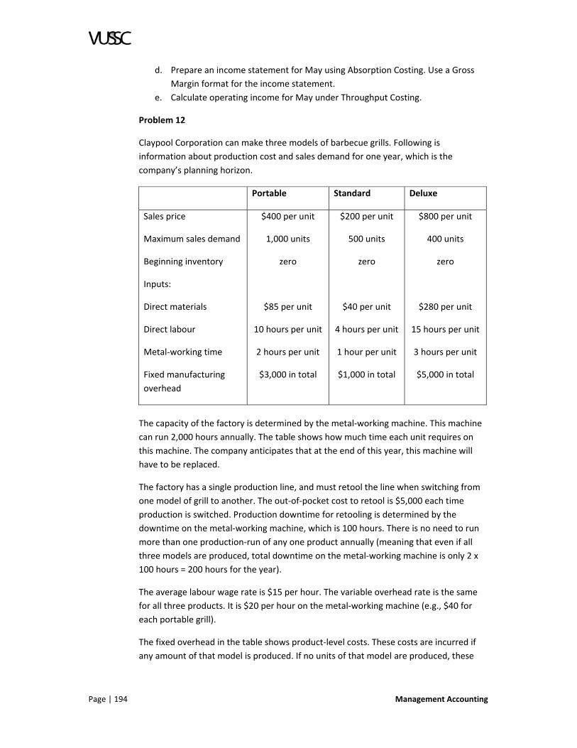
Page | 194 Management Accounting
d. Prepare an income statement for May using Absorption Costing. Use a Gross
Margin format for the income statement.
e. Calculate operating income for May under Throughput Costing.
Problem 12
Claypool Corporation can make three models of barbecue grills. Following is
information about production cost and sales demand for one year, which is the
company’s planning horizon.
Portable Standard Deluxe
Sales price
Maximum sales demand
Beginning inventory
Inputs:
Direct materials
Direct labour
Metal‐working time
Fixed manufacturing
overhead
$400 per unit
1,000 units
zero
$85 per unit
10 hours per unit
2 hours per unit
$3,000 in total
$200 per unit
500 units
zero
$40 per unit
4 hours per unit
1 hour per unit
$1,000 in total
$800 per unit
400 units
zero
$280 per unit
15 hours per unit
3 hours per unit
$5,000 in total
The capacity of the factory is determined by the metal‐working machine. This machine
can run 2,000 hours annually. The table shows how much time each unit requires on
this machine. The company anticipates that at the end of this year, this machine will
have to be replaced.
The factory has a single production line, and must retool the line when switching from
one model of grill to another. The out‐of‐pocket cost to retool is $5,000 each time
production is switched. Production downtime for retooling is determined by the
downtime on the metal‐working machine, which is 100 hours. There is no need to run
more than one production‐run of any one product annually (meaning that even if all
three models are produced, total downtime on the metal‐working machine is only 2 x
100 hours = 200 hours for the year).
The average labour wage rate is $15 per hour. The variable overhead rate is the same
for all three products. It is $20 per hour on the metal‐working machine (e.g., $40 for
each portable grill).
The fixed overhead in the table shows product‐level costs. These costs are incurred if
any amount of that model is produced. If no units of that model are produced, these
Management Accounting Page | 195
costs are completely avoidable. Facility‐level fixed manufacturing overhead costs are
$30,000 per year. These costs are unavoidable.
a. What is the most profitable product? Explain your reasoning.
b. What is the profit‐maximizing product mix? Assuming that the company uses
this product mix, show an income statement for each product produced.
c. Without regard to your answers to parts A and B, assume that the company
decides to produce only the portable heater. Halfway through the year, the
metal‐working machine breaks down, injuring the machine operator, and
prompting the labour union to call a strike. The machine cannot be repaired or
replaced for the rest of the year, and in any case, the workers remain on strike.
During the first six months, the company produced 500 portable heaters, and
by the end of the year, the company sold 400, leaving 100 units in ending
finished goods inventory. Value this ending inventory for financial reporting
purposes, in accordance with S.F.A.S. 151.
Problem 13
ZFN Scandinavia is a new affiliate of ZFN International. ZFN Scandinavia manufactures
bell‐bottom jeans in a single manufacturing facility. Following is pertinent data for 2005,
its first year of operations (hence, there is no beginning inventory).
Factory capacity: 250,000 jeans per year
Units manufactured in 2005: 192,000 jeans
Variable manufacturing costs: $10 per jean
Fixed manufacturing overhead costs: $1,344,000
S. G. & A. expenses: $2 per jean (this is a sales commission)
Sales: 150,000 jeans at $25 per jean
Sales demand, sales price, and variable costs are all expected to remain unchanged in
2006 from 2005. Fixed manufacturing overhead costs are expected to increase by 10%.
a. Calculate 2005 income and projected 2006 income under Absorption Costing,
under each of the following sets of assumptions:
The company accounts for inventory using FIFO, allocates fixed
manufacturing overhead costs based on units produced, manufactures
enough units in 2006 to plan for 60,000 units in ending inventory at the end
of the year.
The company accounts for inventory using FIFO, allocates fixed
manufacturing overhead costs based on units produced, manufactures at
capacity in 2006.
The company accounts for inventory using LIFO, allocates fixed
manufacturing overhead costs based on units produced, manufactures

Page | 196 Management Accounting
enough units in 2006 to plan for 60,000 units in ending inventory at the end
of the year.
The company accounts for inventory using LIFO, allocates fixed
manufacturing overhead costs based on units produced, manufactures at
capacity in 2006.
b. Calculate 2005 income and projected 2006 income under Variable Costing,
under FIFO, assuming the company manufactures enough units in 2006 to plan
for 60,000 units in ending inventory at the end of the year.
Problem 14
Aztech Industries makes only one product. In 2001, the company started the year with
zero beginning inventory. The company reported the following results for 2005 and
2006:
2005 2006
Units made
Units sold
Average unit sales price
Variable manufacturing costs
Fixed overhead manufacturing costs
Variable non‐manufacturing costs
Fixed non‐manufacturing costs
20
18
$1,000
$1,400
$3,500
$ 180
$ 900
10
7
$1,000
$ 700
$3,500
$ 90
$ 900
a. How many units are in ending inventory at the end of 2006?
b. Calculate the cost of ending inventory at the end of 2006, assuming the
company uses Absorption Costing, and the FIFO (first‐in, first‐out) inventory
flow assumption.
c. Calculate operating income for 2006, assuming the company uses Absorption
Costing, and the LIFO (last‐in, first‐out) inventory flow assumption.
d. Calculate operating income for 2006, using either FIFO or LIFO (whichever you
prefer), assuming the company uses Variable Costing.
e. Calculate the cost of ending inventory at the end of 2006, assuming the
company uses Variable Costing, using either FIFO or FIFO (whichever you
prefer).
f. Assume the company uses Absorption Costing. What is the Gross Margin in
2005?
g. Assume the company uses Variable Costing. What is the contribution margin
(i.e., the total contribution margin) for 2005?
Management Accounting Page | 197
Problem 15
A factory has fixed manufacturing overhead of $10,000,000 per year. Production
capacity (practical capacity) is 20,000 units per year. The normal range of production,
for purposes of SFAS No. 151, ranges from 12,000 units to 18,000 units annually. In the
past, the company had always used actual production to calculate the fixed cost per
unit. The company uses the FIFO inventory flow assumption. The company started the
year with 3,000 units, produced 10,000 units, and sold 11,000 units.
a. How much more income or less income will the company show this year under
SFAS No. 151 than it would have shown under its old method of allocating fixed
manufacturing overhead, assuming that the company uses the flexibility
permitted under SFAS No. 151 to minimize the effect of this new
pronouncement on its financial statements relative to its old accounting?
Assume that this is the first year the company implements SFAS No. 151, and
assume the pronouncement is implemented prospectively, so beginning
inventory is not restated.
Problem 16
A factory has fixed manufacturing overhead of $10,000 per month. Practical capacity is
2,000 units per month. The normal range of production, for SFAS No. 151, ranges from
1,200 units to 1,800 units monthly. In the past, the company used practical capacity to
calculate the fixed cost per unit, and recorded the volume variance in COGS. The
company uses LIFO. The company started the month with 1,000 units, produced 1,200
units, and sold 1,300 units.
a. How much more income or less income will the company show this month
under SFAS No. 151 than it would have shown under its old method of
allocating fixed manufacturing overhead, assuming that the company uses the
midpoint of the range of normal capacity in the denominator of its fixed
overhead rate? Assume that this is the first month the company implements
SFAS No. 151, and assume the pronouncement is implemented prospectively,
so that inventory produced in prior months and brought into the current month
as beginning inventory is not restated.
The answer is zero. Since the company is on LIFO, and since current month sales exceed
current month production, all fixed manufacturing overhead incurred this month is
expensed this month, either as part of Cost of Goods Sold or as the volume variance.
Problem 17
In July, Border Industries made 1,000 units of its sole product, and sold 800 units. There
were no beginning inventories. Its net income for the month using Variable Costing was
$20,000. Its net income for the month using Absorption Costing was $24,000. Its
contribution margin for the month was $50,000, and its gross margin for the month was
also $50,000. Sales revenue for the month was $200,000. Border is on an actual costing

Page | 198 Management Accounting
system (i.e., overhead is allocated using a rate and allocation base that are based on
actual amounts). There are no fixed direct costs.
a. How much fixed manufacturing overhead was incurred during the month?
b. How much fixed non‐manufacturing overhead was incurred during the month?
c. What was the per unit variable manufacturing cost for the month?
d. What was the total variable non‐manufacturing costs incurred during the
month?
e. What is the cost of ending inventory under Absorption Costing?
f. What is the cost of ending inventory under Variable Costing?
Problem 18
Copernicus International uses Variable Costing, and the weighted‐average inventory
flow assumption. The company started the period with zero finished goods and 100
units of work‐in‐process. These units were 30% complete with respect to materials and
70% complete with respect to labour and variable manufacturing overhead. The cost of
this beginning work‐in‐process was $10,000 in materials and $40,000 in labour and
variable manufacturing overhead. During the period, the company completed these 100
units and started production of another 50 units. At the end of the period, of the 50
units started during the period, 20 were finished, and 30 were 20% complete with
respect to materials and 50% complete with respect to labour and variable
manufacturing overhead. Manufacturing costs incurred during the period were $8,000
for materials and $32,000 for labour and variable manufacturing overhead. Fixed
manufacturing overhead for the period was $75,000. Fixed non‐manufacturing costs
were $10,000. Variable non‐manufacturing costs were a $20 sales commission per unit
sold. 85 units were sold, at an average sales price of $2,000 per unit.
a. Prepare a Contribution Margin format income statement for the period.
b. What are the balances in the work‐in‐process and finished goods inventory
accounts at the end of the period?
LESSON SUMMARY
As we learned in this lesson inventory cost is the cost of holding goods in stock. It is
expressed as percentage of the inventory value. The inventory cost includes the capital,
warehousing, depreciation, insurance, taxation, obsolescence, and shrinkage costs.
Inventory is merchandise that is purchased by the merchandisers to be sold to the
customers. The cost of the inventory that is bought but not yet sold is reported in the
account inventory or Merchandise Inventory. Inventory costs are costs associated with
the producing of a product that are capitalized in the inventory. They become assets
until they are sold.
In the next lesson we will explore the impact of fixed overhead costs on the operation
of a business.

Management Accounting Page | 199
LESSON 4.3: FIXED MANUFACTURING OVERHEAD
LESSON INTRODUCTION
In this lesson we will discuss the calculation and application of a fixed manufacturing
overhead. This form of applied overhead represents the fixed manufacturing costs
(e.g., property tax, rent, and depreciation on factory) that have been assigned to
(absorbed by) the products manufactured via a predetermined rate. Ideally, by the end
of the accounting year the amount applied will equal the amount actually incurred.
LESSON OBJECTIVES
Upon completion of this lesson you will be able to:
1. Explain alternative denominator levels.
2. Identify production incentives.
3. Describe the impact of allocating of fixed overhead on management decision‐
making.
REVIEW
If you recall the steps to product costing include:
1. Identify the cost object;
2. Identify the direct costs associated with the cost object;
3. Identify overhead costs;
4. Select the cost allocation base for assigning overhead costs to the cost object;
5. Develop the overhead rate per unit for allocating overhead to the cost object.
This lesson will focus on steps #3 through #5 for fixed manufacturing overhead.
WHAT ARE ALTERNATIVE DENOMINATOR LEVELS?
It is possible to allocate overhead separately for fixed overhead and for variable
overhead, and there are sometimes good reasons to do so. When fixed and variable
manufacturing overhead is allocated separately, there are important issues related to
how the denominator of the fixed overhead rate is calculated. Alternative denominator
choices include:
1. Theoretical Capacity: This measure of factory capacity assumes 100% efficiency
100% of the time. It is analogous to the EPA miles‐per‐gallon estimates that are
determined for new automobiles; nobody actually achieves this gas mileage in
day‐to‐day driving, but the EPA estimates are useful for comparison shopping.
2. Practical Capacity: This measure of factory capacity reduces theoretical
capacity for anticipated unavoidable operating interruptions, including routine
maintenance.
3. Normal Capacity: This denominator‐level concept measures the level of factory
activity that satisfies average customer demand over an intermediate period of
time. It frequently averages over seasonal or cyclical fluctuations in demand. As

Page | 200 Management Accounting
discussed in the previous Lesson, Generally Accepted Accounting Principles now
require companies to allocate fixed production overhead based on the “normal
capacity” of the production facilities for external financial reporting purposes.
The definition of normal capacity provided here is similar in concept to the
definition provided in SFAS No. 151, although the definition in the
pronouncement provides some latitude and encompasses a range of production
levels.
4. Budgeted Production: This denominator‐level concept has been introduced
previously. It is the level of factory activity budgeted for the upcoming period.
Because fixed costs, by definition, do not depend on the level of output, the numerator
in the fixed overhead rate is not expected to differ across these four denominator
choices. Since there is no cause‐and‐effect relationship in the short run between the
estimation of the numerator and the quantity of the allocation base in the
denominator, the larger the denominator, the smaller the amount of fixed overhead
costs that are allocated to each unit of product.
This situation contrasts with variable overhead. In fact, for variable overhead, the
numerator cannot be estimated until the denominator is estimated. For example, an
apparel factory cannot accurately estimate electricity expense for the coming year until
it predicts the amount of time the machines will run, and this estimate depends on the
projected level of production. Hence, for variable overhead, the allocation base is
chosen, then the quantity of the allocation base is estimated, and then variable
overhead costs are estimated.
PRODUCTION INCENTIVES
Many accounting writers have emphasized the effect that the allocation of fixed
overhead can have on managerial incentives to overproduce. When fixed overhead is
allocated to product, the greater the production level, the lower the fixed cost per unit.
The lower fixed cost per unit might increase perceived profitability, but is the company
really more profitable?
The answer to this question depends on what happens to the additional inventory. If
the company is producing more inventory than it can sell, and is consequently
stockpiling finished goods inventory, then clearly the company is not more profitable.
This situation arises in Eliyahu Goldratt’s business novel The Goal (co‐authored with Jeff
Cox). Factory management in the novel is so committed to maximizing output and
minimizing per‐unit production cost, that they rent a warehouse to store large
quantities of excess inventory.
On the other hand, if the factory can sell all of the goods that it produces, then as
production increases, the factory really does become more profitable. Furthermore,
when fixed costs are allocated to product, this increased profitability is reflected in the
lower per‐unit cost.
Management Accounting Page | 201
The key question, then, is whether managers, companies, or factories with incentives to
overproduce can stockpile inventory without negative repercussions. It would seem
that in the business environment of the past several decades, this risk has been
overrated. Excess inventory is highly visible, physically and on the balance sheet, both
for managerial accounting and financial reporting purposes. Hence, while it is important
for managers and management accountants to be aware that the allocation of fixed
overhead can provide incentives to overproduce, the risk posed by these incentives
probably need not dictate the decision of whether to allocate fixed overhead for
management accounting purposes. (Recall from Lesson 15 that for financial accounting
purposes, companies must allocate fixed manufacturing overhead.)
THE ALLOCATION OF FIXED OVERHEAD AND MANAGEMENT DECISION‐MAKING
A more difficult question than perverse production incentives is whether the allocation
of fixed overhead assists or hinders sourcing, marketing and pricing decisions. This
question, which can be characterized as a debate of the merits of absorption costing
versus contribution margin analysis, has probably generated more controversy than any
other issue in management accounting. Following are three views from prominent
accounting faculty.
In the second edition of his textbook Managerial Accounting (copyright 2004), James
Jiambalvo, Dean of the Business School at the University of Washington, states that the
major limitation of activity‐based costing is that most companies use ABC to develop
the full cost of products (Lesson 6, p. 208). Jiambalvo also offers only one answer to the
question of why GAAP requires absorption costing: that “company managers may be
concerned that variable cost information will prove helpful to competitors” (Lesson 5, p.
169). It is clear from these statements and others in his textbook that Professor
Jiambalvo perceives little benefit from absorption costing for managerial decision‐
making.
Robert Kaplan, Professor at Harvard University, participated in a Panel Discussion on
contribution margin analysis at the Annual Meeting of the American Accounting
Association. Professor Kaplan, who was one of the most persuasive early advocates of
activity‐based costing and one of the originators of the Balanced Scorecard (discussed in
Lesson 24), commented:
Interestingly, many companies have resisted for the most part the attempts
by academic accountants to convince them to ignore their fixed costs. …
Most companies persist in performing full cost allocations.
Journal of Management Accounting Research, 1990 (Fall), p. 4
In fact, surveys suggest that for internal reporting purposes, approximately 50% of
companies use variable costing and 50% use absorption costing.
In 1989, John Shank participated in the same panel discussion as Bob Kaplan. Professor
Shank’s comments included the following:
Page | 202 Management Accounting
I now believe at the broadest possible level that my [former] support for the
contribution margin concept was misplaced and short‐sighted. … I have been
looking for some big successes from contribution margin analysis for 25
years, and I have come up empty. … In fact, it almost seems to be axiomatic,
and let me call it Shank’s Axiom.
If the problem is small enough so that contribution margin analysis is
relevant then it can’t have a very big impact on a company.
And if the possible impact in a decision setting is major, if it can really affect
a company in a major way, then it’s silly to consider most of the factors to be
fixed.
… Not only can I find no notable big successes from contribution margin
concepts in the real world, I can point to many examples of what I consider
to be notable failures from the application of the contribution margin mind‐
set. … I believe that more than one entire industry has competed itself to the
brink of insolvency using contribution‐based pricing.
Journal of Management Accounting Research, 1990 (Fall), p. 17
Professor Shank refers to the trucking and airline industries in the years following their
deregulation as two examples to illustrate his point. If an airplane is about to leave the
gate with empty seats, the marginal cost of adding additional passengers to fill those
seats is almost zero (a small increase in fuel consumption, and a few bags of pretzels,
perhaps). Hence, an airline applying contribution margin analysis will make every effort
to try to fill the plane to capacity, including offering deeply‐discounted, last‐minute
fares. However, it is an open question as to whether the numerous bankruptcies and
near‐bankruptcies that have occurred in the airline industry in the years following
deregulation resulted from a “contribution margin mind‐set,” as Professor Shank
suggests, or rather from the underlying economic characteristics of the industry. Given
overcapacity in the industry, the fact that airlines have high fixed costs and low variable
costs, and the fact that airlines have difficulty differentiating the services that they offer
from their competitors, it is not clear that any one airline would have improved its
situation using a full costing approach to pricing.
EXAMPLE ‐ ANNIE’S SOUP COMPANY
The following fictional example illustrates the general nature of the debate between
contribution margin analysis and absorption costing.
Annie’s Soup Company manufactures twelve types of soup in its facility in Eureka,
California. Each soup is produced on its own equipment, in a portion of the facility
dedicated exclusively to it. The facility is running at 70% of capacity.
Annie’s Soup Company has traditionally reported the full cost of products for internal
performance evaluation purposes, allocating facility‐level costs to each product based
on machine hours. Annie’s philosophy is to encourage product managers to set sales

Management Accounting Page | 203
prices that will support the company’s overall profit targets, and she believes that full
costing supports this objective. If facility‐level costs were not allocated, then each
product might show a profit, yet the company as a whole could show a loss.
The product manager of the cream soup line has proposed a new product: a cream
spinach soup that would be called Annie’s Ultimate Spinach soup. The product manager
admits that initial demand for this product probably would not support a sales price
that would cover the full cost of the product including an allocation of facility‐level
costs. However, the product manager convinces Annie that because the facility has
excess capacity, the new soup should be required to meet only its marginal costs (unit‐
level, batch‐level and product‐level costs in the cost hierarchy, but not facility‐level
costs). At a sales price of $1.75 per can to retailers, without an allocation of facility‐level
costs the profit margin would be $0.25 per can, but with facility‐level costs allocated to
Ultimate Spinach soup, it would be projected to show a loss of $0.25 per can.
The product manager’s argument persuades Annie to approve the production of
Ultimate Spinach soup, and to evaluate it, at least initially, based on a cost that excludes
facility‐level costs.
The following year, the product manager of the tomato‐based soups proposes a new
tomato bisque soup. She asserts that since the latest soup introduced by the cream
soup manager does not have facility‐level costs allocated to it, neither should her new
tomato bisque. Annie agrees.
Three years pass. The situation is now as follows. The company has 14 soups. Twelve
soups have facility‐level costs allocated to them, two do not. Is this situation acceptable,
and if not, what should be done about it?
The current situation seems problematic. Annie cannot directly compare profitability
across all 14 soups. As time passes, and as the date each soup was introduced becomes
less salient, it is increasingly difficult to view Annie’s Ultimate Spinach Soup and the
Tomato Bisque as the “marginal products.” In any case, as discussed in Caplan,
Melumad and Ziv (The Denim Finishing Company, Issues in Accounting Education, 2005),
it is not at all clear that contribution margin analysis can be effectively applied by always
treating the newest product as the marginal product.
Should Annie start allocating facility‐level overhead to all 14 products? If so, there is no
obvious point in time at which to initiate this allocation to the two new products.
Furthermore, if one of the new products shows a loss when facility‐level costs are
allocated to it, and if the factory still has excess capacity, it is not clear that the
unprofitable product should be dropped. Marginal cost analysis applied to the decision
of whether to drop a product is as relevant now as the initial marginal cost analysis that
supported introducing the product in the first place.
Should Annie stop allocating facility‐level overhead to all 14 products, and convert to a
variable costing approach to product profitability analysis? The disadvantage of this
approach is that without an allocation of facility‐level costs, each of the 14 products

Page | 204 Management Accounting
could generate a positive contribution margin, which might be viewed positively by
each of the product managers, yet the company as a whole could still be unprofitable.
Rather, full costing helps ensure that product managers attempt to set sales prices that
support the company’s overall profitability goals.
LESSON PROBLEMS
Now review the following problems and answer the related questions. Record your
answers in your course workbook.
Problem 1
The Taos Ski and Tennis Resort has a Summer manager and a Winter manager. These
managers receive a substantial portion of their income in the form of a bonus based on
profitability. They constantly argue about how certain costs should be allocated across
the two seasons. For example, they both wanted a new espresso bar constructed, and
they convinced the owner to build it by agreeing to have the construction cost
depreciated over the life of the building, and to have each year’s depreciation expense
allocated between the Summer season and the Winter season for purposes of
calculating each manager’s profits. This convinced the owner that the managers really
believed the espresso bar would cover its costs. However, although the two managers
agreed that these fixed costs should be allocated, and although they believe that the
incremental revenue will more than cover the costs, including the cost to build the
espresso bar, they can’t agree on how to allocate depreciation expense between the
two seasons. The summer manager suggests splitting depreciation expense 50/50, since
the number of visitors is about the same for each season. The Winter manager suggests
splitting depreciation expense 70/30 (70% to Summer), since this roughly represents
the length (in days) of each season.
The best way for the owner to resolve this dispute is to:
a. Not allocate depreciation expense at all, since the cost of the building was
relevant before it was built, but is irrelevant now that it is a sunk cost.
b. Allocate depreciation 50/50, since all else equal, this will not favor either
manager.
c. Allocate depreciation 70/30, because this method is consistent with
depreciating the entire cost of the building over its useful life.
d. Allocate the cost based on actual espresso bar revenues, since this allocates
costs on an “ability to bear” basis, and recognizes the fact that guests are more
likely to buy coffee when the weather is cooler, so that the Summer manager is
not penalized.
Problem 2
The Bernalillo Tortilla Factory manufactures a variety of packaged Mexican food
products in a large factory in Northern New Mexico. In general, each product has its
own equipment, factory personnel, and product manager. Many of these products are

Management Accounting Page | 205
currently very popular, and in the short‐term, there is not enough space in the factory
to meet consumer demand. Which of the follow statements are true?
a. Allocating fixed manufacturing overhead to production will encourage product
managers to set sales prices on individual products that will help achieve the
company’s overall profitability goals.
b. Allocating fixed manufacturing overhead to production using factory square feet
as the allocation base will assist management in determining the most profitable
product mix.
c. Allocating fixed manufacturing overhead to production during the year will
provide product cost information that is more consistent with the company’s
year‐end financial statements (prepared in accordance with Generally accepted
Accounting Principles) than would treating fixed manufacturing overhead as a
period expense.
d. Fixed manufacturing overhead costs are sunk in the short‐run, and hence, are
independent of the level of production. Therefore, there is no purpose in
allocating these costs to production.
Problem 3
Milwood Mills makes decorative woodcut prints. Each design is run in a single batch
once during the year. Milwood Mills allocates machine set‐up costs using set‐up hours
as the allocation base. Following is budgeted information for next year for two of the
company’s numerous designs: Bull and Matador and Dogs Playing Poker.
Bull Dogs
Number of woodcuts
Direct materials cost
Direct labour cost
Number of machine set‐up hours
Pounds of material
Kilowatt hours
5,000
$25,000
$14,000
120
5,000
2,000
15,000
$33,000
$16,000
150
10,000
3,000
a. What is the anticipated effect of making the 5,000 “Bull” woodcuts in two
batches instead of one, holding all else constant, if machine set‐up costs are
variable, in a linear fashion, in the number of setups?
1) The unit cost of “Bull” will increase, and the unit cost of “Dogs” will
decrease.
2) The unit cost of “Bull” will increase, and the unit cost of “Dogs” will
remain unchanged.

Page | 206 Management Accounting
3) The unit cost of “Bull” will decrease, and the unit cost of “Dogs” will
remain unchanged.
4) The unit cost of both “Bull & Matador” and “Dogs” will remain
unchanged.
b. What is the anticipated effect of making the 5,000 woodcuts of “Bull” in two
batches instead of one, holding all else constant, if machine set‐up costs include
both fixed and variable components?
1) The unit cost of “Bull” will increase, and the unit cost of “Dogs” will
decrease.
2) The unit cost of “Bull” will increase, and the unit cost of “Dogs” will
remain unchanged.
3) The unit cost of “Bull” will decrease, and the unit cost of “Dogs” will
remain unchanged.
4) The unit cost of both “Bull & Matador” and “Dogs” will remain
unchanged.
Problem 4
The not‐for‐profit health clinic Shots‐Я‐Us provides various types of vaccinations and
other shots, especially flu shots, to the public for free or for a nominal fee. The clinic is
funded by several local governmental agencies as well as by a number of charitable
organizations. Since different donors wish to fund different types of shots, the clinic
determines the full cost of each type of shot, by adding overhead to the direct costs,
and then provides this information to current and prospective donors.
Following are actual and budgeted costs for Shots‐Я‐Us for 2003:
Actual Budgeted
Number of patient visits
Number of shots administered
Fixed overhead: salaries, rent for the facility,
insurance, depreciation.
Variable overhead: nursing staff hourly wages,
utilities, disposable supplies.
Cost of hypodermics (a direct cost)
Cost of medications (a direct cost)
5,000
6,000
$94,000
$66,000
$1,000
$30,000
4,000
4,500
$110,000
$40,500
$750
$20,000
Assume the clinic allocates fixed overhead separately from variable overhead, and
allocates fixed overhead using the number of shots as the allocation base. Clinic
management believes that the facility could deliver as many as 7,000 shots per year.

Management Accounting Page | 207
Which of the following overhead rates will result in under allocated fixed overhead for
the year?
I. Actual level of activity in the denominator, and actual costs in the numerator.
II. Budgeted level of activity in the denominator, and budgeted costs in the numerator.
III. Practical capacity in the denominator, and budgeted costs in the numerator.
a. III only
b. II and III only
c. II only
d. I only
e. neither I, II, nor III
Problem 5
The Carl‐Carlson Corporation uses Absorption Costing, begins the year with zero
inventory, and has both fixed and variable manufacturing costs. Relative to the
benchmark in which the company produces the same number of units that it sells,
which of the following statements is true?
a. By producing above its sales level, the company will increase the total cost of
ending inventory on the balance sheet, and will also increase net income.
b. By producing above its sales level, the company will increase the total cost of
ending inventory on the balance sheet, but will not affect net income.
c. By producing above its sales level, the company will increase the total cost of
ending inventory on the balance sheet, but will decrease net income.
d. None of the above statements can be made with certainty, unless the actual
costs and unit volumes are known.
Problem 6
For the year 2004 (his first year of operations), Harvey Mudd sold 7,500 units at $350
per unit, and produced 10,000 units, of his sole product, a combination espresso
machine and rug steamer. Factory capacity is 15,000 units. Other information for the
year included the following:
Direct manufacturing labour
Variable manufacturing overhead
Direct materials
Variable selling expense (a sales commission)
Fixed non‐manufacturing expenses
Fixed manufacturing overhead
$750,000
400,000
600,000
400,000
400,000
800,000

Page | 208 Management Accounting
On January 1, 2005, Harvey predicts that his sales demand and cost structure (total
fixed cost and variable cost per unit) will remain exactly the same in 2005 as it was in
2004. Harvey doesn't want to change his sales price, uses FIFO for financial reporting,
and wants to show the same profits under Variable Costing as under Absorption Costing
in 2005.
a. Is there an attainable production level that will accomplish this goal? If so, what
is that production level?
Problem 7
For the year 2049, its first year of operations, Montgomery Scott Enterprises sold 7,500
units at $350 per unit, and produced 10,000 units, of its sole product, a Shuttlecraft
navigational device. Other information for the year included:
Direct manufacturing labour
Variable manufacturing overhead
Direct materials
Variable selling expenses
Fixed administrative expenses
Fixed manufacturing overhead
$750,000
400,000
600,000
400,000
400,000
800,000
On January 1, 2050, Scott uses a new software program, Econ‐forecast, which predicts
that his sales demand and cost structure will remain exactly the same in 2050 as it was
in 2049. Scott doesn’t want to change his sales price, uses LIFO for financial reporting,
and wants to show zero profits (i.e., wants to break even) in 2050.
a. Is there a production level under absorption costing that will accomplish this
goal?
b. If so, what is it?
Problem 8
The Eureka Company began operations on January 1, 2005 with no inventory. The
company makes one product, an electric lawn mower. Following is information for
production and sales for 2005, and projected information for 2006:
Actual for
2005
Projections for 2006
Units produced
Units sold
190
100
To be determined (by you)
210

Management Accounting Page | 209
Actual for
2005
Projections for 2006
Selling price per unit
Direct materials per unit
Direct labour per unit
Variable non‐manufacturing costs:
Sales commission per unit
$2,500
$190
$70
$40
$2,600
$220
$70
$45
Factory capacity is 200 units per year. In 2005, total variable manufacturing overhead
was $85,500; total fixed manufacturing overhead was $200,000; and total fixed non‐
manufacturing overhead was $30,000. There were no variable non‐manufacturing costs
other than the sales commissions. The total fixed costs and the per‐unit variable
overhead costs are expected to be the same in 2006 as in 2005. The company uses LIFO
(Last‐in, First‐out) and Absorption Costing.
a. Prepare a Gross Margin format income statement for 2005.
b. Is there a production level for 2006 that will allow the company to earn profits
of $100,000 in 2006, if all goes according to plan? If so, what is that production
level?
Problem 9
The Well‐Managed Manufacturing Company is concerned about how much income it
will report for the year ending December 31, 2006. It is now mid‐November, and the
estimated (pro forma) income statement for the year, calculated on a Variable Costing
basis, is as follows:
Sales
Variable costs:
Manufacturing costs
Selling and administrative costs
Contribution margin
Fixed costs:
Manufacturing costs
Selling and administrative costs
Operating income
50,000 units
$200,000
100,000
$300,000
100,000
$750,000
300,000
$450,000
400,000
$ 50,000

Page | 210 Management Accounting
Well‐Managed began the year with zero inventory and was anticipating ending the year
with zero inventory. However, the managers have been promised a bonus if income is
at least $100,000 calculated according to Generally Accepted Accounting Principles.
One of the managers wants to increase income by increasing production, even though
the level of sales for the year will not be affected.
a. What is the cost per unit of inventory, and operating income, using Absorption
Costing, assuming the company has no inventory at year‐end, as planned?
b. How much inventory would have to be produced for ending inventory, in order
to raise income to $100,000?
c. In other words, what would the balance in ending inventory have to be?
d. One manager believes that producing unneeded inventory to generate income
is a bad idea. What do you think?
LESSON SUMMARY
Understanding overhead costs and how to identify them is important part of a business
financial plan. Overhead rates for each department within your company must be
calculated based on the services they need to support their portion of the business.
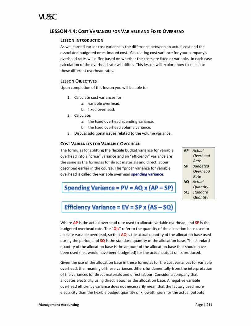
Management Accounting Page | 211
LESSON 4.4: COST VARIANCES FOR VARIABLE AND FIXED OVERHEAD
LESSON INTRODUCTION
As we learned earlier cost variance is the difference between an actual cost and the
associated budgeted or estimated cost. Calculating cost variance for your company’s
overhead rates will differ based on whether the costs are fixed or variable. In each case
calculation of the overhead rate will differ. This lesson will explore how to calculate
these different overhead rates.
LESSON OBJECTIVES
Upon completion of this lesson you will be able to:
1. Calculate cost variances for:
a. variable overhead.
b. fixed overhead.
2. Calculate:
a. the fixed overhead spending variance.
b. the fixed overhead volume variance.
3. Discuss additional issues related to the volume variance.
COST VARIANCES FOR VARIABLE OVERHEAD
The formulas for splitting the flexible budget variance for variable
overhead into a “price” variance and an “efficiency” variance are
the same as the formulas for direct materials and direct labour
described earlier in the course. The “price” variance for variable
overhead is called the variable overhead spending variance:
Where AP is the actual overhead rate used to allocate variable overhead, and SP is the
budgeted overhead rate. The “Q’s” refer to the quantity of the allocation base used to
allocate variable overhead, so that AQ is the actual quantity of the allocation base used
during the period, and SQ is the standard quantity of the allocation base. The standard
quantity of the allocation base is the amount of the allocation base that should have
been used (i.e., would have been budgeted) for the actual output units produced.
Given the use of the allocation base in these formulas for the cost variances for variable
overhead, the meaning of these variances differs fundamentally from the interpretation
of the variances for direct materials and direct labour. Consider a company that
allocates electricity using direct labour as the allocation base. A negative variable
overhead efficiency variance does not necessarily mean that the factory used more
electricity than the flexible budget quantity of kilowatt hours for the actual outputs
AP
SP
AQ
SQ
Actual Overhead Rate Budgeted Overhead Rate Actual Quantity Standard Quantity
Page | 212 Management Accounting
produced. Rather, the negative variance literally means that the factory used more
direct labour than the flexible budget quantity for direct labour. If there is a cause‐and‐
effect relationship between the allocation base and the variable overhead cost category
(i.e., if more direct labour hours implies more electricity used), then the negative
efficiency variance suggests that more electricity was used than the flexible budget
quantity, but the efficiency variance does not measure kilowatts directly.
Similarly, a negative spending variance for variable overhead does not necessarily mean
that the cost per kilowatt‐hour was higher than budgeted. Rather, a negative spending
variance for variable overhead literally states that the actual overhead rate was higher
than the budgeted overhead rate, which could be due either to a higher cost per
kilowatt‐hour, or more kilowatt hours used per unit of the allocation base. Hence, what
one might think should be included in the efficiency variance (kilowatt hours required
per direct‐labour‐hour being higher or lower than budgeted) actually gets included as
part of the spending variance.
COST VARIANCES FOR FIXED OVERHEAD
Whereas the cost variances for direct materials, direct labour, and variable overhead all
use the same two formulas, the cost variances for fixed overhead are different, and do
not use these formulas at all.
Also, whereas cost variances for direct materials, direct labour, and variable overhead
can be calculated for individual products in a multi‐product factory, cost variances for
fixed overhead can only be calculated for the factory or facility as a whole. (More
precisely, fixed overhead cost variances can only be calculated for the combined
operations to which the resources represented by the fixed costs apply.)
There are two fixed overhead cost variances: the spending variance and the volume
variance.
The Fixed Overhead Spending Variance
The fixed overhead spending variance is the difference between two lump sums:
Actual fixed overhead costs incurred Budgeted fixed overhead costs
The fixed overhead spending variance is also called the fixed overhead price variance or
the fixed overhead budget variance.
The Fixed Overhead Volume Variance
The fixed overhead volume variance is also called the production volume variance,
because this variance is a function of production volume. The volume variance attaches
a dollar amount to the difference between two production levels. The first production
level is the actual output for the period. The second production level is the
denominator‐level concept in the budgeted fixed overhead rate, expressed in units. As
discussed in the previous Lesson, there are two common choices for this denominator:

Management Accounting Page | 213
budgeted production
factory capacity
The interpretation of the volume variance depends on which of these two
denominators are used, but in either case, the production volume variance is the
difference between budgeted fixed overhead (a lump sum), and the amount of fixed
overhead that would be allocated to production under a standard costing system using
this fixed overhead rate.
The volume variance with budgeted production in the denominator of the O/H rate:
First we use budgeted production to calculate the volume variance. In this case:
The term in parenthesis equals the amount of fixed overhead that would be allocated to
production under a standard costing system, when budgeted production is the
denominator‐level concept.
Since:
Budgeted fixed overhead ÷ budgeted production = budgeted overhead rate
the above expression for the volume variance is algebraically equivalent to the
following formula:
This formula for the volume variance illustrates the statement above; that the volume
variance attaches a dollar amount to the difference between two production levels. In
this case, the two production levels are actual production and budgeted production.
The interpretation of the volume variance, when budgeted production is used in the
denominator of the overhead rate, is the following. When actual production is less than
budgeted production, the volume variance represents the fixed overhead costs that are
not allocated to product because actual production is below budget. In this case, the
volume variance is unfavourable. When actual production is greater than budgeted
production, then the volume variance represents the additional fixed overhead costs
that are allocated to product because actual production exceeds budget. In this case,
the volume variance is favourable.
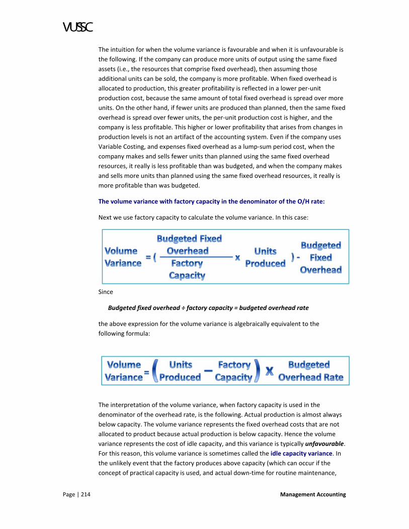
Page | 214 Management Accounting
The intuition for when the volume variance is favourable and when it is unfavourable is
the following. If the company can produce more units of output using the same fixed
assets (i.e., the resources that comprise fixed overhead), then assuming those
additional units can be sold, the company is more profitable. When fixed overhead is
allocated to production, this greater profitability is reflected in a lower per‐unit
production cost, because the same amount of total fixed overhead is spread over more
units. On the other hand, if fewer units are produced than planned, then the same fixed
overhead is spread over fewer units, the per‐unit production cost is higher, and the
company is less profitable. This higher or lower profitability that arises from changes in
production levels is not an artifact of the accounting system. Even if the company uses
Variable Costing, and expenses fixed overhead as a lump‐sum period cost, when the
company makes and sells fewer units than planned using the same fixed overhead
resources, it really is less profitable than was budgeted, and when the company makes
and sells more units than planned using the same fixed overhead resources, it really is
more profitable than was budgeted.
The volume variance with factory capacity in the denominator of the O/H rate:
Next we use factory capacity to calculate the volume variance. In this case:
Since
Budgeted fixed overhead ÷ factory capacity = budgeted overhead rate
the above expression for the volume variance is algebraically equivalent to the
following formula:
The interpretation of the volume variance, when factory capacity is used in the
denominator of the overhead rate, is the following. Actual production is almost always
below capacity. The volume variance represents the fixed overhead costs that are not
allocated to product because actual production is below capacity. Hence the volume
variance represents the cost of idle capacity, and this variance is typically unfavourable.
For this reason, this volume variance is sometimes called the idle capacity variance. In
the unlikely event that the factory produces above capacity (which can occur if the
concept of practical capacity is used, and actual down‐time for routine maintenance,

Management Accounting Page | 215
etc., is less than expected), then the volume variance represents the additional fixed
overhead costs that are allocated to product because actual production exceeds
capacity. In this case, the volume variance is favourable.
ISSUES RELATED TO THE VOLUME VARIANCE
Under what circumstances would a company calculate the volume variance using
budgeted production as the denominator‐level concept, and under what circumstances
would a company use factory capacity as the denominator‐level concept?
The use of budgeted production in the calculation of the volume variance attaches a
lump sum benefit or cost to actual production levels that exceed or fall short of
budgeted production levels. For this reason, many companies consider this calculation
of the volume variance to be an important performance measure for the factory
manager and marketing managers responsible for making and marketing the product.
The use of factory capacity in the calculation of the volume variance provides an
indication of how low the per‐unit cost can go, if demand equals or exceeds factory
capacity. If senior management would like product managers to make pricing and
operating decisions based on a long‐term expectation that demand for the product will
equal or exceed factory capacity, even though current or short‐term demand is below
capacity, calculating the per‐unit cost in this manner will encourage product managers
to take this long‐run perspective. For example, consider the launch of a new product
line in a new factory. If fixed overhead is allocated based on budgeted production, then
product managers might feel pressured to set sales prices that will cover full product
costs at initially‐low production levels, but these sales prices might be too high to
generate sufficient initial consumer interest in the product for a successful product
launch.
Another reason to use factory capacity in the denominator of the fixed overhead rate,
and in the calculation of the volume variance, is that doing so isolates the cost of idle
capacity. Often, the decision to build a factory that is larger than current demand
warrants is a strategic decision made at high levels within the organization. If the fixed
overhead associated with this factory is allocated based on budgeted or actual
production, the per‐unit cost of every unit manufactured includes a small portion of the
cost of this strategic decision, and the cost reports of factory managers and the product
profitability statements of product managers are negatively affected by this unused
capacity. Some companies prefer to isolate the cost associated with this strategic
decision, and to either show the cost of idle capacity as separate line‐items on the cost
reports and profit statements of the factory manager and product managers, or remove
this cost entirely from these performance reports, and report it only at the corporate
level.
Allocating fixed overhead using actual production can provide managers short‐run
incentives to overproduce, because as production increases, the per‐unit cost
decreases. Similarly, calculating the volume variance using budgeted production in the
denominator of the overhead rate can provide managers short‐run incentives to

Page | 216 Management Accounting
overproduce, because as production exceeds budget, the volume variance becomes
increasingly favourable. For this reason, some companies choose not to allocate fixed
overhead at all. However, the use of factory capacity in the denominator of the fixed
overhead rate accomplishes the same objective, because it isolates the volume variance
such that the performance reports of these managers need not be affected by it.
We have assumed, throughout this section, that fixed overhead is allocated based on
units of output. However, we saw in the Lesson on activity‐based costing that units of
production is often a poor choice of allocation base in a multi‐product factory, and
many companies that use standard costing systems use allocation bases that are more
sophisticated, such as direct labour hours or direct materials dollars. The question might
arise, how does the use of a different allocation base, such as direct labour hours, affect
the calculation of the volume variance? The answer is: Not at all. Because of the way in
which standard costing systems work, the amount of fixed overhead that will be
allocated to product does not depend on the choice of allocation base.
For example, assume that a one‐product company budgets two direct labour hours to
make each unit, and assume that if fixed overhead is allocated based on output units,
the budgeted fixed overhead rate is $10 per unit. Then using direct labour hours as the
allocation base, the budgeted fixed overhead rate is $5 per direct labour hour. Because
of the mechanics of standard costing systems, no matter whether the $10‐per‐unit rate
is used, or the $5‐per‐direct‐labour‐hour rate is used, $10 of fixed overhead will be
allocated to every unit produced, no matter how many direct labour hours are actually
used per unit. (If this fact is not obvious to you, refer back to Lesson 10 on standard
costing.) Therefore, for the purpose of calculating the volume variance, we might as
well use the easiest allocation base, which is units‐of‐output.
It is important to recognize that even though most manufacturing companies use a
standard costing system and even though the calculation of the fixed overhead volume
variance relies on the concept of standard costing, companies can calculate the volume
variance even if they do not use a standard costing system. In this case, the calculation
is identical to the discussion above, but the company will not be able to obtain the
required information from the cost accounting system itself, but rather, will need to
make a separate calculation.
EXAMPLE ‐ FIXED OVERHEAD VARIANCES
The Coachman Company makes pencils. The pencils are sold by the box. Following is
information about the company’s only factory:
Budget Actual Capacity
Number of boxes Direct labour hours Machine hours Fixed overhead
10,000200500
$40,000
12,000250650
$42,000
20,000

Management Accounting Page | 217
The outputs here are boxes of pencils. The inputs are direct labour hours and machine
hours. First we calculate a fixed overhead rate using actual amounts, and output units
as the allocation base:
$42,000 ÷ 12,000 boxes = $3.50 per box.
Using this overhead rate, every box of pencils is costed at the variable cost of
production plus $3.50 in allocated fixed overhead.
Next: we calculate a fixed overhead rate using budgeted costs, and budgeted output
units as the denominator‐level concept:
$40,000 ÷ 10,000 boxes = $4.00 per box.
Next: we calculate a fixed overhead rate using budgeted costs, and factory capacity as
the denominator‐level concept (expressed in terms of output units).
$40,000 ÷ 20,000 boxes = $2.00 per box.
The advantage of using capacity in the denominator is that this denominator‐level
concept shows how low the fixed cost per unit can go, and hence, how low the total
cost per unit can go, as production increases.
The fixed overhead spending variance is calculated as follows:
$42,000 actual $40,000 budgeted = $2,000 unfavourable.
Next: we calculate the volume variance using capacity as the denominator‐level
concept:
volume variance = ($2.00 per box x 12,000 boxes) $40,000 = $16,000 unfavourable
or equivalently:
volume variance = $2.00 per box x (12,000 boxes 20,000 boxes) = $16,000 unfavourable
If the company uses a standard costing system, the amount of over allocated or under
allocated fixed overhead is the difference between actual fixed overhead incurred, and
fixed overhead allocated to product, calculated as follows:
actual fixed overhead fixed overhead allocated
= $42,000 ($2.00 per box x 12,000 boxes)
= $42,000 $24,000 = $18,000 under allocated
This $18,000 of under allocated fixed overhead is equal to the sum of the $2,000
unfavourable fixed overhead spending variance and the $16,000 unfavourable volume
variance.

Page | 218 Management Accounting
Next: we calculate the volume variance using budgeted production as the denominator‐
level concept:
volume variance = ($4.00 per box x 12,000 boxes) $40,000 = $8,000 favourable
or equivalently:
volume variance = $4.00 per box x (12,000 boxes 10,000 boxes) = $8,000 favourable
If the company uses a standard costing system, the amount of over allocated or under
allocated fixed overhead is the difference between actual fixed overhead incurred, and
fixed overhead allocated to product, calculated as follows:
actual fixed overhead fixed overhead allocated
= $42,000 ($4.00 per box x 12,000 boxes)
= $42,000 $48,000 = $6,000 over allocated
This $6,000 of over allocated fixed overhead is equal to the sum of the $2,000
unfavourable fixed overhead spending variance (which did not change when we
changed the denominator‐level concept from capacity to budgeted production) and the
$8,000 favourable volume variance.
To illustrate that the choice of allocation base does not affect the calculation of the
volume variance, we recalculate the volume variance assuming the company allocates
overhead using machine hours as the allocation base and budgeted production as the
denominator‐level concept. The budgeted overhead rate is now
$40,000 ÷ 500 machine hours = $80 per machine hour.
Since the standard for machine time is one hour for every twenty boxes (derived from
the budget column in the box at the beginning of the example), the standard costing
system will allocate fixed overhead as follows:
Budgeted overhead rate x (standard inputs allowed for actual outputs achieved)
= $80 per machine hour x (12,000 boxes ÷ 20 boxes per machine hour)
= $80 per machine hour x 600 machine hours = $48,000
And the volume variance is:
fixed overhead allocated to product budgeted fixed overhead
= $48,000 $40,000 = $8,000 favourable, as before.

Management Accounting Page | 219
LESSON PROBLEMS
Now review the following problems and answer the related questions. Record your
answers in your course workbook.
Problem 1
Following is selected information about the Hopi Popcorn company. All information
represents total amounts, not per unit amounts.
Static Budget Actual
Results
Units made and sold
Direct materials costs
Direct materials used in
production
Fixed overhead
100
$5,000
1,000 pounds
$3,000
50
$2,700
450 pounds
$4,000
Hopi had no beginning or ending inventory of either finished product or raw materials.
Hopi allocates fixed overhead using units of output as the allocation base, and a
budgeted overhead rate with budgeted production in the denominator.
a. Calculate the fixed overhead volume variance.
Problem 2
Assume the following information for the Centerville 2 plant of Polypar, which
manufactures only butyl.
Budgeted fixed overhead
Plant production capacity
Budgeted butyl production
Actual butyl production
$12,000,000
1,000,000 tons of butyl
500,000 tons of butyl
600,000 tons of butyl
a. Using budgeted butyl production in the denominator of the fixed overhead rate,
calculate the fixed overhead volume variance.
b. Using plant capacity in the denominator of the fixed overhead rate, calculate the
fixed overhead volume variance.
c. In one or two sentences, interpret what each of these variances represents.
Page | 220 Management Accounting
Problem 3
Yellow Company budgeted fixed manufacturing overhead of $1,000,000, but actually
incurred fixed manufacturing overhead of $1,200,000. The company expected to
produce 100,000 units of product, but actually produced 80,000 units. The company
allocates fixed overhead using a budgeted rate, based on budgeted production in the
denominator.
a. Calculate the fixed overhead spending variance. Is this variance favourable or
unfavourable?
b. Calculate the fixed overhead volume variance. Is this variance favourable or
unfavourable?
c. Calculate the over allocated or under allocated fixed overhead.
Problem 4
The Plutonium Fruitcake Company allocated variable overhead based on pounds of
direct materials. The company's production level (units of output) and direct materials
prices (cost per pound) in 1957 were exactly as planned in the static budget for that
year, but the company used more pounds of direct materials per unit of output than
planned. This set of circumstances certainly resulted in
I. an unfavourable variable overhead efficiency variance.
II. an unfavourable flexible budget variance for variable overhead.
III. an unfavourable static budget variance for variable overhead.
a. (I), (II) and (III)
b. neither (I), (II) nor (III) need be true
c. (I) only
d. (I) and (II) only
Problem 5
Following is information about December production at the Doorstop Fruitcake
Company, and the principal ingredient used in the manufacture of fruitcakes: flour. All
flour purchased during the month was used in production. There was no flour on hand
at the beginning of the month. Fixed manufacturing overhead was budgeted at $90,000,
but was actually $100,000. Fixed manufacturing overhead is allocated using pounds of
flour as the allocation base. The factory expects to be operating at capacity in
December.
# of Fruitcakes
produced
Pounds of
flour used
Cost of
flour
Actual
Budget
1,150
1,200
5,980
6,000
$2,840.50
$3,000.00

Management Accounting Page | 221
If the company allocates variable overhead based on pounds of flour, the variable
overhead efficiency variance will be:
a. Zero
b. Unfavourable
c. Favourable
d. Unable to determine from the information provided
Problem 6
Which of the following scenarios might not result in an unfavourable production volume
variance?
I. Actual production is below practical capacity, when budgeted production is used in
the denominator to calculate the overhead rate.
II. Actual production is below practical capacity, when practical capacity is used in the
denominator to calculate the overhead rate.
III. Actual production is below budget, when budgeted production is used in the
denominator to calculate the overhead rate.
IV. Actual production is above budget, when practical capacity is used in the
denominator to calculate the overhead rate.
a. I and IV
b. I only
c. I, II, III and IV
d. I and III
Problem 7
Assume the following information for the Pittsfield factory of Carnegie Steel.
Budgeted fixed overhead
Production capacity
Budgeted production
$12,000,000
1,000,000 tons
500,000 tons
a. Assume we are at the beginning of the year. If the volume variance will be
calculated using plant capacity in the denominator of the fixed overhead rate,
what would the plant manager have to do to ensure that the production volume
variance will be zero?
b. Again, assume we are at the beginning of the year. If the volume variance will be
calculated using budgeted production in the denominator of the fixed overhead
rate, what would the plant manager have to do to ensure that the production
volume variance will be favourable?

Page | 222 Management Accounting
c. Assume that we are at the beginning of the year, and that the factory manager is
told that the production volume variance, favourable or unfavourable, will be
recorded at the corporate level, and not on the factory income statement that
forms the basis for the manager’s performance review. Assume also that the
factory manager is given the choice of the denominator‐level concept for
calculating the volume variance (actual, budget, or practical capacity), but that
the manager must make the choice at the beginning of the year, knowing only
the information in the table at the start of this question, but not knowing actual
production or actual fixed overhead costs.
1. What denominator‐level concept do you think the factory manager will
choose, and why?
2. Would your answer change if, instead of budgeting production of
500,000 tons, production was budgeted for factory practical capacity
of 1,000,000 tons?
Problem 8
If a factory is on a Standard Costing System, and has over allocated fixed overhead,
which of the following statements is certainly true?
a. The factory made more units than planned.
b. The factory has a favourable spending variance.
c. The factory has a favourable production volume variance.
d. The actually amount spent for fixed overhead was less than the amount of fixed
overhead allocated to inventory.
Problem 9
The Large and Expensive Widget Company allocates overhead based on direct labour
hours. If the company uses more total direct labour hours than planned, but the actual
labour wage rate is the same as the budgeted labour wage rate, which of the following
statements might not be true?
a. There will be an unfavourable static budget variance for labour.
b. The labour wage rate variance will be zero.
c. There will be an unfavourable labour efficiency variance.
d. The labour efficiency and overhead efficiency variances will be in the same
direction (i.e., either both variances will be favourable, they will both be
unfavourable, or they will both be equal to zero).
Problem 10
McConnell McDowell McQueen Enterprises makes cotton shirts in a single factory in
Cold Spring, VT. The company uses a Standard Costing System. The company allocates
fixed and variable overhead separately. Variable overhead is allocated using direct
labour hours as the allocation base. Fixed overhead is allocated based on output units
(i.e., the allocation base is shirts), and factory practical capacity is the denominator‐level

Management Accounting Page | 223
concept. Practical capacity is 2,000 shirts per month. Following is budgeted and actual
information for the month.
Static Budget
Information
Actual
Results
Production
Number of shirts
Direct Materials
Cost per yard of fabric
Yards of fabric per shirt
Direct labour
Direct labour cost for all of the shirts
Hours of direct labour for all of the shirts
Variable Overhead
Fixed Overhead
1,200
$4.50
2.00
$27,000
3,000
$18,000
$15,000
1,000
$4.20
2.50
$30,000
3,400
$18,500
$10,500
a. Calculate the spending and efficiency variances for variable overhead.
b. Compute the fixed overhead volume variance. Is it favourable or unfavourable?
c. Compute the spending variance for fixed overhead.
d. Compute the amount of under allocated or over allocated fixed overhead.
Problem 11
Li, Lee and Levy Industries make widgets in its factory located in the Marina Shores
district of Seattle. The company uses a standard costing system. Following is budgeted
and actual information for the month.
Static Budget
Information
Actual Results
Widgets produced
Direct materials: copper fibres
Direct labour
1,000
15,000 pounds for a
total cost of $31,500
1,000 hours for a total
cost of $9,000
900
12,600 pounds for a
total cost of $25,200
950 hours for a total
cost of $8,075

Page | 224 Management Accounting
Static Budget
Information
Actual Results
Variable overhead (allocated
based on machine hours)
Fixed costs (allocated based on
units of output, and budgeted
production in the denominator)
Machine hours
$18,000
$56,000
800
$14,553
$57,000
630
a. Calculate the variances for variable and fixed overhead.
Problem 12
NPX Company reports the following information for October:
Static Budget Actual Results
Production
Direct labour
Variable overhead
Fixed overhead
Machine hours
1000 units
20 minutes per unit
$3,333
$47,000
200
1,100 units
15 minutes per unit
$3,666
$47,000
220
NPX allocates overhead based on direct labour hours, using a standard costing system,
and allocates fixed overhead using the denominator‐level concept of budgeted
production.
a. How much of the flexible budget variance for variable overhead is due to the
fact that NPX produced more units than planned?
b. The variable overhead efficiency variance is $917 favourable (rounded to the
nearest dollar). Recalculate the variable overhead efficiency variance assuming
the company allocates overhead based on machine hours instead of labour
hours.
c. Calculate the variable overhead spending variance assuming the company
allocates variable overhead based on machine hours instead of labour hours.
d. Calculate the fixed overhead spending variance. Is it favourable or
unfavourable?
e. How much of the fixed overhead spending variance is due to the fact that
production was higher than planned?
f. Calculate the fixed overhead volume variance.

Management Accounting Page | 225
g. How much of the fixed overhead volume variance is due to the fact that
production was higher than planned?
h. Calculate the amount of over applied or under applied fixed overhead.
Problem 13
The Electric Sound Opera Company makes three models of an electronic keyboard.
Budgeted and actual information for the year follows:
Model A
Model B
Model C
Total
Units produced: actual budgeted
Direct materials (per unit) actual budgeted
Direct labour (per unit) actual budgeted
Cost driver info: number of parts (per unit)
actual budget
direct labour hours (per unit) actual budget
total square feet (budget = actual) Overhead costs: Labour Support (variable overhead)
actual budget
Materials Support (variable overhead) actual budget
Fixed Overhead actual budget
Total Overhead actual budget
315275
$50$52
$24$20
3232
3.504
3,000
450400
$76$73
$56$50
5656
4.605
6,000
226 300
$100 $105
$38 $40
43 43
4.50
5 10,000
991975
19,000
$ 535,000$ 600,000
$ 780,000$ 860,000
$1,250,000$1,000,000
$2,565,000$2,460,000
Notes:
1. The company uses a Normal Costing System.
2. Total square feet refers to the square feet of factory floor space used in the
production of each model of product. It is expressed as total square feet for that
model, not square feet per unit.
3. Variable manufacturing overhead is divided into two cost pools, one for labour
support and one for materials support.

Page | 226 Management Accounting
a. Assume that the Labour Support overhead cost pool is allocated based on direct
labour hours (labour hours is the allocation base), that the Materials Support
overhead cost pool is allocated based on number of parts (parts is the allocation
base), and that the Fixed Overhead cost pool is allocated based on square feet.
Calculate the cost per unit for each Model A.
b. Now assume that the Variable Overhead Labour Support cost pool is allocated to
product based on direct labour dollars. Calculate the variable overhead spending
and efficiency variances for this overhead cost pool category.
c. Calculate the fixed overhead production volume and spending variances,
assuming that fixed overhead is allocated using output units as the allocation
base, and budgeted production as the denominator‐level concept.
Problem 15
Silverstream Company makes travel trailers. The following information pertains to the
company’s Ohio Division, which manufactures and markets only one model of trailer:
the 32‐foot Ambassador trailer. Following is budgeted and actual information for the
Ohio Division for 2004:
Budgeted Actual
Trailers manufactured in 2004 Trailers sold in 2004 Sales price per trailer Direct materials costs (all variable costs): Aluminium
Steel Other Total materials costs Direct labour costs (all variable costs) Variable overhead manufacturing costs Fixed overhead costs: Manufacturing fixed overhead Non‐manufacturing fixed overhead
Per Unit
$4,000$2,000$4,000
$10,000
$5,000$8,000
Total
1,000 1,000
$45,000
$4,000,000 $2,000,000 $4,000,000
$10,000,000
$5,000,000 $8,000,000
$10,000,000 $2,000,000
800600
$45,000
$3,400,000$1,600,000$3,800,000$8,800,000
$3,800,000$6,400,000
$11,000,000$2,100,000
Additional information:
The Ohio Division started the year with no inventory of finished trailers or direct
materials.
Direct labour standard: 250 hours per trailer
Actual direct labour hours incurred: 195,000 hours
The budgeted quantity of aluminium: 100 lbs. per trailer
The budgeted cost of aluminium: $40 per lb.
The actual quantity of aluminium purchased 84,000 lbs.
The actual quantity of aluminium used 82,927 lbs.

Management Accounting Page | 227
The output capacity of the factory: 2,000 trailers
The division allocates overhead based on direct labour hours. The only non‐
manufacturing costs are certain fixed overhead costs, as shown above.
Calculate the following:
a. The flexible budget variance for variable manufacturing overhead.
b. The variable manufacturing overhead spending variance.
c. The variable manufacturing overhead efficiency variance.
d. Recalculate the variable manufacturing overhead rate, assuming the company
applies variable overhead based on pounds of aluminium, instead of direct
labour hours.
e. Using the overhead rate calculated in part (D), recalculate the variable
manufacturing overhead spending variance.
f. Using the overhead rate calculated in part (D), recalculate the variable
manufacturing overhead efficiency variance.
g. Using the overhead rate calculated in part (D), recalculate the variable
manufacturing overhead flexible budget variance.
h. The fixed manufacturing overhead spending or budget variance.
i. The flexible budget variance for fixed manufacturing overhead.
j. The fixed manufacturing overhead production volume variance, assuming the
volume variance is calculated based on budgeted production.
k. The fixed manufacturing overhead production volume variance, assuming the
volume variance is calculated based on factory capacity.
l. The amount of over applied or under applied fixed manufacturing overhead, if
the company applies overhead based on budgeted production.
LESSON SUMMARY
This lesson demonstrated how to manage your overhead estimates. You learned there
are two types of overhead: variable and fixed. Each requires different calculations for
estimating variance. The choice of overhead methods and cost variance will be
impacted by the type of organization you have created and the type of products or
services you are providing.

Page | 228 Management Accounting
LESSON 4.5: JOINT PRODUCTS
INTRODUCTION
In some production processes, particularly in agriculture and natural resources, two or
more products undergo the same process up to a split‐off point, after which one or
more of the products may undergo additional processing. An oil company drills for oil
and obtains both crude oil and natural gas. A second‐growth forest is harvested, and
lumber of various grades are milled. A farmer maintains a herd of dairy cows, and after
the cows are milked, the milk naturally separates into skim and cream or can be
separated into various products characterized by the amount of milk fat. Some of these
products then constitute raw materials in the manufacture of other products such as
butter and cheese.
In this lesson we will explore the creation of joint products and how it impact on
management accounting practices.
OBJECTIVES:
Upon completion of this lesson you will be able to:
1. Describe the concepts related to joint product development.
2. Allocate common costs for joint products.
3. Explore alternative methods for allocating common costs.
JOINT PRODUCT COSTS
Before we begin you should review the following terms that are used when discussing
the management of joint product costs.
Common Costs: These costs cannot be identified with a particular joint product.
By definition, joint products incur common costs until they reach the split‐off
point.
Split‐Off Point: At this stage, the joint products acquire separate identities.
Costs incurred prior to this point are common costs, and any costs incurred
after this point are separable costs.
Separable Costs: These costs can be identified with a particular joint product.
These costs are incurred for a specific product, after the split‐off point.
The characteristic feature of joint products is that all costs incurred prior to the split‐off
point are common costs, and cannot be identified with individual products that are
derived at split‐off. Furthermore, the costs incurred by the dairy farmer to feed and
care for the cows do not significantly affect the relative amounts of cream and skim
obtained, and the costs incurred by the lumber company to maintain and harvest the
second‐growth timber do not significantly affect the relative quantities of lumber of
various grades that are obtained.
REASONS FOR ALLOCATING COMMON COSTS
Given the lack of a cause‐and‐effect relationship between the incurrence of common
costs and the relative quantities of joint products obtained, any allocation of these

Management Accounting Page | 229
common costs to the joint products is arbitrary. Consequently, there is no management
accounting purpose served by the allocation of these common costs. Literally, there is
no managerial decision that becomes better informed by such an allocation. Consider
the possibilities:
1. Can the allocation of common costs prompt the manager to favour some joint
products over other joint products and to therefore change the production
process, and hence the quantities of joint products obtained?
NO: By definition, the relative quantities obtained from the joint process are
inherent in the production process itself, and cannot be managed. In fact, the
manager probably does have strong preferences for some joint products over
others (high‐grade lumber over low‐grade lumber; cream over skim milk), but
the manager’s preferences are irrelevant.
2. Can the allocation of common costs prompt the manager to change the sales
prices for the joint products, or to change decisions about whether to incur
separable costs to process one or more of the joint products further?
NO: The decision to sell a joint product at split‐off or to process it further
depends only on the incremental costs and revenues of the additional
processing, not on the common costs. In fact, the common costs can be
considered sunk at the time the additional processing decision is made. As for
pricing, most joint products are commodities, and producers are generally
price‐takers. To the extent that the producer faces a downward sloping demand
curve, determining the optimal combination of price and production level
depends on the variable cost of production, but this calculation would have to
be done simultaneously for all joint products, in which case no allocation of
common costs would be necessary.
3. Can the allocation of common costs inform the manager that the entire
production process is unprofitable and should be terminated? For example,
does this allocation tell the dairy farmer whether the farmer should sell the
herd and get out of the dairy business?
NO: Such an allocation is unnecessary for the decision of whether to terminate
the joint production process. For this decision, the producer can look at the
operation in its entirety (total revenues from all joint products less total
common costs and total separable costs).
Yet despite the fact that allocating common costs to joint products serves no decision‐
making purpose, it is required for external financial reporting. It is necessary for product
costing if we wish to honour the matching principle for common costs, because these
common costs are manufacturing costs. For example, if the dairy sells low‐fat milk
shortly after split‐off, but processes high milk fat product into cheese that requires an
aging process, the allocation of common costs is necessary for the valuation of ending
Page | 230 Management Accounting
inventory (work‐in‐process for cheese) and the determination of cost‐of‐goods sold
(low‐fat milk).
ALTERNATIVE METHODS FOR ALLOCATING COMMON COSTS
Here are four methods of allocating common costs:
1. Physical Measure: Using this method, some common physical measure is
identified to describe the quantity of each product obtained at split‐off. For
example: the weight of the joint products, or the volume. Common costs are
then allocated in proportion to this physical measure. This method presumes
that the quantities of all joint products can be expressed using a common
measure, which is not always the case. For example, crude oil is a liquid, while
natural gas is, naturally, a gas, and volumes of liquids and gasses are not
normally measured in the same units.
2. Sales Value at Split‐Off: If a market price can be established for the products
that are obtained at split‐off, common costs can be allocated in proportion to
the sales value of the products at split‐off. The sales value of each joint product
is derived by multiplying the price per unit by the number of units obtained. For
example, if the dairy farmer obtains 20 gallons of cream, and if cream can be
sold for $3 per gallon, then the sales value for cream is $60. If the farmer also
obtains 40 gallons of skim milk that sells for $2 per gallon, then the sales value
of skim milk is $80. The total value of both products is $140, and 43% ($60 ÷
$140) of common costs would be allocated to all 20 gallons of cream. This
method can be used whether or not one or more of the joint products are
actually processed further, as long as a market price exists for the product
obtained at split‐off. In other words, even if the farmer does not sell any cream,
but processes all of the cream into butter, the fact that there is a market price
for cream is sufficient for the farmer to be able to apply this method of
common cost allocation.
3. Net Realizable Value: The net realizable value of a joint product at split‐off is
the sales price of the final product after additional processing, minus the
separable costs incurred during the additional processing. If the joint product is
going to be sold at split‐off without further processing, the net realizable value
is simply the sales value at split‐off, as in the previous method. Under the net
realizable value method of common cost allocation, common costs are
allocated in proportion to their net realizable values. As with the previous
method, the allocation is based on the total value of all quantities of each joint
product obtained (the net realizable value per unit, multiplied by the number of
units of each joint product).
4. Constant Gross Margin Percentage: This method allocates common costs such
that the overall gross margin percentage is identical for each joint product. The
gross margin percentage is calculated as follows:

Management Accounting Page | 231
Cost of Goods Sold for each product includes common costs and possibly some
separable costs. The application of the Constant Gross Margin Percentage
requires solving for the allocation of common costs that equates the Gross
Margin Percentage across all joint products.
LESSON PROBLEMS
Now review the following problems and answer the related questions. Record your
answers in your course workbook.
Problem 1
Herz Corporation processes soybeans into soybean oil and other products in a joint
process. The common costs allocated to soybean oil are $2.00 per gallon. The soybean
oil can either be sold for $1.90 or processed into margarine. The cost to process one
gallon of soybean oil into margarine is $1.20. Each gallon of soybean oil yields 3 pounds
of margarine, which sells for $0.80 per pound.
a. What is the net benefit of processing the soybean oil into margarine, relative to
selling the soybean oil at the split‐off point?
1) A gain of $1.20 per gallon of soybean oil processed
2) A gain of $1.30 per gallon of soybean oil processed
3) A loss of $0.80 per gallon of soybean oil processed
4) A loss of $0.70 per gallon of soybean oil processed
b. What should Herz Corporation do?
1) Process the soybean oil into margarine.
2) Sell the soybean oil at the split‐off point.
3) Stop producing soybean oil.
4) Herz’s best course of action cannot be determined from the
information provided.
Problem 2
A joint process produces a batch of product that consists of 5 lbs of Compound X, 2 lbs
of Compound Y and 3 lbs of Compound Z. Common costs to produce one batch are $60.
Compound X sells for $4 per pound. Compound Y sells for $20 per pound. Compound Z
sells for $10 per pound, but can be processed further into Compound ZZ. Compound ZZ
sells for $18 per pound, and the additional processing costs are $9 per batch.
a. How much joint cost would be allocated to each pound of Compound X, if joint
costs are allocated using the Net Realizable Value method of joint cost
allocation?

Page | 232 Management Accounting
Problem 3
Ryan Company makes two products from a joint process and has the following
information:
Units
Produced
Sales value
per unit at
split‐off
Total additional
processing costs
beyond split‐off
Sales value per unit
after additional
processing
Product A 60,000 $20 $300,000 $27
Product B 30,000 $11 $300,000 $19
The common costs incurred to produce the two products to the split‐off point are
$800,000.
a. What common costs will be allocated to each unit of Product A using the
relative sales value at split‐off as the allocation method?
b. Which products should be processed further?
c. What common costs will be allocated to each unit of Product B using the net
realizable value method of joint cost allocation (and assuming that NRV is
calculated based on the profit‐maximizing production choice).
Problem 4
Michael Hearns is a commercial fisherman and he has just returned from a trip off the
coast of Alaska. Michael has calculated the cost of his trip at $72,000. This entire
amount represents joint costs with respect to the different types of fish that Michael
caught. Michael’s nets yielded a catch of 1,000 pounds of salmon, 1,000 pounds of
halibut, and 2,000 pounds of flounder. Salmon sells for $4 per pound, halibut for $3 per
pound, and Flounder for $1 per pound.
a. Allocate the joint costs to the three types of fish based on their relative sales
value.
Problem 5
In harvesting maple syrup, two grades of maple syrup are obtained from a joint process.
We will call these two grades of syrup Grade A syrup and Grade Z syrup. The common
costs are $50 to obtain 10 gallons of Grade A syrup and 15 gallons of Grade Z syrup.
Grade A can be sold at the split‐off point for $2 per gallon, or alternatively, $1 of
additional processing costs can be incurred per gallon and Grade A can then be sold for
$6.50 per gallon. Grade Z can be sold at split‐off for $1 per gallon, or alternatively, $0.50
of additional processing costs can be incurred per gallon, and Grade Z can then be sold
for $3.50 per gallon.
a. Calculate the common costs allocated to all 15 gallons of Grade Z syrup,
allocating common costs based on physical quantities.
Management Accounting Page | 233
b. Calculate the common costs allocated to each gallon of Grade A syrup using the
net realizable value method of joint cost allocation.
Problem 6
The Tara Dairy incurs joint costs of $110 per day in order to obtain 50 gallons of raw
milk. This raw milk is then separated to obtain 20 gallons of cream and 30 gallons of
skim milk. The dairy allocates joint costs based on physical quantities.
a. Calculate the joint costs that would be allocated to cream.
Problem 7
Joint costs are $720. Joint products are 100 feet of product A, 100 feet of product B, and
200 feet of product C. Product A sells for $4 per foot at the split off point, but for $1 of
additional processing costs, can be sold for $6 per foot. Product B sells for $3 per foot,
but for $2 of additional processing costs, can be sold for $4 per foot. Product C sells for
$1 per foot, and cannot be processed further.
a. Allocate the joint costs to the three products based on Net Realizable Value.
Problem 8
Dowd Chemicals generates the following two joint products, incurring $6,000 annually
in common manufacturing costs to do so:
Product
X1
Product
Y1
Pounds of joint product at split‐off
Per‐pound sales value at split‐off
Per‐pound additional processing costs
Per‐pound sales value after additional
processing
Name of product after further
processing
100
$15
$ 3
$19
X2
300
$25
$ 5
$33
Y2
The additional processing generates one pound of X2 for every one pound of X1 used,
and one pound of Y2 for every one pound of Y1 used. In 2007, Dowd produced 100
pounds of X2, of which 80 pounds were sold, and 300 pounds of Y2, of which 270
pounds were sold.
a. Assume that Dowd allocates common costs using the net realizable method
(based on units produced). The product manager of the Y1/Y2 product line

Page | 234 Management Accounting
wants to earn a gross margin of $1,000 in 2007. At the current sales price, how
many units of Y2 would have to be sold to earn this gross margin?
Problem 9
Walnut Farms generates the following joint products, incurring $200,000 annually in
common costs to do so:
PRODUCT
A B C D E
Pounds produced
Per‐pound sales value at split‐off
Per‐pound additional processing costs
Per‐pound sales value after additional
processing
Name of product after further processing
2,500
$15
3
19
AA
3,250
$25
5
29
BB
1,600
$23
6
32
CC
4,300
$20
10
31
DD
950
$32
4
35
EE
One pound of each product at split‐off produces exactly one pound of product after
further processing. In other words, if the Farm makes A into AA, it will produce 2,500
lbs. of AA, etc.
a. Calculate the total net realizable value (NRV) for all of the products combined,
assuming NRV is determined by the most profitable processing decision for
each product.
b. 2,300 pounds of Product AA were sold. Calculate the cost of goods sold for
product AA. Assume the company allocates common costs using the net‐
realizable‐value method of joint cost allocation, where NRV is determined by
the most profitable processing decision for each product.
LESSON SUMMARY
The choice of method for allocating common costs should depend on the ease of
application, the perceived quality of information reported to external parties, and the
perceived fairness of the allocation when multiple product managers are responsible for
joint products. However, as discussed above, the allocation of common costs is
arbitrary, and no method is conceptually preferable to any other method. All methods
of allocating common costs across joint products are generally useless for operational,
marketing and product pricing decisions.

Management Accounting Page | 235
UNIT 4 – SUMMARY
SUMMARY
In this unit we explored the process of estimating the cost of inventory and the impact
of your estimates on your approach to financial management. We examined how to
estimate the inventory costs of work‐in‐progress and how to value your inventory in
different stages of production. We explained the need to calculate an overhead cost for
your organization and explored different methods for calculating a fixed and variable
overhead. Finally we explained the impact of producing multiple products from the
same inventory and how to account for each product.
NEXT STEPS
In the final unit of the course we will describe how to produce operating and capital
budgets. We will end the course with a discussion on to evaluate the success of your
business and the social responsibility each company has to ensure that they are being
good corporate citizens.

Page | 236 Management Accounting
UNIT 5: BUDGETING AND PERFORMANCE MEASURES
UNIT INTRODUCTION
In this unit we will explore how to effectively measure the effectiveness of capital and
operating budgets. As a manager you are fully responsible for managing your own
budget, but you are also accountable to others in the organization for its effective
execution. Others will measure your performance based on your department or project
financial goals and objectives. The organization may establish incentives for those who
successfully manage their budget and achieve their financial goals. We will explore
these topics in more in this final unit.
UNIT OBJECTIVES
Upon completion of this unit you will be able to:
6. Create performance measures for a capital budget.
7. Create performance measures for an operating budget.
8. Describe budgetary incentive schemes.
9. Explain how to measure financial performance.
10. Explain transfer costing.
11. Explore the role of the manager in exercising corporate social responsibility.
UNIT READINGS
As you complete this unit you are required to read the following Lessons/articles:
<To be provided by your instructor>.
ASSIGNMENTS AND ACTIVITIES
Complete the lesson exercises and problems at the end of each lesson before
proceeding to the next lesson.

Management Accounting Page | 237
LESSON 5.1: CAPITAL BUDGETING
LESSON INTRODUCTION
Capital projects involve the acquisition of assets that generate returns over multiple
periods. Examples are the construction of a factory or the purchase of a new machine.
In this context, a dollar saved is as good as a dollar earned. Hence, capital investments
that reduce operating expenses are equivalent to capital investments that generate
additional revenues.
This lesson describes four performance measures for capital projects. These
performance measures can use budgeted data as a planning tool, to decide whether to
invest in a proposed capital project or for choosing among proposed projects. Also,
these performance measures can be used retrospectively, to evaluate a capital project
against planned performance or against other projects.
LESSON OBJECTIVES
Upon completion of this lesson you will be able to:
1. Explain,
a. Time value of money,
b. Payback period,
c. Net present value, and
d. Internal rate of return.
2. Compare net present value and internal rate of return.
3. Calculate,
a. The discount rate,
b. Accounting rate of return, and
c. Depreciation expense, income taxes, and capital budgeting.
4. Interpret present value tables.
OVERVIEW
A characteristic feature of capital projects is that the bulk of the cash outflows precede
the cash inflows. Although a capital project may involve cash outflows that occur over
time, and cash inflows that vary from year to year, our discussion will often assume a
typical scenario in which there is a single cash outflow for the acquisition of the asset
that occurs at the beginning of year one (called “time zero”), followed by a series of
equal cash inflows that occur at the end of each year for the life of the project. This
series of cash inflows is called an annuity.
TIME VALUE OF MONEY
A dollar today is worth more than a dollar one year from now. The reason for this
appreciation is that cash is an asset, and like any asset, it can be invested to earn a
return over time. The discount rate is a measure of the time value of money; it
measures how much more a dollar is worth today than a dollar one year from now. For
example, if you are indifferent between receiving $1.00 today and $1.20 one year from
now, your discount rate is 20%. The time value of money has nothing to do with

Page | 238 Management Accounting
inflation, which works in the opposite direction. Inflation refers to the declining
purchasing power of the dollar that occurs when prices of goods and services rise over
time.
Software spreadsheet applications and financial calculators include present value
functions that calculate the present value of any amount received (or paid) at any time
in the future. These tools also provide the future value, for any point in time in the
future, of any amount received (or paid) today. Before these electronic resources were
commonplace, tables were widely available that allowed one to easily calculate present
values and future values for frequently‐used discount rates and time periods. Although
such tables are unnecessary in practice today, we will use them in this Lesson, because
they visually illustrate the relevant concepts.
Table 1 below is a present value table. It provides present value factors for selected
discount rates that range from 6% to 20%, and time periods that range from one period
to twenty periods. If the interest rates are expressed per annum, then the time periods
represent years. For example, to determine the present value of any amount X received
five years from now, at an interest rate of 8% per annum, one would find the factor at
the intersection of Row 5 and the Column for 8% (the factor is 0.6806), and multiply this
factor by the amount X.
Table 1: Present value of $1 received (or
paid) n years from now
N 6% 7% 8% 9%
1
2
3
4
0.9434
0.8900
0.8396
0.7921
0.9346
0.8734
0.8163
0.7629
0.9259
0.8573
0.7938
0.7350
0.9174
0.8417
0.7722
0.7084
Many situations involve a stream of equal payments or receipts over a consecutive
number of periods. For example, financing the purchase of an automobile might require
monthly payments of $1,000 for the next three years, or a proposed capital acquisition
might increase revenues by $10,000 every year for the next seven years. Such streams
of cash inflows and outflows are called annuities.
Software spreadsheet applications and financial calculators include functions that
calculate the present value and future value of annuities. Again, before these electronic
resources were widely available, tables were used to calculate the present value or
future value of an annuity by multiplying the annual annuity amount by the factor in the
table. Table 2is a present value table for annuities. In order to use the table for an
annuity of monthly payments or receipts (such as the example of monthly payments for
the financing of an automobile), one can treat the rows as months if the interest rates

Management Accounting Page | 239
in the column headings are treated as monthly percentages. For example, if the annual
interest rate on the car loan is 24%, the monthly interest rate is 2%, and one would
need to use the column for 2% (which is not shown in Table 2, but would have been
included in tables used by practitioners).
Table 2: Present value of an annuity of $1
for the next n years
N 6% 7% 8% 9%
1
2
3
4
0.9434
1.8334
2.6730
3.4651
0.9346
1.8080
2.6243
3.3872
0.9259
1.7833
2.5771
3.3121
0.9174
1.7591
2.5313
3.2397
There is an important relationship between Table 1 and Table 2. The present value of
any annuity can be calculated by using Table 1 separately for each period over which
the annuity occurs, and then summing these individual amounts. Table 2 (or the annuity
present value function on a calculator) simplifies the task, by calculating the present
value of the entire stream of payments or receipts at once. This relationship implies
that one can always “build” Table 2, row by row, by summing the entries for the
corresponding column in Table 1, down to that row. For example:
0.9346 + 0.8734 + 0.8163 = 2.6243
Hence, an annuity of $1 for three years at 7% equals $2.6243, which can be derived
either by adding the three annual amounts provided in Table 1, or more simply by using
the factor in row 3 of Table 2.
Next we examine four methods for evaluating capital projects.
PAYBACK PERIOD
The payback period measures the time required to recoup the initial investment in the
capital asset. Consider the following two examples.
Project Initial Cost Cash Inflows in Year
1 2 3 4 5 6 7
A $10,000 $2,000 $2,000 $1,000 $3,000 $2,000 $1,500 $0
B $10,000 $2,000 $2,000 $2,000 $3,000 $2,000 $2,000 $2,000
The payback period for Project A is five years, because the sum of cash inflows for years
one through five is $10,000 and $10,000 is also the initial cost of the project. The
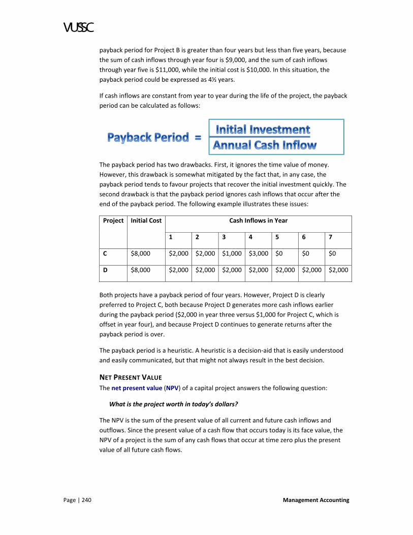
Page | 240 Management Accounting
payback period for Project B is greater than four years but less than five years, because
the sum of cash inflows through year four is $9,000, and the sum of cash inflows
through year five is $11,000, while the initial cost is $10,000. In this situation, the
payback period could be expressed as 4½ years.
If cash inflows are constant from year to year during the life of the project, the payback
period can be calculated as follows:
The payback period has two drawbacks. First, it ignores the time value of money.
However, this drawback is somewhat mitigated by the fact that, in any case, the
payback period tends to favour projects that recover the initial investment quickly. The
second drawback is that the payback period ignores cash inflows that occur after the
end of the payback period. The following example illustrates these issues:
Project Initial Cost Cash Inflows in Year
1 2 3 4 5 6 7
C $8,000 $2,000 $2,000 $1,000 $3,000 $0 $0 $0
D $8,000 $2,000 $2,000 $2,000 $2,000 $2,000 $2,000 $2,000
Both projects have a payback period of four years. However, Project D is clearly
preferred to Project C, both because Project D generates more cash inflows earlier
during the payback period ($2,000 in year three versus $1,000 for Project C, which is
offset in year four), and because Project D continues to generate returns after the
payback period is over.
The payback period is a heuristic. A heuristic is a decision‐aid that is easily understood
and easily communicated, but that might not always result in the best decision.
NET PRESENT VALUE
The net present value (NPV) of a capital project answers the following question:
What is the project worth in today’s dollars?
The NPV is the sum of the present value of all current and future cash inflows and
outflows. Since the present value of a cash flow that occurs today is its face value, the
NPV of a project is the sum of any cash flows that occur at time zero plus the present
value of all future cash flows.

Management Accounting Page | 241
In the typical scenario in which there is an initial cash outlay for the acquisition of an
asset, followed by cash inflows throughout the useful life of the asset, the NPV can be
calculated as follows:
Where k is the discount rate, n is the number of periods from time zero in which the
cash inflow occurs, and the summation is over the n periods of the life of the project. If
the cash inflows are an annuity over the life of the project, the numerator in the above
equation can be moved outside of the summation to obtain the following:
The summation now depends only on k and n:
It is exactly this term that is provided in a present value table for annuities (see Table 2
at the end of this Lesson), where k represents the discount rate in the column heading,
and n represents the number of years (the row).
__________________________________________________________________
Example: The Sunrise Bakery is considering purchasing a new oven. The oven will cost
$1,500, and the owner anticipates that the oven will increase the bakery’s future net
cash inflows by $800 per year for the next five years. What is the anticipated NPV of this
capital acquisition, if the bakery’s discount rate is 10%?
NPV = ($800 x 3.7908) – $1,500 = $3,033 – $1,500 = $1,533.
The factor 3.7908 comes from Table 2: the intersection of the column for 10% and row 5. _______________________________________________________________________
Because NPV provides an absolute measure of the return from the project, not a ratio,
it tends to favour large projects. Also, the NPV calculation implicitly assumes that free
cash flows can be reinvested at the discount rate. Despite these potential drawbacks,
net present value is usually the most reliable criterion by which to judge capital projects
on an individual basis.

Page | 242 Management Accounting
INTERNAL RATE OF RETURN
The internal rate of return (IRR) is the discount rate computed such that the net present
value of the project equals zero. Software spreadsheet applications and financial
calculators usually include a function that calculates the IRR. The following example
illustrates how the IRR was approximated prior to the widespread availability of these
electronic tools.
Example: The Sunrise Bakery is considering an expansion to its outdoor dining space
that would require an initial cash outlay of $26,000 and increase net cash inflows by
$8,000 per year for four years. The owner of the bakery does not anticipate any benefit
from this expansion after year four, because at that time she hopes to finance a major
renovation of the building that would expand the indoor dining area into the location of
the patio. What is the IRR of the proposed expansion to the current outdoor dining
space?
Setting the NPV equal to zero in the NPV equation, and solving for the present value
factor:
0 = ($8,000 x the present value factor) – $26,000
present value factor = 3.25
Looking in Row 4 of Table 2 (since the life of the annuity is four years), the closest factor
to 3.25 is 3.2397 in the column for 9%. Therefore, the IRR is approximately 9%.
Relative to NPV, the advantage of IRR is that it provides a performance measure that is
independent of the size of the project. Hence, IRR can be used to compare projects that
require significantly different initial investments.
An important drawback of IRR is that it can induce managers to reject proposed projects
that shareholders would like the company to accept. For example, if the manager is
evaluated based on the average IRR of all capital projects undertaken, and if a proposed
capital project offers an IRR that is above the company’s cost of capital, but below the
average of all capital projects undertaken thus far, the proposed project would
adversely affect the manager’s performance measure, although it would increase
economic returns to shareholders.
IRR implicitly assumes that free cash flows can be reinvested at the computed internal
rate of return. This assumption is analogous to the assumption imbedded in the NPV
calculation that free cash flows can be reinvested at the discount rate. However, in the
context of IRR, the assumption is more problematic than in the context of NPV if the IRR
is unusually high or low.
NET PRESENT VALUE AND INTERNAL RATE OF RETURN
There is an important and close relationship between NPV and IRR. The NPV is greater
than zero if and only if the IRR is greater than the discount rate. This relationship
implies that if a single proposed capital investment is considered in isolation, both NPV

Management Accounting Page | 243
and IRR will provide the same answer to the question of whether or not the investment
should be undertaken.
However, NPV and IRR need not provide the same answer if projects that require
different investments are compared. Consider the following example, comparing two
projects each with a one‐year life. Assume a 10% discount rate in the NPV calculation. In
this simple setting with a one‐year life, the IRR is easily calculated as the profit divided
by the initial investment.
Project Initial
Investment
Payout at
end of
year
Net Present Value Internal Rate
of Return
A $1,000 $1,200 $91 [(1,200 ÷ 1.1) – 1,000] 20%
B $100 $200 $82 [(200 ÷ 1.1) – 100] 100%
Hence, NPV favours Project A, while IRR favours Project B. What is the “correct”
answer? The answer depends on the opportunity cost associated with the additional
$900 required to finance Project A compared with financing Project B. For example, if
the company has $1,000 to invest and can replicate Project B ten times, doing so would
clearly be preferable to Project A. On the other hand, if the company can earn only 1%
on the $900 additional funds available if Project B is chosen over Project A, then the
company prefers Project A, calculated as follows:
Project NPV IRR
A $91, as determined above 20%, as determined above
B plus $900 invested
at 1%
$8 [($1,109 ÷ 1.1) –
$1,000]
($1,109 $1,000) ÷ $1,000 = 1.1%
The $1,109 in the bottom row is the total payout at the end of the year from this
option, calculated as $200 from Project B plus $909 from the $900 investment that
earns 1%. The NPV of $8 is actually less than the NPV from Project B alone, because the
NPV of the $900 invested at 1% is negative.
In conclusion, NPV and IRR need not rank projects equivalently, if the projects differ in
size.
THE DISCOUNT RATE
The discount rate is critical in determining whether the NPV of a project is positive or
negative (and equivalently, whether the project IRR is greater or less than the discount
rate). However, the choice of discount rate is seldom obvious.
In most situations, the appropriate discount rate is the company’s cost of capital. The
cost of capital is a weighted average of the company’s cost of debt and its cost of

Page | 244 Management Accounting
equity. Interest rates on borrowings provide information about the cost of debt.
Determining the cost of equity is more difficult, and constitutes an important topic in
the area of finance. The Weighted Average Cost of Capital (WACC) is a concept from
corporate finance that frequently serves as an appropriate discount rate for capital
budgeting decisions. In some cases, however, the company would benefit from
distinguishing between the existing average cost of capital, and the marginal cost of
capital, because the cost of debt generally increases as companies become more highly
leveraged.
Many companies establish a company‐wide hurdle rate, to communicate to managers
the appropriate discount rate for investment decisions. Often, the hurdle rate seems to
exceed the company’s cost of capital, which encourages managers to act conservatively
in their capital budgeting decisions: an outcome that is difficult to justify with finance
theory.
Another option for the discount rate is the opportunity cost associated with the funds
required for the capital project. In most cases, the cost of capital and the opportunity
cost should be approximately equal. However, most of us pay a higher rate to borrow
funds than we earn on our financial investments. Hence, if a decision‐maker has cash to
either invest in a capital project or invest in the financial markets, an appropriate
discount rate for the capital project is the opportunity cost of the earnings the decision‐
maker would have earned in the financial markets. This rate is probably lower than the
cost of raising additional financing for the project.
ACCOUNTING RATE OF RETURN
The accounting rate of return (ARR) is sometimes called the book rate of return. Of the
four capital project performance measures discussed in this Lesson, the accounting rate
of return is the only performance measure that depends on the company’s accounting
choices. It is calculated as follows:
In the simple setting in which the capital project consists of the purchase of a single
depreciable asset, the numerator is the average incremental annual cash inflow
(additional revenues or the reduction in operating expenses) attributable to the asset,
minus the annual depreciation expense. The denominator is the net book investment in
the asset, averaged over the life of the asset.
________________________________________________________________________
Example: A machine costs $12,000 and increases cash inflows by $4,000 annually for
four years. The machine has zero salvage value.
Depreciation expense = $12,000 ÷ 4 = $3,000 per year.
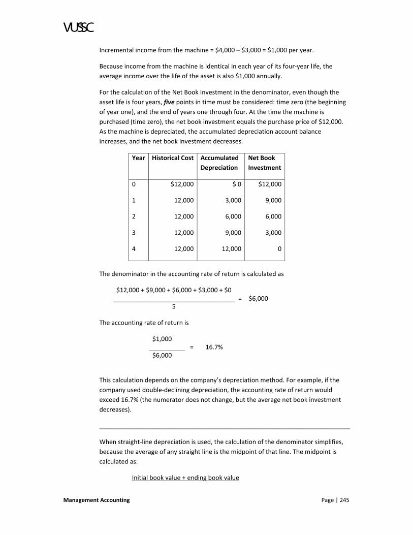
Management Accounting Page | 245
Incremental income from the machine = $4,000 – $3,000 = $1,000 per year.
Because income from the machine is identical in each year of its four‐year life, the
average income over the life of the asset is also $1,000 annually.
For the calculation of the Net Book Investment in the denominator, even though the
asset life is four years, five points in time must be considered: time zero (the beginning
of year one), and the end of years one through four. At the time the machine is
purchased (time zero), the net book investment equals the purchase price of $12,000.
As the machine is depreciated, the accumulated depreciation account balance
increases, and the net book investment decreases.
Year Historical Cost Accumulated
Depreciation
Net Book
Investment
0
1
2
3
4
$12,000
12,000
12,000
12,000
12,000
$ 0
3,000
6,000
9,000
12,000
$12,000
9,000
6,000
3,000
0
The denominator in the accounting rate of return is calculated as
$12,000 + $9,000 + $6,000 + $3,000 + $0 =
$6,000
5
The accounting rate of return is
$1,000 = 16.7%
$6,000
This calculation depends on the company’s depreciation method. For example, if the
company used double‐declining depreciation, the accounting rate of return would
exceed 16.7% (the numerator does not change, but the average net book investment
decreases).
________________________________________________________________________
When straight‐line depreciation is used, the calculation of the denominator simplifies,
because the average of any straight line is the midpoint of that line. The midpoint is
calculated as:
Initial book value + ending book value

Page | 246 Management Accounting
2
For the numerical example above, the calculation is:
$12,000 + $0 = $6,000
2
Graphically, this is illustrated as follows:
If the machine has a salvage value, and if the company accounts for that salvage value
by decreasing the depreciable basis of the asset, the salvage value has a
counterintuitive effect on the denominator of the ARR calculation: it actually increases
the company’s net book investment.
For example, assume that the machine in the example above has a salvage value of
$4,000. In this case, the annual depreciation expense is ($12,000 – $4,000) ÷ 4 = $2,000.
The schedule of net book investment is as follows:
Year Historical
Cost
Accumulated
Depreciation
Net Book
Investment
0
1
2
3
4
$12,000
12,000
12,000
12,000
12,000
$ 0
2,000
4,000
6,000
8,000
$12,000
10,000
8,000
6,000
4,000

Management Accounting Page | 247
The denominator in the accounting rate of return is then calculated as:
$12,000 + $10,000 + $8,000 + $6,000 + $4,000= $8,000
5
The accounting rate of return is then:
$4,000 $2,000 = 25%
$8,000
Again, because straight‐line depreciation is used, the denominator can be calculated
more simply as:
Initial book value + ending book value
2
which is now:
$12,000 + $4,000 = $8,000
2
and graphically:
To illustrate how the accounting rate of return depends on the company’s choice of
accounting policies, assume that instead of treating the salvage value as a reduction in
the depreciable basis of the asset, the company treats the salvage value as income in

Page | 248 Management Accounting
the year of disposal. In this case, the average annual income from the asset is calculated
as follows:
$1,000 + $1,000 + $1,000 + $5,000 = $2,000
4 years
The average net book investment is $6,000, as in the original example. The accounting
rate of return is now:
$2,000 = 33.3%
$6,000
Hence, depending on how the company chooses to treat the salvage value of the
machine, the accounting rate of return is either 25% or 33.3%.
The accounting rate of return can also be calculated year by year, instead of averaging
over the life of the project. In this case, the ARR provides information about the impact
of the project on the company’s (or division’s) return on investment, which is an
important performance measure discussed in Lesson 22.
DEPRECIATION EXPENSE, INCOME TAXES, AND CAPITAL BUDGETING
Because net present value and internal rate of return focus on cash flows, and
depreciation expense is not a cash flow, depreciation does not enter NPV and IRR
calculations directly. However, if income taxes are incorporated into the capital
budgeting decision (as should normally be the case), then depreciation expense
becomes relevant, because depreciation expense reduces taxable income, and hence,
reduces tax expense. Obviously, the capital budgeting analysis should incorporate
depreciation expense as determined for tax reporting purposes, not for financial
reporting purposes, if there is a book‐tax difference.
The reduction in taxes generated by depreciation expense is sometimes called the
depreciation tax shield.
The effect of income taxes can also be incorporated into the payback period and the
accounting rate of return in a straightforward manner. In other words, any of these
capital budgeting techniques can be applied on a pre‐tax or a post‐tax basis.

Management Accounting Page | 249
PRESENT VALUE TABLES
Table 1: Present value of $1 received (or paid) n years from now
n 6% 7% 8% 9% 10% 11% 12% 13% 14% 15% 20%
1
2
3
4
5
6
7
8
9
10
11
12
13
14
15
16
17
18
19
20
0.9434
0.8900
0.8396
0.7921
0.7473
0.7050
0.6651
0.6274
0.5919
0.5584
0.5268
0.4970
0.4688
0.4423
0.4173
0.3936
0.3714
0.3503
0.3305
0.3118
0.9346
0.8734
0.8163
0.7629
0.7130
0.6663
0.6227
0.5820
0.5439
0.5083
0.4751
0.4440
0.4150
0.3878
0.3624
0.3387
0.3166
0.2959
0.2765
0.2584
0.9259
0.8573
0.7938
0.7350
0.6806
0.6302
0.5835
0.5403
0.5002
0.4632
0.4289
0.3971
0.3677
0.3405
0.3152
0.2919
0.2703
0.2502
0.2317
0.2145
0.9174
0.8417
0.7722
0.7084
0.6499
0.5963
0.5470
0.5019
0.4604
0.4224
0.3875
0.3555
0.3262
0.2992
0.2745
0.2519
0.2311
0.2120
0.1945
0.1784
0.9091
0.8264
0.7513
0.6830
0.6209
0.5645
0.5132
0.4665
0.4241
0.3855
0.3505
0.3186
0.2897
0.2633
0.2394
0.2176
0.1978
0.1799
0.1635
0.1486
0.9009
0.8116
0.7312
0.6587
0.5935
0.5346
0.4817
0.4339
0.3909
0.3522
0.3173
0.2858
0.2575
0.2320
0.2090
0.1883
0.1696
0.1528
0.1377
0.1240
0.8929
0.7972
0.7118
0.6355
0.5674
0.5066
0.4523
0.4039
0.3606
0.3220
0.2875
0.2567
0.2292
0.2046
0.1827
0.1631
0.1456
0.1300
0.1161
0.1037
0.8850
0.7831
0.6931
0.6133
0.5428
0.4803
0.4251
0.3762
0.3329
0.2946
0.2607
0.2307
0.2042
0.1807
0.1599
0.1415
0.1252
0.1108
0.0981
0.0868
0.8772
0.7695
0.6750
0.5921
0.5194
0.4556
0.3996
0.3506
0.3075
0.2697
0.2366
0.2076
0.1821
0.1597
0.1401
0.1229
0.1078
0.0946
0.0829
0.0728
0.8696
0.7561
0.6575
0.5718
0.4972
0.4323
0.3759
0.3269
0.2843
0.2472
0.2149
0.1869
0.1625
0.1413
0.1229
0.1069
0.0929
0.0808
0.0703
0.0611
0.8333
0.6944
0.5787
0.4823
0.4019
0.3349
0.2791
0.2326
0.1938
0.1615
0.1346
0.1122
0.0935
0.0779
0.0649
0.0541
0.0451
0.0376
0.0313
0.0261
Table 2: Present value of an annuity of $1 received (or paid) each year for the next n years
n 6% 7% 8% 9% 10% 11% 12% 13% 14% 15% 20%
1
2
3
4
0.9434
1.8334
2.6730
3.4651
0.9346
1.8080
2.6243
3.3872
0.9259
1.7833
2.5771
3.3121
0.9174
1.7591
2.5313
3.2397
0.9091
1.7355
2.4869
3.1699
0.9009
1.7125
2.4437
3.1024
0.8929
1.6901
2.4018
3.0373
0.8850
1.6681
2.3612
2.9745
0.8772
1.6467
2.3216
2.9137
0.8696
1.6257
2.2832
2.8550
0.8333
1.5278
2.1065
2.5887

Page | 250 Management Accounting
Table 2: Present value of an annuity of $1 received (or paid) each year for the next n years
n 6% 7% 8% 9% 10% 11% 12% 13% 14% 15% 20%
5
6
7
8
9
10
11
12
13
14
15
16
17
18
19
20
4.2124
4.9173
5.5824
6.2098
6.8017
7.3601
7.8869
8.3838
8.8527
9.2950
9.7122
10.1059
10.4773
10.8276
11.1581
11.4699
4.1002
4.7665
5.3893
5.9713
6.5152
7.0236
7.4987
7.9427
8.3577
8.7455
9.1079
9.4466
9.7632
10.0591
10.3356
10.5940
3.9927
4.6229
5.2064
5.7466
6.2469
6.7101
7.1390
7.5361
7.9038
8.2442
8.5595
8.8514
9.1216
9.3719
9.6036
9.8181
3.8897
4.4859
5.0330
5.5348
5.9952
6.4177
6.8052
7.1607
7.4869
7.7862
8.0607
8.3126
8.5436
8.7556
8.9501
9.1285
3.7908
4.3553
4.8684
5.3349
5.7590
6.1446
6.4951
6.8137
7.1034
7.3667
7.6061
7.8237
8.0216
8.2014
8.3649
8.5136
3.6959
4.2305
4.7122
5.1461
5.5370
5.8892
6.2065
6.4924
6.7499
6.9819
7.1909
7.3792
7.5488
7.7016
7.8393
7.9633
3.6048
4.1114
4.5638
4.9676
5.3282
5.6502
5.9377
6.1944
6.4235
6.6282
6.8109
6.9740
7.1196
7.2497
7.3658
7.4694
3.5172
3.9975
4.4226
4.7988
5.1317
5.4262
5.6869
5.9176
6.1218
6.3025
6.4624
6.6039
6.7291
6.8399
6.9380
7.0248
3.4331
3.8887
4.2883
4.6389
4.9464
5.2161
5.4527
5.6603
5.8424
6.0021
6.1422
6.2651
6.3729
6.4674
6.5504
6.6231
3.3522
3.7845
4.1604
4.4873
4.7716
5.0188
5.2337
5.4206
5.5831
5.7245
5.8474
5.9542
6.0472
6.1280
6.1982
6.2593
2.9906
3.3255
3.6046
3.8372
4.0310
4.1925
4.3271
4.4392
4.5327
4.6106
4.6755
4.7296
4.7746
4.8122
4.8435
4.8696
LESSON PROBLEMS
Problem 1
Part A ‐ A project requires an initial cash outlay of $800, and returns $1,000 at the end
of year 3 (nothing at the end of years 1 or 2).
a. What is the approximately Net Present Value of this project, using a cost of
capital of 10%?
Part B ‐ A project requires an initial cash outlay of $5,000, and returns $1,000 at the end
of each year from Year 1 through Year 10.
b. What is the project’s approximate Internal Rate of Return.
Part C ‐ Refer to the project in part (B).
c. What is the Payback Period of the Project?

Management Accounting Page | 251
d. Also, what is the Accounting Rate of Return on the average net investment,
assuming that the $5,000 purchase price is for a machine that is depreciated
using straight‐line depreciation over 10 years, with zero salvage value?
Problem 2
A machine costs $4,000 (paid out at the beginning of year 1), and generates year‐end
net cash inflows of $2,000 per year for five years (this is the useful life of the machine).
The machine has zero salvage value. The company uses straight‐line depreciation and a
10% cost of capital.
a. What is the payback period for this project?
b. What is the net present value of this project?
c. What is the accounting rate of return for this project?
Problem 3
A company purchases an asset for $40,000. The asset has a useful life of seven years.
The salvage value is expected to be $10,000.
a. For purposes of computing the accounting rate of return (i.e., the book rate of
return), what is the average net investment in the asset, if the salvage value is
used to reduce the depreciable basis of the asset?
Problem 4
a. What is the net present value of a project that requires an initial cash outlay of
$1,000, and returns $7,000 at the end of seven years, using a discount rate of
12%?
Problem 5:
An investment of $400 will yield a single, lump‐sum payoff of $1,000 after 10 years.
a. At a discount rate of 7%, what is the Net Present Value of this project?
Problem 6
A machine that costs $1,000 will save $200 in operating costs every year for the next
seven years.
a. What is the approximate Internal Rate of Return of this capital project?
Problem 7
A project requires an initial investment of $500, and will return $100 per year for 11
years.
a. Using a discount rate of 9%, what is this project’s Net Present Value?

Page | 252 Management Accounting
Problem 8
A machine costs $50,000 (paid out at the beginning of year 1), and generates year‐end
net cash inflows of $8,834 per year for 12 years (this is the useful life of the machine).
The machine has zero salvage value. The company uses straight‐line depreciation.
a. What is the internal rate of return?
b. What is the net present value, using a discount rate of 10%?
c. What is the accounting rate of return?
Problem 9
a. Using an 11% discount rate, what is the net present value of a project that
requires cash outlays of $10,000 at the beginning of years one, three and five,
and provides cash inflows of $20,000 at the end of years one, three and five?
You may assume that the present value of a cash flow at the end of year X is
equivalent to the cash flow of an equivalent amount at the beginning of year X +
1 (e.g., December 31, 2005 is the same as January 1, 2006).
Problem 10
The Seven Flags over the Land of Enchantment amusement park plans to build a new
roller coaster that will be faster, higher, scarier and more thrilling than its existing roller
coasters. Seven Flags uses a 12% discount rate to evaluate capital expenditures. The
cost to prepare the site and construct the new coaster is $550,000, and this expenditure
will be incurred evenly throughout 2007 and 2008 (which is equivalent to a single cash
outlay of $550,000 incurred on December 31, 2007). The new coaster will be finished at
the beginning of 2009. The operating costs for the new coaster will be $30,000 per year
beginning January 1, 2009 (assume that the annual operating cost is incurred at the
beginning of each year). The additional revenue due to additional ticket sales are
projected to be $200,000 per year for eight years (the projected life of the coaster) from
the time the coaster opens at the beginning of 2009 through 2016 (assume, for
simplicity, that the annual revenue is received at the end of each year). At the end of
2016, the amusement park will pay $150,000 to remove the coaster.
a. Calculate the net present value of the new roller coaster, as of January 1, 2007.
Problem 11
Consider a capital project with a one‐year life. The cash outlay for the equipment occurs
at the beginning of year one, and a single cash in‐flow occurs at the end of year one.
The equipment has zero salvage value. Straight‐line depreciation is used. Indicate which
of the following statements are true.
a. If the payback period is less than one, the net present value will be greater than
zero.
b. The internal rate of return is half of the accounting (book) rate of return.
c. The inverse of the payback period equals the internal rate of return plus one.

Management Accounting Page | 253
d. The payback period is the inverse of the internal rate of return.
e. If the internal rate of return is greater than the discount rate, the net present
value will be greater than zero.
Problem 12
Consider the following two possible capital projects:
Project Initial Cost
(incurred at
beginning of
year 1)
Project
Life
Salvage
Value
Positive annual
cash flow
(received at the
end of each year)
A $200,000 16 years $0 $28,000
B $56,000 14 years $0 $9,783
Using the above information, it can be shown that the Internal Rate of Return of Project
B is higher than the Internal Rate of Return of project A.
a. Is the NPV for Project A higher than, equal to, or lower than, the NPV for Project
B, assuming a 10% discount rate?
b. Is the Payback Period for Project A better than, equal to, or worse than, the
Payback Period for Project B?
c. Is the Accounting Rate of Return for Project A higher than, equal to, or lower
than, the Accounting Rate of Return for Project B, assuming straight‐line
depreciation?
d. If the discount rate is 11% instead of 10%, which project has the higher NPV?
e. If the discount rate is 10%, and both projects have a salvage value of $66,000
(i.e., the equipment for Project B actually appreciates), which project would
have the higher NPV?
Problem 13
A machine with a useful life of five years and a salvage value of $4,000 is purchased for
$20,000. The benefit of the machine is that it reduces normal cash operating expenses
by $5,000 per year during the first two years of the machine’s life, and by $4,000 for
each of the following three years.
a. Calculate the accounting rate of return for the project, assuming that the full
$20,000 purchase price is depreciated using the straight‐line method, so that at
the end of year five, the machine has a book value of zero, and the salvage value
is treated as income in year five.
b. Calculate the accounting rate of return for the project, assuming that the net
cost of the machine (purchase price less salvage value) is depreciated using the
straight‐line method.

Page | 254 Management Accounting
Problem 14
Plain Vanilla Industries purchases a machine for $120,000. The machine has a six year
life and a salvage value of zero. The company depreciates the machine using the sum‐
of‐the‐years‐digits method, which results in depreciation expense in each year as
follows:
Year 1
Year 2
Year 3
Year 4
Year 5
Year 6
$34,286
28,571
22,857
17,143
11,429
5,714
$120,000
The machine increases cash inflows to the firm by $30,000 in year one, $35,000 in year
two, $40,000 in year three, $35,000 in year four, and $25,000 in year five.
a. Calculate the accounting rate of return from the investment in the machine.
Problem 15
A machine can be purchased for $120,000 that increases cash flows by $20,000 each
year for the next six years. In addition, the machine has a salvage value of $20,000,
which is used to reduce the depreciable basis of the asset. Assume the purchase price is
paid at the beginning of the first year, and that all cash inflows are received at the end
of each year. The company uses sum‐of‐the‐years‐digits depreciation, which results in
the following depreciation schedule:
Year 1
Year 2
Year 3
Year 4
Year 5
Year 6
$28,571
23,810
19,048
14,286
9,524
4,761
a. Compute the Accounting Rate of Return.

Management Accounting Page | 255
Problem 16
A company is considering purchasing a machine that will reduce its operating costs. The
purchase requires a down payment of $5,000, and three equal annual payments of
$3,000, due at the beginning of the second, third and fourth years of the life of the
machine. The machine will reduce operating expenses in an amount equivalent to
$2,000 received at the end of each year for eight years. The machine has a useful life of
eight years, at the end of which it has a salvage value of $1,500. The company records
the purchase of the machine at $14,000 (i.e., interest expense is not imputed), and
treats the salvage value as a reduction in the depreciable basis of the asset. The asset is
depreciated using straight‐line depreciation. The discount rate is 8%.
a. Calculate the payback period, the net present value, and the average accounting
rate of return.
LESSON SUMMARY
In this lesson we examined the creation and management of capital budgets. Capital
budgets are different from operating budgets in that the financial impact of the budget
is spread out over several years and thus must be accounted for in a different way. The
purchase of assets needed to operate the business are often part of the capital
budgeting process. As they get older their value will depreciate and your capital
budgets must reflect their depreciated value. In the next lesson will look at the creation
and management of annual operating budgets.

Page | 256 Management Accounting
LESSON 5.2: OPERATING BUDGETS
LESSON INTRODUCTION
An operating budget is business projection of your expenses and revenues over a
specific period of time. Specifically it is a detailed projection of all estimated income
and expenses based on forecasted sales revenue during a given period (usually one
year). It generally consists of several sub‐budgets, the most important one being the
sales budget, which is prepared first. Since an operating budget is a short‐term budget,
the capital outlays are excluded because they are multi‐year long‐term costs. They are
reflected in a capital budget. This lesson will explore the concepts supporting the
creation of operating budgets.
Lesson Objectives
Upon completion of this lesson you will be able to:
1. Explain the use and create:
a. a sales budget,
b. production budget,
c. accounts receivable budget,
d. accounts payable budget, and
e. cash budget.
2. Read and analyse a pro forma income statement.
3. Read and analyse a pro forma balance sheet.
OVERVIEW
A budget is a quantitative plan for the future that assists the organization in
coordinating activities. Many organizations prepare detailed budgets that look one year
ahead, and budgets that look further into the future that contain relatively less detail
and more general strategic direction.
The budget assists in the following activities:
Planning. A budget helps identify the resources that are needed, and when they
will be needed.
Control. A budget helps control costs by setting spending guidelines.
Motivating Employees. A budget can motivate employees and managers.
Budgets are more effective motivational tools if employees and managers “buy
into” the budget, which is more likely to occur if they participate in the
preparation of the budget in a meaningful way.
Communication. A budget can provide either one‐way (top‐down) or two‐way
communication within the organization.
A company’s overall budget, which is sometimes called a master budget, consists of
many supporting budgets. These supporting budgets include:
Sales budget.
Management Accounting Page | 257
Pro forma income statement.
The production budget and supporting schedules.
Budgets for capital assets and for financing activities.
Budgets for individual balance sheet accounts and departmental expenses.
Cash budget, including cash disbursements and cash receipts budgets.
Pro forma balance sheet.
There is a logical sequence for the preparation of these budgets. The first step in a
corporate setting is almost always to forecast sales and to assemble a sales budget.
THE SALES BUDGET
The individuals who are best able to forecast sales are usually the sales force and
product managers. Their ability to accurately forecast sales depends on the nature of
the industry and on characteristics of the product. Demand is seasonal for many
products, in which case each month’s forecast usually incorporates information about
sales for the same month last year. Accurately forecasting sales of new products and
fashion products can be difficult. Demand for some products is sensitive to
macroeconomic forces such as interest rates and foreign exchange rates. On the other
hand, given the seemingly arbitrary way in which most of us decide where to eat lunch,
restaurants can usually predict each day’s lunch revenue with astounding accuracy.
Most companies face a downward‐sloping demand curve for their products, which
implies that forecasting sales revenue requires predicting sales volume at the planned
sales price.
PRO FORMA INCOME STATEMENT
With planned sales prices, forecasted sales volumes, and an understanding of the cost
structure of the business, the company can assemble a pro forma income statement (an
anticipated income statement for the upcoming period). This process is illustrated
below, in a simple one‐product setting, for the Guess Who Jeans Company. The planned
sales price is $40 per unit. Assume that the sales manager’s best guess of sales volume
at this price is 20,000 units for October. Then anticipated revenue for October is
$800,000. The company’s cost structure is characterized by $30 of variable
manufacturing costs per unit, and $150,000 in fixed manufacturing and S.G.&A. (selling,
general and administrative) costs. This information is sufficient to complete the pro
forma income statement that is shown below.

Page | 258 Management Accounting
GUESS WHO JEANS PRO FORMA CONTRIBUTION MARGIN INCOME STATEMENT FOR OCTOBER
Income Statement Account
Budgeted amount Per unit
Sale of 20,000 units
Revenue
Variable manufacturing costs:
Materials
Labour
Overhead
Total
Contribution margin
Fixed costs:
Manufacturing overhead
Selling, general & admin.
Total fixed costs
Operating income
$40
15
10
5
30
$10
$800,000
300,000
200,000
100,000
600,000
200,000
100,000
50,000
150,000
$50,000
THE PRODUCTION BUDGET
The next step in the budgeting process is more complicated for manufacturing firms
than for merchandising firms, because manufacturing companies have three types of
inventory accounts: raw materials, work‐in‐process and finished goods. However,
regardless of the number of asset accounts involved, the goal is to determine the
required additions to each account (purchases or transfers‐in from an upstream
account). The calculation to determine required additions is derived by expanding the
Sources = Uses equality as follows:
Beginning balance + additions = transfers out + ending balance
This calculation sometimes uses physical quantities, and sometimes uses dollar values,
depending on which makes the most sense under the circumstances.
The beginning balance equals the ending balance for the prior period, which is available
either from actual results (the ending balance sheet), or from another budget if the
start of the period being budgeted is in the future.

Management Accounting Page | 259
The ending balance is a target established by the company, and is usually based on
anticipated activity for the following period (that is, the period following the one for
which the current budget is being prepared).
Transfers‐out equals the demand for the asset derived from a previous step in the
budgeting process:
If the asset account is finished goods inventory, the demand is based on cost of
goods sold, as derived from the pro forma income statement.
If the asset account is work‐in‐process inventory, the demand is based on the
additions to the finished goods account, as calculated by applying the sources =
uses equation shown above to the finished goods account.
If the asset account is raw materials inventory, the demand is based on the
additions to the work‐in‐process account for materials, as calculated by applying
the sources = uses equation shown above to the work‐in‐process account.
The unknown in the sources = uses equation is additions, which can be solved for, thus
completing the production budget. The following table provides balance sheet
information for Guess Who Jeans for September 30, which is the period just ended.
(This is also the beginning balance for October 1, the period for which the budget is
being prepared, because balance sheet amounts at the end of the day on September 30
are the same as the opening balances on the morning of October 1). We will use the
information in this table to budget for October’s production. Because Guess Who Jeans
makes only one product, it is more convenient to use physical quantities in the sources
= uses equations than dollars. We assume that the budget for October is being prepared
on October 1st.
GUESS WHO JEANS BALANCE SHEET
SEPTEMBER 30 (THE MONTH JUST ENDED)
Assets Amount Liabilities Amount
Cash
Accounts Receivable
Inventory:
Raw Materials (1,800 yards)
Work in Process (1,500 units)
Finished Goods (5,000 units)
Total inventory
Property, Plant & Equipment,
net of accumulated depreciation
$ 67,000
676,000
13,500
35,000
150,000
198,500
880,000
Accounts Payable
Line of Credit
Stockholders’ Equity:
Common stock
Additional paid‐in capital
Retained earnings
Total S/H equity
$ 295,000
345,000
100,000
72,500
1,009,000
1,181,500

Page | 260 Management Accounting
Assets Amount Liabilities Amount
Total $1,821,500 Total $1,821,500
Required additions to finished goods inventory: Guess Who Jeans expects to sell
20,000 units each month for the next two months (October and November). The
company would like to have on hand, at the beginning of each month, 20% of next
month’s sales. The company did not achieve this operational goal for October, because
5,000 units are on hand on October 1, and expected sales are 20,000 units, but the
company came close to its goal (25% versus 20%). At the end of October, the company
would like to have 4,000 units on hand (20% of 20,000 units expected to be sold in
November).
Beginning balance + additions = transfers out + ending balance
5,000 units + additions = 20,000 units in expected sales + 4,000 units for desired
ending inventory
additions = 19,000
Hence, Guess Who Jeans should plan to transfer out 19,000 units from work‐in‐process
to finished goods inventory during the month of October.
Required additions to work‐in‐process: Guess Who Jeans would like to have on hand,
at any point in time, 1,200 units in work‐in‐process. The company has determined that
this level of work‐in‐process provides optimal efficiency on the production line. (As
shown above, the level of work‐in‐process is slightly higher than desired at the end of
September.)
Beginning balance + additions = transfers out + ending balance
1,500 units + additions = 19,000 units transferred to finished goods + 1,200 units for
desired ending WIP
additions = 18,700
Hence, Guess Who Jeans should plan to start production of 18,700 units during the
upcoming month of October.
Required additions to raw materials: On average, 2 yards of fabric are required for
each unit of product. Guess Who Jeans would like to maintain 2,000 yards of fabric on
hand at any point in time. (The company had less fabric on hand than desired at the end
of September.)
Beginning balance + additions = transfers out + ending inventory
1,800 yards + additions = (2 yards per unit x 18,700 units) + 2,000 yards desired in
ending inventory on October 31

Management Accounting Page | 261
1,800 yards + additions = 37,400 yards + 2,000 yards
Additions = 37,600 yards of fabric
Hence, Guess Who Jeans should plan to purchase 37,600 yards of fabric during the
month of October. Using the budgeted cost of $7.50 per yard, the expected expenditure
for these fabric purchases is $282,000.
ACCOUNTS RECEIVABLE AND ACCOUNTS PAYABLE BUDGETS
Accounts Receivable: To budget for the ending balance of accounts receivable, the
company incorporates information about the rate at which receivables are collected.
Guess Who Jeans makes all sales on credit, and past experience indicates that the
following collection schedule can be anticipated:
50% of sales are collected in the month of sale
30% of sales are collected in the month following the sale
20% of sales are collected two months following the sale
This collection schedule implies that on October 31, accounts receivable will consist of:
50% of October sales
20% of September sales
Nothing from sales that occurred prior to September
(E.g., August sales would be collected in August, September, and October)
Actual sales for September were 25,000 units.
Anticipated sales for October are 20,000 units.
Therefore, the budget for accounts receivable at the end of October can be calculated
as follows:
50% of October sales
20% of September sales
20,000 units x $40 per unit x 50% = $400,000
25,000 units x $40 per unit x 20% = 200,000
$600,000
However, this calculation does not incorporate information available about September
collections of September sales and September collections of prior month sales. Possibly,
September collections of September sales differed from the 50% that is budgeted, or
perhaps not all of August’s sales were collected by the end of September. This
additional information would normally be used to refine the budget of Accounts
Receivable at the end of October.
Accounts Payable: To budget for the ending balance of accounts payable, the company
incorporates information about the extent to which the company makes purchases on

Page | 262 Management Accounting
credit. Guess Who Jeans pays cash for all types of purchases except for fabric purchases.
The company pays for fabric 30 days after the fabric is purchased, on average.
This payment policy implies that at the end of October, accounts payable will consist of
all October purchases of fabric, and nothing else. In the raw materials budget (see
above), we determined that $282,000 would be incurred for fabric purchases in
October. Hence, this amount is the anticipated the balance in Accounts Payable on
October 31.
THE CASH BUDGET
One of the most important components of the budgeting process for most
organizations is the cash budget. The cash budget indicates how much cash the
company will have on hand at the end of each period, and also indicates when the
company will need to borrow funds to cover temporary cash shortfalls, and when the
company will have excess funds to invest in short‐term financial instruments. Cash flow
is so important that in some organizations, cash balances are projected for the end of
each week, or even on a daily basis.
Often, the cash budget is assembled from supporting schedules. These schedules show,
for the period being budgeted, anticipated cash disbursements and cash receipts that
arise from (1) operating activities, (2) additions and disposals of fixed assets, and (3)
financing activities.
Cash Receipts: the company anticipates that the only cash receipts that will occur in
October will come from collections of receivables. Cash receipts in October are based
on anticipated collections of sales that were made in August and September, and
anticipated sales for October, and are projected as follows:
Sales made
in the
month of:
Sales volume
during the
month
Unit
sales
price
percentage
collected
during
October
Collections
in October
August
September
October
22,000
25,000
20,000
$40
$40
$40
20%
30%
50%
$176,000
300,000
400,000
$876,000

Management Accounting Page | 263
Cash disbursements are anticipated as follows:
Fabric purchases (for fabric acquired in September)
Manufacturing labour
Manufacturing variable overhead
Fixed manufacturing overhead (excluding non‐cash items)
Fixed selling, general and admin. overhead (excluding non‐cash items)
Cash payments for capital acquisitions (from the capital budget)
Payments of short‐term borrowings
Total disbursements for October
$295,000
189,000
94,500
50,000
35,000
110,000
60,000
$833,500
This information about receipts and disbursements is used to project the ending cash
balance for the month, as follows:
Beginning balance + cash receipts cash disbursements = ending balance
$67,000 + $876,000 $833,500 = $109,500
PRO FORMA BALANCE SHEET
The foregoing analysis can be used to assemble a pro forma balance sheet, projecting
the balance sheet at the end of the October. The amounts in the pro forma balance
sheet are derived as follows:
Cash: from the cash budget, shown above.
Accounts receivable: from the accounts receivable budget, shown above.
Raw materials inventory: from the projected ending inventory of 2,000 yards
multiplied by the budgeted price of $7.50 per yard.
Work‐in‐process inventory:
Beginning balance
+ Fabric additions (37,400 yards x $7.50 per yard)
+ Manufacturing labour (from the cash disbursements budget)
+ Manufacturing variable overhead (from the cash disbursements budget)
Transfers out to finished goods inventory (19,000 units x $30 per unit)
Ending balance
$ 35,000
280,500
189,000
94,500
570,000
$ 29,000

Page | 264 Management Accounting
Finished goods inventory: from the projected ending inventory of 4,000 units,
multiplied by the budgeted cost of $30 per unit. (Note: the company uses Variable
Costing for internal reporting.)
Property, plant & equipment, net of accumulated depreciation:
Beginning balance
+ Capital acquisitions (from the cash disbursements budget)
Depreciation expense
Ending balance
$880,000
110,000
65,000
$925,000
The $65,000 in depreciation expense reconciles to the non‐cash portion of the $150,000
in fixed manufacturing and fixed selling, general and administrative costs shown on the
pro forma income statement. The difference of $85,000 (i.e., the cash portion of these
fixed costs) is shown on the cash disbursements budget as $50,000 for fixed
manufacturing overhead and $35,000 for fixed selling, general and administrative
overhead.
Accounts payable: from the accounts payable budget, shown above.
Short‐term borrowings: beginning balance of $345,000 less the anticipated payment of
$60,000 as per the cash disbursements budget.
Common stock and Additional paid‐in capital: no change.
Retained earnings: beginning balance of $1,009,000 + October income of $50,000, as
per the pro forma income statement.
GUESS WHO JEANS PRO FORMA BALANCE SHEET
OCTOBER 31
Assets Amount Liabilities Amount
Cash
Accounts Receivable
Inventory:
Raw Materials (2,000 yards)
Work in Process (1,200 units)
Finished Goods (4,000 units)
Total inventory
$109,500
600,000
15,000
29,000
120,000
164,000
Accounts Payable
Line of Credit
Stockholders’ Equity:
Common stock
Additional paid‐in capital
Retained earnings
Total S/H equity
$282,000
285,000
100,000
72,500
1,059,000
1,231,500
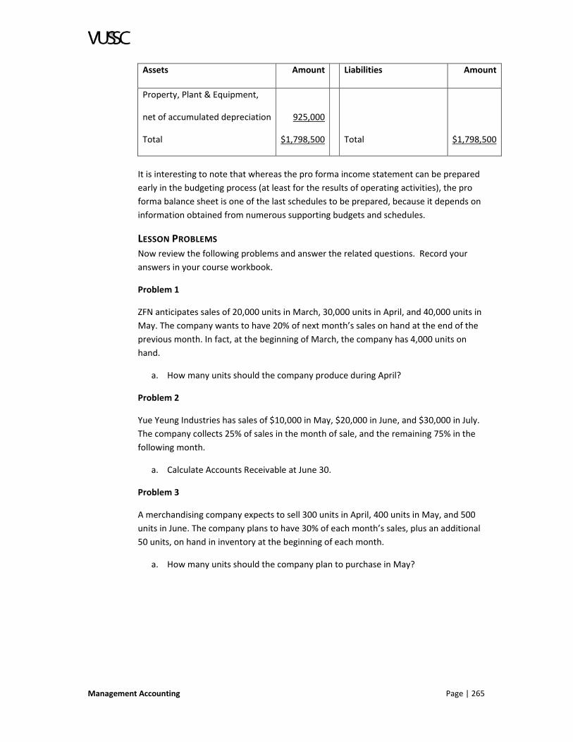
Management Accounting Page | 265
Assets Amount Liabilities Amount
Property, Plant & Equipment,
net of accumulated depreciation
Total
925,000
$1,798,500
Total $1,798,500
It is interesting to note that whereas the pro forma income statement can be prepared
early in the budgeting process (at least for the results of operating activities), the pro
forma balance sheet is one of the last schedules to be prepared, because it depends on
information obtained from numerous supporting budgets and schedules.
LESSON PROBLEMS
Now review the following problems and answer the related questions. Record your
answers in your course workbook.
Problem 1
ZFN anticipates sales of 20,000 units in March, 30,000 units in April, and 40,000 units in
May. The company wants to have 20% of next month’s sales on hand at the end of the
previous month. In fact, at the beginning of March, the company has 4,000 units on
hand.
a. How many units should the company produce during April?
Problem 2
Yue Yeung Industries has sales of $10,000 in May, $20,000 in June, and $30,000 in July.
The company collects 25% of sales in the month of sale, and the remaining 75% in the
following month.
a. Calculate Accounts Receivable at June 30.
Problem 3
A merchandising company expects to sell 300 units in April, 400 units in May, and 500
units in June. The company plans to have 30% of each month’s sales, plus an additional
50 units, on hand in inventory at the beginning of each month.
a. How many units should the company plan to purchase in May?

Page | 266 Management Accounting
Problem 4
Quolala is a merchandising company. Quolala expects unit sales for the coming year as
follows:
March 15,000
April 23,000
May 31,000
June 47,000
July 56,000
The average selling price is $23 per unit. The company’s policy is to maintain month‐end
inventory levels at 30% of next month’s anticipated sales. All sales are made on credit,
and expected collections are as follows:
70% collected in the month of sale
20% collected in the month following the sale
10% collected in the second month following the sale.
Cost of goods sold equals 80% of the sales price. The company pays cash for all
purchases of inventory, at the time of purchase.
b. How much inventory (how many units) will Quolala expect to purchase in June?
c. What will be the dollar amount of accounts receivable at the end of July?
d. How much should the company expect to pay (i.e., credits to cash, debits to
inventory) for purchases of inventory in May?
e. What can the company expect to collect in receivables (i.e., debits to cash,
credits to accounts receivable) in June?
Problem 5
The Gordon Candy Company is a wholesaler for peanut brittle and other candies.
Gordon’s sales of peanut brittle for the last four months of 2006 are projected as
follows:
September 150 cases
October 170 cases
November 190 cases
December 230 cases
Bill Gordon, founder, Chairman, President, and Chief Executive Officer of the company,
plans to sell each case for $150, which represents a 25% mark‐up over cost (Note: an
item purchased for $1 and sold for $1.60 would represent a 60% mark‐up over cost).

Management Accounting Page | 267
Bill manages his inventory purchases so that he has 45% of each month’s sales on hand
at the beginning of the month. Bill makes all purchases on credit. Bill pays 60% of credit
purchases in the month of purchase, and pays the remaining 40% in the month
following the purchase.
On average, Bill’s customers pay cash at the time of purchase for 50% of purchases, and
buy the remaining 50% on credit. Credit purchases are paid to the Gordon Candy
Company as follows:
40% in the month of purchase
35% in the month immediately following the purchase
20% in the second month following the purchase
5% bad debt expense (Bill never collects this amount).
a. Calculate the cash inflows from sales of peanut brittle and the cash outflows
from purchases of peanut brittle, for November.
Problem 6
California Concepts sells hair products. Sales of shampoo for the last half of 2005 are
projected as follows:
September: 100 cases
October: 120 cases
November: 130 cases
December: 160 cases
California Concepts plans to sell each case for $25, which represents a $7 mark‐up over
cost. The company manages its inventory purchases so that it always has 70% of each
month’s unit sales on hand at the beginning of that month. The company buys
inventory on credit. The company pays for these credit purchases in the month
following the purchase.
On average, the company’s customers pay cash at the time of purchase for 60% of their
purchases, and buy the remaining 40% on credit. These credit purchases are paid to
California Concepts as follows:
30% in the month of purchase
40% in the month immediately following the purchase
30% in the second month following the purchase
a. Calculate Accounts Receivable for sales of shampoo as of the end of November,
and Accounts Payable for purchases of shampoo as of the end of November.
b. Calculate net cash flows from sales and purchases of shampoo that occur in
November.
Page | 268 Management Accounting
Problem 7
The Piombino Manufacturing Company anticipates sales as follows:
September
October
November
December
40,000 units
45,000 units
55,000 units
62,000 units
Piombino plans to have 35% of each month’s sales on hand as finished goods inventory
at the beginning of the month. The manufacturing process requires 30 days (one
month) from start to finish. Each unit requires two pounds of aluminium, and the
aluminium is put into the production process at the beginning of production (day one of
the 30 day production cycle). Aluminium costs $15 per pound. The company wants to
have 50,000 pounds of aluminium raw materials on hand at the beginning of each
month. Purchases of aluminium are paid 50% in the first month after purchase and 50%
in the second month after purchase.
a. How much money will be disbursed in November for aluminium?
Problem 8
Mary River Distributors sells brandy and other alcoholic beverages. Sales of brandy for
the last four months of 2005 are projected as follows:
September 1,700 cases
October 1,900 cases
November 2,300 cases
December 2,800 cases
The increase through the year arises due to the increasing popularity of brandy as the
weather turns cold, and particularly the high consumption around the holiday season.
Mary River plans to sell each case for $250, which represents a 35% mark‐up over cost
(Note: an item purchased for $1 and sold for $1.60 would represent a 60% mark‐up).
Mary River manages its inventory purchases so that it always has 40% of each month’s
sales on hand at the beginning of the month. The company buys all brandy on credit.
The company pays 60% of credit purchases in the month of purchase, and pays the
remaining 40% in the month following the purchase.
On average, Mary River’s customers pay cash at the time of purchase for 20% of their
purchases, and buy the remaining 80% on credit. These credit purchases are paid to
Mary River as follows:

Management Accounting Page | 269
50% in the month of purchase
25% in the month immediately following the purchase
20% in the second month following the purchase
5% bad debt expense (Mary River never collects this amount).
a. Because “cash is king,” Mary River asks you to calculate the net cash inflows
(receipts less disbursements) from sales and purchases of brandy, in November.
Problem 9: Muravera, Inc., budgets sales as follows:
April
May
June
July
August
September
October
$520,000
600,000
580,000
450,000
420,000
470,000
500,000
Sales are 30% cash sales and 70% credit sales. Credit sales are collected, on average,
according to the following schedule:
In the month of purchase
In the first month after purchase
In the second month after purchase
In the third month after purchase
In the fourth month after purchase
Total
25%
30%
20%
15%
10%
100%
a. If all goes according to the budget, what will be the balance in Accounts
Receivable at September 30?
Problem 10
The Dorsely Manufacturing Company anticipates sales of 62,000 units in April, 55,000
units in May, 45,000 units in June, 38,000 units in July, and 29,000 units in August.
Dorsely plans to have 40% of each month’s sales on hand as finished goods inventory at
the beginning of the month. The manufacturing process requires 60 days (two months)
from start to finish. Each unit requires three feet of wire, and the wire is put into the

Page | 270 Management Accounting
production process half‐way through production (day 30 of the 60‐day production
cycle). Wire costs $7 per foot. The company wants to have 110% of each month’s wire
raw materials requirements on hand at the beginning of the month. Purchases of wire
are paid 50% in the month of purchase and 50% in the first month after purchase.
a. What will be the balance for Accounts Payable for wire at June 30?
Problem 11
Edwin’s Clothing Store expects revenues of $27,000 in March, $32,000 in April, $33,000
in May, and $36,000 in June. Eighty percent of these revenues are cash sales, and the
remaining 20% are credit sales. Bad debt expense is accrued monthly such that the
allowance for uncollectible accounts (the contra‐asset balance sheet account) is 10% of
the gross receivables at the end of any given month. Credit sales are collected as
follows: 10% in the month of sale, 35% in the month following the sale, 25% in the
second month following the sale, and 20% in the third month following the sale. Ten
percent is never collected, and uncollected accounts receivable are written off at the
end of the third month following the sale.
a. Calculate net accounts receivable (net of the allowance for uncollectible
accounts) as of June 30 (after the closing entries for the month have been
made).
Problem 12
The Trinidad Community Hospital expects patient revenues of $240,000 in March,
$250,000 in April, $270,000 in May, and $260,000 in June. Anticipated collections are as
follows: 40% of patient revenues are from Medicare patients, and Medicare reimburses
the hospital in the month after the services are provided (i.e. payment is received the
month after the revenue has been recognized). 10% of the revenues are from Medicaid
patients, and Medicaid reimburses the hospital two months after the services are
provided. 30% of the revenues are from patients covered by private insurance, and the
insurance companies reimburse the hospital 50% in the month of service, and 50% in
the month following service. 20% of the patients are not covered by insurance at all.
Among these patients, there is a bad debt rate of 30%. Bad debt expense is accrued in
the month the revenue is earned. The revenue that is collected from these patients is
received as follows: 10% in the month of service, 30% in the month following service,
40% in the second month following service, and 20% in the third month following
service.
a. Calculate patient receivables at June 30, net of the allowance for uncollectible
accounts.
LESSON SUMMARY
This lesson discussed how to plan and control annual operating budgets. Operating
budgets include a number of different cost factors which may be reflected as sub‐
budgets of the business (e.g. Sales, Production, Cash, etc.). Operating budgets also
Management Accounting Page | 271
reflect the company’s projected and actual income, as well as expenses. The data
reflected in the annual operating budget is sorted and analysed using a number of
different reports including: income statements and balance sheets. The ability to
monitor and control annual operating budgets is essential to the success of any
business.
In the next lesson we will explore some incentives that managers can offer to ensure
that budgets are effectively managed.

Page | 272 Management Accounting
LESSON 5.3: BUDGETARY INCENTIVE SCHEMES
LESSON INTRODUCTION
As discussed in the last lesson, most budgets are built on sales forecasts, and hence,
budgets are only as accurate as those forecasts. The sales force has the most accurate
and complete information about future sales prospects. Therefore, sales personnel are
the best source for the sales forecast, and one would expect the budgeting process to
begin with input from the sales force.
Furthermore, the success of most companies depends in large part on the ability of the
sales force to generate sales. In order to motivate sales personnel to work hard, many
companies include sales commissions as an important component of sales personnel’
compensation packages: the more they sell, the more they earn.
We will explore budgetary incentive schemes in this lesson.
LESSON OBJECTIVES
Upon completion of this lesson you will be able to explain different incentive schemes.
SALES INCENTIVES
For many companies, and in many industries, a straight commission is not viewed as
equitable. Some sales representatives have “easier” sales territories or product lines. A
fixed percentage commission applied to all members of the sales force seems unfair to
sales representatives who are assigned more difficult product lines or territories. Many
companies solve this problem by paying sales representatives a bonus based on actual
sales relative to budgeted sales. The budget can be tailored for each sales
representative, so that the difficulty of meeting and exceeding budget is comparable for
all sales personnel. Such a bonus scheme rewards sales representatives for incremental
effort and sales volume, relative to some baseline.
Taken together, the preceding explanation creates an obvious dilemma. The company
relies on the sales force to accurately forecast sales for budgeting purposes, yet sales
representatives, when asked for their forecasts, will budget conservatively. In so doing,
they give themselves easy targets that help ensure that they will maximize their
bonuses.
One possible solution to this dilemma is to not pay bonuses based on actual
performance relative to budget. An alternative solution is to not ask the sales
representatives for their forecasts, but simply to assign targeted sales goals. Neither
solution is optimal, because the first solution limits the company’s ability to motivate
the sales force using a bonus scheme that is generally perceived as effective and fair,
and the second solution ignores information that would materially assist in the
budgeting process.
One might wonder whether a better solution is possible. In fact, budgetary incentive
schemes that simultaneously address these two apparently conflicting objectives have
been used for at least 25 years. The example described in the rest of this Lesson is
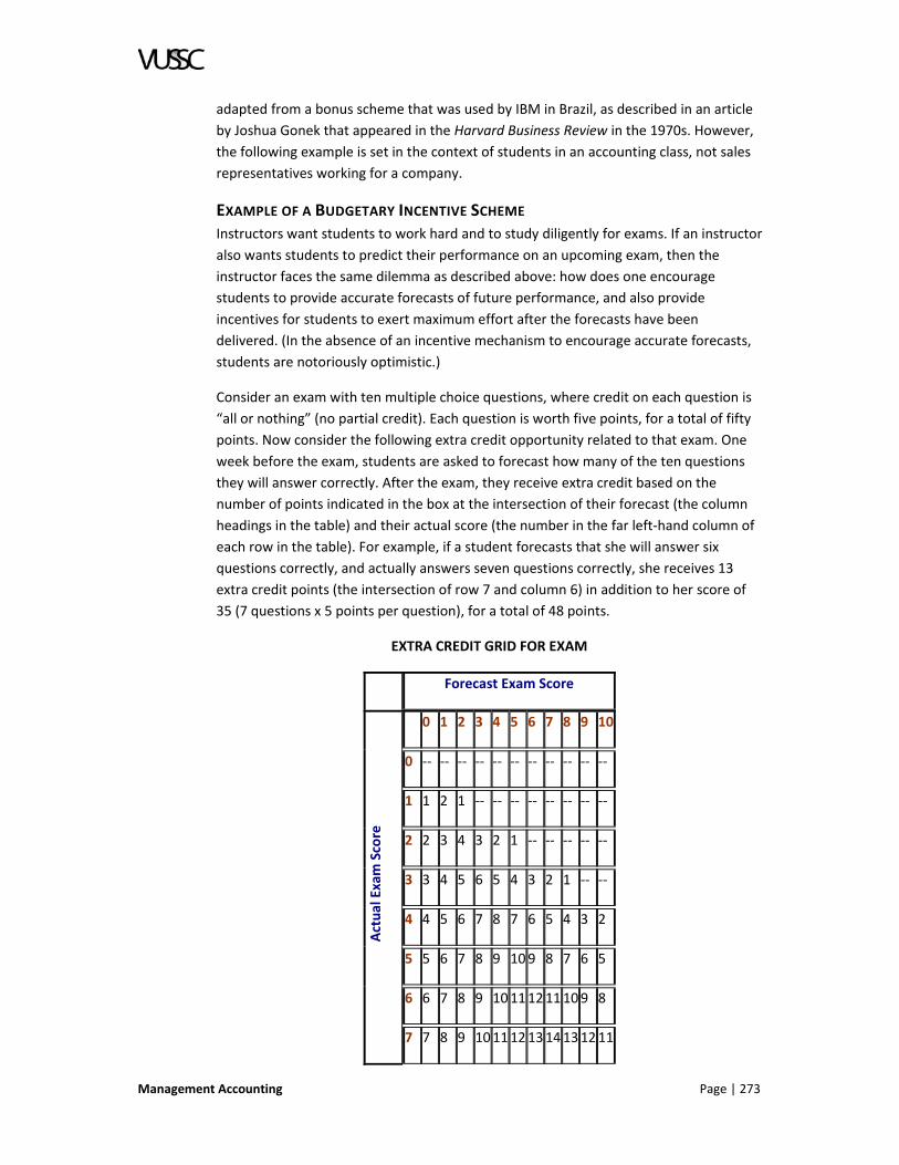
Management Accounting Page | 273
adapted from a bonus scheme that was used by IBM in Brazil, as described in an article
by Joshua Gonek that appeared in the Harvard Business Review in the 1970s. However,
the following example is set in the context of students in an accounting class, not sales
representatives working for a company.
EXAMPLE OF A BUDGETARY INCENTIVE SCHEME
Instructors want students to work hard and to study diligently for exams. If an instructor
also wants students to predict their performance on an upcoming exam, then the
instructor faces the same dilemma as described above: how does one encourage
students to provide accurate forecasts of future performance, and also provide
incentives for students to exert maximum effort after the forecasts have been
delivered. (In the absence of an incentive mechanism to encourage accurate forecasts,
students are notoriously optimistic.)
Consider an exam with ten multiple choice questions, where credit on each question is
“all or nothing” (no partial credit). Each question is worth five points, for a total of fifty
points. Now consider the following extra credit opportunity related to that exam. One
week before the exam, students are asked to forecast how many of the ten questions
they will answer correctly. After the exam, they receive extra credit based on the
number of points indicated in the box at the intersection of their forecast (the column
headings in the table) and their actual score (the number in the far left‐hand column of
each row in the table). For example, if a student forecasts that she will answer six
questions correctly, and actually answers seven questions correctly, she receives 13
extra credit points (the intersection of row 7 and column 6) in addition to her score of
35 (7 questions x 5 points per question), for a total of 48 points.
EXTRA CREDIT GRID FOR EXAM
Forecast Exam Score
Actual Exam Score
0 1 2 3 4 5 6 7 8 9 10
0 ‐‐ ‐‐ ‐‐ ‐‐ ‐‐ ‐‐ ‐‐ ‐‐ ‐‐ ‐‐ ‐‐
1 1 2 1 ‐‐ ‐‐ ‐‐ ‐‐ ‐‐ ‐‐ ‐‐ ‐‐
2 2 3 4 3 2 1 ‐‐ ‐‐ ‐‐ ‐‐ ‐‐
3 3 4 5 6 5 4 3 2 1 ‐‐ ‐‐
4 4 5 6 7 8 7 6 5 4 3 2
5 5 6 7 8 9 109 8 7 6 5
6 6 7 8 9 10111211109 8
7 7 8 9 1011121314131211

Page | 274 Management Accounting
Forecast Exam Score
8 8 9 101112131415161514
9 9 10111213141516171817
101011121314151617181920
This scheme encourages students to forecast accurately, and once the students have
made their forecasts, to study hard for the exam. To see that the extra credit scheme
achieves both objectives, note the following:
When the student makes her forecast, she is choosing the column that will be used to
determine her extra credit. Within each column, the numbers become larger as one
moves down the table. Therefore, once the forecast has been delivered, students want
to score as high as possible to maximize both the extra credit score and the total exam
score.
Now consider the question of whether students have incentives to forecast accurately.
At the time that the student makes her forecast, she has an idea of what her actual
score will be. Hence, she has a best‐guess of the row that will be used to determine her
extra credit. In any given row, the maximum bonus occurs in the column for which the
row heading equals the column heading. For example, if the student thinks she will
answer five questions correctly, then her maximum extra credit from row “5” is ten,
which occurs in the column labelled “5.” Therefore, if she thinks she will score five, she
cannot expect to do better than to forecast five, the same as her expected
performance. If she intentionally forecasts low (choosing a column to the left of column
5) or forecasts high (choosing a column to the right of column 5), she can anticipate
earning less than ten extra credit points if she actually answers five questions correctly,
as she predicts.
This extra credit scheme is an example of a budgetary incentive scheme that
encourages individuals to both forecast accurately, and to exert maximum effort after
the forecast has been delivered. Implicit in this scheme, and all such schemes, is a
“baseline” performance level. For example, in the extra credit scheme, if the instructor
anticipates that the median on the exam will be six, then it is important that students
have approximately the same expectation. If the exam turns out to be more difficult or
easier than anticipated, then students’ forecasts will be “high” or “low” on average, and
the amount of extra credit earned will be less than otherwise would have been the
case. The extra credit scheme would still encourage accurate forecasts and maximum
effort, but it probably would not be perceived as “fair” after the scores are in. Hence,
this specific scheme and all such schemes rely on some level of accuracy in
management’s (or the instructor’s) information, but then uses that information to
obtain still more accurate information from the individuals who are best informed (sales
representatives or students, as the case may be).

Management Accounting Page | 275
LESSON PROBLEMS
Now review the following problems and answer the related questions. Record your
answers in your course workbook.
Problem 1: The table below represents a bonus scheme, in which the sales
representative is given a quota (called the objective), is asked to provide a forecast for
her sales volume for the upcoming year, and then is given a bonus (expressed as a
percentage of a baseline bonus) based on a combination of her forecast and actual
results. The numbers in the grid represent the percentage of the baseline bonus that
the sales representative will receive. For example, if the sales representative is given a
quota of 300 units and she forecasts that she can sell 600 units, F/O = 2.0, and she will
be working from the column with 2.0 in the heading. Then, if she sells 450 units, her
bonus will be calculated from the number at the intersection of the column labelled 2.0
and the row labelled 1.5 (A/O = 450/300 = 1.5). The number in that box is 120, so she
will receive 120% of the baseline bonus.
F/O = forecast ÷ objective
A/O
= Actual ÷ Objective
0 0.5 1.0 1.5 2.0 2.5 3.0 3.5 4.0 4.5 5.0
0 ‐‐ ‐‐ ‐‐ ‐‐ ‐‐ ‐‐ ‐‐ ‐‐ ‐‐ ‐‐ ‐‐
0.5 60 30 ‐‐ ‐‐ ‐‐ ‐‐ ‐‐ ‐‐ ‐‐ ‐‐ ‐‐
1.0 90 120 90 60 30 ‐‐ ‐‐ ‐‐ ‐‐ ‐‐ ‐‐
1.5 120 150 180 150 120 90 60 30 ‐‐ ‐‐ ‐‐
2.0 150 180 210 240 210 180 150 120 90 60 30
2.5 180 210 240 270 300 270 240 210 180 150 120
3.0 210 240 270 300 330 360 330 300 270 240 210
3.5 240 270 300 330 360 390 420 390 360 330 300
4.0 270 300 330 360 390 420 450 480 450 420 390
4.5 300 330 360 390 420 450 480 510 540 510 480
5.0 330 360 390 420 450 480 510 540 570 600 570
a. Evaluate this bonus scheme, and discuss in two or three sentences how effective
the incentives imbedded in this bonus scheme are likely to be, in terms of
motivating the sales representative to provide her best forecast of her sales
volume for the upcoming year, and to work hard to achieve and even exceed her
forecasted sales volume, once her forecast has been made.

Page | 276 Management Accounting
Problem 2: The table below represents a bonus scheme, in which the sales
representative is given a quota (called the objective), is asked to provide a forecast for
her sales volume for the upcoming year, and then is given a bonus (expressed as a
percentage of a baseline bonus) based on a combination of her forecast and actual
results. The numbers in the grid represent the percentage of the baseline bonus that
the sales representative will receive. For example, if the sales representative is given a
quota of 300 units and she forecasts that she can sell 600 units, F/O = 2.0, and she will
be working from the column with 2.0 in the heading. Then, if she sells 450 units, her
bonus will be calculated from the number at the intersection of the column labelled 2.0
and the row labelled 1.5 (A/O = 450/300 = 1.5). The number in that box is 180, so she
will receive 180% of the baseline bonus.
F/O = forecast ÷ objective
A/O
= Actual ÷ Objective
0 0.5 1.0 1.5 2.0 2.5 3.0 3.5 4.0 4.5 5.0
0 ‐‐ ‐‐ ‐‐ ‐‐ ‐‐ ‐‐ ‐‐ ‐‐ ‐‐ ‐‐ ‐‐
0.5 ‐‐ 30 60 30 ‐‐ ‐‐ ‐‐ ‐‐ ‐‐ ‐‐ ‐‐
1.0 30 60 90 120 90 60 30 ‐‐ ‐‐ ‐‐ ‐‐
1.5 60 90 120 150 180 150 120 90 60 30 ‐‐
2.0 90 120 150 180 210 240 210 180 150 120 90
2.5 120 150 180 210 240 270 300 270 240 210 180
3.0 150 180 210 240 270 300 330 360 330 300 270
3.5 180 210 240 270 300 330 360 390 420 390 360
4.0 210 240 270 300 330 360 390 420 450 480 450
4.5 240 270 300 330 360 390 420 450 480 510 540
5.0 270 300 330 360 390 420 450 480 510 540 570
a. Evaluate this bonus scheme, and discuss in two to four sentences how effective
the incentives imbedded in this bonus scheme are likely to be, in terms of
motivating the sales representative to provide her best forecast of her sales
volume for the upcoming year, and to work hard to achieve and even exceed her
forecasted sales volume, once her forecast has been made.
LESSON SUMMARY
This lesson described different incentive schemes that can be used to motivate and
reward subordinate managers to achieve their budget estimates. The next lesson will
explore how to measure the successful performance of your managers.

Management Accounting Page | 277
LESSON 5.4: DIVISIONAL PERFORMANCE MEASURES
LESSON INTRODUCTION
It is key to any successful business to measure the performance of its strategic
direction, business plans, financial plans and the ability of the managers to implement
and manage the plans effectively. Performance measurement is a process for
collecting and reporting information regarding the performance of an individual, group
or organizations. It can involve looking at process/strategies in place, as well as whether
outcomes are in line with what was intended or should have been achieved. This
includes all financial plans and budgets.
This lesson discusses three performance measures used to evaluate divisions and
divisional managers. The term “division” in this lesson is shorthand for any
responsibility centre that is treated as a profit centre or as an investment centre.
Investors and stock analysts use analogous measures to evaluate company‐wide
performance.
LESSON OBJECTIVES
Upon completion of this lesson you will be able to:
1. Explain divisional income.
2. Calculate Return on Investment.
3. Explain residual income
DIVISIONAL INCOME
Divisional income is a measure of divisional performance that is analogous to corporate
net income for evaluating overall company performance. Similar to related‐party
transactions in the context of financial accounting, the calculation of divisional income
must consider transactions that occur between divisions, and between the division and
corporate headquarters. One type of intra‐company transaction is the transfer of goods
between divisions. These transfers, which represent revenue to the selling division and
a cost of inventory to the buying division, are discussed in Lesson 23. Another type of
transaction is the receipt of services from corporate headquarters or from other
responsibility centres within the company. Examples of such services are human
resources, legal, risk management, and computer support. In many companies, these
services are “charged out” to the divisions that utilize them. These service department
cost allocations were discussed in Lesson 12.
Because divisional income fails to account for the size of the division, it is ill‐suited for
comparing performance across divisions of different sizes. Divisional income is most
meaningful as a performance measure when compared to the same division in prior
periods, or to budgeted income for the division.

Page | 278 Management Accounting
RETURN ON INVESTMENT
Return on investment (ROI) is calculated as:
The same issues arise in determining the numerator in ROI as arise in the previous
subsection with respect to deriving divisional income. As regards the denominator,
senior management must decide whether and how to allocate shared assets among
divisions, such as service departments at the corporate level, or shared manufacturing
facilities. Also, management must decide how to value the capital assets that comprise
the division’s investment. These assets can be valued at their gross book value (the
acquisition cost), their net book value (usually the acquisition cost minus depreciation
expense), or less often, some other valuation technique such as replacement cost, net
realizable value or fair market value. The calculation of the numerator should be
consistent with the choice of valuation technique in the denominator. For example, if
divisional investment is calculated using gross book value, then divisional income in the
numerator should not be reduced by depreciation expense.
One advantage of using gross book value instead of net book value in the ROI
calculation is that net book value can discourage divisional managers from replacing old
equipment, even if new equipment would be more efficient and would increase the
economic profits of the division. This dysfunctional managerial incentive occurs because
if the existing equipment is fully depreciated, but is still functional, its replacement can
reduce the division’s ROI by lowering the numerator (due to increased depreciation
expense) and increasing the denominator (because fully depreciated assets have a net
book value of zero).
ROI can be broken down into the following two components:
The first term on the right‐hand side is called the return on sales (ROS). It is also called
the operating profit percentage. This ratio measures the amount of each dollar of
revenue that “makes its way” to the bottom line. ROS is often an important measure of
the efficiency of the division, and the divisional manager’s ability to contain operating
expenses.
The second term on the right‐hand side is called the asset turnover ratio or the
investment turnover ratio. This ratio measures how effectively management uses the
division’s assets to generate revenues. Interestingly, this ratio seems to hover around
one for many companies in a wide range of industries, particularly in the manufacturing
sector of the economy.

Management Accounting Page | 279
Breaking ROI into these two components often provides more useful information than
looking at ROI alone, and it is an example of the type of financial ratio analysis that
stock analysts conduct in evaluating company‐wide performance. In this context, two
common specifications for the denominator in the ROI calculation are assets and equity.
The resulting ratios are called return on assets (ROA) and return on equity (ROE).
At the divisional level, ROI controls for the size of the division, and hence, it is well‐
suited for comparing divisions of different sizes. On the other hand, similar to the
Internal Rate of Return for evaluating capital projects, ROI can discourage managers
from making some investments that shareholders would favour. For example, if a
divisional manager is evaluated on ROI, and if the division is currently earning an ROI in
excess of the company’s cost of capital, then the manager would prefer to reject an
additional investment opportunity that would earn a return above the cost of capital
but below the division’s current ROI. The new investment opportunity would lower the
division’s ROI, which is not in the manager’s best interests. However, because the
investment opportunity provides a return above the cost of capital, shareholders would
favour it.
RESIDUAL INCOME
One way in which financial accounting practice fails to follow corporate finance theory
is that the cost of debt is treated as an expense in arriving at net income, but the cost of
equity is not. Specifically, interest expense appears as a deduction to income on the
income statement, but dividends are shown on the statement of changes in
shareholders’ equity. Hence, net income is affected by the company’s financing strategy
as well as by its operating profitability, which can obscure the economic performance of
the firm.
A simple solution to this problem is to add back interest expense (net of the tax effect)
to net income, to arrive at operating income after taxes. The performance measure
called residual income makes this adjustment, and then goes one step further, by
deducting a charge for capital based on the organization’s total asset base:
Residual Income = Operating Income (Investment Base x Required Rate of Return)
The company’s cost of capital is often appropriate for the required rate of return.
Residual income is probably the closest proxy that accounting provides for the concept
of economic profits; hence, residual income probably comes close to measuring what
shareholders really care about (to the extent that shareholders only care about
maximizing wealth). Residual income can be calculated both at the corporate level and
at the divisional level. Many companies that use residual income at the divisional level
do so because management believes that residual income aligns incentives of divisional
managers with incentives of senior management and shareholders.
One type of residual income calculation is called Economic Value Added. EVA was
developed by the consulting firm of Stern Stewart & Co., and is a registered trademark
of that firm. The calculation of EVA includes a deduction for the cost of capital, and also

Page | 280 Management Accounting
adjusts accounting income to more accurately reflect the economic effect of
transactions and the economic value of assets and liabilities. In general, these
adjustments move the income calculation further from the reliability‐end of the
relevance‐versus‐reliability continuum, and closer to the relevance‐end of that
continuum.
Since the 1990s, EVA has helped revive the popularity of residual income. However, it
should be emphasized that although Stern Stewart has obtained trademark protection
on the term “EVA,” the concept of residual income precedes EVA by almost half a
century, and it is in the public domain. Anyone can use residual income for any purpose
whatsoever without violating trademark, copyright or patent law, and this includes
making obvious adjustments to net income to more accurately reflect the underlying
economic reality of the firm.
LESSON PROBLEMS
Now review the following problems and answer the related questions. Record your
answers in your course workbook.
Problem 1
The Purini Dog Food Company has two divisions, the Puppy Chow Division and the
Canine Elder Division. Operating results for the two divisions are as follows:
Puppy Chow Division Canine Elder Division
Net Operating Income $10,000 $ 6,000
Average Operating Assets $50,000 $42,000
The required rate of return, which is equal to the cost of capital, is 10%.
Required: A project with a return of $20,000 on an investment of $130,000 exists. If the
divisions are evaluated based on return on investment, which division(s) would like to
accept the project? If the divisions are evaluated based on residual income, which
division(s) would like to accept the project?
Problem 2: Nummi Motors operates two divisions: the truck division and the car
division. Nummi’s hurdle rate (i.e., the cost of capital) is 10%. Following is information
about the two divisions:
Truck Division Car Division
Divisional Income $ 1 million $ 2 million
Divisional Operating Assets $12 million $10 million
a. Calculate the truck division’s residual income
b. Calculate the car division’s return on investment

Management Accounting Page | 281
Problem 3
A company has two divisions: the Eastern division and the Western division. The cost of
capital is 15%. Following is information about the two divisions:
Eastern Division Western Division
Divisional profits
Divisional investment
$ 100,000
1,000,000
$ 200,000
1,000,000
a. Calculate each division’s residual income, and residual income for the company
as a whole
b. Calculate each division’s return on investment, and return on investment for the
company as a whole.
Problem 4
In 1980, the truck division of Motown Motors had return on sales of 15% and an asset
turnover ratio of 50%. Sales were $100 million.
a. Calculate the division’s return on investment.
Problem 5
Recall that Residual Income is calculated by subtracting from NOPAT (Net operating
profit after taxes) a charge for the cost of capital. If a company has interest expense and
income tax expense, but no other income or expense line‐items between operating
income and net income, then NOPAT simply adds back to net income the after‐tax
effect of interest expense.
Arbatax has after‐tax net income in 2007 of $34,000,000. The company has a marginal
tax rate of 35%. The company incurred interest expense in 2007 of $6,000,000 (and the
company earned no interest income). Arbatax had total assets in 2007 of $400,000,000.
The company’s cost of capital is 8%.
a. Determine the company’s Residual Income for 2007.
Problem 6
Following is selected information from the 2005 Annual Report of General Motors
(some small miscellaneous line‐items have been excluded, so that net income
calculated from these numbers differs slightly from net income as per the annual
report):

Page | 282 Management Accounting
2005 2004
Automotive and Other Operations
Revenue
COGS, SG&A and other
Financing and Insurance Business
Revenue
Expenses
Interest expense
Net income tax benefit (increases income)
Total assets
Shareholders equity
$158,221,000,000
175,395,000,000
34,383,000,000
18,372,000,000
15,768,000,000
5,878,000,000
480,530,000,000
14,597,000,000
$161,545,000,000
162,087,000,000
31,972,000,000
18,264,000,000
11,980,000,000
916,000,000
482,347,000,000
27,360,000,000
a. Calculate GM’s pre‐tax income, after‐tax income, return on investment, and
residual income for both 2005 and 2004. Combine both segments of the
company for this exercise (automotive and financing). For return on investment,
use pre‐tax income in the numerator and total assets in the denominator. For
residual income, use a 7% cost of capital, and a marginal tax rate of 30% to
adjust for the tax effect of interest expense.
Problem 7
Following is selected information from the 2005 or 2006 financial statements of four
airlines. All amounts are in 000’s.
Southwest Airlines
Alaska Airlines
Frontier Airlines
Midwest Express
Revenue
Operating income
Net interest expense
Pre‐tax income
After‐tax income
Total assets
Shareholders equity
$7,584,000
820,000
75,000
874,000
548,000
14,218,000
6,675,000
$2,416,100
10,800
18,700
124,200
2,300
3,511,900
626,900
$994,273
7,897
12,392
20,469
13,971
970,432
228,776
$522,989
65,168
142
65,026
64,886
351,344
17,256

Management Accounting Page | 283
a. Calculate ROI for each airline using net income and total assets. Break out each
airline’s ROI into return on sales and the asset turnover ratio.
Problem 8
Following is selected financial information for four companies for 2005 (all amounts are
in millions):
Apple
Computer
Pepsi
Chevron
The GAP
Revenue
Total assets
Shareholder equity
Operating income
Net income
$13,931
11,551
7,466
1,650
1,335
$32,562
31,727
14,320
6,382
4,078
$198,200
125,833
62,676
25,197
14,099
$16,023
8,821
5,425
1,745
1,113
Required: Calculate each firm’s return on investment (net income on total assets),
return on sales, asset turnover ratio, and residual income using an 8% cost of capital.
None of these firms incurred significant interest expense during the year.
Problem 9: Following is selected segment information for 2005 from the Annual Report
for Starbucks.
United
States
(000’s)
International
(000’s)
Unallocated
Corporate
(000’s)
Total
(000’s)
Revenue
Pre‐tax earnings
Identifiable assets
$5,334,460
945,926
1,633,721
$1,034,840
86,421
605,750
$ 0
235,903
1,274,594
$6,369,300
796,444
3,514,065
The total column agrees to the company’s 2005 income statement. In answering the
following questions, because Starbucks has virtually no debt, interest expense can be
ignored. Also, assume a 33% effective tax rate and a 7% cost of capital.

Page | 284 Management Accounting
a. Calculate post‐tax return on investment and post‐tax residual income for the
United States segment, the International segment, and for the company as a
whole.
b. Explain why corporate‐level residual income is less than the sum of the residual
income of the two segments. Speculate as to the types of assets and expenses
that are included as unallocated corporate. Identify the advantages and
disadvantages of failing to allocate to the operating divisions significant
corporate‐level assets and expenses.
LESSON SUMMARY
Return on Investment is important to every business. If you have no ROI then your
business will fail. You need to ensure that your company has a positive and ideally
growing ROI. Thus you must monitor your financial investments, company revenues
and company expenses.

Management Accounting Page | 285
LESSON 5.5: TRANSFER PRICING
LESSON INTRODUCTION
A transfer price is what one part of a company charges another part of the same
company for goods or services. Transactions may include the trade of supplies or
labour between departments. Transfer prices are used when individual entities of a
larger multi‐entity firm are treated and measured as separately run entities. In this
lesson we will explore the complexities of transfer pricing.
LESSON OBJECTIVES
Upon completion of this lesson you will be able to:
1. Define and provide examples of transfer pricing.
2. Explain transfer pricing options including,
a. Market‐based transfer prices,
b. Cost‐based transfer prices,
c. Negotiated transfer prices, and
d. Dual transfer pricing.
3. Describe survey of practice.
4. Identify different external reporting methods.
5. Explain the impact of transfer pricing on multinational income taxes.
6. Explain different regulatory issues.
INTRODUCTION
Ferrari: Shall we draw up the papers, or is our handshake good enough?
Rick: It’s certainly not good enough. But since I’m in a hurry, it’ll have to do.
Ferrari: Ah, to get out of Casablanca and go to America! You’re a lucky man.
Rick: Oh, by the way, my agreement with Sam’s always been that he gets 25%
of the profits. That still goes.
Ferrari: Hmmm. I happen to know that he gets 10%. But he’s worth 25%.
Rick: Don’t forget, you owe Rick’s a hundred cartons of American cigarettes.
Ferrari: I shall remember to pay it… to myself.
From Casablanca, 1942
DEFINITION AND OVERVIEW
In the excerpt from Casablanca, Rick apparently loaned Ferrari 100 cartons of cigarettes
for which he was never repaid. Now that Ferrari owns both the Blue Parrot and Rick’s
Café, he jokes about the fact that what was previously a debt that he owed to Rick, is
now a “debt” from one nightclub that he owns to another nightclub that he owns. If
Ferrari continues to transfer cartons of cigarettes between the two clubs, he might wish
to establish a “transfer price” for cigarettes, but knowing Ferrari, he won’t bother.

Page | 286 Management Accounting
We will restrict attention to transfers that involve a tangible product, and we will refer
to the two corporate entities engaged in the transfer as divisions. Hence, the transfer
price is the price that the “selling” division charges the “buying” division for the
product. Because objects that float usually flow downstream, the selling division is
called the upstream division and the buying division is called the downstream division.
Transferred product can be classified along two criteria. The first criterion is whether
there is a readily‐available external market price for the product. The second criterion is
whether the downstream division will sell the product “as is,” or whether the
transferred product becomes an input in the downstream division’s own production
process. When the transferred product becomes an input in the downstream division’s
production process, it is referred to as an intermediate product. The following table
provides examples.
An external market
price is available
No external market
price is available
The downstream
division will sell “as
is”
The West Coast Division
of a supermarket chain
transfers oranges to the
Northwest Division, for
retail sale.
A pharmaceutical company
transfers a drug that is under
patent protection, from its
manufacturing division to its
marketing division.
The downstream
division will use the
transferred product in
its own production
process
An oil company transfers
crude oil from the drilling
division to the refinery,
to be used in the
production of gasoline.
The Parts Division of an
appliance manufacturer
transfers mechanical
components to one of its
assembly divisions.
Transfer pricing serves the following purposes.
1. When product is transferred between profit centres or investment centres
within a decentralized firm, transfer prices are necessary to calculate divisional
profits, which then affect divisional performance evaluation.
2. When divisional managers have the authority to decide whether to buy or sell
internally or on the external market, the transfer price can determine whether
managers’ incentives align with the incentives of the overall company and its
owners. The objective is to achieve goal congruence, in which divisional
managers will want to transfer product when doing so maximizes consolidated
corporate profits, and at least one manager will refuse the transfer when
transferring product is not the profit‐maximizing strategy for the company.
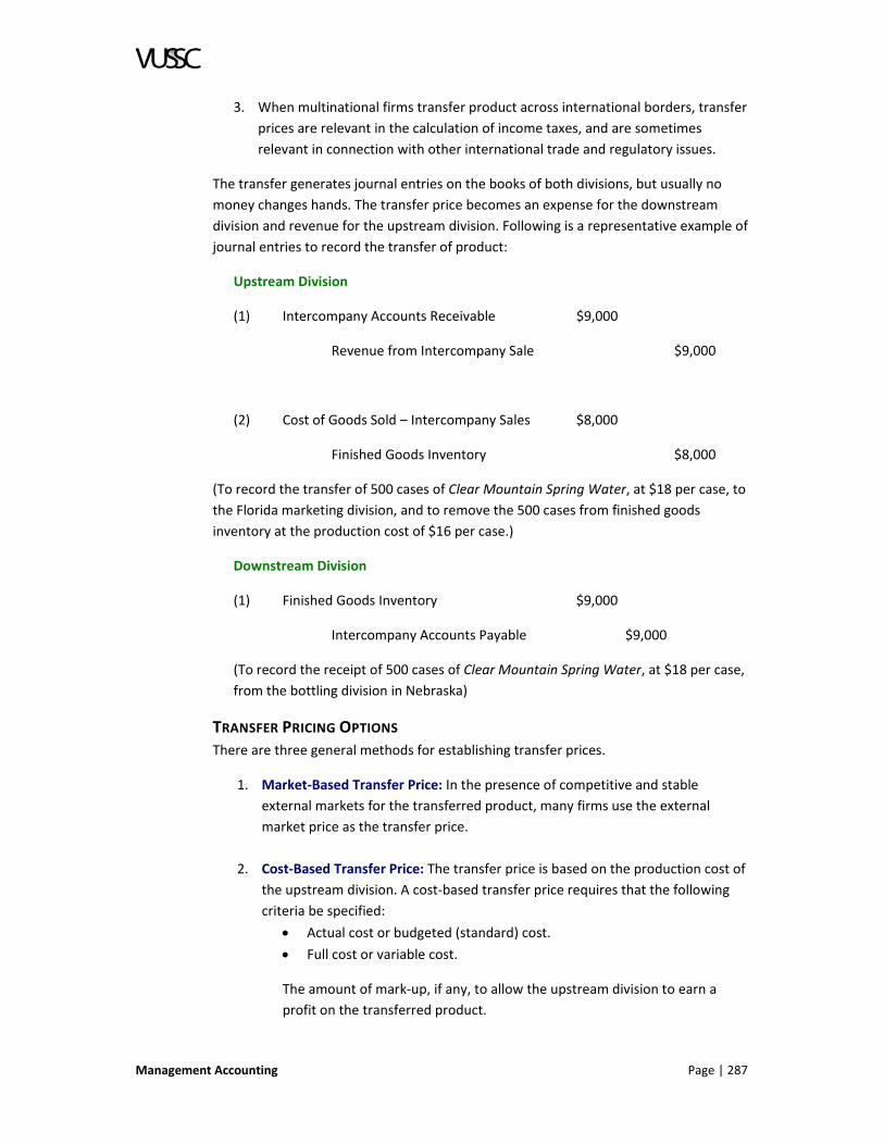
Management Accounting Page | 287
3. When multinational firms transfer product across international borders, transfer
prices are relevant in the calculation of income taxes, and are sometimes
relevant in connection with other international trade and regulatory issues.
The transfer generates journal entries on the books of both divisions, but usually no
money changes hands. The transfer price becomes an expense for the downstream
division and revenue for the upstream division. Following is a representative example of
journal entries to record the transfer of product:
Upstream Division
(1) Intercompany Accounts Receivable $9,000
Revenue from Intercompany Sale $9,000
(2) Cost of Goods Sold – Intercompany Sales $8,000
Finished Goods Inventory $8,000
(To record the transfer of 500 cases of Clear Mountain Spring Water, at $18 per case, to
the Florida marketing division, and to remove the 500 cases from finished goods
inventory at the production cost of $16 per case.)
Downstream Division
(1) Finished Goods Inventory $9,000
Intercompany Accounts Payable $9,000
(To record the receipt of 500 cases of Clear Mountain Spring Water, at $18 per case,
from the bottling division in Nebraska)
TRANSFER PRICING OPTIONS
There are three general methods for establishing transfer prices.
1. Market‐Based Transfer Price: In the presence of competitive and stable
external markets for the transferred product, many firms use the external
market price as the transfer price.
2. Cost‐Based Transfer Price: The transfer price is based on the production cost of
the upstream division. A cost‐based transfer price requires that the following
criteria be specified:
Actual cost or budgeted (standard) cost.
Full cost or variable cost.
The amount of mark‐up, if any, to allow the upstream division to earn a
profit on the transferred product.

Page | 288 Management Accounting
3. Negotiated Transfer Price: Senior management does not specify the transfer
price. Rather, divisional managers negotiate a mutually‐agreeable price.
Each of these three transfer pricing methods has advantages and disadvantages.
MARKET‐BASED TRANSFER PRICES
Microeconomic theory shows that when divisional managers strive to maximize
divisional profits, a market‐based transfer price aligns their incentives with owners’
incentives of maximizing overall corporate profits. The transfer will occur when it is in
the best interests of shareholders, and the transfer will be refused by at least one
divisional manager when shareholders would prefer for the transfer not to occur. The
upstream division is generally indifferent between receiving the market price from an
external customer and receiving the same price from an internal customer.
Consequently, the determining factor is whether the downstream division is willing to
pay the market price. If the downstream division is willing to do so, the implication is
that the downstream division can generate incremental profits for the company by
purchasing the product from the upstream division and either reselling it or using the
product in its own production process. On the other hand, if the downstream division is
unwilling to pay the market price, the implication is that corporate profits are
maximized when the upstream division sells the product on the external market, even if
this leaves the downstream division idle. Sometimes, there are cost savings on internal
transfers compared with external sales. These savings might arise, for example, because
the upstream division can avoid a customer credit check and collection efforts, and the
downstream division might avoid inspection procedures in the receiving department.
Market‐based transfer pricing continues to align managerial incentives with corporate
goals, even in the presence of these cost savings, if appropriate adjustments are made
to the transfer price (i.e., the market‐based transfer price should be reduced by these
cost savings).
However, many intermediate products do not have readily‐available market prices.
Examples are shown in the table: a pharmaceutical company with a drug under patent
protection (an effective monopoly); and an appliance company that makes component
parts in the Parts Division and transfers those parts to its assembly divisions. Obviously,
if there is no market price, a market‐based transfer price cannot be used.
A disadvantage of a market‐based transfer price is that the prices for some commodities
can fluctuate widely and quickly. Companies sometimes attempt to protect divisional
managers from these large unpredictable price changes.
COST‐BASED TRANSFER PRICES
Cost‐based transfer prices can also align managerial incentives with corporate goals, if
various factors are properly considered, including the outside market opportunities for
both divisions, and possible capacity constraints of the upstream division.
First consider the case in which the upstream division sells the intermediate product to
external customers as well as to the downstream division. In this situation, capacity
constraints are crucial. If the upstream division has excess capacity, a cost‐based

Management Accounting Page | 289
transfer price using the variable cost of production will align incentives, because the
upstream division is indifferent about the transfer, and the downstream division will
fully incorporate the company’s incremental cost of making the intermediate product in
its production and marketing decisions. However, senior management might want to
allow the upstream division to mark up the transfer price a little above variable cost, to
provide that division positive incentives to engage in the transfer.
If the upstream division has a capacity constraint, transfers to the downstream division
displace external sales. In this case, in order to align incentives, the opportunity cost of
these lost sales must be passed on to the downstream division, which is accomplished
by setting the transfer price equal to the upstream division’s external market sales
price.
Next consider the case in which there is no external market for the upstream division. If
the upstream division is to be treated as a profit centre, it must be allowed the
opportunity to recover its full cost of production plus a reasonable profit. If the
downstream division is charged the full cost of production, incentives are aligned
because the downstream division will refuse the transfer under only two circumstances:
First, if the downstream division can source the intermediate product for a lower cost
elsewhere;
Second, if the downstream division cannot generate a reasonable profit on the sale of
the final product when it pays the upstream division’s full cost of production for the
intermediate product.
If the downstream division can source the intermediate product for a lower cost
elsewhere, to the extent the upstream division’s full cost of production reflects its
future long‐run average cost, the company should consider eliminating the upstream
division. If the downstream division cannot generate a reasonable profit on the sale of
the final product when it pays the upstream division’s full cost of production for the
intermediate product, the optimal corporate decision might be to close the upstream
division and stop production and sale of the final product. However, if either the
upstream division or the downstream division manufactures and markets multiple
products, the analysis becomes more complex. Also, if the downstream division can
source the intermediate product from an external supplier for a price greater than the
upstream division’s full cost, but less than full cost plus a reasonable profit margin for
the upstream division, suboptimal decisions could result.
NEGOTIATED TRANSFER PRICES
Negotiated transfer pricing has the advantage of emulating a free market in which
divisional managers buy and sell from each other in a manner that simulates arm’s‐
length transactions. However, there is no reason to assume that the outcome of these
transfer price negotiations will serve the best interests of the company or shareholders.
The transfer price could depend on which divisional manager is the better poker player,
rather than whether the transfer results in profit‐maximizing production and sourcing
decisions. Also, if divisional managers fail to reach an agreement on price, even though
Page | 290 Management Accounting
the transfer is in the best interests of the company, senior management might decide to
impose a transfer price. However, senior management’s imposition of a transfer price
defeats the motivation for using a negotiated transfer price in the first place.
SURVEY OF PRACTICE
Roger Tang (Management Accounting, February 1992) reports 1990 survey data on
transfer pricing practices obtained from approximately 150 industrial companies in the
Fortune 500. Most of these companies operate foreign subsidiaries and also use
transfer pricing for domestic interdivisional transfers. For domestic transfers,
approximately 46% of these companies use cost‐based transfer pricing, 37% use
market‐based transfer pricing, and 17% use negotiated transfer pricing. For
international transfers, approximately 46% use market‐based transfer pricing, 41% use
cost‐based transfer pricing, and 13% use negotiated transfer pricing. Hence, market‐
based transfer pricing is more common for international transfers than for domestic
transfers. Also, comparison to an earlier survey indicates that market‐based transfer
pricing is slightly more common in 1990 than it was in 1977.
Tang also finds that among companies that use cost‐based transfer pricing for domestic
and/or international transfers, approximately 90% use some measure of full cost, and
only about 5% or 10% use some measure of variable cost.
EXTERNAL REPORTING
For external reporting under Generally Accepted Accounting Principles, no matter what
transfer price is used for calculating divisional profits, the effect should be reversed and
intercompany profits eliminated when the financial results of the divisions are
consolidated. Obviously, intercompany transfers are not arm’s‐length transactions, and
a company cannot generate profits or increase the reported cost of its inventory by
transferring product from one division to another.
DUAL TRANSFER PRICING
Under a dual transfer pricing scheme, the selling price received by the upstream division
differs from the purchase price paid by the downstream division. Usually, the
motivation for using dual transfer pricing is to allow the selling price to exceed the
purchase price, resulting in a corporate‐level subsidy that encourages the divisions to
participate in the transfer. Although dual transfer pricing is rare in practice, a thorough
understanding of dual transfer pricing illustrates some of the key bookkeeping and
financial reporting implications of all transfer pricing schemes.
In the following example, the Clear Mountain Spring Water Company changes from a
negotiated transfer price of $18 per case (see the above example) to a dual transfer
price in which the upstream division receives the local market price of $19 per case, and
the downstream division pays $17 per case.

Management Accounting Page | 291
Upstream Division:
(1) Intercompany Receivable/Payable $9,500
Revenue from Intercompany Sale $9,500
(2) Cost of Goods Sold – Intercompany Sales $8,000
Finished Goods Inventory $8,000
(To record the transfer of 500 cases of Clear Mountain Spring Water, at $19 per case, to
the Florida marketing division, and to remove the 500 cases from finished goods
inventory at the production cost of $16 per case.)
Downstream Division:
(1) Finished Goods Inventory $8,500
Intercompany Receivable/Payable $8,500
(To record the receipt of 500 cases of Clear Mountain Spring Water at $17 per case,
from the bottling division in Nebraska)
Corporate Headquarters:
(1) Interco. Receivable/Payable – Florida $8,500
Corporate Subsidy for Dual Transfer Price 1,000
Interco. Receivable/Payable – Nebraska $9,500
(To record the transfer of 500 cases of Clear Mountain Spring Water from Nebraska to
Florida, at a dual transfer price of $19/$17 per case.)
Corporate Subsidy for Dual Transfer Price is an expense account at the corporate level.
This account and the revenue account that records the intercompany sale affect the
calculation of divisional profits for internal reporting and performance evaluation, but
these accounts—as well as the intercompany receivable/payable accounts—are
eliminated upon consolidation for external financial reporting. To the extent that the
Florida Division has ending inventory, the cost of that inventory for external financial
reporting will be the company’s cost of production of $16 per case. In other words, the
transfer price has no effect on the cost of finished goods inventory.
TRANSFER PRICING AND MULTINATIONAL INCOME TAXES
When divisions transfer product across tax jurisdictions, transfer prices play a role in the
calculation of the company’s income tax liability. In this situation, the company’s
transfer pricing policy can become a tax planning tool. The United States has
agreements with most other nations that determine how multinational companies are
taxed. These agreements, which are called bilateral tax treaties, establish rules for
apportioning multinational corporate income among the nations in which the

Page | 292 Management Accounting
companies conduct business. These rules attempt to tax all multinational corporate
income once and only once (excluding the double‐taxation that occurs at the Federal
and state levels). In other words, the tax treaties attempt to avoid the double‐taxation
that would occur if two nations taxed the same income. Since transfer prices represent
revenue to the upstream division and an expense to the downstream division, the
transfer price affects the calculation of divisional profits that represent taxable income
in the nations where the divisions are based.
For example, if a U.S.‐based pharmaceutical company manufactures a drug in a factory
that it operates in Ireland and transfers the drug to the U.S. for sale, a high transfer
price increases divisional income to the Irish division of the company, and hence,
increases the company’s tax liability in Ireland. At the same time, the high transfer price
increases the cost of product to the U.S. marketing division, lowers U.S. income, and
lowers U.S. taxes. The company’s incentives with regard to the transfer price depend on
whether the marginal tax rate is higher in the U.S. or in Ireland. If the marginal tax rate
is higher in the U.S., the company prefers a high transfer price, whereas if the marginal
tax rate is higher in Ireland, the company prefers a low transfer price. The situation
reverses if the drug is manufactured in the U.S. and sold in Ireland. The general rule is
that the company wants to shift income from the high tax jurisdiction to the low tax
jurisdiction.
There are limits to the extent to which companies can shift income in this manner.
When a market price is available for the goods transferred, the taxing authorities will
usually impose the market‐based transfer price. When a market‐based transfer price is
not feasible, U.S. tax law specifies detailed and complicated rules that limit the extent
to which companies can shift income out of the United States.
OTHER REGULATORY ISSUES
Transfer pricing sometimes becomes relevant in the context of other regulatory issues,
including international trade disputes. For example, when tariffs are based on the value
of goods imported, the transfer price of goods shipped from a manufacturing division in
one country to a marketing division in another country can form the basis for the tariff.
As another example, in order to increase investment in their economies, developing
nations sometimes restrict the extent to which multinational companies can repatriate
profits. However, when product is transferred from manufacturing divisions located
elsewhere into the developing nation for sale, the local marketing division can export
funds to “pay” for the merchandise received. As a final example, when nations accuse
foreign companies of “dumping” product onto their markets, transfer pricing is often
involved. Dumping refers to selling product below cost, and it generally violates
international trade laws. Foreign companies frequently transfer product from
manufacturing divisions in their home countries to marketing affiliates elsewhere, so
that the determination of whether the company has dumped product depends on
comparing the transfer price charged to the marketing affiliate with the upstream
division’s cost of production.

Management Accounting Page | 293
LESSON PROBLEMS
Now review the following problems and answer the related questions. Record your
answers in your course workbook.
Problem 1 The McNabb Company’s Eastern Division has capacity to produce 200,000 widgets
annually. The normal selling price is $19 per widget. Fixed costs are $800,000, and
variable costs are $7 per widget. Another division of McNabb Company would like to
buy some widgets from the Eastern Division.
a. Assume the Eastern Division is operating at 100% of capacity (demand from
current customers exceeds the Eastern Division's production capacity). The
Western Division would like to purchase 10,000 widgets from the Eastern
Division, and $2 of the variable costs incurred by the Eastern Division could be
avoided on each widget transferred. What is the lowest transfer price the
Eastern Division should accept?
b. Assume that the Eastern Division is operating at 80% of capacity. The Western
Division would like to purchase 20,000 widgets. No variable cost would be
avoided on the sale. What is the lowest transfer price the Eastern Division
should accept?
c. Assume the Eastern Division is operating at 95% of capacity. The Western
Division would like to buy 40,000 widgets in an all‐or‐nothing deal (it is 40,000 or
zero). There would be no variable cost savings. What is the lowest transfer price
the Eastern Division could accept to maintain its current profitability?
Problem 2
The Upstream Division of CDC makes an intermediate product at a variable cost of $40
per unit, but the cost is $12 less per unit on internal sales, due to reduced packaging
requirements. The Division can sell everything it can produce to the outside market for
$60 per unit ($60 is the market price for the intermediate product). The Downstream
Division can use the intermediate product in its own manufacturing process. Excluding
the cost to the Downstream Division of obtaining this intermediate product, its variable
production cost is $55 per unit, and it sells its final product for $108 per unit. The
Downstream Division can buy the intermediate product from an independent supplier
for the market price of $60 per unit.
a. What is the range of transfer prices at which the managers of both divisions
would be willing to transfer product?
Problem 3
The Engineering Department of Electronics Mega‐Corporation transferred one of the
widgets that it manufactured to the Eastern Division of the company. This transfer
occurred using a transfer price of the Engineering Department’s budgeted variable cost
of production. The market price of the widget was $105.

Page | 294 Management Accounting
The Eastern Division didn’t do any work on the widget, but rather transferred the
widget to the Western Division. This transfer occurred using a transfer price of the
Engineering Department’s budgeted full cost of production.
The Western Division didn’t do any work on the widget either, but transferred the
widget to the Central Division. This transfer occurred using a transfer price of the
Engineering Department’s actual full cost of production.
The Central Division didn’t do any work on the widget either, but transferred the widget
to the Southern Division. This transfer occurred using a transfer price of the Engineering
Department’s actual full cost of production plus a 10% mark‐up.
The Southern Division didn’t do any work on the widget, but transferred the widget to
the European Division. This transfer occurred using a dual transfer price. The Southern
Division received its cost, and the European Division paid the market price.
Following is cost information for the widget and for the Engineering Department.
Budget Actual
Direct materials per unit
Direct labour hours per unit
Direct labour wage rate per hour
Variable overhead per unit
$10
1
$50
$5
$12
1
$50
$6
Fixed and variable overhead are allocated based on direct labour hours. Annual fixed
costs for the department were budgeted for $1,000,000, but actual fixed costs were
$1,200,000. Total direct labour hours for the department for the year were budgeted
for 100,000, but actual labour hours were 80,000.
a. What is the transfer price from Engineering to the Eastern Division?
b. What is the transfer price from the Eastern Division to the Western Division?
c. What is the transfer price from the Western Division to the Central Division?
d. What is the transfer price from the Central Division to the Southern Division
e. What is the transfer price paid by the European Division for the widget?
Problem 4
The Olala Juice Company makes and sells apple juice. Olala operates as two divisions:
the New York Division under the name “Yo, Juice!”; and the California Division under
the name “Wow, Juice?” Each division has a sales department and a production
department. Each production department makes the same product: organic,
wholesome, pasteurized apple juice. Usually, each division sells the juice that it makes.
However, sometimes the New York sales force sells juice to a customer on the West
Coast, in which case the most sensible thing to do is to ship the juice out of the

Management Accounting Page | 295
California division’s plant, and for purposes of calculating divisional income, transfer the
product on paper from the California Division to the New York Division. Similarly,
sometimes the California Division sells juice to an East Coast customer. Following is cost
and volume information for each division for 2004. No marketing costs are incurred on
internal sales.
New York Division California Division
(The “Yo, Juice!” Co.) (The “Wow, Juice?” Co.)
External sales 900 cases at $25 per case 1,300 cases at $25 per case
Manufacturing Costs:
Variable costs $15 per case $12 per case
Fixed costs $5,000 $13,200
Marketing Costs:
Variable Costs $1.00 per case $0.50 per case
Fixed Costs $500 $1,000
Production 1,000 cases 1,200 cases
Transfers
to the other division 200 cases 100 cases
from the other division 100 cases 200 cases
a. If transfers are made at variable manufacturing cost of the division that
produced and transfers the product, calculate the divisional income of each
division, using Variable Costing.
b. If transfers are made at full manufacturing cost of the division that produced
and transfers the product, calculate the divisional income of each division, using
Absorption Costing.
Problem 5 (Continuation of Problem 4)
Which of the following will maximize the sum of divisional operating income for the two
divisions?
a. A dual transfer price in which the selling division receives the full (variable plus
fixed) manufacturing cost and the buying division pays the market price.
b. A dual transfer price in which the selling division receives the market price and
the buying division pays the full (variable plus fixed) manufacturing cost.
c. A transfer price calculated as the variable manufacturing cost of the selling
division.

Page | 296 Management Accounting
d. Every transfer price will result in the same total for the sum of the two division’s
operating income. The transfer price only affects how this total is allocated
between the two divisions.
Problem 6 (Continuation of Problem 4)
Assume each division is producing at capacity, and that each division can sell as much
product as it produces to external customers at the market price (unlimited demand).
Each manager is allowed to decide whether to transfer product to the other division.
Which transfer price ensures that each manager is willing to transfer product to the
other division?
a. A dual transfer price in which the selling division receives the full (variable plus
fixed) manufacturing cost and the buying division pays the market price.
b. A dual transfer price in which the selling division receives the market price and
the buying division pays the full (variable plus fixed) manufacturing cost.
c. A transfer price calculated as the variable manufacturing cost of the selling
division.
d. None of the above.
Problem 7 (Continuation of Problem 4)
Assume all of the juice transferred from N.Y. to California is sold before year‐end.
However, some of the juice transferred from California to N.Y. has not been sold, and is
in ending inventory.
Which transfer pricing scheme will result in the lowest value for ending inventory for
financial reporting of the consolidated company under GAAP?
a. Variable manufacturing cost plus a 20% mark‐up.
b. Full (variable plus fixed) manufacturing cost with no mark‐up.
c. Market transfer price.
d. Each of the above transfer prices results in the same value for ending inventory.
Problem 8
Robinson Farms has two divisions, the Orchard Division, and the Kitchen Division. The
Orchard Division grows apples for a variable cost of $6 per bushel. Its 2005 sales were
150,000 bushels to outsiders at $10 per bushel and 40,000 bushels to the Kitchen
Division at 140% of variable costs. Under a dual transfer pricing system, The Kitchen
Division pays only the variable cost per bushel. The fixed manufacturing costs of the
Orchard Division were $250,000 per year.
The Kitchen Division bakes pies with the apples, and sells the pies to outside customers
for $2.00 per pie. It takes one bushel of apples to make a dozen pies. The Kitchen
Division has variable manufacturing costs of $0.40 per pie in addition to the costs from
the Orchard Division. The annual fixed manufacturing costs of the Kitchen Division were
$170,000. There were no beginning inventories or ending inventories during the year.

Management Accounting Page | 297
a. What is the operating income of the Orchard Division?
b. What is the operating income of the Kitchen Division?
c. What is the operating income of Robinson Farms as a whole?
d. Explain why the company operating income is less than the sum of the two
divisions' total income.
e. Now assume that there is no beginning or ending inventory of apples, but that
out of the 480,000 pies manufactured, Sunnybrook Kitchen has 60,000 pies
unsold at the end of 2005. Ignoring the issue of spoilage (the pies can be
frozen), how would this ending inventory be valued for financial reporting
purposes (i.e., for G.A.A.P.)? That is, what is the dollar value of this inventory on
Robinson's consolidated financial statements?
Problem 9
The Upstream Division of Consolidated Inc. makes a widget that is transferred to the
Downstream Division for further processing and eventual sale to outside customers. In
May, the Upstream Division started with zero inventory, made 1,000 widgets, and
transferred 800 widgets to the Downstream Division. The total cost to produce these
1,000 widgets was $50,000 in variable manufacturing costs and $100,000 in fixed
manufacturing costs. Since the Upstream Division is strictly a manufacturing division,
there were no non‐manufacturing costs. Although the Upstream Division did not sell
any widgets on the open market in May, there is a market for these widgets, and the
market price in May was $180 per widget. The Downstream Division processed 750 of
the 800 widgets received in May, at a total cost of $120,000 ($80,000 in variable
manufacturing costs, and $40,000 in fixed manufacturing costs), and sold 665 of these
widgets in May for $400 each. The Downstream Division incurred variable non‐
manufacturing costs of $10 per unit sold, and fixed non‐manufacturing costs of $30,000.
a. What is the market‐based transfer price? Calculate divisional income for the
Upstream Division using Absorption Costing and the market‐based transfer
price.
b. What is the transfer price if product is transferred at variable cost of
production? Calculate divisional income for the Upstream Division using
Variable Costing and a variable cost‐based transfer price.
c. What is the transfer price if the company transfers product at the full (variable
plus fixed) cost of production? Calculate divisional income for the Upstream
Division using Absorption Costing and a full cost‐based transfer price.
d. Calculate divisional income for the Downstream Division using Absorption
Costing and a market‐based transfer price.
e. Calculate divisional income for the Downstream Division using Absorption
Costing and a full cost‐based transfer price.
Problem 10
The Ohio Division of the Chocolate Company makes chocolate, sells some chocolate to
candy manufacturers, and transfers the rest of the chocolate to the Ice Cream Division
of the Chocolate Company. In January the Ohio Division made 10,000 pounds of

Page | 298 Management Accounting
chocolate, incurred variable manufacturing costs of $15,000, and fixed manufacturing
costs of $10,000. For internal reporting purposes, the company uses a full cost transfer
price (i.e., variable plus fixed manufacturing costs) for transfers of product from one
division to another. Of the 10,000 pounds of chocolate made in January, 8,000 pounds
were sold to other companies at an average sales price of $5 per pound, and 2,000
pounds were transferred to the Ice Cream Division. The Ice Cream division used 1,000
pounds of chocolate to make 10,000 gallons of chocolate ice cream. Additional costs
incurred to make the ice cream were $11,000 in variable manufacturing costs and
$20,000 in fixed manufacturing costs. All of the ice cream was sold by the end of the
month for $5 per gallon, but 1,000 pounds of the chocolate received from the Ohio
Division was still on hand at the end of January.
a. What is the transfer price for January? Calculate divisional Gross Margin using
Absorption Costing for the Ohio Division for January.
b. Calculate divisional Gross Margin using Absorption Costing for the Ice Cream
Division for January.
c. Now assume the same facts as above, except that instead of using a full cost
transfer price, the company uses a market‐based transfer price. What is the
market‐based transfer price? Calculate divisional Gross Margins for both the
Ohio Division and the Ice Cream Division using Absorption Costing and the
market‐based transfer price.
d. Assume the company uses a market‐based transfer price for internal reporting
purposes. What would the company show for external financial reporting
purposes (GAAP) at the end of January for the cost of ending inventory for the
chocolate held by the Ice Cream Division?
Problem 11
The Transylvania Salad Dressing Company operates in two countries: Rumania and
Bulgaria. The Rumanian Division has a processing facility that produces olive oil, and
also a factory that mixes and bottles salad dressing for the local market. The Bulgarian
Division has a processing facility that produces wine vinegar, and also a factory, similar
to the Rumanian factory, that mixes and bottles dressing for the local market.
Historically, the oil and vinegar processing plants have produced enough oil and vinegar
to meet the demand for both the Rumanian and Bulgarian bottling plants, and each
processing facility has sold excess product (oil or vinegar) in its local market. Following
are relevant data for 2005. All amounts have been translated into U.S. currency.
Rumanian
bottling
plant
Rumanian oil
processing
facility
Bulgarian
bottling
plant
Bulgarian
vinegar
processing
facility
Production (in gallons):
Outside sales (in gallons):
250,000
250,000
400,000
60,000
150,000
120,000
100,000
20,000

Management Accounting Page | 299
Rumanian
bottling
plant
Rumanian oil
processing
facility
Bulgarian
bottling
plant
Bulgarian
vinegar
processing
facility
Ending inventory (gallons):
Dressing
Oil
Vinegar
Variable mfg. costs:
Fixed mfg costs:
0
0
0
$0.36/gal
$100,000
0
0
0
$1.00/gal
$300,000
30,000
20,000
0
$0.22/gal
$ 30,000
0
0
0
$0.80/gal
$ 50,000
Variable costs of the bottling plants shown above do not include the costs of the vinegar
and oil, and are stated as per gallon of finished product (i.e., dressing). All outside sales
are made at the prevailing market prices in that country, as shown below.
Market Prices, per gallon:
In Bulgaria In Rumania
salad dressing: $3.00 $3.00
vinegar: $1.20 $1.40
Oil: $2.30 $2.00
Additional information: It takes 0.2 gallons vinegar and 0.8 gallons oil to make 1 gallon
of salad dressing. The company is based in Bulgaria. The company pays Rumanian taxes
on Rumanian income and Bulgarian taxes on consolidated income in excess of
Rumanian income. Rumanian income is equivalent to income of the Rumanian division
(bottling plant and oil processing plant). The tax rate for the company in Rumania is
50%, and the tax rate for the company in Bulgaria is 40%.

Page | 300 Management Accounting
a. What is the transfer price of oil using variable cost?
b. What is the transfer price of oil using full cost?
c. What is the transfer price of oil using the selling division’s market price?
d. What is the transfer price of vinegar using variable cost?
e. What is the transfer price of vinegar using full cost?
f. What is the transfer price of vinegar using the selling division’s market price
g. Assume each division buys and sells intermediate product (oil and vinegar) from
the other division. What transfer pricing policy (variable cost, full cost, or
market price of the selling division) maximizes the company’s after tax profits
for the year? The same type of transfer price (variable cost, full cost, or market
price) must be used for both vinegar and oil. You may assume that under any
transfer pricing method, taxable income in both countries will be positive.
h. Assume the company uses a market‐based transfer price for calculating its tax
expense. Compute the company’s ending inventory for financial reporting
purposes under U.S. Generally Accepted Accounting Principles.
Problem 12
The dairy in Las Placitas, New Mexico, sells milk, and makes various products from the
milk, such as cheese, powdered mild, and Milk Duds. The dairy operates as two
divisions: the Cow & Milk Division, and the Advanced Products (A.P.) Division. The
manager of the Cow & Milk Division, Beatta Bovine, can choose either to package and
sell milk directly to independent customers, or she can sell milk to the manager of the
A.P. Division. The manager of the A.P. Division can either buy milk from the Cow & Milk
Division, or buy milk on the open market, for use in the production of cheese, butter,
etc. Currently, the dairy uses a market‐based transfer price for internal sales of milk
from one division to the other. Each manager is evaluated based on meeting (or
exceeding) divisional profit targets for his or her division.
The manager of the A.P. Division, Hank Holstein, suggests changing to a full cost transfer
price with a mark‐up. The mark‐up would be computed such that if all sales of the Cow
& Milk Division were at this price, the Division would just meet its targeted profit
amount. Furthermore, Hank suggests allowing his division to buy milk on the open
market, but requiring the Cow & Milk Division to sell internally whenever the A.P.
Division wants to buy internally. Hank argues that under this new transfer pricing
scheme, his division will be no worse off than before (since if the transfer price is above
market, he can buy milk on the open market instead of internally), and that the Cow &
Milk Division should be satisfied with this transfer price, since internal sales will not pull
that Division’s profits below what would be necessary for the Division to meet its
targeted profits objective.
Under Hank’s scheme, indicate whether each of the following statements is true or
false.

Management Accounting Page | 301
a. If the market demand for milk exceeds the capacity of the Cow & Milk Division,
Beatta will never prefer to sell milk to Hank (instead of selling to the open
market) when Hank prefers to buy milk from Beatta (instead of buying on the
open market).
b. If the Cow & Milk Division has excess capacity relative to market demand,
Beatta will always want to supply milk to the Advanced Products Division.
c. This new transfer pricing scheme will ensure that the two divisions will only
transfer product when the transfer is in the best interests of the Dairy as a
whole.
d. If the Cow & Milk Division can sell all of its production to the Advanced Products
division, the new transfer pricing scheme may induce Beatta to relax cost
control pertaining to certain divisional costs.
LESSON SUMMARY
When a company is small the calculation and application of transfer pricing may not be
needed. But as a company grows and different departments take on responsibilities for
production, services, sales and marketing there will be a need to calculate transfer
pricing for goods and services provided internally and across department boundaries.
This occurs when different departments are treated as profit centres within a
decentralized company.

Page | 302 Management Accounting
LESSON 5.6: CORPORATE SOCIAL RESPONSIBILITY
“But you were always a good man of business, Jacob,” faltered Scrooge….
“Business!” cried the Ghost, wringing its hands again. “Mankind was my
business. The common welfare was my business; charity, mercy, forbearance,
and benevolence, were, all, my business. The dealings of my trade were but a
drop of water in the comprehensive ocean of my business!”
‐ Charles Dickens, A Christmas Carol
LESSON INTRODUCTION
Most of us balance multiple objectives. Probably, you are attempting to balance your
efforts across two or more classes this term, in order to earn good grades in all of them.
You are probably also balancing your accomplishments in school with other obligations
and goals related to work, hobbies, your involvement with charities, and your
relationships with friends and family. There is no “summary measure” or “overall grade”
of your success in balancing these multiple objectives and goals, all of which compete
for your time and effort.
Similarly, most government programs and organizations balance multiple objectives.
City governments allocate scarce resources across diverse activities such as public
safety, street maintenance, and public libraries. How does the citizenry choose between
two more police officers or a new children’s wing for the library? How does one develop
a single measure to evaluate the city’s overall success in meeting its goals?
Public schools have a goal not to leave any student behind. Schools also have goals to
provide challenging opportunities for the very brightest students, and to provide
extracurricular activities for all students. Schools must allocate limited resources across
these sometimes‐competing objectives.
The US National Forest Service attempts to balance the economic needs of local
communities and timber‐dependent industries with the goal of conservation and with
the goal of providing outdoor‐enthusiasts recreational opportunities on public lands.
These goals are so disparate that almost nobody thinks the Forest Service does a good
job. The National Park Service has a comparatively easier time: it only balances the two
competing objectives of conservation and recreational opportunities. Even so, the Park
Service faces controversial decisions such as closing roads to private vehicles in some of
the most popular and congested parks, and balancing different types of recreational
activities.
LESSON OBJECTIVES
Upon completion of this lesson you will be able to:
1. Identify the objectives of business organizations.
2. Explain how to sustain the resources needed to operate the business.
3. Examine corporate social responsibility and negative externalities.
4. Create a Balanced Scorecard to measure the success of the business.

Management Accounting Page | 303
THE OBJECTIVES OF BUSINESS ORGANIZATIONS
Given that all individuals, and most not‐for‐profit and governmental organizations must
balance competing objectives, it is interesting to observe that both in practice and in
theory, businesses have often focused on a single objective. That objective is to
maximize economic returns to owners.
For example, a popular microeconomics textbook tells students:
… When we model the behaviour of firms, we will want to describe the
objective as profit maximization and the constraints as technological
constraints and market constraints.
‐ Hal Varian, Microeconomic Analysis (1984)
And a widely‐used textbook in corporate finance states:
Success is usually judged by value: Shareholders are made better off by any
decision which increases the value of their stake in the firm.”
‐ Brealey and Myers, Principles of Corporate Finance (1988)
Examples from practice can be drawn from corporate mission statements available on
company websites. For example, the athletic footwear company Nike has established
the following mission:
Nike’s corporate responsibility (CR) mission is simple and straightforward. It is
clear acknowledgement that CR work should not be separate from the
business – but should instead be fully integrated into it. Our CR mission:
‐ We must help the company achieve profitable and sustainable growth.
‐ We must protect and enhance the brand and company.
‐ Nike (2005)
Although generously‐worded, and sprinkled with friendly words like “corporate
responsibility” and “sustainable growth,” there is really nothing in this mission
statement that implies the company has any other objective than to maximize long‐run
profits to shareholders.
The mission statement for pharmaceutical company Pfizer states:
We will become the world's most valued company to patients, customers,
colleagues, investors, business partners, and the communities where we work
and live.
‐ Pfizer (2005)
Does Pfizer have a business philosophy that would ever place the interests of the
community above the interests of investors? If the CEO is meeting with local community

Page | 304 Management Accounting
leaders, he or she can point to this mission statement and imply so, but if the CEO is
meeting with stock analysts and investment bankers, there is no need to interpret this
mission statement that way.
If you work forty or more hours a week for an organization that does not have, as one of
its ultimate goals, the objective of providing its employees with a challenging,
rewarding, safe, and fair work environment, but only attempts to satisfy these
objectives as an intermediate step in its efforts to maximize shareholder wealth (while
complying with labour laws and maintaining acceptably‐low levels of employee
turnover), then your own ability to achieve your personal goals will be all that more
difficult. Perhaps this fact helps explain the popularity of small, entrepreneurial forms of
business; a proprietor or partner in a small company can strive to achieve non‐
economic goals as well as economic goals within the framework of his or her business.
Similarly, if companies do not have, as a goal, the objective of minimizing pollution, but
only minimize pollution to the extent necessary to comply with environmental laws and
maintain a favourable public image, then a society committed to achieving and
preserving a clean environment will find attaining that objective more difficult. For
example, it is possible that the costs incurred by society from major oil spills—the clean
up costs and the costs of long‐term damage to the environment—are greater, in total,
than the costs of additional steps to prevent oil spills in the first place. Even if double‐
hull oil tankers are not cost‐effective from the oil company’s perspective, they may be
cost‐effective from a societal point of view.
Given that we as a society, and all of us as individuals, have non‐economic objectives as
well as economic objectives, and given the enormous volume of activity that occurs
within for‐profit businesses—the human capital, energy, creativity, and material
resources invested in business—one might ask whether businesses should focus only on
the goal of maximizing shareholder wealth. Are we as a society better off operating in
an economy in which the sole objective of corporate America is to maximize the
economic resources of owners, and owners then use those resources to achieve their
economic and non‐economic goals; or would we be better off in an economy in which
companies, as well as governments, not‐for‐profit organizations, and individuals,
contribute directly and deliberately to the non‐economic objectives of our society? To
choose the second scenario is to ask companies to assume multiple objectives, and to
ask management to balance resources across those objectives in a manner, and to an
extent, that goes beyond the traditional role that owners have assigned to corporate
managers.
The question of whether companies have a single objective to maximize economic
returns to shareholders, or multiple economic and non‐economic objectives,
significantly affects the standards of corporate social responsibility by which managers
should be judged. At a minimum, if managers are ultimately responsible only for
maximizing shareholder wealth, society nevertheless requires managers to comply with
laws and regulations, and to meet standards of business ethics related to honesty,
integrity, and fair‐play. On the other hand, if companies have, as ultimate goals, social

Management Accounting Page | 305
and environmental goals, then standards of corporate social responsibility might include
the conduct of managers towards achieving these goals.
SUSTAINABILITY
There is increasing concern by government leaders, policymakers and the public over
the accelerated rate at which natural resources are being depleted, and the associated
environmental degradation. As a result, many businesses and business leaders have
recognized “sustainability” as a worthwhile goal: companies should strive to conduct
business in a sustainable manner. However, there is no widely‐accepted definition of
sustainability. In 1987, the World Commission on Environment and Development
(commonly called the Brundtland Commission) defined sustainability as follows:
Sustainable development “meets the needs of the present without
compromising the ability of future generations to meet their own needs.”
This definition has been adopted by many organizations, but does not provide guidance
on how to make these intergenerational trade‐offs. A slightly different view was
recently expressed by former Soviet leader Mikhail Gorbachev:
We desperately need to … adopt a new paradigm for development, based on
the costs and benefits to all people, and bound by the limits of nature herself
rather than the limits of technology and consumerism.
Can we expect the profit motive to induce companies to adopt sustainable business
practices? Does economic theory, and do observed business practices, suggest that the
goal of maximizing long‐run profits is consistent with the goal of sustainability? If timber
companies harvest all of the forests under their control, without replanting, their
subsequent profits from timber sales presumably will be zero, so the companies would
appear to have economic incentives to harvest forests responsibly, and to replant.
Companies, unlike individuals, have indefinite lives, so they might be more motivated
than individuals to make long‐term investments in the environment, if those
investments also offer long‐term economic returns.
Unfortunately, neither observed business practices nor theory provide strong support
for this line of reasoning. Many industries in both renewable and non‐renewable
resources, such as oil and timber, are depleting these resources at alarming rates.
Finance theory postulates that companies should maximize the present value of future
free cash flows. With appropriate assumptions, free cash flows over the life of the
company equal the sum of earnings over the life of the company, so that accounting
theory postulates that companies should maximize current and future profits. Does this
theory predict that companies will use resources in a sustainable manner?
Consider an oil company with oil reserves that can last 100 years at a given level of
production. Assume a discount rate of 8% (see Lesson 19 for an explanation of discount
rates). Assume, for simplicity, that the company anticipates zero inflation and a
constant sales price for oil. How important are the resources available to the company

Page | 306 Management Accounting
during the last 50 years of this 100‐year period, to the value (and the stock price) of the
company today? The answer is: not very important. Consider an even more extreme
question. How important are the resources available to the company during the last 80
years of this 100‐year period? The answer is that because of the 8% discount rate,
approximately 80% of the value of the company today derives from oil sales over the
first twenty years. Only 20% of the value of the company derives from the last 80 years.
Can we expect wise stewardship of the resources controlled by this company, when the
company’s actions to ensure the availability of these resources more than twenty years
into the future have such a minimal impact on the company’s stock price today?
CORPORATE SOCIAL RESPONSIBILITY AND NEGATIVE EXTERNALITIES
Another reason that market mechanisms are unable to consistently induce companies
to engage in sustainable business practices arises from what economists call negative
externalities. When the actions of a company impose costs on third parties, the
economic terminology is that a negative externality exists. For example, if a company
discharges pollution into a river, then there is a negative externality that constitutes a
cost to people who live downstream. If the company can pollute the river without
violating environmental laws or incurring negative publicity that ultimately affects sales,
then this negative externality can be difficult to remedy.
Despite numerous laws and regulations designed to limit the costs imposed by negative
externalities, they are pervasive. Examples today include cruise ships that dump sewage
into coastal waters, and the economically‐motivated introduction of invasive foreign
plants and animals that then displace or destroy native species, harming the people and
industries that appreciated or depended on them.
One type of externality is called the tragedy of the commons. The term literally refers to
overgrazing of common lands that can occur in an agricultural community, because
each family realizes that if they limit the opportunity for their animals to graze on the
commons—which would be the socially‐responsible behaviour—they would make
themselves worse off in the short‐run without improving their situation in the long‐run,
because acting alone, one family does not materially affect the health of the pasture.
Similarly, companies in many industries today take advantage of public goods that are
subject to the tragedy of the commons. The most poignant examples relate to resources
that cannot be owned by one company or country, such as the oceans and atmosphere.
For example, ocean fish populations for some species no longer support commercial
fishing: depletion of these fish populations constitute both an environmental tragedy
and an economic tragedy for small fishing communities.
Limited attempts have been made to use the efficiency of the marketplace to limit the
costs imposed by negative externalities. For example, governments have experimented
with pollution credits for certain types of emissions. Because companies can buy and
sell these credits, they have incentives to reduce emissions without being subject to
blanket emission‐caps that might not make sense for a particular company and
community. Such attempts do not represent a move away from the single‐objective,
profit‐maximizing framework of our economy, but rather constitute efforts to use

Management Accounting Page | 307
regulation to induce for‐profit companies to internalize part of the cost of negative
externalities.
SOCIAL RESPONSIBILITY AS A MEANS TO AN END
Some argue that when companies fail to operate in a sustainable manner, when they
impose negative externalities on society, and when they otherwise fail to act in socially‐
responsible ways, the resulting negative publicity will eventually translate into
decreased sales and profits. Hence, the profit motive is all that is needed to align
corporate objectives with society’s non‐economic goals. Historically, there are a few
instances in which this chain of events has perhaps occurred. Arguably, the divestiture
by some pension funds and other investors in the stock of companies that conducted
business in South Africa helped end apartheid. Most people agree that the grape
boycott led by Cesar Chavez led to long‐term improvements in the lives of Hispanic and
Mexican migrant workers.
However, such examples are rare and usually involve particularly emotional issues and
charismatic leaders. According to Harvard Business School management professor Lynn
Sharp Paine:
It strains credulity to suggest that Nike would have benefited financially from
requiring its suppliers to meet higher standards at the inception of its then‐
novel overseas manufacturing program in the 1960s. Insistence on adult
workers (no children), safe working conditions, and reasonable hours and pay
would have cost Nike real dollars and cents. Prior to the 1990’s, when workers
and consumers in industrialized countries awakened to the conditions of
workers overseas, it would have been difficult to cite even minimal
reputational benefits from such a stance.
Neither an overview of business history, nor current events, seems to support the idea
that the free‐market mechanism is a general remedy for all of the ills that the conduct
of business, in its pursuit of profits, imposes on society, even if we could agree on what
those ills are. Most of us would like to see locally‐owned, “Main Street” businesses
thrive, yet we shop at the mall and at Wal‐Mart for price and selection. When we travel,
we eat at McDonalds’ instead of the local diner, because we know what to expect from
the fast‐food chain restaurants in terms of quality and cleanliness. Many of us would
prefer to buy eggs laid by free‐range chickens, if we gave the matter any thought, but
we won’t pay an extra fifty cents a dozen. Most of us oppose child‐labour, and no
doubt, we all oppose child slave labour, but many of us won’t pay an extra dollar for a
candy bar made with fair‐trade chocolate, which is the only way today to ensure that
the chocolate was not harvested by children under forced‐labour conditions.
On the other hand, there are alternative views, and in any case, the future might not
resemble the past. For example, Oekom, a German company that grades companies
based on environmental and social performance, conducted a joint study with the
investment banking firm of Morgan Stanley. The study found a positive correlation
between financial performance and sustainable business practices. According to Markus

Page | 308 Management Accounting
Knisel, director of Morgan Stanley Private Wealth Management, “The positive
correlation between sustainability and financial performance will provide an enormous
boost to the sustainable investment sector.” Hence, it is possible that market
mechanisms do encourage sustainable business practices, and will be more effective in
doing so in the future.
SOCIAL RESPONSIBILITY AS AN END IN ITSELF
Some argue that a more effective and efficient framework for our economy and society
would be for corporate management to internalize the non‐economic objectives that
the owners themselves share. Finding the common denominator of values and non‐
economic objectives across hundreds or even tens‐of‐thousands of owners is difficult.
However, it is not impossible, as demonstrated by the success over the past two
decades of such diverse products as mutual funds, credit cards, and long‐distance
telephone companies that target financial support for particular social or environmental
goals.
Such a philosophy of business involves the expectation by shareholders that corporate
managers will consider environmental and social factors in their decisions, as well as
economic factors, and will consider these factors above and beyond what is required by
law or would result in negative publicity that ultimately hurts profits. In fact,
shareholders might accept lower economic returns in exchange for corporate behavior
that aligns with their personal values. How much lower? Probably not much; but if it is
any amount at all, then management must abandon the appealing simplicity of a single‐
minded focus on economic profits, and address multiple objectives in a meaningful way.
NON‐ECONOMIC GOALS AND MANAGEMENT ACCOUNTING:
Regardless of whether one believes that companies should adopt non‐economic goals
as well as profit maximization as ultimate goals, or whether one believes that the profit
motive is sufficient to encourage companies to act in socially and environmentally
responsible ways, there is an important role for management accounting. Specifically,
shareholders, potential shareholders, and customers must have access to the
information that enables them to make investment and purchase decisions consistent
with their values.
Traditional accounting and financial reporting systems were not designed to collect and
report information about social and environmental performance, in part because many
of these measures are non‐monetary, and accounting systems traditionally relied on the
monetary‐unit as the common denominator in which to measure economic activities
and transactions. Two relatively recent innovations in management accounting and
corporate reporting that provide a framework for companies to formally incorporate
nonfinancial objectives into management decision‐making and corporate reporting are
the balanced scorecard and the triple‐bottom‐line.
Management Accounting Page | 309
THE BALANCED SCORECARD
The balanced scorecard is a performance measurement tool and a performance
management system created in the early 1990s by Robert Kaplan and David Norton. The
balanced scorecard emphasizes traditional financial measures, but also adds
nonfinancial measures. An important motivation for adding these nonfinancial
measures is the observation that many financial measures are backward‐looking, while
many important forward‐looking measures of performance are nonfinancial. In part, the
balanced scorecard seems to have been a response to what was perceived as an
inordinate preoccupation by analysts and shareholders on quarterly earnings
announcements, which reflect very short‐term past performance, and are not
necessarily a strong predictor of long‐term future performance.
The four original components of the balanced scorecard were:
The learning and growth perspective.
The internal business process perspective.
The customer perspective.
The financial perspective.
Sometimes, sustainability is added as an additional perspective. Each of these
perspectives has performance measures associated with it, and these performance
measures are tailored for the specific circumstances of the company implementing the
scorecard. An important advantage of the balanced scorecard is that it explicitly
acknowledges the fact that companies have multiple stakeholders: investors, creditors,
customers, and employees.
The popularity of the balanced scorecard is illustrated by the results of a recent survey
of 100 large U.S. companies. The survey found that 60% of these companies use some
variation of the balanced scorecard. Among companies using the balanced scorecard,
80% of the companies are either using the scorecard or planning to use it for incentive
compensation purposes.
The use of the balanced scorecard does not imply that the company is compromising its
focus on economic profits, or that the company has identified multiple objectives as
ultimate goals. In fact, the survey referenced above found that among companies using
the balanced scorecard, on average, financial measures are given 55% of the total
weight in the scorecard, and the remaining 45% is shared by all of the other elements of
the scorecard combined. Hence, financial measures still predominate. Many companies
adopt the balanced scorecard because management believes that superior performance
along the nonfinancial components of the scorecard will improve long‐run financial
performance.
THE TRIPLE‐BOTTOM‐LINE
The balanced scorecard is a management tool. By contrast, the triple‐bottom‐line is an
external reporting tool designed for shareholders and other financial statement users.
The triple‐bottom‐line reports periodic (quarterly or annual) information about the

Page | 310 Management Accounting
company’s performance along environmental and social dimensions, as well as the
usual information about the company’s economic performance. Reporting under the
triple‐bottom‐line is divided into three components:
1. Economic performance reports traditional measures of financial performance, and
possibly additional statistics related to economic performance such as product
market share or information about new product development.
2. Social performance reports measures of performance related to employee welfare,
such as employee injury rates, training programs, and hiring and retention statistics.
This category also reports other social performance measures such as charitable
contributions, and the company’s activities in shaping local, national and
international public policy.
3. Environmental performance reports the impact of the company’s products,
services and processes on the environment. This component of the triple‐bottom‐
line might report on the release of pollutants into the air and public waters, the
utilization of renewable and non‐renewable natural resources, and the company’s
stewardship of natural resources on company‐owned or company‐controlled lands.
There are no “Generally Accepted Accounting Principles” for reporting under the triple‐
bottom‐line. However, the Global Reporting Initiative (GRI), sponsored by the United
Nations Environment Program, has emerged as a prominent source of guidance for
triple‐bottom‐line reporting. According to GRI, over 500 organizations worldwide follow
its reporting guidelines. An alternative framework that is widely used for reporting on
environmental performance is ISO 14000, established by the Organization de Standards
International. This organization is a management practice standard‐setting body
founded in Amsterdam in 1947. ISO establishes standards for a variety of products and
production processes, and compliance with ISO is a contractual requirement by some
corporate customers.
The triple‐bottom‐line is gaining momentum in some other nations more quickly than in
the United States.
LESSON PROBLEMS
Problem 1
a. Do you agree with the Brundtland Commission definition of sustainability?
b. Can you offer an alternative definition that you prefer?
Problem 2
a. Is the goal of achieving sustainable business practices compatible with the goal
of maximizing long‐run financial performance?
Problem 3
a. Can corporate strategies accommodate multiple long‐run objectives?

Management Accounting Page | 311
b. Can you cite examples of companies that seem to have established multiple
objectives?
Problem 4
a. If you believe that companies can only effectively accommodate one long‐run
objective, do you think that shareholders have the same goals for the company
as creditors?
b. If not, how should the company balance the objectives of creditors with the
objectives of shareholders?
c. Similarly, do you think that current shareholders have the same objectives for
corporate financial reporting as potential shareholders?
Problem 5
a. Does the balanced scorecard accommodate multiple long‐run objectives, or
only multiple objectives in the short run?
Problem 6
a. What is the relationship between reporting on environmental and social
performance, and investing in environmental and social goals?
LESSON SUMMARY
Reporting on sustainability is no more synonymous with engaging in activities that
promote sustainability than reporting on economic profitability is synonymous with
being profitable. However, in the current U.S. regulatory environment, companies are
required to report on economic performance in accordance with Generally Accepted
Accounting Principles, whether they have good news to tell or bad. By contrast,
reporting to shareholders and to the public on environmental and social performance is
generally voluntary in the U.S. and in most other nations. Hence, we would expect that
company managers that choose to report this information believe it will be viewed
favourably by financial statement users. Companies that engage in activities that
promote environmental and social performance goals are the companies most likely to
report these activities using the triple‐bottom‐line or some similar reporting framework.
Companies that do not engage in these activities, or engage in them minimally,
probably will not report under the triple‐bottom‐line.
Consequently, investors and consumers that wish to make investment and purchase
decisions based, in part, on companies’ environmental and social performance are
hampered by the lack of universal reporting (not all public companies report this
information) and by the lack of uniform reporting (among companies that report this
information, they do not report the information using the same criteria in the same
way). Another component in the reporting framework that is present for financial data,
but generally absent for environmental and social reporting, is third‐party attestation.
Financial statements are audited by public accountants, and financial statement users
can place more reliance on the accuracy of that information because of the
Page | 312 Management Accounting
independent auditor’s third‐party verification role. No such audit requirement exists for
information that U.S. companies report voluntarily about environmental and social
performance.
Hence, whether one believes that the profit‐motive and reputational effects are
sufficient to induce companies to engage in responsible environmental and social
behaviour, or one believes that companies should include environmental and social
goals as ultimate objectives along with traditional economic objectives, it would seem
that the following elements are essential—but currently absent—for either mechanism
to work effectively: First, the regulatory reporting regime should require that
environmental and social performance information be reported to investors and
consumers using commonly‐accepted criteria. Second, the information should be
audited, to enhance the credibility of this information with financial statement users.

Management Accounting Page | 313
UNIT 5 – SUMMARY
SUMMARY
This final unit in the course discussed a wide variety of topics bringing together all of the
concepts described in earlier units. We touched upon capital vs. operating budgets and
how to effectively manage them. We explored how to calculate ROI and measure
corporate performance using a variety of tools. Finally we concluded with a discussion
on the social responsibilities of corporate entities. Managers must become socially
aware and must operate their companies in an ethical and morale way that benefits the
employees, the customers and the society it serves.
NEXT STEPS
The final steps in the course are to review the course summary and complete a course
evaluation provided by your institution. You may also be required to complete a final
assignment provided by your instructor.

Page | 314 Management Accounting
COURSE SUMMARY
SUMMARY
This course has prepared you to successfully manage your company’s finances. You
have learned a number of concepts and explored how to calculate and analyse a wide
variety of financial management tools and outputs. These concepts, described below,
will help you grow your business and successfully manage your financial portfolio. As a
finally effort review the list of concepts below and ask yourself can I effectively employ
these concepts to manage my business.
MAJOR CONCEPTS COVERED IN THE COURSE
Below is a list of key concepts that were presented during the course.
COST CLASSIFICATIONS
Cost object: something we want to know the cost of.
All costs can be classified along each of the following three dimensions.
direct costs versus overhead costs (also called indirect costs)
variable costs versus fixed costs (many costs are mixed; also called semi‐
variable)
manufacturing costs versus non‐manufacturing costs
STEPS IN COST ALLOCATION
Step 1: Identify the cost object (usually a product or service of the organization).
Step 2: Identify the direct costs. These costs can be traced directly to the cost object.
Step 3: Identify the overhead cost pools associated with the cost object.
Step 4: Select the cost allocation base for assigning each overhead pool to the cost
object.
Step 5: Develop the overhead rate per unit of the allocation base:
Overhead Rate = Total Costs in the Overhead Cost Pool
Total Quantity of the Cost Allocation Base
This rate is used to allocate overhead to the cost object based on the quantity of the
allocation base incurred by the cost object. For example, to allocate utility expense at a
factory using direct labour hours as the allocation base, the ratio in Step 5 is total utility
expense incurred by the factory during the period divided by total hours of direct labour
incurred for all products made at the factory. Utility expense is then allocated to each
product using this ratio multiplied by the total direct labour hours incurred in the
production of each product.

Management Accounting Page | 315
If overhead is allocated using budgeted rates (as in Normal Costing and Standard
Costing), Step 5 becomes:
Step 5a: For the budget period, estimate the total quantity of the cost allocation base
that will be incurred.
Step 5b: For the budget period, estimate the cost of items identified in Step 3 above.
Step 5c: Compute the budgeted overhead rate as: Step 5b ÷ Step 5a
Activity‐Based Costing (ABC): A costing system characterized by the use of multiple
overhead pools, each with its own allocation base, and characterized by the choice of
cost drivers for the allocation bases.
MISAPPLIED OVERHEAD (O/H)
When overhead is allocated using budgeted rates, a difference can arise between actual
overhead incurred, and overhead allocated to product. This difference is called Under
applied or Over applied Overhead.
Misapplied overhead = actual overhead incurred – overhead applied
If actual overhead incurred is greater than overhead applied, overhead is under applied.
If actual overhead incurred is less than overhead applied, overhead is over applied
COST‐VOLUME‐PROFIT ANALYSIS
P = (SP – VC) x Q FC
Where:
o P = profits,
o SP = sales price per unit,
o VC = variable cost per unit (manufacturing and non‐manufacturing),
o Q = number of units made and sold
o FC = total fixed costs (manufacturing and non‐manufacturing).
SP – VC is the unit contribution margin (UCM)
Q x (SP – VC) is the total contribution margin. (TCM)
TCM ÷ sales is the contribution margin ratio. (CMR)
Breakeven Point: in units = FC ÷ UCM; in sales dollars = FC ÷ CMR
FLEXIBLE BUDGETING
Static budget variance = actual results – static budget (i.e., the original budget)
Flexible budget for costs = (static budget VC x actual units produced or sold) + static
budget FC.
Flexible budget for revenues = static budget SP x actual units sold.
Page | 316 Management Accounting
Flexible budget variance = actual results – flexible budget
VARIABLE COST VARIANCES
The materials price (or labour rate) variance
= (AP ‐ SP) x AQ = (AQ x AP) – (AQ x SP)
The materials quantity or usage (or labour efficiency) variance
= (AQ ‐ SQ) x SP = (AQ x SP) – (SQ x SP)
Where AP = actual price per unit of input, SP = budgeted (i.e., standard) price per unit
of input, AQ = actual quantity of inputs used (or purchased), and SQ = quantity of inputs
that should have been used for the actual output achieved (actual units produced x
standard quantity allowed per unit; a flexible budget concept)
FIXED MANUFACTURING OVERHEAD (FMOH) COST VARIANCES
There are important issues related to how the denominator in the overhead rate (step
5) is calculated for the purpose of allocating fixed overhead. Two choices are:
1. Practical Capacity: The level of the allocation base that would be incurred if fixed
assets run full‐time, but allowing for routine maintenance and unavoidable
interruptions.
2. Budgeted Utilization: The level of the allocation base that would be expected for
budgeted production.
Budget variance (also called the fixed overhead spending variance) = actual total FMOH
budgeted total FMOH
Volume variance = budgeted total FMOH FMOH allocated to output using a standard
costing system (i.e., budgeted FMOH per unit x actual units produced).
Budgeted FMOH per unit = FMOH ÷ the denominator concept in step 5 above.
The volume variance is favourable if actual production exceeds the denominator in the
FMOH rate.
ABSORPTION COSTING AND VARIABLE COSTING
Under Absorption Costing (also called Full Costing), product costs (also called Inventory
Related costs) include all manufacturing costs: labour, materials, and manufacturing
overhead (fixed and variable). Absorption Costing is required for external reporting
under GAAP.
Variable Costing (also called Direct Costing) is an alternative method that treats direct
manufacturing costs and variable manufacturing overhead as product costs, but treats
fixed manufacturing overhead as a period expense (appears on the income statement
when incurred). Variable costing assumes fixed costs are unrelated to production, since
these costs are incurred in the short‐run even if nothing is produced.

Management Accounting Page | 317
Absorption Costing and Variable Costing treat direct labour, direct materials, and
variable manufacturing overhead in the same way (and they both honor the matching
principle for these costs). Both methods also treat non‐manufacturing costs in the same
way (as a period expense). Only fixed manufacturing overhead is treated differently.
Each method is associated with its own income statement format:
GROSS MARGIN INCOME STATEMENT UNDER ABSORPTION COSTING
=
=
Sales
COGS (cost of goods sold)
Gross margin
Fixed and variable non‐manufacturing costs
Income
Where COGS = (manufacturing VC + FMOH per unit) x units sold; and FMOH per unit =
FMOH ÷ units produced (or other denominator‐level concept).
CONTRIBUTION MARGIN INCOME STATEMENT UNDER VARIABLE COSTING
=
=
Sales
Variable manufacturing costs
Variable non‐manufacturing costs
Contribution margin
Fixed manufacturing costs
Fixed non‐manufacturing costs
Income
Where variable manufacturing costs = manufacturing VC x units sold (honouring the
matching principle); and variable non‐manufacturing costs = all variable non‐
manufacturing costs incurred during the period (not honouring the matching principle).
CALCULATION OF ENDING INVENTORY
Absorption Costing: (manufacturing VC + FMOH per unit) x units in ending inventory
Variable Costing: manufacturing VC x units in ending inventory
Page | 318 Management Accounting
OPERATIONAL BUDGETING
Production budget (in units)
Beginning units + units produced = units sold + ending units
Cash budget (in dollars)
Beginning cash + receipts = ending cash + disbursements
CAPITAL BUDGETING
Net Present Value (NPV) = the present value of current and future cash inflows minus
the present value of current and future cash outflows.
Internal Rate of Return (IRR) = the interest rate computed such that the NPV of the
project is zero.
Payback Period = net investment ÷ average annual cash flow
Accounting Rate of Return (ARR), also called the Book Rate of Return:
ARR
= Average annual income ÷ average book investment
Where, for example, average annual income equals cash flow less depreciation
expense, and average book investment is net of accumulated depreciation.
DIVISIONAL PERFORMANCE EVALUATION TOOLS
Return on Investment (ROI) = divisional operating profit ÷ divisional investment.
Also, ROI = investment turnover x profit margin
Where: profit margin = operating profits ÷ revenues
And: investment turnover = revenues ÷ investment.
Residual Income = operating profit – (hurdle rate x divisional investment) where
operating profit does not reflect a deduction for interest expense.
TRANSFER PRICING
Transfer prices are used to value goods or services exchanged between divisions of a
decentralized firm. The transfer price is the price one division charges another division
for an intermediate product. The selling division is the upstream division and the
buying division is the downstream division. Three methods for setting transfer prices
are a market‐based transfer price; a negotiated transfer price; and a cost‐based
transfer price.

Management Accounting Page | 319
THREE COMMON COSTING SYSTEMS
Actual Costing System
Normal Costing System
Standard Costing System
Direct
Costs:
(Actual prices or rates x
actual quantity of inputs
per output) x actual
outputs
(Actual prices or rates x
actual quantity of inputs
per output) x actual
outputs
(Budgeted prices or rates x
standard inputs allowed
for each output) x actual
outputs
Overhead
Costs:
Actual overhead rates x
actual quantity of the
allocation base incurred.
Budgeted overhead
rates x actual quantity of
the allocation base
incurred.
Budgeted overhead rates x
(standard inputs allowed
for actual outputs
achieved)
Page | 320 Management Accounting
GLOSSARY
Absorption costing: A calculation of product costs that includes all manufacturing costs:
labor, materials, variable overhead and fixed overhead. Absorption costing is required
under GAAP. Alternatives are variable costing and throughput costing.
Accounting rate of return (ARR): A capital budgeting performance measure that divides
the average income from the project by the average book investment in the project,
where these averages are over the life of the project.
Activity‐based costing (ABC): A costing system characterized by the use of multiple
overhead pools, each with its own allocation base, and by the choice of cost drivers for
the allocation bases.
Actual costing system: A costing system that determines costs by using actual prices and
quantities of inputs. The term is used to distinguish actual costing from costing systems
that rely on budgeted numbers, such as a normal costing system or a standard costing
system. The implicit assumption throughout financial accounting is that the accounting
information reported is not materially different from what would be reported under an
actual costing system.
Asset turnover ratio: A divisional or company‐wide performance measure. At the
divisional level, it is calculated as divisional revenues divided by divisional investment.
Balanced scorecard: A performance measurement tool and performance management
system that includes nonfinancial measures as well as traditional financial measures.
Basic profit equation: The statement that:
profits = (sales price variable cost) x units sold fixed costs.
This equation forms the basis for cost‐volume‐profit analysis. The term (but not the
formula) is specific to this book.
Batch‐level costs: Costs for which the number of batches run is a key cost driver. These
costs change in a more‐or‐less linear fashion with the number of batches run. Batch‐
level costs are a typical part of the cost hierarchy in a batch manufacturing
environment.
Bilateral tax treaties: An agreement between two nations that determines how each
nation will tax multinational companies that conduct business in both countries.
Book rate of return: Synonymous with accounting rate of return.
Breakeven analysis: Cost‐volume‐profit analysis under the assumption of zero profits.
Usually, it is the determination of the volume of unit sales required to earn zero profits
Budget: A plan for the future, expressed in quantitative terms.
Committed costs: Costs that will occur in the future, and that cannot be avoided.

Management Accounting Page | 321
Common costs: Cost of resources that benefit multiple parts of the organization. The
term also refers to costs incurred up to the split‐off point, in a joint product
manufacturing process.
Contribution margin: Sales minus variable costs. The contribution margin can be
calculated either for an individual unit (in which case it is sometimes called the unit
contribution margin) or for all sales activity for a given period. See also the following
entry.
Contribution margin income statement: An income statement that subtracts variable
costs (variable cost‐of‐goods‐sold plus variable period costs) to derive contribution
margin, and then subtracts fixed costs to derive operating income. An alternative
income statement format is a gross margin income statement.
Conversion costs: All manufacturing costs other than direct materials.
Cost: Resources sacrificed to achieve a specific objective.
Cost accounting: This term is sometimes used synonymously with management
accounting, and sometimes used to refer to the accounting system and methods used
to determine and track the cost of inventory in manufacturing and merchandising firms.
Cost allocation: The assignment of overhead costs to the cost object. The term also
refers to the assignment of common costs to joint products, and the assignment of
service department costs to user departments.
Cost allocation base: A quantitative characteristic shared by multiple cost objects that is
used to allocate overhead costs among the cost objects. A cost allocation base can be a
financial measure or a nonfinancial measure. Common cost allocation bases in a
manufacturing setting are direct labor hours, machine hours, and direct labor dollars.
Cost centre: A responsibility centre of the organization that is held responsible for the
costs that it incurs, but not for revenues or capital investments. A factory is a likely cost
centre, as is the human resources department.
Cost driver: A cost driver is an economic concept. It is something that increases costs: if
the organization incurs more of the driver, the organization incurs more costs. Most
cost objects have multiple cost drivers. Typical cost drivers for the production of blue
jeans include the price of fabric, sewing operator time, and electric rates.
Cost hierarchy: A grouping of costs according to functional or operational levels within
the organization that serve as key cost drivers. In a manufacturing environment, the
hierarchy often consists of the overall facility, then products made in that facility, then
batches of product, and then individual units.
Cost object: Anything that management of the organization wants to know the cost of.
For manufacturing firms, typical cost objects are products and facilities. For service
sector companies, typical cost objects are the delivery of services to specific clients.

Page | 322 Management Accounting
Cost pool: A grouping of overhead cost items for the purpose of allocating those costs
to cost objects. Often, an attempt is made to ensure that the costs in each cost pool are
homogenous.
Cost‐plus contract: A sales contract in which the sales price is a function of the cost of
making the product or providing the customer the service.
Depreciation tax shield: The reduction in tax expense in any given year due to the
reduction in income that arises from the recognition of depreciation expense on capital
assets.
Differential costs: Synonymous with relevant costs.
Direct cost: Costs that can be traced to the cost object in an economically feasible way.
Direct costs are distinguished from overhead costs.
Direct costing: Synonymous with variable costing. The term is seldom used anymore.
Direct method: A method of allocating service department costs to user departments
that, for simplicity, ignores services provided by service departments to other service
departments.
Discount rate: A finance term that represents a measure of the time value of money.
Downstream division: The buying division in a transfer pricing scenario.
Downward demand spiral: The decline in sales that occurs when sales prices are raised
to cover the higher fixed‐cost‐per‐unit that occurs from either an increase in fixed
overhead or an earlier decline in sales. The process repeats itself, as the subsequent
decline in sales may prompt another price increase.
Efficiency variance: The difference between actual costs and budgeted costs that is due
solely to the difference between the quantity of inputs actually used for the output
achieved, and the quantity of inputs that should have been used for the output
achieved.
Equivalent units: A concept used to facilitate the valuation of work‐in‐process by costing
partially finished units as a percentage of the cost of finished units, where the
percentage is determined by the stage of completion of the units in WIP. An equivalent
unit represents the resources necessary to complete one unit, even though those
resources might have been incurred to bring two units halfway to completion, or four
units one‐quarter of the way to completion, etc.
Expenses: Costs charged against revenue in a particular accounting period.
Facility‐level costs: Costs that are fixed with respect to the facility, and are not
associated with a particular product or production line in the facility. Facility‐level costs
are typically identified as part of the cost hierarchy.

Management Accounting Page | 323
FIFO (First‐in, First‐out): An inventory flow assumption that the first units made are the
first units sold (i.e., the oldest units in inventory are the units sold). Alternative
inventory flow assumptions are LIFO and the weighted average method.
Financial accounting: Accounting information and financial reports prepared for users
external to the organization, such as investors, creditors, regulators and stock analysts.
Financial accounting is distinguished from management accounting.
Fixed cost: A cost that is not expected to change, in total, due to changes in the level of
activity (e.g., production or sales) within the relevant range.
Flexible budget: A “budget” prepared after the end of the period that multiplies the
originally‐budgeted cost (or revenue) per unit by the actual units made (or sold). A
flexible budget answers the question: what would I have budgeted, if I had known how
many units I would have made or sold.
Flexible budget variance: A performance measurement tool that compares actual costs
(revenues or profits) to the costs (revenues or profits) in the flexible budget.
Full costing: In this textbook, full costing is synonymous with absorption costing. More
generally, full costing can also refer to the inclusion of nonmanufacturing as well as
manufacturing costs in the determination of product costs.
Generally Accepted Accounting Principles (GAAP): Financial accounting and reporting
standards promulgated by a regulatory or self‐regulatory body that are mandatory for
external reporting purposes for companies that meet certain criteria. GAAP for U.S.
public companies is promulgated by the Financial Accounting Standards Board, with
oversight from the SEC.
Goal congruence: The alignment of the incentives of managers with the incentives of
shareholders. More generally, the term refers to aligning incentives of any two parties
in a principal‐agent relationship, which includes any setting in which authority and
responsibility have been delegated.
Gross margin income statement: An income statement that subtracts cost‐of‐goods‐
sold from revenue to derive gross margin, and then subtracts period costs to derive
operating income. Virtually all income statements prepared for financial accounting
purposes are gross margin income statements. An alternative income statement format
is a contribution margin income statement.
Hurdle rate: A targeted rate of return set by senior management to communicate to
managers in the company the criterion by which to accept or reject a capital project
proposal.
Idle capacity variance: A term used synonymously with the volume variance when
capacity is the denominator‐level concept in the fixed overhead rate.
Indirect costs: Synonymous with overhead costs.

Page | 324 Management Accounting
Institute of Management Accountants (IMA): The most important professional
association of management accountants in the United States. The IMA is headquartered
in Montvale, NJ, and has local chapters throughout the U.S.
Intermediate product: A product made by one part of a company and used by another
part of the same company in its production process. Transfer prices are often used to
“price” internal sales of intermediate products.
Internal rate of return (IRR): A capital budgeting performance measure that represents
the discount rate required to achieve a net present value of zero for the project.
Inventoriable costs: Costs that are debited to inventory for either external or internal
reporting purposes. For manufacturing firms, inventoriable costs are either the
complete set, or a subset of manufacturing costs.
Investment centre: A responsibility centre of the organization that is held responsible
for revenues, costs and capital investments. Investment centres are highly‐autonomous
units of the organization, with substantial decision‐making authority. A division is a
likely investment centre.
Investment turnover ratio: Synonymous with asset turnover ratio.
Joint costs: Synonymous with common costs in the context of joint products.
Just‐in‐time (JIT): A manufacturing practice characterized by maintaining inventories at
their lowest possible levels.
Lean: Lean production and lean manufacturing are umbrella terms that describe a
company’s comprehensive effort to improve productivity, efficiency and customer
satisfaction, and reduce waste and production lead times, through techniques such as
just‐in‐time and total quality management. More recently, the term “lean” has been
applied to similar initiatives that occur outside of the manufacturing setting (e.g., in the
support functions of manufacturing companies or in service‐sector companies). The
term lean accounting describes an accounting system designed to support an organ‐
ization’s lean initiative, or to describe an accounting system that itself is “lean.”
LIFO (Last‐in, First‐out): An inventory flow assumption that the last units made are the
first units sold. Alternative inventory flow assumptions are FIFO and the weighted
average method.
Management accounting: Accounting information prepared for individuals in the
organization, particularly managers, to assist them in planning, performance evaluation,
and control. Management accounting is distinguished from financial accounting.
Managerial accounting: See management accounting.
Master budget: A comprehensive set of budgets for a given period that usually consists
of a pro forma income statement and balance sheet and supporting schedules such as a
cash budget and production budget.

Management Accounting Page | 325
Misapplied overhead: The difference between actual overhead incurred in a given
period and overhead applied to cost objects during that period.
Mixed cost: A cost that is neither variable (in a linear fashion) nor fixed within the
relevant range. Often, mixed costs are comprised of a variable component and a fixed
component.
National Association of Accountants (NAA): The former name of the Institute of
Management Accountants (IMA).
Negative externality: Costs imposed by companies on the public or specific third parties
that do not arise from a contractual relationship. A classic example of a negative
externality is pollution generated by a factory.
Net present value: A capital budgeting performance measure that discounts all future
cash inflows and outflows associated with the capital project to the present, and then
sums the present values of all inflows and outflows associated with the project.
Normal capacity: the level of facility activity that satisfies average customer demand
over an intermediate period of time. It frequently averages over seasonal or cyclical
fluctuations in demand.
Normal costing system: A costing system that tracks costs by using actual direct costs of
the cost object, and applying overhead using a budgeted overhead rate and actual
quantities of the allocation base incurred. The only difference between an actual
costing system and a normal costing system is the use of budgeted overhead rates.
Operating profit percentage: Synonymous with return on sales (ROS).
Opportunity cost: The profit foregone by selecting one alternative over another.
Overhead costs: Costs that are associated with the cost object, but cannot be traced to
the cost object in an economically feasible way. Overhead costs are distinguished from
direct costs.
Overhead rate: The ratio of overhead costs to the total quantity of the cost allocation
base. This ratio is used to allocate overhead costs to cost objects.
Payback period: A capital budgeting performance measure that estimates the period of
time required to recoup the initial investment in the asset.
Period costs: Costs that are expensed when incurred (subject to the principles of accrual
accounting), because they cannot be associated with the manufacture of products.
Practical capacity: A measure of factory capacity (or other types of facility output) that
allows for anticipated unavoidable operating interruptions and maintenance.
Price variance: In the context of variable costs, the price variance is the difference
between actual costs and budgeted costs that is due solely to the difference between
Page | 326 Management Accounting
the actual price per unit of input and the budgeted price per unit of input. In the
context of fixed overhead, the price variance is synonymous with the spending variance.
Prime costs: Synonymous with direct costs.
Product costs: Any cost that is associated with units of product for a particular purpose.
Production volume variance: See volume variance.
Product‐level costs: Costs that are direct and fixed with respect to a particular product.
Product‐level costs are a typical part of the cost hierarchy.
Profit Centre: A responsibility centre of the organization that is held responsible for the
revenues and costs that it incurs, but not for capital investments. A product line is a
likely profit centre.
Pro forma financial statements: Financial statements projected for a future period
based on budgeted or hypothetical levels of activity.
Quantity variance: The efficiency variance for direct materials. This variance is also
called the usage variance.
Reciprocal method: A method of allocating service department costs to user
departments that solves a set of simultaneous equations in order to fully account for
services provided by service departments to other service departments.
Relevant costs: Costs that are relevant with respect to a particular decision. A relevant
cost for a particular decision is one that changes if an alternative course of action is
taken.
Relevant range: The range of activity (e.g., production or sales) over which fixed costs
are fixed and variable costs are variable. In other words, a fixed cost is called fixed if it
behaves as a fixed cost within the relevant range, even if it behaves as a semi‐variable
cost over a wider range of activity than specified by the relevant range. Similarly, a
variable cost is called variable if it is linear in output over the relevant range, even if
linearity no longer holds outside of the relevant range.
Residual income: A divisional or company‐wide performance measure that subtracts a
charge for the cost of capital from after‐tax operating income. Residual income
represents an attempt to use accounting information to approximate economic profits.
Responsibility Centre: A department, division, or any area of activity that is tracked
separately by the accounting system, and that is under the control of a manager who is
responsible for the performance of the centre.
Return of investment (ROI): A divisional or company‐wide performance measure. At the
divisional level, it is calculated as divisional income divided by divisional investment.
Management Accounting Page | 327
Return on assets (ROA): A company‐wide performance measure that is calculated as
income divided by total assets. When applied to a division within a company, the same
calculation is sometimes called return on investment (ROI).
Return on equity (ROE): A company‐wide performance measure that is calculated as
income divided by equity.
Return on sales (ROS): A divisional or company‐wide performance measure. It is
calculated as income divided by revenue.
Semi‐variable costs: Synonymous with mixed costs.
Separable costs: Costs incurred by joint products after the split‐off point.
Sequential method: Synonymous with the step‐down method.
Spending variance: With respect to variable overhead, the spending variance is
analogous to the price variance for variable direct costs. With respect to fixed overhead,
the spending variance is the difference between actual fixed costs and budgeted fixed
costs.
Split‐off point: The point in a joint manufacturing process at which joint products take
on separate identities. Costs incurred prior to this point are common costs. Costs
incurred on joint products after the split‐off point are separable costs.
Standard cost: A budgeted cost, usually stated on a per‐unit basis, and usually based on
a rigorous determination of the quantities of inputs required to produce the output,
and the prices of those inputs.
Standard costing system: A costing system that tracks product costs using standard
costs during the period, and makes appropriate adjustments for the differences
between actual costs and standard costs at the end of the period. Most manufacturing
firms use standard costing systems.
Standard quantity: Budgeted inputs to produce one unit of output. Alternatively, the
budgeted inputs to produce any specified level of output, particularly the level of
output actually achieved during the period.
Static budget: A budget that is based on projected levels of activity, prior to the start of
the period. It is the “original” budget for the period, not updated as information about
the period becomes known.
Static budget variance: The difference between actual revenues or costs for a period,
and revenues or costs as originally budgeted for the period and as reported in the static
budget.
Step‐down method: A method of allocating service department costs to user
departments that accounts for some of the services provided by service departments to
other service departments. Service department costs are allocated one at a time, and
Page | 328 Management Accounting
each service department’s costs are allocated to user departments and to any service
departments the costs of which have not yet been allocated.
Sunk cost: Costs that were incurred in the past.
Super‐variable costing: Synonymous with throughput costing.
Target costing: The determination of the per‐unit variable cost necessary to achieve
desired profits, followed by efforts by those responsible for product design and
manufacturing to achieve the desired per‐unit cost.
Theoretical capacity: A measure of factory capacity (or other types of facility output)
that assumes 100% efficiency all of the time. It is a performance benchmark, but
generally not an attainable standard.
Theory of constraints: A relatively new operations management tool that increases
production throughput and decreases inventory levels by identifying bottleneck
operations and increasing throughput at those operations.
Throughput costing: A calculation of product costs that includes only direct materials.
All conversion costs are treated as period expenses. More traditional alternatives are
absorption costing and variable costing.
Throughout margin: An income statement subtotal that arises when throughput costing
is used (see previous entry). The subtotal is revenues minus cost‐of‐goods‐sold, where
cost‐of‐goods‐sold consists of only direct materials associated with units sold.
Total quality management (TQM): The practice of eliminating defects in raw materials
and the production process. More generally, the practice of eliminating defects in all
aspects of the organization’s value chain. TQM is synonymous with zero defect
programs.
Transfer price: The amount that one part of a company charges another part of the
same company for goods or services. Often, the term is used in connection with
intermediate products that are manufactured by one division, and used by another
division in its manufacturing process.
Triple‐bottom‐line: An external reporting method and format that reports the firm’s
performance separately along each of three dimensions: financial, environmental and
social.
Unit contribution margin: The per‐unit sales price minus per‐unit variable costs.
Unit‐level costs: Costs for which the number of units produced is a key cost driver.
These costs change in a more‐or‐less linear fashion with the number of units produced.
Unit‐level costs are a typical part of the cost hierarchy in a manufacturing environment.
Upstream division: The selling division in a transfer pricing scenario.
Management Accounting Page | 329
Usage variance: The efficiency variance for direct materials. This variance is also called
the quantity variance.
Value chain: The sequence of activities that creates value in an organization.
Variable cost: A cost that varies in a linear fashion with the level of activity (e.g.,
production or sales) within the relevant range.
Variable costing: A calculation of product costs that includes all direct manufacturing
costs and variable manufacturing overhead, but not fixed manufacturing overhead.
Under variable costing, fixed manufacturing overhead is treated as a period cost.
Alternatives are absorption costing and throughput costing.
Volume variance: This term refers only to the fixed overhead volume variance. This
variance is the difference between budgeted fixed overhead and the amount of fixed
overhead allocated to production using a standard costing system. As such, it is a
function of actual production volume relative to the denominator used in the fixed
overhead rate. Beyond this book, the term volume variance sometimes refers to the
sales volume variance, which is the difference between budgeted revenue and actual
revenue that is due solely to sales volume differing from budgeted volume.
Wage rate variance: The price variance in the context of direct labor costs. It is the
difference between actual costs and budgeted costs that is due solely to the difference
between the actual average wage rate and the budgeted average wage rate.