Dimensionality Reduction

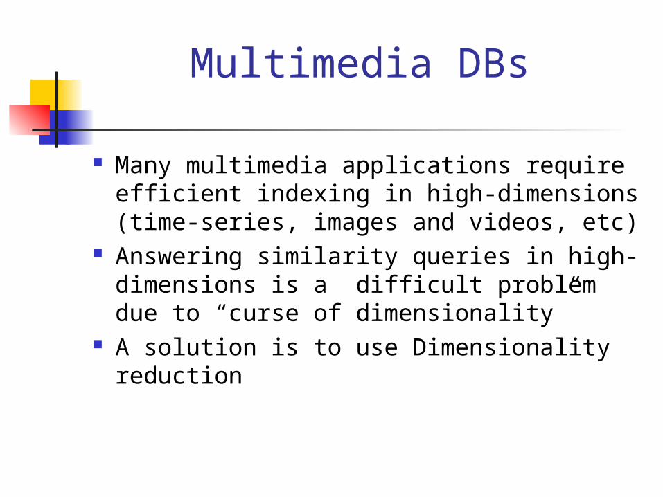
Multimedia DBs

Many multimedia applications require efficient indexing in high-dimensions (time-series, images and videos, etc)

Answering similarity queries in high-dimensions is a difficult problem due to “curse of dimensionality”

A solution is to use Dimensionality reduction

High-dimensional datasets

Range queries have very small selectivity Surface is everything Partitioning the space is not so easy: 2d

cells if we divide each dimension once Pair-wise distances of points is very

skewed

distance

freq

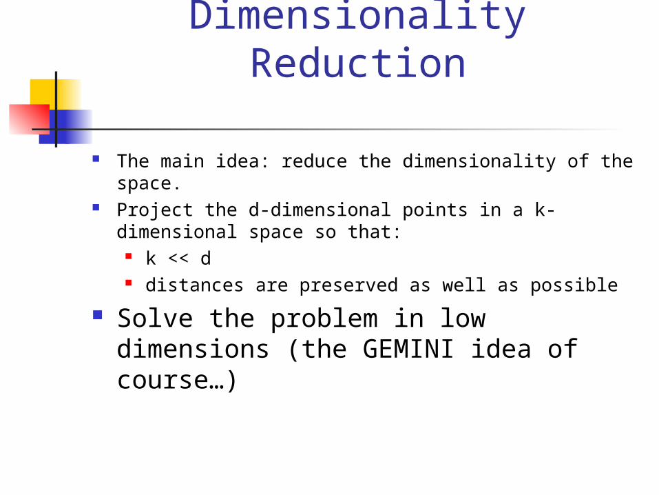
Dimensionality Reduction

The main idea: reduce the dimensionality of the space. Project the d-dimensional points in a k-dimensional

space so that: k << d distances are preserved as well as possible

Solve the problem in low dimensions (the GEMINI idea of course…)

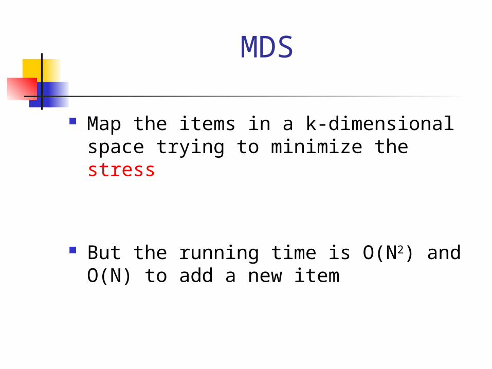
MDS

Map the items in a k-dimensional space trying to minimize the stress

But the running time is O(N2) and O(N) to add a new item

FastMap

Find two objects that are far away Project all points on the line the two objects define, to

get the first coordinate

FastMap - next iteration

Example

01100100100O5

10100100100O4

100100011O3

100100101O2

100100110O1

O5O4O3O2O1~100

~1

Example

Pivot Objects: O1 and O4 X1: O1:0, O2:0.005, O3:0.005, O4:100,

O5:99 For the second iteration pivots are: O2

and O5

Results

Documents /cosine similarity -> Euclidean distance (how?)

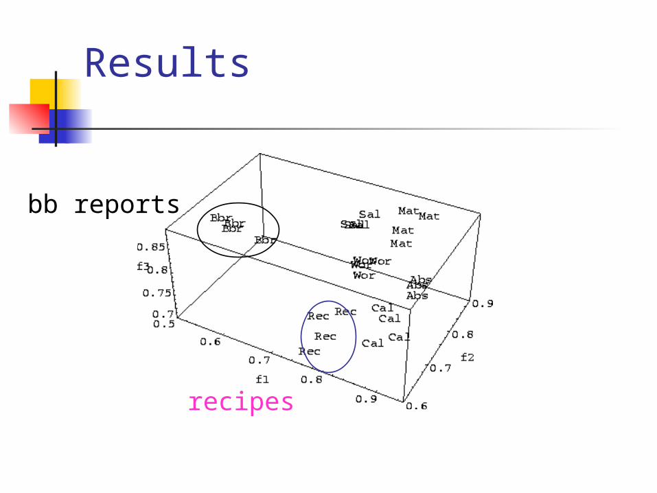
Results

recipes

bb reports

FastMap Extensions

If the original space is not a Euclidean space, then we may have a problem:

The projected distance may be a complex number!

A solution to that problem is to define: di(a,b) = sign(di(a,b)) (| di(a,b) |2)1/2

where, di(a,b) = di-1(a,b)2 – (xia-xb

i)2

Other DR methods

Using SVD and project the items on the first k eigenvectors

Random projections

SVD decomposition - the Karhunen-Loeve transform

Intuition: find the axis that shows the greatest variation, and project all points into this axis

f1

e1e2

f2

SVD: The mathematical formulation

Find the eigenvectors of the covariance matrix

These define the new space

Sort the eigenvalues in “goodness” order

f1

e1e2

f2

SVD: The mathematical formulation

Let A be the N x M matrix of N M-dimensional points The SVD decomposition of A is: = U x L x VT, But running time O(Nm2). How many I/Os?

Idea: Find the eigenvectors of C=ATA (MxM) If M<<N, then C can be kept in main memory and can

be constructed in one pass. (so we can find V and L) One more pass to construct U

SVD Cont’d

Advantages: Optimal dimensionality reduction (for linear

projections)

Disadvantages: Computationally hard, especially if the time series

are very long. Does not work for subsequence indexing

SVD Extensions

On-line approximation algorithm [Ravi Kanth et al, 1998]

Local diemensionality reduction: Cluster the time series, solve for each cluster [Chakrabarti and Mehrotra, 2000], [Thomasian et al]

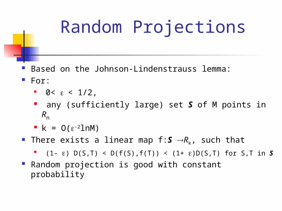
Random Projections

Based on the Johnson-Lindenstrauss lemma: For:

0< < 1/2, any (sufficiently large) set S of M points in Rn

k = O(-2lnM) There exists a linear map f:S Rk, such that

(1- ) D(S,T) < D(f(S),f(T)) < (1+ )D(S,T) for S,T in S Random projection is good with constant

probability

Random Projection: Application

Set k = O(e-2lnM) Select k random n-dimensional vectors (an approach is

to select k gaussian distributed vectors with variance 0 and mean value 1: N(1,0) )

Project the time series into the k vectors. The resulting k-dimensional space approximately

preserves the distances with high probability

Monte-Carlo algorithm: we do not know if correct

Random Projection

A very useful technique, Especially when used in conjunction with another

technique (for example SVD) Use Random projection to reduce the dimensionality

from thousands to hundred, then apply SVD to reduce dimensionality farther