Digitizing the Parthenon: Estimating Surface Reﬂectance ...ict.usc.edu/pubs/Digitizing the...

6Digitizing the Parthenon: Estimating SurfaceReflectance under Measured Natural Illumination

Paul Debevec, Chris Tchou, Andrew Gardner, Tim Hawkins, Charis Poullis, Jessi Stumpfel,Andrew Jones, Nathaniel Yun, Per Einarsson, Therese Lundgren, Marcos FajardoUniversity of Southern CaliforniaEmail: [email protected], [email protected],[email protected], [email protected],[email protected], [email protected],[email protected], corellian [email protected],[email protected], [email protected],[email protected]

Philippe MartinezEcole Normale SuperieureEmail: [email protected]

CONTENTS6.1 Introduction . . . . . . . . . . . . . . . . . . . . . . . . . . . . . . . . . . . . . . . . . . . . . . . . . . . . . . . . . . . . . . . . . . . . . . . . . . . . . . 1596.2 Background and Related Work . . . . . . . . . . . . . . . . . . . . . . . . . . . . . . . . . . . . . . . . . . . . . . . . . . . . . . . . . . . . . 1616.3 Data Acquisiton and Calibration . . . . . . . . . . . . . . . . . . . . . . . . . . . . . . . . . . . . . . . . . . . . . . . . . . . . . . . . . . 162

6.3.1 Camera Calibration . . . . . . . . . . . . . . . . . . . . . . . . . . . . . . . . . . . . . . . . . . . . . . . . . . . . . . . . . . . . . . . 1626.3.2 BRDF Measurement and Modeling . . . . . . . . . . . . . . . . . . . . . . . . . . . . . . . . . . . . . . . . . . . . . . . 1636.3.3 Natural Illumination Capture . . . . . . . . . . . . . . . . . . . . . . . . . . . . . . . . . . . . . . . . . . . . . . . . . . . . . 1666.3.4 3D Scanning . . . . . . . . . . . . . . . . . . . . . . . . . . . . . . . . . . . . . . . . . . . . . . . . . . . . . . . . . . . . . . . . . . . . . 1706.3.5 Photograph Acquisition and Alignment . . . . . . . . . . . . . . . . . . . . . . . . . . . . . . . . . . . . . . . . . . . . 171

6.4 Reflectometry . . . . . . . . . . . . . . . . . . . . . . . . . . . . . . . . . . . . . . . . . . . . . . . . . . . . . . . . . . . . . . . . . . . . . . . . . . . . 1726.4.1 General Algorithm . . . . . . . . . . . . . . . . . . . . . . . . . . . . . . . . . . . . . . . . . . . . . . . . . . . . . . . . . . . . . . . . 1726.4.2 Multiresolution Reflectance Solving . . . . . . . . . . . . . . . . . . . . . . . . . . . . . . . . . . . . . . . . . . . . . . 173

6.5 Results . . . . . . . . . . . . . . . . . . . . . . . . . . . . . . . . . . . . . . . . . . . . . . . . . . . . . . . . . . . . . . . . . . . . . . . . . . . . . . . . . . . 1766.6 Discussion and Future Work . . . . . . . . . . . . . . . . . . . . . . . . . . . . . . . . . . . . . . . . . . . . . . . . . . . . . . . . . . . . . . . 1776.7 Conclusion . . . . . . . . . . . . . . . . . . . . . . . . . . . . . . . . . . . . . . . . . . . . . . . . . . . . . . . . . . . . . . . . . . . . . . . . . . . . . . . 179

Acknowledgments . . . . . . . . . . . . . . . . . . . . . . . . . . . . . . . . . . . . . . . . . . . . . . . . . . . . . . . . . . . . . . . . . . . . . . . . 179Bibliography . . . . . . . . . . . . . . . . . . . . . . . . . . . . . . . . . . . . . . . . . . . . . . . . . . . . . . . . . . . . . . . . . . . . . . . . . . . . . 180

6.1 IntroductionDigitizing objects and environments from the real world has become an important part of creatingrealistic computer graphics. Capturing geometric models has become a common process through theuse of structured lighting, laser triangulation, and laser time-of-flight measurements. Recent projectssuch as [1–3] have shown that accurate and detailed geometric models can be acquired of real-worldobjects using these techniques.

159

© 2012 by Taylor & Francis Group, LLC

mailto:[email protected]












160 Digital Imaging for Cultural Heritage Preservation

To produce renderings of an object under changing lighting as well as viewpoint, it is necessaryto digitize not only the object’s geometry but also its reflectance properties: how each point of theobject reflects light. Digitizing reflectance properties has proven to be a complex problem, sincethese properties can vary across the surface of an object, and since the reflectance properties of evena single surface point can be complicated to express and measure. Some of the best results thathave been obtained [2, 4, 5] capture digital photographs of objects from a variety of viewing andillumination directions, and from these measurements estimate reflectance model parameters for eachsurface point.

Digitizing the reflectance properties of outdoor scenes can be more complicated than for objectssince it is more difficult to control the illumination and viewpoints of the surfaces. Surfaces aremost easily photographed from ground level rather than from a full range of angles. During thedaytime the illumination conditions in an environment change continuously. Finally, outdoor scenesgenerally exhibit significant mutual illumination between their surfaces, which must be accountedfor in the reflectance estimation process. Two recent pieces of work have made important inroadsinto this problem. In Yu at al. [6] estimated spatially varying reflectance properties of an outdoorbuilding based on fitting observations of the incident illumination to a sky model, and [7] estimatedreflectance properties of a room interior based on known light source positions and using a finiteelement radiosity technique to take surface interreflections into account.

In this paper, we describe a process that synthesizes previous results for digitizing geometryand reflectance and extends them to the context of digitizing a complex real-world scene observedunder arbitrary natural illumination. The data we acquire includes a geometric model of the sceneobtained through laser scanning, a set of photographs of the scene under various natural illuminationconditions, a corresponding set of measurements of the incident illumination for each photograph,and finally, a small set of Bi-directional Reflectance Distribution Function (BRDF) measurementsof representative surfaces within the scene. To estimate the scene’s reflectance properties, we usea global illumination algorithm to render the model from each of the photographed viewpoints asilluminated by the corresponding incident illumination measurements. We compare these renderingsto the photographs, and then iteratively update the surface reflectance properties to best correspondto the scene’s appearance in the photographs. Full BRDFs for the scene’s surfaces are inferred fromthe measured BRDF samples. The result is a set of estimated reflectance properties for each point inthe scene that most closely generates the scene’s appearance under all input illumination conditions.

While the process we describe leverages existing techniques, our work includes several novelcontributions. These include our incident illumination measurement process, which can measure thefull dynamic range of both sunlit and cloudy natural illumination conditions, a hand-held BRDFmeasurement process suitable for use in the field, and an iterative multiresolution inverse globalillumination process capable of estimating surface reflectance properties from multiple images forscenes with complex geometry seen under complex incident illumination.

The scene we digitize is the Parthenon in Athens, Greece, digitally laser scanned and pho-tographed in April 2003 in collaboration with the ongoing Acropolis Restoration project. Scaffoldingand equipment around the structure prevented the application of the process to the middle sectionof the temple, but we were able to derive models and reflectance parameters for both the East andWest facades. We validated the accuracy of our results by comparing our reflectance measurementsto ground truth measurements of specific surfaces around the site, and we generate renderings of themodel under novel lighting that are consistent with real photographs of the site. At the end of thepaper we discuss avenues for future work to increase the generality of these techniques. The work inthis chapter was first described as a Technical Report in [8].


Digitizing the Parthenon: Estimating Surface Reflectance under Measured Natural Illumination 161

6.2 Background and Related WorkThe process we present leverages previous results in 3D scanning, reflectance modeling, lightingrecovery, and reflectometry of objects and environments. Techniques for building 3D models frommultiple range scans generally involve first aligning the scans to each other [9,10], and then combiningthe scans into a consistent geometric model by either “zippering” the overlapping meshes [11] orusing volumetric merging [12] to create a new geometric mesh that optimizes its proximity to all ofthe available scans. In its simplest form, a point’s reflectance properties can be expressed in termsof its Lambertian surface color - usually an RGB triplet expressing the point’s red, green, and bluereflectance properties. More complex reflectance models can include parametric models of specularand retroflective components; some commonly used models are [13–15]. More generally, a point’sreflectance can be characterized in terms of its Bi-directional Reflectance Distribution Function(BRDF) [16], which is a 4D function that characterizes for each incident illumination direction thecomplete distribution of reflected illumination. Marschner et al. [17] proposed an efficient methodfor measuring a material’s BRDFs if a convex homogeneous sample is available. Recent work hasproposed models which also consider scattering of illumination within translucent materials [18].To estimate a scene’s reflectance properties, we use an incident illumination measurement process.Marschner et al. [19] recovered low-resolution incident illumination conditions by observing an objectwith known geometry and reflectance properties. Sato et al. [20] estimated incident illuminationconditions by observing the shadows cast from objects with known geometry. Debevec in [21]acquired high-resolution lighting environments by taking high dynamic range images [22] of amirrored sphere, but did not recover natural illumination environments where the sun was directlyvisible. We combine ideas from [19, 21] to record high-resolution incident illumination conditions incloudy, partly cloudy, and sunlit environments. Considerable recent work has presented techniquesto measure spatially-varying reflectance properties of objects. Marschner in [4] uses photographsof a 3D scanned object taken under point-light source illumination to estimate its spatially varyingdiffuse albedo. This work used a texture atlas system to store the surface colors of arbitrarily complexgeometry, which we also perform in our work. The work assumed that the object was Lambertian,and only considered local reflections of the illumination. Sato et al. [23] use a similar sort of datasetto compute a spatially-varying diffuse component and a sparsely sampled specular component ofan object. Rushmeier et al. [2] use a photometric stereo technique [24, 25] to estimate spatiallyvarying Lambertian color as well as improved surface normals for the geometry. Rocchini et al. [26]use this technique to compute diffuse texture maps for 3D scanned objects from multiple images.Debevec et al. [27] use a dense set of illumination directions to estimate spatially-varying diffuseand specular parameters and surface normals. Lensch et al. [5] presents an advanced techniquefor recovering spatially-varying BRDFs of real-world objects, performing principal componentanalysis of relatively sparse lighting and viewing directions to cluster the object’s surfaces intopatches of similar reflectance. In this way, many reflectance observations of the object as a wholeare used to estimate spatially-varying BRDF models for surfaces seen from limited viewing andlighting directions. Our reflectance modeling technique is less general, but adapts ideas from thiswork to estimate spatially-varying non-Lambertian reflectance properties of outdoor scenes observedunder natural illumination conditions, and we also account for mutual illumination. Capturing thereflectance properties of surfaces in large-scale environments can be more complex, since it canbe harder to control the lighting conditions on the surfaces and the viewpoints from which theyare photographed. Yu et al. [6] solve for the reflectance properties of a polygonal model of anoutdoor scene modeled with photogrammetry. The technique used photographs taken under clearsky conditions, fitting a small number of radiance measurements to a parameterized sky model. Theprocess estimated spatially varying diffuse and piecewise constant specular parameters, but did notconsider retroreflective components. The process derived two pseudo-BRDFs for each surface, one



according to its reflectance of light from the sun and one according to its reflectance of light from thesky and environment. This allowed more general spectral modeling but required every surface tobe observed under direct sunlight in at least one photograph, which we do not require. Using roominteriors [7, 28, 29] estimate spatially varying diffuse and piecewise constant specular parametersusing inverse global illumination. The techniques used knowledge of the position and intensity ofthe scene’s light sources, using global illumination to account for the mutual illumination betweenthe scene’s surfaces. Our work combines and extends aspects of each of these techniques: we usepictures of our scene under natural illumination conditions, but we image the illumination directly inorder to use photographs taken in sunny, partly sunny, or cloudy conditions. We infer non-Lambertianreflectance from sampled surface BRDFs. We do not consider full-spectral reflectance, but havefound RGB imaging to be sufficiently accurate for the natural illumination and reflectance propertiesrecorded in this work. We provide comparisons to ground truth reflectance for several surfaces withinthe scene. Finally, we use a more general Monte-Carlo global illumination algorithm to performour inverse rendering, and we employ a multiresolution geometry technique to efficiently process acomplex laser-scanned model.

6.3 Data Acquisiton and Calibration6.3.1 Camera CalibrationIn this work we used a Canon EOS D30 and a Canon EOS 1Ds digital camera, which were calibratedgeometrically and radiometrically. For geometric calibration, we used the Camera CalibrationToolbox for Matlab [30] which uses techniques from [31]. Since changing the focus of a lens usuallychanges its focal length, we calibrated our lenses at chosen fixed focal lengths. The main lens used forphotographing the environment was a 24mm lens focused at infinity. Since a small calibration objectheld near this lens would be out of focus, we built a larger calibration object 1.2m × 2.1m from analuminum honeycomb panel with a 5cm square checkerboard pattern applied (Figure 6.1(a)). Thoughnearly all images were acquired at f/8 aperture, we verified that the camera intrinsic parametersvaried insignificantly (less than 0.05%) with changes of f/stop from f/2.8 to f/22. In this workwe wished to obtain radiometrically linear pixel values that would be consistent for images takenwith different cameras, lenses, shutter speeds, and f/stop. We verified that the “RAW” 12-bit datafrom the cameras was linear using three methods: we photographed a gray scale calibration chart,we used the radiometric self-calibration technique of [22], and we verified that pixel values wereproportional to exposure times for a static scene. From this we found that the RAW pixel valuesexhibited linear response to within 0.1% for values up to 3,000 out of 4,095, after which saturationappeared to reduce pixel sensitivity. We ignored values outside of this linear range, and we usedmultiple exposures to increase the effective dynamic range of the camera when necessary.

Most lenses exhibit a radial intensity falloff, producing dimmer pixel values at the periphery ofthe image. We mounted each camera on a Kaidan nodal rotation head and photographed a diffuse disklight source at an array of positions for each lens at each f/stop used for data capture (Figure 6.1(b)).From these intensities recorded at different image points, we fit a radially symmetric 6th order evenpolynomial to model the falloff curve and produce a flat-field response function, normalized to unitresponse at the image center.

Each digital camera used had minor variations in sensitivity and color response. We calibratedthese variations by photographing a MacBeth color checker chart under natural illumination witheach camera, lens, and f/stop combination, and solved for the best 3× 3 color matrix to converteach image into the same color space. Finally we used a utility for converting RAW images tofloating-point images using the EXIF metadata for camera model, lens, ISO, f/stop, and shutter speed



(a) (b) (c)

FIGURE 6.1(a) 1.2m × 2.1m geometric calibration object; (b) Lens falloff measurements for 24mm lens at f/8;(c) Lens falloff curve for (b).

to apply the appropriate radiometric scaling factors and matrices. These images were organized in aPostGreSQL database for convenient access.

6.3.2 BRDF Measurement and ModelingIn this work we measure BRDFs of a set of representative surface samples, which we use to form themost plausible BRDFs for the rest of the scene. Our relatively simple technique is motivated by theprincipal component analyses of reflectance properties used in [5, 32], except that we choose ourbasis BRDFs manually. Choosing the principal BRDFs in this way meant that BRDF data collectedunder controlled illumination could be taken for a small area of the site, while the large-scale scenecould be photographed under a limited set of natural illumination conditions.

Data Collection and RegistrationThe site used in this work is composed entirely of marble, but its surfaces have been subject to

different discoloration processes yielding significant reflectance variations. We located an accessible30cm × 30cm surface that exhibited a range of coloration properties representative of the site. Sincemeasuring the reflectance properties of this surface required controlled illumination conditions, weperformed these measurements during our limited nighttime access to the site and used a BRDFmeasurement technique that could be executed quickly.

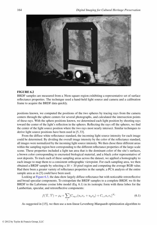
The BRDF measurement setup (Figure 6.2), includes a hand-held light source and camera, anduses a frame placed around the sample area that allows the lighting and viewing directions to beestimated from the images taken with the camera. The frame contains fiducial markers at each cornerof the frame’s aperture from which the camera’s position can be estimated, and two glossy blackplastic spheres used to determine the 3D position of the light source. Finally, the device includesa diffuse white reflectance standard parallel to the sample area for determining the intensity of thelight source.

The light source chosen was a 1,000W halogen source mounted in a small diffuser box, heldapproximately 3m from the surface. Our capture assumed that the surfaces exhibited isotropicreflection, requiring the light source to be moved only within a single plane of incidence. We placedthe light source in four consecutive positions of 0◦, 30◦, 50◦, 75◦, and for each took hand-heldphotographs at a distance of approximately 2m from twenty directions distributed on the incidenthemisphere, taking care to sample the specular and retroreflective directions with a greater numberof observations. Dark clothing was worn to reduce stray illumination on the sample. The full captureprocess involving 83 photographs required forty minutes.

Data Analysis and Reflectance Model FittingTo calculate the viewing and lighting directions, we first determined the position of the camera

from the known 3D positions of the four fiducial markers using photogrammetry. With the camera



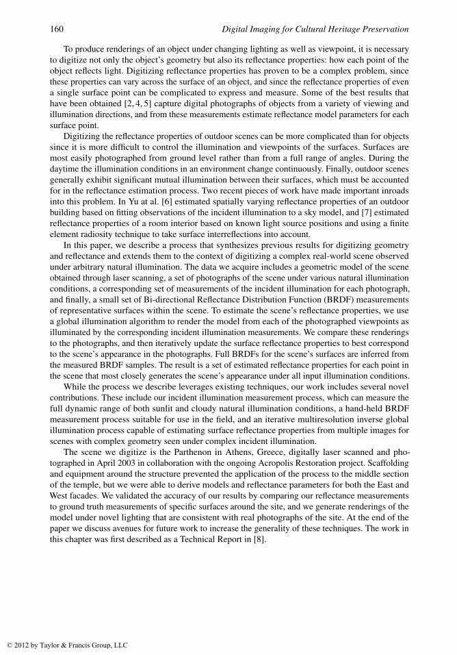
FIGURE 6.2BRDF samples are measured from a 30cm square region exhibiting a representative set of surfacereflectance properties. The technique used a hand-held light source and camera and a calibrationframe to acquire the BRDF data quickly.

positions known, we computed the positions of the two spheres by tracing rays from the cameracenters through the sphere centers for several photographs, and calculated the intersection pointsof these rays. With the sphere positions known, we determined each light position by shooting raystoward the center of the light’s reflection in the spheres. Reflecting the rays off the spheres, we findthe center of the light source position where the two rays most nearly intersect. Similar techniques toderive light source positions have been used in [5, 33].

From the diffuse white reflectance standard, the incoming light source intensity for each imagecould be determined. By dividing the overall image intensity by the color of the reflectance standard,all images were normalized by the incoming light source intensity. We then chose three different areaswithin the sampling region best corresponding to the different reflectance properties of the large-scalescene. These properties included a light tan area that is the dominant color of the site’s surfaces,a brown color corresponding to encrusted biological material, and a black color representative ofsoot deposits. To track each of these sampling areas across the dataset, we applied a homography toeach image to map them to a consistent orthographic viewpoint. For each sampling area, we thenobtained a BRDF sample by selecting a 30× 30 pixel region and computing the average RGB value.Had there been a greater variety of reflectance properties in the sample, a PCA analysis of the entiresample area as in [5] could have been used.

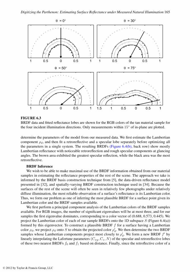
Looking at Figure 6.3, the data show largely diffuse reflectance but with noticeable retroreflectiveand broad specular components. To extrapolate the BRDF samples to a complete BRDF, we fit theBRDF to the Lafortune cosine lobe model (Eq. 6.1) in its isotropic form with three lobes for theLambertian, specular, and retroreflective components:

f(−→u ,−→v ) = ρd +�

i

[Cxy,i(uxvx + uyvy) + Cz,iuzvz]Ni (6.1)

As suggested in [15], we then use a non-linear Levenberg-Marquardt optimization algorithm to



FIGURE 6.3BRDF data and fitted reflectance lobes are shown for the RGB colors of the tan material sample forthe four incident illumination directions. Only measurements within 15◦ of in-plane are plotted.

determine the parameters of the model from our measured data. We first estimate the Lambertiancomponent ρd, and then fit a retroreflective and a specular lobe separately before optimizing allthe parameters in a single system. The resulting BRDFs (Figure 6.4(b), back row) show mostlyLambertian reflectance with noticeable retroreflection and rough specular components at glancingangles. The brown area exhibited the greatest specular reflection, while the black area was the mostretroreflective.

BRDF InferenceWe wish to be able to make maximal use of the BRDF information obtained from our material

samples in estimating the reflectance properties of the rest of the scene. The approach we take isinformed by the BRDF basis construction technique from [5], the data-driven reflectance modelpresented in [32], and spatially-varying BRDF construction technique used in [34]. Because thesurfaces of the rest of the scene will often be seen in relatively few photographs under relativelydiffuse illumination, the most reliable observation of a surface’s reflectance is its Lambertian color.Thus, we form our problem as one of inferring the most plausible BRDF for a surface point given itsLambertian color and the BRDF samples available.

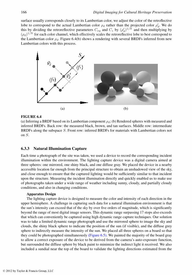
We first perform a principal component analysis of the Lambertian colors of the BRDF samplesavailable. For RGB images, the number of significant eigenvalues will be at most three, and for oursamples the first eigenvalue dominates, corresponding to a color vector of (0.688, 0.573, 0.445). Weproject the Lambertian color of each of our sample BRDFs onto the 1D subspace S (Figure 6.4(a))formed by this eigenvector. To construct a plausible BRDF f for a surface having a Lambertiancolor ρd, we project ρd onto S to obtain the projected color ρ�

d. We then determine the two BRDFsamples whose Lambertian components project most closely to ρ�

d. We form a new BRDF f � bylinearly interpolating the Lafortune parameters (Cxy, Cz, N) of the specular and retroreflective lobesof these two nearest BRDFs f0 and f1 based on distance. Finally, since the retroflective color of a



surface usually corresponds closely to its Lambertian color, we adjust the color of the retroflectivelobe to correspond to the actual Lambertian color ρd rather than the projected color ρ�

d. We dothis by dividing the retroreflective parameters Cxy and Cz by (ρ�

d)1/N and then multiplying by

(ρd)1/N for each color channel, which effectively scales the retroreflective lobe to best correspond tothe Lambertian color ρd. Figure 6.4(b) shows a rendering with several BRDFs inferred from newLambertian colors with this process.

(a) (b)

FIGURE 6.4(a) Inferring a BRDF based on its Lambertian component ρd; (b) Rendered spheres with measured andinferred BRDFs. Back row: the measured black, brown, and tan surfaces. Middle row: intermediateBRDFs along the subspace S. Front row: inferred BRDFs for materials with Lambertian colors noton S.

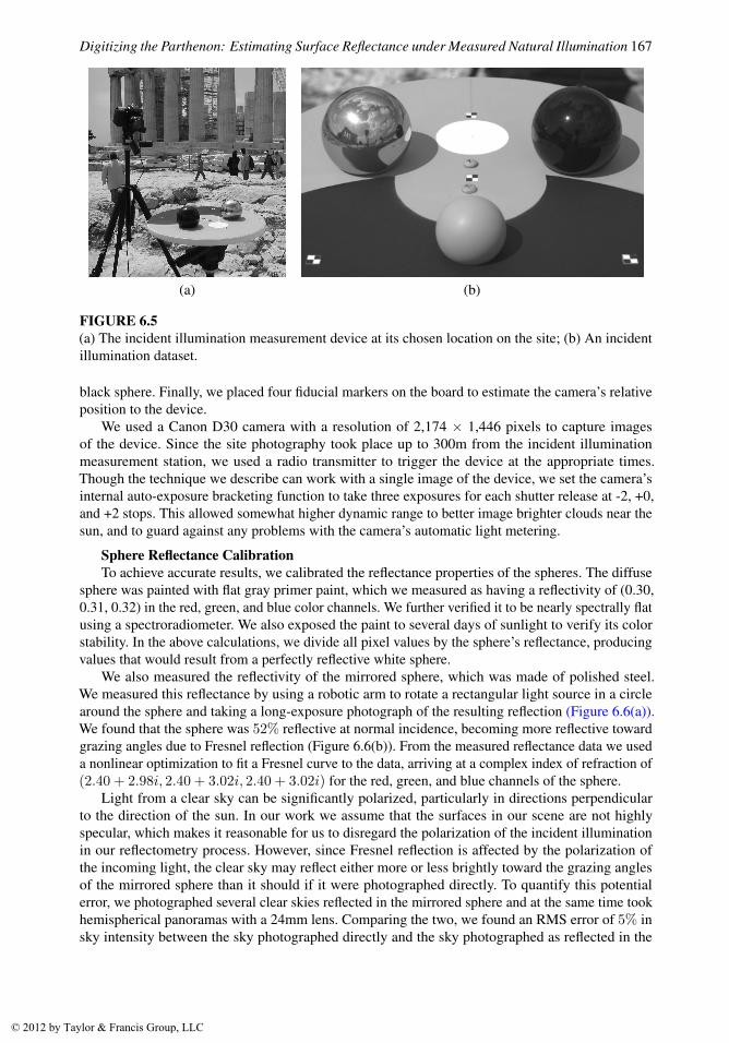
6.3.3 Natural Illumination CaptureEach time a photograph of the site was taken, we used a device to record the corresponding incidentillumination within the environment. The lighting capture device was a digital camera aimed atthree spheres: one mirrored, one shiny black, and one diffuse gray. We placed the device in a nearbyaccessible location far enough from the principal structure to obtain an unshadowed view of the sky,and close enough to ensure that the captured lighting would be sufficiently similar to that incidentupon the structure. Measuring the incident illumination directly and quickly enabled us to make useof photographs taken under a wide range of weather including sunny, cloudy, and partially cloudyconditions, and also in changing conditions.

Apparatus DesignThe lighting capture device is designed to measure the color and intensity of each direction in the

upper hemisphere. A challenge in capturing such data for a natural illumination environment is thatthe sun’s intensity can exceed that of the sky by over five orders of magnitude, which is significantlybeyond the range of most digital image sensors. This dynamic range surpassing 17 stops also exceedsthat which can conveniently be captured using high dynamic range capture techniques. Our solutionwas to take a limited dynamic range photograph and use the mirrored sphere to image the sky andclouds, the shiny black sphere to indicate the position of the sun (if visible), and the diffuse greysphere to indirectly measure the intensity of the sun. We placed all three spheres on a board so thatthey could be photographed simultaneously (Figure 6.5). We painted the majority of the board grayto allow a correct exposure of the device to be derived from the camera’s auto-exposure function,but surrounded the diffuse sphere by black paint to minimize the indirect light it received. We alsoincluded a sundial near the top of the board to validate the lighting directions estimated from the



(a) (b)

FIGURE 6.5(a) The incident illumination measurement device at its chosen location on the site; (b) An incidentillumination dataset.

black sphere. Finally, we placed four fiducial markers on the board to estimate the camera’s relativeposition to the device.

We used a Canon D30 camera with a resolution of 2,174 × 1,446 pixels to capture imagesof the device. Since the site photography took place up to 300m from the incident illuminationmeasurement station, we used a radio transmitter to trigger the device at the appropriate times.Though the technique we describe can work with a single image of the device, we set the camera’sinternal auto-exposure bracketing function to take three exposures for each shutter release at -2, +0,and +2 stops. This allowed somewhat higher dynamic range to better image brighter clouds near thesun, and to guard against any problems with the camera’s automatic light metering.

Sphere Reflectance CalibrationTo achieve accurate results, we calibrated the reflectance properties of the spheres. The diffuse

sphere was painted with flat gray primer paint, which we measured as having a reflectivity of (0.30,0.31, 0.32) in the red, green, and blue color channels. We further verified it to be nearly spectrally flatusing a spectroradiometer. We also exposed the paint to several days of sunlight to verify its colorstability. In the above calculations, we divide all pixel values by the sphere’s reflectance, producingvalues that would result from a perfectly reflective white sphere.

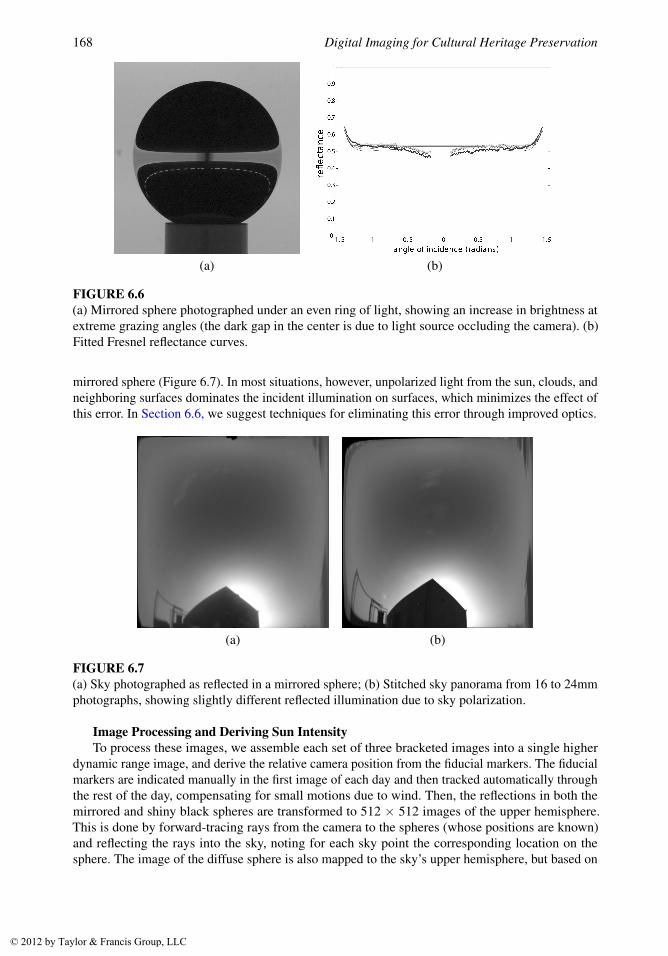
We also measured the reflectivity of the mirrored sphere, which was made of polished steel.We measured this reflectance by using a robotic arm to rotate a rectangular light source in a circlearound the sphere and taking a long-exposure photograph of the resulting reflection (Figure 6.6(a)).We found that the sphere was 52% reflective at normal incidence, becoming more reflective towardgrazing angles due to Fresnel reflection (Figure 6.6(b)). From the measured reflectance data we useda nonlinear optimization to fit a Fresnel curve to the data, arriving at a complex index of refraction of(2.40 + 2.98i, 2.40 + 3.02i, 2.40 + 3.02i) for the red, green, and blue channels of the sphere.

Light from a clear sky can be significantly polarized, particularly in directions perpendicularto the direction of the sun. In our work we assume that the surfaces in our scene are not highlyspecular, which makes it reasonable for us to disregard the polarization of the incident illuminationin our reflectometry process. However, since Fresnel reflection is affected by the polarization ofthe incoming light, the clear sky may reflect either more or less brightly toward the grazing anglesof the mirrored sphere than it should if it were photographed directly. To quantify this potentialerror, we photographed several clear skies reflected in the mirrored sphere and at the same time tookhemispherical panoramas with a 24mm lens. Comparing the two, we found an RMS error of 5% insky intensity between the sky photographed directly and the sky photographed as reflected in the



(a) (b)

FIGURE 6.6(a) Mirrored sphere photographed under an even ring of light, showing an increase in brightness atextreme grazing angles (the dark gap in the center is due to light source occluding the camera). (b)Fitted Fresnel reflectance curves.

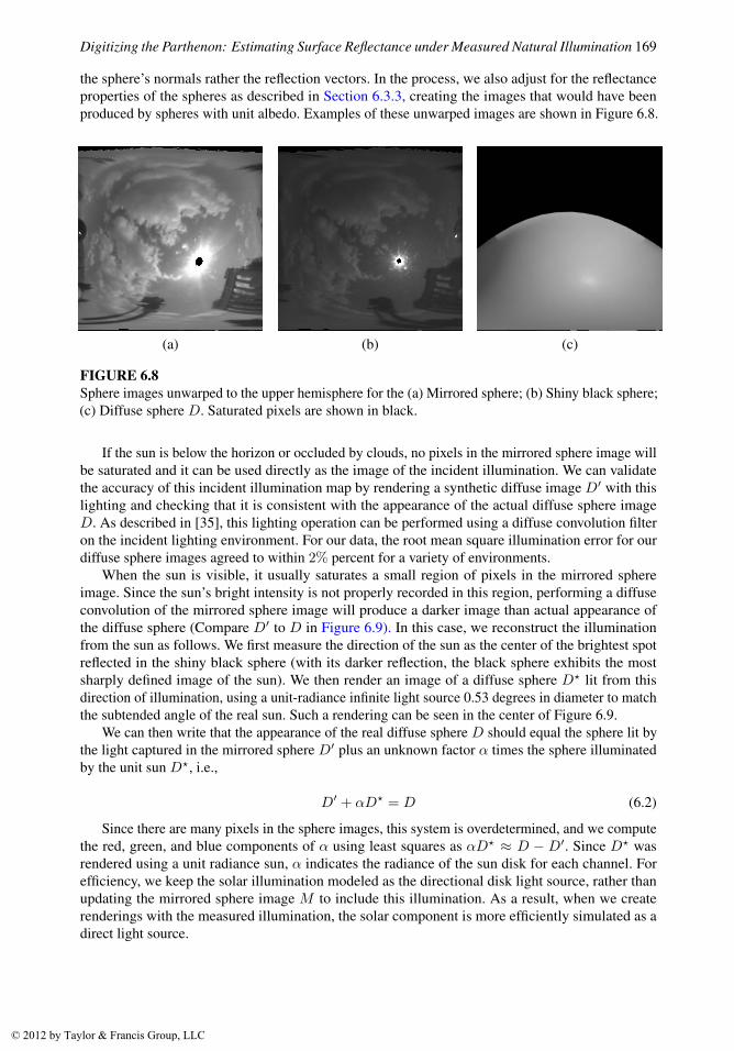
mirrored sphere (Figure 6.7). In most situations, however, unpolarized light from the sun, clouds, andneighboring surfaces dominates the incident illumination on surfaces, which minimizes the effect ofthis error. In Section 6.6, we suggest techniques for eliminating this error through improved optics.

(a) (b)

FIGURE 6.7(a) Sky photographed as reflected in a mirrored sphere; (b) Stitched sky panorama from 16 to 24mmphotographs, showing slightly different reflected illumination due to sky polarization.

Image Processing and Deriving Sun IntensityTo process these images, we assemble each set of three bracketed images into a single higher

dynamic range image, and derive the relative camera position from the fiducial markers. The fiducialmarkers are indicated manually in the first image of each day and then tracked automatically throughthe rest of the day, compensating for small motions due to wind. Then, the reflections in both themirrored and shiny black spheres are transformed to 512 × 512 images of the upper hemisphere.This is done by forward-tracing rays from the camera to the spheres (whose positions are known)and reflecting the rays into the sky, noting for each sky point the corresponding location on thesphere. The image of the diffuse sphere is also mapped to the sky’s upper hemisphere, but based on



the sphere’s normals rather the reflection vectors. In the process, we also adjust for the reflectanceproperties of the spheres as described in Section 6.3.3, creating the images that would have beenproduced by spheres with unit albedo. Examples of these unwarped images are shown in Figure 6.8.

(a) (b) (c)

FIGURE 6.8Sphere images unwarped to the upper hemisphere for the (a) Mirrored sphere; (b) Shiny black sphere;(c) Diffuse sphere D. Saturated pixels are shown in black.

If the sun is below the horizon or occluded by clouds, no pixels in the mirrored sphere image willbe saturated and it can be used directly as the image of the incident illumination. We can validatethe accuracy of this incident illumination map by rendering a synthetic diffuse image D� with thislighting and checking that it is consistent with the appearance of the actual diffuse sphere imageD. As described in [35], this lighting operation can be performed using a diffuse convolution filteron the incident lighting environment. For our data, the root mean square illumination error for ourdiffuse sphere images agreed to within 2% percent for a variety of environments.

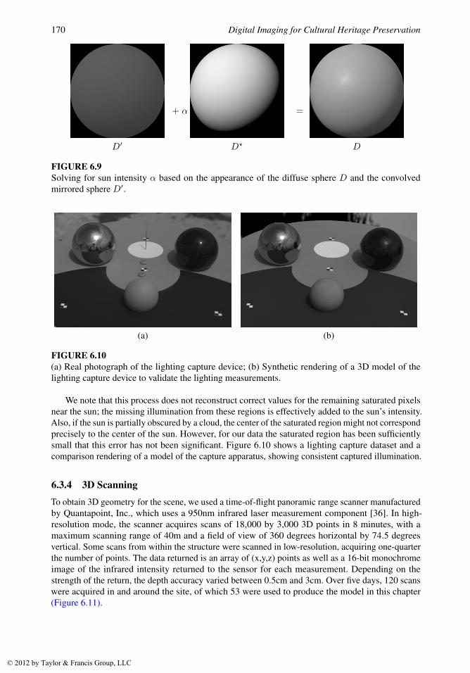
When the sun is visible, it usually saturates a small region of pixels in the mirrored sphereimage. Since the sun’s bright intensity is not properly recorded in this region, performing a diffuseconvolution of the mirrored sphere image will produce a darker image than actual appearance ofthe diffuse sphere (Compare D� to D in Figure 6.9). In this case, we reconstruct the illuminationfrom the sun as follows. We first measure the direction of the sun as the center of the brightest spotreflected in the shiny black sphere (with its darker reflection, the black sphere exhibits the mostsharply defined image of the sun). We then render an image of a diffuse sphere D� lit from thisdirection of illumination, using a unit-radiance infinite light source 0.53 degrees in diameter to matchthe subtended angle of the real sun. Such a rendering can be seen in the center of Figure 6.9.

We can then write that the appearance of the real diffuse sphere D should equal the sphere lit bythe light captured in the mirrored sphere D� plus an unknown factor α times the sphere illuminatedby the unit sun D�, i.e.,

D� + αD� = D (6.2)

Since there are many pixels in the sphere images, this system is overdetermined, and we computethe red, green, and blue components of α using least squares as αD� ≈ D − D�. Since D� wasrendered using a unit radiance sun, α indicates the radiance of the sun disk for each channel. Forefficiency, we keep the solar illumination modeled as the directional disk light source, rather thanupdating the mirrored sphere image M to include this illumination. As a result, when we createrenderings with the measured illumination, the solar component is more efficiently simulated as adirect light source.



+ α =

D� D� D

FIGURE 6.9Solving for sun intensity α based on the appearance of the diffuse sphere D and the convolvedmirrored sphere D�.

(a) (b)

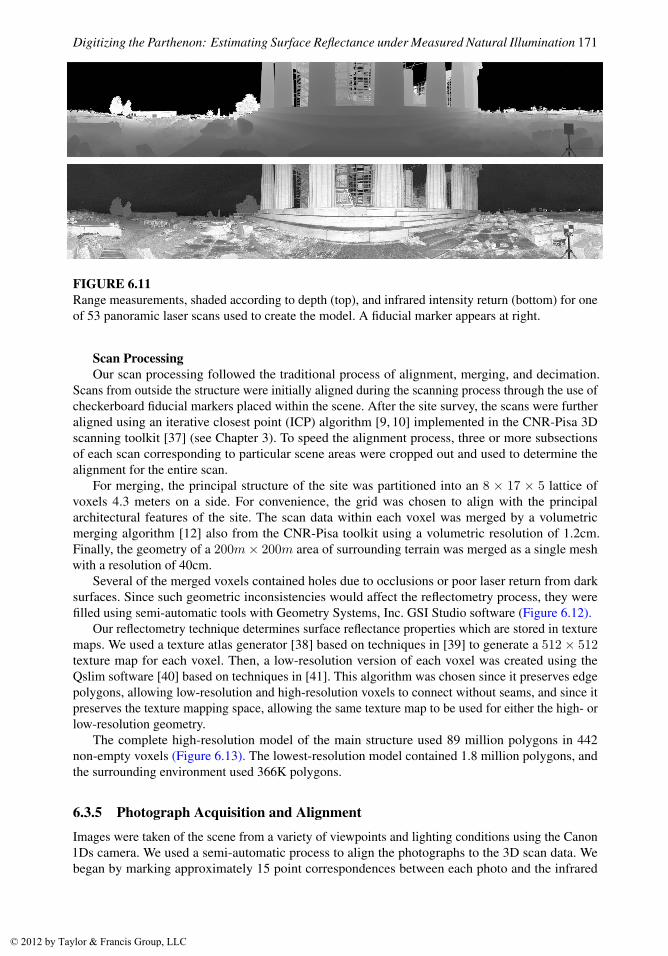
FIGURE 6.10(a) Real photograph of the lighting capture device; (b) Synthetic rendering of a 3D model of thelighting capture device to validate the lighting measurements.

We note that this process does not reconstruct correct values for the remaining saturated pixelsnear the sun; the missing illumination from these regions is effectively added to the sun’s intensity.Also, if the sun is partially obscured by a cloud, the center of the saturated region might not correspondprecisely to the center of the sun. However, for our data the saturated region has been sufficientlysmall that this error has not been significant. Figure 6.10 shows a lighting capture dataset and acomparison rendering of a model of the capture apparatus, showing consistent captured illumination.

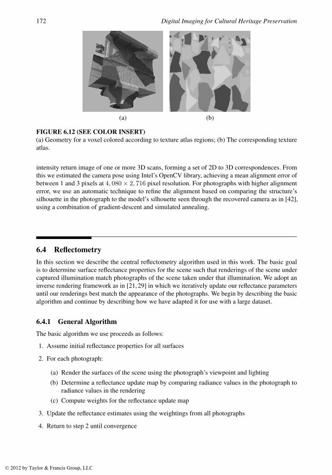
6.3.4 3D ScanningTo obtain 3D geometry for the scene, we used a time-of-flight panoramic range scanner manufacturedby Quantapoint, Inc., which uses a 950nm infrared laser measurement component [36]. In high-resolution mode, the scanner acquires scans of 18,000 by 3,000 3D points in 8 minutes, with amaximum scanning range of 40m and a field of view of 360 degrees horizontal by 74.5 degreesvertical. Some scans from within the structure were scanned in low-resolution, acquiring one-quarterthe number of points. The data returned is an array of (x,y,z) points as well as a 16-bit monochromeimage of the infrared intensity returned to the sensor for each measurement. Depending on thestrength of the return, the depth accuracy varied between 0.5cm and 3cm. Over five days, 120 scanswere acquired in and around the site, of which 53 were used to produce the model in this chapter(Figure 6.11).



FIGURE 6.11Range measurements, shaded according to depth (top), and infrared intensity return (bottom) for oneof 53 panoramic laser scans used to create the model. A fiducial marker appears at right.

Scan ProcessingOur scan processing followed the traditional process of alignment, merging, and decimation.

Scans from outside the structure were initially aligned during the scanning process through the use ofcheckerboard fiducial markers placed within the scene. After the site survey, the scans were furtheraligned using an iterative closest point (ICP) algorithm [9, 10] implemented in the CNR-Pisa 3Dscanning toolkit [37] (see Chapter 3). To speed the alignment process, three or more subsectionsof each scan corresponding to particular scene areas were cropped out and used to determine thealignment for the entire scan.

For merging, the principal structure of the site was partitioned into an 8 × 17 × 5 lattice ofvoxels 4.3 meters on a side. For convenience, the grid was chosen to align with the principalarchitectural features of the site. The scan data within each voxel was merged by a volumetricmerging algorithm [12] also from the CNR-Pisa toolkit using a volumetric resolution of 1.2cm.Finally, the geometry of a 200m× 200m area of surrounding terrain was merged as a single meshwith a resolution of 40cm.

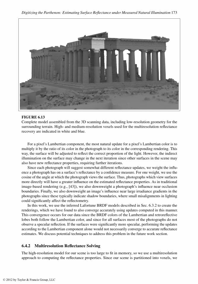
Several of the merged voxels contained holes due to occlusions or poor laser return from darksurfaces. Since such geometric inconsistencies would affect the reflectometry process, they werefilled using semi-automatic tools with Geometry Systems, Inc. GSI Studio software (Figure 6.12).

Our reflectometry technique determines surface reflectance properties which are stored in texturemaps. We used a texture atlas generator [38] based on techniques in [39] to generate a 512× 512texture map for each voxel. Then, a low-resolution version of each voxel was created using theQslim software [40] based on techniques in [41]. This algorithm was chosen since it preserves edgepolygons, allowing low-resolution and high-resolution voxels to connect without seams, and since itpreserves the texture mapping space, allowing the same texture map to be used for either the high- orlow-resolution geometry.

The complete high-resolution model of the main structure used 89 million polygons in 442non-empty voxels (Figure 6.13). The lowest-resolution model contained 1.8 million polygons, andthe surrounding environment used 366K polygons.

6.3.5 Photograph Acquisition and AlignmentImages were taken of the scene from a variety of viewpoints and lighting conditions using the Canon1Ds camera. We used a semi-automatic process to align the photographs to the 3D scan data. Webegan by marking approximately 15 point correspondences between each photo and the infrared



(a) (b)

FIGURE 6.12 (SEE COLOR INSERT)(a) Geometry for a voxel colored according to texture atlas regions; (b) The corresponding textureatlas.

intensity return image of one or more 3D scans, forming a set of 2D to 3D correspondences. Fromthis we estimated the camera pose using Intel’s OpenCV library, achieving a mean alignment error ofbetween 1 and 3 pixels at 4, 080× 2, 716 pixel resolution. For photographs with higher alignmenterror, we use an automatic technique to refine the alignment based on comparing the structure’ssilhouette in the photograph to the model’s silhouette seen through the recovered camera as in [42],using a combination of gradient-descent and simulated annealing.

6.4 ReflectometryIn this section we describe the central reflectometry algorithm used in this work. The basic goalis to determine surface reflectance properties for the scene such that renderings of the scene undercaptured illumination match photographs of the scene taken under that illumination. We adopt aninverse rendering framework as in [21, 29] in which we iteratively update our reflectance parametersuntil our renderings best match the appearance of the photographs. We begin by describing the basicalgorithm and continue by describing how we have adapted it for use with a large dataset.

6.4.1 General AlgorithmThe basic algorithm we use proceeds as follows:

1. Assume initial reflectance properties for all surfaces

2. For each photograph:

(a) Render the surfaces of the scene using the photograph’s viewpoint and lighting(b) Determine a reflectance update map by comparing radiance values in the photograph to

radiance values in the rendering(c) Compute weights for the reflectance update map

3. Update the reflectance estimates using the weightings from all photographs

4. Return to step 2 until convergence



FIGURE 6.13Complete model assembled from the 3D scanning data, including low-resolution geometry for thesurrounding terrain. High- and medium-resolution voxels used for the multiresolution reflectancerecovery are indicated in white and blue.

For a pixel’s Lambertian component, the most natural update for a pixel’s Lambertian color is tomultiply it by the ratio of its color in the photograph to its color in the corresponding rendering. Thisway, the surface will be adjusted to reflect the correct proportion of the light. However, the indirectillumination on the surface may change in the next iteration since other surfaces in the scene mayalso have new reflectance properties, requiring further iterations.

Since each photograph will suggest somewhat different reflectance updates, we weight the influ-ence a photograph has on a surface’s reflectance by a confidence measure. For one weight, we use thecosine of the angle at which the photograph views the surface. Thus, photographs which view surfacesmore directly will have a greater influence on the estimated reflectance properties. As in traditionalimage-based rendering (e.g., [43]), we also downweight a photograph’s influence near occlusionboundaries. Finally, we also downweight an image’s influence near large irradiance gradients in thephotographs since these typically indicate shadow boundaries, where small misalignments in lightingcould significantly affect the reflectometry.

In this work, we use the inferred Lafortune BRDF models described in Sec. 6.3.2 to create therenderings, which we have found to also converge accurately using updates computed in this manner.This convergence occurs for our data since the BRDF colors of the Lambertian and retroreflectivelobes both follow the Lambertian color, and since for all surfaces most of the photographs do notobserve a specular reflection. If the surfaces were significantly more specular, performing the updatesaccording to the Lambertian component alone would not necessarily converge to accurate reflectanceestimates. We discuss potential techniques to address this problem in the future work section.

6.4.2 Multiresolution Reflectance SolvingThe high-resolution model for our scene is too large to fit in memory, so we use a multiresolutionapproach to computing the reflectance properties. Since our scene is partitioned into voxels, we



can compute reflectance property updates one voxel at a time. However, we must still model theeffect of shadowing and indirect illumination for the rest of the scene. Fortunately, lower-resolutiongeometry can work well for this purpose. In our work, we use full-resolution geometry (approx.800K triangles) for the voxel being computed, medium-resolution geometry (approx. 160K triangles)for the immediately neighboring voxels, and low-resolution geometry (approx. 40K triangles) for theremaining voxels in the scene. The surrounding terrain is kept at a low resolution of 370K triangles.The multiresolution approach results in over a 90% data reduction in scene complexity during thereflectometry of any given voxel.

Our global illumination rendering system was originally designed to produce 2D images of ascene for a given camera viewpoint using path tracing [44]. We modified the system to include anew function for computing surface radiance for any point in the scene radiating toward any viewingposition. This allows the process of computing reflectance properties for a voxel to be done byiterating over the texture map space for that voxel. For efficiency, for each pixel in the voxel’stexture space, we cache the position and surface normal of the model corresponding to that texturecoordinate, storing these results in two additional floating-point texture maps.

1. Assume initial reflectance properties for all surfaces.

2. For each voxel V :

• Load V at high resolution, V ’s neighbors at medium resolution, and the rest of the modelat low resolution.

• For each pixel p in V ’s texture space:– For each photograph I:

∗ Determine if p’s surface is visible to I’s camera. If not, break. If so, determinethe weight for this image based on the visibility angle, and note pixel q in Icorresponding to p’s projection into I .

∗ Compute the radiance l of p’s surface in the direction of I’s camera under I’sillumination.

∗ Determine an updated surface reflectance by comparing the radiance in the imageat q to the rendered radiance l.

– Assign the new surface reflectance for p as the weighted average of the updatedreflectances from each I .

3. Return to step 2 until convergence

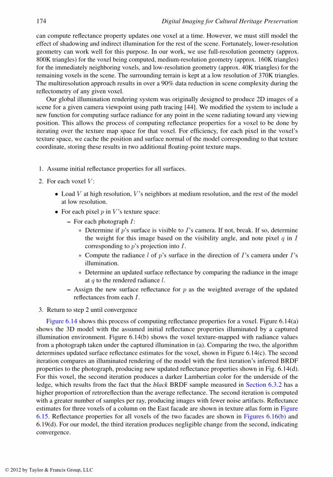
Figure 6.14 shows this process of computing reflectance properties for a voxel. Figure 6.14(a)shows the 3D model with the assumed initial reflectance properties illuminated by a capturedillumination environment. Figure 6.14(b) shows the voxel texture-mapped with radiance valuesfrom a photograph taken under the captured illumination in (a). Comparing the two, the algorithmdetermines updated surface reflectance estimates for the voxel, shown in Figure 6.14(c). The seconditeration compares an illuminated rendering of the model with the first iteration’s inferred BRDFproperties to the photograph, producing new updated reflectance properties shown in Fig. 6.14(d).For this voxel, the second iteration produces a darker Lambertian color for the underside of theledge, which results from the fact that the black BRDF sample measured in Section 6.3.2 has ahigher proportion of retroreflection than the average reflectance. The second iteration is computedwith a greater number of samples per ray, producing images with fewer noise artifacts. Reflectanceestimates for three voxels of a column on the East facade are shown in texture atlas form in Figure6.15. Reflectance properties for all voxels of the two facades are shown in Figures 6.16(b) and6.19(d). For our model, the third iteration produces negligible change from the second, indicatingconvergence.



(a) (b) (c) (d)

FIGURE 6.14 (SEE COLOR INSERT)Computing reflectance properties for a voxel (a) Iteration 0: 3D model illuminated by captured illu-mination, with assumed reflectance properties; (b) Photograph taken under the captured illuminationprojected onto the geometry; (c) Iteration 1: New reflectance properties computed by comparing (a)to (b). (d) Iteration 2: New reflectance properties computed by comparing a rendering of (c) to (b).

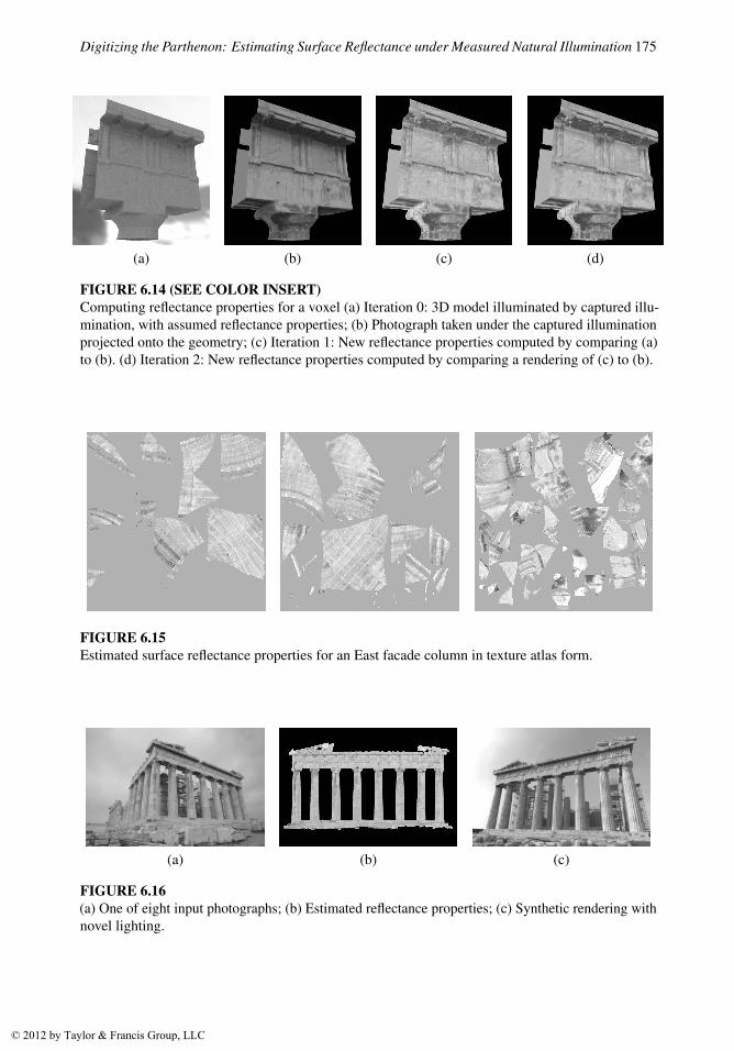
FIGURE 6.15Estimated surface reflectance properties for an East facade column in texture atlas form.

(a) (b) (c)

FIGURE 6.16(a) One of eight input photographs; (b) Estimated reflectance properties; (c) Synthetic rendering withnovel lighting.



6.5 Results

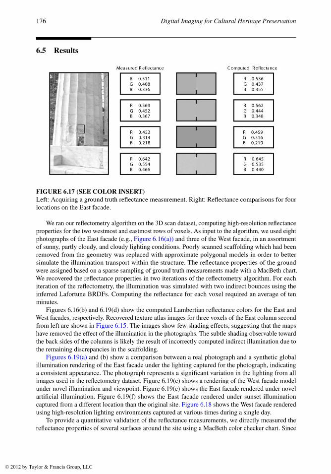
FIGURE 6.17 (SEE COLOR INSERT)Left: Acquiring a ground truth reflectance measurement. Right: Reflectance comparisons for fourlocations on the East facade.

We ran our reflectometry algorithm on the 3D scan dataset, computing high-resolution reflectanceproperties for the two westmost and eastmost rows of voxels. As input to the algorithm, we used eightphotographs of the East facade (e.g., Figure 6.16(a)) and three of the West facade, in an assortmentof sunny, partly cloudy, and cloudy lighting conditions. Poorly scanned scaffolding which had beenremoved from the geometry was replaced with approximate polygonal models in order to bettersimulate the illumination transport within the structure. The reflectance properties of the groundwere assigned based on a sparse sampling of ground truth measurements made with a MacBeth chart.We recovered the reflectance properties in two iterations of the reflectometry algorithm. For eachiteration of the reflectometry, the illumination was simulated with two indirect bounces using theinferred Lafortune BRDFs. Computing the reflectance for each voxel required an average of tenminutes.

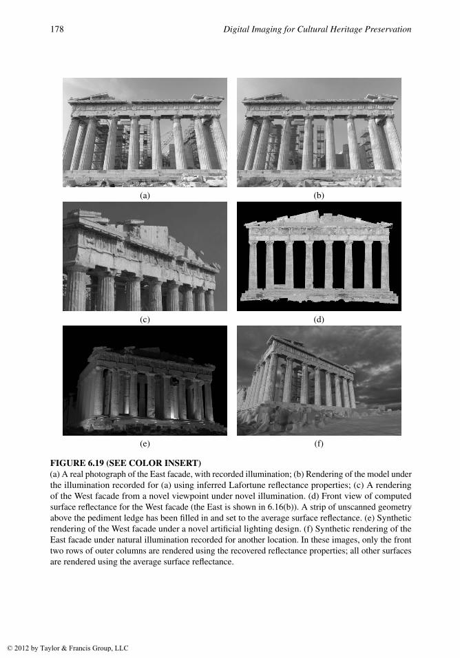
Figures 6.16(b) and 6.19(d) show the computed Lambertian reflectance colors for the East andWest facades, respectively. Recovered texture atlas images for three voxels of the East column secondfrom left are shown in Figure 6.15. The images show few shading effects, suggesting that the mapshave removed the effect of the illumination in the photographs. The subtle shading observable towardthe back sides of the columns is likely the result of incorrectly computed indirect illumination due tothe remaining discrepancies in the scaffolding.

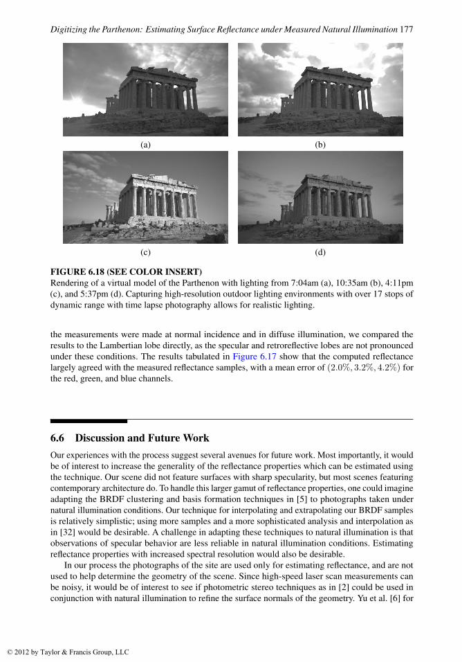
Figures 6.19(a) and (b) show a comparison between a real photograph and a synthetic globalillumination rendering of the East facade under the lighting captured for the photograph, indicatinga consistent appearance. The photograph represents a significant variation in the lighting from allimages used in the reflectometry dataset. Figure 6.19(c) shows a rendering of the West facade modelunder novel illumination and viewpoint. Figure 6.19(e) shows the East facade rendered under novelartificial illumination. Figure 6.19(f) shows the East facade rendered under sunset illuminationcaptured from a different location than the original site. Figure 6.18 shows the West facade renderedusing high-resolution lighting environments captured at various times during a single day.

To provide a quantitative validation of the reflectance measurements, we directly measured thereflectance properties of several surfaces around the site using a MacBeth color checker chart. Since



(a) (b)

(c) (d)

FIGURE 6.18 (SEE COLOR INSERT)Rendering of a virtual model of the Parthenon with lighting from 7:04am (a), 10:35am (b), 4:11pm(c), and 5:37pm (d). Capturing high-resolution outdoor lighting environments with over 17 stops ofdynamic range with time lapse photography allows for realistic lighting.

the measurements were made at normal incidence and in diffuse illumination, we compared theresults to the Lambertian lobe directly, as the specular and retroreflective lobes are not pronouncedunder these conditions. The results tabulated in Figure 6.17 show that the computed reflectancelargely agreed with the measured reflectance samples, with a mean error of (2.0%, 3.2%, 4.2%) forthe red, green, and blue channels.

6.6 Discussion and Future WorkOur experiences with the process suggest several avenues for future work. Most importantly, it wouldbe of interest to increase the generality of the reflectance properties which can be estimated usingthe technique. Our scene did not feature surfaces with sharp specularity, but most scenes featuringcontemporary architecture do. To handle this larger gamut of reflectance properties, one could imagineadapting the BRDF clustering and basis formation techniques in [5] to photographs taken undernatural illumination conditions. Our technique for interpolating and extrapolating our BRDF samplesis relatively simplistic; using more samples and a more sophisticated analysis and interpolation asin [32] would be desirable. A challenge in adapting these techniques to natural illumination is thatobservations of specular behavior are less reliable in natural illumination conditions. Estimatingreflectance properties with increased spectral resolution would also be desirable.

In our process the photographs of the site are used only for estimating reflectance, and are notused to help determine the geometry of the scene. Since high-speed laser scan measurements canbe noisy, it would be of interest to see if photometric stereo techniques as in [2] could be used inconjunction with natural illumination to refine the surface normals of the geometry. Yu et al. [6] for



(a) (b)

(c) (d)

(e) (f)

FIGURE 6.19 (SEE COLOR INSERT)(a) A real photograph of the East facade, with recorded illumination; (b) Rendering of the model underthe illumination recorded for (a) using inferred Lafortune reflectance properties; (c) A renderingof the West facade from a novel viewpoint under novel illumination. (d) Front view of computedsurface reflectance for the West facade (the East is shown in 6.16(b)). A strip of unscanned geometryabove the pediment ledge has been filled in and set to the average surface reflectance. (e) Syntheticrendering of the West facade under a novel artificial lighting design. (f) Synthetic rendering of theEast facade under natural illumination recorded for another location. In these images, only the fronttwo rows of outer columns are rendered using the recovered reflectance properties; all other surfacesare rendered using the average surface reflectance.



example used photometric stereo from different solar positions to estimate surface normals for abuilding’s environment; it seems possible that such estimates could also be made given three imagesof general incident illumination with or without the sun.

Our experience calibrating the illumination measurement device showed that its images could beaffected by sky polarization. We tested the alternative of using an upward-pointing fisheye lens toimage the sky, but found significant polarization sensitivity toward the horizon as well as undesirablelens flare from the sun. More successfully, we used a 91% reflective aluminum-coated hemisphericallens and found it to have less than 5% polarization sensitivity, making it suitable for lighting capture.For future work, it might be of interest to investigate whether sky polarization, explicitly captured,could be leveraged in determining a scene’s specular parameters [45].

Finally, it could be of interest to use this framework to investigate the more difficult problem ofestimating a scene’s reflectance properties under unknown natural illumination conditions. In thiscase, estimation of the illumination could become part of the optimization process, possibly by fittingto a principal component model of measured incident illumination conditions.

6.7 ConclusionWe have presented a process for estimating spatially-varying surface reflectance properties of anoutdoor scene based on scanned 3D geometry, BRDF measurements of representative surface samples,and a set of photographs of the scene under measured natural illumination conditions. Applying theprocess to a real-world archaeological site, we found it able to recover reflectance properties close toground truth measurements, and able to produce renderings of the scene under novel illuminationconsistent with real photographs. The encouraging results suggest further work be carried out tocapture more general reflectance properties of real-world scenes using natural illumination.

AcknowledgmentsThe authors would like to acknowledge the following individuals and organizations which supportedthis project: Richard Lindheim, David Wertheimer, Neil Sullivan, Nikos Toganidis, Katerina Paraschis,Tomas Lochman, Manolis Korres, Angeliki Arvanitis, James Blake, Bri Brownlow, Chris Butler,Elizabeth Cardman, Alan Chalmers, Paolo Cignoni, Yikuong Chen, Jon Cohen, Costis Dallas, ChristaDeacy-Quinn, Paul T. Debevec, Naomi Dennis, Apostolos Dimopoulos, George Drettakis, Paul EgriCosta-Gavras, Darin Grant, Rob Groome, Christian Guillon, Craig Halperin, Youda He, Eric Hoffman,Leslie Ikemoto, Peter James, David Jillings, Genichi Kawada, Shivani Khanna, Randal Kleiser, CathyKominos, Jim Korris, Marc Levoy, Dell Lunceford, Donat-Pierre Luigi, Mike Macedonia, BrianManson, Paul Marty, Hiroyuki Matsuguma, David Miraglia, Chris Nichols, Chrysostomos Nikias,Mark Ollila, Yannis Papoutsakis, John Parmentola, Fred Persi, Dimitrios Raptis, Simon Ratcliffe,Mark Sagar, Roberto Scopigno, Alexander Singer, Judy Singer, Diane Suzuki, Laurie Swanson, BillSwartout, Despoina Theodorou, Mark Timpson, Rippling Tsou, Zach Turner, Esdras Varagnolo,Greg Ward, Karen Williams, Min Yu and The Work Site of the Acropolis, The Louvre, The BaselSkulpturhalle, The British Museum, The Spurlock Museum, The Herodion Hotel, QuantapointInc., Geometry Systems Inc., CNR Pisa, Alia, The US Army, TOPPAN Printing Co Ltd., and TheUniversity of Southern California.



Bibliography[1] M. Levoy, K. Pulli, B. Curless, S. Rusinkiewicz, D. Koller, L. Pereira, M. Ginzton, S. Anderson,

J. Davis, J. Ginsberg, J. Shade, and D. Fulk, “The Digital Michelangelo Project: 3D Scanningof Large Statues,” Proceedings of SIGGRAPH 2000, pp. 131–144, July 2000.

[2] H. Rushmeier, F. Bernardini, J. Mittleman, and G. Taubin, “Acquiring Input for Rendering atAppropriate Levels of Detail: Digitizing a Pieta,” Eurographics Rendering Workshop 1998,pp. 81–92, June 1998.

[3] K. Ikeuchi, “Modeling from Reality,” in Proceedings Third International Conference on 3-DDigital Imaging and Modeling (Quebec City), pp. 117–124, May 2001.

[4] S. Marschner, Inverse Rendering for Computer Graphics. PhD thesis, Cornell University,August 1998.

[5] H. P. A. Lensch, J. Kautz, M. Goesele, W. Heidrich, and H.-P. Seidel, “Image-Based Recon-struction of Spatial Appearance and Geometric Detail,” ACM Transactions on Graphics, vol. 22,pp. 234–257, Apr. 2003.

[6] Y. Yu and J. Malik, “Recovering Photometric Properties of Architectural Scenes from Pho-tographs,” in Proceedings of SIGGRAPH 98, Computer Graphics Proceedings, Annual Confer-ence Series, pp. 207–218, July 1998.

[7] Y. Yu, P. Debevec, J. Malik, and T. Hawkins, “Inverse Global Illumination: Recovering Re-flectance Models of Real Scenes from Photographs,” Proceedings of SIGGRAPH 99, pp. 215–224, August 1999.

[8] P. Debevec, C. Tchou, A. Gardner, T. Hawkins, C. Poullis, J. Stumpfel, A. Jones, N. Yun,P. Einarsson, T. Lundgren, M. Fajardo, P. Martinez, “Estimating Surface Reflectance Propertiesof a Complex Scene under Captured Natural Illumination,” Technical report, USC, 2004.ICT-TR-06.2004.

[9] P. Besl and N. McKay, “A Method for Registration of 3-d Shapes,” IEEE Transactions onPattern Analysis and Machine Intelligence, vol. 14, pp. 239–256, 1992.

[10] Y. Chen and G. Medioni, “Object Modeling from Multiple Range Images,” Image and VisionComputing, vol. 10, pp. 145–155, April 1992.

[11] G. Turk and M. Levoy, “Zippered Polygon Meshes from Range Images,” in Proceedings ofSIGGRAPH 94, Computer Graphics Proceedings, Annual Conference Series (Orlando, Florida),pp. 311–318, ACM SIGGRAPH / ACM Press, July 1994. ISBN 0-89791-667-0.

[12] B. Curless and M. Levoy, “A Volumetric Method for Building Complex Models from Range Im-ages,” in Proceedings of SIGGRAPH 96, Computer Graphics Proceedings, Annual ConferenceSeries (New Orleans, Louisiana), pp. 303–312, ACM SIGGRAPH / Addison Wesley, August1996.

[13] G. J. W. Larson, “Measuring and Modeling Anisotropic Reflection,” in Computer Graphics(Proceedings of SIGGRAPH 92), vol. 26 (Chicago, Illinois), pp. 265–272, July 1992.

[14] M. Oren and S. K. Nayar, “Generalization of Lambert’s Reflectance Model,” Proceedings ofSIGGRAPH 94, pp. 239–246, July 1994.



[15] E. P. F. Lafortune, S.-C. Foo, K. E. Torrance, and D. P. Greenberg, “Non-Linear Approximationof Reflectance Functions,” Proceedings of SIGGRAPH 97, pp. 117–126, 1997.

[16] F. E. Nicodemus, J. C. Richmond, J. J. Hsia, I. W. Ginsberg, and T. Limperis, “GeometricConsiderations and Nomenclature for Reflectance,” National Bureau of Standards Monograph160, October 1977.

[17] S. R. Marschner, S. H. Westin, E. P. F. Lafortune, K. E. Torrance, and D. P. Greenberg, “Image-Based BRDF Measurement Including Human Skin,” Eurographics Rendering Workshop 1999,June 1999.

[18] H. W. Jensen, S. R. Marschner, M. Levoy, and P. Hanrahan, “A Practical Model for SubsurfaceLight Transport,” in Proceedings of SIGGRAPH 2001, Computer Graphics Proceedings, AnnualConference Series, pp. 511–518, ACM Press/ACM SIGGRAPH, August 2001. ISBN 1-58113-292-1.

[19] S. R. Marschner and D. P. Greenberg, “Inverse Lighting for Photography,” in Proceedings ofthe IS&T/SID Fifth Color Imaging Conference, November 1997.

[20] I. Sato, Y. Sato, and K. Ikeuchi, “Ilumination Distribution from Shadows,” in Proceedings ofIEEE Conference on Computer Vision and Pattern Recognition (CVPR’99), pp. 306–312, June1999.

[21] P. Debevec, “Rendering Synthetic Objects into Real Scenes: Bridging Traditional and Image-Based Graphics with Global Illumination and High Dynamic Range Photography,” in Pro-ceedings of SIGGRAPH 98, Computer Graphics Proceedings, Annual Conference Series,pp. 189–198, July 1998.

[22] P. E. Debevec and J. Malik, “Recovering High Dynamic Range Radiance Maps from Pho-tographs,” in Proceedings of SIGGRAPH 97, Computer Graphics Proceedings, Annual Confer-ence Series, pp. 369–378, Aug. 1997.

[23] Y. Sato, M. D. Wheeler, and K. Ikeuchi, “Object Shape and Reflectance Modeling fromObservation,” in SIGGRAPH 97, pp. 379–387, 1997.

[24] K. Ikeuchi and B. Horn, “An Application of the Photometric Stereo Method,” in 6th Interna-tional Joint Conference on Artificial Intelligence (Tokyo, Japan), pp. 413–415, August 1979.

[25] S. K. Nayar, K. Ikeuchi, and T. Kanade, “Determining Shape and Reflectance of HybridSurfaces by Photometric Sampling,” IEEE Transactions on Robotics and Automation, vol. 6,pp. 418–431, August 1994.

[26] C. Rocchini, P. Cignoni, C. Montani, and R. Scopigno, “Acquiring, Stitching and BlendingDiffuse Appearance Attributes on 3D Models,” The Visual Computer, vol. 18, no. 3, pp. 186–204, 2002.

[27] P. Debevec, T. Hawkins, C. Tchou, H.-P. Duiker, W. Sarokin, and M. Sagar, “Acquiring theReflectance Field of a Human Face,” Proceedings of SIGGRAPH 2000, pp. 145–156, July 2000.

[28] C. Loscos, M.-C. Frasson, G. Drettakis, B. Walter, X. Granier, and P. Poulin, “Interactive VirtualRelighting and Remodeling of Real Scenes,” in Eurographics Rendering Workshop 1999, June1999.

[29] S. Boivin and A. Gagalowicz, “Inverse Rendering from a Single Image,” in Proceedings ofIS&T Color in Graphics, Imaging, and Vision, 2002.



[30] J.-Y. Bouguet, “Camera Calibration Toolbox for Matlab,” 2002.http://www.vision.caltech.edu/bouguetj/calib doc/.

[31] Z. Zhang, “A Flexible New Technique for Camera Calibration,” IEEE Transactions on PatternAnalysis and Machine Intelligence, vol. 22, no. 11, pp. 1330–1334, 2000.

[32] W. Matusik, H. Pfister, M. Brand, and L. McMillan, “A Data-Driven Reflectance Model,” ACMTransactions on Graphics, vol. 22, pp. 759–769, July 2003.

[33] V. Masselus, P. Dutre, and F. Anrys, “The Free-Form Light Stage,” in Rendering Techniques2002: 13th Eurographics Workshop on Rendering, pp. 247–256, June 2002.

[34] S. Marschner, B. Guenter, and S. Raghupathy, “Modeling and Rendering for Realistic Fa-cial Animation,” in Rendering Techniques 2000: 11th Eurographics Workshop on Rendering,pp. 231–242, June 2000.

[35] G. S. Miller and C. R. Hoffman, “Illumination and Reflection Maps: Simulated Objects inSimulated and Real Environments,” in SIGGRAPH 84 Course Notes for Advanced ComputerGraphics Animation, July 1984.

[36] J. Hancock, D. Langer, M. Hebert, R. Sullivan, D. Ingimarson, E. Hoffman, M. Mettenleiter,and C. Froehlich, “Active Laser Radar for High-Performance Measurements,” in ProceedingsIEEE International Conference on Robotics and Automation (Leuven, Belgium), May 1998.

[37] M. Callieri, P. Cignoni, F. Ganovelli, C. Montani, P. Pingi, and R. Scopigno, “VCLAB’s Toolsfor 3D Range Data Processing,” in VAST 2003 and Eurographics Symposium on Graphics andCultural Heritage, 2003.

[38] Graphite, 2003. http://www.loria.fr/ levy/Graphite/index.html.

[39] B. Levy, S. Petitjean, N. Ray, and J. Maillot, “Least Squares Conformal Maps for AutomaticTexture Atlas Generation,” ACM Transactions on Graphics, vol. 21, pp. 362–371, July 2002.

[40] QSlim, 1999. http://graphics.cs.uiuc.edu/ garland/software/qslim.html.

[41] M. Garland and P. S. Heckbert, “Simplifying Surfaces with Color and Texture Using QuadricError Metrics,” in IEEE Visualization ’98, pp. 263–270, Oct. 1998.

[42] H. P. A. Lensch, W. Heidrich, and H.-P. Seidel, “A Silhouette-Based Algorithm for TextureRegistration and Stitching,” Graphical Models, vol. 63, pp. 245–262, Apr. 2001.

[43] C. Buehler, M. Bosse, L. McMillan, S. J. Gortler, and M. F. Cohen, “Unstructured LumigraphRendering,” in Proceedings of ACM SIGGRAPH 2001, Computer Graphics Proceedings, AnnualConference Series, pp. 425–432, Aug. 2001.

[44] J. Kajiya, “The Rendering Equation,” in SIGGRAPH 86, pp. 143–150, 1986.

[45] S. Nayar, X. Fang, and T. Boult, “Separation of Reflection Components Using Color andPolarization,” International Journal of Computer Vision, vol. 21, pp. 163–186, February 1997.


http://www.vision.caltech.edu

http://www.loria.fr/

http://graphics.cs.uiuc.edu/

Digitizing the Parthenon: Estimating Surface Reﬂectance ...ict.usc.edu/pubs/Digitizing the...

Documents

Transcript of Digitizing the Parthenon: Estimating Surface Reﬂectance ...ict.usc.edu/pubs/Digitizing the...