DIGITAL SURFACE MODELS FROM ULTRACAM-X IMAGES

M. Gruber , S. Schneider

Microsoft Photogrammetry, Anzengrubergasse 8, A-8010 Graz - (michgrub, susannes)@microsoft.com

KEY WORDS: UltraCamX, Digital Surface Models, Digital Images, Large Scale Mapping, Aerial Images ABSTRACT: UltraCamX is the newest large format digital aerial camera system by Microsoft Photogrammetry (former Vexcel) and was introduced in 2006. We present a short technical overview about the sensor and we show results from a data experiment. Images from this sensor were produced at high overlaps and used to create digital surface models. In this paper the geometric accuracy of the digital surface data and the quality of UltraCamX images are presented. UltraCamX offers to capture one frame at an interval of 1.35 seconds. This allows to producing images at high overlaps at large scale and reasonable speed of the aircraft. For the data experiment a ground sampling distance of 10cm was produced at a forward overlap of 90%. Such redundant image data can be used to improve automation and robustness during the processing of dense surface models.

1.1 1. INTRODUCTION

Overlapping images are one important source data set for three dimensional object reconstruction and surface modeling. This application - known as “shape from stereo” – does rely on the quality of the source images. Geometric accuracy and radiometric bandwidth are the two most important requirements which are requested in order to produce quality results. Since a few years large format digital aerial cameras are available and did find their way into the photogrammetric production. It was very obvious that the digital sensor did show advantages over film based, scanned images. The most important advantage can be seen in the radiometric quality, thus no longer film grain noise affects the matching process. Another advantage of digital sensors can be seen in the new all digital workflow excluding the expensive and time consuming handling of the film. Digital image data can be produced and stored at very attractive costs. Therefore the acquisition of data capture may be reorganized. Not the minimum of images but redundancy and robustness are the requirements of the all digital photogrammetric projects. The new digital sensor system by Microsoft, the UltraCam X was used to capture images over a well known project area. Digital surface information was extracted from UltraCamX images by means of image analysis. The project area of Gleisdorf was mapped at a ground sampling distance (GSD) of 10 cm at a special flight pattern of high overlap. 9 lines are flown in N-S direction, with each about 31 images and 5 lines in the E-W direction, with about 25 images. The project is flown with 80 % forward overlap and 65% side overlap. We present the quality of the resulting Digital Surface Model (DSM) datasets. From one test flight one DSM was derived from the North to South flight lines and one from the East to West flight lines. The resulting DSMs are compared with Ground Control Points (GCP) in the area and z-Differences are shown.

UltraCam X

The UltraCam X large format digital aerial camera system was introduced in 2006 and can be seen as the successor of Vexcel’s UltraCam D. The basic concept of the design did not change. The sensor unit consists of eight camera heads. Four camera heads are responsible for the large format panchromatic image, another set of four camera heads contribute with four color bands in red, green, blue and near infrared. The sensor produces images of 14430 by 9420 pixels at a frame rate of 1 frame in 1.35 seconds. Thus high overlaps of 80 % along track can be achieved at 5 cm GSD and a reasonable speed of the aircraft. The physical dimension of the image is 103.9 mm by 67.8 mm at a Pixel size of 7.2 µm. The principal distance of the camera is 100.5 mm.

Fig.1: UltraCam X digital aerial camera system with the Sensor Unit (right) and the airborne Computing Unit including two

removable Data Units (left). The data storage system of the camera offers storage space for almost 4700 frames, thus the system is well prepared for intensive image harvest at large scales and at high overlaps. All image data are initially stored at 16 bit bandwidth (see Fig. 1).

In: Stilla U et al (Eds) PIA07. International Archives of Photogrammetry, Remote Sensing and Spatial Information Sciences, 36 (3/W49B)¯¯¯¯¯¯¯¯¯¯¯¯¯¯¯¯¯¯¯¯¯¯¯¯¯¯¯¯¯¯¯¯¯¯¯¯¯¯¯¯¯¯¯¯¯¯¯¯¯¯¯¯¯¯¯¯¯¯¯¯¯¯¯¯¯¯¯¯¯¯¯¯¯¯¯¯¯¯¯¯¯¯¯¯¯¯¯¯¯¯¯¯¯¯¯¯¯¯¯¯¯¯¯¯¯¯¯¯¯

47

1.2 Basic source data

During the routine delivery process every UltraCamX camera systems has to pass a specific test flight which is performed over the test field of Gleisdorf near Graz. Figure 2 shows an overview of the flight plan for that area. The size of the Gleisdorf test field is about 5 km by 7 km. It shows a huge diversity of cultivation including build up areas, traffic infrastructure, agricultural plans and forests. The ground truth consists of 56 full ground control points and a local GPS station. The source data sets for our DSM quality assessment consist of images taken at a ground sampling distance of 10 cm at a flying height of 1400 m above ground level. The forward overlap was set to 80% the side lap was set to 65% resulting into a distance between flight lines of 500 m and a base length of 200 m. This special flight pattern supports redundancy and thus automatic blunder detection. Flight lines facing north to south and flight lines facing east to west were used to produce two different sets of DSMs. During the flight mission GPS/IMU information was collected.

Fig. 2: Overview of the Gleisdorf area with flight lines in two directions and 500 m spacing. The base distance between photo centers is 200 m.

The DSM area is marked up by the blue quadrangle. The size of the source images of the UltraCamX camera system is 14430 pixels cross track and 9420 pixel along track, thus a footprint of 1443 m by 942 m is covered by one frame at a flying height of 1400 m. The single base distance between two images is 200 m, thus the resulting base to height ratio is only 1/7. Therefore a set of three or more images is used for every point measurement. This leads to a base to height ratio of 1/3.5, 1/2.3 or even 1/1.75 and increases the vertical quality and the robustness of the set. Fig. 3 shows one single frame of the camera system. The sub area on the right gives an impression of the level of detail and the radiometric quality of the image. The flight mission took place on May, 10th of 2007.

Fig. 3: Source image from UltraCamX at a format of 14430 by 9420 pixels. The entire frame is shown on the left, the detail on the right

covers a footprint of 68 by 90 meter. 1.3 The workflow

The entire photogrammetric process consists of the three basic steps of source data acquisition including the post-processing of the raw image data, geo referencing of the images based on GPS/IMU supported aerial triangulation and DSM computation by means of dense image matching. The post processing is done by the camera specific software package OPC (Office Processing Center) and converts the set of 13 raw sub images of each frame into one single large format panchromatic image and one four band color image. This process includes the so-called stitching between overlapping sub images and also introduces the parameters of the laboratory calibration data set. Such post processed and therefore geometrically and radiometrically corrected images are then introduced into the aero triangulation. The automatic aerotriangulation (AAT) is performed by using the Match AT software product from INPHO GmbH, Stuttgart, Germany. A camera specific bundle adjustment is then added by using the BINGO software product from GIP, Aalen, Germany. The GPS and IMU processing was supported by IGI mbH, Kreuztal, Germany. After the images are geo referenced a refined AT is computed and matching points are extracted. These procedures give additional information on the accuracy of the AT, used for the DSM computation in the next step. The DSM algorithm was especially developed for processing UltraCam images. A hybrid multi-view matching algorithm is used for calculating height field images. In a first stage a coarse matching and a dense matching is done to create overlapping range images. In a second stage those overlapping images are fused to non-overlapping height field images which result in the final DSM. Fig. 4 shows the resulting DSM of the central Gleisdorf area. Within this area six small samples were chosen to investigate the quality of the digital surface models. The positions of these samples are marked up in Fig. 4.

PIA07 - Photogrammetric Image Analysis --- Munich, Germany, September 19-21, 2007¯¯¯¯¯¯¯¯¯¯¯¯¯¯¯¯¯¯¯¯¯¯¯¯¯¯¯¯¯¯¯¯¯¯¯¯¯¯¯¯¯¯¯¯¯¯¯¯¯¯¯¯¯¯¯¯¯¯¯¯¯¯¯¯¯¯¯¯¯¯¯¯¯¯¯¯¯¯¯¯¯¯¯¯¯¯¯¯¯¯¯¯¯¯¯¯¯¯¯¯¯¯¯¯¯¯¯¯¯

48

2.2

Fig. 4: DSM of the central Gleisdorf area including the six samples for detailed analysis.

2. DETAILED ANALYSIS AND RESULTS

The following analysis is performed in order to investigate the accuracy of the entire photogrammetric process and the resulting DSM data sets. The first quality measure of the process can be given from aerial triangulation. Then we compare the DSM data derived from the two sets of images taken under the different flying direction North to South vs. East to West (NS data set and EW data set). All available image data from the flight missions show a GSD of 10 cm. The DSM datasets were processed at a mesh size of 20 cm, thus the DSM grid spacing corresponds to two pixels of the source images. Matlab (The MathWorks, Inc.) was used to compute the specific test data and the height profiles. The overlay of checkpoints and DSM was performed in ESRI ArcGIS. 2.1 Aerotriangulation results

The aerotriangulation process includes the automatic tie point matching based on a manifold of up to 15 images for each of the two data sets, the manual measurement of ground control points in the images and the adjustment of the redundant set of observations by means of the least squares method. This process was done by using the MatchAT software product. In addition to this a camera specific set of auto calibration parameters was introduced and estimated by using the BINGO software package. The small image distortions which were computed during the auto calibration were then introduced into the image post processing and therefore the geometric image quality and the DSM computation could be improved. Sensor Project Accuracy GSD HAGL Sigma_o Rmse z (cm) (m) (µm) (m) UCX 10 1400 0.80 0.035

Table 1. Overview of the main AT parameters and results. The good vertical accuracy corresponds to relative accuracy of 1/40 000.

Comparing the DSM datasets against ground truth

The initial test of the geometric quality of the DSM data was performed by comparing DSM data vs. ground truth. For this test a subset of 16 GCPs of the Gleisdorf area was selected and back projected into the DSM data sets. The vertical value of the DSM mesh near to the specific GCP was then extracted and compared against the z coordinate of the GCP. The results correspond to the expectations from the good results of the aerial triangulation. The standard deviation of the 16 height differences (13 differences in the case of data set NS) was in the range of 1 pixel (~ 10 cm).

PN Z GCP Z NS zDiff NS Z EW zDiff EWP 1 352.688 352.510 0.178 352.518 0.170

P 2 367.966 367.823 0.143 367.843 0.123

P 3 361.062 361.032 0.030 361.002 0.060

P 4 384.855 384.771 0.084 384.702 0.153

P 5 373.465 - - 373.490 -0.025

P 6 359.916 359.889 0.027 359.884 0.032

P 7 349.424 349.423 0.001 349.389 0.035

P 8 348.021 348.001 0.020 347.896 0.125

P 9a 352.230 352.097 0.133 352.140 0.090

P 9b 352.594 352.656 -0.062 352.532 0.062

P 10 348.227 348.248 -0.021 348.233 -0.006

P 11 364.108 - - 364.125 -0.017

P 12 360.394 - - 360.509 -0.115

P 13 344.379 344.457 -0.078 344.380 -0.001

P 14 342.803 342.938 -0.135 342.956 -0.153

P 15 345.585 345.837 -0.252 345.751 -0.166

MIN -0.252 -0.166

MAX 0.178 0.170

Mean 0.005 0.023

Stdev ±0.119 ± 0.102

Table 2. Comparison of z-Values of two different DSM datasets against check points of the Gleisdorf area (all data given in meter).

Table 2 lists all GCPs with their given z-values (Z GCP) and the corresponding z-Values extracted from the two DSM datasets (Z NS and Z EW). The two additional columns show the differences between Z GCP and z-values from the DSM (z Diff NS and z Diff EW). Finally Table 2 presents minimum and maximum value, mean value and standard deviation which were computed from the set of vertical differences. The relative accuracy in z corresponds to 1/12000 for data set NS and 1/14000 for data set EW. The location of the 16 GCPs is shown in Fig. 5. Comparing the z-values of the two DSM data sets at the 13 positions of the common GCPs we computed a mean difference of 0.035 m (1/3 of a pixel) and a standard deviation of 0.064 m. Interpreting the mean difference as a global offset we reduced this value from each height difference. The standard deviation of that set of 13 values was then only 0.053 m which is about 1/2 of a pixel of the source images.

In: Stilla U et al (Eds) PIA07. International Archives of Photogrammetry, Remote Sensing and Spatial Information Sciences, 36 (3/W49B)¯¯¯¯¯¯¯¯¯¯¯¯¯¯¯¯¯¯¯¯¯¯¯¯¯¯¯¯¯¯¯¯¯¯¯¯¯¯¯¯¯¯¯¯¯¯¯¯¯¯¯¯¯¯¯¯¯¯¯¯¯¯¯¯¯¯¯¯¯¯¯¯¯¯¯¯¯¯¯¯¯¯¯¯¯¯¯¯¯¯¯¯¯¯¯¯¯¯¯¯¯¯¯¯¯¯¯¯¯

49

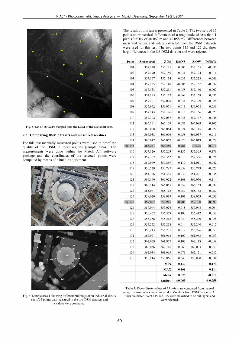
Fig. 5: Set of 16 GCPs mapped onto the DSM of the Gleisdorf area. 2.3 Comparing DSM datasets and measured z-values

For this test manually measured points were used to proof the quality of the DSM in local regions (sample areas). The measurements were done within the Match AT software package and the coordinates of the selected points were computed by means of a bundle adjustment.

Fig. 6: Sample area 1 showing different buildings of an industrial site. A

set of 35 points was measured in the two DSM datasets and z values were compared.

The result of this test is presented in Table 3. The two sets of 35 points show vertical differences of a magnitude of less than 1 pixel (StdDev of ±0.069 m and ±0.058 m). Differences between measured values and values extracted from the DSM data sets were used for this test. The two points 115 and 125 did show larg differences in the NS DSM data set and were rejected.

Table 3: Z-coordinate values of 35 points are computed from manual

image measurements and compared to Z-values from DSM data sets. All units are meter. Point 115 and 125 were classified to be out layers and

were rejected.

Point Zmeasured Z NS DiffNS Z OW DiffOW

101 357,128 357,125 0,003 357,165 -0,037

102 357,190 357,159 0,031 357,174 0,016

103 357,167 357,134 0,033 357,213 -0,046

104 357,135 357,140 -0,005 357,167 -0,032

105 357,153 357,211 -0,058 357,160 -0,007

106 357,195 357,127 0,068 357,158 0,037

107 357,101 357,070 0,031 357,129 -0,028

108 356,962 356,951 0,011 356,998 -0,036

109 357,143 357,126 0,017 357,166 -0,023

110 357,102 357,057 0,045 357,147 -0,045

111 366,191 366,109 0,082 366,089 0,102

112 366,088 366,064 0,024 366,115 -0,027

113 366,038 366,096 -0,058 366,057 -0,019

114 366,047 366,067 -0,020 366,019 0,028

rej. 115 365,231 364,450 0,781 365,25 -0,019

116 357,126 357,263 -0,137 357,305 -0,179

117 357,362 357,352 0,010 357,336 0,026

118 350,969 350,859 0,110 351,011 -0,042

119 350,729 350,787 -0,058 350,749 -0,020

120 351,326 351,365 -0,039 351,291 0,035

121 366,190 366,022 0,168 366,076 0,114

122 366,114 366,055 0,059 366,153 -0,039

123 365,061 365,118 -0,057 365,148 -0,087

124 359,020 358,919 0,101 359,053 -0,033

rej. 125 359,007 359,915 -0,908 359,100 -0,093

126 359,044 359,026 0,018 359,048 -0,004

127 356,462 356,359 0,103 356,412 0,050

128 355,258 355,218 0,040 355,230 0,028

129 355,252 355,238 0,014 355,240 0,012

130 355,243 355,231 0,012 355,296 -0,053

131 362,021 361,912 0,109 361,968 0,053

132 362,059 361,957 0,102 362,118 -0,059

133 362,056 362,116 -0,060 362,003 0,053

134 362,034 361,963 0,071 362,121 -0,087

135 350,914 350,866 0,048 350,880 0,034

MIN -0.137 -0.179

MAX 0.168 0.114

Mean 0.025 -0.010

StdDev ±0.069 ± 0.058

PIA07 - Photogrammetric Image Analysis --- Munich, Germany, September 19-21, 2007¯¯¯¯¯¯¯¯¯¯¯¯¯¯¯¯¯¯¯¯¯¯¯¯¯¯¯¯¯¯¯¯¯¯¯¯¯¯¯¯¯¯¯¯¯¯¯¯¯¯¯¯¯¯¯¯¯¯¯¯¯¯¯¯¯¯¯¯¯¯¯¯¯¯¯¯¯¯¯¯¯¯¯¯¯¯¯¯¯¯¯¯¯¯¯¯¯¯¯¯¯¯¯¯¯¯¯¯¯

50

2.4 Comparing DSM datasets computed from different sets of aerial images (flying directions NS vs. EW)

In the following section we show the vertical differences of six sample areas (cf. Fig. 4) computed from the two DSM data sets. Each sample area consists of 1 000 000 height values, the size of each area is 200 m by 200 m. Each area has a specific kind of cultivation. Sample area 1 consists of industrial buildings with flat roofs, area 2 consists of residential buildings in the center of the village of Gleisdorf including the gothic style church, area 5 includes parts of a motor highway and area 3, 4 and 6 are a mixture of agricultural flat land and forest areas.

Fig. 7: Sample area 1 to 6 and the height differences computed from the

two DSM data sets. Height differences are coded by different grey levels representing 5 classes of magnitude.

Sample |Dz| < 0.3 m |Dz| < 0.2 m |Dz| < 0.1 m

1 86.4 % 74.9 % 45.8 % 2 81.6 % 70.0 % 43.4 % 3 84.2 % 74.2 % 50.0 % 4 96.1 % 93.2 % 73.1 % 5 85.1 % 76.5 % 49.9 % 6 97.7 % 91.7 % 60.9 %

1 to 6 88.5 % 80.1 % 53.9 %

Table 4: Vertical differences within each sample area are mapped into three classes. The classes represent maximum height differences

of 0.3 m, 0.2 m and 0.1 m.

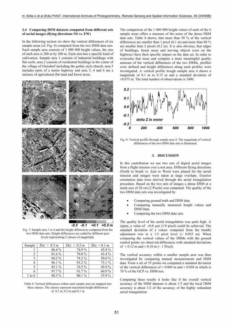
The comparison of the 1 000 000 height values of each of the 6 sample areas offers a measure of the noise of the dense DSM data sets. Table 4 shows, that more than 50 % of the vertical differences are smaller than 1 pixel (0.1 m) and more than 80 % are smaller than 2 pixels (0.2 m). It is also obvious, that edges of buildings, forest areas and moving objects (cars on the highway) have their specific impact on the data set. In order to overcome that issue and compute a more meaningful quality measure of the vertical differences of the two DSMs, profiles were defined and height differences along such profiles were investigated. A vertical profile trough sample area 4 shows a magnitude of 0.1 m to 0.15 m and a standard deviation of ±0.075 m. The total number of observations is 1000.

Fig. 8: Vertical profile through sample area 4. The magnitude of vertical

differences of the two DSM data sets is illustrated.

3. DISCUSSION

In this contribution we use two sets of digital aerial images from a flight mission over a test area. Different flying directions (North to South vs. East to West) were planed for the aerial mission and images were taken at large overlaps. Exterior orientation data were derived through the aerial triangulation procedure. Based on the two sets of images a dense DSM at a mesh size of 20 cm (2 Pixels) was computed. The quality of the two DSM data sets was investigated by

• Comparing ground truth and DSM data • Comparing manually measured height values and

DSM Data • Comparing the two DSM data sets.

The quality level of the aerial triangulation was quite high. A sigma_o value of ±0.8 µm (1/9 pixel) could be achieved. The standard deviation of z values computed from the bundle adjustment was at a 1/3 pixel level (± 0.035 m). When comparing the vertical values of the DSMs with the ground control points we observed differences with standard deviations of ± 0.12 m and ± 0.10 m (~ 1 Pixel). The vertical accuracy within a smaller sample area was then investigated by comparing manual measurements and DSM data. From a set of 35 points we computed a standard deviation of the vertical differences of ± 0.069 m and ± 0.058 m which is 70 % of the GCP vs. DSM test. Comparing these results it looks like if the overall vertical accuracy of the DSM datasets is about 1/3 and the local DSM accuracy is about 1/2 of the accuracy of the highly redundant aerial triangulation

In: Stilla U et al (Eds) PIA07. International Archives of Photogrammetry, Remote Sensing and Spatial Information Sciences, 36 (3/W49B)¯¯¯¯¯¯¯¯¯¯¯¯¯¯¯¯¯¯¯¯¯¯¯¯¯¯¯¯¯¯¯¯¯¯¯¯¯¯¯¯¯¯¯¯¯¯¯¯¯¯¯¯¯¯¯¯¯¯¯¯¯¯¯¯¯¯¯¯¯¯¯¯¯¯¯¯¯¯¯¯¯¯¯¯¯¯¯¯¯¯¯¯¯¯¯¯¯¯¯¯¯¯¯¯¯¯¯¯¯

51

In addition to the point to point tests of the digital surface models we have compared the two DSMs through six selected sample areas and observed larger variations in the resulting quality measures. Depending on the kind of cultivation or vegetation we observed about 50% of the height differences less than 0.1 m, 80% less than 0.2 m and almost 90% less than 0.3 m. Problems raised with any kind of larger or smaller forest areas as well as buildings and other man made objects with discontinuities of the digital surface. Such discontinuities caused differences in z not as an indicator for inaccurate height measurements but more for a lack of coincidence of the horizontal positions of the discontinuity in the two DSM data sets. However, these effects have been ignored during our tests.

4. FUTURE WORK

The overall accuracy of the DSM data computed automatically from UltraCam images is very promising. Even if space for improvement is still there we see that such data have a value within several applications like digital ortho image production or 3D object reconstruction. Figure 9 gives a small insight view on how such orthophotos can look like. The resulting ortho image sample has a GSD of 10 cm and was produced on top of the DSM at 20 cm mesh size. The sample was processed completely automatically without any manual interaction.

Fig. 9: Samples of a automatically processed orthoimage of the central area of Gleisdorf.

Beyond the ortho image production the dense DSM data is the basic dataset for any three dimensional city modeling task as the Virtual Earth Initiative of Microsoft. About 100 US-cities extracted from UltraCam aerial images are already online on Virtual Earth. One example among many others is the city of Philadelphia (cf. Fig. 10).

Fig. 10: 3D model of the city of Philadelphia, automatically computed from UltraCam images at high overlap.

The three dimensional digital model of the city was extracted automatically from UltraCam images, the single source for geometry and photo texture. The images were taken at high overlap, enabling automatic, redundant and robust processing.

REFERENCES

Gruber M., Franz Leberl, Roland Perko (2003) Paradigmenwechsel in der Photogrammetrie durch Digitale Luftbildaufnahme? Photogrammetrie, Fernerkundung, Geoinformation, Wien 2003. Kremer J., Gruber M. (2004): Operation of The Ultracamd Together with CCNS4/Aerocontrol – First Experiences and Results. The International Archives of Photogrammetry and Remote Sensing, VOL XXXV/1, p. 172 ff., July 2004, Istanbul, Turkey. Leberl F., M. Gruber, M. Ponticelli, S. Bernoegger, R. Perko (2003) The UltraCam Large Format Aerial Digital Camera System. Proceedings of the ASPRS Annual Convention, Anchorage USA, 5-9 May 2003. Zebedin, L. , A. Klaus, B. Gruber-Geymayer, K. Karner (2006) Towards 3D map generation from digital aerial images. International Journal of Photogrammetry and Remote Sensing, Volume 60, p 413ff, 2006.

PIA07 - Photogrammetric Image Analysis --- Munich, Germany, September 19-21, 2007¯¯¯¯¯¯¯¯¯¯¯¯¯¯¯¯¯¯¯¯¯¯¯¯¯¯¯¯¯¯¯¯¯¯¯¯¯¯¯¯¯¯¯¯¯¯¯¯¯¯¯¯¯¯¯¯¯¯¯¯¯¯¯¯¯¯¯¯¯¯¯¯¯¯¯¯¯¯¯¯¯¯¯¯¯¯¯¯¯¯¯¯¯¯¯¯¯¯¯¯¯¯¯¯¯¯¯¯¯

52