Digital signal processing:theoretical background - … Bound...Philips Tech.Rev.42,No. 4,110-144,...
34
Philips Tech. Rev. 42, No. 4,110-144, Dec. 1985 III Digital signal processing: theoretical background A. W. M. van den Enden and N. A. M. Verhoeckx INTRODUCTION Signals exist in many and various forms, ranging from drum signals in the bush to the stop signal from the traffic policeman or the combined radio/television signal received through a central antenna system. The typical common characteristic of all these signals is that they represent a message, or information. The message does not depend greatly on the nature of the signal. The acoustic drum signal can be converted by a microphone into an electrical signal for transmis- sion to the other end of the world. There it can be con- verted into an optical signal for recording on a Com- pact Disc. Then the opposite route can be followed, from optical signal via electrical signal to acoustic sig- nal, without any degradation of the original drum message. In the present state of the technology, electrical sig- nals offer the widest scope for transmission, storage and manipulation ('signal processing'). In signal trans- mission, however, the arrival of the fibre-optic cable has considerably increased the significanee of optical signals. In theoretical considerations the physical nature of a signal is irrelevant. Every signal is 'ab- stracted' to a function of one or more independent variables, representing for example time or position in space. In this article we shall confine ourselves to signals that can be represented as a function of a single vari- able, which we generally take to be 'time', while the value of the function itself is denoted as 'the (instan- taneous) amplitude'. The signals fall into different categories. Time can be either a continuous variable t, which may assume any arbitrary real value, or a dis- crete variable n, which can only represent integers. We can also distinguish between signals that have a continuous amplitude, which may assume any value (between two extremes), and signals that have a dis- crete amplitude, which only has a limited number of different values. In this way we have signals of four kinds, which are shown schematically in jig. J and which will be denoted as x(t), xQ(t), x[n) and xQ[n). The most familiar type of signal is undoubtedly x(t), usually referred to as an analog signal. In the past this type of signal has received the most attention, since Ir A. W. M. van den Enden and Ir N. A. M. Verhoeckx are with Philips Research Laboratories, Eindhoven. the components and circuits available were most suit- able for processing such signals. But the situation has changed greatly in the last twenty years or so. Tech- nological developments have given much greater sig- nificance to both types of discrete-time signals. This applies both to the digital signal xQ[n) and to the sampled-data signal x[n). Digital signals can be represented as series of num- bers with a limited range of possible different values, and it is therefore easy to process them with the same logic circuits a~ those from which digital computers are formed [11. Sampled-data signals have become so important mainly because of the considerable progress in elec- trical circuits in which signals are represented as elec- tric charges that are transferred from one point to . another at regular intervals and thus processed. Typical devices of this kind are charged-coupled de- vices (CCDs), charge-transfer devices (CTDs) [21 and switched-capacitor filters (SCFs) [31. discrete time continuous time xl;'1 ~ x/nil I ;O;;f7t~~~S ~ ft I I I I T -O!---- __ --t- -1 0 123 I. 56 _n ~~t -------- ~mir---f--------- disc~ete G::::::£ ~t: ~:l=: :1:~:=:= amp/dude ------=-=-=:-------- F- _-1--_ -f-f-f- J o _ t -1 0 123 I. 56 _n Fig. 1. Signals can be either continuous or discrete in both time and amplitude. They can therefore be subdivided into four types, as illustrated here. The signal x(t) is analog and xQ[nl digital. The dis- crete-time signalof continuous amplitude x[n) is generally referred to as a sampled-data signal. The signals of type x[n) and xQ[n) are both frequently referred to simply as discrete signals. The continu- ous-time signalof discrete amplitude xQ(t) is not commonly known by any alternative name. [I) J. B. H. Peek, Digital signal processing - growth of a tech- nology, this issue, pp. 103-109. (2) H. Dollekamp, L. J. M. Esser and H. de Jong, p 2 CCD in 60 MHz oscilloscope with digital image storage, Philips Tech. Rev. 40, 55-68, 1982. (3) A. H. M. van Roermund and P. M. C. Coppelmans, An inte- grated switched-capacitor filter for viewdata, Philips Tech. Rev. 41, 105-123, 1983/4.
Transcript of Digital signal processing:theoretical background - … Bound...Philips Tech.Rev.42,No. 4,110-144,...

Philips Tech. Rev. 42, No. 4,110-144, Dec. 1985 III
Digital signal processing: theoretical background
A. W. M. van den Enden and N. A. M. Verhoeckx
INTRODUCTION
Signals exist in many and various forms, rangingfrom drum signals in the bush to the stop signal fromthe traffic policeman or the combined radio/televisionsignal received through a central antenna system. Thetypical common characteristic of all these signals isthat they represent a message, or information. Themessage does not depend greatly on the nature of thesignal. The acoustic drum signal can be converted bya microphone into an electrical signal for transmis-sion to the other end of the world. There it can be con-verted into an optical signal for recording on a Com-pact Disc. Then the opposite route can be followed,from optical signal via electrical signal to acoustic sig-nal, without any degradation of the original drummessage.
In the present state of the technology, electrical sig-nals offer the widest scope for transmission, storageand manipulation ('signal processing'). In signal trans-mission, however, the arrival of the fibre-optic cablehas considerably increased the significanee of opticalsignals. In theoretical considerations the physicalnature of a signal is irrelevant. Every signal is 'ab-stracted' to a function of one or more independentvariables, representing for example time or positionin space.
In this article we shall confine ourselves to signalsthat can be represented as a function of a single vari-able, which we generally take to be 'time', while thevalue of the function itself is denoted as 'the (instan-taneous) amplitude'. The signals fall into differentcategories. Time can be either a continuous variable t,which may assume any arbitrary real value, or a dis-crete variable n, which can only represent integers.We can also distinguish between signals that have acontinuous amplitude, which may assume any value(between two extremes), and signals that have a dis-crete amplitude, which only has a limited number ofdifferent values. In this way we have signals of fourkinds, which are shown schematically in jig. J andwhich will be denoted as x(t), xQ(t), x[n) and xQ[n).The most familiar type of signal is undoubtedly x(t),usually referred to as an analog signal. In the past thistype of signal has received the most attention, since
Ir A. W. M. van den Enden and Ir N. A. M. Verhoeckx are withPhilips Research Laboratories, Eindhoven.
the components and circuits available were most suit-able for processing such signals. But the situation haschanged greatly in the last twenty years or so. Tech-nological developments have given much greater sig-nificance to both types of discrete-time signals. Thisapplies both to the digital signal xQ[n) and to thesampled-data signal x[n).Digital signals can be represented as series of num-
bers with a limited range of possible different values,and it is therefore easy to process them with the samelogic circuits a~ those from which digital computersare formed [11.
Sampled-data signals have become so importantmainly because of the considerable progress in elec-trical circuits in which signals are represented as elec-tric charges that are transferred from one point to .another at regular intervals and thus processed.Typical devices of this kind are charged-coupled de-vices (CCDs), charge-transfer devices (CTDs) [21 andswitched-capacitor filters (SCFs) [31.
discrete timecontinuous time
xl;'1 ~ x/nil I;O;;f7t~~~S~ ft I I I I T
-O!---- __--t- -1 0 1 2 3 I. 5 6_n
~~t -------- ~mir---f---------disc~ete G::::::£ ~t:~:l=::1:~:=:=amp/dude ------=-=-=:-------- F-_-1--_ -f -f-f- J
o _ t -1 0 1 2 3 I. 5 6_n
Fig. 1. Signals can be either continuous or discrete in both time andamplitude. They can therefore be subdivided into four types, asillustrated here. The signal x(t) is analog and xQ[nl digital. The dis-crete-time signalof continuous amplitude x[n) is generally referredto as a sampled-data signal. The signals of type x[n) and xQ[n) areboth frequently referred to simply as discrete signals. The continu-ous-time signalof discrete amplitude xQ(t) is not commonly knownby any alternative name.
[I) J. B. H. Peek, Digital signal processing - growth of a tech-nology, this issue, pp. 103-109.
(2) H. Dollekamp, L. J. M. Esser and H. de Jong, p2CCD in60 MHz oscilloscope with digital image storage, Philips Tech.Rev. 40, 55-68, 1982.
(3) A. H. M. van Roermund and P. M. C. Coppelmans, An inte-grated switched-capacitor filter for viewdata, Philips Tech.Rev. 41, 105-123, 1983/4.

112 A. W. M. VAN DEN ENDEN and N. A. M. VERHOECKX Philips Tech. Rev. 42, No. 4
Signals of the type xQ(t), where the transition fromone discrete amplitude to another can take place atrandom times, are the least commonly used. If theyare used, the number of possible amplitudes is oftenlimited to two. Examples of such signals are to befound in certain forms of pulse modulation, e.g. inthe LaserVision video-disc system [4].
In general a signal-processing system is referred to'by the same name as the signal being processed: ananalog system processes analog signals; a discrete-time system processes discrete-time signals.
In this article we shall examine the theoretical fun-damentals of digital signal processing. In doing so wemust however bear in mind that the particular part ofthe theory that deals with the discrete-amplitudenature of the signals is in fact the least suitable for asystematic description and is therefore generally theleast accessible. To some extent this is because theresultant 'finite-ward-length effects' appear as non-linear effects, which can be responsible for undesir-able behaviour of the system, such as oscillations.Also the discrete-amplitude nature of the signals andthe operations often results in an apparent addition ofnoise-like disturbances, called 'quantization noise',whose consequences can only be properly described instatistical terms.
In the design or analysis of digital signal-processingsystems the discrete amplitudes are really a seriouscomplication. The usual practice is therefore to deli-berately ignore this aspect at first and only considerthe discrete-time aspect. The consequences of the dis-crete amplitude are then considered separately andtaken into account if necessary. This is why much ofthe literature on digital signal processing [5] [6] reallybelongs to the wider category of general discrete-timesignal processing [7]. In this article from now on weshalllimit the term 'digital' as far as possible to thosesituations in which we do in fact take the finite wordlength into account. We shall also use the terms 'con-tinuous' and 'discrete' without further qualification,tacitly referring to the time aspect and not to theamplitude aspect.
In the sections that follow we shall first give someexamples of discrete signals and their main character-istics. We shall then give an appropriate representationof the Fourier transform and the associated z-trans-form. Next we shall turn our attention to discrete sys-tems and describe a number of analytical methods. Weshall look in particular at the many possible kinds ofdiscrete filters and at some of the principal methodsused to design them. Where it seems useful, we shallmention similarities to or differences from continuoussignals and systems. We shall also deal with the transi-tion from continuous time to discrete time and vice
versa, and with the possibility of changing the sam-pling rate. Finally we shalliook at the transition fromcontinuous amplitude to discrete amplitude and atsome finite-word-length effects in digital systems.
I. DISCRETE SIGNALS
Description in the time domain
A discrete signal consists of a series of signal values,which we call 'samples', whatever the exact origin ofthe signal. Some typical examples are given in fig. 2 toillustrate the different kinds of discrete signals thatcan be encountered. In fig. 20 we see a signal xl[n],which is defined by:
{n for 1 < n < 3xJ[n] = - -o elsewhere.
Although this signal is defined for every value of n be-tween -00 and +00, it differs from zero for only afinite number of values of n; we call this a discretesignalof finite duration. Other examples of discretesignals of this type are the discrete unit pulse aln]and the version of it shifted by i places, a [n - i]; seefig. 2b and c. They can be written formally as:
(1)
{I for n = 0aln] = o elsewhere (2)
and
{I for n = i
ó[n - i] = o elsewhere. (3)
Fig. 2d shows a signal x2[n] for which:
{O.Sn for n ~ 0
x2[n] = .o elsewhere.
This is a discrete signalof infinite duration. Otherexamples of such signals are the discrete unit-stepfunction urn] that (see fig. 2e) is defined as:
(4)
{I for n > 0
urn] = -o elsewhere
and the discrete sine function
(5)
x[n] = A sin(n e + rp), (6)
where A is the (maximum) amplitude, e the (relative)(4) See pp. 332-335 of F. W. de Vrijer, Modulation, Philips Tech.
Rev. 36, 305-362, 1976.(5) L. R. Rabiner and B. Gold, Theory and application of digital
signal processing, Prentice-Hall, Englewood Cliffs, Nl, 1975.(6) A. V. Oppenheim and R. W. Schafer, Digital signal processing,
Prentice-Hall, Englewood Cliffs, Nl, 1975.(7) In some modern textbooks discrete-time and continuous-time
signal processing are treated as a combined subject; see forexample:A. Papoulis, Circuits and systems: a modern approach, Holt,Rinehart & Winston, New York 1980;A. V. Oppenheim and A. S. Willsky, with I. T. Young, Signalsand systems, Prentice-Hall, Englewood Cliffs, Nl, 1983.
Philips Tech. Rev. 42, No. 4 DSP; THEORETICAL BACKGROUND 113
Q ~'~~It I I • • • • • • • • • • •-2 0 2 4 10 -n
:q• • • • • • • • • • • • • •-2 0 2 4 10 -n
~1 Ir • • • • • • • • • .. I_-2 0 2 '. ;-1 ;+1 -n
~2~n;! r T t t , , , , , • , ,-2 0 2 4 10
. .-n
Ulnl!. t. 1 I I I I I I I I I I I I I I-2 0 2 4 10 -n
x3{n]=s;n(mrj4)
t
x,,{n]=s;n(n)
t
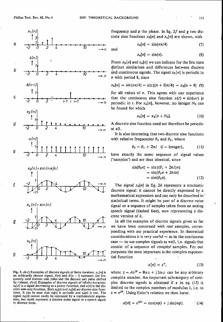
Fig. 2. a)-c) Examples of discrete signals of finite duration; Xl [n) isan arbitrarily chosen signal, ö[n) and ö[n - i) represent the fre-quently used discrete unit pulse and the discrete unit pulse shiftedby i places. d)-h) Examples of discrete signals of infinite duration;x2[n) is a signal decreasing as a power function, and u[n) is the dis-crete unit-step function. Both xs[n) and x4[n) are discrete sine func-tions. It can be seen that x3[n) is periodic and x.[n] is not. Thesignal x5[n] cannot easily be expressed by a mathematical expres-sion, but could represent a discrete noise signalor a speech signalin discrete form.
frequency and r/> the phase. In fig. 21 and g two dis-crete sine functions xa[n] and x4[n] are shown, with
x3[n] = sin(mt/4) (7)and
x4[n] = sin(n). (8)
From xa[n] and x4[n] we can indicate for the first timedistinct similarities and differences between discreteànd continuous signals. The signal xa[n] is periodic inn with period 8, since
x3[n] = sin(nn/4) = sin{(n + 8)n/4) = x3[n + 8] (9)
for all values of n. This agrees with our experiencethat the continuous sine function x(t) = sin(wt) [speriodic in t. For x4[n], however, no integer No canbe found for which
(10)
A discrete sine function need not therefore be periodicat all.It is also interesting that two discrete sine functions
with relative frequencies Ol and O2, where
O2= Ol + 2ni (i = integer), (11)
have exactly the same sequence of signal values('samples') and are thus identical, since
sin(02n) = sin {(Ol + 2ni)n)= sin(Oln + 2nin)= sin(Oln). (12)
The signal x5[n] in fig. 2h represents a stochasticdiscrete signal: it cannot be directly expressed by amathematical expression and can only be described in'statistical terms. It might be part of a discrete noisesignalor a sequence of samples taken from an analogspeech signal (dashed line), now representing a dis-crete version of it.In all the examples of discrete signals given so far
we have been concerned with real samples, corres-ponding with our practical experience. In theoreticalconsiderations it is very useful - as in the continuouscase - to use complex signals as well, i.e. signals thatconsist of a sequence of complex samples. For ourpurposes the most important is the complex exponen-tial function
(13)
where z =A ei4> = Re z + j Im z can be any arbitrarycomplex number. An important subcategory of com-plex discrete signals is obtained if z in eq. (13) islimited to the complex numbers of modulus 1, i.e. toz = ei4>. Using Euler's relation we then have:
x[n] = ei4>n = cos(nr/» + j sin(ntf». . (14)

114 A. W. M. VAN DEN ENDEN and N. A. M. VERHOECKX Philips Tech. Rev. 42, No. 4
The discrete unit pulse Oen] in eq. (2) makes it pos-sible to write any discrete signal x[n] explicitly as asequence of samples of value x[i]:
00
x[n] = I x[i] oen - i].;=-00
At this point the usefulness of this alternative mode ofexpression is not very clear; we shall return to it later.
We conclude this section with a remark on the nota-tion. Until now we have denoted discrete signals asx[n], where n represents an integer. There is thus noclear reference to absolute time (expressed in seconds,say). This may sometimes be a disadvantage, forexample if the discrete signal has been obtained bysampling a continuous signal at a sampling interval ofT seconds and we want to give a frequency descriptionin terms of absolute frequency (i.e. in Hz or rad/s).This simple notation mayalso have its disadvantagesin situations where signals with different samplingintervals Tl and T2 (in other words, with differentsampling frequencies) are to be treated simultane-ously. In all these cases [8] we shall use the equivalentnotation x[nT], x[nTI], X[nT2], etc. for x[n].
Description in the frequency domain
The Fourier transform for discrete signals (FTD)
By analogy with the theory for continuous signals a(frequency) spectrum for the discrete signal x[n T] can
x[nT)
t T,,"'--,
\,' -,\, \\ , \
" .-377: -277: -st 0 'Ir
T T T r:. 2'1r/T .1 - w
fundamentalinterval
-n
Q
x[n)
t
I 2'1r II. "I
fundamentalinterval
Fig. 3. a) Schematic representation of the spectrum X(eJwT) of asignal x[nTl, obtained with the Fourier transform for discrete sig-nals (FTD) from eq. (16). The spectrum is completely characterizedby its behaviour in the fundamental interval -nIT Sw < nIT.b) The same result when the FTD is applied in normalized form asgiven by eq. (19). The fundamental interval is now 2n. w absolutefrequency, 8 relative frequency.
be derived by means of the Fourier transform for dis-crete signals (FTD). This is defined as follows:
FTD:00
X(ejwT) = L ~[nT] e-jnwT•n=-oo
(16)(15)
A schematic example of this transform is given injig.3a. In this figure the periodicity of X(ejwT) withthe period 2n/T is at once apparent. This is one of themost typical features of the spectrum of any discretesignal. A single period is all we need to fully defineX(ejwT) and hence x[nT]. It is usual to take the inter-val -n/T $ co< nl T and to call it the fundamentalinterval. (Sometimes the interval û s; co < 2n/T maybe taken.) From the variation of X(ejwT) in the funda-mental interval we can find x[nT] by means of theinverse Fourier transform for discrete signals (IFTD):
nIT
IFTD: x[nT] = .!__ J X(ejwT) ejnwT dw. (17)21t
-nIT
The functions x[nT] and X(ejwT) constitute a pair oftransforms (or Fourier pair), which we can representsymbolically by
(18)
The analogy of the FTD and the Fourier transform for con-tinuous signals (FTC) appears most directly from a comparison ofthe relevant equations. The FTC and the corresponding lFTC aregiven by
FTC: X(jw) = J x(t) e-Jw' dl,-00
IFTC: IJ'X(I) = - X(jw) elW' dw.2n
The greatest differences are found in the replacement of the integralby a summation for the transformation from time to frequency andin the change of the integration interval for the inverse transfer-mation.The fact that we use the notation X(eJwT) for the FTD and nor,
for example, X(jw) is due to the connection between the FTD andthe z-transforrn, which we shall deal with later. It has the incidentaladvantage that the use of eiwT as a variable gives explicit expressionto the periodicity in w.
[81 Sometimes the opposite is true: little use is then made of thefact that x[nl is a function of the variable n, and one onlywishes to make a clear distinction between discrete signals andcontinuous signals. The more compact notation Xn can then beused, as in [91.
[91 M. J. J. C. Annegarn, A. H. H. J. Nillesen and J. G. Raven,Digital signal processing in television receivers. Forthcomingarticle in the special issue ofthis journalon 'Digital signal pro-cessing Il, applications'.

Philips Tech. Rev. 42, No. 4 DSP: THEORETICAL BACKGROUND 115
Besides the forms of equations (16) and (17), theFTD and IFTD also have the (more usual) normalizedforms. These are obtained by substituting n for nTand 0 for enT. We then obtain (see fig. 3b):
FTD:co
X(ej8) = L x[n]e-jn8,n=-co
IFTD:
It
x[n] = _1_ J X(ej8) ejn8 dO.21t
-It
The quantity 0 is called the relative frequency. Thereis also a fundamental interval for X(ej8), of magni-tude 21t. This interval is usually taken as -1t $ e < n.Since x[n] and X(ej8) form a Fourier pair, we canwrite:
We should realize that X(éj8) is a complex function;when making graphical representations we have to splitX(~8) into areal part R = ReX(ej8) and an imaginarypart 1= Im A'(e'") or into a modulus A = IX(ej8) Iand an argument f/J = argX(ej8), giving
X(ej8) = R + jI = A ej9\ (22)
where R, I, A and f/Jare functions ofthe frequency, sothat we really ought to write R(ej8), I(ej8), A(ej8) andf/J(ej8). The same considerations also apply of courseto X(ejwT). In fig. 3 it has been assumed for conven-ience that the spectra are purely real. A more realisticexample is given in fig. 4, where the actual FTD isshown in the two ways just mentioned for the signalx[n] = O.Sn u[n].
x In}
t 1
-2 o
6."...--------------,27rf/>(ei8 )
7r 1
-2~------------~----------~-7r
-7r 0 7r-8
The FTD has a large number of properties that correspond tothose of the Fourier transform for continuous signals. For illustra-tion we shall state here the most important properties that we shallbe using in the rest of this article. We start out from the two Fourierpairs:
(19) x[n] ~X(el9) and yIn] ~ Y(el9).
I. Linearity. For all values of the constants a and b:
ax[n] + by[n]~aX(ë) + bY(ei9).
11. Shift. For every integer i :
x[n - i] ~e-iI9 X(ei9).
Ill. Convolution. Although we shall not be dealing in detail withthe convolution operatien (indicated by *) until we get to page 122,we should mention one extremely important property here: the con-volution of two signals in the time domain corresponds to multipli-cation of their Fourier transforms in the frequency domain. Ex-pressed formally:
(20)
(21)
IV. For real signals x[n], the real part of the Fourier transform is.even and the imaginary part odd, i.e.:
or, expressed in terms of modulus and argument:
A(el9) = A(e-i9) and l/I(ei9)= .,.-1/I(e-i9).
To describe real signals, it is therefore sufficient to use the spectrumin a half fundamental interval.
The z-transform (ZT)
Besides the FTD described above there are othervery useful related signal transforms for discretesignals. An extremely important one is the (bilateral)
2 4 6 8 10--n
6 6R(ei8)
1 42 2
-2 -2
o-8
Fig. 4. Applying the FTD to a discrete signal generally results in a complex spectrum, so that twofrequency functions have to be shown. The combination usually chosen is modulus A(el9) andargument l/I(ei9) or the combination of real part R(el9) and imaginary part I(el9). Both alter-natives are shown here for the case x[n] = o.sn urn].

116 A. W. M. VAN DEN ENDEN and N. A. M. VERHOECKX
z-transforrn (ZT). The z-transforrn X(z) of a discretesignal x[n] is defined as:
ZT:co
X(z) = I x[n] z-n.n=-CIO
We see how use is made here of the complex exponen-tial function z"", where z can assume any arbitrarycomplex value. X(z) is thus a complex function of thecomplex variable z. This means that we cannot easilyproduce a direct graphical representation of all valuesof the function X(z). This would require two 3-dimen-sional figures ('hill-and-valley landscapes'), one ofwhich would for example give ReX(z) as a functionof Re zand Im z, and the other would do the same forImX(z) (fig. 5). We shall see later, however, thatthere is another very different, but effective, graphicalmethod of obtaining an understanding of the proper-ties of X(z) and x[n] (the 'poles-and-zeros plot').
The a-transform plays the same role for discrete signals as theLaplace transform (LT) for continuous signals. The (bilateral) Lap-lace transform is given by:
LT:
0:>
X(p) = J x(I) e-pt dl.
The most important difference is the replacement of the integral bya summation. The fact that the base of the naturallogarithm e canbe recognized in the LT but not in the ZT is a mere detail, since anycomplex number z can be written as:
z = 0+ jb = Aej\1) = e1n(A)+jll) = e".
With the ZT, as with the LT, the question of convergence arises.For a given function x[n) the infinite sum of eq. (23) will not 'con-verge' for every value of z to yield a finite value. For every X(z) weshould therefore, strictly speaking, mention the relevant region ofconvergence. This is particularly important from the theoreticalpoint of view, because under different convergence conditions thesame X(z) corresponds to different functions x[n). In practical sys-tems, however, there is never any doubt about which x[n) is beingdealt with. In this article we therefore do not usually consider con-vergence.
Let us now look at the ZT of the signal
xJ[n] = A ó[n - iJ.This represents a discrete pulse of amplitude A at thetime n = i. From eq. (23) we find:
co
X1(z) = L A ó[n - i] z:" = AZ-i.n=-CIC)
(25)
Similarly we find for
x2[n] = 2ó[n - 1] + 3ó[n - 2] (26)
that
(27)
On these two examples we can base an interpretation
(23)
Re X(z)
tImz,ij
Philips Tech. Rev. 42, No. 4
Im X(z)
tImz,ij
a-Rez a
++Re e
Fig. 5. Applying the z-transform to a discrete signal x[n) generallyresults in a complex function X(z) = Re X(z) + j Im X(.::) of thecomplex variable z = Re z + j Im z. In a graphical representationwe should need two 3-dimensional figures ('hill-and-valley land-scapes'). To indicate this the figure gives X(a + jb) = c + jd corres-ponding to a single value of z = a + jb.
of X(z) that can often be very useful: if X(z) has theform of a polynomial in Z-I , then the factor associatedwith the term z:' corresponds exactly to the value ofx[n] at the time n = i.
The formal counterpart of the ZT as given byeq. (23) is the inverse z-transform (IZT):
x[n] = _1_. fX(Z) Zlt-I dz.2nJ
IZT: (28)
This expression represents a contour integral in thez-plane, In practical applications it is seldom used,however, because the required inverse transform fromX(z) to x[n] can often be achieved much more simply:e.g. by using general properties of the ZT (such aslinearity) or reduction to known z-transforrns. Somefrequently occurring pairs of transforms have beencollected in Table J.
Table I. Some common pairs of bllateral z-transforms
x[n) X(z)
(24)
J[n)
ó[n - i)
u[nl
an urn)
an-1 urn - 1)
nu[n)
cos(nç) urn)
sin(nç) urn)
an sin(nç + '11) urn)
zz - 1
zZ-Q
Z-Q
z(z - 1)2
z(z + I)
(z - 1)3
Z2 -;: cosç
Z2 - 2;: cosé + 1
z sinç
Z2 - 2;: cosé + 1
z2 sin('II) + az sin{ç _ '11)
Z2 - 20;: cosç + 02

Philips Tech. Rev. 42, No. 4 DSP: THEORETICAL BACKGROUND 117
The fact that x[n] and X(z) constitute a pair oftransforms is indicated in the following way:
The most frequently used properties of the ZT relate to linearity,shift and convolution. Proceeding from the pairs of transforms
these properties are as follows:
I. Linearity. For all values of the constants a and b:
ax[nl + by[nl~ aX(z) + bY(z).
11. Shift. For every integer i:
x[n - il~ z:' X(z).
Ill. Convolution. Although the convolution operatien (indicatedby *) will not be treated until page 122, we mention the convolutionproperty in advance because it is so extremely important:
x[nl * y[nl ~ X(z) Y(z).
In the inverse transformation of a given Xo(z),which is a ratio of two polynomials in z, to the corres-ponding xo[n] it is common practice to use the tech-nique of expansion in partial fractions. This is bestexplained by an example. Suppose that
zXo(z) = ,
(z - a)(z - 13)where a and 13 are constants. In Table I we find noX(z) that immediately resembles this. We now try to 52rewrite Xo(z) with as yet unknown constants A andB, as:
Az BzXo(z) = -- +
z-a z-f3
Next we reduce everything to a common denominator:
Az(z - 13) + Bz(z - a)Xo(z) =
(z - a)(z - 13)(A + B)Z2 - (f3A + aB)z
(z - a)(z - fJ)
We now see that equations (30) and (32) are identicalwhen
A + B = 0 and f3A + aB = -1 (33)or
1A = --- and
a-f3
-1B=--.
a-fJ
We can therefore rewrite eq. (31) as:
1 (.: z)Xo(z) = -- -- - -- .a-f3 z-a z-f3
(29)
Writing the equation in this way we see two terms ofthe form z/(z - a), which occurs in Table I. Using thelinearity of the ZT we then find:
1xo[n] = -- (an - fJn) urn]. (36)
a-f3
The relation between FTD and ZT
Between the z-transform and the Fourier transformfor discrete signals a direct relationship exists: whenz = eW the ZT of eq. (23) becomes identical with theFTD of eq. (19). How can we best interpret this? Withz = ej8 and - TC :s e < TC we describe exactly all thepoints for which Iz I = 1, that is to say all the pointson the unit circle in the z-plane. This brings us toan important statement: the FTD of a discrete signalcorresponds to the ZT on the unit circle in the z-plane. This relationship can be represented graphically(jig. 6). For convenience we have chosen an X(z) thatis purely realon the unit circle, so that both for X(z)and for X(ej8
) a single diagram is sufficient.
(30)
X(z) X(eJ8)
t i8:=!. '][,
-I tt-7r/2 ][/2
b
Fig. 6. Plot of the relation between a) the ZT on the unit circle inthe z-plane (i.e. z = ej8) and b) X(ejO) obtained from the FTD. Forconvenience it is assumed that X(ejo) is purely real.
(31)
(32)
The above relationship only applies of course when the z-tr ans-form exists (in other words, when X(z) converges) on the unit circle.In most practical situations this is in fact the case. But signals thatcorrespond to the impulse response of an unstable system (see thesection 'Discrete systems') form a notorious exception. These havea z-transforrn that does not converge on the unit circle and there-fore no FTD exists.
The relations discussed so far between a discretesignal x[n], its Fourier transform X(ej8) and its z-transform X(z) are summarized in jig. 7.
(34)
The discrete Fourier transferm (DFT)
The Fourier transform for discrete signals (FTD),which we have described earlier in this article, is apowerful analytical tool for determining the frequencyspectrum of discrete signals. But it has its limitations.We shall now look at these with the aid of the FTD inthe normalized form, as given in equations (19) and
(35)

118 A. W. M. VAN DEN ENDEN and N. A. M. VERHOECKX Philips Tech. Rev. 42, No. 4
8
G IFTD
FTO 8Fig. 7. Relations between a discrete signal x[n], its Fourier trans-form X(ei8) and its z-transforrn X(z). ZT z-transform. lZT inversez-transform. FTD Fourier transform for discrete signals. lFTOinverse Fourier transform for discrete signals. The transition fromX(z) to X(ei8) and vice versa is a simple substit ution: z = ei8. (It isassumed that the relevant transforms do really exist.)
x fn}=cos(27rnI6)
~c,; -n
precisely, the N-point discrete Fourier transform (N-point DFT). This is defined as follows:
N-l
N-point DFT: XN[k] = I XN[n] e-j(2njN)kn. (37)n=O
The cortesponding inverse transform is:
1 N-l .N-point IDFT: xN[n] = - I XN[k] eJ{2n/N)kn. (38)
N k=O
Using the OFT we can thus calculate N values of thediscrete frequency function XN[k] from the signalxN[n]. From this, using the corresponding 10FT, wecan then retrieve the original N values of xN[n] exactly.The two functions xN[n] and XN[k] thus constitute aregular pair of transforms, which is represented sym-bolically by:
(39)
£_0;, 31XNft
N=6 Li______l_00 1 2 3 4 5
--k
--n
OFTo----<:l
N= 12 6
00 2 4 6 8 11--k
OFT0----<)
N=16 {L~00 2 4 6 8 10 15
--k
c
--n
Fig. 8. Example of the application of an N-point OFT for different values of N to the periodic sig-nal x[nl = cos(27tnf6). It is advisable to choose N equal to an integral number of periods of x[n],for example N = 6 (case a) or N = 12 (case b). Otherwise there is 'leakage' of the spectral cornpo-nents (case c). For N = 6 and N = 12 a purely real spectrum is found. For N = 16 the spectrum iscomplex and only the modulus IXN[kJ I is shown.
(20). In the first place we may note that eq. (19) is notdirectly applicable to periodic signals x[n]; the sum-mation of an infinite number of terms will then presentdifficulties. Nor is such an infinite summation verymeaningful if x[n] is of finite duration and thereforediffers from zero only for a finite number of valuesof n. In addition, computer calculation of the IFTOfrom eq. (20) requires a numerical calculation (hence:approximating) of the relevant integral. It has there-fore been helpful to introduce another aid, in the formof the discrete Fourier transform (OFT), or, more
To illustrate the application of the OFT we shallfirst take a simple periodic function. Let us choosex[n] = cos(2rcn/6), with three different values of N: 6,12 and 16 (fig. 8). The function x[n] is periodic withthe period No = 6, since x[n] = x[n + 6] for all n.
We now see in fig. 8 that it is important when apply-ing the OFT to periodic signals of period No to takethe length N equal to No or an integral multiple of No(cases a and b). If this is not so (case c), the discretespectrum XN[k] does not contain the 'right' frequencypositions for representing the original periodic signal

Philips Tech. Rev. 42, No. 4 DSP: THEORETICAL BACKGROUND 119
x[n]. We then find contributions at all values of k, aneffect known as 'leakage'.From a comparison of cases a and b we also see that
a larger N gives greater spectral resolution. The spec-trum XN[k] shows a high degree of symmetry becausexN[n] is a real function; in Fourier transformation thisalways results in such properties (see for examplewhat was said in small print on page 115 on the pro-perties of the FTD).At the beginning of this subsection we suggested
that the N-point DFT can be used to calculate thespectrum XN[k] of a discrete signalof finite duration( $.N). This leads us to ask whether there is a relationbetween XN[k] and the spectrum X(ej8
) that can becalculated for the same signal with the FTD in eq. (19).This is in fact the case. A direct comparison of equa-tions (37) and (19) shows that the following simplerelation exists between these two spectra:
Expressed in words: for a discrete signalof finiteduration NI, the N-point DFT is a sampled version ofthe FTD, provided that NI $. N. To illustrate thisrelationfig. 9 shows the FTD and the 8-point DFT fora discrete signal x[n] of finite duration NI = 4.
We have assumed above that we are considering both xN[nj andXN[kj for nand k between 0 and N - I. However, the complexexponential functions e-j(2n/N)kn and eJ(2n/N)kn are periodic in kand jn n with period N. If we calculate XN[kj in eq. (37) for k < 0or k > N - I, we therefore find the same values as we found foro $ k $N - I. Similar considerations apply to xN[nj in eq. (38).We can therefore say that xN[nj and XN[kj are periodic functions ofperiod N, and only the fundamental interval between 0 and N - 1 isof significanee in the transformation process.
The fast Fourier transform (FFT)
In addition to the transforms described so far, theterm FFT (for 'fast Fourier transform') is often en-countered in the literature on discrete signal pro-cessing. This is not another type of transformation,however, but refers simply to a very effective mannerof calculating the DFT. The name FFT is really a col-lective name for various interrelated calculationmethods and stratagems.If we again look at equations (37) and (38) for the
DFT and the IDFT, we see that for each result (each'point') of the transformation we have to perform Ncomplex multiplications and N - 1 complex addi-tions. For a complete N-point transformation thisamounts to N2 and N(N - 1) respectively. A directcalculation of an N-point DFT thus requires a numberof complex operations of the order of magnitude ofN2
• For N = 4 this is 16, but for N = 2048 we arealready at N2
~ 4194304. In the practical application
(40)
RrJ1DHo 7r21f
3lu_) -10 --. eFTD-IFTD IrJ1D~-
-2 0 2--.n o 27r 7r
-10 . - e
RNlk}
t 10 ,,,0
'N{"tL-10
OFT10FT [NIk}-N=8 t 10
02 4 6--. n 0
Fig. 9. Comparison of the FTD and the 8-point DFT of a discretesignal x[nj of finite duration NI = 4. It is clear that the DFT spec-trum XN[kj = RN[kj + jIN[kj is a sampled version of the FTDspectrum X(eJB) = R(eiB) + jI(eiB).
of the DFT this number of operations is of consider-able importance, since it determines the time and thetype of equipment we need. For nearly 200 years, andespecially in the last twenty or thirty years [10], therehas therefore been keen interest in methods that makeit possible to calculate an N-point DFT with feweroperations. The procedure always followed is first tocalculate a number of DFTs of smaller length andthen to combine the results in an appropriate way. IfN is even, an Nl2-point DFT can be performed firston all the even-numbered samples of xN[n] and thenon all the odd-numbered samples. Next, the requiredN-point DFT can be calculated from the results ofthese two smaller DFTs. Altogether this requiresfewer calculations than a direct procedure. If NI2itself is also an even number, this procedure can berepeated. The most familiar are therefore the FFTalgorithms, in which N is an integral power of two,so that N = 2M• The same procedure can then berepeated as many as M times. In this way the totalnumber of operations is of the order of Nx M, whichis a reduction by a factor of NIM. The very substan-tial effect of the FFT compared with a direct calcula-tion of the DFT, especially for large N, is evidentfrom fig. la.
(10) M. T. Heideman, D. H. Johnson and C. S. Burrus, Gauss andthe history of the fast Fourier transform, IEEE ASSP Mag. I,No. 4 (October), 14-21, 1984.

120A. W. M. VAN DEN ENDEN and N. A. M. VERHOECKX Philips Tech. Rev. 42, No. 4
10x105r------- ~
Nopi 86
N NIM2 2.0I. 2.08 2.716 1..032 6.1.61. 10.7128 18.3256 32.0512 56.91021. 102.1.201.8 186.2
4
2
00 128256 512 1024-N
Fig. 10. Comparison of the number of operations Nop required fora direct calculation of the N-point DFT and for a calculation madewith the FFT. Only values of N that are an integral power of 2 areconsidered: N = 2M• The number of operations is then reduced bya factor of NIM. This is indicated for a number of values of N in aseparate table.
11. DISCRETE SYSTEMS
Now that we have dealt with a number of funda-mental theoretical aspects of discrete signals, we canturn our attention to discrete systems. Quite generally,a discrete system is defined as a system that convertsone or more discrete input signals x[n] into one ormore discrete output signals yen] in accordance withcertain discrete rules. In the following we shall be con-cerned mainly with systems with one real input signalx[n] and one realoutput signal yen]. For the timebeing we shall also confine our considerations to thevery important category of linear time-invariant dis-crete systems (LTD systems). For practical purposesthese include most discrete (and hence digital) filters.
A discrete system is linear when the input signal aXl[n] + bX2[n]produces an output signal ayJ[n] + bY2[n], where a and barearbitrary constants. Here, xJ[n] and x2[n] are arbitrary input sig-nals and yJ[n] and Y2[n] are the corresponding output signals.A discrete system is time-invariant if the input signal x[n - i]
produces an output signal YIn - i], where i is an arbitrary integer,x[n] an arbitrary input signal and YIn] the corresponding outputsignal.
For practical purposes, discrete systems should also possess thefollowing two properties: stability and causality.A discrete system is stable if any arbitrary input signalof finite
amplitude (i.e. Ix[n] Imu $ A) produces an output signalof finiteamplitude (i.e. Iy[n] Imax sB).
A discrete system is causal if at any instant n = no the outputsignal corresponding to any arbitrary input signal is independent ofthe values of the input signal later than no. (Loosely formulated:there can be no output signal before there has been an input signal.)In the rest of this article the term 'practical' implies the concept'causal'.
LTD systems have a number of particularly attrac-tive properties. The first is that all feasible systems ofthis type can be composed of only three basic elements(fig.lJ):
x-In]
~ yln}=xdn}+x2In}~o
x2ln}
x()o/_n_}__-I~[9>--__ !oIn} = Ax In}
x In} J,:'l _yln}=xln-1}o------.~o
,Fig. 11. The three basic elements from which all realizable lineartime-invariant discrete systems (LTD systems) can be built up.a) Adder. b) Multiplier by a constant factor A. c) Unit-delay ele-ment. T unit delay or sampling interval.
xln} yIn}
vIn}
Fig. 12. a) The combination of an adder with a multiplier by a fac-tor of -1 results in a subtracter. b) Example of a simple LTD sys-tem containing all the basic elements. In addition to the input andoutput signals a number of internal signals ('intermediate results')are indicated.
• the adder, in which two input signals are added toform one output signal,• the multiplier, in which a signal is multiplied by aconstant, and• the unit-delay element, in which the input signal isdelayed by one discrete time unit (sampling interval).
By combining these elements we can make otherfunctions, for example a subtraeter (fig. 120). An-other simple but realistic LTD system is shown infig. l2b. Later we shall analyse the filter properties ofthis circuit.A close relation exists between the theory of dis-
crete signals, which we have dealt with in the fore-going, and the theory of LTD systems. There is a goodexplanation for this, since the most important proper-ties of an LTD system can be derived from only onediscrete signal - the output signal that is obtainedwhen the input signal is the discrete unit pulse oen].We call this output signal the impulse response hen] ofthe LTD system (fig. 13).

Philips Tech. Rev. 42, No. 4 DSP: THEORETICAL BACKGROUND 121
where ai and bi are real constants. Equation (44) is its impulse response is given by:called a linear difference equation (of the Mth order)with constant coefficients. hc[n] = ~oen] - 2( - ~)n urn].
y~
Q -n -n
xfnJ=MnJ
Lylol=blnl
~-n -n
Fig. 13. 0) Like any other discrete system an LTD system convertsan input signal x[n) into an output signal yIn). b) The special.feature of an LTD system is that it can be characterized by its im-pulse response h[n); this is the output signal yIn) = h[nl corres-ponding to the input signal x[n) = ó[n).
Signal transforms such as the FTD or the ZT can beapplied to the impulse response hen]. We then obtainalternative descriptions of the LTD system for whichwe use separate names. Applying the FTD to hen] weobtain the frequency response H(ej8). Applying theZTto hen] we get the system function H(z). We knowfrom the foregoing that:
The frequency response and the system functionconstitute descriptions of the system in the frequencydomain. The impulse response, on the other hand,gives a description of the system in the time domain,as do also the difference equations. We shall considerall these four modes of description in somewhat moredetail, starting with the last.
System descriptions
Difference equations
Let us look again at the system of fig. 12b. We candescribe this system by the following simple equations:
ven] = ax[n] + bx[n - 1] + yen - 1]y[n] = even].
(42a)(42b)
Eliminating v[n]:
y[n] = acx[n] + bcx[n - 1] + cy[n - 1]. (43)
This equation will give us the present value of the out-put signal if we know the present input signal and theprevious values of the input and output signal. Quitegenerally, a practical LTD system can be described by:
N Myen] = L bix[n - i] + L aiy[n - i], (44)
i=O i=l
Equation (44) is the discrete counterpart of the linear differentialequation with constant coefficients that can be used to describepracticallinear time-invariant continuous systems, which is writtenas follows:
N M
I dkx(t) I dky(t)y(t) = bk-- + Ok--.
dtk dtkk=O bi
The description of a discrete system by a differenceequation is important for two main reasons. In thefirst place it is a good starting point for deriving othersystem descriptions, such as the system function. Inthis case the difference equations are replaced byalgebraic equations. Calculation with these is muchsimpler, as we shall see. In the second place a differ-ence equation gives a direct indication of a possiblestructure for a system. For instance, a system that isdescribed by the difference equation
3 3yen] = L bix[n - i] + L aiy[n - i], (45)
i=O i=l
can be realized with the circuit shown infig.14. It willappear later that there are many other structures withthe same difference equation.
(41)
Fig. 14. LTD system described by the difference equation given ineq. (45)..
Impulse response
Sometimes the impulse response of a discrete sys-tem can be derived directly from the block diagram;sometimes it is more complicated. This will becomeclear from a few examples. For fig. 15a it is fairly easyto see that:
hA[n] = 2o[n] - ~ó[n - 1],
and for fig. 15b
hB[n] = (- ~t+lurn].
(46)
(47)
Although fig. 15c is only the cascade arrangement of(a) and (b), it is perhaps less obvious at this point that
(48)

122 A. W. M. VAN DEN ENDEN and N. A. M. VERHOECKX Philips Tech. Rev. 42, No. 4
6~n]1 xlnl
.l_ 2
ylril_nQ -1
hBhn]t 1
-1 -n
-2Fig. IS. Simple LTD systems with corresponding impulse response.The system in c) corresponds to the cascade arrangement of (a)and (b).
In principle it is not difficult to see that we can usethe impulse response of an LTD system to calculatethe output signal for any arbitrary input signal. To dothis we return to eq. (15), which we now recapitulate:
00
x[n] = I x[i] ó[n - i]. (49);=-00
In this equation x[n] is expressed as a series ofweighted unit pulses, where the ith pulse has theweight x[i]. Since we are dealing with a linear time-invariant system, this ith pulse produces an outputsignal x[i]h[n - i]. Therefore
x[i]ó[n - i] ~ x[i]h[n - i]
and
;=-00 ;=-00
co 00
I x[i]ó[n - i]~ I x[i]h[n - i]. (51)
In this way, then, we have found the exact output sig-nal yen] corresponding to x[n] as given by eq. (49):
00
yen] = I x[i]h[n - i];=-00
or00
yen] = I x[n - i]h[i].;=-ct:>
by i.) Equations (52a) and (52b) represent the con-volution of x[n] and hen]. We can abbreviate this to:
yen] = x[n] * hen] = hen] * x[n]. (52c)
- n Summarizing: the output signalof an LTD system canbe obtained from the convolution of the input signaland the impulse response.
It is very easy to see whether an LTD system is stable or causal(or both) from its impulse response h[n]. For a stable LTD systemwe have:
00
L Ih[nll =C<co.nz-co
For a causal LTD system we have: h[n] ~ 0 for n < O.
Frequency response
Instead of the impulse response hen] we often con-sider the corresponding FTD, i.e. the frequency re-sponse H(ej8). One of the main reasons for doing thisis the convolution property of the FTD: the convolu-tion of two discrete signals x[n] and hen] correspondsto the multiplication of their FTDs. This provides uswith a second means of calculating the output signalyen] from an input signal x[n].• We first determine X(ej8) and H(ej8).• We multiply X(ej8) by H(ej8); this gives the FTDof yen]:
(53)
(50)
• We apply the IFTD to Y(ej8) and thus find yen].
Both methods of calculating yen] are shown schema-tically in fig. 16. The method using the FTD is oftenpreferable because it requires the least calculation.The second important virtue of the frequency re-
sponse as a system description is the intuitive ease withwhich it is often possible to analyse discrete systems,especially filters, from their amplitude and phasecharacteristics, which are merely the modulus andargument ofthe FTD. A simple LTD system is shownas an example in fig. 17. The impulse response hen] isgiven by: .
hen] = an urn]. (54)
For the frequency response H(ej8) we then find from(52a) eq. (19):
00 00 coH(ej8) = I h[n]e-jn8 = I ane-jn8 = I (ae-j8)n.
n=-oo n=O n=O (55a)(52b) If lal < 1, we can then write:
(Equation (52b) is obtained from (52a) by substitutingj = n - i in the right-hand side and then replacing j
, 1(55b)
1 - acosB + aj sinB

Philips Tech. Rev. 42, No. 4
BB\/c:J
Q
DSP: THEORETICAL BACKGROUND 123
I X(ei9) I I H(ej9) I"10./
D~
I Y(ej9) IIIFTD
~
Fig. 16. With a given input signal x[n) and impulse response h [nI ofan LTD system there are two different methods of calculating theoutput signal y[n). a) Direct calculation using the convolutionoperation. b) Calculation by a succession of two FTDs, multiplica-tion and IFTD.
25dB
20
-10
Fig. 17. Simple LTD system with impulse response h[n) = an u[n)and corresponding amplitude characteristic A(eJ9), on a dB scale,and phase characteristic Q)(eJ9) for different values of a.
Y Y/?!
"yln-1[~· Yln-tJ0=]Q
Fig. 18. Direct determination of H(z) = Y(z)/X(z) from the blockdiagram of an LTD system. a) Original block diagram in the timedomain. b) Corresponding block diagram in the z-dornain.
If we also use eq. (22) we find for the amplitude andphase characteristic:
A(ej8) = (56)VI + a2 - 2a cos8
and
. ( -asin8 )(/J(eJ8) = arctan .1 - a cos8
(57)
These characteristics are shown in fig. 17 for variousvalues 0 < a < 1.
System function
The most abstract but at the same time the mostversatile description of an LTD system is given by thesystem function H(z), which we can obtain as thez-transform of the impulse response h [n]. In the firstplace we can use the convolution property of the ZT,which states that convolution of two discrete signals(see eq. 52) corresponds to multiplication of the as-sociated z-transforms. If x[n] is the input signal andy[n] the output signalof an LTD system with impulseresponse h[n], then:
Y(z) = X(z)H(z). (58)
We can rearrange this as:
H(z) = Y(z)/X(z). (59)
Here we have a second, often very effective, mannerof determining H(z), since the ratio on the right-handside of eq. (59) can easily be derived from the differenceequation of an LTD system. As an example let us takethe difference equation of eq. (43). If we apply the ZTterm by term (this is permissible because of the linear-ity of the ZT), we find
Y(z) = ac X(z) + bcz:" X(z) + cz-1 Y(z). (60)
This gives:
Y(z) • ac + bcz-1H(z) = X(z) = 1 _ cz-1
In the same way we find from the general differenceequation of a practical LTD system (eq. 44):
(61)
N
L b.z:'H(z) = _Y_(z_)= _;_i=O,,-=- __
X(z) M1 - L aiz:'
i=1
(62)
In practice the analysis of an LTD system is oftenbased on a block diagram. To determine the systemfunction the difference equation is usually omitted asa separate intermediate step and a direct description ismade by means of z-transforrns. Considerable use is

124 A. W. M. VAN DEN ENDEN and N. A. M. VERHOECKX Philips Tech. Rev. 42, No. 4
made here of the property that a delay of one samplinginterval in the time domain corresponds to multiplica-tion by Z-I in the z-domain. This procedure is illus-trated in jig. 18 for the system of fig. 17. It is easilyseen from fig. ISb that:
Y(z) = X(z) + az-I Y(z),
so that
Y(z)H(z) = -_ = -----:-
X(z) - az-I'
By substituting z = ejO we also find the frequency re-sponse determined earlier, though more laboriously,in eq. (55).
Poles and zeros
In eq. (62) we have already found that the systemfunction H(z) of practical LTD systems takes theform of a ratio of two polynomials in Z-I, i.e.:
bo + blz-I + b2z-2 + ... + bNz-NH(z) = -1 -2 -M' (65)
1 - alz - a2z - ... - aMz
We can always rewrite the numerator and denomina-tor as a product of factors:
(z - ZI)(Z - Z2) ... (z - ZN) M-N (66)H(z) = bo z .(z - PI)(Z - P2) ... (z - PM)
The precise (complex) values ZI. Z2, ... , ZN andPI. P2, , PM depend on the (real) coefficients bo,bi, bz, , bs, al, 02, ••• , OM in eq. (65). For z =ZI. Z2, ••• , ZN the value of H(z) is zero and for z =PI.P2, .. "PM the value of H(z) is infinite. We there-fore speak ofthe zeros Zj (i = 1, ... ,N) and the polesPi (i = 1, ... ,M) of the system function H(z). If someZj(or Pj) are equal to each other, we speak of multiplezeros (or multiple poles). The factor ZM-N in eq. (66)corresponds formally to an (M - N)-fold zero (ifM> N) or to an (N - M)-fold pole (if N> M) atZ = O. On the other hand, we know that this factoronly represents a simple shift of h[n] in time andtherefore generally neglect it. We see that the polesand zeros fully determine the function H(z) and hencethe corresponding LTD system, except for a constantfactor boo The positions of poles and zeros are easilyvisualized in the complex z-plane. This gives thepoles-and-zeros plot of H(z), which is a very usefulgraphic aid. Fig. 19 gives an example for an arbitraryLTD system. We shall now use this figure and thefollowing, to make some remarks of general validityfor practically feasible systems, but we shall offer noderivations or proofs.• With real coefficients bo, ••. , bN, al, ... , OM, polesand zeros can only be real or occur in complex con-jugate pairs (the poles-and-zeros plot is therefore al-
(63)
ways symmetrical with respect to the horizontal axis).• Since the frequency response corresponds to the sys-tem function on the unit circle in the z-plane, each poleand each zero has the most effect on the frequencyrange associated with the nearest part of the unitcircle. Furthermore, the effect of a pole or zero on thefrequency response increases the closer it is to the unitcircle. In the extreme case of a zero actuallyon theunit circle, e.g. at z = ej81, the amplitude of the fre-quency response is zero at 8 = 81 and there is a jumpof 1t radians in phase at that point. On the other hand,a pole on the unit circle, e.g. at z = ej82, gives an in-finite amplitude at 8 = 82, again with a phase jump of1t radians.• In a stable system all the poles are inside the unitcircle; zeros may lie inside it, on it, or outside it.• If all the zeros are inside the unit circle, we have a'minimum-phase network' (jig. 200), if they do not wehave a 'non-minimum-phase network' (fig. 20b). Thesystems in fig. 200 and b have the same amplitudecharacteristics, because the zeros of one case are theexact 'reflections' of the zeros of the other case in theunit circle (i.e. the zero Zj= rjej8j is replaced by thezero z, = (l/rj)ejOI).
• If all the poles are inside the unit circle and all thezeros are outside it, and if poles and zeros are alwaysreflections of one another in the unit circle, we have aconstant-amplitude system (a phase-shifter or allpassnetwork); see fig. 20c.• If a system (except for the origin) has poles only, wecall it an 'all-pole' system (fig. 20d).• If a system (except for the origin) has zeros only,and these are reflected in pairs in the unit circle (pos-sibly also with zeros on the unit circle) then the phasecharacteristic is strictly linear and we have a Iinear-phase system (fig. 20e).
(64)
Imz
t 1
xo
-Rezo x
Fig. 19. Poles-and-zeros plot for an arbitrary LTD system. x pole.o zero. The poles are realor form complex conjugate pairs. Thesame applies to the zeros. The diagram is therefore symmetricalwith respect to the horizontal axis. (In a realizable stable system allthe poles must lie inside the unit circle.)

Philips Tech. Rev. 42, No. 4
Imzt 1
g
+Re z
Imzt 1
-'Ir o -8
-'Ir o -8A(ejBj
t 1.5--1+---
0.5
-'Ir o 'Ir-8
-'Ir o -8
g . o -8
DSP: THEORETICAL BACKGROUND 125
-'Ir
-'Ir
-'Ir
-'Ir
-'Ir
Fig. 20. Poles-and-zeros plots of some realizable types of LTDsystems with corresponding amplitude and phase characteristics.a) Minimum-phase system. b) Non-minimum-phase system. c) All-pass system or phase shifter. d) All-pole system. e) Linear-phasesystem.
Ill. DISCRETE FILTERS
By far the most important representatives of theLTD systems are the LTD filters, which we shall justcall discrete filters from now on. We define a filterhere as a circuit (or an algorithm) that converts aninput signal into an output signal whose spectrum isrelated to the spectrum of the input signal in a speci-
fundamentalinterval
Fig. 21. Examples of the amplitude characteristic of ideal discretefilters: a) lowpass, b) highpass, c) bandpass, d) bandstop. (Toemphasize the periodic nature of the frequency response the fre-quency interval shown here is larger than the fundamental interval-7t:;;8<1t.)
fied way (e.g. certain frequency components may beattenuated or completely suppressed).The different ways in which a filter can be character-
ized lead to different kinds of categorization. As withthe continuous filters, we can classify discrete filtersby the type of frequency response (i.e. by amplitudeand phase characteristics). The filters whose ampli-tude characteristic is the main feature can be sub-divided into• lowpass filters,• high pass filters,• bandpass filters and• bandstop filters.Examples of idealized filters are given in fig. 21.
Just as in the case of continuous filters, transforma-tion rules that convert a filter of one type into a filterof one of the other types also exist in the discrete case.
In addition to the types of filter mentioned above,there are filters whose phase characteristic and ampli-tude characteristic both have to meet exact specifica-tions. Two examples have already been encountered:the phase-shifter (allpass network) with a constantamplitude characteristic and a precisely defined phasecharacteristic. This filter can be used in combinationwith any type of filter in fig. 21 to obtain not only aspecified amplitude characteristic but a required phase

126 A. W. M. VAN DEN ENDEN and N. A. M. VERHOECKX Philips Tech. Rev. 42, No. 4
characteristic as well. The other example relates to fil-ters with accurately linear phase characteristics. Thesefilters are useful in applications such as TV and datatransmission. The impulse responses of linear-phasefilters have considerable symmetry, as we shall see.
Other examples of special filters are:• the differentiator
Ho(è') = jO, -1t :5 0 < rr:• the integrator
H1(ej8) = I/jO, -1t:5 0 < 1t;
• the HiIbert transformer
HH(ej8) = {-~' -1t:5 0 < 0+J,0:50<1t.
It can also be very useful to classify discrete filtersby the duration of the impulse response:• if it is finite, the filter is known as a Finite ImpulseResponse (FIR) filter;• if it is infinite, the filter is called an Infinite ImpulseResponse (UR) filter.These two types differ in many respects, and some ofthe principal differences are mentioned below.• System function: away from the origin, an FIR fil-ter can only possess zeros, an HR filter can have bothzeros and poles.• Phase characteristic: an FIR filter can have anexactly linear. phase; an HR filter can be a phaseshifter.• Stability: an FIR filter is always stable, an HR filteris unstable if for some reason or other one or morepoles lie on the unit circle or outside it.A few other differences will be encountered later underthe headings 'Discrete filter structures' and 'Methodsof designing discrete filters'.
Discrete filter structures
Besides the. more fundamental classificationstouched on in the previous section, we can also classifydiscrete filtersby structure, as indicated by their blockdiagram. This alone is sometimes sufficient to permitcertain general conclusions to be drawn about thecharacteristics of a particular filter. In addition, wehave to remember that a particular structure is rarelyunique: a particular specified filter characteristic canusually be achieved with different structures - oftenvery many.
Significant differences in characteristics between structures mayalso be found when the finite-word-length effects of digital filtersare taken into account. We shall return to this point later on (pages128 and 141).
The first aspect of filter structures to be consideredis the combination of simple filters or 'filter sections'to form complex filters. This is done mainly by con-necting the filters in cascade or in parallel (fig. 22). In
g Hc(z)
Hp(z)
Fig. 22. Composite filters can be obtained by a) cascading: Hc(z) =HJ(z)H2(Z), and b) parallel connection: Hp(z) = Ha(z) + H.(z).
/~////
t{-/
B< >0Fig. 23. Usually an FIR filter has an NRDF structure and an RDFstructure gives an HR filter. In rare cases the combination of theRDF structure and an FIR filter is found (if all the poles coincidewith zeros).
g
Fig. 24. a) Arbitrary example of a discrete filter with a non-recur-sive structure (NRDF). b) A transversal filter is an NRDF in whichonly the input signal is stored in the delay elements. In this case thesuccessive samples of the impulse response have the exact values ofthe successive coefficients.

Philips Tech. Rev. 42, No. 4 DSP: THEORETICAL BACKGROUND 127
a cascade arrangement we obtain the overall systemfunction by multiplying the individual system func-tions:
The zeros of Hc(z) are therefore the zeros of HI(z)plus the zeros of H2(z), and the poles of Hc(z) are thepoles of HI(z) plus the poles of H2(z). If a zero ofHI(z) coincides with a pole of H2(Z) (or vice versa),they compensate each other and cannot then be foundseparately in Hc(z). In a parallel arrangement the in-dividual system functions have to be added together:
Hp(z) = Ha(z) + H4(z).
The poles of Hp(z) here again consist of the sum ofthe poles of the subsystems, but it is not easy to makeany general comment about the relation between thezeros.From their structure, discrete filters can be simply
classified as:• recursive discrete filters (RDFs), in which there is atleast one feedback path (e.g. fig. 15b, e), and• non-recursive discrete filters (NRDFs), in whichthere is no feedback at all (e.g. fig. 15a).
It is often wrongly assumed that an RDF structure always givesan UR filter and that an FIR filter always has an NRDF structure.Although this is usually the case, it is not necessarily so. The oppo-site is however true. An UR filter requires an RDF structure and anNRDF structure always yields an FIR filter (fig. 23).A discrete filter is said to be canonical when it contains the mini-
mum number of delay elements theoretically necessary to give thesystem function.The feedback paths that characterize RDFs introduce closed
loops. Each closed loop must contain at least one delay element,otherwise the resultant system will not be realizable because of theparadoxical requirement that the value of a signal sample must beknown before it can be calculated.
NRDFs
A filter with a non-recursive structure is shown infig. 24a. The system function H(z) and the impulseresponse h [n] of this filter are:
H(z) = (a + bz-I)(1 + ez-I) = a + (b + ae)z-l + bcz-2
(69a)h[n] = aö[n] + (b+ac)ö[n - 1] + bcö[n - 2]. (69b)
I •
It is easily seen that the impulse response of an NRDFcan never be longer than the number of unit-delay ele-ments that the filter contains, plus one. A commontype of NRDF is the transversal discrete filter (fig.24b).[11] J. J. van der Kam, A digital 'decimating' filter for analog-to-
digital-conversion in hi-fi audio signals. Forthcoming article inthe special issue of this journalon 'Digital signal processing U,applications' .
(67)
It is characterized by the fact that the only signal thatis stored in the delay elements is the original inputsignal x[n]. The system function H(z) and the impulseresponse h[n] of this filter are
H(z) = bo + blz-l + ... + bNz-N (70a)h[n] = b« ö[n] + bi ö[n - 1] + ... + bNö[n :....N].
(70b)
(68)
In this case we immediately recognize the impulse re-sponse in the filter coefficients. With a transversal fil-ter we can therefore see almost at a glance whether wehave a linear phase characteristic, the requirementbeing a symmetric or antisymmetrie impulse responseof arbitrary length N, i.e. h [i] = h [N - i] or h [i] =-h[N - i] for i = 0, ... ,N.Although only FIR filters can be made with an
NRDF, which means for instance that the relevant sys-tem function can contain 'no poles (except for the ori-gin), a good approximation to almost any frequencyresponse can be obtained by making the length Nsufficiently large. In practice we can have NRDFs withan impulse response comprising hundreds or thou-sands of samples [11]. (The system function in such acase also contains hundreds or thousands of zeros.)
RDFs
One possible structure for recursive discrete filtersfollows directly from the general description of dis-crete filters in eq. (44). This is shown infig.25a and issimply named'. the 'direct-form-I structure'. We can
x/ni
9
Fig. 25. Two examples of general structures for recursive discretefilters (RDFs). a) Direct-Ierm-I structure. This comprises M + Nunit-delay elements. b) Direct-forrn-Il structure. In the examplegiven here (M> N) this only requires M unit-delay elements.

128 A. W. M. VAN DEN ENDE~ and N. A. M. VERHOECKX Philips Tech. Rev. 42, No. 4
think of it as split up into a transversal part with filtercoefficients bo, blo ... , b» followed by a purely recur-sive part with filter coefficients al, 02, ••• , OM. Thisstructure requires a total of M + N unit-delay ele-ments. If the recursive part and the transversal partare made to change places (this is permissible becauseeach part is an LTD system in itself), the result is the'direct-form-II structure' (fig. 25b). This only containsM unit-delay elements ifM> N (or N ifN >M). Thesystem function is the same in both cases; the zerosare determined by the coefficients bi and the poles by
1st-order section 2nd-order section
Fig. 26. Third-order filter produced by cascading a Ist-order sectionand a 2nd-order section. Filters of arbitrarily high order can bemade by cascading such sections, without the high sensitivity tocoefficient variation which characterizes the direct-form structures.
the coefficients ai. A disadvantage here is that eachcoefficient bi affects all of the zeros. The same thingapplies for each ai and all of the poles. This meansthat even small changes in the coefficients can have aconsiderable effect on the frequency response of thefilter. This is a less desirable feature: it is a seriousdrawback if for example we have to use quantized (i.e.slightly modified) coefficient values in a digital filter.A solution to this problem can be found by buildingup the total filter from smaller units (see fig. 22) inwhich each pole and each zero is determined by asmaller number of coefficients. A very advantageousand widely used arrangement is a cascade of 1st-orderand 2nd-order filter sections. With a 1st-order sectionone pole and one zero that are both real can be deter-mined. With a 2nd-order section two poles and twozeros can be determined, which can be either realorcomplex (fig. 26).
Special filter structures
Comb filters
An interesting type of filter, known as a comb filter,is obtained from any given discrete filter with the sys-
Q
Hr'l \/-7r 0 7r
-(}
-..n-7r 0 n:
-(}
Fig. 27. Schematic representation of the frequency responsesH(eJ8),G](eJ8) and G2(eJ8). a) Original filter. b) Comb filter obtained from(a) with N = 3; c) as (b) but with N = 4.
tem function H(z) by replacing each unit-delay ele-ment by a cascade arrangement of N unit-delay ele-ments. This results in a new filter with the systemfunction G(z):
(71)
This means that the frequency response in the funda-mental interval (-1t :5 () < n) is periodically repeatedN times, as illustrated schematically in fig. 27 forN = 3 and N = 4. An interesting type of comb filter,which is also one of the oldest, is shown in fig. 28. Insome applications N can be 100, 1000 or even more [91.
Ladder and lattice filters
In recent years there has been a marked growth ofinterest in the filter structures known as ladder filtersand lattice filters. Some typical examples are given infigs29 and 30. There are, however, a large number ofvariations. The common feature of these filters is thatthey are built up from basic units (see the shaded partsof the figures), each with two inputs and two outputs.Lattice filters, as the name suggests, are typified by acrossover structure within the basic unit. These filtersare interesting mainly because of the following fea-tures:• the stability of the filter can be expressed in terms ofspecifications for each coefficient separately, and• the frequency response is not very sensitive to varia-tions in the precise value of the coefficients.These filters are often used for processing of discretespeech signals [121.
(12) L. R. Rabiner and R. W. Schafer, Digital processing of speechsignals, Prentice-Hall, Engiewood Cliffs, NJ, 1978.

Philips Tech. Rev. 42, No. 4 DSP: THEORETICAL BACKGROUND 129
I} 1 2 3 N-1 NL-m-S-yIn}
o• +Q
2
\1
2][/20
-][ o---8
-s-Re z
Fig. 28. a) Block diagram of one of the oldest types of comb filter,which is particularly useful for colout-Tv applications. b) Corres- Qponding poles-and-zeros plot for N = 20. c) Corresponding ampli-tude and phase characteristic for N = 20.
Q
+
Fig. 29. a) Ladder filter with a system function H(z) that only con-tains poles. b) Ladder filter with poles deter mined by the a's, andzeros determined by the /]'s. (The shaded area indicates a basic unitwhich is regularly repeated.)
yIn}
Q
it
+
x Inl yIn}
"1).,
+-1\ + t-------~'... ~'"
Fig. 30. a) Lattice filter with a system function that only containspoles. b) Lattice filter with poles determined by the a's, and zerosdetermined by the [J's. c) Lattice filter containing only zeros in thesystem function.
Q
o-[j>- + )+- _. ~I
8!>- +
o.---~ + )+- ~------~I +
Fig. 31. a) Wave digital filters are obtained by 'translating' the corn-ponents of analog filters into discrete components on the basis ofwave equations. This is indicated here for a capacitance and aninductance. b) The discrete components thus obtained are con-nected by adaptors, which only contain adders and multipliers. Theexample shown here is one of many possible types of adaptor.

130 A. W. M. VAN DEN ENDEN and N. A. M. VERHOECKX Philips Tech. Rev. 42, No. 4
Wave digital filters
Wave digital filters, or WDFs, are a category apart.They can be obtained from a direct 'translation' of agiven analog filter on the basis of wave equations. Acapacitance is translated into a simple unit-delay ele-ment, and an inductance is translated into the cascade'arrangement of a unit-delay element and an inverter(multiplier by -1). These components are intercon-nected by series or parallel adaptors, which contain acombination of adders and multipliers (fig. 31). Thesefilters also have low sensitivity to coefficient variationsand have good stability [131.
Transposed filters
A very general method of deriving from a given fil-ter a second filter with a different structure but withthe same system function is based on the applicationof the transposition theorem. This theorem states thatthe system function of an LTD system remains un-changed if: •• the signal flows reverse direction (implying that theinput is made the output and vice versa), and• adders are replaced by nodes, and nodes by adders.This is illustrated in fig. 32, which shows a 2nd-orderfilter section before and after transposition. We canapply transposition to all the LTD systems that wehave encountered so far; the same principle can how-ever be extended to a much larger class of discrete sys-tems [141.
yIn} xln}
Fig. 32. Transposition of an LTD system gives a different structurewith exactly the same system function. (Reversing the signal flowsexchanges input and output.)
Adaptive filters
Another useful type of filter for signal processing,especially with digital signals, is the adaptive filter [161.The filter coefficients do not have a fixed predeter-mined value, but are calculated during }lse. An adap-tive filter consists of two distinct parts (fig. 33): the fil-ter proper, which in principle can have any of thestructures described earlier with time-dependent filtercoefficients corn], cI[n], ... , cN[n], and a control unit.The values of the coefficients are automatically cal-culated in the control unit from a control criterion,which is usually based on minimizing the differenceern] between the actual output signal y[n] and a refer-ence signal g[n]. By far the most commonly usedstructures for adaptive filters are the transversal struc-ture and certain lattice and ladder structures [161.
yIn}filter
control unit'------ __ .....J eln}=yln}-gln}
Fig. 33. In an adaptive filter the filter coefficients coIn], ... ,cNln]do not have fixed values but are calculated in a control unit. Usuallythe aim is to minimize the difference eln] between the actual outputsignal YIn] and a reference signal gIn].
IV. METHODS OF DESIGNING DISCRETE FIL-TERS
The design of a discrete filter usually starts with aspecification of the frequency behaviour required. As·'a rule the specification states the limits for the requiredamplitude and phase characteristic. The shape of thephase characteristic is sometimes left completely un-specified. In other cases the phase is required to belinear. The specifications usually take the form of atolerance diagram, as shown in fig. 34 for the ampli-tude characteristic of a lowpass filter. The character-istic to be achieved must not pass through the hatchedareas. (Since we are almost invariably concerned withreal impulse responses, the specifications need only beindicated in the interval û g (J < 1t; see property IV inthe small print on page 115.) We see three frequencyranges: a passband, a stopband and a transition band.In this example the maximum deviation of the ampli-tude in the passband (0 ::; (J < (Jl) must not be morethan ol;in the stopband «(Jh ::; (J < 7t) it must not bemore than 02. In the transition band «(Jl ::; (J < eh)there is a gradual unspecified transition in the ampli-tude characteristics. Curve A in fig. 34 represents an

Philips Tech. Rev. 42, No. 4 DSP: THEORETICAL BACKGROUND 131
amplitude characteristic that meets the specificationsexactly.
A common procedure in the design of a discrete fil-ter is as follows:• We decide whether we want to approximate to therequired frequency characteristic with an FIR filter orwith an HR filter and we select the order of the filter.• We calculate a set of coefficients that will approxi-mate the corresponding system function as closely aspossible.• We decide on the filter structure, bearing in mindpossible finite-word-length effects (for digital filters).• We check whether the resultant filter meets the ori- •ginal specifications and if it does not, we repeat thedesign procedure, adopting a different type of filter orstructure or a different order or form of quantization,or combinations of these alternatives.
In the design of discrete filters certain steps in thedesign process are usually repeated several times. Theprocess may therefore be described as iterative.
In this section we are mainly concerned with thesecond of these steps, which may be regarded as thecrucial step in the design process. We shall only con-sider a limited number of the many possible alter-natives. It will be noted that this step does not alwayshave exactly the form described above; the reason isthat the design procedure does not always give firstplace to the system function, but may place more
Fig. 34. Specification of the characteristics of a discrete filter by atolerance diagram. The amplitude characteristic A(ei8) of the filterto be designed must not pass through the hatched area. The charac-teristic A given here satisfies this requirement. The filter is a lowpassfilter with a pass band PB, a transition band TB and a stopband SB.
(IS) A. Fettweis, Digital circuits and systems, IEEE Trans. CAS-31,31-48, 1984.
(14) T. A. C. M. Claasen and W. F. G. Mecklenbräuker, On thetransposition of linear time-varying discrete-time networksand its application to multirate digital systems, Philips J. Res.33, 78-102, 1978.
(IS) T. A. C. M. Claasen and W. F. G. Mecklenbräuker, Overviewof adaptive techniques in signal processing, in: H. W. Schüssler(ed.), Signal processing 11: theories and applications, ElsevierScience, Amsterdam 1983.
(16) M. L. Honig and D. G. Messerschmitt, Adaptive filters: struc-tures, aJgorithms and applications, Kluwer Academic, Boston1984. ,
emphasis on for example the impulse response, or thefully specified circuit diagram of the continuous filterthat must be translated into an equivalent discretesystem.
FIR filter design
Using IFTD and time window
The starting point in this design method is the fre-quency response Hd(eiO), to be realized as well as pos-sible with an FIR filter. By applying the IFTD toHd(eio) we find directly the 'ideal' impulse responsehd[n]. For most purposes, however, this will not beused because hd[n] is of very great or even infinitelength and because hd[n] is not causal (that is to sayhd[n] = 0 for some negative values of n) - or both.We therefore have to limit the length of hd[n] to Nsamples and shift the impulse response sufficiently toguarantee causality. This is made clear in fig. 35. Thelowpass filter characteristic Hd(eio) gives an hd[n] of
-7r -O.47r 0
@Q47r te-6
" "i i'N:
••••••••-n
Fig. 35. Transformation in three steps of a filter specification in thefrequency domain to a realizable impulse response of finite dura-tion by IFTD (/), truncation (I/) and shifting (Ill).

132 A. W. M. VAN DEN ENDEN and N. A. M. VERHOECKX Philips Tech. Rev. 42, No. 4
;N=11
'7C'
-6
: N=31
-6 -6
Fig. 36. The quality of the filter produced by the design method in fig. 3S depends on the length Nof the impulse response. The resultant amplitude characteristic A(eJB) is shown here for three dif-ferent values of N.
infinite duration via the IFTD. Limiting this durationto N gives h1[n] and a shift to the right results in therequired impulse response hen]. This can be realizeddirectly in the form of a transversal filter, for example.Truncation of hd[n] results in deviations in the fre-
quency response that depend on the value of N. Fig. 36shows the differences in the amplitude characteristicfor N = 11, 21 and 31. Truncation of the impulse re-sponse causes an abrupt transition from samples inhd[n] that do count in h1[n] to samples that do notcount at all in hIfn]. It is always better to make this agradual transition by means of a window functionwen], such that:
hI[n] = hd[n] wen], (72)
where wen] has the required length N. Some possiblewindow functions [5]-[71 are given ip.fig. 37a, and theresultant amplitude characteristics for the example infig. 35 are shown in fig. 37b. These figures demonstratehow important the choice of the window can be. (Inci-dentally, straightforward truncation of the impulseresponse is the same as using a rectangular window.)We should mention in passing that window func-
tions are also used for calculating an N-point DFT fora discrete signalof excessive or infinite length. Hereagain it is important to choose the right type of win-dow, for one thing to reduce leakage.
Equiripple design
In the examples with the previous design method wesaw that the approximations made during the design
I>Fig. 37. a) Window functions that can be used in the transitionfrom hd[n]to hI[n] in fig. 3S. Although the window functions arediscrete functions of iength N, they are shown here for clarity ascontinuous functions w(f). I Rectangular window. 11 Bartlelt win-dow. III Harming window. IV Kaiser window (p = 4). V Kaiserwindow (p =)0). The Kaiser windows form a complete family withp as parameter. Two actual values of P are taken here by way ofillustration. b) Each of the window functions gives a filter with adifferent amplitude characteristic. Results obtained when filters aredesigned as illustrated in fig. 3S using windows of types I, ... , V (inall cases N = 31) are shown. The amplitude A(eJB) is given on adB scale.
Q
-6OdBOr- 0~~.4~7C'--------------7C'
[
20109 A (eiB)I -50 t-100
-6OdBOr O~.4~7C'--------------~7C'
[
20/0gA(eiB) ..............._------'IJ -50 t-100
-8OdBfOr---------O~~..4C7C'------------ ~
20 log A (eiB)JII -50 t
-100
-8OdBfOr----------O~~.4~7C'~--------,- ~
2Ó/ogA (eiB)-50IY t
-100
-8OdBOr ~~O~.4~7C'------------_~~
f
2010gA(eiB) .JZ" -50 t
-100

Philips Tech. Rev. 42, No. 4 DSP: THEORETICAL BACKGROUND
process introduced 'ripples' in the ideal characteristic.It is often found that optimum filter behaviour is ob-tained when the ripples in the passband or bands allhave the same magnitude. The same applies for ripplesin the stopband or bands. Such filters are known as
Various rules of thumb have been given in the litera-ture for obtaining a general idea of the values requiredfor different parameters before making the computercalculations. For example, a rough estimate of thelength of the impulse response N of an FIR equiripple
Fig. 38. The computer (visible through the window) can perform various functions in designingdigital filters. Besides making all kinds of design calculations and displaying the resultant filtercharacteristics on a screen (foreground) the computer can immediately simulate the result that aparticular filter would give in practice. The foreground in this photograph is a 'listening room',which is almost completely isolated acoustically from the environment. The effects of digital sig-nal processing on audio signals can be assessed in this room by using simulated signals.
'equiripple' filters. The amplitude characteristic A infig. 34 represents an equiripple filter.
Calculating the filter coefficients of an equiripplefilter is a laborious task. It generally requires itera-tive optimization, and the computer is almost indis-pensable.
Various programs for designing filters of this type,and with linear phase, have been described [171. Theycan be used not only for designing lowpass filters butalso for designing bandpass and bandstop filters (withone or more pass- or stopbands) and differentiators.The method can also be extended for designing filterswith much more general characteristics.
By way of illustration let us look for a moment atthe design of a lowpass equiripple filter with the speci-fications given in fig. 34. This design is characterizedby five parameters: the length of the impulse responseN, the maximum deviations in the passband <:)1 and inthe stopband <:)2, and the limits el and eh of the transi-tion band. After we have decided on the value of fourof these parameters, the fifth is fixed. The programused determines which four parameters are the freelychosen ones.
filter that meets the specifications in fig. 34 is given forlarge values of N from the rule:
1010g10(<:)1<:)2) + 15N == - + 1. (73)
14(eh - el)/2n
An example of the use of a computer for digital sig-nal-processing design [181 is shown in fig. 38.
HR filter design
Impulse invariance
In this method we start with an analog filter withimpulse response ha(t), and we wish to make an IIRfilter with impulse response hd[n], such that:
hd[nJ = ha(nT),
i.e. hd[nJ is to be identical with a sampled version ofha(t). It can be shown that the discrete frequency re-sponse Hd(ew) is found by periodically repeating the
[17J Programs for digital signal processing, IEEE Press, New York1979.
[18J L. D. J. Eggermont and P. J. Berkhout , Digital audio circuits:computer simulations and listening tests, Philips Tech. Rev.41, 99-103, 1983/84.
133
(74)

134 A. W. M. VAN DEN ENDEN and N. A. M. VERHOECKX Philips Tech. Rev. 42. No. 4
frequency response of the original analog filter at in-tervals of ()= wT = 211:(see also the section headed'From continuous time to discrete time and viceversa'). If the sampling interval T is chosen sufficientlysmall, then Hd(eio) in the fundamental interval willclosely resemble Ha(jw); see jig. 39.
The calculations required for this design method are fairly simple.Let us assume that the original analog filter has a system functionH.(p) with only single poles. This can then always be written in theform:
M
I Ak_Ha(p) =p -qk
kei
The system function Hd(Z) of the discrete filter expressed in termsof Ak. qk and T is then given by:
hl
Various block diagrams can be constructed with the aid of this sys-tem function.
-t -n
HQ (jw)
t 1
-w -37r -271: -7r 0 7r 27r 37rT T T T T T--(IJ
-37r -27r -7r 0 7r 27r 37r--(J
Fig. 39. Relation between the impulse responses h.(t) and hd[nl andbetween the corresponding frequency responses Ha(jw) and Hd(eiO)in the method of discrete-filter design based on impulse invariance.
Bilinear transformation
The starting point for this method is the systemfunction Ha(p) of an analog filter. Substituting theexpression
2 1 - Z-1
P = T 1 + Z-1
in Ha(p) we obtain the system function Hd(z) of a dis-crete filter whose frequency response Hd(eiO) has adirect relation with the frequency response Ha(jw) ofthe original filter: this is because the complete curve of
(75)
Ha(jw) for -00 < co < 00 is 'compressed' into thefundamental interval -7t ~ () < 7t of Hd(eio). Thisapplies t<?both the amplitude characteristic and thephase characteristic. Proceeding for example from
aHa(p) = --,
p+aand substituting eq. (75) in this expression, we findafter some calculation:
(76)
Hd(z) = aT + 2 + (aT _ 2)Z-1 (77)
The amplitude characteristics IHaOw)! and IHd(eiO)1of the two corresponding frequency responses fora = 1000 and T= 1/1000 are shown in jig. 40. The'frequency compression' is not in fact linear but hasthe form of a tangent function: the compression isgreatest at higher frequencies. This can clearly be seenin jig. 41, where the bilinear transformation is appliedto an analog equiripple filter. Although there is ob-vious nonlinear 'warping' of the frequency axis, it canalso be seen that the ripple is kept constant. This isone of the great advantages of this method in the de-sign of filters that can be fully specified in terms ofpassbands and stopbands. To ensure that the resultantdiscrete filter will have transition bands around cer-tain specified frequencies (W4,W5), it is necessary tobase the design on a continuous filter with transitionbands around quite different frequencies (WI, W2),which are however easy to calculate. This is called'prewarping' .
-3000rr -1500rr o 1500rr 3000rr-w
-rr o--w
rr/2 n:-(}
Fig. 40. Example of the application of the bilinear transformationwith T = 1/I000 to an analog filter with the frequency responseHa(jw) = looo/(jw + 1000). The resultant discrete filter has anamplitude characteristic 1Hd(eJO) I. which is like 1Ha(jw>! butcompressed along the frequency axis. The value reached by Ha(jw)for w = co is already attained by Hd(eiO) at w = 1I/T= 100011.

T
Philips Tech. Rev. 42, No. 4 DSP: THEORETICAL BACKGROUND 135
0.5
o~~~~~--~-=--~--~--=-=-~==~o wl w2 w3 2W3 3W3-w
III I,---------------TWl, rr/2T Ws rrlT-w
0 81. rr/2 8s rr-8
Fig. 41. Example of the application of the bilinear transformationto an analog band pass filter. It can be seen from the ripples in thefilter characteristics that the compression of the frequency axis isnot constant in this design method, but increases with frequency. Itis also clear, however, that the equiripple property is retained.
Transformation of elements
In this method we also start from an analog filter,often an LC filter. Each component in the block dia-gram of this filter is separately translated into a dis-crete-time equivalent, and in principle these equi-valents are connected together in the same way as inthe analog filter. This is a method of design thatretains some of the desirable features of LC filters,such as low sensitivity to component variations. Aswe noted earlier, the method is used for wave digitalfilters (fig. 31). It is also used for designing certain
o
o
I , I
ell c I1 1 1 1 21 i .L ~ ~ J
Fig. 42. a) Continuous Le filter of third order and b) switched-capacitor filter obtained from it using the design method based onelement transformation.
types of digitalladder filters and discrete filters basedon switched capacitors [31. A simple example of thelatter is shown in jig. 42.
Optimization by computer
In the fourth and final method we shall mentionhere for the design of HR filters the optimization isdone on the computer. There are special programs forthis [171. The starting point is the, specification of arequired frequency response, with rough estimates ofthe coefficients ai and bi of the final system function(eq. 62). The computer then modifies ai and bi in stepsin such a way as to minimize the difference between thefinal frequency response and the required frequencyresponse. Some programs only take deviations in theamplitude into account; others also include deviationsin the phase characteristic (mainly in connection withgroup delay, which is directly related to the derivativeof the phase characteristic).
v. PRACTICAL ASPECTS OF DIGITAL SYSTEMS
From continuous time to discrete time and vice versa
If we want to process a continuous-time, say analog,signal xa(t) in a discrete-time system, we must firstconvert xa(t) into a 'discrete-time signal x[n] withoutloss of information (or at least as little as possible).But is this always possible? The answer is to be foundin the sampling theorem [191:If a signal xa(t) contains no frequency componentsat frequencies above Wmax = 2nf max rad/s, all theinformation about xa(t) is entirely contained in thevalues xa(nT) provided that T s 1/(2fmax).
The values xa(n T) can be obtained from xa(t) by sam-pling at the sampling rate j, = lIT. By now defining adiscrete-time signal such that
x[n] = xa(nT) (78)
we have completed the entire transition from continu-ous time (CT) to discrete time (DT); see jig. 43. Theform in which the samples of x[n] are represented,whether as a series of numbers in a computer or aseries of charge packets in a switched-capacitor filter,is irrelevant.Now what is the relation between the spectrum
Xa{jw) of xa(t) and the spectrum X(ejwT) of x[n]? It
[19] The sampling theorem is usually attributed to C. E. Shannon,who introduced it in information theory at the end of theforties. The same was done almost simultaneously in Russia byV. A. Kotelnikov. A few decades earlier, however, the actualtheoretical foundation had already been laid by E. T. andJ. M. Whittaker. It is probably better to follow A. J. Jerri'sexample and to refer to 'the WKS sampling theorem', usingthe first letters of all three names:A. J. Jerri, The Shannon sampling theorem - its various ex-tensions and applications: a tutorial review, Proc. IEEE 65,1565-1596, 1977. .

136 A. W. M. VAN DEN ENDEN and N. A. M. VERHOECKX Philips Tech. Rev. 42, No. 4
Fig. 43. To convert a continuous-time signal into a discrete-timesignal a CT/OT converter is used; the inverse operation is per-formed in a OT/CT converter. CT continuous time. DT discretetime. fs sampling rate. T (= I/Is) sampling interval.
o -w
Q
x reilT)t +ArAr~rAr/\
::1L 0 .1LT Tt-----I
fundamentalinterval
-311:T 311: 4n::
T T-w
x~
o -w
-; f1-.---1
fundamentalinterval
Fig. 44. a) If the sampling theorem is satisfied in the CT/OT con-version in fig.43, the spectrum X(eiwT) of x[n] is simply a repeatedand scaled version of the spectrum X.(jw) of xa(t). b) If it is notsatisfied, the repetitions overlap and aliasing occurs. Then x.(t) cannever be recovered from x[n] in its exact original form.
can be shown that X(ejwT) is simply a periodically
repeated version of Xa(jw) multiplied by l/T:
co
. 1 ~ ( 2nn)X(eJcuT
) = TL Xa jw - jT .n=-co
Fig. 44 shows the spectra for two cases; in one case the
(79)
condition of the sampling theorem is satisfied and inthe other it is not. In fig. 44b the periodic repetitionsof Xa(jw) in X(ejcuT
) partly overlap, a situationknown as 'aliasing'. Because of this, Xa(jw) and there-fore also xa(t) can never be recovered in their exactoriginal form. From fig. 440 on the other hand, wecan show in principle how we can recover Xa(jw)from the corresponding X(ejWT
): we have to derivefrom X(ejwT
) a continuous-time signal with a spec-trum that is identical in the fundamental interval andis zero elsewhere. The DT/CT converter in fig. 43should therefore contain an ideallowpass continuo us-time filter that gives a gain T for Iw I < ttl T and zerogain elsewhere. Such a filter cannot be realized in prac-tice, however, since its impulse response extends fromt = - 00 to t = 00.
A more practical system for conversion from CT toDT and vice versa is outlined in jig. 45. The actualCT/DT converter is preceded by a lowpass prefilterwith a passband extending to half the sampling fre-quency. This prevents aliasing that might be caused byunwanted high frequencies (noise for example). Thefigure also indicates that practical DT/CT convertersoften employ a stepwise approximation xa{t) to thesignal xa(t). This approximation introduces some dis-tortion, however, referred to as (sinx)/xdistortion, atfrequencies in the fundamental interval of x[n], andalso causes incomplete attenuation outside it. Thisattenuation can be increased to any desired value byincluding a subsequent lowpass filter that gives asmooth approximation xa(t).
The signal X.(/) in fig. 45 consists of a succession of rectangularpulses of width T. Each separate pulse has a Fourier transferm-which has the form of a (sinx)/x function. This determines the dis-tortion of the spectrum of .f.(/). The same type of distortion is stillpresent in the spectrum X.(jw) of xa(1) for Iw I < rc/T. This can beeliminated, however, in the discrete-time operations normally car-ried out between point 2 and point 3 by discounting as pre-distor-tion the complernentary x/(sinx) distortion in the fundamentalinterval [20).
Change of sampling rate
Until now we have always been concerned with dis-crete-time systems in which only one sampling ratewas used. Input signals, output signals and all theother signals occurring in a system always had thesame sampling rate Is = l/T. In the previous sectionwe have seen that is can be freely chosen in CT/DTconversion as long as we satisfy the condition of thesampling theorem (is ~ 2imax) - for every discrete-time signal in that case gives a complete representationof the original continuous-time signal, irrespective ofis (jig. 46).
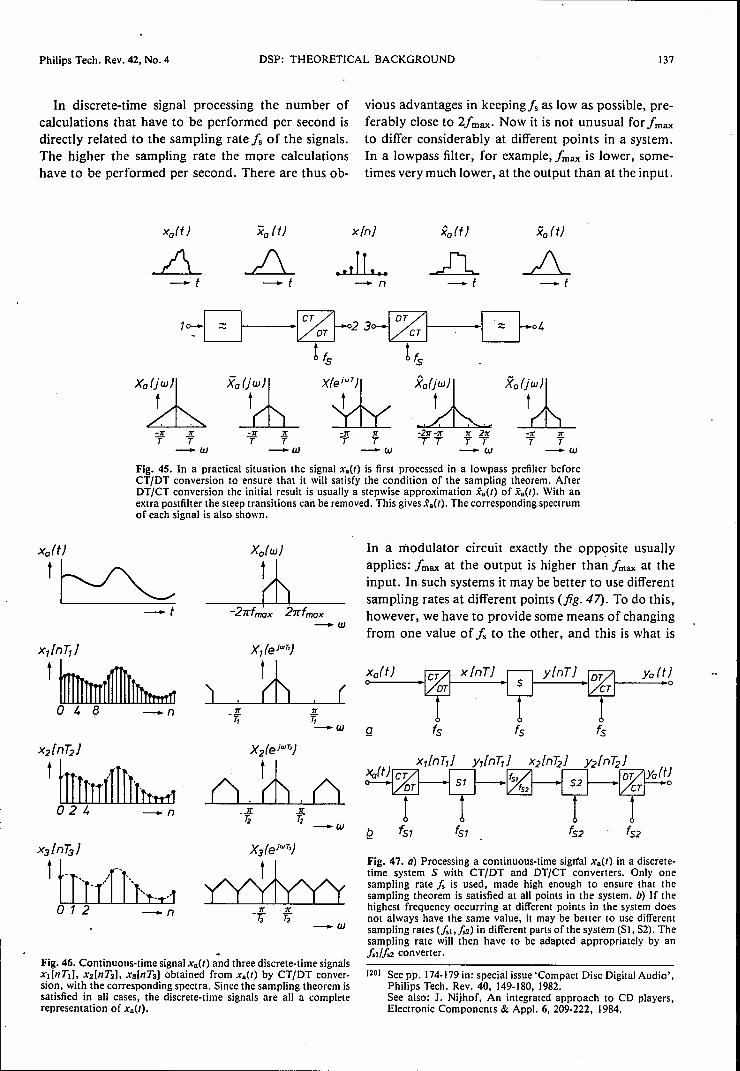
Philips Tech. Rev. 42, No. 4 OSP: THEORETICAL BACKGROUND 137
In discrete-time signal processing the number ofcalculations that have to be performed per second isdirectly related to the sampling rate Is of the signals.The higher the sampling rate the more calculationshave to be performed per second. There are thus ob-
Xa (t)
-t -t
vious advantages in keeping j', as low as possible, pre-ferably close to 2/max. Now it is not unusual for Imaxto differ considerably at different points in a system.In a lowpass filter, for example,/max is lower, some-times very much lower, at the output than at the input.
x ln]
."fL .. JL-t -t-n
D--ffi ~810-- 02 30-- . ::t: 04_ OT CT·
1,5 ltS
X"Ik X"~ x~ ~:!l_X"!h_-71: 71: -71: J!. -71: 7r -271:-71: 71: 271: -71: 71:T T T T T T TT TT Y T-w -w -w -w -w
Fig. 45. In a practical situation the signal x.{t) is first processed in a lowpass prefilter beforeCT/OT conversion to ensure that it will satisfy the condition of the sampling theorem. AfterOT/CT conversion the initial result is usually a stepwise approximation x.(1) of xa(1). With anextra postfilter the steep transitions can be removed. This gives x.(1). The corresponding spectrumof each signal is also shown.
xa(ti
l~-t
xtfn71J
l~o 4 8 --n 71:
f,"-w
X2/n]2J
llrrnrrrIIullhrrl024 -n 71:
Ti -w
X2(ejWT,)
(),~,{J
x3/nT3J
1hltTlh.x.l012 --n
-w
-Fig. 46. Continuous-time signal x.{t) and three discrete-time signalsxI[nTd, x2[nT21, xa[nTa) obtained from xa(t) by CT/OT conver-sion, with the corresponding spectra. Since the sampling theorem issatisfied in all cases, the discrete-time signals are all a completerepresentation of x.{t).
In a modulator circuit exactly the opposite usuallyapplies: Imax at the output is higher than Imax at theinput. In such systems it may be better to use differentsampling rates at different points (jig. 47). To do this,however, we have to provide some means of changingfrom one value of is to the other, and this is what is
xa(t) Ya (t)
(
Q fs tsfs
Fig. 47. a) Processing a continuous-rime sigrïal x.{t) in a discrete-time system S with CT/OT and OT/CT converters. Only onesampling rate j, is used, made high enough to ensure that thesampling theorem is satisfied at all points in the system. b) If thehighest frequency occurring at different points in the system doesnot always have the same value, it may be better to use differentsampling rates (!sI.!.2) in different parts ofthe system (SI, S2). Thesampling rate will then have to be adapted appropriately by an!sI/!s2 converter.
[201 See pp. 174-179 in: special issue 'Compact Disc Digital Audio',Philips Tech. Rev. 40, 149-180, 1982.See also: J. Nijhof, An integrated approach to CD players,Electronic Components & Appl. 6, 209-222, 1984.

138 A. W. M. VAN DEN ENDEN and N. A. M. VERHOECKX Philips Tech. Rev. 42, No. 4
Tt" ,-~.-,,,,
x[nT,J
t-n
y[n~J
to -n
r------- ----,I II I
x[nTtJ<>----+-1- IR II
I SRD!L ._. . _J
-7rT,
7rt;
14-----iFI
-w
• 0 y[n~J
"
x[nTtJ
t ,,,""'~-O":---1'__~2:---
,
_,
y[nTiJ 7it
.:......<-:--~-,, ,,, ,, ,,-, ,,
0 3 6 -n-n
,-----------,I :I I
X [ n TtJ o----t-i -, t R I
I I: SRI :L _
-w
.0 y[n~J
FI
Fig. 48. a) A circuit that decreases the sampling rate (SRD) by an integral factor!sI/f.2 = T2/T
1= R
eliminates R - I samples from every R input samples (here R = 3). b) A circuit that increases thesampling rate (SRI) by an integral factor !s2/fsl = T1/T2 = R adds R - I samples with the value 0between every two input samples (here R = 3). A schematic spectrum is shown for each signal.PI fundamental interval.
done in an !sd1s2 converter. We shall confine ourattention now to the cases in which the ratio !sI /!s2 or1s2/1s1 is an integer R. If!s2 < Isi we have a circuitthat decreases the sampling rate (SRD, for SamplingRate Decreaser) by a factor R, and if 1s2 >!sI we havea circuit that increases the sampling rate (SRI, forSampling Rate Increaser) by a factor R. We indicatethese circuits by the two special block-diagram sym-bols given in fig. 48. The operation of an SRD or anSRI can easily be pictured from the input and output
signals shown in this figure. With the SRD for every Rsuccessive input samples only one sample appears atthe output. All the SRI does is to add R - 1 sampleswith the value 0 between every two input samples. Inpractice operations of this kind can be implementedvery easily. But what happens to the overall operationof a discrete-time system when SRIs and SRDs areused? In answering here we must be careful to takethe following 'complication' into account: SRIs andSRDs do not come under the category of LTD sys-
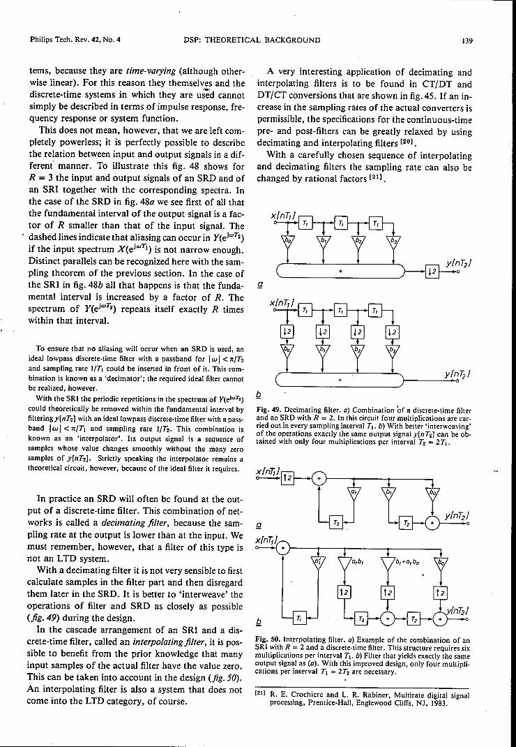
Philips Tech. Rev. 42, No. 4 DSP: THEORETICAL BACKGROUND 139
terns, because they are time-varying (although other-wise linear). For this reason they themselves and thediscrete-time systems in which they are used cannotsimply be described in terms of impulse response, fre-quency response or system function.
This does not mean, however, that we are left com-pletely powerless; it is perfectly possible to describethe relation between input and output signals in a dif-ferent manner. To illustrate this fig. 48 shows forR = 3 the input and output signals of an SRD and ofan SRI together with the corresponding spectra. Inthe case of the SRD in fig. 48a we see first of all thatthe fundamental interval of the output signal is a fac-tor of R smaller than that of the input signal. Thedashed lines indicate that aliasing can occur in Y(ejwT2)if the input spectrum X(ejwTI
) is not narrow enough.Distinct parallels can be recognized here with the sam-pling theorem of the previous section. In the case ofthe SRI in fig. 48b all that happens is that the funda-mental interval is increased by a factor of R. Thespectrum of Y(ejwT2) repeats itself exactly R timeswithin that interval.
To ensure that no aliasing will occur when an SRD is used, anideal lowpass discrete- time filter with a pass band for Ita I< nlT2and sampling rate IITI could be inserted in front of it. This com-bination is known as a 'decimator'; the required ideal filter cannotbe realized, however.
With the SRI the periodic repetitions in the spectrum of Y(eJwT2)could theoretically be removed within the fundamental interval byfiltering y[nT21 with an ideallowpass discrete-time filter with a pass-band Iw I< nlTI and sampling rate IIT2. This combination isknown as an 'interpolator'. Its output signal is a sequence ofsamples whose value changes smoothly without the many zerosamples of y[nT21. Strictly speaking the interpolator remains atheoretical circuit, however, because of the ideal filter it requires.
In practice an SRD will often be found at the out-put of a discrete-time filter. This combination of net-works is called a decimating filter, because the sam-pling rate at the output is lower than at the input. Wemust remember, however, that a filter of this type isnot an LTD system.
With a decimating filter it is not very sensible to firstcalculate samples in the filter part and then disregardthem later in the SRD. It is better to 'interweave' theoperations of filter and SRD as closely as possible(fig.49) during the design.
In the cascade arrangement of an SRI and a dis-crete-time filter, called an interpolating filter, it is pos-sible to benefit from the prior knowledge that manyinput samples of the actual filter have the value zero.This can be taken into account in the design (fig. Sa).An interpolating filter is also a system that does notcome into the LTD category, of course.
A very interesting application of decimating andinterpolating filters is to be found in CT/DT andDT/CT conversions that are shown in fig. 45. If an in-crease in the sampling rates of the actual converters ispermissible, the specifications for the continuous-timepre- and post-filters can be greatly relaxed by usingdecimating and interpolating filters [201.
With a carefully chosen sequence of interpolatingand decimating filters the sampling rate can also bechanged by rational factors [211.
g
y[n72J+
Fig. 49. Decimating filter. a) Combination of a discrete-time filterand an SRD with R = 2. In this circuit four multiplications are car-ried out in every sampling interval TI. b) With better 'interweaving'of the operations exactly the same output signal y[nT21 can be ob-tained with only four multiplications per interval T2 = 2TI•
Fig. 50. Interpolating filter. a) Example of the combination of anSRI with R = 2 and a discrete-time filter. This structure requires sixmultiplications per interval TI. b) Filter that yields exactly the sameoutput signal as (a). With this improved design, only four multipli-cations per interval Tl = 2T2 are necessary.
[21) R. E. Crochiere and L. R. Rabiner, Multirate digital signalprocessing, Prentice-Hall, Englewood Cliffs, NJ, 1983.

140 A. W. M. VAN DEN ENDEN and N. A. M. VERHOECKX Philips Tech. Rev. 42, No. 4
From continuous amplitude to discrete amplitude
As we saw at the beginning of this article, thesamples from which digital signals are built up canonly have discrete values. Indeed, the same is true ofall the other quantities (such as filter coefficients) thatoccur in digital systems.
'"g £Fig. SI. Three different quantization characteristics: a) roundingoff, b) value truncation, c) magnitude truncation. q quantizationstep.
g
Fig. 52. Three different overflow characteristics: a) saturation,b) zeroing, c) sawtooth overflow.
Table 11.Four examples of number representations commonly usedin digital signal processing. The word length B is put equal to 3 inall cases.
Decimal Sign and One's-com- Two's-com- Offsetvalue magnitude plement plement binary
+4 - - - III+3 011 011 011 110,+2 OIO OIO OIO 101+1 OOI OOI OOI 100+0 000 000 000 --0 100 III - 011-I 101 110 III OIO-2 110 101 110 OOI-3 III 100 101 000-4 - - 100 -
In practical applications of digital systems, how-ever, we often start with analog signals which, bydefinition, are continuous in amplitude. In dealingwith the theory of discrete-time systems so far wehave always assumed a continuous amplitude.The transition from continuous amplitude to dis-
crete amplitude is in principle never completely rever-sible, since the number of permitted values unavoid-
ably decreases. This means that there is always a lossof information, however slight. In this transition threeconcepts are crucial: quantization, overflow and num-ber representation. Let us first consider these threeconcepts.
Quantization
Quantization is the process in which a quantity x isconverted into a quantity xQ that is approximatelyequal to x but can assume fewer different values thanx. The relation between x and xQ is called the quan-tization characteristic. The most widely used forms ofquantization in digital processing are (fig. 51): round-ing off, value truncation and magnitude truncation.In these examples there is always ~ fixed distance q,the quantization step, between the successive discretevalues of xQ.
Overflow
Overflow is what happens when a quantity x seeksto assume a value outside the limits (-X, +X) thatmust be observed. In formal terms we can describethis as-a conversion of x into Xp, where
{-x
xp :::;Xlxi <xlxi> x. (80)
The relation between x and Xp is called the overflowcharacteristic. Three examples are given in fig. 52:saturation, zeroing and sawtooth overflow. In theory,any form of quantization can be combined with anyform of overflow; we can always form a combinedoverflowjquantization ch-aracteristic.
Number representation
Usually the value of a quantity in a digital system is"expressed as a group (a 'word') of a specified number(say B) of bits. The corresponding overflowjquantiza-tion characteristic then has a maximum of 2B differentvalues. Each of these values corresponds to one par-ticular group of B bits. Which particular group it isdepends on the number representation used. There isconsiderable variety in this. By way of illustration,four common number representations for B = 3 aregiven in Table11. Some forms of quantization or over-flow go better with one form of representation thanwith anothe~. In practice there are distinct preferencesfor particular combinations.The fact that binary words in digital systems always
have a finite length results in a number of effects thatwe shalliook at in more detail in the next section.
Before going on we should perhaps note that thecommon concept of analog-to-digital conversion(often abbreviated to AID conversion) includes thecombination of the CTjDT conversion from the sec-

Philips Tech. Rev. 42, No. 4 DSP: THEORETICAL BACKGROUND 141
ti on headed 'From continuous time to discrete timeand vice versa' and the conversion from continuousamplitude to discrete amplitude dealt with in this sec-tion.
Finite-word-length effects
In this section we shall look at three situations inwhich the finite word length is a significant factor.These are AID conversion, digital filter design and theexecution of digital computations.
AIDconversion
In converting a signalof continuous amplitude x[n)into a signalof discrete amplitude xQ[n), we can pro-ceed as if xQ[n) were obtained by adding the noisy sig-nal e[n) = xQ[n) - x[n) to x[n) (fig. 53). In this waywe arrive at the useful concept of quantization noise.If we now consider specifically the case of quantiza-tion by rounding off with step size q, the power P, ofthis noise is given by:
q2r, = 12
If we then also assume that the samples of xQ[n) arerepresented as words of B bits and that x[n) is a sinus-oidal signal with the largest possible amplitude beforeoverflow can occur, we then find a signal! quantizationnoise ratio of
Px = 6B + 1.76 (dB)Pe
inxQ[n). An important conclusion of generally validitycan be drawn from this equation: any increase of theword length B by one bit improves the maximumachievable signal/quantization noise ratio by 6 dB.
Digital filter design
The procedures described earlier for designing dis-crete filters generally give very accurate values for thefilter coefficients. In a practical digital filter, however,the number of bits used for representing the coeffi-cients must be as small as possible, largely for reasonsof cost. The values found must therefore be quan-tized. But this alters the characteristics of the filter [22],
i.e. it changes the locations of the poles and zeros.These changes can be very substantial (fig. 54). It mayhappen that, after quantization, the filter no longersatisfies the design specifications that were used in cal-culating the unquantized coefficients. In extreme casesa stable filter may even become unstable, because apole moves from a position inside the unit circle inthe z-plane to a position outside it. However, thequantization of filter coefficients introduces no changes
in the linear operation of a circuit, nor does it causeany effects that depend on the input signalor that varywith time. It introduces no more than a once-only cal-'culable change in the characteristics of the filter.
Some filter structures are much more sensitive toquantization of the coefficients than others. In generala filter structure becomes less sensitive as the locationof each pole and each zero becomes dependent onfewer coefficients. This point has been mentionedbriefly in the section 'Discrete filter structures'.
Another significant effect is that the possible posi-tions for poles and zeros with quantized coefficientsdo not have to be uniformly distributed over the z-plane. This can vary considerably with the structureof the filter. If poles and zeros are required in regionswhere there are few, the quantization effects will bemore pronounced. This is illustrated in fig. 55, whichshows two simple purely recursive filters of the 2ndorder, with the possible pole positions when the coeffi-cients are quantized to four bits (one of them for thesign). Because of the symmetry only one quadrant o~the z-plane is shown.
(81)
xf!!!_~n]~~o
-n -nQ
(82) xInl ~]~~o
tefn]
et~~~L':£i~_"-q -n
Fig. 53. a) Conversion of a signalof continuous amplitude x[n) intoa signalof discrete amplitude xQ[n) can be regarded as the additionof a noisy signal ern) = xQ[n) - x[n). b) Equivalent circuit basedon this.
-8o 7r12OdB~--------~~----------~
-5020 log A (eiB)
1-100
Fig. 54. Amplitude characteristic of a transversal filter (of lengthN = 49) with unquantized coefficients (continuous line) and coeffi-cients rounded off to 12 bits (dashed line).
[22) V. B. Lawrence and A. C. Salazar, Finite precision design oflinear-phase FIR filters, Bell Syst. Tech. J. 59, 1575-1598,1980.

142 A. W. M. VAN DEN ENDEN and N. A. M. VERHOECKX Philips Tech. Rev. 42, No. 4
Digital computations
The most complicated consequences of working witha finite word length are found when limiting the wordlength of intermediate results in digital systems [231.
Just as in everyday calculations in the decimal system,addition and multiplication in the binary system oftenincrease the number of digits required, i.e. the wordlength. With recursive filters, however, this inevitablyintroduces problems because the result of one calcula-tion is the starting point of the next. See for examplefig. 55a: ify[n] and the coefficient as both have a wordlength of 4 bits, this can give a result of 7 bits aftermultiplication. Calculation of the next input sample
Q
speaking the filter is not linear. The most troublesomeeffects are usually due to overflow: signal distortioncan then be very serious, and with recursive structuresthere may even be 'overflow oscillations' of very largeamplitude. Filters are therefore generally designed sothat this cannot happen or only happens very rarely.A widely used aid in this context is 'sealing', particu-larly for filters consisting of cascaded sections. In thedesign a multiplier by a constant factor « 1) is in-serted between the sections, to prevent the occurrenceof overflow in the following section. If this factor isan integral negative power of 2, the multiplicationonly means a shift of the sample value by one or more
yln]
1 -T--r-,-...Im z -+-+-+~>,
I I I I -,
t -+-+-+-+--h-+-+-+-+-+-+1 1 1 1 1 1\
05 -+-+-+-+-+-+-~1 1 1 1 1 1 1\-+-+-+-+-+-+--t-\1 1 1 1 1 1 1 \-+-+-+-+-+-+-+-11 1 1 1 1 1 1 \-+-+-+-+-+-+-+-~1 1 1 1 1 1 1 I
00 05 1-r+Re s:
....._-----<:-b,f-------'
Fig. SS. 0) Purely recursive 2nd-order filter with direct-form structure and realizable complexpoles when the value of the filter coefficients al and 02 is expressed in terms of four bits (one bit isfor the sign). Because of the symmetry, only one quadrant of the z-plane is shown. b) Purely re-cursive znd-order filter with coupled structure. In this structure the positions of the realizablecomplex poles are distributed quite differently over the z-plane for the same quantized coefficientvalues. .
can then give an intermediate result of more bitsagain, then more again, and so on.
With recursive structures we are therefore forced to
limit the word length of intermediate results. Withnon-recursive filters the increase in the word length isalways finite, but even then some limitation may oftenbe necessary. In principle we can still choose the formof quantization and overflow (or both) to be used, andwhether it should be used at one or more places in thefilter. This can have completely different effects on theoperation of the filter.
The great problem in analysing word-length limita-tion of intermediate results rests in the fact that strictly
binary places. (In some cases scaling by a constant> 1 will be used, if it appears during the design thatthe most significant bits in the following section wouldotherwise remain unused.) After such measures havebeen taken, overflow does not have to be consideredfurther. Then an attempt is usually made to get someidea of the effects due to quantization of the inter-mediate results in the filter output signal.In the first place this gives rise to an unwanted
'noisy' signal, rather like the quantization noise inAID conversion. This noise is generated at the quan-tizers and is filtered ('coloured') on its way to the out-put of the filter. To obtain quantitative results the

Philips Tech. Rev. 42, No. 4 DSP: THEORETICAL BACKGROUND 143
occurrence of this quantization noise is modelled inthe same way as with AID conversion: each quantizeris replaced by an additive noise source (fig. 56). Theassumption is made that each source produces noisewith a particular frequency spectrum (in the case of
Q
we assume that x[n] = 0 for n > 0 and y[O] = 7q, wesee that oscillations of period N = 2 and amplitude 5qappear in the output signal.
In recursive filter sections of higher order, limitcycles are a familiar problem, and they have to be
~e:?f( +
Fig. 56. a) Example of a digital filter in which the word length of the intermediate results is limitedby the quantizers Ql,"" Qs after each multiplication. b) To obtain an idea ofthe noise then pro-duced in the output signal yIn), a noise-source model is used: each quantizer is replaced by animaginary additive noise source eJ[n], ... , es[n). If quantization is by rounding off with step sizeq, each source has a noise power of q2/12 and a flat ('white') spectrum. The noise is then filteredwith the frequency response encountered between a particular source and the output. In the filtershown here the noise contributions of e3[n), e4[n) and e5[n) appear unfiltered at the output. Thecontributions from eJ[n) and e2[n), on the other hand, are filtered in the same way as the inputsignal x[n].
rounding off, the noise has a flat spectrum and a totalpower of q2/12). The noise contribution at the outputof the filter from each source can then be calculated.Although this analysis with noise sources can pro-
duce very useful results, it is based on a number ofassumptions that are usually not entirely correct andcan sometimes even be quite wrong. This applies forexample to the assumption that the noise contribu-tions are independent of each other and independentof the useful signals in the filter. Provided the wave-form of the input signal x[n] is sufficiently irregular,the assumption is not unreasonable. This situationchanges, however, if the value of the input signal isconstant (or zero) over a longer period of time or isperiodic. Periodic interference signals ('limit cycles')may then appear at the output. If for example x[n] is adigitized speech signal, this may happen in the pausesin the conversation. But this is where periodic inter-fering signals, even at a very low level, are most annoy-ing. A very simple example is shown in fig. 57, wherethe intermediate result is quantized by rounding off. If
x~Y{n}+ 10
WQ{~
n wlnl=-O.91yln-1l ylnl=wQlnl0 ... 7q1 -6.37q -6q2 5.1.6q 5q3 -1..55q -5qI. 4.55q 5q5 -1..55q -5q... ... ...... ... ...
Fig. 57. In this simple model a limit cycle of period N = 2 andamplitude 5q arises when x[n) = 0 for n > 0 and y[O) = 7q. Inquantizer Q there is rounding off with step size q.
(23) T. A. C. M. Claasen, W. F. G. Mecklenbräuker and J. B. H.Peek, Effects of quantization and overflow in recursive digitalfilters, IEEE Trans. ASSP-24, 517-529, 1976.
144 DSP: THEORETICAL BACKGROUND Philips Tech. Rev. 42, No. 4I.
taken into account. It is found that quantization bymeans of magnitude truncation is not so liable tocause oscillation of this type as other forms of quan-tization. It is also useful to know that limit cycles arealways confined to a number of the least significantbits. If we reduce the quantization step q of all thequantizers in a filter in which these cycles occur by in-creasing all the word lengths, then the amplitude ofthe limit cycle expressed in an absolute sense (e.g. as avoltage and not as a number of quantization steps)will also decrease. By then quantizing the outputsignal yen] we can make a filter that is apparently freefrom limit cycles.
Summary. In the theoretical aspects digital signal processinghastwo essential characteristics: all the processes take place in discretetime and all the quantities occurring in the processes are discrete inamplitude, i.e. they can only assume discrete values. Theoreticalanalyses relating to discrete time require special techniques, such asthe Fourier transform for discrete signals (FTD), the z-transform(ZT), the discrete Fourier transform (DFT), the fast Fourier trans-form (FFT) and the use of difference equations, where the discrete-amplitude aspect is deliberately left out of consideration. With thisapproach, many parallels can be found between analog signal andsystem theory on the one hand and digital signal and system theoryon the other. This means that existing analog design techniques(e.g. for filters) can be used as the starting point for the design ofdigital filters and systems. The transition from continuous time todiscrete time and from continuous amplitude to discrete amplitudehas much to offer (new system structures, changing of sampling .rate) but also raises new problems (aliasing, instabilities, quantiza-tion noise). These problems form a separate branch of the theory ofdigital signal processing.
.~.;:.... ... J.~
, ..
.."' ....
--~'._""'!"'-:' ..
... 10
to.. t.: ~. '!' "-


![xidexia@bu.edu Zijun Huang Columbia University arXiv:1812 ... · Dataset Year Images Classes Domains Description Digit-Five - ˘100,000 10 5 digit Office [37] 2010 4,110 31 3 office](https://static.fdocuments.us/doc/165x107/5eb53f6820c55033793d5221/xidexiabuedu-zijun-huang-columbia-university-arxiv1812-dataset-year-images.jpg)