Digital Signal Processing- -...

Digital Signal Processing-Basic Concepts

Some materials from Dr. Larry Marple are acknowledged

Outline

Background materialsContinuous-time signals and transformsFourier transform and propertiesSampling and windowing operationsDiscrete-time signals and transforms

display

B, M, Doppler image

processingDoppler

processing

digital receive beamformer

system controlkeyboard

beamformercontrol

digital transmit beamformer DAC

high voltage

amplifier

ADCvariable

gain

T/R switch

arraybody

All digital

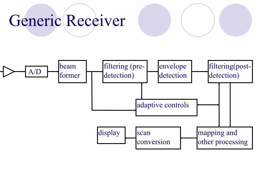
beam former

filtering (pre-detection)

envelope detection

filtering(post-detection)

mapping and other processing

scan conversion

display

adaptive controls

A/D

Generic Receiver

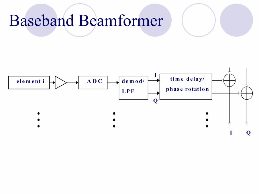
e l em ent i A D C dem od/

LPF

tim e de lay/

phas e rotati o n

I Q

I

Q

Baseband Beamformer

CW oscillator

PW transmitter (gated CW)

transducer amplifier

demod./LPF

filter spectral estimation

audio conversion

displayspeaker

signal processing

gating

sample&hold

PW Doppler

DSP Building Blocks in Imaging

FilterModulator/demodulatorDecimator/interpolatorFourier transformerHilbert transformerDetectorAutocorrelatorBeamformer

Hierarchy of Signal & System Properties

StochasticDeterministic

Time-invariant

Time-varying

Nonlinear

Linear

Temporal & Spatial Signal Distinction

Continuous-time (CT) signalsContinuous-space (CS) signals

Analog signalsDiscrete-time (DT) signalsDiscrete-space (DS) signals

Sampled-data signals (typically uniform sampling)Digital signals: DT or DS signals with quantized ampltitudes

Main Approach

All DT (DS) DSP theory is derived from the CT (CS) signal processing theory.Sampling scheme: one value per sampling point.Sampling scheme: uniform temporal (spatial) sampling intervals (will introduce periodicity).

[ ][ ] (m) interval Sampling: )(

(sec) interval Sampling: )(DmDxmy

TnTxnx==

Signal Representation Domains

t (time, sec) f (temporal frequency, cycles/sec=Hertz)d (space, m) k (spatial frequency, wavenumber, cycles/meter) or λ=1/k (wavelength, meters/cycle)(t, d) (propagating waves, coupled time and space signal) (f, k) Coupled frequencies (k=f/c)

Acoustic Wave Equations

∂∂

ρ ∂∂

2

2

2

2

w z t

tB

w z t

z

( , )( / )

( , )=

w z w e w ej z c j z c( , ) ( ) ( )/ /ω ω ωω ω= +−1 2

w z t w t z c w t z c( , ) ( / ) ( / )= − + +1 2

Complex Numbers and Complex Arithmetic

Required to define roots of polynomials:

Required to define solutions of linear differential (difference) equations:

012 =+z

0)()(2

2

=+ sXds

sXd

Complex Addition and Subtraction

[ ] [ ] [ ][ ] [ ] [ ]BABA

BABAImImImReReRe

±=±±=±

Complex Conjugate

222*

*

AaaAA

ajaAA

ajaAA

ir

ira

ira

=+=⋅

⋅−=−∠≡

⋅+=∠=

φ

φ

Complex Multiplication

[ ] [ ]]Im[]Im[],Re[]Re[ real, is if

ImRe)()(BkkBBkkBk

ABABbabajbabaBA riiriirr

==+=−⋅+−=⋅

Complex Division (Rationalization)

2222*

*

ir

riir

ir

iirr

aaababj

aaabab

AABA

AB

+−

+++

==

Complex Number in Exponential Form

Euler’s formula: Complex number in exponential form:

ααα sincos jje ±=±

ajeAAφ

=

0901∠=

−∠=

+∠=⋅

j

BA

BA

BABA

ba

ba

φφ

φφ

Complex Signals

Signals represented as a pair of linked real-valued signals:

{ }

(Q)component phase-quadratureor part imaginary :)((I)component phase-inor part real:)(

)()()(),()(

tyty

tyjtytytyty

i

r

irir ⋅+==

Complex Numbers in the Complex Plane

ai

ar

Aa

Aa

φ

φ

sin

cos

=

=

1−≡j

Rotating phasor

( )

0 tan180

0 tan

10

1

2/122

<

−±=

>

=

+=

−

−

rr

ia

rr

ia

ir

aaa

aaa

aaA

φ

φI/Q signals are 90o out of phase

))(cos()90)(sin( 0 tt θθ =+

Complex SignalsCreated from real-valued signals by operations such as

Complex modulation/demodulation (aka quadraturemodulation)Fourier transformationComplex filteringBaseband signal generation from memory

AdvantagesSimplifies mathematical analysisReduce hardware data ratesReduces arithmetic and filtering requirements for

modulation/demodulation/phase adjustment

Advantage of Complex Representation: Modulation as an Example

[ ]

[ ] ( ) ( )[ ])()(cos)()(cos)()(21)()(

)(cos)()( ),(cos)()(

)()()()(

)()( ,)()(

21212121

222111

)()(2121

)(22

)(11

21

21

tttttatatxtx

ttatxttatxor

etatatxtx

etatxetatxtt

tt

θθθθ

θθ

θθ

θθ

++−⋅=⋅

⋅=⋅=

⋅=⋅

⋅=⋅=+

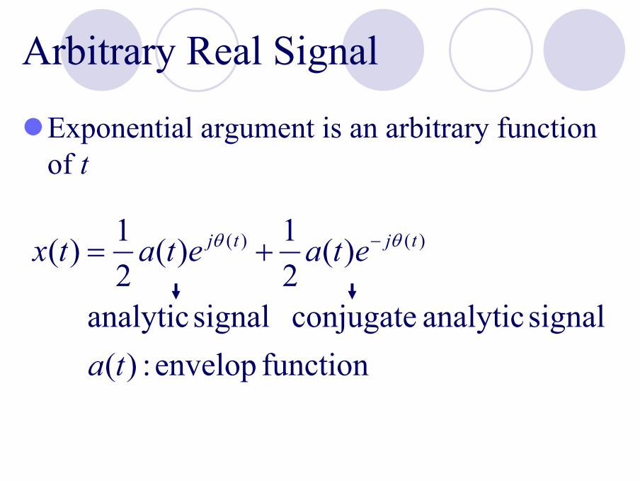
Arbitrary Real Signal

Exponential argument is an arbitrary function of t

function envelop :)( signal analytic conjugate signal analytic

)(21)(

21)( )()(

ta

etaetatx tjtj θθ −+=

Do Negative Frequencies Exist?

Continuous-Time Signals and Transforms

Continuous-Time System Response

Consider responses to the following inputsComplex exponential signalComplex sinusoidal signalModulated Gaussian signalImpulse function (limit of Gaussian signals)

h(t)x(t) y(t)

)()()()(

)()()()()(

thtxtxth

dxthdtxhty

∗=∗=

−=−= ∫∫∞

∞−

∞

∞−ττττττ

Continuous-Time System Response to Complex Exponential

Motivation for Laplace transform

exists integral where and limitsfor )( of transformLaplace theis )( where

),()()(

,)(Let )(

sthsH

sHedehty

jsetxt stts

st

∫ ∞−

− ==

+==

ττ

ωστ

est is an eigenfunction of the LTI CT systemH(s) is the continuous-time system function

Continuous-Time System Response to Complex Sinusoidal Signal

Motivation for Fourier Transform

)( of ansformFourier tr theis )( where

)()()(

sincos)(,0Let

-

thH

dehHjsH

tjteetxjsj

tjst

ω

ττωω

ωωωωτ

ω

∫∞

∞

−===

+===+=

Fourier transform of the system temporal function is the system response function to input complex sinusoidal signals

{ }tethFTLT σ)(=

Gaussian Signals

Unmodulated Gaussian Signal (the transform is also Gaussian)

2222

)()( / TfTt TefGetg ππ −− =⇔=Modulated Gaussian Signal (with complex sinusoid)

22)(

2 )()()()()(Tff

ctfj

c

c

ATe

ffAfGfXAetgtx−−=

−∗=⇔=π

π δ

Body Ultrasound Attenuation Filter

I(z) I(z+∆z)

z z+∆z

A

A I z z A I z A I z z⋅ + = ⋅ − ⋅( ) ( ) ( )∆ ∆2β

− = ⋅

= −

∂∂

β

β

I z

zI z

I z I e z

( )( )

( )

2

02

β α= f

Frequency domain attenuation response


H z f e fz j fz c( , ) ( / )= − +α π2

I z f I H z f I e fz( , ) ( , )= = −0

2

02α


Assuming a Gaussian signal:

S f et

f f

( )( )2

0 2

=−

−σ

S R f S f e er tRf

f fRf

( , ) ( )( )2 2 4

40 2

= =−−

−−α σ

α

S R f e er

f fR f R

( , )( )

( )2 41 2

02

=−

−− −σ α σ α

f f R1 022= − σ α .

0R2R

f

Impulse Function

Introduced in 1947 by DiracUseful signal processing tool for

Sampling operationsRepresenting the transform of sinusoidal signals

Impulse is a brief intense unit-area pulse that exists conceptually at a point

1)( =∫∞

∞−dttδ

Impulse Function

Visualize as a limiting sequence of a window function, such as a Gaussian window

∫∞

∞−

−

→=1)(lim 1

0dttgT

T

g(t)

g(t) G(ω)

lim lim

Impulse Function

PropertiesProduct

Convolution

Convolution with an impulse results in a shift operation

)()()()()()0()()(

τδττδδδ

−=−=

txttxtxttx

)()()()()()(

ττδδ

−=−∗=∗

txttxtxttx

Continuous-Time System Response to Impulse Function

Thus, h(t) has the interpretation as the impulse response of the continuous-time system (filter).

∫ ∞−=−=

=t

thdthty

ttx

)()()()(

)()(Let

ττδτ

δ

Fourier Transform and Properties

The Fourier Transform

Forward Fourier transform (generally complex-valued)

Reverse (backward) Fourier transform

Base Fourier transform from which all other Fourier transform variations are derived.

{ } ∫∞

∞−

−== dtetxXtxFT tjωω )()()(

{ } ∫∞

∞−

− == ωωω ω deXtxXFT tj)()()(1

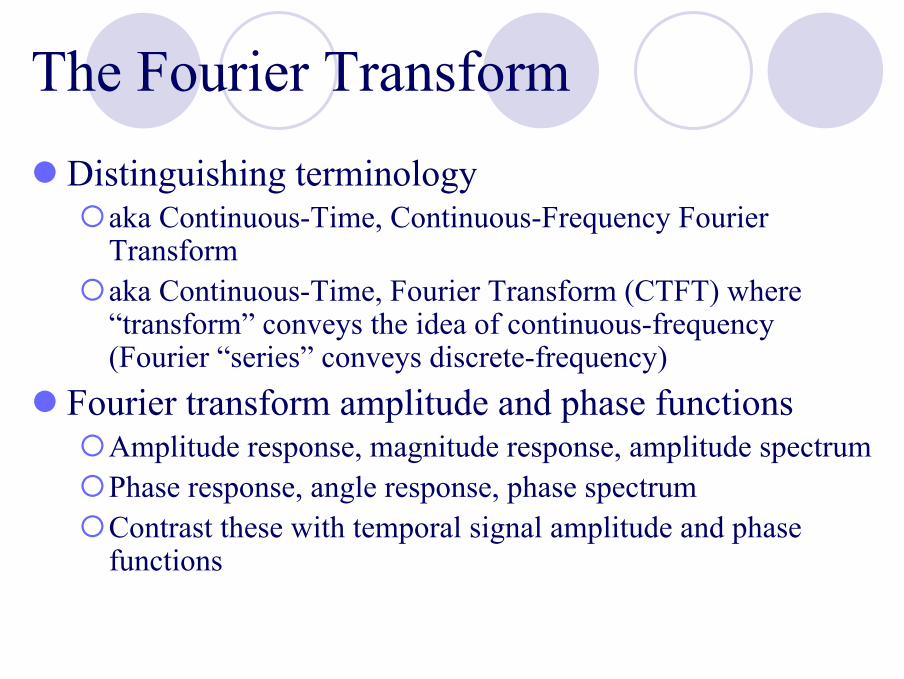
The Fourier TransformDistinguishing terminology

aka Continuous-Time, Continuous-Frequency Fourier Transformaka Continuous-Time, Fourier Transform (CTFT) where “transform” conveys the idea of continuous-frequency (Fourier “series” conveys discrete-frequency)

Fourier transform amplitude and phase functionsAmplitude response, magnitude response, amplitude spectrumPhase response, angle response, phase spectrumContrast these with temporal signal amplitude and phase functions

Even-Odd Signal Decomposition and Fourier Transform Properties

Any function can be separated into even and odd components:

Transform

[ ] [ ])()(21)(,)()(

21)( where

)()()(

txtxtxtxtxtx

txtxtx

oddeven

oddeven

−−=−+=

+=

)()()( ωωω oddeven XXX +=

Even-Odd Signal Decomposition and Fourier Transform Properties

{ } { } { } { }

{ } { } { } { })(Im)(Re)(Im)(Re)(

)(Im)(Re)(Im)(Re)(

ωωωωω oddoddeveneven

oddoddeveneven

XjXXjXX

txjtxtxjtxtx

+++=

+++=

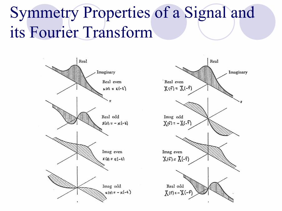
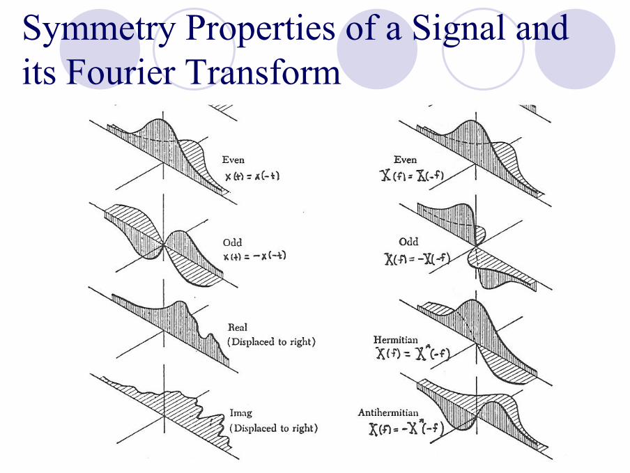
Symmetry Properties of a Signal and its Fourier Transform

Visualizing the System Response

The Logarithmic Scale

Definition of decibel (dB)

If P=V2/R

)/(log10 10 refPPdB =

)/(log20)/(log10 1022

10 refref VVVVdB ==

Summary of Key CTFT Properties and Functions

Special Signals and Their Transforms

Cosine signal

Time-domain window function (akarectangular window)

tfjtfjc

cc eetftx πππ 22

21

212cos)( −+==

tttcTfcT

TtTt

TttT π

πsin)(sin),2(sin22/,02/,2/1

2/,1)( =⇔

>=

<=Π

X(f)

+fc-fc

T/2-T/2

X(f)

1/T-1/T

Special Signals and Their Transforms

Frequency-domain window function

F/2-F/2

1/F-1/F )()2(sin2 fFtcF FΠ⇔

Sign Function

Will be useful to develop the Hilbert transform

fjfX

ttt

ttxπ−

=⇔

<−=>

== )(0,1

0,00,1

)sgn()(

Impulse Train

Infinite periodic sequence of impulse functions spaced T seconds apart

Transform is another impulse train

∑∞

−∞=

−n

nTt )(δ

-2T-3T -T 0 T 2T 3T

-2F-3F -F 0 F 2F 3F

1

F=1/T

∑∞

−∞=

−m T

mfT

)(1 δ

Impulse Train

Properties:Product: In this case, the impulse train is called a sampling function.

Convolution: In this case, the impulse train is called a replicating function.

∑∞

−∞=

−n

nTtnTx )()( δ

∑∞

−∞=

−m

mTtx )(

Graphical Illustration of Sequence of Impulse Functions

Energy Preservation Between Domains

Parseval-Rayleigh theorem

Energy theorem (let x(t)=y(t))

Energy spectral density

∫∫∞

∞−

∗∞

∞−

∗ = dffYfXdttytx )()()()(

energydffXdttxE === ∫∫∞

∞−

∞

∞−

22 )()(

2)( fX

Matched Filter

Objective: Determine system (filter) response h(t) that maximizes the output energy of the system responses for the given input signal (assuming max is reached by time t=t0).

Based on Schwarz inequality{ }∫ ∞−

−=−= 0 )()()()()( 100

tfHfXFTdttthtxty

∫∞

∞−

∗∗

⋅=

−==

dffHEty

ttcxthfcXfH22

0

0

)()(

)()(or )()(

Matched Filter

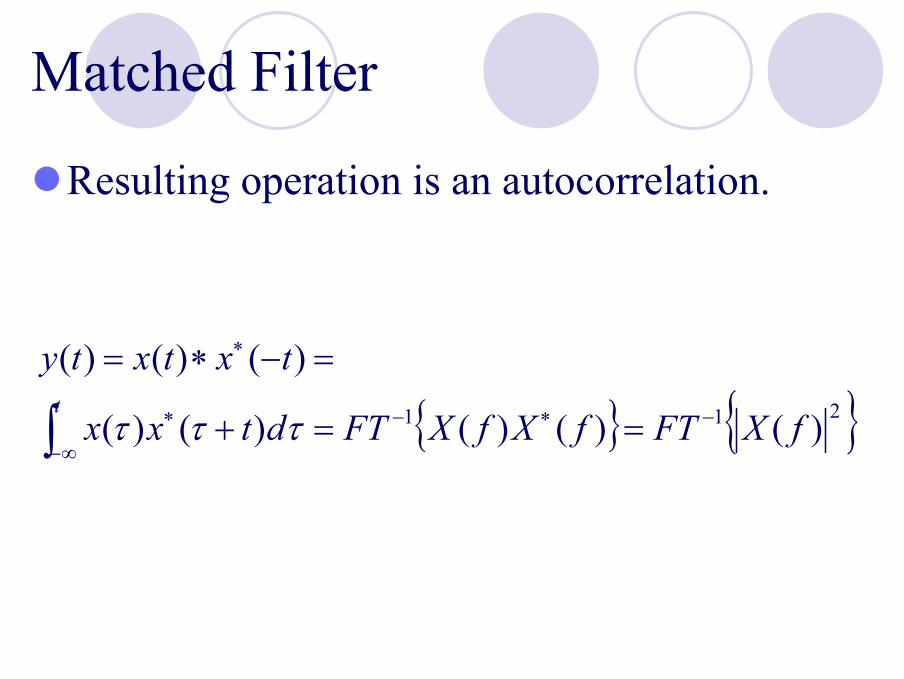
Resulting operation is an autocorrelation.

{ } { }211 )()()()()(

)()()(

fXFTfXfXFTdtxx

txtxtyt −

∞−

∗−∗

∗

==+

=−∗=

∫ τττ

Matched Filter and SNR

Assume the noise input to the filter (XN(f)) is uncorrelated with the filter and has frequency independent distribution as a function of frequency. We have

The output noise power becomes

X f NN ( )2

0≡

dtthNdffHNdffHfX N ∫∫∫∞

∞−

∞

∞−

∞

∞−=== 2

0

2

022 )()()()(σ

Matched Filter and SNR

When using the matched filter

The maximum signal-to-noise ratio is determined only by its total energy E, not by the detailed structure of the signal.

00

2

0

02

max

)()(

NE

N

dttx

N

dtttxSNR ≡=

−= ∫∫

∞

∞−

∞

∞−

Time-Bandwidth Product

Approach using the area metric

Rule of thumb: bandwidth of the pulsed signal is roughly the reciprocal of the signal’s time duration.

1

)0(/)(

)0(/)(

=⋅

=

=

∫∫∞

∞−

∞

∞−

βα

β

α

XdffX

xdttx

Time-Bandwidth Product

Approach using the variance metric

Equality when x(t) is Gaussian.Other metrics may be required to handle special cases (e.g., bandpass signals with no content near DC).

constant a

/)(4

/)(4

2222

2222

≥⋅

=

=

∫∫∞

∞−

∞

∞−

βα

πβ

πα

EdffXf

Edttxt

Range and Velocity Accuracy in Doppler Estimation

Let

With a matched filter, we have (the maximum occurs at t=0)

With noise, the maximum may shift to ∆t. Our goal is to derive < ∆t2 >

x t x t n t( ) ( ) ( )= +0

h t x t( ) ( )= −0

y t x x t d n x t d y t n x t d( ) ( ) ( ) ( ) ( ) ( ) ( ) ( )= − + − ≡ + −−∞

∞

−∞

∞

−∞

∞

∫ ∫ ∫0 0 0 0 0τ τ τ τ τ τ τ τ τ


Taylor expansion

We havey t y

ty R0 0

2

002

0( ) ( ) ( )∆∆

= + ′′ +

y t y t y E R0

2

0

2 200 0( ) ( ) ( )∆ ∆= + ′′ +

y t y E t02

02 2 2 20( ) ( )∆ ∆− = −β

′′ = ′′ −−∞

∞

∫y t x t x d0 0 0( ) ( ) ( )τ τ τ

′′ = ′′ = −−∞

∞

−∞

∞ ∗

∫ ∫y x x d f X f X f df0 0 02 2

0 00 4( ) ( ) ( ) ( ) ( )τ τ τ π

βπ π

2

2 20 0

0 0

2 20 04 4

≡ =−∞

∞ ∗

∗

−∞

∞−∞

∞ ∗

∫∫

∫f X f X f df

X f X f df

f X f X f df

E

( ) ( )

( ) ( )

( ) ( )

′′ = −y E020( ) β


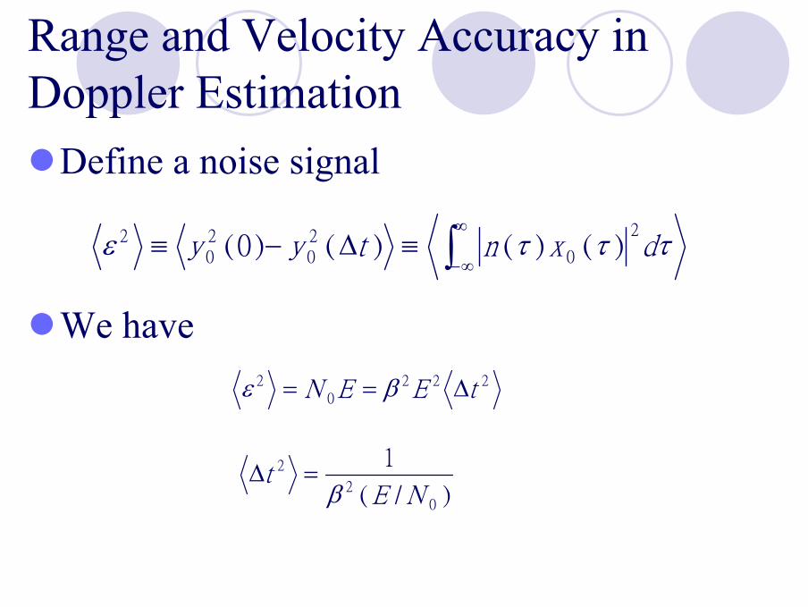
Define a noise signal

We have

ε τ τ τ202

02

0

20≡ − ≡

−∞

∞

∫y y t n x d( ) ( ) ( ) ( )∆

ε β20

2 2 2= =N E E t∆

∆tE N

2

20

1=β ( / )


Similarly

Thus

Gaussian signals give poorer simultaneous measurements of time and frequency than any other signal.

∆fE N

2

20

1=α ( / )

[ ]∆ ∆t fE N

2 21 2

0

1/

( / )=αβ

Essentially Time-Limited and Band-Limited Signals

Signals cannot be simultaneously band-limited and time-limited.Important for discrete-time applications that signal be band-limited (for sampling) and also for pulses to be time-limited (finite memory)

Essentially Time-Limited and Band-Limited Signals

Essentially time-limited

Essentially band-limited

f

T

T

ftjTL dtetxfXfXfX επ ≤−=− ∫−

−22/

2/

22 )()()()(

t

B

B

ftjBL dfefXtxtxtx επ ≤−=− ∫−

22/

2/

22 )()()()(

Analytic and Causal Signals

Causal and analytic signals are dual scenarios that link I/Q components through a Hilbert transformCausal signal is a signal that is 0 over negative time.Analytic signal is a complex signal with a transform that is 0 over negative frequency; created from a real signal.

Analytic and Causal Signals

Causal signal

Analytic signal

[ ]

ffjXfX

fjffXfX

ttxtxtxtx

eee

eoe

ππδ 1)()(1)()()(

)sgn(1)()()()(

∗−=

−∗=

+=+=

[ ])sgn(1)()(

1)()(1)()()(

ffXfXt

tjxtxt

jttxtx

a

a

+=

∗−=

−∗=

ππδ

Hilbert Transform

Transforms time time or frequency frequency

{ } ∫∞

∞− −=∗−= τ

ττ

ππd

tx

ttxtxHT

)()(11)()(

Sampling and Windowing Operations

Frequency Definitions

Signal frequencyF (units of cycles per second, Hz)

Sampling rateF=1/T, T is sampling interval in seconds (per sample)Units of samples per second

Fraction of sampling ratef/F=fT, dimensionless ratio (or cycles per sample)Bounded by +/- 0.5 (normalized frequency)

Band-Limited Transform Definitions for Continuous-Time Signals

Baseband (lowpass) real signal

Real bandpass signal

Complex signal of one-sided baseband real signal

Compex signal of one-sided bandpass real signal

Baseband complex signal

f

f

f

f

f

B

Creating One-Sided Complex LowpassSignals from Real Lowpass Signals

Analytic lowpass signalTime-domain approach

Frequency-domain approach

Delay

HT FIlter

x(t) xr(t)

xi(t)

Zero out -fx(t) {xr(t), xi(t)}IFTFT

Creating Baseband Complex Signals from Real Bandpass SignalComplex demodulation (quadratic demodulation)

Original

Band-shift

Low pass filter

Implementation

Four Basic Sampling and Windowing Operations Linking CT and DT Signals

Time sampling:Creates discrete-time signal (i.e., a time series)

Frequency windowing:Creates frequency-limited (i.e., band-limited) signal

Frequency sampling:Creates discrete frequency transform (i.e., a Fourier series)

Time windowing:Creates time-limited signal

Time Sampling Operation

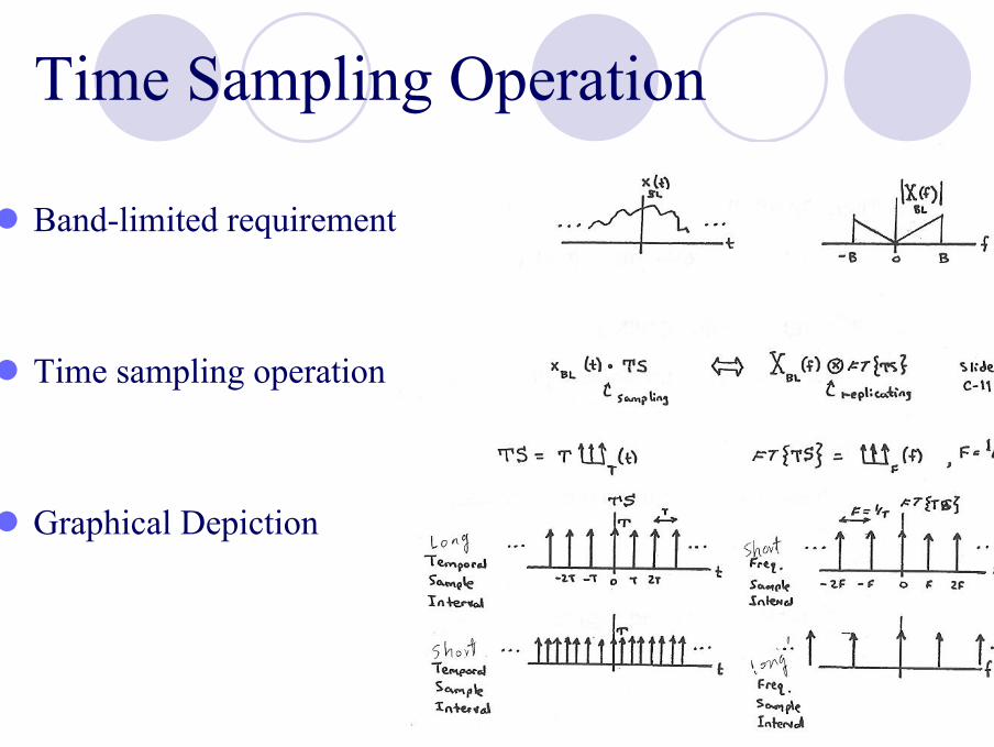
Band-limited requirement

Time sampling operation

Graphical Depiction

Selecting the Sampling Rate

Real baseband caseComplex baseband caseReal bandpass case

Sampling Real Baseband Signals

Case 1

Case 2

Case 3

BT

21

>

BT

21

<

BT

21

=

∑∑∞

−∞=

∞

−∞=

−⇔−=⋅=k

BLn

BLBLTS kFfXnTtnTxTTStxtx )()()()()( δ

Strictly Band-Limited Signals Do Not Exist in Practice

Some degree of aliasing cannot be avoided in actual hardwareAnalog anti-aliasing filters are imperfectAnalog-to-digital converters introduce digitization noise

Select sample rate based on bandwidth at which the signal is essentially band-limited.

Sampling Complex Baseband Signals

Signal and transform

Case 1

Case 2

Minimum sampling rate for complex baseband signal: F=B.

BT

21

=

BT 1=

Sampling Real Bandpass Signals

Depending on relationship between F and B, can actually select sampling rate as low as F=2B (baseband sampling theorem).Demodulation is free!!!

)2

(2 BfF c +=

integeran is ;2

2 mBBmfc +=

Sampling Real Bandpass Signals

The above discussion is only valid for narrow band applications (fractional bandwidth is 40% when m=1).

Frequency Windowing Operation

Reconstruction of band-limited CT signal from DT signalSignal and transform

Define frequency windowing operation (ideal low pass filter)

Frequency Windowing Operation

Recover original transform by

Symbolic expression of the temporal sampling theorem

{ } FWfXFWFTtx TSTS ⋅⇔∗ − )()( 1

∑∞

−∞=

−=n

BLBL TnTtcnTxtx )/]([sin)()(

[ ] { } { }[ ] FWTSFTfXfXFWFTTStxtx BLBLBLBL ⋅∗=⇔∗⋅= − )()()()( 1

Frequency Sampling OperationDual to time sampling operationAssume continuous-time signal is time-limited, rather than band-limited

Criteria to avoid temporal aliasing

0

1T

F ≤′

Frequency Sampling OperationFrequency sampling operation

Time Windowing Operation

Signal and transform

Define one-sided time windowing operation

Time Windowing Operation

Recovering original time signal

Symbolic expression of frequency-domain sampling theorem

{ }TWFTfXTWtx FSFS1)()( −∗⇔⋅

∑∞

−∞=

′− ′′−′′=k

FSfTj

TL FFkfcFkXeTtX )/]([sin)()( π

{ }[ ] [ ] { }TWFTFSfXfXTWFSFTtxtx TLTLTLTL ∗⋅=⇔⋅∗= − )()()()( 1

Uniform

(Rectangular)

Barlett

(Triangular)

Hann(ing)

Discrete-Time Signals and Transforms

Questions: How many Fourier Transforms?

Fast Fourier Transform (FFT)Discrete-Time Fourier Transform (DTFT)Continuous-Time Fourier Series (CTFS)Continuous-Time Fourier Transform (CTFT)Discrete Fourier Transform (DFT)Fourier Series (FS)Discrete-Time Fourier Series (DTFS)

Answer: Just One!!!

Fundamental: Continuous-Time Fourier Transform (CTFT)All other Fourier-Based transforms are derivable from the CTFT under specific signal conditions

Signal and Transform Relationships Using Both Time Sampling and Frequency Sampling

General operationsTime limiting/Band limitingInterpolationSamplingReplicating to create periodicity

Signal and Transform Relationships Using Both Time Sampling and Frequency Sampling

Special case of four operations for scenario to derive DTFS (aka DFT)

Four FTs through Sampling and Windowing

Graphical Representation of the Four Steps: CTFT DTFT DTFS

Original

FW

TS

TW

FS

Continuous-Time Fourier Transform

Transforms

Energy preservation theorem

Convolution theorem

∫∫∞

∞−

∞

∞−

−

=

=

dfefXtx

dtetxfX

ftj

ftj

π

π

2

2

)()(

)()(

∫∫∞

∞−

∞

∞−= dffXdttx 22 )()(

)()()()()()()()(

fYfXtytxfYfXtytx

⋅⇔∗∗⇔⋅

Discrete-Time Fourier Transform

Operations

Symbolic

Discrete-Time Fourier Transform

Transforms

Energy preservation theorem

Convolution theorem

[ ]nxdfefXnTx

enTxTfX

T

T

fnTjDTFTDTFT

n

fnTjDTFT

==

=

∫

∑

−

∞

−∞=

−

2/1

2/1

2

2

)()(

)()(

π

π

∫∑ −

∞

−∞=

=T

T DTFTn

DTFT dffXnTxT2/1

2/1

22 )()(

)()()()()()()()(

fYfXnTynTxfYfXnTynTx DTFTDTFTDTFTDTFT

⋅⇔∗∗⇔⋅

Periodic Convolution

∫− ′′′−=⊗T

TDTFTDTFT fdfYffXfYfX2/1

2/1)()()()(

Some Discrete-Time Fourier Transform Properties

Transform of most interest in our caseCan be computed at uniform frequency spacings for time-limited signals using the DTFS (aka DFT)Maintains CTFT even-odd properties and real-imaginary propertiesTime shiftFrequency shiftOne-sided rectangular window

Digital Signal Processing- -...

Documents

Transcript of Digital Signal Processing- -...