Digital Signal Processing for Sensing in Software Defined Optical...
186
Digital Signal Processing for Sensing in Software Defined Optical Networks Maria Vasilica I ONESCU A thesis submitted to the University College London (UCL) for the degree of Doctor of Philosophy (Ph.D.) Optical Networks Group Department of Electronic and Electrical Engineering University College London (UCL)
-
Upload
phungthien -
Category
Documents
-
view
227 -
download
1
Transcript of Digital Signal Processing for Sensing in Software Defined Optical...

Digital Signal Processing for Sensingin Software Defined Optical Networks
Maria Vasilica IONESCU
A thesis submitted to the University College London (UCL) for thedegree of Doctor of Philosophy (Ph.D.)
Optical Networks GroupDepartment of Electronic and Electrical Engineering
University College London (UCL)

I, Maria Vasilica Ionescu, confirm that the work presented in this thesis is my own.Where information has been derived from other sources, I confirm that this has beenindicated.
2

TO MY PARENTS AND JOHN.
3

Abstract
OPTICAL networks are moving from static point-to-point to dynamic configura-tions, where transmitter parameters are adaptively changing to meet traffic demands.Dynamic network reconfigurability is achievable through software-defined transceivers,capable of changing the data-rate, overhead, modulation format and reach. Additionally,flexibility in the spectral allocation of channels ensures that the available resources areefficiently distributed, as the increase in fibre capacity has reached a halt.
The complexity of such highly reconfigurable systems and cost of their maintenanceincrease exponentially. Implemented as part of digital signal processing of coherentreceivers, sensing is an enabling technology for future software defined optical networks,as it makes possible to both control and optimise transmission parameters, as well as tomanage faulty links and mitigate channel impairments in a cost-effective manner.
Symbol-rate is one of the parameters most likely to adaptively change according toexisting fibre impairments, such as optical signal-to-noise ratio or chromatic dispersion.A single-channel symbol-rate estimation technique is demonstrated initially, yielding asufficient accuracy to distinguish between different typical error-correction overheads,in the presence of dispersion and white Gaussian noise.
Further increasing the capacity over fibre to 1 Tb/s and beyond means movingtowards superchannel configurations that employ Nyquist pulse shaping to increasespectral efficiency. Novel sensing techniques applicable to such information denseconfigurations, that can jointly monitor the channel bandwidth, frequency offset, opticalsignal-to-noise ratio and chromatic dispersion are proposed and demonstrated herein.Based on time-domain and frequency-domain functions derived from the theory ofcyclostationarity, the performance of this joint estimator is investigated with respect to awide range of parameters. The required acquisition time of the receiver is approximately6.55 µs, three orders of magnitude faster compared to the round-trip time in corenetworks. The pulse shaping at the transmitter limits the performance of this estimator,unless the excess bandwidth is 30% of the symbol-rate, or more.
4

Acknowledgements
I AM greatly indebted to my supervisor, DR. BENN THOMSEN, who dedicated muchof his time in guiding me in my research and was there for me when I needed to talkabout the challenges I encountered. His trust, support and mentoring were paramountin putting this work together and achieving my goal.
I would also like to thank DR. SEB SAVORY for inspiring and ecouraging me to takethe path of optical communications, as well as for guiding my early steps of researchinto this field. All my friends from the Optical Networks and Photonics groups have,in one way or another, helped shape my research experience. In particular, I wouldlike to thank MASAKI SATO, DR. MILEN PASKOV and SEZER ERKILINÇ for theirassitance in collecting experimental results and to DR. DAVID MILLAR and DR. JOSÉ
MENDINUETA for mentoring and encouraging me when I first joined the group.Thank you JOHN, for always being by my side when things got difficult and for
believing in me. We have been on this journey together and I am grateful and lucky youhave taught me so much during this important stage of my life.
And last but not least, I am grateful to my parents, CONSTANTIN and FILUTA, forinstilling in me the love of learning, making my education their priority and for teachingme the importance of perseverance from very early on. Everything that I have everachieved was thanks to your dedication, love and support.
5

Contents
Abstract 4
Acknowledgements 5
List of Figures 8
List of Tables 11
1 Introduction 121.1 Motivation . . . . . . . . . . . . . . . . . . . . . . . . . . . . . . . . 121.2 Thesis outline . . . . . . . . . . . . . . . . . . . . . . . . . . . . . . 151.3 Original contributions . . . . . . . . . . . . . . . . . . . . . . . . . . 151.4 List of publications . . . . . . . . . . . . . . . . . . . . . . . . . . . 16
2 Sensing methods for software defined optical networks 172.1 Software-defined optical networks . . . . . . . . . . . . . . . . . . . 18
2.1.1 Software defined transceivers . . . . . . . . . . . . . . . . . 192.1.2 Flexible-grid superchannels . . . . . . . . . . . . . . . . . . 24
2.2 Symbol-rate estimation techniques . . . . . . . . . . . . . . . . . . . 292.2.1 Signal-preserving symbol-rate estimators . . . . . . . . . . . 292.2.2 Signal-transforming symbol-rate estimators . . . . . . . . . . 30
2.3 Optical signal-to-noise ratio estimation techniques . . . . . . . . . . . 322.4 Chromatic dispersion estimation techniques . . . . . . . . . . . . . . 352.5 Joint monitoring techniques . . . . . . . . . . . . . . . . . . . . . . . 37
2.5.1 Time domain sampling techniques . . . . . . . . . . . . . . . 392.5.2 Frequency domain techniques . . . . . . . . . . . . . . . . . 392.5.3 FIR filter coefficients techniques . . . . . . . . . . . . . . . . 40
2.6 Conclusions . . . . . . . . . . . . . . . . . . . . . . . . . . . . . . . 40
3 Statistical and spectral properties of digitally modulated optical signals 423.1 Autocorrelation function of stationary and cyclostationary processes . 43
3.1.1 Stochastic definition . . . . . . . . . . . . . . . . . . . . . . 443.1.2 Deterministic definition . . . . . . . . . . . . . . . . . . . . 47
3.2 Power spectral density . . . . . . . . . . . . . . . . . . . . . . . . . 503.3 Spectral correlation function . . . . . . . . . . . . . . . . . . . . . . 513.4 Nyquist pulse shaping . . . . . . . . . . . . . . . . . . . . . . . . . . 613.5 Summary . . . . . . . . . . . . . . . . . . . . . . . . . . . . . . . . 65
6

4 Symbol-rate estimation based on the power spectral density 674.1 Minimum Mean Squared Error (MMSE) with continuous ideal test spectra 68
4.1.1 Simulation setup . . . . . . . . . . . . . . . . . . . . . . . . 684.1.2 Performance analysis . . . . . . . . . . . . . . . . . . . . . . 69
4.2 Symbol-rate estimation based on the spectral standard deviation . . . 704.2.1 Technique description . . . . . . . . . . . . . . . . . . . . . 704.2.2 Simulation setup . . . . . . . . . . . . . . . . . . . . . . . . 724.2.3 Experimental setup . . . . . . . . . . . . . . . . . . . . . . . 744.2.4 Performance analysis . . . . . . . . . . . . . . . . . . . . . . 75
4.3 Conclusions . . . . . . . . . . . . . . . . . . . . . . . . . . . . . . . 81
5 Joint monitoring based on cyclostationarity 825.1 Experimental and simulation setups . . . . . . . . . . . . . . . . . . 845.2 Proposed digital implementations . . . . . . . . . . . . . . . . . . . . 895.3 Symbol-rate estimation . . . . . . . . . . . . . . . . . . . . . . . . . 91
5.3.1 Spectral correlation function approach . . . . . . . . . . . . . 915.3.2 Cyclic autocorrelation function approach . . . . . . . . . . . 1135.3.3 Comparison between the time domain and frequency domain
symbol-rate estimators . . . . . . . . . . . . . . . . . . . . . 1235.4 Roll-off estimation . . . . . . . . . . . . . . . . . . . . . . . . . . . 1245.5 Frequency offset estimation . . . . . . . . . . . . . . . . . . . . . . . 1265.6 Chromatic dispersion estimation . . . . . . . . . . . . . . . . . . . . 133
5.6.1 Spectral correlation function approach . . . . . . . . . . . . . 1335.6.2 Cyclic autocorrelation function approach . . . . . . . . . . . 1445.6.3 Comparison between the time domain and frequency domain
chromatic dispersion estimators . . . . . . . . . . . . . . . . 1495.7 In-band OSNR estimation . . . . . . . . . . . . . . . . . . . . . . . . 151
5.7.1 Back-to-back Transmission . . . . . . . . . . . . . . . . . . . 1535.7.2 Standard Single Mode Fiber Transmission . . . . . . . . . . . 156
5.8 Conclusions . . . . . . . . . . . . . . . . . . . . . . . . . . . . . . . 158
6 Conclusions and future work 1606.1 Research summary . . . . . . . . . . . . . . . . . . . . . . . . . . . 1616.2 Proposed future work . . . . . . . . . . . . . . . . . . . . . . . . . . 164
References 166
A Acronyms 176
B Spectral correlation function of signals affected by chromatic dispersion 180
C Cyclic autocorrelation function of signals affected by chromatic dispersion184
D Definitions 186
7

List of Figures
2.1 A software-defined cognitive optical network architecture. . . . . . . 192.2 Modulation-flexible transmitter, where the format is selected via multi-
level driving signals defined in software. . . . . . . . . . . . . . . . . 202.3 Required OSNR as a function of the symbol-rate and modulation format,
for a target BER of 3.8 ·10−3. . . . . . . . . . . . . . . . . . . . . . 212.4 Conventional digital coherent receiver architecture . . . . . . . . . . 212.5 Static and dynamic equalisers employed in coherent receivers’ DSP . 222.6 Flexible grid superchannels enable a higher spectral efficiency . . . . 252.7 Different 400 Gb/s superchannel setups . . . . . . . . . . . . . . . . 272.8 10 GBaud DP-QPSK signal with RRC roll-off of 0 . . . . . . . . . . 302.9 Symbol-rate estimation with Wavelet transform approach . . . . . . . 312.10 Out-of-band OSNR measurement. . . . . . . . . . . . . . . . . . . . 332.11 Quadratic phase response of Chromatic Dispersion. . . . . . . . . . . 35
3.1 Example of simple transmission model . . . . . . . . . . . . . . . . . 433.2 Realisations of a binary modulated signal and AWGN . . . . . . . . . 443.3 The autocorrelation functions of binary modulated signals and AWGN 463.4 The autocorrelation of a modulated signal for a fixed time-lag . . . . . 473.5 The CAF for fixed cyclic frequencies . . . . . . . . . . . . . . . . . . 483.6 Cyclic frequencies components of the autocorrelation function . . . . 493.7 SCF as the Fourier transform of the CAF . . . . . . . . . . . . . . . . 523.8 SCF of cyclostationary and stationary signals . . . . . . . . . . . . . 533.9 Schematic of the temporal smoothing technique to calculate the SCF . 553.10 Bifrequency plane showing the width and length of a single cell . . . 573.11 Schematic of the spectral smoothing technique to calculate the SCF . 583.12 Brute-force method to digitally implement the SCF . . . . . . . . . . 593.13 Two RRC matching filters are split between the transmitter and receiver 613.14 Ideal frequency response and impulse response of the RRC filter . . . 623.15 Bandwidth of the SCF at cyclic frequency equal to the symbol-rate . . 633.16 Bandwidth of the SCF as a function of RRC roll-off. . . . . . . . . . 633.17 CAF and PSD of NRZ signals with and without RRC filtering. . . . . 64
4.1 Digital coherent receiver including a symbol-rate estimation stage . . 684.2 Simulation setup for MMSE with a large number of analytical test values. 684.3 Signed estimation error of the MMSE approach . . . . . . . . . . . . 704.4 Signal spectrum showing the frequency bands used for estimating the
noise floor threshold . . . . . . . . . . . . . . . . . . . . . . . . . . 714.5 Look-up Table for different simulated pulse shaping cases. . . . . . . 724.6 Impact of noise on the LUT verified by simulation . . . . . . . . . . . 73
8

4.7 Simulation setup for testing the symbol-rate estimation technique . . . 734.8 Tektronix Oscilloscope measured frequency characteristics . . . . . . 744.9 Optical back-to-back experimental setup . . . . . . . . . . . . . . . . 744.10 Estimation accuracy dependence on the number of captured samples . 754.11 Impact of noise on the estimation verified by simulation and experiment 764.12 Receiver bandwidth impact on the symbol-rate estimation . . . . . . . 784.13 Impact of CD on symbol-rate estimation . . . . . . . . . . . . . . . . 794.14 Impact of DGD on symbol-rate estimation . . . . . . . . . . . . . . . 804.15 Impact of IF on the symbol-rate estimation . . . . . . . . . . . . . . . 80
5.1 Modified digital coherent receiver setup, to include joint monitoring . 835.2 Experimental setup . . . . . . . . . . . . . . . . . . . . . . . . . . . 845.3 Experimental measurement of the Q-factor, obtained from the BER . . 855.4 Required channel spacing as a multiple of the symbol-rate, in order to
induce 0.5 dB linear ICI penalty . . . . . . . . . . . . . . . . . . . . 875.5 Minimum RRC filter order requirements in number of symbols, to
ensure 0 dB penalty in a contiguous and homogeneous WDM signal . 875.6 Cyclic spectra for various RRC filter design . . . . . . . . . . . . . . 885.7 Proposed SCF implementation . . . . . . . . . . . . . . . . . . . . . 895.8 Moving average implementation of the frequency smoothing filter. . . 905.9 Proposed CAF implementation . . . . . . . . . . . . . . . . . . . . . 905.10 Implementation of SCF-based symbol-rate estimation technique . . . 925.11 The SCF of a homogeneous WDM signal . . . . . . . . . . . . . . . 935.12 The SCF of a heterogeneous WDM signal . . . . . . . . . . . . . . . 945.13 Precision of the SCF-based symbol-rate estimation technique . . . . . 965.14 Range and accuracy of SCF-based symbol-rate estimation (back-to-back) 975.15 Maximum symbol-rate that can be estimated with SCF-based approach 975.16 Impact of FFT size on the SCF-based symbol-rate estimator . . . . . 995.17 Impact of frequency smoothing window on the SNR of the baud tone . 1025.18 SCF profile for various number of channels . . . . . . . . . . . . . . 1045.19 Optimum number of frequency smoothing averages for SCF computation1055.20 Impact of frequency smoothing window on the SNR of the baud tone
for various sample sizes . . . . . . . . . . . . . . . . . . . . . . . . . 1075.21 Optimum frequency-smoothing window as a function of the FFT size 1085.22 Optimum frequency smoothing window as a function of distance . . . 1085.23 Impact of chromatic dispersion on the symbol-rate estimation . . . . . 1095.24 Maximum distance achievable with the SCF-based symbol-rate estimation1105.25 Impact of RRC roll-off on the symbol-rate estimation . . . . . . . . . 1115.26 Symbol-rate estimation independence of the OSNR . . . . . . . . . . 1125.27 Implementation of the CAF-based symbol-rate estimation . . . . . . . 1135.28 The CAF of homogeneous and heterogeneous WDM signals . . . . . 1155.29 Range and accuracy of the CAF-based symbol-rate estimation . . . . 1165.30 Normalised CAF for different symbol-rates (roll-off=0.5) . . . . . . . 1175.31 Normalised CAF for different symbol-rates (roll-off=0.1) . . . . . . . 1185.32 Normalised CAF for different symbol-rates (roll-off=0.01) . . . . . . 1195.33 Precision of the CAF-based estimator . . . . . . . . . . . . . . . . . 1205.34 Impact of the RRC filter on the SNR of the baud tone for the CAF-based
symbol-rate estimator . . . . . . . . . . . . . . . . . . . . . . . . . . 121
9

5.35 Impact of CD on the CAF-based symbol-rate estimation . . . . . . . 1225.36 Power ratio between the CAF tones as a function of roll-off . . . . . . 1255.37 RRC filter roll-off estimation range. . . . . . . . . . . . . . . . . . . 1255.38 The PSD and SCF at α = Fb have the same IF . . . . . . . . . . . . . 1265.39 Implementation of the IF estimation technique based on the SCF. . . . 1275.40 Cumulative density function of the cyclic spectrum . . . . . . . . . . 1285.41 Diagram of channel spacings conditions for IF estimation . . . . . . . 1285.42 Slope of the cumulative density function around the central channel . 1295.43 Impact of the slope measurement bandwidth on the IF estimation . . . 1305.44 IF estimation results obtained by simulation and experimentally . . . 1305.45 IF estimation for different transmission distances . . . . . . . . . . . 1315.46 IF estimation as a function of symbol-rate . . . . . . . . . . . . . . . 1325.47 Implementation of the CD estimation technique based on the SCF. . . 1335.48 Phase measurement of the SCF . . . . . . . . . . . . . . . . . . . . . 1345.49 Impact of the slope measurement bandwidth on the CD estimation . . 1355.50 Impact of the frequency offset on the CD estimation . . . . . . . . . . 1365.51 Impact of RRC filter roll-off on the CD estimation . . . . . . . . . . . 1375.52 Impact of frequency smoothing window on the CD estimation (2.5 GBd)1385.53 Impact of frequency smoothing window on the CD estimation (10 GBd) 1395.54 Impact of frequency smoothing window on the CD estimation (40 GBd) 1405.55 Maximum distance achievable with the SCF-based CD estimation . . 1415.56 Estimation range limitations of the CD estimation . . . . . . . . . . . 1425.57 Experimental demonstration of SCF-based CD estimation . . . . . . . 1435.58 CD induced time-shift in the CAF . . . . . . . . . . . . . . . . . . . 1455.59 Implementation of the time-domain CD estimator. . . . . . . . . . . . 1455.60 The CAF at the symbol-rate is a pulse that shifts with dispersion . . . 1465.61 Impact of the time-domain average filter on the CD estimation . . . . 1465.62 Dispersion-dependent time shift of the CAF at the symbol-rate . . . . 1475.63 Impact of the RRC filter on the estimation of 40,624 ps/nm dispersion 1475.64 The impact of roll-off on the estimation accuracy of the pulse time delay1485.65 Range of CAF-based CD estimation . . . . . . . . . . . . . . . . . . 1485.66 Experimental demonstration of CAF-based CD estimation . . . . . . 1495.67 SCF calculated for 3 WDM channels modulated with 10GBd DP-16QAM1515.68 SCF power measurements at cyclic frequencies of 0 and symbol-rate. 1525.69 Single polarisation implementation of the SCF-based OSNR estimation. 1525.70 OSNR estimation for DP-QPSK (back-to-back) . . . . . . . . . . . . 1535.71 OSNR estimation for DP-16QAM (back-to-back) . . . . . . . . . . . 1545.72 Estimation of the ROSNR for 10 GBd DP-16QAM (back-to-back) . . 1545.73 Impact of frequency smoothing window on the OSNR estimation . . . 1555.74 Impact of RRC roll-off factor on the in-band OSNR estimation . . . . 1565.75 OSNR estimation for DP-QPSK transmitted over 2018 km . . . . . . 1575.76 OSNR estimation for DP-16QAM transmitted over 807 km . . . . . . 157
B.1 LTI system, with input x(t) and output y(t) . . . . . . . . . . . . . . . 180
10

List of Tables
2.1 Summary of some of the most prominent 400Gb/s and beyond flexible-grid superchannels that have so far been demonstrated experimentallyand their setup. . . . . . . . . . . . . . . . . . . . . . . . . . . . . . 28
2.2 Summary of some of the most prominent techniques for simultaneouslyestimating transmission parameters or channel impairments . . . . . . 38
3.1 Implementation complexity of the brute-force time smoothed SCF. . . 573.2 Implementation complexity of the brute-force frequency smoothed SCF. 603.3 Summary of cyclostationarity properties and definitions. . . . . . . . 66
5.1 Channel spacing as a function of modulation format, symbol-rate, RRCroll-off, which will induce 0 or 0.5 dB of linear ICI . . . . . . . . . . 86
5.2 Implementation complexity of the frequency smoothed SCF . . . . . 905.3 Implementation complexity of the CAF . . . . . . . . . . . . . . . . 915.4 Optimum averaging window in a back-to-back transmission, when 219
samples are processed and the roll-off factor is 0.01. . . . . . . . . . . 1055.5 Optimum averaging window in a back-to-back transmission, when 218
samples are processed and the roll-off factor is 0.01. . . . . . . . . . . 1055.6 Fibre parameters used in simulating the impact of OSNR on the symbol-
rate estimation . . . . . . . . . . . . . . . . . . . . . . . . . . . . . . 1125.7 Performance of the SCF- and CAF-based symbol-rates estimators, for
three contiguous WDM channels, modulated with DP-16QAM. . . . . 1245.8 Maximum achievable cumulative dispersion estimation with RMSE
under 200 ps/nm, for the two proposed chromatic dispersion estimators,based on the SCF and on the CAF . . . . . . . . . . . . . . . . . . . 150
5.9 Bandwidth requirements for the two proposed chromatic dispersionestimators, based on the SCF and CAF . . . . . . . . . . . . . . . . . 150
11

1Introduction
1.1 Motivation
The early optical fibre communication systems of the late 1980s were simple point-to-point links based on On-Off Keying (OOK), transmitting single-carrier and single-polarisation signals, with a static and homogeneous traffic, and focusing mostly onvoice services [Abbott, 2008]. The introduction of Synchronous Optical Network-ing/Synchronous Digital Hierarchy (SONET/SDH) standard in the 1990s was a turningpoint in the deployment of optical networks [Lee and Aprille, 1991], by providing acommon ground for connecting optical equipment from different vendors and networkdomains, and by offering protection against failure with its self-healing ring mechanism.
As traffic demands started rising, the advent of wide-band optical amplifiers en-abled the introduction of Wavelength Division Multiplexing (WDM) technology of-fering higher capacities and at a much lower cost than those required in the scaling ofSONET/SDH systems [Wo et al., 1989]. Optical Transport Network (OTN) or “digitalwrapper” technology was then introduced to combine the benefits of the SONET/SDHand WDM technologies, offering management for the WDM transport layer [ITU, ITU-T G.709]. The main functions provided by OTN were: transport, multiplexing, routing,management, supervision, and survivability. The ITU-T G.709 standard defining OTN,additionally proposed Forward Error Correction (FEC) limits for extending the reach ofoptical signals.
The increase in traffic required faster switching mechanisms that motivated the
12

Chapter 1. Introduction
transition from electrical to optical switches [Berthold et al., 2008]. The Optical-Electrical-Optical (O-E-O) switching architecture introduced in the mid-1990s wasbulky, power inefficient and rendered scalability difficult. An alternative came in theform of optical bypass switches, such as Optical Add-Drop Multiplexers (OADMs) andlater Reconfigurable Optical Add/Drop Multiplexer (ROADM), leading to transparentoptical networks for the first time and to mesh as a new network topology.
These technological breakthroughs enabled higher capacities of the optical fibreto be readily available over longer distances and resulted in the explosive growth ofdata and video services. The introduction of narrow-band optical filtering enabledWDM systems with channel spacing of 50 GHz (renamed Dense Wavelength DivisionMultiplexing (DWDM) in the ITU-T G.694.1 standard), thus enabling an even higherincrease in capacity. However, the available optical bandwidth had been completelysaturated with the introduction of channel rates of 40 Gb/s using binary modulation anddirect-detection in DWDM systems [Winzer, 2012]. The solution to further increasingthe capacity has been relying on the deployment of spectrally efficient methods, suchas higher order modulation formats with Polarisation Division Multiplexing (PDM).Optical coherent receivers employing Digital Signal Processing (DSP) for impairmentmitigation, frequency and phase locking and polarisation demultiplexing have enabledsignal rates of up to 100 Gb/s [Fludger et al., 2008].
At data rates of 100 Gb/s and higher, the capacity per channel is rapidly beingpushed towards Shannon’s limit [Roberts, 2012]. Limited by the slow increase inelectronics speeds, in current optical networks, the available capacity increases at aslower rate than the traffic demand, with the latter expected to exceed the former bya factor of 10 in the next decade [Essiambre and Tkach, 2012]. New technologicalinnovations are thus required in order to ensure that the traffic demands will continue tobe met.
The efforts for increasing the capacity over fibre stimulated a wide range of modula-tion formats, coding schemes, data rates to be adopted. Networks are required to supporta multitude of services simultaneously such as Internet Protocol (IP), SONET/SDH orOTN, each with their own performance advantages and specific applications [Bertholdet al., 2008], and as a result, the networks face an increase in complexity in termsof operation and management. In addition, it is predicted [Monroy et al., 2011] thatnetwork operators would want to provide these services under different pre-establishedqualities, based on user requirements.
In the light of the increased complexity of current optical networks and higherbandwidth demands it is necessary to design autonomous, self-regulated and cognitiveoptical networks [Escalona et al., 2010; Monroy et al., 2011; Wei et al., 2012] thatare able to adapt and maximise the utilisation of existing network resources and meetthe Quality of Service (QoS) requirements. At the same time, it is desirable to find
13

Chapter 1. Introduction
cost-effective solutions that are scalable and can incorporate the already existing tech-nologies. Software-Defined Optical Networks (SDONs) are therefore proposed, unitingprogrammable transmitters and digital coherent receivers as a single reconfigurableentity.
At the physical layer, the network needs to be able to identify and monitor trans-mission specific characteristics such as the symbol-rate, FEC rate, modulation format,wavelength or launch power and reconfigure and adapt these key parameters dependingon the performance needs and the impairments present in the link at the time [Zervasand Simeonidou, 2010]. Sensing enabled through SDONs plays an essential role in thedesign of cognitive optical networks, forming a knowledge base that is necessary forthe learning process of the network and also for making future predictions about thebehaviour of the network [Monroy et al., 2011].
Digital coherent receivers with fast Analog-to-Digital Converters (ADCs) translatethe signal linearly from the optical into the electrical domain, thus preserving infor-mation about amplitude, frequency and phase [Yamamoto and Kimura, 1981]. Thefull representation of the signal in the electrical domain enables DSP algorithms tocompensate for linear and nonlinear impairments such as Chromatic Dispersion (CD),Polarisation Mode Dispersion (PMD), Polarisation Dependent Loss (PDL), Cross-PhaseModulation (XPM) [Kuschnerov et al., 2009]. Additionally, digital coherent receiversoffer parameter estimation and performance monitoring, the latter providing informationabout the quality of the signal and of the service, as well as fault management.
As a result, sensing in SDONs can be performed through carefully selected DSPalgorithms within digital coherent transceivers. As DSP is an integral part of any digitalcoherent receiver, the cost of this solution is greatly reduced. In addition, hardwareprogrammability offers two main advantages: it makes scaling easy as software can beeasily transferred between transceivers and it offers a common ground for integratingheterogeneous legacy networks. This work investigates sensing methods suitable forimplementation within SDONs.
Future networks are likely to use Nyquist or Super-Nyquist superchannels, imple-mented as Root-Raised Cosine (RRC) filtered WDM signals, to further increase thespectral efficiency. It is therefore important to devise new joint monitoring techniquesthat could be applicable to such high information-dense signals, as previous sensingtechniques investigated in the literature are not always applicable. The techniquespresented in this thesis leverage on the programmability of the coherent receiver toimplement SDON sensing techniques in its DSP, for Nyquist WDM superchannels.
14

Chapter 1. Introduction
1.2 Thesis outline
The rest of the thesis is organised as follows: Chapter 2 explains the basic conceptsof SDONs and their constituent elements, namely programmable transmitters anddigital coherent receivers. A synthesis of the main advancements in terms of high-capacity, high spectral efficiency obtained through Nyquist WDM superchannels isgiven. This chapter also describes previously proposed sensing techniques, focusingmainly on symbol-rate, Optical Signal-to-Noise Ratio (OSNR) and CD, and discussestheir advantages, disadvantages and validity for SDONs.
Chapter 3 presents statistical and spectral properties of linearly modulated signalsand noise, that are employed in this work to demonstrate novel sensing techniques. Themain focus of this chapter is the theory of stationarity and cyclostationarity and thepower spectral densities of signals with such properties.
Chapter 4 presents two new symbol-rate estimation techniques based on the powerspectrum of coherently detected signals, that could be applicable to SDONs. The firstmethod is based on a MMSE approach, comparing the received spectrum with testanalytical spectra and finding the best match. The second method calculates the spectralstandard deviation and computes the symbol-rate from a Look-up Table (LUT) by linearinterpolation [Ionescu et al., 2013].
A novel joint estimator presented in Chapter 5, builds upon the theory of cyclo-stationarity and consists of time-domain and frequency-domain implementations ofsymbol-rate and CD estimators, as well as OSNR [Ionescu et al., 2014], frequencyoffset and roll-off factor estimators. These techniques are mainly directed towardsNyquist WDM superchannels.
Finally, Chapter 6 concludes the thesis with a discussion on the main findings ofthis work, in terms of the performance of the estimators and proposed future work fortheir improvement. A comparison between the existing and proposed estimators is alsoincluded in this chapter.
1.3 Original contributions
• Novel symbol-rate estimation technique based on the Power Spectral Density(PSD) of linearly modulated signals, and employing a scheme that reduces theimpact of noise, is proposed and demonstrated. Its performance with respect toRRC roll-off factor, channel impairments, receiver bandwidth and sampling timeis investigated.
• Novel joint estimation of symbol-rate (time and frequency domain), RRC roll-offfactor, Intermediate Frequency (IF), CD (time and frequency domain) and OSNRbased on the theory of cyclostationarity is presented here. The time-domain
15

Chapter 1. Introduction
symbol-rate and the OSNR estimators have been previously proposed in literature,but are here investigated in more detail and demonstrated experimentally. Theimplementations of the Spectral Correlation Function (SCF) and Cyclic Auto-correlation Function (CAF) presented here allow a continuous cyclic frequency,which enable a higher resolution. The impact of chromatic dispersion on thefrequency-smoothed SCF implementation has been investigated for the first timeand it is found that spectral correlation fading occurs. All of these estimatorsare investigated in turn, with respect to transmitted signal bandwidth, channelimpairments, and receiver sampling time. This is one of the few joint estimatorsproposed thus far, that embeds both transmission and channel parameters.
1.4 List of publications
• “Cyclostationarity-based joint monitoring of symbol-rate, frequency offset, CDand OSNR for Nyquist WDM superchannels,” Maria Ionescu, Masaki Sato, andBenn Thomsen, Opt. Express 23, 25762-25772 (2015).
• “In-band OSNR estimation for Nyquist WDM superchannels,” Maria Ionescu,Masaki Sato, and Benn Thomsen, 40th European Conference on Optical Commu-nication (ECOC 2014).
• “Novel baud-rate estimation technique for M-PSK and QAM signals based onthe standard deviation of the spectrum,” Maria Ionescu, Sezer Erkilinc, MilenPaskov, Seb Savory, and Benn Thomsen, 39th European Conference on OpticalCommunication (ECOC 2013).
16

2Sensing methods for software defined
optical networks
The introduction of WDM and coherent detection technologies have made possiblethe increase of capacity over optical fibres from 10 GBaud to 40 GBaud. To date, thefiner frequency granularity of commercial DWDM systems, of 50 GHz or even 25 GHz,enables data-rates beyond 100 Gb/s and up to 400 Gb/s. A further capacity increase to 1Tb/s and beyond will be made possible by employing flexible grid WDM superchannels,which allow more channels to be closely multiplexed. The spectral flexibility thusattained, can also enable adaptive on-demand data-rates, efficiently filling the availableoptical bandwidth.
The variability in data-rate and reach requirements will move the signal reconfig-uration from the optical domain into the electrical domain, through programmabletransceivers. Software-Defined Optical Networks can thus enable network reconfigura-bility according to traffic demands. Adaptively changing the symbol-rate, pulse shaping,FEC and modulation format at the transmitter, according to the existing channel impair-ments and transmission requirements, means that awareness of the state of the networkconfiguration is needed, and this can be achieved through sensing.
Ideally, monitoring should be achieved blindly, with no prior knowledge of thetransmitter parameters, nor by modifying the transmitter. Also, the response-time ofthe monitor needs to be comparable to the switching time of the existing networkelements, keeping in mind the future evolution of such elements. Obtaining as many
17

Chapter 2. Sensing methods for software defined optical networks
estimates as possible from a single performance monitoring technique, is desirable,having the potential to significantly reduce the overall computational time. In termsof performance, the range and accuracy requirements depend on the parameter beingestimated, and should both be maximised.
SDON is introduced in this chapter, discussing its programmable transceiver imple-mentation and requirements and state-of-the art flexgrid superchannels. A synthesis ofthe current techniques for estimating some of the main parameters of interest, namelysymbol-rate, OSNR and CD is contained herein. Existing joint estimators, usuallyincorporating a plethora of parameters, are also introduced.
2.1 Software-defined optical networks
There are similar trends in the evolution of radio technology to the evolution of opticalnetworks, in terms of channel coding, modulation format and DSP [Glingener, 2011]. Inradio, the migration towards higher order modulation formats, eventually limited by theSignal-to-Noise Ratio (SNR) requirements, have motivated the introduction of software-defined radio, making efficient use of the available spectral resources. Similarly, therole of SDON is to make efficient use of the optical spectrum, by providing adaptivebandwidth and dynamic wavelength reconfigurability [Wei et al., 2012]. In opticalnetworks, parameters such as the symbol-rate, pulse shaping or modulation format canbe adapted and controlled by software, to meet demand.
As Fig. 2.1 depicts, SDON is part of the cognitive optical networking paradigm[Zervas and Simeonidou, 2010], enabling the collection of information about theenvironment, in order to learn from it and consequently aid the allocation of resourcesstrategically and intelligently. Through the perception-action cycle [Haykin, 2012], thecognitive system learns about the network. Firstly, it observes the network and collectsinformation about it in a knowledge base or memory. The necessity for memory stemsfrom the fact that the network changes dynamically with time. This implies that thecognitive system needs to continuously monitor the network and store the informationin order to be able to make predictions about what are the expected responses to certainactions. Based on this knowledge, appropriate decisions and actions are taken. Bothperception and action can readily be realised with software defined digital coherenttransceivers, that can monitor the network as well as change signal parameters withinthe DSP. Attention is important in linking the allocation of resources and the existingstrategies. Network intelligence unites perception, action, memory and attention for thepurpose of making decision about the allocation of resources.
The introduction of SDON is currently being made possible as a result of a numberof enabling technologies. WDM superchannels, programmable transmitters, digitalcoherent receivers are amongst the most important ones, and are treated next.
18

Chapter 2. Sensing methods for software defined optical networks
ROADM
Tx/Rx
ROADM
Tx/Rx
ROADM
Tx/Rx
ROADM
Tx/Rx
Software-defined Tx
- baud rate
- wavelength
- modulation format
- power- data recovery
- optical performance
monitoring
ROADM
Tx/Rx
ROADM
Tx/Rx
Cognitive Optical Network Control Plane
attention
intelligence
Applications
Software-defined Rx
action
perception
memory
requests
Figure 2.1: A software-defined cognitive optical network architecture.
2.1.1 Software defined transceivers
Software defined optical transceivers have emerged as a necessity to adapt from thestatic to the dynamic conditions of optical networks, including dealing with time varyingimpairments, achieving scalability, easy migration to higher capacities and reducedhuman interaction, by allowing flexible hardware to be controlled through software[Gringeri et al., 2013]. Flexible hardware is therefore a prerequisite to software-definedtransceivers. This section presents the fundamental concepts behind the constituentparts of software-defined transceivers, namely programmable transmitters and digitalcoherent receivers, and gives a brief overview of the currently existing technologies.
Programmable transmitters
A flexible transmitter dynamically redefines parameters such as data-rate, modulationformat, FEC schemes, pulse-shaping, number of subcarriers, through software in or-der to provide certain QoS or capacity requirements [Ji, 2012]. For instance, flexiblemodulation formats enable the adaptation of signal’s bandwidth or capacity to differ-ent application-specific reach requirements [Eiselt et al., 2011]. An increase in the
19

Chapter 2. Sensing methods for software defined optical networks
order of the modulation format means that the constellation points are spaced moreclosely together, increasing the sensitivity to noise and distortions and thus limitingthe transmission distance. For example Elbers and Autenrieth [2012] show that BinaryPhase-Shift Keying (BPSK) is more suitable for submarine distances which exceed5000 km, while Quadrature Phase-Shift Keying (QPSK) and 16-Quadrature AmplitudeModulation (QAM) are preferred for 100G and beyond metro applications, as they onlyallow transmission over 2500 km and 650 km respectively.
A variable modulation format transmitter can be realised with an IQ Mach-ZehnderModulator (MZM) driven by a DAC with configurable input signals, as in Fig. 2.2.The amplitude levels of the Digital-to-Analog Converter (DAC)’s input signals dictatethe modulation format order and are software-controlled. It is thus possible to greatlyreduce the cost and complexity of future dynamic optical networks, by deploying asingle flexible transceiver instead of multiple dedicated transceivers for each possiblemodulation format, with fixed transmission and reception capabilities. This type oftransmitter implementation also allows variable pulse-shaping, such that the spectralefficiency can be optimised, within the limits of reach requirements.
QPSK
I
Q
16-QAM
I
Q
90°
DAC2
DAC1
data I
data Q
data I
MZI
MZI
Figure 2.2: Modulation-flexible transmitter, where the format is selected via multi-leveldriving signals defined in software.
Given that the OSNR is continuously monitored in the network, a software-definedtransmitter could additionally change the symbol-rate such that it can optimise the sys-tem operation at the Required Optical Signal-to-Noise Ratio (ROSNR) (Fig. 2.3). Thesymbol-rate can also be changed in response to the amount of cumulative dispersion onthe transmission path, which suggests that CD also needs to be continuously monitoredif the data-rate is to be optimised in accordance with the existing fibre impairments.These monitoring schemes will most effectively be implemented in the digital domainwithin the digital coherent receiver.
20

Chapter 2. Sensing methods for software defined optical networks
0 5 10 15 20 25 30 35 40 45−5
0
5
10
15
20
25
30
Symbol−rate (GBaud)
RO
SN
R (
dB)
QPSK16QAM64QAM
Figure 2.3: Required OSNR as a function of the symbol-rate and modulation format,for a target BER of 3.8 ·10−3.
Digital coherent optical receivers
Digital coherent receivers have brought numerous advantages to optical communi-cations, including shot-noise limited operation, phase and polarisation diversity andfrequency tunability [Ryu, 1995]. Coherent detection enables the linearly mapping ofthe incoming signal from the optical domain into the electrical domain, thus allowingfull compensation of fibre impairments through DSP [Ip et al., 2008; Savory, 2010],eliminating the need for expensive optics to fulfil the same task. Full data recovery ispossible within 200 ns [Thomsen et al., 2011]. The schematic of Fig. 2.4, depicts theconstituent algorithms and subsystems of digital coherent receivers.
BPD
BPD
BPD
BPD
LPF
LPF
LPF
LPF
ADC
ADC
ADC
ADC
90°
optical
hybrid
received
signal r(t)
LO
CD
Com
pen
sati
on
Tim
ing r
ecovery
2x2 M
IMO
Carr
ier
recovery
Decis
ion
Opto-electronic front-end DSP
De-s
kew
an
d
ort
honorm
alisati
on
Fre
quency off
set
esti
mati
on
Figure 2.4: Digital coherent receivers comprise an opto-electronic front-end and pro-grammable DSP stages for data recovery (ADC = Analog-to-Digital Converter, BPD =Balanced Photodiode, LPF = Low-pass filter, MIMO = Multiple-Input Multiple-Output).
After receiver front-end imperfections compensation, such as quadrature imbalance[Fatadin et al., 2008], clock timing recovery is required to adjust the sampling rate at thereceiver to be an integer of the symbol-rate, such that the following 2x2 Multiple-InputMultiple-Output (MIMO) algorithm can be performed. Typically the timing recovery
21

Chapter 2. Sensing methods for software defined optical networks
algorithm is a Gardner [1993] interpolator and resamples the data at 2 samples persymbols, to speed the dynamic equalisation stage. Either placed prior or post CDcompensation, this stage has knowledge of the symbol-rate, or alternatively, the symbol-rate has to be estimated within kHz accuracy and then the Gardner [1993] interpolatorcan be employed to further adjust the clock timing.
Digital compensation of the linear fibre impairments is performed, including CDand PMD [Ip and Kahn, 2007; Savory, 2008] compensation. CD occurs due to thedifference in propagation speed of the different wavelengths components of the signal,whereas PMD is due to birefringence which leads to the difference in refractive indexexperienced by different polarisations, and hence to their different propagation speeds.These impairments severely limit the transmission over optical fibres, in particular athigher data-rates, and therefore require compensation. Generally, as dictated by thedifferent nature of these impairments, the CD and PMD compensation stages are splitinto a static and a dynamic equaliser respectively, which are implemented as FiniteImpulse Response (FIR) filters. Typically the CD equaliser is implemented in thefrequency domain, whereas the PMD equaliser is implemented in the time domain as a2x2 MIMO butterfly-structured filter, as Fig. 2.5 shows.
rx(t)
ry(t)
S/P r'x(t)
r'y(t)S/P
HCD-1(f)
HCD-1(f)
P/S
P/S
IFFT
IFFT
FFT
FFT
(a)
r'x(t)
r'y(t)
+
+
wxx(t)
wyx(t)
wxy(t)
wyy(t)
zx(t)
zy(t)
(b)
Figure 2.5: Static (a) and dynamic (b) equalisers employed in the DSP of coherentreceivers. S/P = Serial to parallel; P/S = Parallel to serial. The FFTs and its inverse areperformed blockwise.
Typically, a least-mean square algorithm such as the Constant Modulus Algorithm(CMA) is used to converge the filter taps to an optimum equalisation solution. Theequalised signal is obtained by correlating the received signal r(t) with the inverse ofthe channel impulse response, such that compensation of CD and PMD is achieved:
22

Chapter 2. Sensing methods for software defined optical networks
(zx(t)zy(t)
)=
(wxx(t) wxy(t)wyx(t) wyy(t)
)·F −1
H−1
CD( f ) ·
(Rx( f )Ry( f )
). (2.1)
In legacy static networks, it has been possible to fully compensate for CD, as thetransmission distance and fibre type were known a priori. However, in reconfigurablenetworks, the CD is unknown at the receiver, thus the static equaliser requires feed-forward information from a CD estimator, integrated within the receiver’s DSP. Thestatic equaliser compensates for the bulk CD present in the received signal, whilst thesubsequent dynamic equaliser can further compensate for the residual CD, resultingfrom imperfect CD estimation, in addition to the compensation of PMD and polarisationrotation impairments. The number of taps required for a CD compensating FIR filterimplementation [Savory, 2010] increases linearly with the amount of dispersion to becompensated D ·L, and RRC roll-off factor r and quadratically with the symbol-rate Fb:
Ntaps = D ·L ·F2b · (1+ r). (2.2)
Intradyne coherent detection further imposes frequency offset estimation and correc-tion. Frequency estimation is usually achieved based on a phase differential algorithmM-ary Phase-Shift Keying (M-PSK) [Morelli and Mengali, 1998]. The phase differencebetween consecutive symbols is measured, then the modulation format is removed byraising to the Mth power and finally averaging is performed to reduce the impact ofnoise. For 16-QAM signals the constellation is grouped into two (inner and outer)QPSK constellations which are the only ones used [Fatadin and Savory, 2011], as thesehave only one bit difference between adjacent symbols, giving a fixed phase difference.Frequency estimation based on spectral methods has also been demonstrated for M-aryQuadrature Amplitude Modulation (M-QAM) [Selmi et al., 2009] modulation formats.This is achieved by firstly raising the signal to the fourth power and then iterativelyperforming a spectral search of the carrier. The frequency offset proposed in Chapter 5is compared against this conventional spectral approach.
The carrier recovery stage implies the estimation and compensation of the combinedphase noise between the Local Oscillator (LO) and the incoming signal lasers [Taylor,2009], before the information can be extracted from the recovered symbols. An increasein the order of the modulation format poses more stringent requirements on the LOlinewidth [Seimetz, 2008]. Therefore, if employed as part of a flexible software-definedtransceiver, the receiver has to be uniquely defined, independently of the modulationformat which comes with individual LO laser linewidth requirements.
In a network where transmission parameters and fibre paths are changing, theclassical coherent receiver’s DSP implementation presented here would be modified toincorporate sensing techniques of the received signal and channel characteristics. The
23

Chapter 2. Sensing methods for software defined optical networks
following sections introduce some of these possible techniques, existing in literature,that are relevant to reconfiguration decision-making.
Current state-of-the-art software-defined transceiver
The current state-of-the-art software defined transceiver is WaveLogic 3 [Ciena, 2012]that brings a number of capabilities for the benefit of future cognitive and dynamic net-works. By incorporating DSP at the transmitter, spectral pulse shaping can be employed,achieving increased bandwidth efficiency and independence of the different cascadedROADM filters encountered along the optical path. Soft-decision FEC is preferred tohard-decision FEC as it enables higher capacities while maintaining the same reachrequirements. Another feature of Wavelogic 3 is that it gathers fibre characteristics topopulate routing tables and achieve dynamic optical path reconfigurability.
A fast switching time is necessary in future SDONs in order to ensure that theresponse-time of the network reconfiguration matches the application demands at highdata-rates. A fast switching (< 150 ns) burst mode coherent transceiver has beendemonstrated to operate for a 24 channels DWDM system at 112 Gb/s Dual-polarisedQuadrature Phase-Shift Keying (DP-QPSK) [Maher et al., 2012].
2.1.2 Flexible-grid superchannels
While there is no formal definition of a superchannel1, a generally accepted descriptionof the concept can be: a group of optical signals bundled up from transmission toreception and travelling together as a single entity [Liu and Chandrasekhar, 2014]. Theconcept of superchannels has arisen as a result of the electronic bottleneck which limitsthe per channel rates to 100 Gb/s. As a result, superchannels come as an enablingsolution for higher channel capacity, through parallelising multiple “subcarriers” or“subchannels”. The main aspects to be considered in the design of a superchannel arethe channel bandwidth B, channel spacing ∆ f and modulation format. The overalldata-rate of the superchannel depends on the individual symbol-rates of the constituentsubchannels, and their underlying modulation formats.
Depending on the channel spacing to bandwidth ratio, superchannels can be classi-fied [Kaminow, 2013, Chapter 3] as having:
• a fixed guard-band (1 ≤ ∆ f /B ≤ 1.2), in which case they are called “quasi-Nyquist” superchannels,
• no-guard band (∆ f /B = 1) when the subchannels are contiguous and the band-width per channel is limited according to Nyquist frequency; such superchannels
1Conventionally, the term “super – channel ” is employed to suggest the presence of a guard intervalbetween the constituent sub-channels. For generality, in this thesis the term “superchannel” is used insteadto refer to any of these three configurations and, in Chapter 5, all three possibilities are investigated.
24

Chapter 2. Sensing methods for software defined optical networks
are called “Nyquist-WDM”, or,
• faster-than-Nyquist or Super-Nyquist superchannels (∆ f /B < 1).
By comparison, previously introduced WDM technology consisted of:
• coarse WDM, for ∆ f /B > 50,
• WDM, ∆ f /B > 5,
• DWDM, 1.2 < ∆ f /B≤ 5.
Conventional DWDM systems designed at a fixed channel spacing of 50 GHz areinsufficient for supporting data-rates higher than 100 Gb/s [Jinno et al., 2009]. Afiner frequency granularity is thus required. The ITU-T G.694.1 standard defines theflexible-grid DWDM configuration to a minimum channel slot width of 12.5 GHz anda central frequency of 6.25 GHz. Flexible frequency grid DWDM allows the channelbandwidth to be mapped to the signal bit-rate, and thus maximises the use of availablebandwidth. The spectral efficiency increase in a flexible-grid configuration is realisedby closely packing together the existing channels, as seen in the example from Fig. 2.6in designing a 1 Tb/s superchannel.
12.5
GHz 50 GHz 487.5 GHz <=> SE = 2.05 b/s/Hz 37.5 GHz
100G 100G 100G 100G 100G 100G 100G 100G 100G 100G
(a) 50 GHz frequency grid (DWDM technology).
12.5
GHz 375 GHz <=> SE = 2.67 b/s/Hz
37.5 GHz
100G 100G 100G 100G 100G 100G 100G 100G 100G 100G
(b) Flexible grid WDM (superchannel technology).
Figure 2.6: 1 Tb/s superchannel gives a higher spectral efficiency if implemented on aflexible frequency grid, according to the ITU-T G.694.1 standard.
Nyquist pulse shaping is usually employed on each subchannel to improve theoverall spectral efficiency and reduce the Inter-Channel Interference (ICI) together withInter-Symbol Interference (ISI) [Pan et al., 2012]. Typically, a Raised Cosine (RC)filter is employed as a Nyquist filter, split between the transmitter and receiver as twoRRC filters. Whilst the ideal roll-off factor of these filters should be zero, equivalentto no excess bandwidth beyond the Nyquist limit, its implementation is impractical
25

Chapter 2. Sensing methods for software defined optical networks
and roll-off factors below 0.1 [Bosco et al., 2010a] are typically used in pulse-shapingthe individual subchannels. In order to design Nyquist WDM superchannels, it isthus required to have a flexible transmitter, capable of pulse shaping on a flexiblegrid. Superchannels can also be generated as Coherent Optical Orthogonal Frequency-Division Multiplexing (CO-OFDM), but this implementation has been demonstrated[Bosco et al., 2010b] to be less efficient in terms of bandwidth requirements and haveless nonlinearity tolerance, compared to Nyquist-WDM.
Designing a superchannel of arbitrary data-rate is achieved by manipulating thenumber of subchannels, modulation format and symbol-rate. The spectral efficiencyadditionally depends on the spacing between the subchannels and the Nyquist pulseshaping employed. There are thus many design degrees of freedom, but each has itsown limitation in terms of reach.
Taking as an example a 400 Gb/s superchannel, there are multiple implementationpossibilities, three of which are shown in Fig. 2.7. If a higher spectral efficiency isdesired and a compromise with respect to maximum reach is possible, dual-carrier16-QAM modulated at 25 GBaud can be the solution. Its implementation has beendemonstrated experimentally by [Buchali et al., 2012]. The main drawback of sucha setup is that the maximum achievable reach is approximately 730 km of StandardSingle Mode Fibre (SSMF), and as a result its applicability is limited only to metro-type networks. Switching to Dual-polarised (DP)-QPSK, whilst keeping the samesymbol-rate, twice as many channels are needed in keeping the same overall data-rateof 400 Gb/s. Whilst the net spectral efficiency is halved, such super-channels canbe transmitted over 2400 km [Chien et al., 2012] and are thus more suitable for corenetworks. Further, keeping DP-QPSK whilst lowering the symbol-rate to 10 GBaud,would increase the transmission distance even further, whilst the spectral efficiency ismaintained. [Huang et al., 2012] equivalently demonstrated that 9 DP-QPSK channelsmodulated at 12.5 GBaud can be transmitted over 3560 km SSMF.
Comparing the last two examples based on DP-QPSK, the obvious difference liesin the number of channels and bandwidth per channel. In addition to that, the lowersymbol-rate subchannels will travel over longer distances, as they are less affected bydispersion and by intra-channel non-linear effects [Poggiolini et al., 2011]. The firsttwo examples demonstrate that there is a trade-off between reach and spectral efficiency,depending on the modulation format. There is an additional trade-off between reachand capacity, depending on the modulation format, as demonstrated by Bosco et al.[2011]. It may be concluded that 10 channels modulated with 10 GBaud DP-QPSKis the optimal superchannel design of the three, however, increasing the number ofchannels has a cost limitation as the number of required optical elements increases [Liuand Chandrasekhar, 2014]. Software-controlled transceivers will enable the ad-hocsuperchannel configuration, according to existing impairments of the desired path,
26

Chapter 2. Sensing methods for software defined optical networks
−100 −50 0 50 100−125
−120
−115
−110
−105
Frequency (GHz)
Pow
er/F
requ
ency
(dB
m/H
z)
(a) 28 GBaud, DP-16-QAM.
−100 −50 0 50 100−118
−116
−114
−112
−110
−108
−106
Frequency (GHz)
Pow
er/F
requ
ency
(dB
m/H
z)
(b) 28 GBaud, DP-QPSK.
−100 −50 0 50 100−112
−110
−108
−106
−104
−102
Frequency (GHz)
Pow
er/F
requ
ency
(dB
m/H
z)
(c) 10 GBaud, DP-QPSK.
Figure 2.7: Different 400 Gb/s superchannel setups, all assuming Nyquist pulse shapingwith a RRC filter of 10% excess bandwidth.
which it can additionally monitor.A synthesis of the recent and outstanding advancements in superchannel capacity,
spectral efficiency and reach can be found in table 2.1. While significant progresson increasing the capacity over SSMF employing Erbium Doped Fibre Amplifiers(EDFAs) has been made, but usually by sacrificing capacity for spectral efficiency[Zheng et al., 2013] and vice-versa [Dong et al., 2012], or reducing both capacityand spectral efficiency in favour of distance [Chandrasekhar et al., 2009]. Substantialincreases in superchannel capacity up to 44.1 Tb/s [Foursa et al., 2013] and even 120.7Tb/s [Takara et al., 2014] have been made possible by the use of specialised fibre andamplification.
At the time of publication, the real-time record of operating a Nyquist superchannelis held by NEC, for transmitting a 1 Tb/s superchannel over 7,200 km, achieved withthe option of variable modulation format and FEC level transmitters and with digitalcoherent detection.
27

Chapter 2. Sensing methods for software defined optical networks
Tabl
e2.
1:Su
mm
ary
ofso
me
ofth
em
ostp
rom
inen
t400
Gb/
sand
beyo
ndfle
xibl
e-gr
idsu
perc
hann
elst
hath
ave
sofa
rbee
nde
mon
stra
ted
expe
rimen
tally
and
thei
rset
up.(
F b=
Sym
bol-r
ate,
SE=
Spec
tralE
ffici
ency
,MC
F=
Mul
ti-co
reFi
bre,
OFD
M=
Orth
ogon
alFr
eque
ncy
Div
isio
nM
ultip
lexe
d,R
OPA
=R
emot
eO
ptic
ally
Pum
ped
Am
plifi
er,(
U)L
AF
=(U
ltra)
Lar
ge-A
rea
Fibr
e)R
efer
ence
Dat
a-ra
teD
ista
nce
SEM
odul
atio
nF b
Cha
nnel
spac
ing
Ban
dwid
thSu
bcar
rier
sFi
bre
&am
plifi
erT
b/s
kmb/
s/H
zG
Bau
dG
Hz
TH
z
Cai
etal
.[20
14]
5491
506.
08D
P-16
-QA
M32
339.
125
272
Ram
an/E
DFA
Ray
bon
etal
.[20
14]
0.42
848
003.
3D
P-16
-QA
M72
120
N/A
1x
10N
/A1.
2832
005
DP-
16-Q
AM
107
200
N/A
2x
5N
/ATa
kara
etal
.[20
14]
120.
720
47.
6D
P-32
-QA
M11
.512
.52.
2518
0x
7M
CF-
RO
PA+
Ram
an/E
DFA
Four
saet
al.[
2013
]44
.191
004.
9D
P-16
-QA
M20
20.3
944
1L
AF
+R
aman
/ED
FAZ
heng
etal
.[20
13]
1.76
714
7.06
DP-
16-Q
AM
5.6
6.25
0.25
40SS
MF
+E
DFA
Don
get
al.[
2012
]10
640
3.75
OFD
M-D
P-Q
PSK
12.5
252.
825
112
SSM
F+
ED
FAR
aybo
net
al.[
2012
]1
3200
5.2
DP-
16-Q
AM
8020
01
2x
5N
/AR
enau
dier
etal
.[20
12]
124
005
OFD
M-1
6-Q
AM
4020
04.
44
x22
N/A
Liu
etal
.[20
12]
1.5
5600
5.75
OFD
M-1
6-Q
AM
3032
.80.
263
8U
LA
F+
Ram
an/E
DFA
Gav
ioli
etal
.[20
10]
1.12
2300
N/A
DP-
QPS
K56
61.6
0.61
610
SSM
F+
ED
FAC
hand
rase
khar
etal
.[20
09]
1.2
7200
3.75
DP-
QPS
K12
.512
.50.
324
UL
AF
+R
aman
/ED
FA
28

Chapter 2. Sensing methods for software defined optical networks
2.2 Symbol-rate estimation techniques
Symbol-rate estimation is a crucial step in blind equalisation and demodulation, auto-matic signal identification and classification problems. It is also an important problemthat occurs in the design of future SDONs, that will perform spectrum sensing and,subsequently, adjust the transmitted signal symbol-rate on the fly, to optimize networkperformance in response to both traffic requirements and physical layer impairments[Monroy et al., 2011]. A fast response time is a desirable attribute for a symbol-rateestimation technique employed in adaptable and re-configurable networks. The ac-curacy of the estimators should be sufficiently high to distinguish between a set ofsymbol-rates and the FEC level. Given that traditional systems operate at 2.5, 10 and25 GBaud, whereas typical FEC overheads range between 6.69%− 25% [Mizuochi,2008], the maximum permissible errors should not exceed 6% of the symbol-rate, ormore generally, 150 MHz.
Conventional symbol-rate estimation techniques can be broadly grouped into twocategories:
• Signal-preserving techniques, which detect time domain or frequency domainfeatures of the unmodified received signal, directly related to its clock speed.
• Signal-transforming techniques, which identify periodicities due to modulationafter the signal has been manipulated through a transformation of some kind.
These techniques have been specifically proposed for radio applications. Theyare described next, together with their advantages and disadvantages, as applicable tooptical communications.
2.2.1 Signal-preserving symbol-rate estimators
Early time-domain methods [Wegener, 1992], [Sills and Wood, 1996] detected thesignal zero-crossings in order to estimate the symbol-rate. These methods are inaccuratewhen the signal is distorted by impairments such as high noise level, resulting in falsetransitions, or CD and PMD, resulting in symbols interfering with each other. As a resultof these limitations, these techniques are not suitable in fast reconfigurable networks, asthey cannot be used before equalisation in digital coherent receivers.
In the frequency domain, the signal’s bandwidth is proportional to its symbol-rate.State-of-the-art Optical Spectrum Analyser (OSA) have spectral resolutions as high as125 MHz (WaveAnalyzer 1500S by Finisar) or even 5 MHz (APEX AP2040 Series),which would be sufficient to give an accurate measurement of the signal symbol-ratefrom its PSD measurement. With coherent detection, the PSD is insensitive to CD.However, the presence of noise leads to ambiguity when measuring the zeros in aspectrum, and an improved approach would be needed to measure the spectral width.
29

Chapter 2. Sensing methods for software defined optical networks
2.2.2 Signal-transforming symbol-rate estimators
This class of estimators apply a type of transformation on the incoming signal thathas the capability of inducing spectral tones equal to the symbol-rate. There are fourmain transformation types imposed on digitally modulated signals, that have beenwidely explored in literature, which can be grouped into: non-linear transformations,time-frequency transformations, and cyclostationarity.
Various non-linearity transformation estimators have been demonstrated, very earlyon, based on different approaches, including delay and multiply [Imbeaux, 1983],square law detector [Blachman and Mousavinezhad, 1990], or higher-order spectralanalysis [Wickert and Staton, 1992]. Spectral peaks are induced at a frequency equalto the symbol-rate, by applying a non-linear transformation on the received signal(Figure 2.8(a)). The algorithm then performs a maximum peak search to estimatethe symbol-rate. However, the spectral peak detectability is reduced when Nyquistpulse shaping is applied [Reed and Wickert, 1988], or under high noise conditions,limiting the performance of these methods. In addition, the peak power detectabilitysuffers from fading under the impact of CD, due to the square law nonlinearity of thePhotodiodes (PDs), as shown in Fig. 2.8(b).
0 5 10 15 20 25−150
−100
−50
0
Frequency (GHz)
Pow
er/fr
eque
ncy
(dB
m/H
z)
(a)
0 100 200 300 400−38
−36
−34
−32
−30
−28
Distance (km)
Pea
k po
wer
(dB
m)
(b)
Figure 2.8: (a) 10 GBaud DP-QPSK signal with RRC roll-off of 0. The peak at thesymbol-rate is induced by nonlinearity. (b) Spectrum power at the symbol-rate fadingunder the impact of CD.
The most widely employed types of time-frequency symbol-rate estimators arebased on a wavelet transform approach. The method has been demonstrated for M-PSK[Chan et al., 1997], Frequency-Shift Keying (FSK) [Gao et al., 2012] and QAM [Barneset al., 2009] modulation formats. Typically, a Haar wavelet transform is applied on thereceived signal in order to identify the time instances of symbol changes. Given a signal
30

Chapter 2. Sensing methods for software defined optical networks
y(t), then the Wavelet Transform is defined as:
WT (a,τ) =1√a
Zy(t)ψ∗
(t− τ
a
)dt (2.3)
where a is a scaling factor and the Wavelet function ψ(t) is the Haar wavelet:
ψ(t) =
1,−0.5 < t < 0
−1,−0 < t < 0.5
0,otherwise
(2.4)
The magnitude of the transform contains peaks at the symbol transitions that occurperiodically, with the period given by the symbol-rate. The symbol-rate is estimatedfrom the wavelet transform magnitudes represented in the frequency domain, with athreshold applied in order to detect the peak locations, as depicted in Fig. 2.9. Thedetectability of the peaks is influenced by the choice of scaling factor, out-of-bandnoise and it requires a large signal bandwidth. Therefore, the main difficulties in theimplementation of the wavelet transform method are the correct choice of scalingfactor and threshold level. The method is sensitive to carrier frequency offset andit is unsuitable with RRC filtering at the transmitter [Holladay, 2004], limiting itsapplicability in practical situations.
0 5 10 15 20 25−120
−100
−80
−60
−40
−20
Frequency (GHz)
Pow
er/fr
eque
ncy
(dB
m/H
z)
Figure 2.9: 10 GBaud estimation with Wavelet transform approach [Holladay, 2004].
Both the non-linear transformation and the wavelet transform methods are sensitiveto CD (demonstrated in Chapter 4) and thus unsuitable for the initialization or controlof subsequent DSP, which relies on a correct symbol-rate estimation.
Cyclostationary-based feature detectors have been proposed for the first time byGardner [1988] in order to be used for symbol-rate, carrier frequency estimation andmodulation format identification in radio applications. Cyclostationarity is the propertyof linearly modulated signals whereby their autocorrelation functions exhibit periodicitywith the symbol-rate. As any periodic function, the autocorrelation has a Fourier series
31

Chapter 2. Sensing methods for software defined optical networks
decomposition, with tones at integers of the symbol-rate. The estimation problem thusreduces to finding the fundamental frequency of the autocorrelation function. A moredetailed account of the theory of cyclostationarity is given in Chapter 3.
The cyclostationarity-based estimators will improve with an increase in number ofsamples used to estimate the symbol-rate, and it has been demonstrated to asymptoticallyconverge at a fast rate of N−3/2 [Ciblat et al., 2002], where N is the number of processedsamples. These techniques have inherently high noise suppression capabilities, as noisesources have different statistical properties compared to digitally modulated signals. Tothe best of the author’s knowledge, the impact of CD on the cyclostationarity linearlymodulated signals, has not been investigated so far in the literature.
One major limitation of the cyclostationarity-based approach is that the symbol-ratetone strength reduces under narrow pulse shaping, such as RRC filtering of low excessbandwidths. Improvements to the original method involved a weighting matrix appliedto the set of tones, such that the limitation due to excess bandwidths, roll-offs less than0.5, is reduced [Mazet and Loubaton, 1999]. When 4000 samples are processed and theroll-off is 0.2, the accuracy improves from 0% to 99.808%. The current direction in thedesign of optical communications channels is to use roll-off factors much lower than0.2, and therefore the cyclostationarity-based symbol-rate estimator would need furtherimprovements.
2.3 Optical signal-to-noise ratio estimation techniques
The Bit Error Rate (BER), Q-factor and eye diagram are direct indicators of the sig-nal quality. The measurement of these parameters in WDM systems firstly requiresdemultiplexing of the channels and then individual analysis of each channel, which isnot always feasible [Gariépy and He, 2009]. On the other hand, the BER and the OSNRare directly deductible from each other, which means that the correct measurement ofthe OSNR is a good indicator of the system performance. [ITU, 2012] proposes thata good OSNR monitor should perform within 1.5 dB of the true value. An additionaladvantage of using the OSNR for performance monitoring purposes is that the OSNR istransparent to the modulation format or the data rate of the signal, making it particularlysuitable for dynamic optical networks.
The simplest and most widely used way of measuring the OSNR is by using a linearinterpolation technique, depicted in Fig. 2.10. The noise is measured out-of-band,between the channels, and then interpolated at the signal’s wavelength. The OSNR isgiven by:
OSNR = 10log10
(PS+N−PN
PN· Bres
Bre f
)(2.5)
where
32

Chapter 2. Sensing methods for software defined optical networks
• PS+N is the signal and noise power in Watts,
• PN = (PN1 +PN2)/2 is the noise power in Watts, interpolated at the channel’swavelength,
• Bres is the resolution bandwidth of the measurement, and
• Bre f is the reference optical bandwidth, usually taken as 0.1 nm.
1549.3 1549.62 1549.9−40
−35
−30
−25
−20
−15
−10
Wavelength (nm)
Pow
er s
pect
ral d
ensi
ty (
dBm
/Hz)
PS+N
PN
PN
2
PN
1
Figure 2.10: Out-of-band OSNR measurement.
In point-to-point links linear interpolation can work well since the noise spectrumcan be almost flat. In dynamic networks however, channels can be added, dropped andcross-connected at any location within the network. Each channel has a different pathhistory, over fibres of varying lengths, varying number of amplifiers and filters, leadingto individual OSNRs per channel. Additionally, for superchannels with limited guardbands, it might not be possible to estimated the OSNR out-of-band, since the channelsare contiguous or even overlapping. In such a case, only the in-band measurements ofthe OSNR are accurate. Different approaches to in-band OSNR measurement techniqueshave been proposed, exploring properties of modulated signals that distinguish themfrom noise.
Some of these techniques [Chan, 2010] are performed optically, and they requireadditional components. One example is the polarisation-nulling technique [Lee et al.,2006], that uses the assumption that the signal is highly polarised, while noise iscompletely unpolarised. Although highly accurate, this technique does not work inthe presence of PMD or for polarisation multiplexed signals, affected by polarisationcrosstalk. Another optical technique for measuring the in-band OSNR is based ondetecting nonlinearities in the fibre, such as Four-Wave Mixing (FWM) which inducecascaded waves in a fibre optical parametric amplifier [Ng et al., 2005]. The mainadvantages of this method are that it is performed in the optical domain, and as a result itdoes not depend on fast ADCs in order to work with high bit rates and it is independenton the pulse shape of the signal. However, the optical parametric amplifier can be acostly addition to the existing networks.
33
Chapter 2. Sensing methods for software defined optical networks
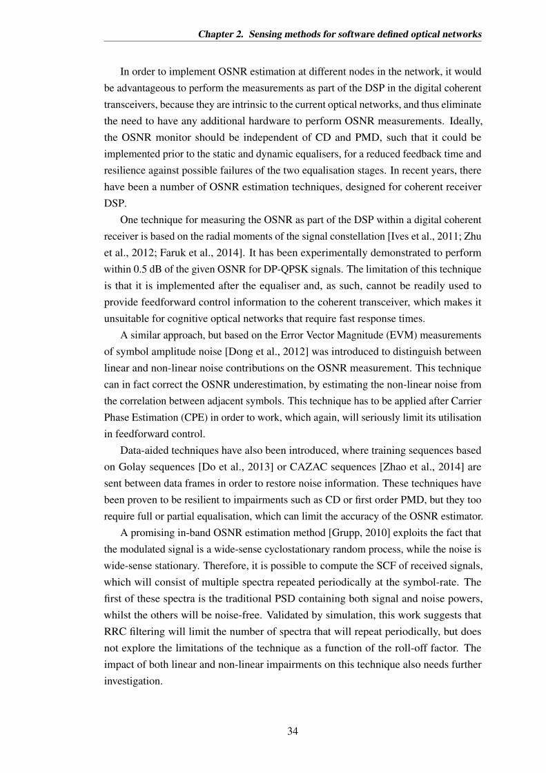
In order to implement OSNR estimation at different nodes in the network, it wouldbe advantageous to perform the measurements as part of the DSP in the digital coherenttransceivers, because they are intrinsic to the current optical networks, and thus eliminatethe need to have any additional hardware to perform OSNR measurements. Ideally,the OSNR monitor should be independent of CD and PMD, such that it could beimplemented prior to the static and dynamic equalisers, for a reduced feedback time andresilience against possible failures of the two equalisation stages. In recent years, therehave been a number of OSNR estimation techniques, designed for coherent receiverDSP.
One technique for measuring the OSNR as part of the DSP within a digital coherentreceiver is based on the radial moments of the signal constellation [Ives et al., 2011; Zhuet al., 2012; Faruk et al., 2014]. It has been experimentally demonstrated to performwithin 0.5 dB of the given OSNR for DP-QPSK signals. The limitation of this techniqueis that it is implemented after the equaliser and, as such, cannot be readily used toprovide feedforward control information to the coherent transceiver, which makes itunsuitable for cognitive optical networks that require fast response times.
A similar approach, but based on the Error Vector Magnitude (EVM) measurementsof symbol amplitude noise [Dong et al., 2012] was introduced to distinguish betweenlinear and non-linear noise contributions on the OSNR measurement. This techniquecan in fact correct the OSNR underestimation, by estimating the non-linear noise fromthe correlation between adjacent symbols. This technique has to be applied after CarrierPhase Estimation (CPE) in order to work, which again, will seriously limit its utilisationin feedforward control.
Data-aided techniques have also been introduced, where training sequences basedon Golay sequences [Do et al., 2013] or CAZAC sequences [Zhao et al., 2014] aresent between data frames in order to restore noise information. These techniques havebeen proven to be resilient to impairments such as CD or first order PMD, but they toorequire full or partial equalisation, which can limit the accuracy of the OSNR estimator.
A promising in-band OSNR estimation method [Grupp, 2010] exploits the fact thatthe modulated signal is a wide-sense cyclostationary random process, while the noise iswide-sense stationary. Therefore, it is possible to compute the SCF of received signals,which will consist of multiple spectra repeated periodically at the symbol-rate. Thefirst of these spectra is the traditional PSD containing both signal and noise powers,whilst the others will be noise-free. Validated by simulation, this work suggests thatRRC filtering will limit the number of spectra that will repeat periodically, but doesnot explore the limitations of the technique as a function of the roll-off factor. Theimpact of both linear and non-linear impairments on this technique also needs furtherinvestigation.
34

Chapter 2. Sensing methods for software defined optical networks
2.4 Chromatic dispersion estimation techniques
In a dispersive medium, such as an optical fibre, the different frequencies of a lightpulse travel at different speeds due to the wavelength dependence on the refractiveindex. CD is a linear fibre impairment which has a quadratic phase response, describedby the transfer function:
HCD( f ) = e jψ f 2, (2.6)
where ψ =−πλ2DLc , with D dispersion coefficient, λ the reference wavelength, L fibre
length and c the speed of light in vacuum. Figure 2.11 shows the ideal phase responseof a 1000 km SSMF with a dispersion coefficient of 16.78 ps/nm, where measurementswere achieved by simulation. CD spreads the pulses in time, leading to ISI, but it hasno impact on the optical power spectrum, provided coherent detection is employed.
Frequency (GHz)-5 -4 -3 -2 -1 0 1 2 3 4 5
Car
rier
phas
e (r
ad)
-30
-20
-10
0
10
20
301000 km of SSMF
IdealMeasured
Figure 2.11: Quadratic phase response of Chromatic Dispersion.
CD estimation has been a widely researched topic in the realms of blind coherentdetection and equalisation. Data-aided CD estimators [Kuschnerov et al., 2010] basedon training symbols have been investigated, however, these have the disadvantage ofincreasing the transmission overhead. Two major blind (non-data-aided) CD estimatorshave been implemented within the digital coherent receiver, either based on the static orthe dynamic equalisers output.
Static equaliser approach
In the first category, the estimator performs a best-match search on the static equaliserwhich minimises the residual dispersion based on a cost function [Kuschnerov et al.,2009; Hauske et al., 2011]. Referring back to Fig. 2.5(a), the spectrum of the received
35

Chapter 2. Sensing methods for software defined optical networks
signal Y ( f ) is computed over blocks of length NFFT and CD compensated, giving anapproximation of the original signal spectrum X( f ):
XNFFT ,n(t, f ) = H−1CD,n( f ) ·YNFFT (t, f )
Multiple CD compensation trials are considered, scanning the possible transferfunctions of the dispersive channel with arbitrary cumulative dispersion δn,n = 1,Ntrials:
HCD,n( f ) = e jψn f 2= e−πλ2·δn/c (2.7)
This technique then computes the circular autocorrelation of the spectrum at a giventime, for each assumed dispersive channel, polarisation, and a given frequency lag Ω:
RXNFFT ,n(t,Ω) =Z
XNFFT ,n(t, f )X∗NFFT ,n(t, f +Ω)d f (2.8)
Finally, the best-match cost function can be defined as the averages of Eq. 2.8 intime and across all frequency lags Ω, not equal to the symbol-rate Fb:
JMIN(n) = ∑Ω6=Fb
Z ∣∣∣RXNFFT ,n(t,Ω)∣∣∣dt. (2.9)
The minimum cost function indicates the best-match cumulative dispersion.Soriano et al. [2011] alternatively shows that the cost function defined as the time
average of the circular spectral autocorrelation at the frequency lag equal to the symbol-rate is optimum:
JMAX(n) =Z ∣∣∣RXNFFT ,n(t,Ω = Fb)
∣∣∣dt. (2.10)
Dynamic equaliser approach
The second most common approach to estimating the CD within the coherent receiverDSP is by making use of the adaptive equaliser taps to search for the minimum dis-persion error using a gradient algorithm such as Least Mean Square (LMS) or CMA[Hauske et al., 2009]. The CD contributions is isolated from the time-varying impair-ments by operating on the tap filters:
arg
H−1CD( f )
= arg
√det(W ( f ))
=−ψ f 2. (2.11)
where the Fourier Transform of the filter taps (Fig. 2.5(b)) after the convergence ofthe gradient algorithm is:
W ( f ) = F
(wxx(t) wxy(t)wyx(t) wyy(t)
). (2.12)
36

Chapter 2. Sensing methods for software defined optical networks
Optimum chromatic dispersion estimation
A comprehensive comparison between the two approaches [Soriano et al., 2011] revealsthat the adaptive filter approach performs better, with a maximum residual dispersionerror of±150 ps/nm, and a standard deviation of 30 ps/nm, up to an absolute cumulativedispersion of 900 ps/nm. Implemented with a 15-tap LMS, the adaptive CD estimatorconvergence can potentially be slow compared to the reconfiguration time of the networknodes, which is of the sub-µs order. Lowering the number of taps would be a seriouslimitation to the estimation range of this technique. This estimator requires timing-recovery and is modulation-format dependent.
By comparison, the best-match search approach, which gives a maximum residualdispersion error of ±300 ps/nm, and a standard deviation of 76 ps/nm, for a muchwider CD range, up to 32,000 ps/nm. These results were obtained from a total of 6,208captured samples, from which 6 spectra are computed with an FFT size is 210 samples.The accuracy of the estimate depends on the CD search step and knowledge of thesymbol-rate. This approach is modulation format independent and would be preferredin modulation-agnostic networks, despite the lower estimation accuracy.
To date, very little work has been done on estimating the CD of multi-carriersignals. Typically, the symbol-rate is known a priori, and the individual channelsof a WDM signal are demultiplexed prior to CD estimation. As software-definedsuperchannels will travel together on the same optical path which is not necessarilyfixed in time, a requirement for novel CD estimators that could be applied to the entireWDM superchannel arises.
2.5 Joint monitoring techniques
Joint estimation of transmission parameters and channel impairments is highly desirable,as it can reduce the estimation time from a single computational effort, together withthe implementation cost. The three most prominent categories of joint parametersmonitoring that have so far been investigated in the literature are time-domain samplingtechniques that form asynchronous amplitude histograms, frequency domain RadioFrequency (RF) power measurements and techniques based on the equaliser taps. Otherapproaches have only been briefly investigated by the research community. Table 2.2quantifies the performance of some of the main joint estimators in the literature. All ofthe listed techniques have been developed using direct detection and the majority forsingle channels. Employing direct detection looses phase and polarisation information,limiting the capability of such estimators. Also, there is a clear division betweenmonitoring of channel impairments and monitoring of transmitter parameters, with veryfew focusing on both.
37

Chapter 2. Sensing methods for software defined optical networks
Tabl
e2.
2:Su
mm
ary
ofpr
omin
entt
echn
ique
sfo
rsim
ulta
neou
sly
estim
atin
gtra
nsm
issi
onpa
ram
eter
san
dch
anne
lim
pairm
ents
.AA
H=
Asy
nchr
onou
sA
mpl
itude
His
togr
ams;
AN
N=
Art
ifici
alN
eura
lNet
wor
ks;M
FI=
Mod
ulat
ion
Form
atId
entifi
catio
n;R
F=
Rad
ioFr
eque
ncy;
BSF
=B
and-
Stop
Filte
r;PL
L=
Phas
e-L
ocke
dL
oop;
PM=
Pola
risa
tion-
Mul
tiple
xed;
*=
Roo
tMea
nSq
uare
dE
rror
valu
es.
Ref
eren
ceTe
chni
que
Para
met
ers
Ran
geA
ccur
acy
Mod
ulat
ion
Dat
a-ra
teW
DM
Dra
wba
cks
Kha
net
al.[
2014
]A
AH
&B
it-ra
te—
99.7
%R
Z-O
OK
10/2
0G
b/s
No
MFI
depe
nden
tA
NN
MFI
PM-R
Z-Q
PSK
40/1
00G
b/s
PM-N
RZ
-16Q
AM
100/
200
Gb/
s
Lie
tal.
[201
4]R
Fto
neC
D0-
246.
7ps
/nm
N/A
NR
Z-D
QPS
K80
Gb/
sN
oB
SFof
fset
fixed
DG
D0-
50ps
N/A
to10
GH
z
Yia
ndY
u[2
013]
AA
HC
D0-
425
ps/n
m20
ps/n
mN
RZ
-DPS
K10
Gb/
sN
oC
Dlim
ited
OSN
R15
-30
dB1
dBD
QPS
K20
Gb/
s(>
425
ps/n
m)
Wen
etal
.[20
11]
Freq
uenc
yB
aud-
rate
28G
Bau
dN
/AN
RZ
-DQ
PSK
112
Gb/
sN
oC
Dlim
ited
dow
n-co
nv.
CD
-40
–40
ps/n
mN
/A(>
20ps
/nm
)&
PLL
OSN
R18
-36
dB<
1dB
Bak
er-M
eflah
etal
.[20
10]
RF
tone
CD
0-47
42ps
/nm
±10
0ps
/nm
*N
RZ
-DPS
K40
Gbs
Yes
sens
itive
tofil
ter
DG
D0-
200
ps±
4ps
*de
tuni
ngO
SNR
0-25
dB±
1dB
*
Shen
etal
.[20
10]
AA
H&
CD
0-40
0ps
/nm
9.82
ps/n
m*
RZ
-DQ
PSK
40G
b/s
No
sub-
seco
ndA
NN
DG
D0-
10ps
0.92
ps*
NR
Z-1
6QA
Mpr
oces
sing
;O
SNR
10-3
0dB
0.43
dB*
com
plex
trai
ning
And
erso
net
al.[
2009
]A
AH
CD
0-70
0ps
/nm
±11
ps/n
m*
NR
Z-D
PSK
40G
b/s
No
sub-
seco
ndD
GD
0-20
ps±
0.75
ps*
RZ
-DPS
Kpr
oces
sing
Hau
ske
etal
.[20
08]
FIR
filte
rC
D-2
000-
2000
ps/n
m±
63ps
/nm
*PD
M-R
Z-D
QPS
K11
1G
b/s
No
conv
erge
nce
coef
ficie
nts
DG
D0,
30,6
0,90
ps±
4ps
*tim
elim
ited
OSN
R12
-24
dB<1
dB
38

Chapter 2. Sensing methods for software defined optical networks
2.5.1 Time domain sampling techniques
In the first category, [Anderson et al., 2009] proposed combining asynchronous delaytap sampling with statistical machine learning in order to estimate CD and DifferentialGroup Delay (DGD). This monitor consists of a direct-detector, two slow ADCs of theorder of kSa/s and a tunable delay-line. The incoming signal is sampled twice, suchthat the second set of samples are 1 bit delay apart from the first set. Plotted againsteach other, the pair of samples create a phase portrait of the waveform. Compared to aneye diagram, obtained through a singular sampling over a few bit periods to show thechange in amplitude over time, the phase portrait shows the joint Probability DensityFunction (PDF) of the amplitude and slope of the signal with respect to time. Thisenriched capture of information is exploited to estimate a wide range of transmissionimpairments. OSNR, CD, PMD, interferometric crosstalk have different imprints onthe phase portrait, and so they can simultaneously be extracted with pattern recognitionbased on statistical learning. This last stage is achieved by sweeping over a wide rangeof scenarios and “learning” the outcome of the phase portrait, but it is time-consumingprocess with up to 3 hours necessary to complete a training over 1200 scenarios. As thisconfiguration stage can be done off-line, it is not a major limitation of the technique.On the other hand, the processing speed is of the sub-second order (<0.2 s), which isnot sufficiently fast for burst-switched networks.
Demonstrated only for two level modulation formats (Return-to-Zero (RZ)- and Non-Return-to-Zero (NRZ)-Differential Phase-Shift Keying (DPSK)), the technique wouldencounter difficulties with higher order modulations, such as QPSK or 16-QAM. As thenumber of amplitude levels increases, the complexity of distinguishing them under theimpact of a combination of impairments also increases. When additionally consideringWDM signals, demultiplexing is required to apply this time-domain technique, whichwould further increase the complexity and lower the processing speed. [Khan et al.,2014] shows that the asychronous sampling method requires a resolution of about 12x12bins such that the pattern of the two-dimensional phase portrait will be maintained,which can be easily achieved with existing ADC technology.
2.5.2 Frequency domain techniques
A spectral technique based on the RF power tone [Baker-Meflah et al., 2010] has beendemonstrated by simulation and experimentally, having the capability to jointly andindependently estimate multiple impairments such as OSNR, CD and DGD. The relativephases of a selected RF tones determine the CD and PMD effects, while the amplitudeof the same tone with respect to the average signal power determine the OSNR. Thistechnique is particularly sensitive to filter detuning, such that more than 2 GHz offsetfrom the International Telecommunication Union (ITU) grid results in more than 1 dB
39

Chapter 2. Sensing methods for software defined optical networks
OSNR estimation error.
2.5.3 FIR filter coefficients techniques
The dynamic equaliser of digital coherent receivers implemented as an FIR filterprovides a means to estimate the CD, DGD and OSNR [Hauske et al., 2008, 2009] afterconvergence is achieved. This joint estimator is robust and accurate (Table 2.2), butit relies on the convergence speed of the adaptive equaliser. Even though fast blindestimators that can converge within 200 ns have been demonstrated [Thomsen et al.,2011], most algorithms require up to 25 µs to fully converge. This technique could beapplied to WDM signals, after demultiplexing and clock recovery of each channel.
2.6 Conclusions
A currently proposed solution for increasing the capacity of optical communications isby employing WDM superchannels. Whilst leveraging from legacy WDM transmissionand reception systems, WDM superchannels require more tightly spaced sub-channels,achievable through flexible grid technology and narrow Nyquist pulse-shaping. SDONcomes as a means to enable the operation of WDM superchannels, as well as enablingapplication-specific transmission characteristics. Section 2.1 of this chapter presentedthe motivation behind SDON, with specific examples of what transmission parametersare likely to be modified in software. The configuration of programmable transmittersand receivers have been discussed, with their specific constituent components. Asynthesis of the breakthrough development of flexible-grid superchannels is also given.
The second part of this chapter focused on monitoring techniques for optical net-works, a broad subject of discussion, as the necessity of ensuring effective transmissionof information over fibre has for long been acknowledged. As the conditions of theSDONs are dyanmic, existing channel impairments estimation techniques are not al-ways applicable. Firstly, not all past monitors are performed digitally, although thisis currently the most promising solution allowing the cheap integration of multipleestimators in the already existing digital coherent receivers. The reconfiguration time ofcoherent transceivers and the time required for the DSP to recover the data is of the µs
order, thus setting a similar time-limit for future monitoring techniques.This chapter introduced some of the most common symbol-rate, OSNR, CD and
joint monitoring techniques and discusses their issues regarding their applicability toSDONs. Previous approaches for estimating the symbol-rate (such as the Wavelettransform, time-domain zero crossing or nonlinearity induced spectral peaks) can beimplemented within the DSP, but they are sensitive to CD and PMD. For Nyquistor Super-Nyquist WDM superchannels it is preferred to estimate the OSNR in-band
40

Chapter 2. Sensing methods for software defined optical networks
rather than out-of-band in order to avoid the issues associated with small guard bandsand filtering effects. As coherent receivers translate the optical signal linearly into theelectrical domain, preserving its phase and polarisation information, means that CDestimators are naturally suitable to be implemented within their DSP. Such techniqueshave successfully been demonstrated based on the channel equalisers, however theyrequire demultiplexing of the individual sub-channels. Joint monitors are usually robustand more cost efficient, but these have been mainly specialised to parameters belongingto either the transmission setup or the optical channel.
Novel estimators suitable for software-defined Nyquist-WDM superchannels, tobe implemented within the coherent receiver DSP are therefore required, preferablyperformed jointly as part of a single computational effort. The next chapter constitutesthe theoretical background behind the monitoring techniques proposed in this work.
41

3Statistical and spectral properties of
digitally modulated optical signals
Spectral analysis is a powerful tool in the investigation of properties of signals, par-ticularly when these are corrupted by noise. This chapter describes statistical andspectral properties of digitally modulated optical signals, from which a few novel prac-tical spectral techniques will be derived in the subsequent chapters, for the purposeof signal characterisation and channel estimation. The PSD is traditionally employedfor measuring the OSNR, but can also be used within the digital coherent receiver toestimate the symbol-rate of the signal, as it will be demonstrated in Chapter 4. TheSCF, a generalisation of the PSD, further exploits the cyclostationarity property oflinearly modulated signals, to help distinguish their underlying periodicities, whenthese are hidden in the PSD. The time domain counterparts of the PSD and SCF arethe autocorrelation and the CAF respectively, which are also explained here. Chapter5 will explore cyclostationarity for the estimation of a number of parameters. Thepresent chapter, sets the background knowledge required for the understanding of thetechniques demonstrated in this thesis. Established practical implementations of theSCF are also presented. Both the continuous and the discrete signal representations arebeing considered.
To illustrate these concepts, a simple transmission model is assumed, as depictedin Fig. 3.1: a linearly modulated signal x(t), of symbol-period Tb, undergoes pulseshaping at the transmitter and is corrupted by noise arising from optical amplification
42

Chapter 3. Statistical and spectral properties of digitally modulated optical signals
during transmission over L km of optical fibre. The signal is subsequently detected by acoherent receiver, in which the ADCs sample at Fs rate and NADC number of samplesare captured, corresponding to ∆t observation time interval.
x(t)
n(t)
Optical
90o
hybrid
ADC
LO laser
ADC
Coherent Receiver
Fs
y(nTs)x-pol
y-polL km fibre
ChannelTransmitter
Po
l-m
ux
AWGN
RRC
RRC
LPF
LPF
Data
x-pol
Data
y-pol
Analog Digital
Δt
Tb
+1
-1
+1
-1 or NADC samples
Figure 3.1: Simple transmission model assumed for the exemplification of the conceptsin this chapter. The modulation format can be any M-PSK or M-QAM types (hereBPSK is depicted).
The Amplified Spontaneous Emission (ASE) noise is modelled as Additive WhiteGaussian Noise (AWGN) and has different statistical properties from the signal. AWGNis a wide-sense stationary process, as its mean and autocorrelation are time-invariant.Signals that have an underlying periodicity due to modulation, multiplexing and/orsampling will be wide-sense cyclostationary [Gardner et al., 2006], meaning that theirmean and autocorrelation are periodically time-variant, but stationary within their cycle.
This chapter is structured in four sections, as follows. The first section explains andexemplifies by contrast the stationarity and cyclostationarity properties. The definitionsof the autocorrelation and Cyclic Autocorrelation Functions are also given here. Theirfrequency domain counterparts, the PSD and SCF are presented in the following twosections. Finally, the impact of the Nyquist pulse shaping filter on the SCF is discussedin the last section. For reference, the definitions of these signal properties are also givenin Appendix D.
3.1 Autocorrelation function of stationary and cyclosta-tionary processes
The autocorrelation function measures how much the complex field of a signal sampledat two time instances, which are separated by a fixed delay τ are correlated to (orresemble) each other. The parameter τ is called the time lag of the autocorrelation. Twoalternative models of the autocorrelation are possible: either based on the assumptionthat the signal is a stochastic process, or that the signal is a time-series function [Gardner,1991]. This section introduces the cyclostationarity property in terms of the stochasticand non-stochastic definitions of the CAF.
43

Chapter 3. Statistical and spectral properties of digitally modulated optical signals
3.1.1 Stochastic definition
A stochastic model assumes multiple realisations of a process, such as those shown inFig. 3.2, for a binary modulated signal and AWGN, for example. Ideally, all possiblerealisations are considered. However, as this is not the case in practice, due to a limitednumber of available measurements, an estimate is obtained instead.
0 0.5 1 1.5 2 2.5 3−1
0
1
0 0.5 1 1.5 2 2.5 3−1
0
1
0 0.5 1 1.5 2 2.5 3−1
0
1
Tra
nsm
itte
d s
ign
al
0 0.5 1 1.5 2 2.5 3−1
0
1
0 0.5 1 1.5 2 2.5 3−1
0
1
Time (ns)t+τ
2t-τ
2
0 0.5 1 1.5 2 2.5 3−1
0
1
0 0.5 1 1.5 2 2.5 3−1
0
1
0 0.5 1 1.5 2 2.5 3−1
0
1
AW
GN
0 0.5 1 1.5 2 2.5 3−1
0
1
0 0.5 1 1.5 2 2.5 3−1
0
1
Time (ns)t+τ
2t-τ
2
Figure 3.2: Multiple realisations of a zero-mean binary modulated signal (top) andAWGN of zero-mean and 0.25 standard deviation (bottom). Two samples, delayed fromeach other by τ, as indicated, are to be correlated across the whole ensemble.
44

Chapter 3. Statistical and spectral properties of digitally modulated optical signals
The first and second order statistical properties (i.e. the mean and autocorrelationrespectively), are obtained through ensemble averages:
µx = E [x(t)] , (3.1)
Rx(τ) = E[x(t +
τ
2) · x∗(t− τ
2)]. (3.2)
Conventional notations are used: x to indicate the estimated value of x, x∗ for thecomplex conjugate of x, and E for the expectation operator, which gives the ensembleaverage.
The mean of a wide-sense stationary process is time-independent while the autocor-relation depends only on the time lag. In the majority of the optical communicationsliterature, modulated signals have been assumed as wide-sense stationary processes,along with noise. However, as introduced in the seminal works of Hurd [1969] andGardner [1972], linearly modulated signals have an autocorrelation function that isperiodic with time, and therefore are not stationary in the wide-sense. These are insteaddefined as wide-sense cyclostationary, as the autocorrelation retains its stationaritywithin a fixed cycle.
The two examples considered previously demonstrate these statements. The meanvalues of both the binary modulated signal and the AWGN process are clearly zero.The autocorrelations on the other hand, exhibits different properties depending on theprocess considered, as Fig. 3.3 shows. Based on a large number of different realisationsof a binary signal, Fig. 3.3(a) shows that the autocorrelation function will be cyclicin time, and the correlation is non-zero provided that the two samples which are tobe correlated fall within the same clock interval. By contrast, the autocorrelation of awide-sense stationary process as a function of both time and time lag is depicted in Fig.3.3(b). Here, there is clearly no time-dependence and there is no correlation for anyτ 6= 0, because the different samples of a random process are independent from eachother and therefore they do not correlate.
Therefore, under the cyclostationarity theory, the autocorrelation function will de-pend on two parameters: the time instant t, when the measurement is performed, and thetime lag τ. The mathematical notation of the autocorrelation of the cyclostationary signalx(t) becomes Rx(t,τ), instead of Rx(τ) as before, to underline its time-dependency.
These conclusions lead to the formal stochastic definition of cyclostationarity,whichstates that a signal is wide-sense cyclostationary (or cyclostationary of the second order)if its autocorrelation function is periodic with time:
Rx(t,τ) = Rx(t +Tb,τ). (3.3)
45

Chapter 3. Statistical and spectral properties of digitally modulated optical signals
Samples correlate
if they are within the
same clock cycle.
Time periodic
Wide-sense
cyclostationary
(a)
Each sample correlates
only with itself.
Time invariant
Wide-sense
stationarity
(b)
Figure 3.3: The autocorrelation function of binary modulated signals is cyclic in time,demonstrating that these are wide-sense cyclostationarity processes (a), while AWGNis time-invariant, as it is a wide-sense stationary process (b).
As a periodic function, the autocorrelation therefore has a Fourier series expansion,which is given by:
Rx(t,τ) =+∞
∑n=−∞
Rn
Tbx (τ) · e j2π
nTb
t, (3.4)
where:
• Rn
Tbx (τ) constitute the Fourier series coefficients of the autocorrelation function,
called the Cyclic Autocorrelation Functions,
• α = nTb
,n ∈ Z are the Fourier series frequency components, which are called thecyclic frequencies, and
• Tb is the both the symbol period and the autocorrelation period.
Fig. 3.4 shows in more detail, the inherent periodicity of the autocorrelation functionwith time, for a fixed lag value. The duration over which the autocorrelation is not
46

Chapter 3. Statistical and spectral properties of digitally modulated optical signals
identically zero, decreases as the lag parameter increases. For any lag value higherthan the symbol period Tb, the autocorrelation will be zero, as consecutive symbols areuncorrelated (they are assumed independent and identically distributed).
0 Tb 2Tb 3Tb 4Tb 5Tb 6Tb 7Tb 8Tb 9Tb 10Tb
0
0.5
1
Time (s)
Cyc
lic a
utoc
orre
latio
n
τ=0
0 Tb 2Tb 3Tb 4Tb 5Tb 6Tb 7Tb 8Tb 9Tb 10Tb
0
0.5
1
Time (s)
Cyc
lic a
utoc
orre
latio
n
τ=0.25 × Tb
0 Tb 2Tb 3Tb 4Tb 5Tb 6Tb 7Tb 8Tb 9Tb 10Tb
0
0.5
1
Time (s)
Cyc
lic a
utoc
orre
latio
n
τ=0.5 × Tb
0 Tb 2Tb 3Tb 4Tb 5Tb 6Tb 7Tb 8Tb 9Tb 10Tb
0
0.5
1
Time (s)
Cyc
lic a
utoc
orre
latio
n
τ=1.5 × Tb
Figure 3.4: The autocorrelation of a modulated signal is cyclic in time, for a fixed timelag τ. The autocorrelation period is equal to the symbol period.
3.1.2 Deterministic definition
A deterministic definition implies a time average over the entire signal, which is regardedas a single time-series measurement. This is a direct consequence of the ergodicityproperty of stationary processes, for which the ensemble average is equal to the timeaverage. Thus, the mean of x(t) is:
µx = limT→∞
1T
Z T2
− T2
x(t)dt (3.5)
and the autocorrelation is given by:
Rx(τ) = limT→∞
1T
Z T2
− T2
x(t +τ
2)x∗(t− τ
2)dt (3.6)
47

Chapter 3. Statistical and spectral properties of digitally modulated optical signals
The stochastic and deterministic (non-probabilistic) definitions are equivalent toeach other, as the ensemble averaging is replaced by time averaging [Gardner, 1994].When dealing with single time-series measurements of a signal, that cannot be modelledas realisations of a process, such as it is the case in a fibre optics transmission system asthe one described previously in Fig. 3.1, it is more appropriate to use the deterministicmodel. This assumption and the following deterministic definitions of the CAF, andlater the SCF, are used subsequently in Chapter 5 of this thesis.
In deterministic terms, the signal x(t) is defined as second-order cyclostationary ifthere exists a quadratic time-invariant transformation that, when applied to the signal, itinduces finite-strength additive sine-wave components, that were not contained in x(t)before the transformation [Gardner, 1986a]. Linearly modulated signals are second-order cyclostationary, as there is such a second order transformation, namely the lagproduct z(t) = x(t + τ
2)x∗(t− τ
2), that contains sine-wave components at frequencies α
proportional to the symbol-rate. These components are the CAFs and the frequenciesare called cyclic frequencies.
The CAF is, more simply, defined as the time average of the autocorrelation lag prod-uct weighted at a frequency component α (in other words, the sine-wave components ofthe lag product function):
Rαx (τ) = lim
T→∞
1T
Z T2
− T2
x(t +τ
2)x∗(t− τ
2)e− j2παtdt (3.7)
0 Tb/2 Tb 3Tb/20
0.2
0.4
0.6
0.8
1
Time lag (s)
Nor
mal
ised
cyc
lic a
utoc
orre
latio
n
α = 0 Hzα = 0.5⋅Fbα = 1⋅Fbα = 1.5⋅Fbα = 2⋅Fbα = 2.5⋅Fbα = 3⋅Fb
Figure 3.5: The Cyclic Autocorrelation Function is not identically zero only for cyclicfrequencies which are multiples of the symbol-rate. Here, square pulses with no low-pass filtering are assumed.
48

Chapter 3. Statistical and spectral properties of digitally modulated optical signals
Fig. 3.5 shows the CAF, as a function of the time lag τ and the cyclic frequencyα. For linearly modulated signals, the cyclic frequency α is defined over a set Ay =m ·Fb | m ∈ Z, where Fb is the symbol-rate and the inverse of the symbol period Tb.Over this set, the Cyclic Autocorrelation Functions constitute the Fourier coefficients ofthe autocorrelation, which is thus given by:
Ry(t,τ)∆= ∑
α∈Ay
Rαy (τ) · e j2παt (3.8)
−Fs 5Fb −3Fb −Fb 0 Fb 3Fb 5Fb Fs0
0.1
0.2
0.3
0.4
0.5
0.6
0.7
0.8
0.9
1
Cyclic frequency (GHz)
Nor
mal
ised
cyc
lic a
utoc
orre
latio
n
(a) QPSK signals are wide-sense cyclostationary as their auto-correlation contains frequency components at cyclic frequen-cies multiple of the symbol-rate.
−Fs 5Fb −3Fb −Fb 0 Fb 3Fb 5Fb Fs0
0.1
0.2
0.3
0.4
0.5
0.6
0.7
0.8
0.9
1
Cyclic frequency (GHz)
Nor
mal
ised
cyc
lic a
utoc
orre
latio
n
(b) AWGN is wide-sense stationary as each frequency compo-nent correlates only with themselves (α = 0)
Figure 3.6: Cyclic frequencies components of the autocorrelation function, called theCyclic Autocorrelation Functions.
The DC component of the lag-product z(t), when α = 0, is simply the ordinaryautocorrelation function (from Eq. 3.6). In general, when α = m ·Fb, for any non-zero
49

Chapter 3. Statistical and spectral properties of digitally modulated optical signals
integer m, the Rαx (τ) is the mth harmonic of the autocorrelation function. The presence
of these harmonics indicates a cyclostationary process, as Fig. 3.6(a) shows for a QPSKsignal, where the frequency components of Rx(t,τ) exist only at integer multiples of thesymbol-rate and are identically zero otherwise. Stationary processes do not have anyharmonics within their autocorrelation, as demonstrated by Fig. 3.6(b) for AWGN.
It can be easily proved that the CAF of x(t) is equivalent to the cross-correlation oftwo signals u(t) = x(t) · e−iπαt and v(t) = x(t) · eiπαt [Gardner, 1986a]:
Rαx (τ) = Ruv(τ) = lim
T→∞
1T
Z T2
− T2
u(t +τ
2)v∗(t− τ
2)dt. (3.9)
The cyclic autocorrelation should not be confused with the circular autocorrelation.The former, as presented in this section, measures the presence of harmonics in theautocorrelation function of a cyclostationary signal, (with fundamental frequency equalto the symbol-rate when linearly modulated), hence the term cyclic. The latter, asdescribed in [Oppenheim and Schafer, 2010], simply indicates the implementation ofthe autocorrelation function of a stationary signal by circularly shifting the signal intime to obtain different lags, hence the term circular.
3.2 Power spectral density
Through spectral analysis, a signal is decomposed into its constituent frequencies tomeasure the power distribution over these frequencies. This measurement represents thePSD of the signal, which can be used in a myriad of ways for signal analysis. One suchuse for example, is in the OSNR measurement using the OSA approach, as described inSection 2.3.
As an ideal PSD measurement is not possible in practice, due to the limited samplingrate and measurement time, different techniques have been devised in order to estimatethe PSD of a signal, as accurately as possible. Some of the simplest and most effectivetechniques are directly derived from the Fourier transform of the signal.
To account for the fact that the signal is observed over a finite time interval, we usehere the Short-Time Fourier Transform (STFT) in order to inspect the spectral contentof the signal. The STFT is a FFT performed at time t over a window of arbitrary intervalT , or in other words, it measures the spectral content with respect to time:
XT (t, f ) =Z t+ T
2
t− T2
x(γ)e j2π f γdγ (3.10)
Equation 3.10 holds under the assumption that the window is rectangular. Theperiodogram is the most commonly used PSD estimate, and it is obtained by applyingthe STFT over the entire measured signal. Analytically, the PSD is given by the squared
50

Chapter 3. Statistical and spectral properties of digitally modulated optical signals
magnitude of the STFT, inversely scaled by the measurement time interval, T (in thisparticular case T = ∆t):
SxT (t, f ) =1T|XT (t, f )|2 (3.11)
The periodogram is a good estimate of the PSD provided that the SNR is high andthe measurement time is sufficiently long. If this is not the case, the PSD will exhibithigh variance (low estimation reliability).
An alternative approach to PSD estimation is Welch’s method, which averagesmultiple periodograms over shorter intervals T = 1
∆ f , within the entire signal interval∆t:
Sx( f ) = lim∆ f→0
lim∆t→∞
1∆t
Z t+ ∆t2
t−∆t2
Sx1/∆ f (ξ, f )dξ (3.12)
The averaging operation will thus reduce the variance due to noise, when the SNRis low.
According to the Wiener-Khinchin relation, the PSD of a stationary random signalis obtained from the Fourier Transform of the autocorrelation1 of the signal:
Sx( f ) = F
Rx(τ)
=Z +∞
−∞
Rx(τ)e− j2π f τdτ (3.13)
3.3 Spectral correlation function
Similarly to the autocorrelation function, which measures the correlation between time-domain samples separated by a time lag, the SCF measures the density of the correlationbetween the spectral components separated by a cyclic frequency α. This correlationis measured in both amplitude and phase. Since a cyclostationary signal exhibits timeperiodicity in its autocorrelation, with period equal to the symbol-period Tb, then itsSCF exhibits periodicity with a fundamental frequency equal to the symbol-rate Fb = 1
Tb.
Parallels between the SCF and PSD are drawn here, in order to explain the basiccyclostationarity concepts in the frequency domain. A few digital SCF implementationshave been proposed in the literature and are discussed here. The SCF is sometimesreferred to as the Spectral Correlation Density Function or cyclic spectra. In the workpresented in Chapter 5, the slice of SCF at α = Fb is specifically referred to as the cyclic
spectrum and the process of obtaining it, spectral correlation.Firstly, the Wiener-Khinchin theorem (Eq. 3.13) can be extended for cyclostationary
signals, to the more general relation called the Cyclic Wiener Relation [Gardner, 1987]which states that the SCF is the Fourier Transform of the CAF:
1Using the notation for a wide-sense stationary process, as described in Section 3.1.
51

Chapter 3. Statistical and spectral properties of digitally modulated optical signals
Sαx ( f ) = F
Rα
x (τ)
=Z
∞
−∞
Rαx (τ) · e−i2π f τdτ (3.14)
The SCF is therefore defined on a bi-frequency plane, along the ordinary frequencyf and the cyclic frequency α. If the two frequency axes are normalised to the sampling-rate, then the bi-frequency plane is uniquely defined along the ranges f ∈
[−1
2 , 12
]and
α ∈ [−1,1].
−4Fb −3Fb −2Fb −Fb 0 Fb 2Fb 3Fb 4Fb0
0.2
0.4
0.6
0.8
1
Frequency (GHz)
Nor
mal
ised
spe
ctra
l cor
rela
tion
func
tion
α = 0 Hzα = 0.5⋅Fbα = 1⋅Fbα = 1.5⋅Fbα = 2⋅Fbα = 2.5⋅Fbα = 3⋅Fb
Figure 3.7: The SCF is the Fourier transform of the CAF and is not identically zeroonly for cyclic frequencies which are multiples of the symbol-rate. Here, square pulseswith no low-pass filtering are assumed.
Referring back to Fig. 3.5, the Fourier Transform of the CAF is depicted in Fig. 3.7.The ideal SCF of a purely cyclostationary signal will exhibit periodicity only for cyclicfrequencies equal to the symbol-rate and will be identically zero otherwise. The 3Drepresentation of the SCF in Fig. 3.8 helps to better visualise the difference betweenwide-sense cyclostationary and wide-sense stationary signals. The cyclic spectra isperiodic along the cyclic frequency with period equal to the symbol-rate, for signalsmodulated with a linear modulation format, such as M-PSK or M-QAM. On the otherhand, AWGN is wide-sense stationary, so its SCF is identically zero for all cyclicfrequencies, except for the special case when α = 0.
Similarly to the periodogram of stationary processes (Equation 3.11), the SCF can besimply approximated by the cyclic periodogram Sα
xT(t, f ), measured within an arbitrary
observation time T , as given by:
Sαx ( f )≈ Sα
xT(t, f ) =
1T
XT (t, f +α
2) ·X∗T (t, f − α
2). (3.15)
which also suffers from high variance at low SNRs and when the observation time is
52

Chapter 3. Statistical and spectral properties of digitally modulated optical signals
(a) QPSK signals are wide-sense cyclostationary as their SCFconsists of cyclic spectra repeating periodically at cyclic fre-quencies multiple of the symbol-rate Fb.
(b) AWGN is wide-sense stationary as only one spectrum existsat cyclic frequency α = 0.
Figure 3.8: SCF of cyclostationary (a) and stationary (b) signals.
restricted.An alternative, but equivalent, mathematical expression of the SCF is the Cross-
Power Spectral Density (CPSD) of signals u(t) = x(t) · e− j2πα
2 t and v(t) = x(t) · e j2πα
2 t ,which can be introduced in Eq. 3.9 to give:
Sαx ( f )≈ Suv(t, f ) =
1T
UT (t, f ) ·V ∗T (t, f ). (3.16)
From these two last expressions arises the interpretation of the SCF as the complexcorrelation (in both amplitude and phase) of all frequency components of x(t), separatedby an arbitrary cyclic frequency α. When α = 0, we are correlating each frequency withitself and the cyclic spectra simply reduces to the PSD, whilst the cyclic periodogram
53

Chapter 3. Statistical and spectral properties of digitally modulated optical signals
(Eq. 3.15) reduces to the conventional periodogram (Eq. 3.11). Because the correlationis performed as a complex operation, the resulting SCF is complex for all α 6= 0 and isreal otherwise.
According to Gardner [1986b], the ideal SCF of a continuous-time signal x(t) can bemore efficiently estimated either as a temporally smoothed or as a spectrally smoothedcyclic periodogram. The difference between the two smoothing approaches is given notonly by the domain onto which the averaging operation is performed, but also by thetime intervals T over which the STFT is computed (i.e. in Eq. 3.15).
Temporal smoothing
Temporal smoothing is achieved by averaging multiple STFTs obtained over fractionaltime intervals of the measured signal (T = 1
∆ f ).
Sαx ( f ) = lim
∆ f→0lim
∆t→∞
1∆t
Z t+ ∆t2
t−∆t2
Sαx1/∆ f
(ξ, f )dξ (3.17)
A graphical representation of the temporal smoothing technique is shown in Fig.3.9. The captured signal of total time duration ∆t is divided into shorter segments ofduration T = 1
∆ f . Multiple cyclic periodograms are first computed over these differenttime slots, having a spectral resolution equal to ∆ f . The individual periodograms aresubsequently averaged in time. In the cyclostationarity theory, the time-smoothing SCFis the equivalent of the Welch method for obtaining an improved PSD estimate, byreducing the impact of random effects through averaging. As a confirmation to thisstatement, when α = 0, Eq. 3.17 becomes Eq. 3.12.
The spectral estimation variance can therefore be lowered, by increasing the numberof averages. In order to do so, the total observation time must greatly exceed theduration of the time segments:
∆t >> T =1
∆ f(3.18)
Additionally, the segments could be overlapping in order to increase the number ofaverages, for a fixed ∆t. However, increasing the number of averages has the disadvan-tage of increasing the computational complexity of the technique, when implemented inthe digital domain. Several methods have been proposed for implementing the temporalsmoothing approach, with differing levels of complexity.
54

Chapter 3. Statistical and spectral properties of digitally modulated optical signals
X1/Δf(t,f)
SX(f)α
ΔfNSCF.0
Δf
Temporal-smoothing
Δt
1/Δf NSCF
points
ΔfNSCF.0
X1/Δf(0,f)
ΔfNSCF.0
Δf
X1/Δf(ΔtΔf,f)
ΔfNSCF.0
0
ΔfNSCF.
x
X1/Δf(t,f- )2α*
0
ΔfNSCF.
SX1/Δf(t,f)Δtα
ΔfNSCF.0
Δf
Temporally-smoothed cyclic periodogram
Te
mp
ora
lly-s
mo
oth
ed
cyclic
pe
rio
do
gra
m
Te
mp
ora
lly-s
mo
oth
ed
cyclic
pe
rio
do
gra
m
SX1/Δf(0,f)Δtα
ΔfNSCF.0
Δf
SX1/Δf(ΔtΔf,f)Δtα
ΔfNSCF.0
Δf
Δf X1/Δf(t,f+ )2α
Δf
Figure 3.9: Schematic of the temporal smoothing technique to calculate the cyclicspectrum.
55

Chapter 3. Statistical and spectral properties of digitally modulated optical signals
The discrete-time temporally smoothed SCF [Tom, 1995] is given by:
Sγx(k)≈
1M ·NSCF
M−1
∑m=0
XNSCF (n+mL,k +γ
2) ·X∗NSCF
(n+mL,k− γ
2) (3.19)
where:
• γ is the discrete cycle frequency, the equivalent of the continuous α.
• k is the discrete ordinary frequency, across which each spectral slice is measured.
• n is the time index.
• M is the number of individual temporal segments.
• NSCF is the number of samples within each segment, and the FFT size.
• L is the number of samples that are skipped when moving from one segment toanother, and it indicates the amount of overlap.
The downconverted Discrete Fourier Transform (DFT) of the digital signal segmentxNSCF (n), filtered with aNSCF (n) data tapering function, here assumed to be an idealrectangular window, is:
XNSCF (n+mL,k) ∆=NSCF−1
∑n=0
aNSCF (n)x(n+mL)e− j2πk(n+mL)/NSCF (3.20)
After the multiplication the term e− j2πνmL/NSCF arises from the time-shift of thesliding window that extracts each data segment and contributes to the computation ofthe SCF by ensuring the segments are in phase.
In order to double the cyclic frequency granularity, the time segments of size NSCF ,are padded with zeros such that the total time interval is twice as long: 2NSCF . To coverthe entire bi-frequency plane as shown in Fig. 3.10, 2NADCNSCF cells are computed intotal.
The brute-force approach involves the calculation of Eq. 3.19, cell-by-cell and isthe least effective. It has a complexity dominated by the temporal averaging opera-tion, which comprises of two multiplications for each cell: frequency-shifted spectramultiplications and time exponential multiplications.
56

Chapter 3. Statistical and spectral properties of digitally modulated optical signals
k
1
-1
12- 1
2
0
k0
k1=
NADC
1k=NSCF
Figure 3.10: Bifrequency plane showing the width and length of a single cell. Its totalarea can be filled with 2 ·NSCF ·NADC cells. The two frequency axes are normalised bythe sampling frequency.
Operation Number of complex multiplications2 NSCF - point FFT M NSCF (1+ log2(NSCF))
Temporal averaging for all cells 2 M NADC NSCF
Table 3.1: Implementation complexity of the brute-force time smoothed SCF.
Two well established digital implementations of the time-smoothing method, withimproved computational performance, are the FFT Accumulation Method (FAM) andthe Strip Spectrum Correlation Algorithm (SSCA). Both algorithms use an extra FFTstage instead of averaging in order to improve the resolution along the cyclic frequencyaxis. Whilst detailed investigation of these approaches does not constitute the scope ofthis thesis, they are treated in [Roberts et al., 1991] and [Brown and Loomis, 1993] .
Frequency smoothing
The STFT computed over the entire measured signal (T = ∆t):
Sαx ( f ) = lim
∆ f→0lim
∆t→∞
1∆ f
Z f + ∆ f2
f−∆ f2
Sαx∆t
(t,ν)dν (3.21)
A graphical representation of the spectral smoothing approach, for the computationof the SCF, is shown in Fig. 3.11. Spectral smoothing is performed on a singleperiodogram, obtained from the entire measured signal (T = ∆t, where ∆t is the totalobservation time interval of x(t)). The averaging operation for reducing random effectsis performed in the frequency domain, over fixed frequency bins, such that the finalresolution of the cyclic spectrum is ∆ f .
To better reduce the effects of randomness causing a high estimation variance, thenumber of averages is increased, which in this case it is equivalent to the bandwidth of
57

Chapter 3. Statistical and spectral properties of digitally modulated optical signals
Frequency-smoothed cyclic periodogram
Δt
XΔt(t,f)
0
x
XΔt(t,f+ )
00
. .1/Δt2α
XΔt(t,f- )2α*
ΔtNADC
1/Δt
Δf
0
SX(f)α
ΔfNSCF.
Spectral-smoothing
SXΔt(t,f)Δf
0
Δf
α
1/Δt
Figure 3.11: Schematic of the spectral smoothing technique to calculate the SCFSchematic of the spectral smoothing technique to calculate the cyclic spectrum.
averaging bins greatly exceed the frequency resolution of the periodogram:
∆ f >>1T
=1∆t
(3.22)
In the case of the digitized signal, ∆t = NADCFs
, while ∆ f = Fsw , where w is the number
of samples used for frequency averaging in Eq. (3.21). The frequency-smoothed SCFis thus defined over NSCF = NADC
w points. The condition 3.22 means that the frequencysmoothing window w should be significantly less than the total sample size NADC, foran increase in number of averages and, thus, a decreased variance.
58

Chapter 3. Statistical and spectral properties of digitally modulated optical signals
The discrete-time spectrally smoothed SCF [Tom, 1995] is given by:
Sγx(k)≈
1w ·NADC
w−12
∑l=−w−1
2
XNADC(n,k +γ
2+ l) ·X∗NADC
(n,k− γ
2+ l) (3.23)
where
XNADC(n,k) ∆=NADC−1
∑m=0
aNADC(m)x(n+m)e− j2πk(n+m)/NADC
is the downconverted DFT of the digital signal x(n), and:
• γ is the discrete cycle frequency, the equivalent of the continuous α.
• k is the discrete ordinary frequency, across which each spectral slice is measured.
• n is the time index.
• NADC is the total number of samples captured by the ADC and the FFT size.
• aNADC(n) is a data tapering function, here assumed to be an ideal rectangularwindow.
2NADC
FFT*
X(n,k- /2+l)
X(n,k+ /2+l)
Box
averaging Sx(k)
NSCF
xNADC(n)
Figure 3.12: Brute-force method to digitally implement the calculation of the SCF, witha single FFT and a box averaging to perform frequency smoothing.
Digitally, the brute-force method for the estimation of the SCF by frequency smooth-ing can be implemented with a single FFT and a box-average filter along the frequencyk as depicted in Fig. 3.12 and demonstrated by Brown and Loomis [1993]. In orderto double the cyclic frequency granularity, the signals, are padded with zeros suchthat the total sample size is twice the initial sample size: 2NADC. To cover the entirebi-frequency plane, 2NADCNSCF cells are computed in total. The brute-force methodimplements Eq. 3.23 cell-by-cell, and has a complexity dominated by the FFT operation(Table 3.2).
59

Chapter 3. Statistical and spectral properties of digitally modulated optical signals
Operation Number of complex multiplications2 NADC - point FFT NADC(1+ log2(NADC))
Frequency averaging for all cells 2 w NADC NSCF
Table 3.2: Implementation complexity of the brute-force frequency smoothed SCF.
Reliability and resolution trade-off
A spectrum estimate is reliable, or it has a low variance, if the random amplitude andphase components corrupting it are reduced insofar as the measurement becomes time-independent. As discussed previously for the two averaging approaches, this can beachieved by increasing the number of averages performed, as Equations 3.18 and 3.22described previously. These conditions are united under the Grenander’s Uncertainty
Condition [Gardner, 1986b], which states that for a reliable spectral estimation, theproduct between the temporal and spectral resolutions should be much greater thanunity:
∆t∆ f >> 1 (3.24)
or, for digital signal representations, the number of samples used in the estimateshould be much greater than the number of samples used to represent the final spectrum:
NADC
NSCF>> 1. (3.25)
By contrast, if the SCF would simply be approximated by the cyclic periodogram(Eq. 3.15), then ∆t ·∆ f = 1. However, when smoothing is performed, increasing thenumber of averages is equivalent to a reduced temporal resolution ∆t >> 1/∆ f whentemporal smoothing is employed, and a reduced spectral resolution ∆ f >> 1/∆t whenspectral smoothing is employed. It is not possible therefore, to maintain a high temporalor spectral resolution, as the reliability of the spectrum estimate increases.
The Grenander’s condition can also be expressed in terms of the cycle resolution
∆α = 1∆t , which indicates how finely the cyclic frequencies could be distinguished:
∆ f∆α
>> 1 (3.26)
Because the cycle resolution is the inverse of the temporal resolution and fromGrenander’s condition, the granularity of the cyclic frequency is much finer comparedto the granularity of the ordinary frequency, in the bi-frequency plane (Fig. 3.10).
In an ideal measurement, ∆ f → 0 and ∆α→ 0, meaning that the capability todistinguish ordinary and cyclic frequencies is infinite. As the number of samples andthe sampling frequency are finite in practice, spectral leakage and cycle leakage are
60

Chapter 3. Statistical and spectral properties of digitally modulated optical signals
limiting effects of the spectral measurement. A more detailed account of all of theseconcepts can be found in [Gardner, 1986b].
Temporal and spectral smoothing approaches comparison
The two smoothing approaches are equivalent to each other, as Gardner [1986b] proves,provided that the observation interval is sufficiently large (∆t >> 1/∆ f ), such thatthe impact of random effects on the estimate is diminished and the cycle resolution isincreased (∆α = 1/∆t). The temporal-smoothing approach is more computationallyefficient if the entire SCF is required, for a multitude of ordinary and cyclic frequencies,whereas, frequency smoothing is more computationally effective if the number of cyclicfrequencies of interest is limited [Roberts et al., 1991]. The work presented in this thesisfocuses on the frequency smoothing approach, because the computation of the SCF forspecific cyclic frequencies is needed.
3.4 Nyquist pulse shaping
When propagating through fibre, optical pulses experience spreading under cumulativedispersion. As the distance travelled increases, the adjacent pulses will start interfering,effect called ISI. A low-pass filter that satisfies the Nyquist ISI criterion can be employedto mitigate this distortion.
Nyquist pulse shaping additionally increases the spectral efficiency of the transmis-sion by limiting the signal’s bandwidth, whilst maintaining the same symbol-rate. Themost commonly employed Nyquist pulse shaping filter is the RC filter, split betweenthe transmitter and receiver into two RRC filters as shown in Fig. 3.13, for improvednoise suppression.
HRRC,Tx(f) Hchannel(f) HRRC,Rx(f)
Figure 3.13: Two RRC matching filters are split between the transmitter and receiver, togive an overall RC filter response.
The overall RC filter frequency response is:
HRC( f ) =√
HRRC,T x( f ) ·√
HRRC,Rx( f )
whereas, the frequency response of the RRC filter is given by:
61

Chapter 3. Statistical and spectral properties of digitally modulated optical signals
HRRC( f ) =√
HRC( f ) =
√
Tb, | f | ≤ 1−r2Tb√
Tb2
[1+ cos
(πTb
r
[| f |− 1−r
2Tb
])], 1−r
2Tb< | f | ≤ 1+r
2Tb
0, otherwise(3.27)
Fig.3.14(a) shows that the filter bandwidth is proportional to the roll-off factor, as isthe spectrum of the filtered signal. Given a roll-off factor r and a symbol-rate Fb thesignal bandwidth after RRC filtering is:
BWRRC = Fb · (1+ r). (3.28)
roll−off=0
roll−off=0.5
roll−off=1
0-FbFb2
0
- Fb2
Fb
Tb
Tb
2
(a) Frequency-domain
0
A
roll−off=0
roll−off=0.5
roll−off=1
0 Tb 2Tb 3Tb 4Tb 5Tb-Tb-2Tb-3Tb-4Tb-5Tb
(b) Time-domain
Figure 3.14: Ideal frequency response (left) and impulse response (right) of the RRCfilter for different roll-off factors.
The impulse response of the RRC filter is a sinc function, which ideally has aninfinite time-domain representation, and as a result, an infinite attenuation stop-band.However, in a realistic implementation the filter is of finite length, resulting in a finiteattenuation stop-band, particularly at lower roll-offs, as shown in Fig. 3.14(b). Sincea lower attenuation stop-band translates into higher penalties due to ICI and spectralleakage, whilst a lower roll-off factor is desirable to achieve both a better ISI suppressionand a higher spectral efficiency, a trade-off between spectral efficiency and performancethus needs to be attained.
As the RRC roll-off decreases the spectral correlation power and bandwidth decreaseas well. Fig. 3.15 depicts the dependence of the bandwidth of the first cyclic spectrumSα=Fb
x ( f ) on the roll-off factor and symbol-rate. For simplicity, assume that the cyclicspectrum is computed as the CPSD of two frequency shifted spectra (Eq. 3.16), obtainedfrom the original signal spectrum X( f ).
62

Chapter 3. Statistical and spectral properties of digitally modulated optical signals
Fb·(1+r)
Fb·r
X(f )2Fb
+
Fb·(1+r)
X(f)
f f
Fb·r
f
Spectral
multiplication
Cyclic
periodogram
X (f- )Fb
2*
S (t,f) Fb
xT
Figure 3.15: Bandwidth of the SCF at cyclic frequency equal to the symbol-rate (Fb) isthe intersection of the two frequency-shifted FFTs. The triangles are abstractions of thesignal spectrum with RRC filtering, which changes the spectral shape with roll-off.
Since the frequency separation between the two spectra is Fb, the bandwidth ofSα=Fb
x ( f ) can be deduced to be:
BW α=FbRRC =
BWRRC
2−(
Fb−BWRRC
2
)= Fb · r. (3.29)
Eq. 3.28 and 3.29 can be translated into the graph of Fig. 3.16, which, by normalisa-tion to the symbol-rate, shows the dependence of the bandwidth on the roll-off only. Aroll-off of 0 maximises the spectral efficiency, but simultaneously nullifies the measureof spectral correlation. Conversely, when the roll-off is 1, the bandwidth of the cyclicspectrum is maximised, to the detriment of the spectral efficiency, which is reduced.Whilst these results are obtained under ideal assumptions, the impact of finite filter tapson the spectral correlation is treated in Chapter 5, Section 5.1.
0 0.1 0.2 0.3 0.4 0.5 0.6 0.7 0.8 0.9 10
0.10.20.30.40.50.60.70.80.9
11.11.21.31.41.51.61.71.81.9
2
RRC roll−off factor
Cha
nnel
ban
dwid
th n
orm
alis
ed to
the
sym
bol−
rate
α = 0 Hzα = F
b
Figure 3.16: Bandwidth of the SCF as a function of RRC roll-off.
63

Chapter 3. Statistical and spectral properties of digitally modulated optical signals
Fig. 3.17 shows that as the Nyquist bandwidth ([−Fb
2 , Fb2
]) is approached, the power
in the cyclic harmonics at α = Fb,2 ·Fb,etc. is dissipated along the time lag, until theyare completely filtered out, whilst the spectral efficiency is increased.
−Fs −Fb Fb Fs0
0.5
1
Cyclic frequency (GHz)
Nor
mal
ised
CA
F
−Tb 0 Tb0
0.5
1
Time lag (s)
Nor
mal
ised
CA
F
α = 0 Hz
α = 0.5⋅Fb
α = 1⋅Fb
α = 1.5⋅Fb
α = 2⋅Fb
α = 2.5⋅Fb
α = 3⋅Fb
(a) NRZ signal
−Fs −FbFb Fs−150
−130
−110
−90
−70
−50
Frequency (GHz)
PS
D (
dBm
/Hz)
−Fs −Fb Fb Fs0
0.5
1
Cyclic frequency (GHz)
Nor
mal
ised
CA
F
−Tb 0 Tb0
0.5
1
Time lag (s)
Nor
mal
ised
CA
F
α = 0 Hz
α = 0.5⋅Fb
α = 1⋅Fb
α = 1.5⋅Fb
α = 2⋅Fb
α = 2.5⋅Fb
α = 3⋅Fb
(b) roll-off = 1
−Fs −FbFb Fs−150
−130
−110
−90
−70
−50
Frequency (GHz)
PS
D (
dBm
/Hz)
−Fs −Fb Fb Fs0
0.5
1
Cyclic frequency (GHz)
Nor
mal
ised
CA
F
−Tb 0 Tb0
0.5
1
Time lag (s)
Nor
mal
ised
CA
F
α = 0 Hz
α = 0.5⋅Fb
α = 1⋅Fb
α = 1.5⋅Fb
α = 2⋅Fb
α = 2.5⋅Fb
α = 3⋅Fb
(c) roll-off = 0.5
−Fs −FbFb Fs−150
−130
−110
−90
−70
−50
Frequency (GHz)
PS
D (
dBm
/Hz)
−Fs −Fb Fb Fs0
0.5
1
Cyclic frequency (GHz)
Nor
mal
ised
CA
F
−Tb 0 Tb0
0.5
1
Time lag (s)
Nor
mal
ised
CA
F
α = 0 Hz
α = 0.5⋅Fb
α = 1⋅Fb
α = 1.5⋅Fb
α = 2⋅Fb
α = 2.5⋅Fb
α = 3⋅Fb
(d) roll-off = 0.1
−Fs −FbFb Fs−150
−130
−110
−90
−70
−50
Frequency (GHz)
PS
D (
dBm
/Hz)
−Fs −Fb Fb Fs0
0.5
1
Cyclic frequency (GHz)
Nor
mal
ised
CA
F
−Tb 0 Tb0
0.5
1
Time lag (s)
Nor
mal
ised
CA
F
α = 0 Hz
α = 0.5⋅Fb
α = 1⋅Fb
α = 1.5⋅Fb
α = 2⋅Fb
α = 2.5⋅Fb
α = 3⋅Fb
(e) roll-off = 0.01
−Fs −FbFb Fs−150
−130
−110
−90
−70
−50
Frequency (GHz)
PS
D (
dBm
/Hz)
Figure 3.17: CAF and PSD of NRZ signals with and without RRC filtering.
64

Chapter 3. Statistical and spectral properties of digitally modulated optical signals
3.5 Summary
The computation of the PSD has so far been the established approach to characterisedigitally modulated optical signals, in terms of their constituent frequencies. However,signal periodicities occurring due to modulation, filtering or coding are not evidentfrom a conventional PSD analysis. Underlined in this chapter is a more appropriatemodel for such signals based on cyclostationarity, which takes into account these hiddenperiodicities.
Novel functions are defined in the realm of cyclostationarity theory. The SCF, whichis a generalisation of the PSD, measures the correlation density between the constituentfrequency components of the signal, separated by an arbitrary frequency difference(called cyclic frequency). Its time-domain counterpart is the CAF, as stated by theCyclic Wiener Relation. Linearly modulated signals are cyclostationary in the wide-sense, as their cyclic autocorrelation and SCF are periodic with the symbol-rate alongthe cyclic frequency. AWGN, on the other hand, is stationary as it does not exhibit sucha periodicity, its power being negligible for any non-zero cyclic frequencies. Stationaryand cyclostationary processes can therefore be easily differentiated by means of theirCAF or SCF.
A comparative table of the statistical and time-series interpretations of the cyclo-stationarity properties presented in this chapter are synthesised from [Gardner, 1986b]and [Gardner et al., 2006] in Table 3.3. The two definitions are equivalent, but from apractical perspective, the time-series approach is more appropriate.
Estimation methods of the conventional and cyclic spectra have also been presentedin this chapter. The most basic approach is the periodogram, which suffers from lowreliability. Improvements to the periodogram estimate can be made through eithertemporal or spectral smoothing techniques, and ensuring that a sufficient number ofaverages are performed to reduce the spectral variance due to random effects. In bothconventional spectral analysis and spectral analysis of cyclostationary signals, there is atrade-off between the estimation reliability and temporal and spectral resolutions.
The correlation between spectral components is reduced when filtering is present. IfRRC filtering is employed and the roll-off factor is the minimum of zero, the correlationcharacteristics of the modulated signal mimic those of stationary signals, as the spectralcorrelation periodicity is lost. As a result, consideration of the minimum roll-off must bemade when designing cyclostationarity-based monitoring techniques, as high spectralcorrelation and high spectral efficiency are mutually exclusive.
The following chapters demonstrate novel performance monitoring techniques, thatmake use of the spectral and statistical properties of modulated signals and noise,and that can be implemented as part of the DSP stage of coherent transceivers. Thelimitation due to the RRC filtering on these techniques is investigated.
65

Chapter 3. Statistical and spectral properties of digitally modulated optical signals
STOCHASTIC PROCESSES TIME-SERIESAutocorrelation function
Rx(t,τ)∆= E
x(t + τ
2) · x∗(t− τ
2)
Rx(t,τ)∆= 1
∆t
∆t/2R−∆t/2
x(t + τ
2) · x∗(t− τ
2)dt
Second-order cyclostationarity in the wide-sensex(t) is a cyclostationary process if its
mean and autocorrelation are periodic:x(t) is a cyclostationary signal if its lag
product z(t,τ) = x(t + τ
2) · x∗(t− τ
2)contains finite-strength sine-wave
components at α ∈ A, the countable set:E x(t +Tb)= E x(t)Rx(t +Tb,τ) = Rx(t,τ) A =
kTb
k∈Z
Cyclic autocorrelation functionSince periodic, the autocorrelation has a
Fourier series decomposition:The autocorrelation function is the
summation of its sine-wave components:
Rx(t,τ) =∞
∑n=−∞
Rn
Tbx (τ)e j2π
nTb
t Rx(t,τ) = ∑α∈A
Rαx (τ)e j2παt
where the Fourier coefficients Rn
Tbx (τ) are
the Cyclic Autocorrelation Functionswhere Rα
x (τ) are the non-stochasticCyclic Autocorrelation Functions
Rn
Tbx (τ) ∆=
1Tb
−Tb/2ZTb/2
Rx(t,τ) · e− j2π
nTb
tdt Rαx (τ) ∆= lim
∆t→∞
1∆t
∆t/2Z−∆t/2
z(t,τ) · e− j2παtdt
Spectral Correlation Density Function (or cyclic spectrum)The cyclic spectrum at cyclic frequency α is defined as the Fourier Transform of
the cyclic autocorrelation function, property known as the Cyclic Wiener Relation:
Sαx ( f ) ∆=
∞R−∞
Rαx (τ)e− j2π f τdτ
or, the cross-spectral density of spectra frequency shifted by α from each other,giving the Cyclic Periodogram (the product inside the average) which can be eithertime-smoothed (T = 1
∆ f ) or frequency-smoothed (T = ∆t), for increased reliability:
Sαx ( f ) ∆= lim∆ f→0 lim∆t→∞
⟨ 1T XT (t, f + α
2 )X∗T (t, f − α
2 )⟩
where XT (t, f ) =R T/2−T/2 x(u) · e− j2π f udu, is the Short-time Fourier Transform.
Table 3.3: Summary of cyclostationarity properties and definitions.
66

4Symbol-rate estimation based on the
power spectral density
The method presented in this chapter uses the signal power spectrum to estimate thesymbol-rate and is, as a result, CD and 1st order PMD tolerant. It is also independent ofthe IF, as long as the signal spectrum does not fall outside of the receiver bandwidth.Having the advantage of being independent on CD, PMD and LO frequency offset,this method can be employed at the beginning of the DSP stage of the digital coherentreceiver, as shown in Fig. 4.1. The main purpose of this estimator is to provide feedbackinformation to the control plane, for spectral resource optimisation as discussed inChapter 1. It can also be used as a control input to the timing recovery stage, forexample.
The estimator is applicable to both M-PSK and M-QAM signals since their powerspectral densities are identical [Couch, 1993, p.391]. Two methods are presented.Firstly, a MMSE approach with continuous ideal test spectra is proposed, but it is shownto be highly dependent on the moving-average filter applied. The second method isbased on measuring the standard deviation of the spectrum, and is shown to operatefrom 4 to 25 GBaud QPSK signals with a maximum estimation error of 2% at the FEClimit of 3.8 ·10−3, when a RRC filter with a roll-off of 0 is used.
67

Chapter 4. Symbol-rate estimation based on the power spectral density
Optical
90o
hybrid
ADC
LO laser Baud estimation
Tim
ing r
eco
ve
ry
Eq
ualis
atio
n
Carr
ier
reco
ve
ry
Slic
er
an
d d
eco
de
r
Err
or
co
un
ter
ADC
Coherent ReceiverDigital Signal Processing
50 GSa/s16 GHz
Signal
Control plane
Figure 4.1: Digital coherent receiver including a symbol-rate estimation stage for QPSKsignals.
4.1 MMSE with continuous ideal test spectra
4.1.1 Simulation setup
The symbol-rate estimation method depicted in Figure 4.2 is based on a MMSE ap-proach. The method is based on spectral matching between the transmitted signal ofunknown symbol-rate and an ideal signal of known symbol-rate. At the transmitter, atrapezoidal waveform is generated with a given symbol-rate to be estimated. AWGN isloaded onto the signal, before it is resampled at the receiver, at 50 GSa/s sampling rate.
MMSE
Bessel filter
50% of
baud-rate
RRC
(β = 0)Butterworth
16 GHz
|FFT|2
Tx Rx DSP
ADC
FADC = 50 GHz
NRZ
Data
AWGN
Baud
rate
Channel
Pulse
shaping
Power
spectrum
Analytical
spectrum
1-25 GBaud
PRBS 2 - 17Moving
average
Figure 4.2: Simulation setup for MMSE with a large number of analytical test values.
The spectrum of the transmitted signal is then smoothed by a moving average filter.The length of the moving average filter (NMA) is fixed based on the total number ofsamples captured (NADC):
NMA =NADC
25 (4.1)
A range of ideal spectra is generated, assuming ideal trapezoidal waveforms ofsymbol-rates between 0.2 and 40 GHz, that are the test values of the symbol-rates to beestimated. The ideal spectra of the analytical model correspond to a trapezoidal signal,with the same frequency grid as the transmitted signal. The spectra of a trapezoidalwaveform is given by [Paul, 2006, p.118]:
68

Chapter 4. Symbol-rate estimation based on the power spectral density
X( f ) =2A
τr(2π f )2
[cos(
2π fτ
2
)− cos
(2π f
(τ
2+ τr
))], (4.2)
where:A = maximum signal level,τ = symbol length - sampling length,τr = sampling length,f = frequency grid.
The MMSE block estimates the symbol-rate by taking the minimum error corre-sponding to the difference between the spectra of the received signal and the generatedideal test spectra. The best value is determined through an unconstrained nonlinearoptimisation.
The MSE is defined as:
mse(test) = |Etest(ω)|2−|Emeasured(ω)|2 (4.3)
The MMSE is the minimum MSE value between all the test cases, which leads tothe estimation of the symbol-rate:
Fb = argtest minmse(test). (4.4)
4.1.2 Performance analysis
The method’s performance was evaluated as the signed estimation error with respectto different noise loading conditions (Fig. 4.3(a)) and number of captured samples(Fig. 4.3(b)). The method is independent of the SNR level, but depends on increasingthe number of ADC captured samples in order to reduce the estimation error. Whilethe estimator performs well for higher symbol-rates (<5% error), it results in highoverestimation at low symbol-rates (approximately 20% error) due to the fact that themoving-average filter is not correctly optimised in those cases. More precisely, themoving-average length is too long at low symbol-rates, leading to a spreading of thespectrum, hence the overestimation. The dependence of the moving-average filter onthe symbol-rate leaves this method inefficient for blind symbol-rate estimation.
69

Chapter 4. Symbol-rate estimation based on the power spectral density
0 5 10 15 20 25 30 35−5
0
5
10
15
20
25
SNR (dB)
Signed error (%)
4096 processed samples
2.5 GBaud
10 GBaud
25 GBaud
(a)
10 11 12 13 14 15−5
0
5
10
15
20
25
30
log2(Captured samples at the ADC)
Signed error (%)
SNR = 10 dB
2.5 GBaud
10 GBaud
25 GBaud
(b)
Figure 4.3: Signed estimation error of the MMSE approach verified by simulation ofNRZ signals. (a) Impact of noise and (b) impact of captured samples.
4.2 Symbol-rate estimation based on the spectral stan-dard deviation
4.2.1 Technique description
The metric of the proposed symbol-rate estimation technique uses the standard deviationof the received power spectrum. Regarding the spectrum as a probability densityfunction, the spectral standard deviation can be defined as the second order non-centralmoment:
σ =R
( f −µ)2S( f )d fRS( f )d f
(4.5)
70
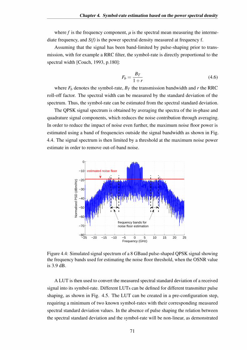
Chapter 4. Symbol-rate estimation based on the power spectral density
where f is the frequency component, µ is the spectral mean measuring the interme-diate frequency, and S(f) is the power spectral density measured at frequency f.
Assuming that the signal has been band-limited by pulse-shaping prior to trans-mission, with for example a RRC filter, the symbol-rate is directly proportional to thespectral width [Couch, 1993, p.180]:
Fb =BT
1+ r(4.6)
where Fb denotes the symbol-rate, BT the transmission bandwidth and r the RRCroll-off factor. The spectral width can be measured by the standard deviation of thespectrum. Thus, the symbol-rate can be estimated from the spectral standard deviation.
The QPSK signal spectrum is obtained by averaging the spectra of the in-phase andquadrature signal components, which reduces the noise contribution through averaging.In order to reduce the impact of noise even further, the maximum noise floor power isestimated using a band of frequencies outside the signal bandwidth as shown in Fig.4.4. The signal spectrum is then limited by a threshold at the maximum noise powerestimate in order to remove out-of-band noise.
−25 −20 −15 −10 −5 0 5 10 15 20 25−80
−70
−60
−50
−40
−30
−20
−10
0
Frequency (GHz)
Nor
mal
ised
PS
D (
dBm
/Hz)
estimated noise floor
frequency bands fornoise floor estimation
Figure 4.4: Simulated signal spectrum of a 8 GBaud pulse-shaped QPSK signal showingthe frequency bands used for estimating the noise floor threshold, when the OSNR valueis 3.9 dB.
A LUT is then used to convert the measured spectral standard deviation of a receivedsignal into its symbol-rate. Different LUTs can be defined for different transmitter pulseshaping, as shown in Fig. 4.5. The LUT can be created in a pre-configuration step,requiring a minimum of two known symbol-rates with their corresponding measuredspectral standard deviation values. In the absence of pulse shaping the relation betweenthe spectral standard deviation and the symbol-rate will be non-linear, as demonstrated
71

Chapter 4. Symbol-rate estimation based on the power spectral density
in Fig. 4.5, because of the variation in the side-lobes of the spectrum at differentsymbol-rates, within a fixed receiver bandwidth.
5 10 15 20 250
1
2
3
4
5
6
7
8
Symbol−rate (GBaud)
Spe
ctra
l sta
ndar
d de
viat
ion
(GH
z)
RRC (roll−off=1)RRC (roll−off=0.5)RRC (roll−off=0 no RRC
Figure 4.5: Look-up Table for different simulated pulse shaping cases.
The linearity between the spectral standard deviation and the symbol-rate is ensurednot only by using Nyquist pulse shaping (Fig. 4.5), but also by applying a noisethreshold (Fig. 4.6).
As expected, without noise thresholding, the noise-induced nonlinearity is higherfor lower values of OSNR, as shown in Fig. 4.6(a). Additionally, at lower symbol-rates, there are a lot more noise components in the receiver bandwidth, contributingto the standard deviation value, since the receiver bandwidth is fixed to 25 GHz toallow the measurement of signals at symbol-rates up to 25 GBaud. Therefore, theestimation of lower symbol-rates is strongly limited by noise. Here lies the motivationfor using a noise threshold. Fig. 4.6(b) shows a great improvement in the LUT when anoise threshold is applied. It is important to note here that, noise thresholding will beproblematic in Nyquist WDM systems, where the channels can be contiguous.
4.2.2 Simulation setup
The method was tested by simulation under different noise loading conditions, asshown in Fig. 4.7. QPSK signals were generated from 27−1 Pseudo-Random BinarySequences (PRBSs), to simulate typical optical signals with line-coding. The interme-diate frequency was set to be 500 kHz and the LO linewidth 100 kHz. Without lossof generality, the transmitter signal shape was trapezoidal with rise- and fall- times of10% of the symbol-rate and a RRC filter with roll-off factor of 0. The two additional
72

Chapter 4. Symbol-rate estimation based on the power spectral density
0 5 10 15 20 250
1
2
3
4
5
6
Symbol−rate (GBaud)
Spectral standard deviation (GHz)
5 dB OSNR (Monte Carlo)
10 dB OSNR (Monte Carlo)
15 dB OSNR (Monte Carlo)
20 dB OSNR (Monte Carlo)
25 dB OSNR (Monte Carlo)
30 dB OSNR (Monte Carlo)
No noise (Analyical)
(a)
0 5 10 15 20 250
1
2
3
4
5
6
Symbol−rate (GBaud)
Spectral standard deviation (GHz)
5 dB OSNR (Monte Carlo)
10 dB OSNR (Monte Carlo)
15 dB OSNR (Monte Carlo)
20 dB OSNR (Monte Carlo)
25 dB OSNR (Monte Carlo)
30 dB OSNR (Monte Carlo)
No noise (Analyical)
(b)
Figure 4.6: Impact of noise on the LUT verified by simulation of QPSK signals with215 captured samples, (a) without noise thresholding and (b) with noise thresholding.
LUT
Bessel50% of baud rate
RRC(β = 0)
Butterworth16 GHz
|FFT|2 σ
Tx Rx DSP
ADC
FADC = 50 GHz
QPSKData
1 – 25 GBaudPRBS 27 - 1
AWGN
Baudrate
Pulseshaping
Powerspectrum
Standarddeviation
Channel
Figure 4.7: Simulation setup for testing the symbol-rate estimation technique for QPSKsignals.
low-pass filters were used to account for the transmitter bandwidth limitations (5th orderBessel filter with a cut-off frequency equal to 50% of the symbol-rate) and the receiverbandwidth (16 GHz 9th order Butterworth filter, as shown in Fig. 4.8). The receiversampling frequency was set to 50 GSa/s, allowing for symbol-rates up to 25 GBaud tobe tested.
73

Chapter 4. Symbol-rate estimation based on the power spectral density
2 4 6 8 10 12 14 16 18 20−45
−40
−35
−30
−25
−20
−15
Frequency (GHz)
Am
plitu
de (
dB)
Channel 3Channel 4Bessel (5th)Butterworth (9th)Chebyshev (5th)
Figure 4.8: Tektronix Oscilloscope measured frequency characteristics. The filter givingthe closest approximation is a 9th order Butterworth filter.
4.2.3 Experimental setup
The technique was also tested experimentally for symbol-rates up to 14 GBaud. As inthe simulations, the QPSK signals were generated with a PRBS length of 27−1 andhad a trapezoidal shape with rise- and fall-times of 10% of the symbol-rate and with0 roll-off RRC. The in-phase and quadrature components of the signals are generatedwith a DAC-based Arbitrary Waveform Generator (AWG), as seen in Fig. 4.9, depictingthe experimental setup. After modulation in the optical domain, the QPSK signalswere noise loaded and subsequently converted back into the electrical domain using acoherent optical receiver with a sampling rate of 50 GSa/s. The symbol-rate estimationwas subsequently carried out using offline processing 1.
FPGA
DAC1
FPGA
DAC2
CLK
distributor
CLK
distributor
8-14GHz
8-14GHz
ECL
τ
MZI
MZI
π/2
Att
AttEDFAASE
EDFA
Coherent
Receiver
Figure 4.9: Optical back-to-back experimental setup for testing QPSK signals.
1The author is grateful to Sezer Erkılınç and Dr. Milen Paskov for their assistance with this experiment.
74

Chapter 4. Symbol-rate estimation based on the power spectral density
4.2.4 Performance analysis
Estimation accuracy
The estimation accuracy was measured by the signed percentage error:
ε =Fb−Fb
Fb·100%. (4.7)
The mean and variance of the percentage signed errors were obtained from 100different runs per symbol-rate. As shown in Fig. 4.10, the estimation accuracy increaseswith the number of captured samples. This is expected, since an increase in number ofcaptured samples is equivalent to a higher frequency granularity, resulting in a moreaccurate spectral representation of the signal. Also, as more frequency componentsenter the computation of the spectral standard deviation, the lower the variance ofthe estimation accuracy becomes. Experimentally, a minimum of 215 samples (corre-sponding to a capture time of 655 ns) for all symbol-rates are required to ensure anestimation accuracy of less than 2% at 5.9 dB OSNR, making this method suitable forfast acquisition and control. These results include noise reduction, described in thenext section. The LUT was experimentally determined in order to include all spectralshaping that occurs in the system (RRC, Bessel and Butterworth filters as shown in Fig.4.7).
10 12 14 16 18 20−10
−8
−6
−4
−2
0
2
4
log2(Number of samples captured by the ADC)
Est
imat
ion
erro
r (%
)
8 GBaud (Experiment)10 GBaud (Experiment)12 GBaud (Experiment)14 GBaud (Experiment)
Figure 4.10: Estimation accuracy dependence on the number of captured samples,verified experimentally, at an OSNR of 5.9 dB.
75

Chapter 4. Symbol-rate estimation based on the power spectral density
2 4 6 8 10 12 140
20
40
60
80
100
OSNR0.1 nm
(dB)
Estim
ation e
rror
(%)
8 GBaud
10 GBaud
12 GBaud
14 GBaud
(a)
2 4 6 8 10 12 14−10
−5
0
5
10
OSNR0.1 nm
(dB)
Estim
ation e
rror
(%)
8 GBaud
10 GBaud
12 GBaud
14 GBaud
(b)
Figure 4.11: Impact of noise on the estimation verified by simulation (lines) andexperiment (symbols) of QPSK signals with 215 captured samples. (a) no noise thresholdand (b) and applied noise threshold.
Impact of noise
The impact of OSNR on the estimation technique is shown in Fig. 4.11(a). At lowerOSNRs the contribution of noise components to the value of the spectral standard devi-ation is higher, resulting in overestimation and high errors. These noise contributionsbecome less significant for higher symbol-rates, as the signal bandwidth increases,whilst the noise bandwidth is fixed by the receiver sampling rate. The errors obtainedby experimental verification are slightly different than those obtained by simulationdue to the mismatch between the simulated spectra and the experimental spectra at thereceiver.
The noise thresholding technique (described in 4.2.1) significantly improves the
76

Chapter 4. Symbol-rate estimation based on the power spectral density
performance of the estimator, especially at low symbol-rates where the signal bandwidthis much less than the acquisition bandwidth, as shown in Fig. 4.11(b). At low OSNRs,the estimation error increases due to the in-band noise not being completely removedby the threshold. For symbol-rates between 8 GBaud and 14 GBaud, at a minimumof 5.9 dB OSNR and 215 samples, the spectral method results in estimation errors lessthan 2%.
Impact of filtering
The estimation of a wider range of symbol-rates was tested analytically, as well asvia Monte-Carlo simulations, with results summarised in Fig. 4.12. The analyticalinvestigation did not include any noise loading, in order to show the impact of thereceiver bandwidth and pulse shaping alone.
The receiver bandwidth (16 GHz in this system) limits the estimation by filteringthe higher frequency components and thus reducing the spectral width. At highersymbol-rates this results in an underestimation. The smallest symbol-rate at whichunderestimation starts occurring is dependent on the RRC roll-off. At more spectrallyefficient roll-off values a wider range of symbol-rates can be correctly estimated.
The Monte Carlo simulations also show the impact of the noise threshold at differentRRC filter roll-offs. In this instance, the noise threshold has been calculated by selectingthe maximum noise level in the vicinity of the signal bandwidth. This is an idealisedout-of-band noise measurement, assuming a rough knowledge of the symbol-rate. Thepurpose was of demonstrating that even an optimum out-of-band noise measurementhas a great impact on the estimation. Conversely, the SNR level was set to give thesame BER of 3.8 ·10−3 at each symbol-rate, to show the estimation performance at theworst case operating point in terms of noise loading for each symbol-rate.
At higher RRC roll-offs the estimation of the out-of-band noise is less efficient, asthe signal spectrum is broader and thus it is harder to distinguish the signal from noise.With an underestimated noise threshold, the high contribution of noise componentswithin the estimation, results initially in overestimation (and the large overestimationpeaks in Fig. 4.12(b)). The estimation error starts to gradually decrease when the signalbandwidth falls outside of the receiver bandwidth, leading ultimately to underestimation.
At the minimum RRC roll-off of 0, the estimation error is within 2% for symbol-rates between 4 GBaud and 32 GBaud, while for a roll-off of 1, the maximum error is6% from 4 GBaud to 16 GBaud. For a typical RRC roll-off of approximately 0.05−0.1,the method can perform well, however, a noise threshold based on the in-band noise isrequired for this technique to perform equally well at any RRC roll-off.
77

Chapter 4. Symbol-rate estimation based on the power spectral density
0 10 20 30 40 50−25
−20
−15
−10
−5
0
5
Symbol−rate (GBaud)
Estim
ation e
rror
(%)
RRC (roll−off=1)
RRC (roll−off=0.5)
RRC (roll−off=0)
(a)
0 10 20 30 40 50−40
−20
0
20
40
60
Symbol−rate (GBaud)
Estimation error (%)
RRC (roll−off=1)
RRC (roll−off=0.5)
RRC (roll−off=0)
(b)
Figure 4.12: Receiver bandwidth impact on the estimation, for 215 captured samples,(a) Analytical solution, noise free and (b) Monte Carlo simulation, with a fixed SNRequivalent to BER = 3.8 ·10−3 and applied noise threshold.
Impact of chromatic dispersion
Compared with two of the most common symbol-rate estimators, presented in 2.2, theestimation of the symbol-rate based on the spectral standard deviation is independentof chromatic dispersion, as shown in Fig. 4.13. These results were obtained byaveraging over 100 Monte Carlo simulation and assuming the fibre dispersion parameter17ps/nm/km and the fibre dispersion slope 0.09ps/nm2 [Buck, 2004]. The methodproposed by [Kueckenwaitz et al., 2000] based on the non-linearity and peak search canbe either very accurate or completely wrong due to the fact that although a high spectralpeak corresponding to the symbol-rate is induced in the spectrum, it is not always themaximum peak. Through averaging over the 100 Monte Carlo runs, the estimation error
78

Chapter 4. Symbol-rate estimation based on the power spectral density
0 200 400 600 8000
20
40
60
80
100
Fibre length (km)
Abs
olut
e si
gned
err
or (
%)
Nonlinearity and peak search
Wavelet method
Spectral standard deviation
Figure 4.13: Impact of CD on symbol-rate estimation, by simulating and processing215 samples.
is non-zero, even in the absence of CD.
Impact of polarisation mode dispersion
The impact of PMD was investigated by simulation, for 2.5, 10, and 25 GBaud. ThePMD-induced effects were simulated by concatenating 1 km long birefringent segments,connected by rotation Müler matrices of random rotation angles between 0 and π
2 . Theequation describing the total polarisation dispersion vector after the concatenation ofthe individual PMD segments is given by [Gordon and Hogelnik, 2000]:
Ωn+1 = ∆Ωn+1 +Rn+1ΩnR−1n+1 (4.8)
where:Ωn is the polarisation dispersion vector of n concatenated segments∆Ωn+1 is the polarisation dispersion contribution from the n+1 segment andRn+1 is the Müler rotation matrix.
The method is independent on the 1st order PMD as shown in Fig. 4.14. Theestimator is dominated by deterministic errors, that decrease with the symbol-rate.
79

Chapter 4. Symbol-rate estimation based on the power spectral density
−500 0 500 1000 1500 2000 2500 3000−2
−1
0
1
2
3
4
Lengths (km)
Est
imat
ion
erro
r (%
)
2.5 GBaud10 GBaud25 GBaud
Figure 4.14: Impact of DGD on symbol-rate estimation, shown by simulation.
Impact of Local Oscillator intermediate frequency
The proposed estimator is independent of the IF, provided that the signal spectrum stillfully falls within the receiver bandwidth, after being translated by IF. This effect can beseen in Fig. 4.15 for the 25 GBaud signal spectrum. As the frequency offset increases,more of the signal spectrum is being filtered out by the Butterworth filter at the receiver,decreasing the spectral standard deviation and therefore resulting in an increase in errorwith IF.
−1 0 1 2 3 4 5 6−8
−6
−4
−2
0
2
4
Intermediate frequency (GHz)
Est
imat
ion
erro
r (%
)
2.5 GBaud
10 GBaud
25 GBaud
Figure 4.15: Impact of IF between the LO and transmitter lasers on the symbol-rateestimation, shown by simulation.
80

Chapter 4. Symbol-rate estimation based on the power spectral density
4.3 Conclusions
The presented method has the advantage of being CD and 1st order PMD independent,as it relies on power spectrum of the signal. Additionally, by using 1st and 2nd orderstatistics of the spectrum, the method takes into account the intermediate frequency at thereceiver. The method was verified experimentally and by simulation for QPSK signals,resulting in errors up to 2% for symbol-rates from 4 to 25 GBaud and a minimumof 215 processed samples, at a fixed SNR corresponding to a BER of 3.8 ·10−3 whenpulse shaped by a RRC filter of 0 roll-off. The 2% error obtained is accurate enoughto distinguish between a set of symbol-rates and the FEC level, where typical FECoverheads range between 6.69− 25% [Mizuochi, 2008]. When the roll-off is at thetypical value of 0.05−0.1, it is expected that the estimator will perform under similarerror bounds, provided the corresponding look-up-table for the particular roll-off factorvalue is used. It was demonstrated that at excess bandwidths beyond 50%, the in-bandcontributions of AWGN severely degraded the estimation, in particular that of highsymbol-rates.
81

5Joint monitoring based on
cyclostationarity
As outlined in Chapter 2, joint estimation of signal parameters and channel impairmentsis highly desirable in the design of autonomous reconfigurable optical networks. Thischapter demonstrates a novel joint symbol-rate, roll-off, IF, CD and OSNR estimationmethod, based on the cyclostationary property of linearly modulated signals. Thisproperty is exploited either in the frequency domain, by making use of the SCF, orin the time domain, through the CAF. As Fourier pairs, both functions measure thecorrelation in amplitude and phase between frequency components of the signal, and arepowerful analysis tools that can used in detecting signal features which are otherwisehidden within its PSD or autocorrelation function. A more thorough introduction on thetheory of cyclostationarity is given in Chapter 3.
This work extends on the previously proposed symbol-rate estimator based onthe CAF [Gardner, 1988] and OSNR estimator based on the SCF [Grupp, 2010], byinvestigating the impact of pulse shaping, number of samples, OSNR range and CDon the estimation accuracy. In addition, based on the same cyclostationarity approach,two novel highly accurate CD estimation techniques are proposed and demonstrated,preceded by novel RRC filter roll-off factor estimation and a coarse IF estimation.Also for the first time, the performance of the proposed techniques is experimentallyvalidated, for Nyquist WDM signals modulated with DP-QPSK and 16-QAM formats,at 10 Gbaud, with varying amounts of linear ICI from a maximum of 0.5 dB to 0 dB.
82

Chapter 5. Joint monitoring based on cyclostationarity
Nyquist WDM
superchannelTiming
recoveryStatic
equalisationDynamic
equalisationCarrier
recoverySymbol
estimation
Digital Signal Processing
OSNR
estimation
CD
estimation
Symbol-rate
estimation
Coarse IF
estimation
Roll-off
estimation
Coherent
Receiver
Optical
Figure 5.1: Digital coherent receiver setup including classic DSP stages (black), togetherwith the proposed joint estimation blocks (red) based on cyclostationarity properties.
Fig. 5.1 shows how the monitoring techniques discussed in this chapter can beintegrated within the coherent receiver DSP. The in-band OSNR estimation techniquecan be applied prior to the dynamic equalization stage, whilst the other four methodscan be integrated prior to timing-recovery, at the very early stage of the receiver’s DSP.
A highly accurate symbol-rate estimation is a strong requirement for all the subse-quent estimation techniques to work. The OSNR and CD methods require knowledgeof the symbol-rate, RRC roll-off factor and channel location, in order to limit themeasurements to the bandwidth of interest. Tolerant to both PMD and non-lineardistortions, the proposed OSNR monitoring technique presents the advantage of notrequiring dynamic equalization or digital back-propagation processing, thus giving animproved estimation speed, compared to previously proposed in-band OSNR estimationtechniques, presented in Chapter 2. However, CD compensation is necessary prior tothe OSNR estimation, as discussed in more detail in Section 5.3.1. In the investigationsof the OSNR estimator performance, an absolute error tolerance of 1.5 dB was chosen,to match the performance of the existing OSNR monitors, as proposed in the ITU-Tstandard G.697 [ITU, 2012]. All techniques are also tolerant to laser phase noise,therefore the signals do not require prior carrier phase recovery.
This chapter is structured as follows: Section 5.1 describes the simulation andexperimental setups used for testing the proposed techniques, followed by Section 5.2which describes the proposed digital implementations of the SCF and CAF. Section5.3 describes and compares the two symbol-rate estimation techniques, based on thetime domain and frequency domain approaches. A novel time domain roll-off estimatoris proposed in Section 5.4. The proposed IF estimator from Section 5.5 is only imple-mented in the frequency domain, since the spectra shift with the value of the frequencyoffset. Cyclic correlation of signals propagating through dispersive paths is treatedin Section 5.6, where we propose two new CD estimation methods, again based onthe time domain and frequency domain, each with its advantages and disadvantages.Simulation and experimental results quantifying the performance of the in-band OSNRestimator are found in Section 5.7. Finally, Section 5.8 concludes the chapter.
83

Chapter 5. Joint monitoring based on cyclostationarity
5.1 Experimental and simulation setups
In testing the performance of the joint estimation techniques, simulation and experimen-tal investigations were performed. The experimental setup is schematically illustratedin Fig. 5.2 1. Three PDM-QPSK/PDM-16QAM signals were generated with a PRBSlength of 215−1, at a fixed symbol-rate of 10 GBaud. The signals were Nyquist pulseshaped with a RRC filter of roll-offs between 0.01 and 0.5, then multiplexed and noiseloaded, such that the OSNR values were between 4 and 28 dB. The channel spacingwas fixed to 11.5 GHz for the QPSK signals and 12.5 GHz for the 16-QAM signals,giving a linear ICI Q2-penalty of maximum 0.5 dB for the assumed roll-offs. The SSMFfibre dispersion parameter was D = 16.78 ps
nm·km and the length per span, 80.7 km. Atthe receiver, intradyne coherent detection is assumed, with a combined transmitter andLO lasers linewidth of 100 kHz. The anti-aliasing filter of the receiver is approximatelya 9th order Butterworth filter with a bandwidth of 24 GHz. The ADC sampling rate wasfixed to 80 GHz, while the observation time was varied, in order to capture between 215
and 219 samples.
OCG
IQ-Mod
IQ-ModInterleavers
ECL
100kHz
linewidth
RF Synthesizer
10GHz
Odd
FPGA/DAC
FPGA/DAC
17ns
IQ
Q_
I_
PolMux
AOS
AOS
PS
ECL
100kHzDigital
CoherentReceiver
BPF
EDFA
EDFA
VOA
80.7kmSSMF
LO
Even
Signal
Figure 5.2: Experimental setup
Fig. 5.3 shows the OSNR range over which the experimental measurements weremade, for both DP-QPSK and DP-16QAM modulation formats, including back-to-backtransmission with noise loading at the receiver, as well as transmission over 10 and 25spans of SSMF.
Monte Carlo simulations were performed to validate the experimental results, assum-ing a similar setup. The estimation results were averaged across independent simulationruns. The mean and standard deviation of the estimates were calculated over 100averages, considering both polarisations separately. Initial results assume back-to-backpropagation, while fibre propagation is considered subsequently.
When the estimation performance was investigated with respect to any other param-eter than the OSNR, the amount of noise loading is fixed to correspond to the theoretical
1The author is grateful to Masaki Sato for his assistance with this experiment and to Dr. Robert Maherfor providing additional experimental data.
84

Chapter 5. Joint monitoring based on cyclostationarity
4 5 6 7 8 9 10 11 12 13 14 15 160
1
2
3
4
5
6
7
8
9
10
11
12
13
14
15
16
OSNR (dB)
Q2 (
dB)
10GBaud DP−QPSK
3.8E−3Theory3ch, BtoB, Nyquist (RRC= 40%) (11.5GHz Ch. spacing)3ch, 807km, Nyquist (RRC=40%) (11.5GHz Ch. spacing)3ch, 2017.5km, Nyquist (RRC=40%) (11.5GHz Ch. spacing)
8 9 10 11 12 13 14 15 16 17 18 19 20 21 22 23 24 25 26 27 28 290
1
2
3
4
5
6
7
8
9
10
11
12
13
14
15
16
OSNR (dB)
Q2 (
dB)
10GBaud DP−16QAM
3.8E−3Theory3ch, BtoB, Nyquist (RRC= 45%) (12.5GHz Ch. spacing)3ch, 807km, Nyquist (RRC=45%) (12.5GHz Ch. spacing)1ch, 807km, Nyquist (RRC=45%)
Figure 5.3: Experimental measurement of the Q-factor, obtained from the BER.
ROSNR for operating at a FEC limit of 3.8 ·10−3. Fig. 2.3, illustrates how the value ofthe ROSNR increases with modulation format and symbol-rate.
Assuming a fixed RRC roll-off factor r, and a fixed symbol-rate Fb, two zero guardband scenarios are examined: with and without linear ICI. In this work, non-linearICI is not quantified. When the channel spacing is equal to or greater than the channelbandwidth, given by Fb · (1+ r), that simply means that there is zero linear ICI. Whenthe channel spacing is less than the channel bandwidth, then a certain linear ICI penaltyis expected. Fig. 5.4 shows what the channel spacing needs to be in order to limit thispenalty to maximum 0.5 dB. The penalty here is measured as the OSNR penalty from
85

Chapter 5. Joint monitoring based on cyclostationarity
the theoretical limit, at a target BER of 3.8 ·10−3. Higher order modulation formats havemore stringent channel spacing requirements, due to the higher information spectraldensity, which manifests in an increase in the interference contributions from theadjacent channels. In this scenario, we find that the required channel spacing is linearlyproportional to the symbol-rate. These simulation results are summarised in Table 5.1.
ICI Modulation format Channel spacing0 dB M-PSK, M-QAM (r + 1) · Fb
0.5 dBQPSK (0.48 · r + 0.97) · Fb
0.5 dB 16-QAM (0.64 · r + 0.97) · Fb64-QAM (0.72 · r + 0.97) · Fb
Table 5.1: Channel spacing as a function of modulation format, symbol-rate (Fb), RRCroll-off (r), which will induce 0 or 0.5 dB of linear ICI.
The design of the FIR filter, used to implement the RRC pulse shaping, both atthe transmitter and at the receiver will induce an additional OSNR penalty unless asufficiently large number of taps is employed. However, the longer the filter length,the higher the complexity of the filter design and the slower the response time of thetransceiver. The results in Fig. 5.4 were obtained assuming a sufficiently long RRCfilter length, of 256 symbols, in all cases. Fig. 5.5 shows how these requirements can berelaxed at no extra penalty and that they decrease exponentially with the roll-off factor.
The limited time-domain representation of the RRC filter, will induce spectralleakage, which can be particularly noticeable for the SCF at the cyclic frequencyequal to the symbol-rate, as Fig. 5.6 shows. To clearly illustrate this, pulse shapingat a roll-off factor of 0 was chosen, because at this roll-off there should ideally beno spectral correlation. Sec. 3.4 offers a more detailed explanation on the impact ofthe RRC filter on the SCF. The ideal RRC is realised by complex multiplication inthe frequency domain between the signal PSD and the RRC transfer function. In apractical implementation the spectral leakage becomes more pronounced as the numberof symbols used in the realisation of the filter decreases. However, it can be inferred that,if the detectability of the cyclic spectrum is the problem to be solved, spectral leakagecan be beneficial, provided that the maximum performance penalty is not exceeded.
In this section, the different parameters of both the simulation and experimen-tal setups and the assumptions about the estimation parameters have been described.Throughout this chapter, wherever different assumptions than the aforementioned aremade, this is explicitly stated in the respective section.
86

Chapter 5. Joint monitoring based on cyclostationarity
0 0.2 0.4 0.6 0.8 10.9
1
1.1
1.2
1.3
1.4
1.5
1.6
1.7
1.8
Root raised cosine roll−offMax
imum
cha
nnel
spa
cing
nor
mal
ised
to th
e ba
ud−
rate
10.7 GBaud 4−QAM 28 GBaud 4−QAM 4−QAM Linear fit10.7 GBaud 16−QAM 28 GBaud 16−QAM 16−QAM Linear fit10.7 GBaud 64−QAM 28 GBaud 64−QAM 64−QAM Linear fit
Figure 5.4: Required channel spacing as a multiple of the symbol-rate, in order toinduce 0.5 dB linear ICI penalty. Simulations of three WDM channels.
0 0.2 0.4 0.6 0.8 10
50
100
150
Root raised cosine roll−offMin
imum
req
uire
d R
RC
filte
r or
der
in n
umbe
r of
sym
bols
10.7 GBaud 4−QAM 28 GBaud 4−QAM10.7 GBaud 16−QAM 28 GBaud 16−QAM10.7 GBaud 64−QAM 28 GBaud 64−QAM
Figure 5.5: Minimum RRC filter order requirements in number of symbols, to ensure 0dB penalty in a contiguous and homogeneous WDM signal, by simulation.
87

Chapter 5. Joint monitoring based on cyclostationarity
−40 −20 0 20 40−160
−150
−140
−130
−120
−110
−100
Frequency (GHz)
Pow
er/F
requ
ency
(dB
m/H
z)
α = 0 Hzα = F
b
(a) Ideal RRC filter.
−40 −20 0 20 40−160
−150
−140
−130
−120
−110
−100
Frequency (GHz)
Pow
er/F
requ
ency
(dB
m/H
z)
α = 0 Hzα = F
b
(b) 512 symbol-taps.
−40 −20 0 20 40−160
−150
−140
−130
−120
−110
−100
Frequency (GHz)
Pow
er/F
requ
ency
(dB
m/H
z)
α = 0 Hzα = F
b
(c) 128 symbol-taps.
Figure 5.6: The limited number of taps in the design of the RRC filter induces spectralleakage in the frequency domain. The single channel 40 GBaud 16-QAM signal, waspulse shaped with a roll-off of 0 by simulation. α denotes the cyclic frequency.
88

Chapter 5. Joint monitoring based on cyclostationarity
5.2 Proposed digital implementations
The SCF was calculated here using the frequency-smoothing approach as depicted inFig. 5.7, because it is more efficient when only requiring restricted cyclic frequenciesvalues [Roberts et al., 1991]. Two time-domain copies of the incoming signals arecreated and frequency shifted such that the frequency difference between them is exactlyα. These are then translated into the frequency domain for correlation, achieved throughthe complex multiplication between the two spectra. A frequency-smoothing operationon the product will further enhance the correlation. For the results presented in thischapter, a zero-phase response digital moving average filter has been used for frequency-smoothing, but a box-averaging filter can also be utilised for an increase in computationspeed, as proposed in literature [Brown and Loomis, 1993], at the cost of a reducedspectral resolution. In addition, the implementation proposed here also differs from thepreviously proposed implementation (described in Chapter 3) by allowing a continuouscyclic frequency shift, instead of a sampling-dependent shift.
*
x(t) Sx(f)α
ejπαt
e-jπαt
NFFT
FFT
FFT
NFFT
NSCFFS
Figure 5.7: Proposed SCF implementation using two FFTs and frequency-smoothing(FS).
The two FFTs are performed over the entire captured signal of NFFT size. Thespectral averaging is performed over w samples and the resulting vector is NSCF sampleslong, which needs to be adjusted to optimize the spectral resolution and correlation.When a moving average filter is employed, the averaging window is applied in single-sample steps, so the size of the resulting SCF will be equal to the size of the two FFTs,NFFT . Box-averaging reduces this size to NSCF = NFFT
w , and will thus be more computa-tionally efficient, but give a lower spectral resolution. As spectral resolution is importantfor observing the cyclostationary properties of the SCF, an optimised implementationof the moving average could provide a good trade-off between computational speed andperformance.
A brute-force implementation of a moving average filter requires w ·NFFT additions.The complexity of a moving average filter can be vastly reduced by only obtainingthe first average with w additions, and then re-utilising the current average to obtainthe next one, with only one subtraction and one addition. The complexity is thus
89

Chapter 5. Joint monitoring based on cyclostationarity
reduced to approximately NFFT complex multiplications, for large sample sizes, andthe computational process is depicted in more detail in Figure 5.8.
+
-
+
-+ -+ -+ +++++ -+ ----
++
Figure 5.8: Moving average implementation of the frequency smoothing filter.
Whilst choosing the frequency smoothing approach, the SCF can be computed sliceby slice, along a selection of cyclic frequencies, α. The complexity of computing asingle slice of the three-dimensional function is 2 NFFT log2NFFT , dominated by thetwo FFT operations.
Operation Number of complex multiplicationsFrequency shift 2 NFFT
NFFT - point FFT 2 NFFT log2NFFTConjugate multiplication NFFT
Frequency moving average 2 NFFT
Overall NFFT (2 log2NFFT +5)≈2 NFFT log2NFFT
Table 5.2: Implementation complexity of the frequency smoothed SCF. The numberof samples of the SCF (NSCF ) is equal to the number of FFT points (NFFT ), and to thetotal number of captured samples (NADC).
The time domain reciprocal of the SCF is the CAF, which, as described previouslyin Chapter 3, is equivalent to the cross-correlation between two copies of the timedomain signal x(t), separated by a fixed frequency offset α. The proposed digitalimplementation of the CAF is depicted in the schematic of Fig. 5.9.
*
x(t) Rx(τ)α
ejπαt
e-jπαt
NFFT
FFT
FFT
NFFT
NFFTIFFT
Figure 5.9: Proposed CAF implementation using two FFTs and one IFFT.
90

Chapter 5. Joint monitoring based on cyclostationarity
The cross-correlation between any two signals is more efficiently implemented inthe frequency domain, as it corresponds to a element-by-element multiplication betweenthe two shifted copies of the signal. However, the IFFT adds more complexity to thealgorithm compared to the SCF computation. Table 5.3 summarises the computationalcost of each operation required by the CAF, finally having an approximate complexityof 3 NFFT log2NFFT , when the sample size is very large.
Operation Number of complex multiplicationsFrequency shift 2 NFFT
NFFT - point FFT 2 NFFT log2NFFTConjugate multiplication NFFT
NFFT - point IFFT NFFT log2NFFT
Overall 3 NFFT (log2NFFT +1)≈3 NFFT log2NFFT
Table 5.3: Implementation complexity of the CAF. The number of FFT points (NFFT )is equal to the total number of captured samples (NADC).
5.3 Symbol-rate estimation
Cyclostationary signals, such as those obtained through linear modulation, exhibitperiodicity in their CAF and SCF, at symbol-rate intervals, as Chapter 3 explains. It istherefore possible to know the exact symbol-rates of a superchannel, by determiningits cyclic frequencies. This section demonstrates symbol-rate estimation of both singlechannels and WDM superchannels, that can be implemented both in the time-domain(through the CAF) and in the frequency-domain (through the SCF). In both cases, thefrequency offset between the transmitter and local oscillator lasers is randomly selectedfrom the [−1GHz,1GHz] interval, to demonstrate the independence of the symbol-rateestimator on the IF. In order for both techniques to work, the data on each channelmust be independent and identically distributed, but also there must be no correlationbetween the data transmitted on any two channels. Otherwise, the IF will constitute astrong correlation tone that will corrupt the symbol-rate estimation.
5.3.1 Spectral correlation function approach
In the frequency-domain, the symbol-rate estimation technique can be implemented asshown in Fig. 5.10. Initially, the SCF of the signal is computed for a range of selectedcyclic frequencies α and for ordinary frequencies f within half the sampling frequency
91

Chapter 5. Joint monitoring based on cyclostationarity
f ∈[−FADC
2 , FADC2
], then the SCF tones are defined as:
Ty,SCF(α) = maxf
∣∣Sαy ( f )
∣∣ , (5.1)
and finally, the maximum spectral tone corresponding to a non-zero cyclic tone, givesthe symbol-rate estimate:
Fb = argα 6=0 maxTy,SCF(α). (5.2)
x(t) Fb
NSCF
*Sx(f)
ejπαnt
e-jπαnt
NFFT
FFT
FFT
NFFT
FS
αn
NSCF
*Sx(f)
ejπα1t
e-jπα1t
NFFT
FFT
FFT
NFFT
FS
α1
Sx(f)
αargα≠0
max
max
f
Figure 5.10: Implementation of the symbol-rate estimation technique based on the SCF.FFT = Fast Fourier Transform, FS = Frequency Smoothing, NFFT = number of pointsin the FFT, NSCF number of points after FS.
The estimation time increases proportionally with the number of cyclic frequenciesunder test and the complexity of this algorithm is thus given by: 2C NFFT log2NFFT ,where C is the total number of cyclic frequencies.
Symbol-rate scanning
Scanning the entire SCF can provide information about all the existing symbol-rateswithin the WDM superchannel, be it homo- or heterogeneous. To illustrate this affirma-tion, WDM signals formed of three channels were generated and pulse shaped with aRRC roll-off of 0.5. The channel spacing had been selected such that the three channelswere contiguous − there was no linear ICI between any two adjacent channels. In thisexample, the transmission was dispersion and non-linearity free. The power of eachchannel was proportional to its bandwidth [Poggiolini et al., 2011]. Noise loading hadbeen applied to match the average ROSNR across all sub-channels, assuming a FEClimit of 3.8 ·10−3.
92

Chapter 5. Joint monitoring based on cyclostationarity
The Spectral Correlation Density of a homogeneous WDM signal, formed of threechannels, each modulated with 10 GBaud DP-16QAM is displayed in Fig. 5.11(a). Thespectral correlation clearly occurs at the symbol-rate, corresponding to a discrete peakalong the cyclic frequency axis in Fig. 5.11(b).
(a)
0 10 20 30 40 50 60 70 80−120
−115
−110
−105
−100
−95
−90
−85
−80
Cyclic frequency (GHz)
Spe
ctra
l cor
rela
tion
dens
ity (
dBm
/Hz)
10GBaud 16−QAM
(b)
Figure 5.11: The Spectral Correlation Density Function of a simulated homogeneousWDM signal. 218 samples are processed with a 256-points moving average window.The RRC roll-off factor was 0.5. (a) 3D plot, (b) profile along the cyclic frequencies.
93

Chapter 5. Joint monitoring based on cyclostationarity
Similarly, the symbol-rates of a heterogeneous WDM superchannel can be isolatedfrom a single computation of the SCF, as shown in Fig. 5.12(a). Although the corre-spondence between the channel rate and channel location is lost, this information canpotentially be recovered through further DSP techniques, which are not investigatedhere. It is interesting to note here that these spectral correlation peaks occur identicallyfor all M-QAM and M-PSK formats of all orders.
(a)
0 10 20 30 40 50 60 70 80−100
−95
−90
−85
−80
−75
−70
−65
Cyclic frequency (GHz)
Spe
ctra
l cor
rela
tion
dens
ity (
dBm
/Hz)
2.5GBaud 64−QAM25GBaud QPSK10GBaud 16−QAM
(b)
Figure 5.12: The Spectral Correlation Density Function of a simulated heterogeneousWDM signal. 218 samples are processed with a 256-points moving average window.The RRC roll-off factor was 0.5. (a) 3D plot, (b) profile along the cyclic frequencies.
94

Chapter 5. Joint monitoring based on cyclostationarity
Arbitrary symbol-rates
The SCF is defined for cyclic frequencies between 0 and the ADC sampling-rate, andfor an arbitrary cyclic frequency step, ∆α. Assuming that the symbol-rates of interestare within this range, the ideal step size is, of course, ∆α = 0, so that one of the cyclicfrequencies is exactly equal to the symbol-rate. However, due to the discrete nature ofthe data, and time constraints, such precision is neither possible nor practical2. For anyfixed symbol-rate, Fb, there is a maximum tolerable cyclic frequency deviation from thetrue symbol-rate value,
∆αmax = α−Fb (5.3)
before the symbol-rate tone becomes undetectable by the scanning process. Herein,the estimation precision is defined by the power ratio between the spectral tone at anarbitrary cyclic frequency, α, and the spectral tone at the known symbol-rate:
Ty,SCF(α)[dB]−Ty,SCF(Fb)[dB] = 10 log10
max f
∣∣∣SFb+∆αy ( f )
∣∣∣max f
∣∣∣SFby ( f )
∣∣∣ . (5.4)
The correlation noise floor, and as a consequence the symbol-rate estimation preci-sion, are inversely proportional to the symbol-rate, as Fig. 5.13 depicts. The maximumalpha deviation can therefore be chosen to be 154.6 kHz, in order to ensure spectralcorrelation at the symbol-rate tone, across the range of 2.5-40 GBaud, for the lowestconsidered RRC roll-off of 0.01. When ∆α exceeds ∆αmax, the phase correlation islost and the detection of the symbol-rate tone cannot be guaranteed. The value ofmaximum alpha deviation is in fact equal to the frequency granularity of the measuredPSD, which is given by the ratio between the receiver sampling rate and the number ofcaptured samples, both fixed a priori. Provided the symbol-rate tone is detectable, themaximum cyclic frequency deviation from the true symbol-rate value constitutes theestimation error is given by the step size chosen. When this value is below 154.6 kHz,the timing-recovery stage that follows in the coherent receiver DSP, can further correctthe sampling interval.
Conventional symbol-rates
Scanning the entire SCF is not feasible in fast-switching optical networks, as thecomputation time increases linearly with the number of cyclic-frequencies tested. Thecomputation time can however be significantly reduced, considering that legacy systemsonly operate over a restricted set of possible symbol-rates, such as 2.5, 10 or 25 GBaudand the typical FEC overheads, ranging between 6.69− 25% Mizuochi [2008]. The
2This is only true for arbitrary symbol-rates. For a fixed set of conventional symbol-rates, the cyclicfrequencies can be ideally selected, as explained further in this section.
95

Chapter 5. Joint monitoring based on cyclostationarity
−1 −0.5 0 0.5 1−3
−2.5
−2
−1.5
−1
−0.5
0
0.5
∆α (MHz)
Ton
e at
α r
elat
ive
to th
e ba
ud to
ne (
dB)
154.6 kHz
2.5 GBaud10 GBaud40 GBaud
(a) 0.01 roll-off
−1 −0.5 0 0.5 1−5
−4
−3
−2
−1
0
∆α (MHz)
Ton
e at
α r
elat
ive
to th
e ba
ud to
ne (
dB)
208kHz
2.5 GBaud10 GBaud40 GBaud
(b) 0.1 roll-off
Figure 5.13: Precision of the symbol-rate estimation technique based on the SCFdemonstrated by simulation for DP-16QAM. 219 samples are processed and128 samplesare averaged. Only AWGN is assumed as impairment.
precision of the estimator is sufficient to distinguish not only between different rates,but also different FEC overheads.
Range and accuracy
A symbol-rate estimator compatible with flex-grid optical transmission in future opticalcommunications, requires an accurate estimation over a wide range of symbol-rates.Here, we test symbol-rates in the range between 1 and 50 GBaud, in steps of 1 GBaud.For simplicity and computational speed, it is sufficient to assume the same values andstep size for the cyclic frequencies, which are the test symbol-rates. 219 samples areprocessed with a moving average window of 128 taps. The following results showthat the highest symbol-rate that can be estimated with 100% accuracy depends on thepulse-shaping and receiver bandwidths, as well as CD.
Fig. 5.14 reveals that for back-to-back transmissions, all symbol-rates up to approx-imately 45 GBaud can be correctly estimated, when the roll-offs are as high as 0.1 or0.5, but this range decreases with the roll-off, since the spectral correlation tone poweralso decreases with the roll-off.
To further examine the impact of the roll-off factor and receiver bandwidth onthe estimation range, the cyclic frequency granularity was lowered to 100 MHz. Thefindings are depicted in the contour plot, Fig. 5.15 showing the maximum achievablesymbol-rates over the entire range of RRC roll-off factors. The back-to-back lineconstitutes the best-case scenario. Again, the symbol-rate estimation range increaseswith the roll-off, because of an increase in the tone SNR. The range of symbol-rateestimation extends across the entire receiver bandwidth, limited by its low pass filter,which is 48 GHz (or 24 GHz electrical bandwidth). For roll-offs higher than 0.01 and
96

Chapter 5. Joint monitoring based on cyclostationarity
0 10 20 30 40 500
10
20
30
40
50
60
70
80
90
100
Symbol−rate (Gbaud)
Est
imat
ed s
ymbo
l−ra
te a
ccur
acy
(%)
roll−off=0.01roll−off=0.1roll−off=0.5
Figure 5.14: Range and accuracy of symbol-rate estimation, of 16-QAM signals in aback-to-back simulation.
0.001 0.01 0.1 10
5
10
15
20
25
303235
40
4548
RRC roll−off
Max
imum
sym
bol−
rate
with
100
% a
ccur
acy
(GB
aud)
Receiver bandwidthroll−off
Receiver bandwidthBack−to−back2421 km
Figure 5.15: Maximum symbol-rate that can be estimated with 100% accuracy bysimulation, for a 16-QAM WDM signal.
symbol-rates above 41.8 GBaud, the limitation due to the receiver bandwidth becomesdominant. For roll-offs below 0.01, the correlation is reduced insofar as the signalbandwidth is reduced by the transmitter pulse shaping filter, inducing more errors. Thistechnique is not expected to work for roll-offs below 0.003.
Future 400G systems are more likely to operate at 28 GBaud, implemented asdual-carrier dual-polarisation 16-QAM with typical pulse shaping of 0.1 [Schmidt-Langhorst et al., 2013]. According to the findings presented in this chapter, at 28GBaud, the minimum permissible roll-off is around 0.006 in order for this method to
97

Chapter 5. Joint monitoring based on cyclostationarity
function accurately for over 2400 km. This roll-off value is sufficiently low to approachthe Nyquist bandwidth and simultaneously cover the typical values used in practice.Even though the generation and reception of rates higher than 40 GBaud is still verychallenging with the currently available electronics, the maximum symbol-rate assumedin what follows is 40 GBaud, as an upper limit in the exploration of the capabilities ofthis estimation technique.
From this contour plot it can also be concluded that CD is another constraint to theestimation range, by limiting the accuracy of the higher baud-rates, through spectralcorrelation fading, which will be introduced and explained in detail in Section 5.3.1. Asthe transmission distance increases, the CD will limit the estimation range, to the pointwhere, eventually, it will be impossible to estimate the symbol-rate, at any roll-off.
Spectral correlation optimisation
Both the number of captured samples and the size of the moving average window havea great impact on the symbol-rate estimation performance, as explored further herein.
Firstly, for determining the required total number of captured samples, the simulateddata was processed with a fixed moving average window size of 128 samples. Since theimplementation of the SCF is realised as a frequency-smoothing operation, the samplesize coincides here with the FFT size. The number of samples is swept in powers of two,for the efficiency of the FFT operation, and the accuracy of the symbol-rate estimationis measured over 100 independent runs.
From Fig. 5.16 it is clear that the number of captured samples needs to be sufficientlyhigh to allow a good spectral resolution, which, in turn, results in a good symbol-rateestimation. Based on these results, it can also be concluded that the minimum requiredFFT size depends on the channel bandwidth, which varied greatly from 2.53 GHz to 60GHz. The worsening in performance at higher channel bandwidths is due to dispersion,whilst at lower bandwidths, due to reducing the spectral resolution. For the two extremecases considered, and a transmission distance of 2421 km, a minimum of 219 samplesare necessary, which is the value assumed throughout the remainder of the chapter,such that a wide range of bandwidths are covered. Capturing 219 samples with an ADCsampling at the rate of 80 GSa/s is equivalent to a capture time of 6.55 µs. In dynamicoptical networks, reconfiguration times are of the order of ns [Maher et al., 2012], butthe transmission roundtrip times are of the order of ms, and therefore, the acquisitiontime required for this estimation technique is acceptable.
In the absence of dispersion, as the roll-off factor becomes higher, less stringentrequirements need to be imposed on the FFT size. This is because at the lowest roll-offs,the bandwidth of the signal decreases, and so does the amplitude of the cyclic spectrumat α = Fb. The latter can be of the order of MHz, such as it is the case, for example,with 40 GBaud and r=0.01, when the cyclic spectrum bandwidth is 400 MHz. As a
98

Chapter 5. Joint monitoring based on cyclostationarity
10 11 12 13 14 15 16 17 18 190
10
20
30
40
50
60
70
80
90
100
log2(NFFT
) (samples)
Est
imat
ed s
ymbo
l−ra
te a
ccur
acy
(%)
2.5GBaud, 0km2.5GBaud, 2421km10GBaud, 0km10GBaud, 2421km40GBaud, 0km40GBaud, 2421km
(a) RRC roll-off = 0.01.
10 11 12 13 14 15 16 17 18 190
10
20
30
40
50
60
70
80
90
100
log2(NFFT
) (samples)
Est
imat
ed s
ymbo
l−ra
te a
ccur
acy
(%)
2.5GBaud, 0km2.5GBaud, 2421km10GBaud, 0km10GBaud, 2421km40GBaud, 0km40GBaud, 2421km
(b) RRC roll-off = 0.1.
10 11 12 13 14 15 16 17 18 190
10
20
30
40
50
60
70
80
90
100
log2(NFFT
) (samples)
Est
imat
ed s
ymbo
l−ra
te a
ccur
acy
(%)
2.5GBaud, 0km2.5GBaud, 2421km10GBaud, 0km10GBaud, 2421km40GBaud, 0km40GBaud, 2421km
(c) RRC roll-off = 0.5.
Figure 5.16: Simulation results of the impact of FFT size on the symbol-rate estimation,for three contiguous channels modulated with 16-QAM. The size of the frequencysmoothing window was 128 samples or, equivalently, 19.5 MHz.
99

Chapter 5. Joint monitoring based on cyclostationarity
result, we need a finer spectral resolution to represent the cyclic spectrum, comparedto the ordinary spectrum. If we sample at 80 GSa/s, then, in order to have a frequencygranularity much greater than 400 MHz, we need to capture a lot more than 3200samples. But, if we were to consider a roll-off of 0.1 instead, the resolution restrictionsare more relaxed, as the bandwidth of the cyclic spectrum is increased. When 218
and 219 samples are captured, the frequency resolution is 305.2 kHz and 152.6 kHzrespectively, and more than sufficient in detecting the symbol-rate, for both r=0.01and r=0.1. However, in the latter case, the number of samples can be further reduceddown to 213, as shown in Fig. 5.16(b). Of course, there will be a limit to this spectralresolution tolerance as we increase the bandwidth, as well as an optimum averagingwindow with respect to the FFT size and the symbol-rate, presented in what follows.
When dispersion is present, the FFT size needs to be increased to compensatefor the temporal pulse spread which reduces the cyclic spectrum power. CD has ahigher impact on signals of wider bandwidths as the number of frequency componentsis higher, and thus the pulse spread under dispersion is wider, resulting in ISI aftermuch shorter distances compared to lower bandwidths. By analogy, lower roll-offsmean lower bandwidths and therefore, a lower CD impact. When the signal bandwidthis approaching the Nyquist limit, such as in 5.16(a), CD is a prominent limitationonly at high symbol-rates, such as 40 GBaud, which in fact, cannot be detected with100% accuracy even when 219 samples are processed. For lower symbol-rates, suchas 10 GBaud or 2.5 GBaud, there is no significant difference between a back-to-backtransmission and transmission over 2421 km. In such cases, the accuracy of the estimatoris therefore dominated by the RRC pulse shaping filter.
The correct estimation of 40 GBaud is possible even at a roll-off of 0.01, for the FFTand averaging window sizes selected as above, if the transmission distance is reducedto limit the impact of CD. Otherwise, if the transmission distance has to be maintained,the roll-off has to be increased, resulting in a trade-off between spectral efficiency andtransmission distance. This will be demonstrated further, for an optimised selection ofthe window size with distance. Alternatively, the transmission distance and the roll-offcan be maintained, but at the cost of increasing the digitisation time and, therefore, thesymbol-rate estimation time.
If the present symbol-rate estimation solution were to be used, these results couldhelp to choose the best superchannel designs, as exemplified in the following casescenarios. Assume the transmission of 960 Gb/s over a fixed distance of 2421 km andthe capturing of at most 219 samples. Two design options are, for example, sendingthree channels each at 40 GBaud and roll-off equal to 0.1 or twelve 10 GBaud channelsof roll-off equal to 0.01, both modulated with 16-QAM. Since both configurations areguaranteed 100% accuracy in estimating the symbol-rate, it would be advantageous toselect the latter design as it has a better spectral efficiency compared to the former. These
100

Chapter 5. Joint monitoring based on cyclostationarity
types of design choices are likely to be made in core networks. If the reconfigurationtime is more stringent, whilst the transmission distances shorter, such as it is the case inmetro or regional networks, or in data centres, the 40 Gbaud channels with a roll-off of0.1 may constitute a better option instead as it enables more relaxed requirements forthe number of processed samples. Alternatively, the symbol-rate estimation could alsobe moved after the static CD compensation filter.
Once a sufficient number of samples has been captured, such as 219, the nextquestion is what the optimum averaging window has to be in order to ensure a reliablespectral correlation measurement and, as a result, an accurate symbol-rate estimation.In what follows, a roll-off factor of 0.01 is considered in order to explore the worse-casescenario in terms of spectral correlation, whilst maintaining a high spectral efficiency.Three cases are considered: single-channel, three contiguous homogeneous channelsand five contiguous heterogeneous channels. In order to explore a wide range of symbol-rates, three different values are illustrated here: 2.5 GBaud, 10 GBaud and 40 GBaud.The heterogeneous configurations varied the symbol-rates across five channels suchthat the central channel had been modulated at each of these values in turn. The threeheterogeneous scenarios were: 10-40-2.5-40-10 GBaud, 2.5-40-10-40-2.5 GBaud and2.5-10-40-10-2.5 GBaud. The SNR of the symbol-rate tone, defined as
SNRtone = 10 log10maxSFb
y ( f )maxSα 6=Fb
y ( f ), (5.5)
measures the power of the estimated symbol-rate tone relative to the power of thenoise floor. This is different to the metric in Eq. 5.4, which measures the SCF tone powerat cyclic frequencies around the symbol-rate, normalised to the actual symbol-rate tonepower. The noise floor power is taken here, not as an average across multiple cyclicfrequencies, but as the maximum power of the tone that is not the symbol-rate tone. Thischoice ensures that SNR>0 means that the symbol-rate tone is distinguishable from thenoise floor and is equivalent to a correct estimation. The SNR is measured and averagedover 100 different realisations at different frequency smoothing window sizes, in orderto show their impact on the measurement reliability of the spectral correlation. Theresults are illustrated in Fig. 5.17 (a), (b) and (c) for all three configurations respectively.The frequency smoothing operation mitigates the impact of the laser phase noise on theSCF and therefore the signals do not require prior carrier phase recovery.
A minimum average SNRtone of approximately 0.95 dB is equivalent to 100%accuracy across all symbol-rates and multi-channel configurations. On average, thereis an overall increase of approximately 0.4 dB in the SNRtone of a single channelcompared to three homogeneous channels. Firstly, this is because the neighbouringchannels appear as noise to the central channel, as each encodes uncorrelated data withrespect to the others. A second reason for the increased SNR with the reduced number
101
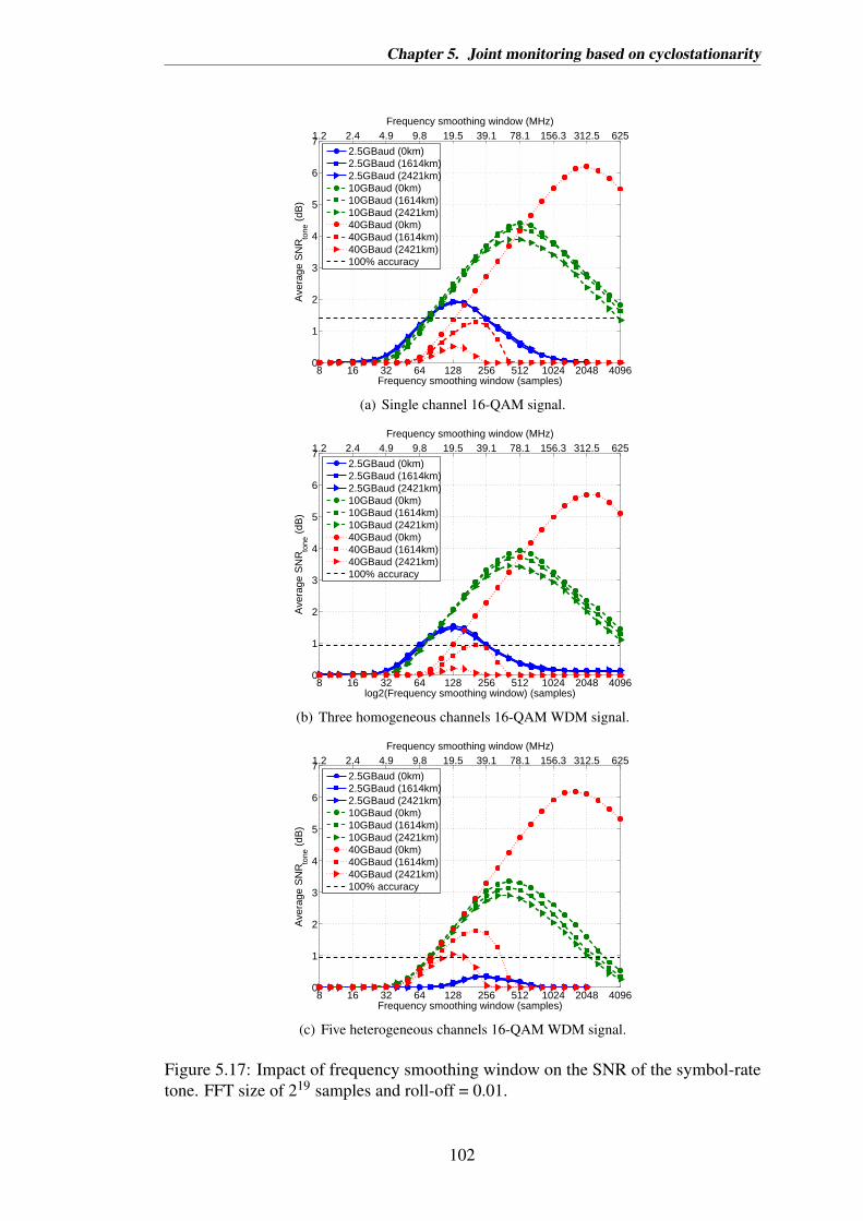
Chapter 5. Joint monitoring based on cyclostationarity
8 16 32 64 128 256 512 1024 2048 40960
1
2
3
4
5
6
7
Frequency smoothing window (samples)
Ave
rage
SN
Rto
ne (
dB)
1.2 2.4 4.9 9.8 19.5 39.1 78.1 156.3 312.5 625
Frequency smoothing window (MHz)
2.5GBaud (0km)2.5GBaud (1614km)2.5GBaud (2421km)10GBaud (0km)10GBaud (1614km)10GBaud (2421km)40GBaud (0km)40GBaud (1614km)40GBaud (2421km)100% accuracy
(a) Single channel 16-QAM signal.
8 16 32 64 128 256 512 1024 2048 40960
1
2
3
4
5
6
7
log2(Frequency smoothing window) (samples)
Ave
rage
SN
Rto
ne (
dB)
1.2 2.4 4.9 9.8 19.5 39.1 78.1 156.3 312.5 625
Frequency smoothing window (MHz)
2.5GBaud (0km)2.5GBaud (1614km)2.5GBaud (2421km)10GBaud (0km)10GBaud (1614km)10GBaud (2421km)40GBaud (0km)40GBaud (1614km)40GBaud (2421km)100% accuracy
(b) Three homogeneous channels 16-QAM WDM signal.
8 16 32 64 128 256 512 1024 2048 40960
1
2
3
4
5
6
7
Frequency smoothing window (samples)
Ave
rage
SN
Rto
ne (
dB)
1.2 2.4 4.9 9.8 19.5 39.1 78.1 156.3 312.5 625
Frequency smoothing window (MHz)
2.5GBaud (0km)2.5GBaud (1614km)2.5GBaud (2421km)10GBaud (0km)10GBaud (1614km)10GBaud (2421km)40GBaud (0km)40GBaud (1614km)40GBaud (2421km)100% accuracy
(c) Five heterogeneous channels 16-QAM WDM signal.
Figure 5.17: Impact of frequency smoothing window on the SNR of the symbol-ratetone. FFT size of 219 samples and roll-off = 0.01.
102

Chapter 5. Joint monitoring based on cyclostationarity
of channels is the noise floor of the SCF with respect to the cyclic frequency, whichincreases proportionally with the signal bandwidth, as Fig. 5.18 demonstrates. Despitethis SNR mismatch, there is no significant difference in terms of appropriate windowsize ranges, as the 100% accuracy threshold also increases proportionally by 0.4 dB. Aheterogeneous WDM setup which has a narrow central channel surrounded by widerchannels, such as 10-40-2.5-40-10 GBaud used in Fig. 5.17(c), will experience a shiftin the optimum average window, under the influence of the faster phase changes ofthe neighbouring channels, which will completely ’overshadow’ the symbol-rate tonecorresponding to the central channel. At the intersection of all three cases, the optimumwindow size is 128 samples, which will cover a wide range of rates and configurations,at the longest transmission distances allowed by the present technique.
When computing the SCF, we first compute the cyclic periodogram, which is initself an approximation to the analytical SCF (as explained in Section 3.3). Subsequently,a frequency smoothing stage reduces the inherent high variance of the periodogram andenhances the correlation between frequency components of the signal, by averagingout the contribution of the underlying random noise components - random in bothamplitude and phase. These contributions are twofold: impairments such as AWGNor laser phase noise on one hand, and the randomness of the data on the other hand.Because of this randomness, when α is not a multiple of the symbol-rate, the symbolsto be correlated are not in-phase and, this results in ’correlation noise’, which is simplyformed of random frequency components of the SCF.
A large smoothing window is required, such that through sufficient averaging, theSCF variation due to the presence of these noise components is reduced. The Grenader’sreliability condition (Eq. 3.25) can be observed here, as the window size must be muchgreater than unity. However, a too large window size will reduce the spectral correlation,as the phase components making up the average are dominated by noise, eventuallycovering the entire phase range (0,2π]. Spectrum broadening occurs, which means thatits phase and amplitude information is lost. A larger averaging window also means adecrease in computation speed. Therefore, a trade-off between a low variance and ahigh reliability, or a low computational effort and a high reliability must be attained(Fig. 5.19).
In a back-to-back transmission, the optimum frequency-smoothing window is ap-proximately equal to the bandwidth of the cyclic spectrum, as summarised in Table 5.4.Equivalently, the optimum number of symbols to be averaged by the moving averagefilter is equal to the number of symbols represented by the bandwidth of the cyclicspectrum, because that is the maximum number of symbols that can be correlated at onetime when α = Fb. The optimum window in number of symbols can be expressed as:
wopt(Symb) =Fb · r
Fs·Nsymb, (5.6)
103

Chapter 5. Joint monitoring based on cyclostationarity
0 10 20 30 40 50 60 70 80−140
−130
−120
−110
−100
−90
Cyclic frequency α (GHz)
SC
DF
(dB
m/H
z)
X−PolY−Pol
(a) 1 channel.
0 10 20 30 40 50 60 70 80−140
−130
−120
−110
−100
−90
Cyclic frequency α (GHz)
SC
DF
(dB
m/H
z)
X−PolY−Pol
(b) 2 channels.
0 10 20 30 40 50 60 70 80−140
−130
−120
−110
−100
−90
−80
Cyclic frequency α (GHz)
SC
DF
(dB
m/H
z)
X−PolY−Pol
(c) 3 channels.
0 10 20 30 40 50 60 70 80−140
−130
−120
−110
−100
−90
−80
Cyclic frequency α (GHz)
SC
DF
(dB
m/H
z)
X−PolY−Pol
(d) 4 channels.
0 10 20 30 40 50 60 70 80−140
−130
−120
−110
−100
−90
−80
Cyclic frequency α (GHz)
SC
DF
(dB
m/H
z)
X−PolY−Pol
(e) 5 channels.
0 10 20 30 40 50 60 70 80−130
−120
−110
−100
−90
−80
Cyclic frequency α (GHz)
SC
DF
(dB
m/H
z)
X−PolY−Pol
(f) 6 channels.
Figure 5.18: The SCF noise floor broadens proportionally with the number of channels.In this example, the channels are modulated at 16-QAM at 10 GBaud, spaced with noguard-band and filtered with a RRC roll-off of 0.1. There is no significant differencein the simulated SCF profile with respect to the cyclic frequency after the number ofchannels is increased beyond 5, due to the receiver bandwidth (24 GHz electrical).
where Fb and Fs are the symbol-rate and the sampling rate respectively, r is the roll-offand Nsymb is the total number of captured symbols.
If the capture time is restricted to say 3.28µs, 1.64µs or 0.82µs (equivalent toNFFT = 218, NFFT = 217 or NFFT = 216 FFT sample sizes respectively, when Fs =80 GSa/s), then the optimum window size (in number of samples) would changeappropriately to match the cyclic spectrum bandwidth, as summarised in Table 5.5and demonstrated in Figures 5.20 and 5.21. Whilst these latter results focus on thewindow size that maximises the tone SNR, a range of values around the optimum could
104

Chapter 5. Joint monitoring based on cyclostationarity
Too few averages:
Grenander's condition
(w>>1) is not met.
Optimum averages:
the entire
spectrum is included.
Too many averages:
noise components dominate,
leading to high variance
w w w
ASE noise phases
Signal phases
Signal phases+
Laser phase noise
Figure 5.19: Phases (top row) and amplitudes (bottom row) of the frequency componentsof a QPSK signal and noise, within one window, centred around 0 Hz. Choosing anoptimum number of averages is an important step in obtaining a reliable SCF estimateand therefore an accurate symbol-rate estimate.
Fb (GBaud) 2.5 10 40wopt (Samples) 27 29 211
wopt (MHz) 19.53 78.13 312.5Cyclic spectrum
bandwidth (MHz)25 100 400
Maximum distancebefore CD shifts the
wopt (km)
2,421 161.4 20
Maximum distancebefore ISI (km)
840 52.5 3.3
Table 5.4: Optimum averaging window in a back-to-back transmission, when 219
samples are processed and the roll-off factor is 0.01.
Fb (GBaud) 2.5 10 40wopt (Samples) 26 28 210
wopt (MHz) 19.53 78.13 312.5Cyclic spectrum
bandwidth (MHz)25 100 400
Table 5.5: Optimum averaging window in a back-to-back transmission, when 218
samples are processed and the roll-off factor is 0.01.
105

Chapter 5. Joint monitoring based on cyclostationarity
also allow 100% symbol-rate estimation accuracy. For instance, an FFT size of 218
samples and an averaging window size of 256 samples could also be used to estimate 10Gbaud and 40 GBaud. It becomes clear however, that lowering the number of capturedsamples has a great impact on the maximum transmission distance at 40 GBaud andthe lowest symbol-rates, as this limits the number of correlated symbols. As a result,at least 219 samples are required, in order to ensure that the technique proposed herecan successfully estimate the symbol-rate for a wider range of rates and transmissiondistances.
The optimum averaging window size decreases with an increase in distance (Fig.5.22), which is more noticeable for higher symbol-rates, more highly dependent on CD.By following the shift in optimum averaging window with distance, we can determinewhen the impact of CD becomes a limiting factor. The optimum window size cannot beselected per individual symbol-rate, as this is the unknown parameter to be estimated,thus a value that validates most cases must be selected.
In all of the following results in the remainder of this chapter, the investigationis restricted to a configuration of three homogeneous channels. In order to ensureoperation at the best spectral efficiency (lowest roll-off and highest symbol-rate) andlongest transmission distance, we assume 219 samples for processing and 128 samplesfor performing frequency averaging. Additionally, in order to lower the complexityof the algorithm, we assume that the symbol-rate is being restricted to 2.5 GBaud, 10GBaud and 40 GBaud, and typical FEC overheads (6.69−25% [Mizuochi, 2008]). Bycomputing the SCF only for cyclic frequencies within these restrictions, the complexityof the estimator is greatly reduced. If very low symbol-rates, such as 2.5 GBaud, areunlikely, then averaging every 258 samples over a total 218 captured samples would bemore advantageous, such that longer distances and higher rates could be supported.
Impact of chromatic dispersion
In order to more thoroughly investigate the impact of chromatic dispersion on theproposed joint-estimation technique, we look at the SNR of the tone at the symbol-rateas a function of the traversed length of fibre. We find that the power of Sα=Fb
y ( f ) isstrongly dependent on the amount of accumulated CD, as Fig. 5.23 shows.
As the different frequency components of the signal experience different propagationspeeds through the fibre, their different arrival times at the receiver translates into thefrequency domain as a frequency-dependent phase shift. The frequency componentsseparated by the symbol-rate value are no longer in-phase, therefore their correlationis reduced. Sα=Fb
y ( f ) will fade with dispersion, eventually falling into the noise floorand the loss of periodicity in the SCF, can be coined as ’spectral correlation fading’.As a result, the symbol-rate estimation based on the SCF approach is limited by theamount of cumulative dispersion present in the path of the signal, but will continue to
106

Chapter 5. Joint monitoring based on cyclostationarity
8 16 32 64 128 256 512 1024 20480
1
2
3
4
5
6
7
log2(Frequency smoothing window) (samples)
Ave
rage
SN
Rto
ne (
dB)
2.4 4.9 9.8 19.5 39.1 78.1 156.3 312.5 625
Frequency smoothing window (MHz)
2.5GBaud (0km)2.5GBaud (1614km)2.5GBaud (2421km)10GBaud (0km)10GBaud (1614km)10GBaud (2421km)40GBaud (0km)40GBaud (1614km)40GBaud (2421km)100% accuracy
(a) NFFT = 218 samples.
8 16 32 64 128 256 512 1024 20480
1
2
3
4
5
6
7
log2(Frequency smoothing window) (samples)
Ave
rage
SN
Rto
ne (
dB)
4.9 9.8 19.5 39.1 78.1 156.3 312.5 625 1250
Frequency smoothing window (MHz)
2.5GBaud (0km)2.5GBaud (1614km)2.5GBaud (2421km)10GBaud (0km)10GBaud (1614km)10GBaud (2421km)40GBaud (0km)40GBaud (1614km)40GBaud (2421km)100% accuracy
(b) NFFT = 217 samples.
8 16 32 64 128 256 512 1024 20480
1
2
3
4
5
6
7
log2(Frequency smoothing window) (samples)
Ave
rage
SN
Rto
ne (
dB)
9.8 19.5 39.1 78.1 156.3 312.5 625 1250 2500
Frequency smoothing window (MHz)
2.5GBaud (0km)2.5GBaud (1614km)2.5GBaud (2421km)10GBaud (0km)10GBaud (1614km)10GBaud (2421km)40GBaud (0km)40GBaud (1614km)40GBaud (2421km)100% accuracy
(c) NFFT = 216 samples.
Figure 5.20: Impact of frequency smoothing window on the SNR of the symbol-ratetone for three 16-QAM channels, different FFT sizes and a fixed roll-off = 0.01.
107

Chapter 5. Joint monitoring based on cyclostationarity
13 14 15 16 17 18 19 20 21 22 231248
163264
128256512
102420484096
log2(NFFT
) (samples)
Opt
imum
ave
ragi
ng w
indo
w (
sam
ples
)
2.5GBaud, 0km10GBaud, 0km40GBaud, 0km100% accuracy limit
Figure 5.21: The optimum frequency-smoothing window for a maximum SNR of thesymbol-rate tone, at different FFT sizes, a fixed roll-off of 0.01 and a sampling rate of80 GSa/s. Back-to-back simulation of DP-16QAM signals.
0 10 100 1,000 10,000 100,00064
128
256
512
1024
2048
Distance (km)
Fre
quen
cy s
moo
thin
g w
indo
w (
sam
ples
)
2.5 GBaud 10 GBaud 40 GBaud
Figure 5.22: Optimum frequency smoothing window as a function of distance, in asimulated WDM signal formed of three homogeneous 16-QAM channels. The hollowmarkers indicate the maximum distance for which the estimation accuracy is 100%.
work without CD compensation until complete spectral correlation fading occurs, whenthe symbol-rate tone will no longer be distinguishable from the correlation noise floor.By contrast, in order to be able to apply the OSNR estimation technique effectively, CDestimation and compensation will be required a priori, because the signal power willfade with distance, leading to the OSNR to be underestimated. This aspect is discussedin more detail in the following Subsection 5.7.
Figure 5.24 shows the maximum achievable distances for estimating the symbol-ratewith 100% accuracy, depending on the number of samples in the averaging window.
108

Chapter 5. Joint monitoring based on cyclostationarity
0 5,000 10,000 15,000 20,000 25,0000
0.5
1
1.5
2
2.5
3
3.5
Distance (km)
SN
Rto
ne (
dB)
RRC roll−off=0.01RRC roll−off=0.1RRC roll−off=0.5
0
9899.7
100
Acc
urac
y (%
)
RRC roll−off=0.01RRC roll−off=0.1RRC roll−off=0.5
(a) 10 GBaud,16-QAM
0 5,000 10,000 15,000 20,000 25,0000
0.5
1
1.5
2
2.5
3
3.5
Distance (km)
SN
Rto
ne (
dB)
RRC roll−off=0.01RRC roll−off=0.1RRC roll−off=0.5
0
93.799.3
100
Acc
urac
y (%
)
RRC roll−off=0.01RRC roll−off=0.1RRC roll−off=0.5
(b) 10 GBaud,QPSK
0 5,000 10,000 15,000 20,000 25,0000
0.5
1
1.5
2
2.5
3
3.5
Distance (km)
SN
Rto
ne (
dB)
RRC roll−off=0.01RRC roll−off=0.1RRC roll−off=0.5
0
92.7
98.7
100
Acc
urac
y (%
)
RRC roll−off=0.01RRC roll−off=0.1RRC roll−off=0.5
(c) 40 GBaud, 16-QAM
0 5,000 10,000 15,000 20,000 25,0000
0.5
1
1.5
2
2.5
3
3.5
Distance (km)
SN
Rto
ne (
dB)
RRC roll−off=0.01RRC roll−off=0.1RRC roll−off=0.5
0
93.796
100
Acc
urac
y (%
)
RRC roll−off=0.01RRC roll−off=0.1RRC roll−off=0.5
(d) 40 GBaud, QPSK
Figure 5.23: Impact of chromatic dispersion on the SCF tone SNR and symbol-rateestimation demonstrated by simulation.
109

Chapter 5. Joint monitoring based on cyclostationarity
At high values of the RRC roll-off, such as 0.1 or 0.5, the spectral correlation is moreeasily achieved, enabling high reach for various window sizes. As the roll-off factordecreases, the spectral correlation is reduced, limiting the range of acceptable averagingwindow sizes. For the maximum spectral efficiency case considered, when the roll-offis 0.01 and the symbol-rate is 40 GBaud, the optimum window size is approximately203 samples, enabling the estimator to operate even after the superchannel has travelledover 1614 km of fibre. However, the reach can be at least doubled if a higher roll-offis used. There is therefore a trade-off between spectral-efficiency and reach in termsof the performance of this symbol-rate estimation method, just as it is in terms of thegeneral DSP performance for such signals.
102
103
104
105
106
4
5
6
7
8
9
10
Maximum reach for 100% accuracy (km)
log2
(Mov
ing−
aver
age
win
dow
siz
e) (
sam
ples
)
roll−off=0.01roll−off=0.1roll−off=0.5
40 GBaud 10 GBaud 2.5 GBaud
Figure 5.24: Maximum achievable distance limited by the accuracy of the symbol-rateestimation, by simulating three-channel 16-QAM WDM signals, without linear ICI.
Impact of Nyquist pulse shaping
Assuming that the transmission distance is fixed, we are then interested in maximisingthe spectral efficiency. Testing by simulation and experimentally, for both 16-QAMand QPSK, the minimum RRC roll-off for ensuring a perfect symbol-rate estimationhas been determined. As Fig. 5.25 shows, higher transmission distances impose amore stringent requirement on the spectral efficiency with this estimation technique.Over 2017.5 km with QPSK modulation, the minimum roll-off factor is 0.008, whilefor the shorter distance of 807 km with 16-QAM, the minimum roll-off is 0.006.
110

Chapter 5. Joint monitoring based on cyclostationarity
Experimentally, when there is no dispersion, these results confirm that a roll-off as lowas 0.01 allows a correct symbol-rate estimation. At even lower roll-offs the discrepancybetween simulation and experimental results can be attributed to further signal powerlosses, present in the experiment, but unaccounted for in the simulation.
0.001 0.01 0.1 10
20
40
60
80
100S
ymbo
l−ra
te e
stim
atio
n ac
cura
cy (
%)
Root−raised cosine roll−off
Simulation 0 kmSimulation 807 kmExperiment 0 km
(a) QPSK.
0.001 0.01 0.1 10
20
40
60
80
100
Sym
bol−
rate
est
imat
ion
accu
racy
(%
)
Root−raised cosine roll−off
Simulation 0 kmSimulation 807 kmExperiment 0 km
(b) 16-QAM.
Figure 5.25: Impact of RRC roll-off on the symbol-rate estimation, in a three channelWDM signal, modulated with 16-QAM at 10 GBaud.
111

Chapter 5. Joint monitoring based on cyclostationarity
Independence of OSNR
While the symbol-rate estimation limits have been investigated so far assuming linearregime operation, here we investigate the impact of highly linear and non-linear noiseon the symbol-rate estimator. The simulations parameters assumed are described below.
λ [nm] 1550α [dB
km ] 0.2D [ ps
nm·km ] 16.78S [ ps
nm2·km ] 0.06PMD parameter [ ps√
km] 0.1
γ [ 1W ·km ] 1.2
Split step size [km] 0.5Span length [km] 80.7Number of spans 10 / 25
Table 5.6: Fibre parameters used in simulating the impact of OSNR on the symbol-rateestimation.
An important advantage of the SCF method for symbol-rate estimation is that it iscompletely independent of linear and non-linear noise, as demonstrated by simulationand experimentally in Fig. 5.26. This is due to the fact that noise can be modelled as awide-sense stationary, but not cyclostationary, process which means that the spectralcorrelation of noise is not periodic and thus does not generate correlation peaks atnon-zero cyclic frequencies.
0 5 10 15 20 25 30 359
9.2
9.4
9.6
9.8
10
10.2
10.4
10.6
10.8
11
OSNR0.1nm
(dB)
Estim
ate
d s
ym
bol
rate
(G
Baud)
16 QAM 807km (Sim )
16
QP
QP
Figure 5.26: Symbol-rate estimation independence of the OSNR, in a three channel 10GBaud WDM signal.
112

Chapter 5. Joint monitoring based on cyclostationarity
5.3.2 Cyclic autocorrelation function approach
The time-domain implementation of the cyclostationarity-based symbol-rate estimatorutilises the CAF, as Fig. 5.27 depicts. Compared to the frequency-domain implementa-tion of Fig. 5.10, to which it is almost identical, the time-domain implementation doesnot employ a moving average filter, but instead uses an IFFT to translate the spectralcorrelation back into the time-domain. For a given cyclic frequency α, the CAF of areceived signal y(t) is the IFFT of its cyclic periodogram at α:
Rαy (τ) =
Z∞
−∞
Y(
f +α
2
)·Y ∗(
f − α
2
)· e j2π f τd f (5.7)
A more detailed explanation of the relationship between the CAF and the cyclic peri-odogram as a Fourier Transform pair, can be found in Chapter 3. The IFFT is in itself afrequency-smoothing stage, because it is the average at time τ of all complex frequencycomponents of the spectrum Y ( f ), that are separated by α. This alternative time-domainimplementation has a significant impact on the performance of the symbol-rate estimatoras a function of dispersion, as well as roll-off factor, as it will be demonstrated next. Interms of processing speed, the replacement of the moving average operation by an IFFToperation does not change the complexity of the algorithm, as explained in Section 5.2.
x(t) Fb
NFFT
*Rx(τ)
ejπαnt
e-jπαnt
NFFT
FFT
FFT
NFFT
αnFFT
I
NFFT
*Rx(τ)
ejπα1t
e-jπα1t
NFFT
FFT
FFT
NFFT
α1FFT
IRx(τ)
αargα≠0maxmaxf
Figure 5.27: Implementation of the symbol-rate estimation algorithm based on the CAF.
After the CAF is computed for a selection of cyclic frequencies, its tones profileis obtained by taking the highest cyclic autocorrelation values along the time-lags τ
for each cyclic frequency α. The result is a two-dimensional profile from the three-dimensional CAF, as in Fig. 5.28(b) for a homogeneous WDM signal or Fig. 5.28(d)for a heterogeneous WDM signal. The profile can be called the CAF tones function for
113

Chapter 5. Joint monitoring based on cyclostationarity
the received signal y(t) and is defined with respect to the cyclic frequency as:
Ty,CAF(α) = maxτ≥0
∣∣Rαy (τ)
∣∣ , (5.8)
It is important to note that the causality condition τ≥ 0 is imposed on this measurement.The symbol-rate estimate is then simply the non-zero cyclic frequency corresponding tothe maximum tone:
Fb = argα6=0 maxTy,CAF(α). (5.9)
Similarly to the symbol-rate estimation based on the SCF, single tones or multipletones appear in the CAF of WDM signals, depending on whether they are homogeneousor multi-rate heterogeneous (Fig. 5.28).
As explained in Section 3.1, the CAF of linearly modulated signals, such as QPSKor 16-QAM, contains harmonics of a fundamental frequency equal to the symbol-rate.If any type of low pass filtering is applied on the signal, then the highest harmonicswill reduce to zero and only the fundamental frequency will typically remain. Thesetheoretical characteristics can be observed indeed in Fig. 5.28(b), showing the profileof the CAF with respect to the cyclic frequency α, for a WDM signal formed of threechannels, each modulated with 16-QAM at 10 GBaud symbol-rate and RRC filtered witha roll-off factor of 0.5. The two highest peaks correspond to the cyclic frequencies equalto zero and the symbol-rate (the Direct Current (DC) and the fundamental frequencycomponents respectively). The higher harmonics (20 GHz, 30 GHz, 40 GHz etc.) arenot appearing, as they are strongly filtered by the RRC filter at the transmitter. At allother cyclic frequencies, not integer multiples of the symbol-rate α 6= k ·Fb, k ∈ Z, theCAF is approximately zero, as expected.
This proposed technique also works for heterogeneous WDM configurations, suchas the one shown in Fig. 5.28(c), for three channels modulated with 2.5 GBaud 64-QAM, 25 GBaud QPSK and 10 GBaud 16-QAM respectively. The OSNR matches theaverage ROSNR across all channels, assuming a FEC limit of 3.8 ·10−3. In these results,the launch power per channel is set out to be directly proportional to the symbol-rate,such that to maximise the individual transmission distances [Poggiolini et al., 2011].Consequently, we find that the correlation tones increase in power with the channelbandwidth, suggesting that wider bandwidths correlate better under this technique. Eventhough the correspondence between the channel rate and channel location is lost, thisinformation could be recovered through further DSP, but this aspect is not investigatedin this thesis.
In this section, the time-domain approach to the cyclostationarity-based symbol-rateestimator is investigated with respect to ranges of rates that can be accurately estimated,the RRC excess bandwidth and CD.
114

Chapter 5. Joint monitoring based on cyclostationarity
−40 −30 −20 −10 0 10 20 30 40−130
−120
−110
−100
−90
−80
−70
Frequency (GHz)
PS
D (
dBm
/Hz)
X−PolY−Pol
(a) Power Spectral Density.
0 10 20 30 40 50 60 70 800
0.2
0.4
0.6
0.8
1
Cyclic frequency (GHz)
Nor
mal
ised
cyc
lic c
orre
latio
n
10GBaud 16−QAM
(b) Profile of the Cyclic Autocorrelation Function.
−40 −30 −20 −10 0 10 20 30 40−130
−120
−110
−100
−90
−80
−70
Frequency (GHz)
PS
D (
dBm
/Hz)
X−PolY−Pol
(c) Power Spectral Density.
0 10 20 30 40 50 60 70 800
0.2
0.4
0.6
0.8
1
Cyclic frequency (GHz)
Nor
mal
ised
cyc
lic c
orre
latio
n
2.5GBaud 64−QAM25GBaud QPSK10GBaud 16−QAM
(d) Profile of the Cyclic Autocorrelation Function.
Figure 5.28: The Cyclic Autocorrelation Function of a homogeneous WDM signalspectrum (a) has a single tone (b), whilst a heterogeneous WDM signal spectrum (c)has multiple tones (d), one for each individual symbol-rate. Simulation and processingof 219 samples; RRC roll-off factor of 0.5.
Range and accuracy
A robust symbol-rate estimator requires 100% accuracy over a wide range of values,such that it can be used with both established and future optical transmission systemconfigurations. Fig. 5.29 depicts the estimation range for a configuration of threecontiguous channels, modulated with 16-QAM and pulse shaped with a RRC filter of1%, 10% and 50% excess bandwidths, in turn. After an ideal transmission (dispersion-and nonlinearity-free), the signals are noise-loaded at the receiver such that the OSNRmatches the ROSNR for a FEC requirement of 3.8 ·10−3 at the corresponding symbol-rate. These ROSNR values can be found in Fig. 2.3. Again, the IF between LO andtransmitter lasers is randomly selected within the interval [−1GHz,1GHz], values asobserved in practice, to justify the independence of this technique on typical frequencyoffset variations. The tested symbol-rate values are between 1 and 70 GBaud, in stepsof 1 GBd, whilst the cyclic frequencies are between 0 and 80 GHz in steps of 500 MHz.
115

Chapter 5. Joint monitoring based on cyclostationarity
0 10 20 30 40 50 60 700
10
20
30
40
50
60
70
80
90
100
Symbol−rate (Gbaud)
Est
imat
ed s
ymbo
l−ra
te a
ccur
acy
(%)
roll−off=0.01roll−off=0.1roll−off=0.5
Figure 5.29: Range and accuracy of symbol-rate estimation based on the Cyclic Auto-correlation Function. Three channels modulated with 16-QAM, simulated back-to-backand sampled at 80 GSa/s for 6.55 µs (219 captured samples).
The results show that the symbol-rate can be estimated over a wide range of values,even exceeding the receiver’s cutoff and Nyquist frequencies. Such a performance canbe better explained visually, by examining the shape of the tones profile at differentsymbol-rates in Fig. 5.31. Here, the CAF tones are normalised to the DC componentand expressed in dBs:
Ty,CAF(α)[dB]−Ty,CAF(0)[dB] = 10 log10
(maxτ≥0
∣∣Rαy (τ)
∣∣maxτ≥0
∣∣R0y(τ)
∣∣)
[dB] (5.10)
When the roll-off is 10% the maximum symbol-rate that can be estimated with 100%accuracy is 52 GBaud. Up to this value, the tone corresponding to the symbol-rate(α = Fb), is easily detectable for this particular roll-off factor, as it lies above all othercyclic frequencies (with the exception of the DC) forming a ’correlation noise floor’.The shape of the CAF profile is influenced by the signal configuration, but also by anytype of filtering that the signal has undergone, including the RRC at the transmitter orthe Low-Pass Filter (LPF) at the receiver, for instance. When the symbol-rate increasesbeyond 52 GBaud, the correlation is still achieved, but the tone power is lower as aresult of low-pas filtering, which attenuates higher frequencies.
Fig. 5.30 demonstrates that for the same set of symbol-rates the tone power increasesas the roll-off is increased to 0.5. For example, the tone at 52 GBaud has a much higherSNR when the roll-off is 0.5 compared to roll-off of 0.1. As a consequence, theestimation range extends up to 59 GBaud, because wider bandwidths increase thecorrelation at α = Fb.
116

Chapter 5. Joint monitoring based on cyclostationarity
0 10 20 30 40 50 60 70 80−60
−50
−40
−30
−20
−10
0
Cyclic frequency (GHz)
Nor
amal
ised
CA
F (
dB)
2.5 GBaud 16−QAM
(a)
0 10 20 30 40 50 60 70 80−60
−50
−40
−30
−20
−10
0
Cyclic frequency (GHz)
Nor
amal
ised
CA
F (
dB)
10.7 GBaud 16−QAM
(b)
0 10 20 30 40 50 60 70 80−60
−50
−40
−30
−20
−10
0
Cyclic frequency (GHz)
Nor
amal
ised
CA
F (
dB)
32 GBaud 16−QAM
(c)
0 10 20 30 40 50 60 70 80−60
−50
−40
−30
−20
−10
0
Cyclic frequency (GHz)
Nor
amal
ised
CA
F (
dB)
40 GBaud 16−QAM
(d)
0 10 20 30 40 50 60 70 80−60
−50
−40
−30
−20
−10
0
Cyclic frequency (GHz)
Nor
amal
ised
CA
F (
dB)
52 GBaud 16−QAM
100% accuracy limit
(e)
0 10 20 30 40 50 60 70 80−60
−50
−40
−30
−20
−10
0
Cyclic frequency (GHz)
Nor
amal
ised
CA
F (
dB)
70 GBaud 16−QAM
100% accuracy limit
(f)
Figure 5.30: Normalised Cyclic Autocorrelation Function, for three contiguous WDMsimulated channels, and a wide selection of symbol-rates (RRC roll-off factor is 0.5).
117

Chapter 5. Joint monitoring based on cyclostationarity
0 10 20 30 40 50 60 70 80−60
−50
−40
−30
−20
−10
0
Cyclic frequency (GHz)
Nor
amal
ised
CA
F (
dB)
2.5 GBaud 16−QAM
(a)
0 10 20 30 40 50 60 70 80−60
−50
−40
−30
−20
−10
0
Cyclic frequency (GHz)
Nor
amal
ised
CA
F (
dB)
10.7 GBaud 16−QAM
(b)
0 10 20 30 40 50 60 70 80−60
−50
−40
−30
−20
−10
0
Cyclic frequency (GHz)
Nor
amal
ised
CA
F (
dB)
32 GBaud 16−QAM
(c)
0 10 20 30 40 50 60 70 80−60
−50
−40
−30
−20
−10
0
Cyclic frequency (GHz)
Nor
amal
ised
CA
F (
dB)
40 GBaud 16−QAM
(d)
0 10 20 30 40 50 60 70 80−60
−50
−40
−30
−20
−10
0
Cyclic frequency (GHz)
Nor
amal
ised
CA
F (
dB)
52 GBaud 16−QAM
100% accuracy limit
(e)
0 10 20 30 40 50 60 70 80−60
−50
−40
−30
−20
−10
0
Cyclic frequency (GHz)
Nor
amal
ised
CA
F (
dB)
70 GBaud 16−QAM
100% accuracy limit
(f)
Figure 5.31: Normalised Cyclic Autocorrelation Function, for three contiguous WDMsimulated channels, and a wide selection of symbol-rates (RRC roll-off factor is 0.1).
118

Chapter 5. Joint monitoring based on cyclostationarity
Conversely, for very low excess bandwidths such as 1%, the correlation peakdisappears (Fig. 5.32), as the bandwidth is insufficient to obtain a strong overlapbetween the two shifted copies of the spectra. Referring back to Fig. 5.29, in thiscase, the technique completely fails for the entire range of symbol-rates. Therefore, theroll-off factor strongly limits this symbol-rate estimation approach, which is studied inmore detail in the following section.
0 10 20 30 40 50 60 70 80−60
−50
−40
−30
−20
−10
0
Cyclic frequency (GHz)
Nor
amal
ised
CA
F (
dB)
10.7 GBaud 16−QAM
(a)
0 10 20 30 40 50 60 70 80−60
−50
−40
−30
−20
−10
0
Cyclic frequency (GHz)
Nor
amal
ised
CA
F (
dB)
40 GBaud 16−QAM
(b)
Figure 5.32: Normalised Cyclic Autocorrelation Function, for three contiguous WDMsimulated channels, and a wide selection of symbol-rates (RRC roll-off factor is 0.01).
Whilst in the previous example, the symbol-rate value was always found in therange of cyclic frequencies under test, in a real-time application assuming arbitrarysymbol-rates, it may be necessary to scan the spectrum over even a finer cyclic frequencygranularity, in order to ensure that the symbol-rate tone is correctly identified. It isnot necessary to have an exact match between the set of possible symbol-rates andthe set of tested values, as correlation can still occur even for a small offset of theorder of kHz. If, Fb is the value to be estimated, let ∆αmax = α−Fb be the maximumcyclic frequency step size deviation from Fb, allowed before the correlation is lost.For any cyclic frequency granularity greater than ∆αmax, the symbol-rate tone can beundetectable, by the scanning process.
The measurement precision is thus quantified as the power ratio between the spectraltone at an arbitrary α and the spectral tone at the known symbol-rate:
Ty,CAF(α)[dB]−Ty,CAF(Fb)[dB] = 10 log10
maxτ≥0
∣∣∣CFb+∆αy (τ)
∣∣∣maxτ≥0
∣∣∣RFby (τ)
∣∣∣ . (5.11)
Fig. 5.33 shows the precision measurements and that ∆αmax = 208 kHz for 10%excess bandwidth, an exact match with the SCF precision. If the roll-off is 0.01, thena careful selection of the cyclic frequency granularity is futile, as the estimation isinaccurate in all cases. For low symbol-rates, such as 2.5 GBaud or 10 GBaud, there
119

Chapter 5. Joint monitoring based on cyclostationarity
is no clear difference between the tone at exactly the symbol-rate and the tones within±1 MHz from it. When the symbol-rate is 40 GBaud, there is correlation betweenfrequency components in a narrow range around Fb (or around ∆α = 0) because theincrease in channel bandwidth, as previously discussed. However, this correlation doesnot yield a sufficiently high power tone to be detected by the estimator, as it is in factclear from Fig. 5.32(b).
−1 −0.5 0 0.5 1−0.8
−0.6
−0.4
−0.2
0
0.2
∆α (MHz)
Ton
e at
α r
elat
ive
to th
e ba
ud to
ne (
dB)
2.5 GBaud10 GBaud40 GBaud
(a) 0.01 roll-off
−1 −0.5 0 0.5 1−10
−8
−6
−4
−2
0
2
∆α (MHz)
Ton
e at
α r
elat
ive
to th
e ba
ud to
ne (
dB)
208kHz
2.5 GBaud10 GBaud40 GBaud
(b) 0.1 roll-off
Figure 5.33: Precision of the symbol-rate estimation technique based on the CAFdemonstrated by simulation for DP-16QAM. 219 samples are processed and onlyAWGN is assumed as impairment.
Impact of Nyquist pulse shaping
The narrowing of the signal spectrum when employing Nyquist pulse shaping corre-sponds to the broadening of the pulse in the time domain. In turn, this broadening resultsin a lower CAF tone power, leading to a trade-off between the temporal correlation andspectral efficiency. Fig. 5.34(a), which depicts the measurement of the peak power inthe estimated tone relative to the noise floor,
SNRtone = 10 log10maxτRFb
y (τ)maxRα 6=Fb
y (τ), (5.12)
demonstrates that the correlation changes proportionally with the roll-off, as wellas the symbol-rate. For the three different symbol-rates considered, the SNR of thesymbol-rate tone is identically zero for roll-offs of 0.018 and lower, when the temporalcorrelation cannot be achieved. However, on average, the tone power needs to exceed0.7 dB in order for 100% estimation accuracy to be guaranteed.
As the symbol-rate increases, the range of roll-offs supported by the technique alsoincreases. Fig. 5.34(b) confirms that the minimum roll-offs to correctly estimate 2.5GBaud, 10 GBaud and 40 GBaud are approximately 0.056, 0.032 and 0.024 respec-
120

Chapter 5. Joint monitoring based on cyclostationarity
0.001 0.01 0.1 0.5 10
0.7
5
10
15
Root−raised cosine roll−off
SN
Rto
ne (
dB)
2.5 GBaud10 GBaud40 GBaud
100% accuracy
(a)
0.001 0.01 0.1 0.5 10
20
40
60
80
100
Root−raised cosine roll−off
Sym
bol−
rate
est
imat
ion
accu
racy
(%
)
2.5 GBaud (Sim.)10 GBaud (Sim.)40 GBaud (Sim.)10 GBaud (Exp.)
(b)
Figure 5.34: Impact of the RRC filter on the CAF-based symbol-rate estimation in termsof SNR of the estimated tone (a) and accuracy (b), when AWGN is the only impairment.
tively. When the roll-off approaches unity, the SNRtone of 40 GBaud is lowered, asthe bandwidth of the signal is more strongly filtered at the receiver compared to thelower rates. Experimentally it was found that the minimum roll-off for estimating 10GBaud, in a back-to-back transmission, is in fact 0.07. The slight difference betweenthe experimental and simulation findings can be attributed to further possible losses inthe signal path, unaccounted for in simulation, which reduce the tone’s SNR.
These results suggest that with the presented technique it is by far more advantageousto increase the spectral efficiency by increasing the symbol-rate, whilst keeping a roll-offfactor greater than 0.07. This is in fact the opposite requirement to the predicted trendin the design of future fast optical networks.
121

Chapter 5. Joint monitoring based on cyclostationarity
Impact of chromatic dispersion
CD limits the maximum achievable transmission distances, as the pulses spread quadrat-ically with the symbol-rate, leading to ISI. To limit this effect, a low RRC roll-offis preferred. However as described previously, a too low roll-off will limit the cyclicautocorrelation tone power, until complete fading when this value is approaching zero,as RRC filtering dissipates the energy in the CAF tones along the time-lag (Section 3.4,Figure 3.17).
In Figure. 5.35, we observe that the SNR of the fundamental cyclic frequency(α = Fb) decreases slowly with distance, in particular for lower symbol-rates, and that aroll-off of 0.01 is detrimental to the estimation. As the symbol-rate is increased, the CDimpact is higher, however the SNR tone is still decreasing at a slow rate. As the roll-offfactor is increased, the method becomes even less affected by accumulated dispersion,because the tone SNR is higher.
103
104
105
1060
5
10
15
20
Length (km)
SN
Rto
ne (
dB)
roll−off = 0.01roll−off = 0.1roll−off = 0.5
(a) 2.5 GBaud, 3 channels 16-QAM.
103
104
105
1060
5
10
15
20
Length (km)
SN
Rto
ne (
dB)
roll−off = 0.01roll−off = 0.1roll−off = 0.5
(b) 10 GBaud, 3 channels 16-QAM.
103
104
105
1060
5
10
15
20
Length (km)
SN
Rto
ne (
dB)
roll−off = 0.01roll−off = 0.1roll−off = 0.5
(c) 40 GBaud, 3 channels 16-QAM.
Figure 5.35: Impact of CD on the CAF-based symbol-rate estimation by simulation.
Due to this slow SNR decrease, the symbol-rate estimation based on the CAFappears as if it is CD independent, since it can function with 100% reliability fortransmission distances of at least 173,500 km, as in Fig. 5.35(c) for instance when
122

Chapter 5. Joint monitoring based on cyclostationarity
the roll-of is 0.1 and the symbol-rate is 40 GBaud. From a practical point of view, assuch high distances are not traversed without regeneration, it can be assumed that thisestimator is indeed CD independent.
5.3.3 Comparison between the time domain and frequency domainsymbol-rate estimators
Selecting the best between the two investigated techniques involves a few practicalconsiderations. The optimum symbol-rate estimation technique performs with 100%accuracy for the highest transmission distance at the highest spectral efficiency and canallow a wide range of symbol-rates to be estimated. Ideally, fibre impairments shouldhave minimal or no impact on the estimator. Between two estimators that are matchingin performance, the one requiring the lowest computational effort is preferred.
The time-domain approach has a more stringent lower-bound limit on the excessbandwidth, imposing stricter requirements on the transmission configuration, suchthat this technique could be employed at the receiver. Although the IFFT employedto compute the CAF is a type of averaging operation, the moving-average filter is amuch better frequency smoothing stage for enhancing the correlation when the signalbandwidth approaches Nyquist, as it has been demonstrated to work for roll-offs of0.01.
On the other hand, since frequency-smoothing is not performed, the impact of CDon the CAF is reduced compared to the SCF. At sufficiently high roll-off factors, theSNRtone is improved, as the peak at the cyclic frequency equal to the symbol-rate isbetter defined compared to the SCF method. For example, when the symbol-rate was10 GBaud, the tones SNR of the CAF decrease at a much lower rate of approximately0.05 dB in 21,793 km, compared to the tones of the SCF which decrease approximatelyexponentially, starting at only 3.2 dB above the noise floor and dropping to 0 dB in20,000 km.
The spectral efficiency is defined as the capacity that can be transmitted in a unitbandwidth. For any M-arry dual-polarised modulation format, either single channel orcontiguous superchannels configuration, it is given by:
SE =Nch ·2log2 M ·Fb
Nch ·Fb · (1+ r)=
2log2 M(1+ r)
. (5.13)
In other words, for these particular cases, the spectral efficiency is actually indepen-dent on the symbol-rate or number of channels, and can be maximised by increasingthe modulation format order, decreasing the roll-off or both. Assuming DP-16QAMas the modulation format of choice, we compare the two cyclostationary symbol-rateestimation approaches in terms of the maximum spectral efficiency that they can support
123

Chapter 5. Joint monitoring based on cyclostationarity
and find a 0.4 b/s/Hz difference in the favour of the frequency domain approach.Some of the performance limitations discussed thus far in this section, are sum-
marised in Table 5.7.
Frequency-domain (SCF) Time-domain (CAF)Maximum symbol-rate (GBaud)
r=0.01 r=0.1 r=0.541.8 45.4 45.65
r=0.01 r=0.1 r=0.50 52 59
Maximum distance (km) as a function of the symbol-rate, Fb (GBd)Fb r=0.01 r=0.1 r=0.52.5 48,420 129,120 128,47410 9,684 22,596 26,71240 1,614 3,228 3,470
Fb r=0.01 r=0.1 r=0.52.5 0 >798,900 >798,90010 0 782,800 >798,90040 0 173,500 242,100
Minimum RRC roll-off when the symbol-rate is 10 GBaudr=0.01 r =0.07
Maximum spectral efficiency (b/s/Hz)7.9 (M=16, r=0.01) 7.5 (M=16, r=0.07)
Complexity2CNADClog2(NADC) 3CNADClog2(NADC)
Table 5.7: Performance of the SCF- and CAF-based symbol-rates estimators, for threecontiguous WDM channels, modulated with DP-16QAM.
Selecting which one the two estimators will be used, depends on the application. Interms of complexity they are comparable. The time-domain technique performs betterin terms of CD to the detriment of limiting the lowest allowed roll-off. As a result, formost optical communications applications, the SCF approach would be preferred, asit allows the estimation of the symbol-rate over the widest range of roll-offs, and forreasonably high transmission distances.
5.4 Roll-off estimation
The RRC roll-off factor can be additionally estimated from the CAF computation, bylooking at the power ratio between the tone at the symbol-rate and the DC. This ratiowill be linear for a wide range of roll-offs, as shown in Fig. 5.36. Finding this linearapproximation in a transceiver self-configuration stage, could thus enable the estimationof the roll-off factor with an acceptable performance [Yang et al., 2009] of < 20% RootMean Squared Error (RMSE) down to a roll-off of 0.06, as demonstrated in Fig. 5.37.
These results have been investigated in a back-to-back transmission setup, in thepresence of AWGN, loaded at the receiver to give the ROSNR for FEC = 3.8 · 10−3.When pulse shaping is approaching the Nyquist limit, the symbol-rate tone becomesindistinguishable from the correlation noise floor, resulting in slight increases in errors
124

Chapter 5. Joint monitoring based on cyclostationarity
for roll-offs below 0.06. The discrepancy between the simulation and the experimentalresults in the low roll-off region arises from the additional noise sources that are presentin the experiment but not accounted for in the simulation. On the other hand, whenthe signal bandwidth is higher than the receiver bandwidth, the tone power is alsodiminished, as the channel is being filtered out. The receiver bandwidth limitation isevident in particular at 40 GBaud, when the roll-off is greater than 0.3. As a consequence,this estimator will perform well, as long as the signal bandwidth is not strongly filtered.
The CAF of cyclostationary signals, computed as in Section 5.2, is only slowlyfading with dispersion (Section 5.3.2). In fact, the SNR of the symbol-rate tone isapproximately constant up to 18,000 km for a wide range of rates and roll-off factors(0.06-0.3), as it has been shown in Fig. 5.35. It is therefore expected that this techniqueshould also work when the signal has traversed such significant distances.
0.001 0.01 0.1 1−0.1
0
0.1
0.2
0.3
0.4
RRC roll−off
Ton
es r
atio
(T α=
Fb/T
α=0)
2.5 GBaud10 GBaud40 GBaud
Receiverbandwidth
limitation
Roll−offs < 0.06cyclic correlation lost
Figure 5.36: Power ratio between the CAF tones at α = Fb and α = 0, with the RRCfilter roll-off, obtained by simulation. The dotted black lines show the fitted linearapproximations of the ratio.
0.03 0.06 0.1 10
10
20
30
40
50
RRC roll−off
RR
C r
oll−
off e
stim
atio
n R
MS
E (
%)
2.5 GBaud (Sim.)10 GBaud (Sim.)10 GBaud (Exp.)40 GBaud (Sim.)
Figure 5.37: RRC filter roll-off estimation range.
125

Chapter 5. Joint monitoring based on cyclostationarity
5.5 Frequency offset estimation
Beating of the incoming optical signal with the LO at the coherent receiver opticalfront-end downconverts the signal to baseband. The frequency difference between thetransmitter and receiver lasers is called the ’Intermediate Frequency’, or IF, compensatedfor in a carrier recovery stage to enable data recovery.
Additionally, the CD and OSNR estimation stages of the proposed joint estimatorrequire approximate knowledge of the IF, such that their measurements can be centredon the channel bandwidth of interest, prior to full carrier recovery. If the excessbandwidth of a 10 GBaud signal is 10%, a coarse estimate is sufficient for this task,since frequency offset errors as high as 125 MHz can be tolerated, as Section 5.6 willdemonstrate. Narrower channels however, have a lower tolerance to frequency offsetvariations, when the channel deviation from the frequency grid needs to be known.
This section demonstrates a technique that can be used to recover the carrier fre-quency offset within an absolute error of the order of tens of MHz. This accuracyis sufficiently high to enable a subsequent correct estimation of the CD and OSNRparameters. Furthermore, the IF value obtained can be used as feedforward informationfor the carrier recovery stage that follows later in the receiver’s DSP. It can be applied tothe individual channels, or directly to the entire superchannel, enabling fast performancemonitoring.
Just as the PSD of a signal experiences a shift in frequency equal to the IF value, sodoes its SCF (Fig. 5.38). We propose a technique for determining the IF value fromthe first cyclic spectrum, already measured during the symbol-rate estimation stage,thus utilising a single slice of the SCF, at cyclic frequency α = Fb. Analysis of the firstcyclic spectrum is preferred, because compared to the PSD, the channels are fixed tothe same frequency grid, but have reduced bandwidth, resulting in larger channel gaps.The constituent channels of a superchannel can thus be more easily distinguished, andthis is the property upon which the proposed IF estimator depends.
−20 −10 0 10 20−160
−140
−120
−100
−80
−60
Frequency (GHz)
Pow
er/F
requ
ency
(dB
m/H
z)
α = 0 Hzα = 10 GHz
Channel spacing = 11 GHzFrequency offset = −3 GHzOSNR = 14.2 dB
−20 −10 0 10 20−160
−140
−120
−100
−80
−60
Frequency (GHz)
Pow
er/F
requ
ency
(dB
m/H
z)
α = 0 Hzα = 10 GHz
Channel spacing = 11 GHzFrequency offset = 1 GHzOSNR = 14.2 dB
Figure 5.38: The PSD and SCF at α = Fb have the same IF. 10 Gbaud, roll-off=0.1.
126

Chapter 5. Joint monitoring based on cyclostationarity
Therefore, the proposed technique is not applicable to the traditional PSD wherethe guard interval between channels is absent or minimal. The basic principle of thisproposed estimation method is to employ different mathematical operations on thecyclic spectrum, which will generate a frequency domain pulse that shifts with thechannel position on the frequency grid. Identifying the pulse’s frequency shift will thusindicate the frequency offset of the corresponding channel. If the receiver bandwidth issufficient to capture multiple channels of the same superchannel, then it is sufficient toestimate the IF for one channel only, as this value will be shared between all of them.In the following investigation, we focus only on the central channel of a three channelsconfiguration.
Sx(f)Fb
x
yFOMax
Figure 5.39: Implementation of the IF estimation technique based on the SCF.
The stages of the IF estimator are depicted in Fig. 5.39. Firstly, the CumulativeDensity Function (CDF) of the magnitude cyclic spectrum is calculated, implemented asan addition operator with a one sample delay. For a 10 GBaud channel centred around 1GHz, the CDF describes a trace as in Fig. 5.40. Outside the channel bandwidth, theslope increases slowly as the spectral correlation noise floor is approximately constant.Within the channel bandwidth, the higher amplitudes of the signal spectrum contributeto a higher change in slope. The channel bandwidth is proportional to the roll-off factor,and that can be clearly seen in this instance, in the change in slope centred at and aroundthe 1 GHz frequency offset.
Provided that the channel spacing is such that the neighbouring channels are notcontiguous or overlapping in the cyclic spectrum, there will be a clear change in slopein the measured CDF, corresponding to the channel location. Note that contiguity in thecyclic spectrum can only occur for extreme cases of faster-than-Nyquist superchannelsas depicted in Fig. 5.41. If the channel spacing is approximately equal to the cyclicspectrum bandwidth Fb · r, then this technique fails, because the slopes of the individualchannels cannot be distinguished in the CDF analysis. Nevertheless, such extremechannel spacings are unlikely to be practical in optical communications, as data recoverywould prove difficult [Sato et al., 2014]. Since the slope change indicates the presenceof a channel, the problem of estimating the IF reduces to finding the central point (infrequency) where this change has occurred.
127

Chapter 5. Joint monitoring based on cyclostationarity
−5 0 56
7
8
9
10
11
12x 10
7
Frequency (GHz)
Inte
gral
of c
yclic
spe
ctru
m (
mW
)
roll−off = 0.01
Slope ofcentral
channel
(a) RRC roll-off of 0.01
−5 0 50.8
1
1.2
1.4
1.6x 10
8
Frequency (GHz)
Inte
gral
of c
yclic
spe
ctru
m (
mW
)
roll−off = 0.1
Slope ofcentral
channel
(b) RRC roll-off of 0.1
−5 0 51.5
2
2.5
3
3.5
4x 10
8
Frequency (GHz)
Inte
gral
of c
yclic
spe
ctru
m (
mW
)
roll−off = 0.5
Slope ofcentral
channel
(c) RRC roll-off of 0.5
Figure 5.40: Cumulative density function of the cyclic spectrum for a simulated10GBaud signal at a 1GHz frequency offset, which can be identified by the slopeincrease. The slope also increases with the roll-off, as the bandwidth of the SCFdecreases.
f
Fb·(1+r)
<Fb·(1+r)
f
Fb·r
<Fb·(1+r)
f
f
Fb·r
Fb·(1+r)
Fb·(1+r)
Fb·(1+r)
f
Fb·r
Fb·(1+r)
f
Fb·r
Fb·r
ɑ=0
ɑ=Fb
Nyquist superchannel.
IF can be easily measured.
Faster-than-Nyquist superchannel.
IF can be easily measured.
Faster-than-Nyquist superchannel.
IF cannot be measured.
Figure 5.41: The IF estimator works for faster-than-Nyquist superchannels if the channelspacing is much greater than the symbol-rate – roll-off product.
128

Chapter 5. Joint monitoring based on cyclostationarity
−5 0 50
0.005
0.01
0.015
0.02
0.025
0.03
0.035
Frequency (GHz)
Inte
gral
slo
pe (
mW
/Hz)
roll−off=0.01roll−off=0.1roll−off=0.5
Figure 5.42: Slope of the cumulative density function around the central channel. Thepeak is located at the IF. Here, the slope was measured over a bandwidth half thechannel’s bandwidth in the cyclic spectrum, more precisely 1
2Fb · r, where Fb=10GBaud.
To solve this newly formulated problem, in the second stage of the estimator theslope is measured within a fixed sliding window, over which the CDF is approximatelylinear with respect to frequency. The measured slope will be maximum when thefrequency equals the IF, as seen in Fig. 5.42. These measurements form the frequency-domain pulses, as previously mentioned.
Fig. 5.43 demonstrates that the optimum sliding window is around 70% of thetotal cyclic spectrum bandwidth, to minimise the absolute IF estimation error. Whenthe measurement bandwidth is too short, it becomes difficult to distinguish suddenslope changes. The frequency-domain pulses are flattened out, and, with no clearmaximum at any given frequency, higher estimation errors are obtained. On the otherhand, when the slope bandwidth is close to or larger than the actual bandwidth ofthe channel, the function is no longer linear over this bandwidth, again leading tohigher IF estimation errors. Because the slope measurement bandwidth is dependent onthe channel bandwidth, knowledge of the symbol-rate and roll-off are required priorto applying this technique, both of which have previously been estimated within theproposed joint estimator.
All simulation results in this section were obtained for three contiguous channelsmodulated with 16-QAM and transmitted over 30 spans (2421 km) of SSMF, but theconclusions hold for any linear modulation and fibre length, as limited by the perfor-mance of symbol-rate and roll-off estimators. In what follows, the slope measurementbandwidth will be fixed to 70% of the of cyclic spectrum bandwidth, namely 0.7 ·Fb · r,which gives the minimum estimation errors across all considered symbol-rates.
129

Chapter 5. Joint monitoring based on cyclostationarity
0 20 40 60 80 100 1200
5
10
15
20
25
30
35
40
Slope measurement bandwidth (% of Channel Bandwidth)
IF e
stim
atio
n R
MS
E (
MH
z)
roll−off = 0.01roll−off = 0.1roll−off = 0.5
Figure 5.43: Impact of the slope measurement bandwidth on the IF estimation (simula-tion of a 10 GBaud DP-16QAM WDM signal formed of three channels).
Range and accuracy
From a practical perspective, typical IF absolute values are less than 300 MHz. Theperformance of this estimator in terms of accuracy is depicted in Fig. 5.44(a) forsimulation (16-QAM over 2421 km) and experimental data (16-QAM over 807 km).The RMSE is under 14 MHz, for a maximum roll-off considered of 0.5 and 4 MHzfor the typically used roll-off of 0.1. The maximum absolute errors are below 40 MHzin Fig. 5.44(b), dominated by the ambiguity of the maximum peak at the highestroll-offs. The maximum IF estimation error decreases at lower roll-offs, because theygive rise to a steeper CDF slope and thus, the spectral peak giving the frequency offset
−100 0 100 200 300−100
−50
0
50
100
150
200
250
300
Frequency offset (MHz)
Est
imat
ed fr
eque
ncy
offs
et (
MH
z)
Sim. 2421 km, roll−off = 0.01Sim. 2421 km, roll−off = 0.1Sim. 2421 km, roll−off = 0.5Exp. 807 km, roll−off = 0.45
(a) Estimation accuracy.
−40 −20 0 20 400
20
40
60
80
100
120
140
IF estimation error (MHz)
Err
or P
roba
bilit
y D
ensi
ty F
unct
ion
roll−off = 0.01roll−off = 0.1roll−off = 0.5
(b) Error probability distribution by simulation.
Figure 5.44: Estimation of IF applied to 10 GBaud homogeneous WDM signals.
130

Chapter 5. Joint monitoring based on cyclostationarity
estimation is more easily determined. Experimentally, there is no significant differencebetween QPSK and 16-QAM when estimating the IF. Exact knowledge of the IF wasnot possible experimentally. Instead, the estimated values obtained with this proposedtechnique are compared to the estimated values obtained with the DSP carrier recoverystage. The OSNR was fixed to 14.2 dB by simulation and varied between 9.2 and 27.5dB experimentally, demonstrating the independence of the technique on AWGN.
Impact of chromatic dispersion
As demonstrated in Fig. 5.45, the algorithm presented here is independent of thetransmission length, provided correlation fading due to CD does not occur. If operatingindependently of the symbol-rate estimator, when the roll-offs are 0.01, 0.1 and 0.5and at 10 GBaud, the IF estimator can work up to 13,720 km, 19,370 km and 20,180km respectively, making this technique attractive for long-haul high-capacity opticalcommunication systems.
0 5000 10000 15000 20000 25000 300000
10
20
30
40
Distance (km)
IF e
stim
atio
n R
MS
E (
MH
z)
rolloff = 0.01rolloff = 0.1rolloff = 0.5
Figure 5.45: IF estimation for different transmission distances (simulation of three 10GBaud DP-16QAM WDM channels). The hollow marks show the maximum length upto which the symbol-rate can be estimated with 100% accuracy
As fading starts occurring, the symbol-rate estimator will fail before the IF estimator,therefore if the latter depends on feedback from the former, the transmission distancesthat can be achieved are limited to 8,554 km, 16,950 km and 17,920 km for the sameroll-offs of 0.01, 0.1 and 0.5 respectively.
131

Chapter 5. Joint monitoring based on cyclostationarity
Dependence on channel bandwidth
Fig. 5.46 shows that as the channel bandwidth increases, either by increasing thesymbol-rate, the roll-off or both, the performance of the IF estimator degrades. Thisis a direct consequence of the broadening of the frequency pulses which results in anambiguity around the maxima at the channel frequency offset. Another limitation hereis the receiver bandwidth, which will limit the detection of the channel as its bandwidthbroadens.
0 10 20 30 40 500
5
10
15
20
25
30
35
40
Symbol−rate (GBaud)
IF e
stim
atio
n R
MS
E (
MH
z)
roll−off = 0.01
roll−off = 0.1
roll−off = 0.5
Figure 5.46: IF estimation improves for lower channel bandwidths, as changes in slopecan be more precisely estimated (simulation of three 10 GBaud DP-16QAM WDMchannels).
These results are depicted under the assumption that the symbol-rate and the roll-offfactor have been ideally known a priori. In such applications where this is possible,if the IF estimation RMSE is targeted at 14 MHz, then the maximum permissiblesymbol-rate values are 39 GBaud, 28 GBaud and 10 GBaud, for roll-offs of 0.01, 0.1and 0.5 respectively, in order for this technique to work. If perfect knowledge of thechannel bandwidth is not possible, the limitation will be imposed by the maximumdetectable symbol-rate, which depends on the technique used to estimate it and thedistance the signal has travelled under the CD limitations.
The 14 MHz RMSE is sufficiently low to be utilised by the carrier phase recoverywithin the coherent receiver DSP, at high excess bandwidths. Indifferent to the targeterror limit, the main advantage of the IF estimator is that its performance improves as theroll-off factor decreases. In conclusion, the proposed IF estimator supports superchannelconfigurations of the highest spectral efficiency, making it an ideal candidate for futurefast optical networks.
132

Chapter 5. Joint monitoring based on cyclostationarity
5.6 Chromatic dispersion estimation
Through cyclostationarity analysis of signals affected by dispersion, we demonstrate inthis section that CD corresponds to a linear phase offset in the frequency domain and adelay in the time domain. Two novel CD estimation techniques are thus deduced, onewhich is based on the SCF and the other on the CAF. We investigate the limits of thesetechniques with respect to the RRC filter bandwidth, averaging window size, symbol-rate, as well as amount of cumulative dispersion. The amount of residual dispersionresulting from the imperfect estimation of CD at this stage and thus incomplete CDcompensation at the static equaliser stage, has to be sufficiently reduced such thatit can be further corrected within the digital coherent receiver DSP by the dynamicequaliser based on the CMA at no significant extra cost. As the number of taps withinthe dynamic equaliser needs to increase as the residual dispersion increases, we analysethe performance of the two CD estimators within a target RMSE of 200 ps/nm, whichwould limit the CMA number of taps required to compensate for it, to 2 for 10 GBaudand 12 for 40 GBaud, when the roll-off is 0.1. If this limit is relaxed to 400 ps/nm, thenthe required number of taps remains the same (2 taps) for 10 GBaud but more thandoubles (22 taps) for 40 GBaud, leading to an undesired increased computational costat higher data rates. Thus, in the following, we have restricted our requirements for theCD estimators to a RMSE of 200 ps/nm.
5.6.1 Spectral correlation function approach
The implementation of the proposed frequency-domain CD estimator is shown in Figure5.47. Subsequent to the symbol-rate, roll-off and IF estimation, phase analysis of thefirst cyclic spectrum, as shown for example in Fig. 5.48, is used to estimate the amountof cumulative dispersion on the channel of interest. The classical PSD, when α = 0,is real and therefore caries no phase information. The PSD when α = Fb, on the otherhand, is complex and its phase response is linear within the channel bandwidth. Theslope of the phase is linearly proportional to the dispersion within the channel, and it isthus used to estimate the cumulative dispersion.
withinΔf
Slope
CDSy(f)Fb
Figure 5.47: Implementation of the CD estimation technique based on the SCF.
CD is a linear fibre impairment which has a quadratic phase response, described bythe transfer function:
HCD( f ) = e jψ f 2, (5.14)
133
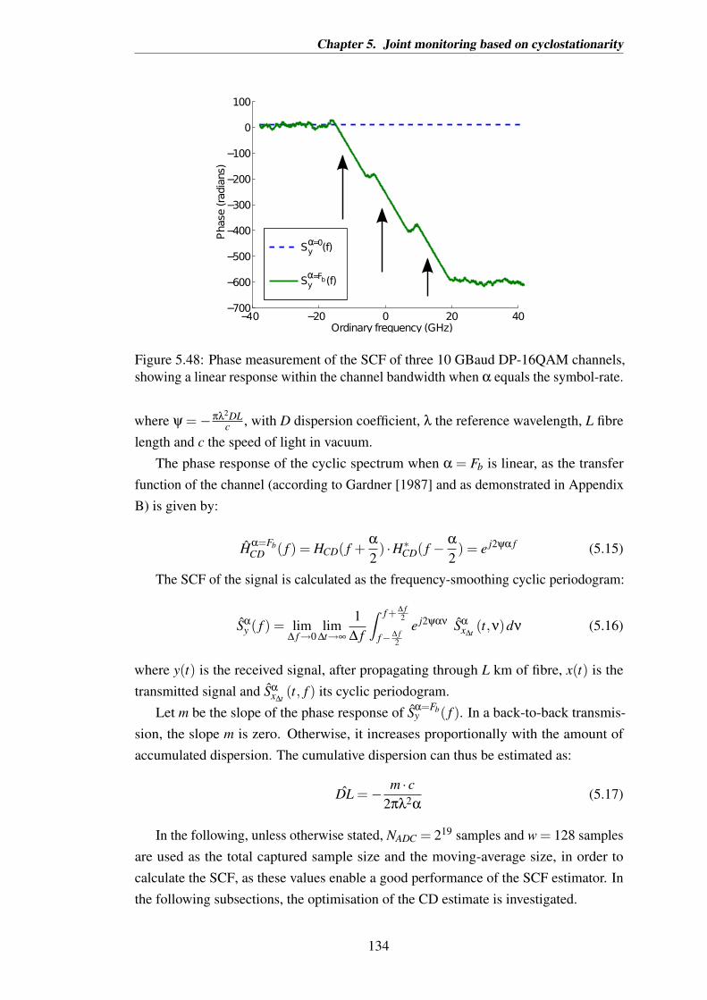
Chapter 5. Joint monitoring based on cyclostationarity
− 0 −20 0 20 40−700
−600
−500
−400
−300
−200
−100
0
100
Ordinary frequency (GHz)
Phase (ra
dia
ns)
Sy¢ =0
(f)
Sy¢ = Fb(f)α
α
Figure 5.48: Phase measurement of the SCF of three 10 GBaud DP-16QAM channels,showing a linear response within the channel bandwidth when α equals the symbol-rate.
where ψ =−πλ2DLc , with D dispersion coefficient, λ the reference wavelength, L fibre
length and c the speed of light in vacuum.The phase response of the cyclic spectrum when α = Fb is linear, as the transfer
function of the channel (according to Gardner [1987] and as demonstrated in AppendixB) is given by:
Hα=FbCD ( f ) = HCD( f +
α
2) ·H∗CD( f − α
2) = e j2ψα f (5.15)
The SCF of the signal is calculated as the frequency-smoothing cyclic periodogram:
Sαy ( f ) = lim
∆ f→0lim
∆t→∞
1∆ f
Z f + ∆ f2
f−∆ f2
e j2ψαν Sαx∆t
(t,ν)dν (5.16)
where y(t) is the received signal, after propagating through L km of fibre, x(t) is thetransmitted signal and Sα
x∆t(t, f ) its cyclic periodogram.
Let m be the slope of the phase response of Sα=Fby ( f ). In a back-to-back transmis-
sion, the slope m is zero. Otherwise, it increases proportionally with the amount ofaccumulated dispersion. The cumulative dispersion can thus be estimated as:
DL =− m · c2πλ2α
(5.17)
In the following, unless otherwise stated, NADC = 219 samples and w = 128 samplesare used as the total captured sample size and the moving-average size, in order tocalculate the SCF, as these values enable a good performance of the SCF estimator. Inthe following subsections, the optimisation of the CD estimate is investigated.
134

Chapter 5. Joint monitoring based on cyclostationarity
Impact of phase slope measurement bandwidth
0 20 40 60 80 100 1200
100
200
300
400
500
Slope measurement bandwidth (% of Channel Bandwidth)
Dis
pers
ion
RM
SE
(ps
/nm
)
roll−off = 0.07roll−off = 0.1roll−off = 0.5
Figure 5.49: Impact of the slope measurement bandwidth on the CD estimation (simula-tion of three-channel 10 GBaud DP-16QAM WDM signal).
The phase measurement is ideally centred around the channel bandwidth, andfor that reason the frequency offset information is required. However, because theproposed IF estimator presented in the previous section is coarsely accurate, the phasemeasurement is restricted over a fraction of the bandwidth of the cyclic spectrum. Thischoice enables the tolerance of higher frequency offset errors, but limits the performanceof the CD estimator at very low symbol-rates or pulse shaping bandwidths.
For a fixed transmission distance of 2421 km or fixed cumulative dispersion of40,624 ps/nm, we investigated the impact of the slope bandwidth on the CD estimation.Fig. 5.49 demonstrates that the optimum bandwidth over which the slope is measured forthe estimation of dispersion is between 60%−80% of the channel bandwidth measuredin the cyclic spectrum (which is given by the symbol-rate – roll-off product). Such asetup will impose a limit of 200 ps/nm residual dispersion RMSE for roll-offs of at least0.07. As the RRC excess bandwidth tends towards zero, the CD estimator based onthe SCF fails to perform within this error margin. For all of the following results, theestimation slope will be restricted to 70% of the cyclic spectrum bandwidth, namely:0.7 ·Fb · r.
135

Chapter 5. Joint monitoring based on cyclostationarity
Impact of frequency offset
Previously, in Section 5.5, a novel method for coarsely estimating the frequency offsetbetween the transmitter laser and local oscillator has been proposed and demonstrated.One principal motivation for it was to aid the CD estimator, by giving an approximationof the deviation from the expected frequency grid of the channel, such that the slopemeasurement can be correctly confined to the channel bandwidth.
The benefit of the proposed IF estimation on the CD estimator is evident in Fig. 5.50.If frequency offset estimation is absent, and the SCF phase slope is measured aroundDC, the CD estimation will be strongly influenced by the IF value. In particular for thelower roll-off factors, the larger frequency offsets will easily shift the channels awayfrom the 70% slope measurement bandwidth centred at DC, making it impossible forthe algorithm to measure the slope correctly. In fact, when the roll-off is 0.07, frequencyoffsets of more than approximately 25 MHz will increase the CD estimation’s RMSEabove 200 ps/nm. A coarse knowledge of the IF value is thus required, as it enables theestimation of dispersion, within the target error limit of 200 ps/nm, for IF values evenas high as 1 GHz.
It is interesting to note here that, at higher bandwidths, the IF estimation errorsincrease, but the CD estimator becomes more tolerant. This is a consequence ofrestricting the bandwidth of measurements over 70% of the channel bandwidth, whichallows more variability along the frequency axis, as induced by higher frequency offseterrors.
0 100 200 300 400 500 600 700 800 900 10000
100
200
300
400
500
Intermediate frequency (MHz)
Dis
pers
ion
RM
SE
(ps
/nm
)
roll−off = 0.07 (without IF est.)
roll−off = 0.07 (with IF est.)
roll−off = 0.1 (without IF est.)
roll−off = 0.1 (with IF est.)
roll−off = 0.5 (without IF est.)
roll−off = 0.5 (with IF est.)
Figure 5.50: Impact of frequency offset on the CD estimation (simulation of 10 GBaudWDM signals formed of three channels and modulated with DP-16QAM).
136
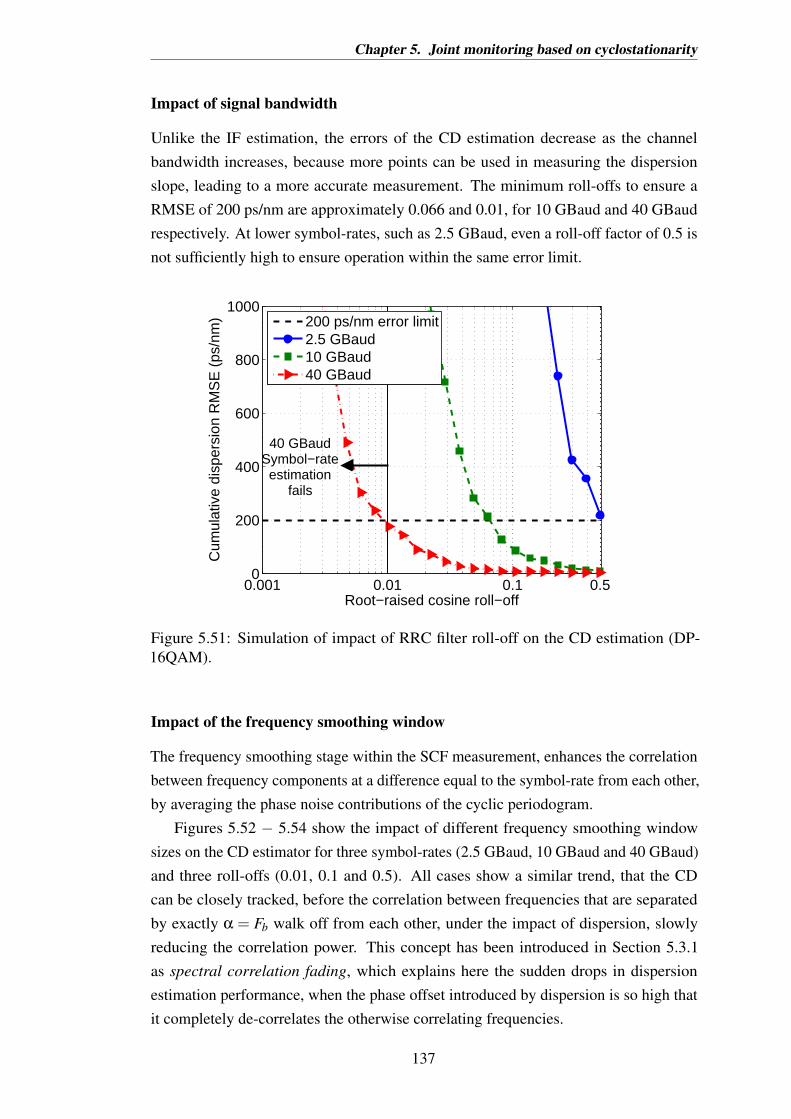
Chapter 5. Joint monitoring based on cyclostationarity
Impact of signal bandwidth
Unlike the IF estimation, the errors of the CD estimation decrease as the channelbandwidth increases, because more points can be used in measuring the dispersionslope, leading to a more accurate measurement. The minimum roll-offs to ensure aRMSE of 200 ps/nm are approximately 0.066 and 0.01, for 10 GBaud and 40 GBaudrespectively. At lower symbol-rates, such as 2.5 GBaud, even a roll-off factor of 0.5 isnot sufficiently high to ensure operation within the same error limit.
0.001 0.01 0.1 0.50
200
400
600
800
1000
Root−raised cosine roll−off
Cum
ulat
ive
disp
ersi
on R
MS
E (
ps/n
m)
40 GBaudSymbol−rateestimation
fails
200 ps/nm error limit2.5 GBaud10 GBaud40 GBaud
Figure 5.51: Simulation of impact of RRC filter roll-off on the CD estimation (DP-16QAM).
Impact of the frequency smoothing window
The frequency smoothing stage within the SCF measurement, enhances the correlationbetween frequency components at a difference equal to the symbol-rate from each other,by averaging the phase noise contributions of the cyclic periodogram.
Figures 5.52 − 5.54 show the impact of different frequency smoothing windowsizes on the CD estimator for three symbol-rates (2.5 GBaud, 10 GBaud and 40 GBaud)and three roll-offs (0.01, 0.1 and 0.5). All cases show a similar trend, that the CDcan be closely tracked, before the correlation between frequencies that are separatedby exactly α = Fb walk off from each other, under the impact of dispersion, slowlyreducing the correlation power. This concept has been introduced in Section 5.3.1as spectral correlation fading, which explains here the sudden drops in dispersionestimation performance, when the phase offset introduced by dispersion is so high thatit completely de-correlates the otherwise correlating frequencies.
137

Chapter 5. Joint monitoring based on cyclostationarity
0 5 10 15
x 105
0
5
10
15x 10
5
Cumulative dispersion (ps/nm)
Est
imat
ed c
umul
ativ
e di
sper
sion
(ps
/nm
)
w = 128w = 161w = 203w = 256w = 512
(a) 2.5 GBaud, roll-off = 0.01.
0 5 10 15
x 105
0
5
10
15x 10
5
Cumulative dispersion (ps/nm)
Est
imat
ed c
umul
ativ
e di
sper
sion
(ps
/nm
)
w = 64w = 80w = 101w = 128w = 161w = 203w = 256w = 512
(b) 2.5 GBaud, roll-off = 0.1.
0 5 10 15
x 105
0
5
10
15x 10
5
Cumulative dispersion (ps/nm)
Est
imat
ed c
umul
ativ
e di
sper
sion
(ps
/nm
)
w = 64w = 80w = 101w = 128w = 161w = 203w = 256w = 512
(c) 2.5 GBaud, roll-off = 0.5.
Figure 5.52: Impact of frequency smoothing window on the CD estimation, whensimulating three 16-QAM channels, each of 2.5 GBaud symbol-rate.
138

Chapter 5. Joint monitoring based on cyclostationarity
0 1 2 3 4 5 6 7
x 105
0
1
2
3
4
5
6
7x 10
5
Cumulative dispersion (ps/nm)
Est
imat
ed c
umul
ativ
e di
sper
sion
(ps
/nm
)
w = 64w = 128w = 161w = 203w = 256w = 512
(a) 10 GBaud, roll-off = 0.01.
0 1 2 3 4 5 6 7
x 105
0
1
2
3
4
5
6
7x 10
5
Cumulative dispersion (ps/nm)
Est
imat
ed c
umul
ativ
e di
sper
sion
(ps
/nm
)
w = 16w = 32w = 40w = 50w = 64w = 80w = 101w = 128w = 161w = 203w = 256w = 512
(b) 10 GBaud, roll-off = 0.1.
0 1 2 3 4 5 6 7
x 105
0
1
2
3
4
5
6
7x 10
5
Cumulative dispersion (ps/nm)
Est
imat
ed c
umul
ativ
e di
sper
sion
(ps
/nm
)
w = 8w = 16w = 32w = 40w = 50w = 64w = 80w = 101w = 128w = 161w = 203w = 256w = 512
(c) 10 GBaud, roll-off = 0.5.
Figure 5.53: Impact of frequency smoothing window on the CD estimation, whensimulating three 16-QAM channels, each of 10 GBaud symbol-rate.
139

Chapter 5. Joint monitoring based on cyclostationarity
0 2 4 6 8 10
x 104
0
2
4
6
8
10x 10
4
Cumulative dispersion (ps/nm)
Est
imat
ed c
umul
ativ
e di
sper
sion
(ps
/nm
)
w = 64w = 128w = 161w = 203w = 256w = 512
(a) 40 GBaud, roll-off = 0.01.
0 2 4 6 8 10
x 104
0
2
4
6
8
10x 10
4
Cumulative dispersion (ps/nm)
Est
imat
ed c
umul
ativ
e di
sper
sion
(ps
/nm
)
w = 8w = 16w = 32w = 64w = 80w = 101w = 128w = 161w = 203w = 256w = 512
(b) 40 GBaud, roll-off = 0.1.
0 2 4 6 8 10
x 104
0
2
4
6
8
10x 10
4
Cumulative dispersion (ps/nm)
Est
imat
ed c
umul
ativ
e di
sper
sion
(ps
/nm
)
w = 8w = 16w = 32w = 40w = 50w = 64w = 128w = 161w = 203w = 256w = 512
(c) 40 GBaud, roll-off = 0.5.
Figure 5.54: Impact of frequency smoothing window on the CD estimation, whensimulating three 16-QAM channels, each of 40 GBaud symbol-rate.
140

Chapter 5. Joint monitoring based on cyclostationarity
For each combination of symbol-rates and roll-offs there is an optimum rangeof window sizes that can ensure CD tracking capability with a RMSE below 200ps/nm, shown in Figure 5.55. These results have been obtained assuming knowledgeof symbol-rate and roll-off. If these two parameters are estimated within the proposedjoint estimator, the upper distance limits will be given by the interposition with those inFigure 5.24.
101
102
103
104
105
2
3
4
5
6
7
8
9
10
Maximum reach for 100% accuracy (km)
log2
(Mov
ing−
aver
age
win
dow
siz
e) (
sam
ples
)
roll−off=0.01roll−off=0.1roll−off=0.5 10 GBaud
40 GBaud
Figure 5.55: Maximum achievable distance limited by the accuracy of the CD estimation,after simulating three-channel 16-QAM WDM signals, without any linear ICI.
The number of averages must greatly exceed unity, to satisfy Grenander’s condition(Eq. 3.25) for a good spectral estimate. As the window size increases, more averagesare performed within the channel bandwidth, giving an improved slope measurement,and therefore an increased CD estimation range. However, if the moving average is toohigh, it will include more noise components than signal phase components, and thus thecyclic correlation will be lost, reducing the maximum CD value that can be correctlyestimated. This effect is more obvious for narrower channel bandwidths, for example40 GBaud signals with 0.01 roll-off and 10 GBaud signals with 0.1 roll-off. A trade-offmust be attained, for optimising the correlation of symbol phases.
If the symbol-rate and the roll-off factor are either known or estimated a priori,then the SCF can be recalculated with the optimum frequency smoothing window, suchthat the CD estimation performance is optimal, based on these results. However, fora reduced computation speed, it is preferable to use the pre-computed SCF from thesymbol-rate estimation stage. Averaging 128 samples (or equivalently, 19.53 MHz
141

Chapter 5. Joint monitoring based on cyclostationarity
for an 80 GSa/s sampling rate), is optimal in terms of the maximum reach acrossall considered combinations of symbol-rates and roll-offs, matching well with thefrequency smoothing requirements of the symbol-rate estimator.
CD estimation with 200 ps/nm is completely unreliable for the lowest consideredbandwidths, when the symbol-rate is 2.5 GBaud or the symbol-rate is 10 GBaud andthe roll-off 0.01. The cumulative dispersion estimation range increases proportionallywith the signal bandwidth, as shown in Fig. 5.55.
Estimation range
The errors increase with distance, Fig. 5.56, as a result of the fixed frequency smoothingfilter. For an increased estimation range, the filter length should decrease to adapt to thephase slope increase. However, this is not possible, as the filter size is fixed withouta priori knowledge of the distance. Alternatively, the estimation range can be furtherincreased if the error margin is relaxed. For example, for a dispersion error margin of400 ps/nm, a roll-off factor of 0.1 and 10 GBaud symbol-rate, approximately 338,620ps/nm (20,180 km) of cumulative dispersion can be estimated with this technique. Withthe same configuration, the 200 ps/nm residual dispersion target is achieved only up toa total cumulative dispersion of 162,498 ps/nm (9,684 km).
0 5000 10000 15000 20000 25000 300000
100
200
300
400
500
Distance (km)
Cum
ulat
ive
disp
ersi
on R
MS
E (
ps/n
m)
roll−off = 0.1roll−off = 0.5
Figure 5.56: Estimation range limitations of the CD estimation, for three channelsmodulated with 10 GBaud 16-QAM. The hollow marks indicate the maximum lengthup to which the symbol-rate can be estimated by simulation with 100% accuracy.
142

Chapter 5. Joint monitoring based on cyclostationarity
Independence of OSNR
The experimental investigation of Fig. 5.57 shows that AWGN does not have animpact on the CD estimator. The residual CD resulting from the estimator is less than200 ps/nm for the QPSK signal transmitted over 25 spans of fibre, compared to 140ps/nm for 16-QAM over 10 spans. The reason for the higher errors for the formercase can be accounted for by the higher CD estimation errors at longer transmissiondistances and lower roll-offs. The residual errors correspond to 14.9 km and 10.1 km ofuncompensated fibre respectively, less than 1.3% of the considered fibre lengths. Suchlow residual CD values can be compensated for by the adaptive equaliser stage whichfollows the CD static equaliser.
0 10 20 300
100
200
300
400
500
OSNR0.1nm
(dB)
Est
imat
ed d
ispe
rsio
n R
MS
E (
ps/n
m)
2017.5 km, QPSK, roll−off=0.4807 km, 16−QAM, roll−off=0.45
Figure 5.57: Experimental estimation of CD applied to a 10 GBaud homogeneousWDM signal, under different levels of noise loading.
In this section it has been demonstrated that the proposed frequency-domain CDestimation technique yields a better performance as the channel bandwidth increases,which more easily enable a correct slope measurement of the phase response. In orderto deal with RRC filtering effects and the impact of IF, the bandwidth over whichthe phase slope is measured was optimally selected as 70% of the cyclic spectrum’schannel bandwidth. NADC = 219 samples and 128 moving average taps, which give agood symbol-rate estimation as seen previously in Subsection 5.3, can also give a goodCD estimate up to 162,498 ps/nm (9,684 km of SSMF), for 10 GBaud and 0.1 roll-offfactor, limited by 200 ps/nm RMSE. With this technique, it is possible to increasethe symbol-rate whilst minimising the roll-off factor, thus allowing operation at animproved spectral efficiency. As shown here, 40 GBaud WDM channels, filtered with aRRC roll-off of 0.01, allow a CD estimation of up to 27,083 ps/nm (1614 km of SSMF),within a RMSE margin of 200 ps/nm.
143

Chapter 5. Joint monitoring based on cyclostationarity
5.6.2 Cyclic autocorrelation function approach
Subsequent to symbol-rate estimation, the CAF at the cyclic frequency equal to thesymbol-rate measures a pulse, which has a time-lag delay proportional to the amountof dispersion the signal has accumulated on its path. The pulse measured at cyclicfrequency of zero, does not experience such a shift and it therefore does not provideuseful information for the CD estimation technique. The examples in Figure 5.58 showthe two pulses without any dispersion and after the signal has travelled over 2421 km.The time domain CD estimation problem thus reduces to estimating the time delayof the cyclic autocorrelation pulse. Lowering the RRC excess bandwidth reduces thecyclic autocorrelation tone peak power as the pulse spreads. Nyquist pulse shaping is amajor limitation of this proposed CD estimation technique.
The proposed time-domain cyclostationarity approach for the estimation of disper-sion is illustrated in Fig. 5.59. The cyclic autocorrelation at α = Fb is easily extracted asonce slice of the cyclic periodogram, followed by an IFFT operation along the ordinaryfrequency. The details of this implementation can be found in Section 5.2.
The time delay is approximated as follows: the pulse peak location gives an initialcoarse delay estimate, which is dependent on the sampling rate of the receiver. Torefine this estimate, a brick wall filter is applied around the peak to limit the samplesize to 1001 samples, for an enhanced processing speed. These selected samples arethen further filtered with a moving average filter which will result in a smoothed pulse.Finally, the quadratic fit of the central 150 samples are used to obtain an improved timedelay approximation, which is then used to estimate the cumulative dispersion as:
DL =∆τ · cFb ·λ2
. (5.18)
where ∆τ is the estimated time delay, c is the speed of light in vacuum, Fb is thesymbol-rate estimate and λ is the reference wavelength. The mathematical proof of thetime-domain cyclostationarity properties under the impact of dispersion can be found inAppendix C. The number of samples used in this process have been empirically selectedwhen investigating the performance of the CD estimation technique, for the ranges ofsymbol-rates and roll-offs considered. As a result, this estimator is independent of theroll-off factor and IF, but it will be shown further that it depends on the symbol-rate.
A moving average window of approximately 64 samples is optimal for estimatingthe dispersion within the target error, but only for roll-offs higher than 0.1, as shown inFig. 5.61. As the cyclic autocorrelation pulse is lost for roll-offs of 0.01 or lower, theCD estimation cannot be performed in those instances.
Fig. 5.62 shows that the pulse time delay, as deducible from Eq. 5.18, is indeedproportional to dispersion and that it can be correctly measured by simulation, by meansof the technique just described.
144

Chapter 5. Joint monitoring based on cyclostationarity
−6 −4 −2 0 2 4 6−40
−20
0
Nor
mal
ised
CA
F (
dB)
−6 −4 −2 0 2 4 6−40
−20
0
Time−lag (ns)
α = 0
α = Fb
roll−off = 0.50 km
−6 −4 −2 0 2 4 6−40
−20
0
Nor
mal
ised
CA
F (
dB)
−6 −4 −2 0 2 4 6−40
−20
0
Time−lag (ns)
α = 0
α = Fb
roll−off = 0.52421 km
−6 −4 −2 0 2 4 6−40
−20
0
Nor
mal
ised
CA
F (
dB)
−6 −4 −2 0 2 4 6−40
−20
0
Time−lag (ns)
α = 0
α = Fb
roll−off = 0.070 km
−6 −4 −2 0 2 4 6−40
−20
0
Nor
mal
ised
CA
F (
dB)
−6 −4 −2 0 2 4 6−40
−20
0
Time−lag (ns)
α = 0
α = Fb
roll−off = 0.072421 km
−6 −4 −2 0 2 4 6−40
−20
0
Nor
mal
ised
CA
F (
dB)
−6 −4 −2 0 2 4 6−40
−20
0
Time−lag (ns)
α = 0
α = Fb
roll−off = 0.010 km
−6 −4 −2 0 2 4 6−40
−20
0
Nor
mal
ised
CA
F (
dB)
−6 −4 −2 0 2 4 6−40
−20
0
Time−lag (ns)
α = 0
α = Fb
roll−off = 0.012421 km
Figure 5.58: CD induces a time-shift in the CAF when α = Fb. 10 GBaud for all threesimulated 16-QAM channels. Correlation does not occur for a roll-off of 0.01.
delay ΔtTime
estimationCDRy(τ)
Fb
Figure 5.59: Implementation of the time-domain CD estimator.
Dependence on signal bandwidth
Fig. 5.63 shows the dependence of the estimator on the Nyquist pulse shaping bandwidth.2.5 GBaud is the lowest symbol-rate considered and can only enable CD estimationwithin the proposed error limit, if the roll-off factor is larger than 0.41. As the symbol-rate is increased, the tolerance and performance of the CD estimator with respect tothe roll-off factor improves. This is because signals of higher bandwidths have sharper
145

Chapter 5. Joint monitoring based on cyclostationarity
−600 −400 −200 0 200 400 6000
0.2
0.4
0.6
0.8
1
Time (Samples)
Nor
mal
ised
cyc
lic a
utoc
orre
latio
n
Figure 5.60: The CAF at the symbol-rate is a pulse that shifts in time with dispersion.Here, for a 10 GBaud signal and a roll-off of 0.1, a 500 km transmission is equivalentto a delay of 53.752 samples. In (blue) actual measured pulse limited to 1001 samples,(green) temporal smoothing with a moving average filter, (red) quadratic fit.
8 16 32 64 128 2560
50
100
150
200
Moving−average window (samples)
Cum
ulat
ive
disp
ersi
on R
MS
E (
ps/n
m)
roll−off = 0.1roll−off = 0.5
Figure 5.61: Simulation of the impact of the time-domain moving average filter windowon the CD estimation. Low roll-offs, such as 0.01, render the method impractical at anywindow.
pulses in the time-domain, for which the time delay can be more easily determined.Additionally, the same time-delay errors translate into smaller CD estimation errors athigher symbol-rates, as Eq. 5.18 and Figure 5.64 suggest.
At 10 GBaud, the minimum roll-off is approximately 0.069, for a RMSE of 200ps/nm. Under the same conditions, 40 GBaud signals could allow roll-offs as low as0.0178, the lowest roll-off compared to the other two considered rates, so it can beconcluded that this technique becomes more efficient as the information spectral densityof the signal increases.
146

Chapter 5. Joint monitoring based on cyclostationarity
0 5,000 10,000 15,000 20,000 25,0000
5
10
15
20
25
30
35
Distance (km)
Del
ay (
ns)
IdealMeasured
Figure 5.62: The time-domain cyclic correlation pulse experiences a time delay propor-tional to the amount of cumulative dispersion present in the signal. Simulations of 10GBaud signals, modulated with 16-QAM and filtered with a RRC of roll-off of 0.1.
0.001 0.01 0.1 0.5 10
200
400
600
800
1000
Root−raised cosine roll−off
Cum
ulat
ive
disp
ersi
on R
MS
E (
ps/n
m)
200 ps/nm limit2.5 GBaud10 GBaud40 GBaud
Figure 5.63: Impact of the RRC filter on the estimation of 40,624 ps/nm dispersion(simulations of three channels modulated with DP-16QAM).
Estimation range
As CAF pulses shift in time proportionally with the amount of dispersion accumulatedby the signal, the CD estimation range is only limited by the capture time at the receiver,provided that the symbol-rate is correctly estimated. The estimation does not exceed200 ps/nm RMSE across a wide range of fibre lengths, roll-offs as Figure 5.65 shows.The maximum cumulative dispersion values that can be correctly estimated with thistechnique ranges between 106 and 107 ps/nm, which are equivalent to over 60,000 km to600,000 km of SSMF respectively. These distances are by far exceeding the practicallyachievable distances at the respective transmission configurations.
147

Chapter 5. Joint monitoring based on cyclostationarity
0.001 0.01 0.1 0.5 10
5
10
15
20
25
Root−raised cosine roll−off
Del
ay (
ns)
Ideal2.5 GBaud (Sim.)10GBaud (Sim.)40GBaud (Sim.)
Figure 5.64: The estimation accuracy of the pulse time delay is impacted by the roll-offfactor. The amount of cumulative dispersion is fixed to 40,624 ps/nm (2421 km ofSSMF), but the time delay changes with the symbol-rate.
103
104
105
106
107
1080
100
200
300
400
500
Cumulative dispersion (ps/nm)
Dis
pers
ion
RM
SE
(ps
/nm
)
roll−off = 0.018roll−off = 0.1roll−off = 0.5
(a) 2 GBaud, 3 channels 16-QAM.
103
104
105
106
107
1080
100
200
300
400
500
Cumulative dispersion (ps/nm)
Dis
pers
ion
RM
SE
(ps
/nm
)
roll−off = 0.018roll−off = 0.1roll−off = 0.5
(b) 10 GBaud, 3 channels 16-QAM.
103
104
105
106
107
1080
100
200
300
400
500
Cumulative dispersion (ps/nm)
Dis
pers
ion
RM
SE
(ps
/nm
)
roll−off = 0.018roll−off = 0.1roll−off = 0.5
(c) 40 GBaud, 3 channels 16-QAM.
Figure 5.65: Estimation of CD by means of CAF, applied to homogeneous WDMsignals traversing different lengths of SSMF fibre, by simulation.
148

Chapter 5. Joint monitoring based on cyclostationarity
Figure 5.66 shows that the technique works experimentally for 16-QAM and QPSKmodulation formats, independent of the OSNR value at the receiver. The errors are notexceeding 200 ps/nm when transmitting over 2018 km of fibre and 807 km (QPSK and16-QAM respectively), but these could in essence be compensated for by the dynamicequaliser.
0 10 20 300
100
200
300
400
500
OSNR0.1nm
(dB)
Est
imat
ed d
ispe
rsio
n R
MS
E (
ps/n
m)
2017.5 km, QPSK, roll−off=0.4807 km, 16−QAM, roll−off=0.45
Figure 5.66: Experimental estimation of CD applied to a 10 GBaud homogeneousWDM signal, under different levels of noise loading.
5.6.3 Comparison between the time domain and frequency domainchromatic dispersion estimators
This section demonstrated by simulation and experimentally the feasibility of time andfrequency domain CD estimators, based on the cyclostationarity properties of modulatedsignals. Although based on the same statistical properties, the differing implementationapproaches between the two functions result in performance differences in terms ofdispersion estimation range or bandwidth requirements.
The SCF is computed as the frequency averaged cyclic periodogram, whilst the CAFis the IFFT of the cyclic periodogram. Frequency averaging performed with a movingaverage filter introduces correlation fading and therefore a decrease in performancewith an increase in dispersion. Unlike the CD estimator based on the SCF, the CAFimplementation can allow under 200 ps/nm RMSE up to 2,098,926 ps/nm cumulativedispersion (equivalent to 125,085 km of SSMF) when the symbol-rate is 40 GBaud andthe roll-off factor is 0.018, This is a consequence of the robustness of the CAF, which ispractically CD independent as Section 5.3.2 demonstrated. The maximum cumulativedispersion that can be estimated with either technique varies with signal bandwidth, as
149

Chapter 5. Joint monitoring based on cyclostationarity
listed in Table 5.8.The preceding symbol-rate, roll-off and frequency offset estimates are needed for
this CD estimation stage, when the SCF is used. The CAF approach requires onlyknowledge of the symbol-rate.
The two techniques show a similar behaviour with respect to channel bandwidth,both requiring larger bandwidths for an increased estimation accuracy, as summarisedin Table 5.9. The SCF performs slightly better as the symbol-rate increases, allowingslightly lower roll-off values.
Computationally, the two approaches are very similar, as the dominating complexitycomes from the correlation functions, which both require NADC log2 NADC complexmultiplications. Both techniques are independent of impairments such as AWGN,transmitter and LO phase offset and phase noise.
It can be concluded that the frequency-domain implementation of the CD estimator ispreferable, as its performance improves with respect to pulse shaping excess bandwidthlimitations, as the symbol-rate increases.
Spectral Correlation FunctionSymbol-rate Maximum achievable range (ps/nm)
(GBaud) roll-off = 0.01 roll-off = 0.1 roll-off = 0.52.5 – – –10 – 1,313,522 1,027,79740 27,083 185,518 219,372
Cyclic Autocorrelation FunctionSymbol-rate Maximum achievable range (ps/nm)
(GBaud) roll-off = 0.0178 roll-off = 0.1 roll-off = 0.52.5 – – 1,614,00010 – 16,249,752 35,207,79640 2,098,926 8,531,120 9,343,607
Table 5.8: Maximum achievable cumulative dispersion estimation with RMSE under200 ps/nm, for the two proposed chromatic dispersion estimators, based on the SpectralCorrelation and on the Cyclic Autocorrelation Functions.
Symbol-rate Minimum allowable RRC roll-offSCF-CDE CAF-CDE
2.5 GBaud >0.5 0.412110 GBaud 0.066 0.069240 GBaud 0.0092 0.0178
Table 5.9: Bandwidth requirements for the two proposed chromatic dispersion estima-tors, based on the Spectral Correlation and on the Cyclic Autocorrelation Functions.
150

Chapter 5. Joint monitoring based on cyclostationarity
5.7 In-band OSNR estimation
Using the different statistical properties of linearly modulated signals, which are wide-sense cyclostationary, and AWGN, which is wide-sense stationary, it is possible toestimate the in-band OSNR, as demonstrated herein.
−20 −10 0 10 20−160
−155
−150
−145
−140
−135
−130
−125
−120
−115
−110
Frequency (GHz)
Po
we
r/fr
eq
ue
ncy (
dB
/Hz)
Sx
0, OSNR = 14.2 dB
Sx
10.7GHz, OSNR = 14.2 dB
(a) roll-off of 1
−20 −10 0 10 20−160
−155
−150
−145
−140
−135
−130
−125
−120
−115
−110
Frequency (GHz)
Po
we
r/fr
eq
ue
ncy (
dB
/Hz)
Sx
0, OSNR = 14.2 dB
Sx
10.7GHz, OSNR = 14.2 dB
(b) roll-off of 0.25
Figure 5.67: Spectral Correlation Functions calculated for three simulated WDMchannels, modulated at 10GBaud with DP-16QAM and Nyquist pulse-shaping. Thearrows delimit the bandwidths over which the powers are integrated.
As Fig. 5.67 shows, when α = 0 the SCF is the traditional power spectral densityof the signal with additive noise. Conversely, the cyclic spectral density when α = Fb
measures the signal power only, since AWGN is not a cyclostationary process andit will not correlate at this cyclic frequency. The OSNR can thus be estimated fromthe two SCFs: Sα=0
x ( f ) and Sα=Fbx ( f ). In a noise-free measurement, the two cyclic
spectra will differ by a scaling factor k, which needs to be pre-calculated as part of acalibration stage. When the signal is noise-loaded, the average powers Pα=0
ave and Pα=Fbave
are calculated over fixed bandwidths, corresponding to both SCFs.Assuming a fixed signal launch power, but varying optical paths and therefore
varying accumulated noise levels, Pα=0ave decreases with OSNR, whilst Pα=Fb
ave is approx-imately constant over the entire OSNR interval. At lower OSNRs, there is howevera slight increase in Pα=Fb
ave with noise. This is due to the fact that both Sα=0x ( f ) and
Sα=Fbx ( f ) scale with noise power, in the same proportion that the autocorrelation of
noise scales with noise power. When the OSNR is very low, below 5 dB, the high noisepower becomes a significant term in Sα=Fb
x ( f ).These power measurements finally lead to the OSNR estimate:
OSNR = 10log10
(kPα=Fb
ave
kPα=0ave − kPα=Fb
ave
Bres
Bre f
). (5.19)
Bres and Bre f are the resolution and reference bandwidths respectively.
151

Chapter 5. Joint monitoring based on cyclostationarity
0 5 10 15 20 25−3
−2.5
−2
−1.5
−1
−0.5
0
0.5
OSNR0.1nm
(dB)
Mea
sure
d av
erag
e po
wer
(dB
m)
Paveα=0
k⋅Paveα=F
b
Figure 5.68: SCF power measurements at cyclic frequencies of 0 and symbol-rate.
A correct estimation of the OSNR is thus directly dependent on a correct estimationof the two average powers Pα=0
ave and Pα=Fbave . In order to improve the estimate, the OSNR
is averaged between the two polarizations. A schematic of the digital implementationof this technique is depicted in Fig. 5.69. After CD compensation, which is required toavoid power fading, the SCF is recalculated for only two cyclic-frequencies, at 0 and atthe estimated symbol-rate.
xCDcomp(t)
2| | Sx(f)0F
SNSCF
∫ ( ) dfΔf/2
-Δf/2
∫ ( ) dfFb/2
-Fb/2
PFb
P0
OSNR
NSCF
*Sx(f)
ejπFbt
e-jπFbtNFFT
FFT
FFT
NFFT
FS
F
FFT
NFFT
b
Figure 5.69: Single polarisation implementation of the SCF-based OSNR estimation.
In the two examples of Fig. 5.67, three 10 GBaud 16-QAM WDM channels arespaced at 12.5 GHz and are Nyquist pulse-shaped with a RRC filter of roll-off of 0.25and 1 respectively. When ICI is present, as in this case, the powers are measured overrestricted bandwidths, less than the entire bandwidth of the channel of interest, in orderto avoid power measurements of the adjacent channels, which would in turn result inan overestimation of the signal power. At higher symbol-rates, if the bandwidth of thechannel would exceed the receiver bandwidth, then the powers would be integrated overthe entire receiver bandwidth. The average powers Pα=0
ave and Pα=Fbave were measured over
Fb and Fbroll−o f f
2 bandwidths respectively. Finally, the OSNR was estimated accordingto Eq. (5.19), with a 10 GHz resolution bandwidth and 0.1 nm reference bandwidth.
152

Chapter 5. Joint monitoring based on cyclostationarity
5.7.1 Back-to-back Transmission
Figures 5.70 and 5.71 show the range over which the OSNR can be estimated withinthe acceptable error margin, for a fixed RRC roll-off, in a back-to-back setup. Athigher OSNRs, low noise powers are more difficult to estimate, resulting in a limitedestimation accuracy for higher OSNRs. A correct estimation is achieved up to 12 dBOSNR for DP-QPSK and up to 16 dB OSNR for DP-16QAM. Since the ROSNR is7.6 dB for 10 GBaud DP-QPSK and 14.2 dB for 10 GBaud DP-16QAM, the range ofcorrect estimation includes the ROSNR by a margin.
4 6 8 10 12 14 162
4
6
8
10
12
14
16
18
OSNR0.1nm
(dB)
Est
imat
ed O
SN
R0.
1nm
(dB
)
SimulationExperiment
ROSNR for BER = 3.8x10 −3
Figure 5.70: OSNR estimation for DP-QPSK in a back-to-back setup and a RRC roll-offof 0.4.
Since 16-QAM operates at higher OSNRs, the receiver’s noise starts to becomelimiting from around 19 dB OSNR. The calibration of noise-free estimation is moresensitive for 16-QAM compared to QPSK, and in estimating the same OSNR, the errorswill be higher than in the case of QPSK, despite the fact that the method is independentof modulation format. In both cases, there is a good agreement between simulationand experimental results. Additionally, the probability density function of the OSNRestimation errors is not necessarily a symmetric Gaussian distribution, but it can beskewed, as Fig. 5.72 shows for example. The upper bound on the OSNR estimationrange highly depends on the number of samples processed, the roll-off factor and CD,which are treated next.
Fig. 5.73 shows the dependency of the estimation on the number of samples, basedon experimental results, for a fixed symbol-rate of 10 GBaud and its corresponding
153

Chapter 5. Joint monitoring based on cyclostationarity
8 10 12 14 16 18 20 22 24 265
10
15
20
25
30
OSNR0.1nm
(dB)
Est
imat
ed O
SN
R0.
1nm
(dB
)
SimulationExperiment
ROSNR for BER = 3.8x10 −3
Figure 5.71: OSNR estimation for DP-16QAM in a back-to-back setup and a RRCroll-off of 0.45.
−5 0 50
20
40
60
80
100
120
140
OSNR estimation error (dB)
Pro
babi
lity
dens
ity fu
nctio
n
σ+
σ−
Figure 5.72: Estimation of the ROSNR for DP-16QAM in a back-to-back experimentalsetup and a RRC roll-off of 0.45.
154

Chapter 5. Joint monitoring based on cyclostationarity
2 4 6 8 10 12 140
1
2
3
4
5
6
log2(Moving−average window size) (taps)
Max
imum
OS
NR
0.1n
m e
stim
atio
n er
ror
(dB
)
NADC
= 217
NADC
= 218
NADC
= 219
Error limit
Figure 5.73: Impact of frequency smoothing window on the in-band OSNR estimation,for a three channel DP-16QAM WDM in a back-to-back simulated transmission.
ROSNR, to ensure a BER of 3.8 ·10−3. The accuracy increases with a higher number ofsamples captured by the ADC, because that is equivalent to an increase in the numberof points over which the STFT is computed, leading to a better SCF estimate. At least218 samples are required for correct power estimations that would result in errors lessthan 1.5 dB, as required by ITU [2012] standard.
The spectral smoothing window is also essential in optimizing the estimation. Whenthe window size is too low, the absolute errors increase as the number of spectralaverages is not sufficient in obtaining an accurate approximation of the SCF in Eq.3.23. On the other hand, when the window size is high and close in value to NADC, theerrors increase as a result of the reduced resolution of the SCF. The optimum averagingwindow size when NADC = 218 samples is between 128−512 samples.
The RRC roll-off is a limiting factor for the in-band OSNR estimation as shown inFig. 5.74. At lower roll-offs the signal bandwidth is reduced, as depicted in Fig. 5.67,for both α = 0 and α = Fb. Because the power integration bandwidth is even lower whenα = Fb, the measurement accuracy of Pα=Fb
ave will be reduced under the low roll-offsconditions and thus leading to higher OSNR estimation errors. The performance hereis evaluated in terms of the standard deviation of the measured error, across all 100estimations. Roll-offs higher than 0.1 induce higher errors also in the measurement ofthe IF, which the OSNR estimator relies on.
Increasing the order of the modulation format, will result in more stringent lim-itations of the presented technique in terms of achievable roll-offs. For DP-QPSK,
155

Chapter 5. Joint monitoring based on cyclostationarity
0.001 0.0032 0.01 0.032 0.1 0.32 10
1
2
3
4
5
6
7
8
9
10
Root−raised−cosine filter roll−off
Err
or s
tand
ard
devi
atio
n (d
B)
QPSK (Sim)16−QAM (Sim) QPSK (Exp)16−QAM (Exp) Error limit
Roll−off=0.0578891.74 bits/s/Hz/pol
ROSNR=7.6dB
Roll−off=0.301063.2 bits/s/Hz/polROSNR=14.2dB
Figure 5.74: Impact of RRC roll-off factor on the in-band OSNR estimation, for a threechannel WDM signal in a back-to-back transmission.
the minimum roll-off of 0.06 gives the maximum acceptable error of 1.5 dB, whilefor DP-16QAM this value is 0.3. The difference in the roll-off tolerance for the twomodulation formats comes from their different ROSNRs. Depending on the modulationformat used, the roll-off limitation also imposes constraints on the maximum achiev-able spectral efficiency. Although the requirements on the maximum roll-off are morestringent for 16-QAM compared to QPSK, the achievable spectral efficiency is stillincreased almost two-fold when using 16-QAM modulation format. Again, there is agood match between simulation and experimental results.
5.7.2 Standard Single Mode Fiber Transmission
Fig. 5.75 and 5.76 show that the OSNR estimation can be performed over distances of2017.5 km for DP-QPSK and 807 km in the case of DP-16QAM. The power fluctuationsin the experimental setup, due to the instability of the Acusto-Optic Switch (AOS) andPDL, which cause fluctuations in the OSNR measurement. However, the errors are stillwithin the 1.5 dB imposed error margin, at the ROSNR. The receiver noise starts todominate at around 19 dB OSNR, and it is the only source of error at high OSNRs.
156

Chapter 5. Joint monitoring based on cyclostationarity
5 10 15 20 250
5
10
15
20
25
30
35
OSNR0.1nm
(dB)
Est
imat
ed O
SN
R0.
1nm
(dB
)
SimulationExperiment
ROSNR for BER = 3.8x10⁻³
Figure 5.75: OSNR estimation for DP-QPSK and a transmission distance of 2017.5 kmand a RRC roll-off of 0.4.
10 15 20 25 30 355
10
15
20
25
30
35
40
OSNR0.1nm
(dB)
Est
imat
ed O
SN
R0.
1nm
(dB
)
SimulationExperiment
ROSNR for BER = 3.8x10⁻³
Figure 5.76: OSNR estimation for DP-16QAM and a transmission distance of 807 kmand a RRC roll-off of 0.45.
157

Chapter 5. Joint monitoring based on cyclostationarity
5.8 Conclusions
This chapter demonstrated novel joint estimation techniques, based on the cyclosta-tionarity properties of linearly modulated signals, that can efficiently be implementedwithin the digital coherent receiver DSP for monitoring purposes in SDONs. The stagesof the joint monitor consist of symbol-rate, roll-off IF, CD and OSNR estimations,consecutively applied in this order.
A correct symbol-rate estimation is essential for the reliability of the entire jointestimator. The conditions under which the symbol-rate estimation can perform with100% accuracy have been investigated in detail, including the impact of acquisitiontime, symbol-rate range, pulse shaping, as well as chromatic dispersion and noise. Time-domain and frequency-domain implementations have been discussed and compared interms of their performance.
The frequency-domain implementation, based on the SCF, employs a frequency-smoothing filter for enhancing the spectral correlation through noise averaging. Themain limitation of this technique is its dependence on CD, which results in correlationfading as demonstrated for the first time in this chapter. The optimum frequency-smoothing window changes with distance and signal bandwidth, but in order to cover awide range of possible required capacity – spectral-efficiency – reach combinations, awindow size of 128 – 256 samples is sufficient for a reliable symbol-rate estimation.Although limited by dispersion, the method allows the accurate estimation of 40 GBaudup to 1,614 km at a roll-off of 0.01 or 3,228 km at a roll-off of 0.1. On the other hand,the time-domain implementation, based on the CAF, does not employ a moving-averagefilter and is as a result almost completely independent of CD. The main limitation ofboth the time-domain and frequency-domain approaches is that they cannot performwell when the excess bandwidth of the Nyquist pulse shaping filter tends to zero. Whenthe symbol-rate is 10 GBaud, the SCF-based estimator allows a 1% minimum roll-off,whilst the CAF approach requires at least 7% excess bandwidth. The frequency domainapproach is thus preferred for symbol-rate estimation.
The CAF is more sensitive to the RRC roll-off and can therefore be used to estimateit, from the power ratio between the CAF tone at the cyclic frequency equal to thesymbol-rate and its DC component. Roll-off factors down to 0.06 can be estimatedwithin a RMSE of < 20%, independently of IF, noise or CD.
From the spectral correlation at the symbol-rate estimate, a new IF estimationtechnique has been demonstrated. Contrary to the CD estimation stage that succeeds it,a lower roll-off factor is of benefit to the IF estimation. For three channels at 10 GBaud,the RMSE is 14 MHz for a roll-off of 0.5 and 4 MHz for a roll-off of 0.1, sufficient forthe following CD and OSNR estimation stages.
Time-domain and frequency-domain cyclostationarity-based CD estimation tech-
158

Chapter 5. Joint monitoring based on cyclostationarity
niques have been proposed and demonstrated here for the first time. The formermeasures the time delay of the CAF pulse, while the latter measures the phase of thecyclic spectrum within the channel bandwidth, both giving an estimate of the amountof cumulative dispersion in the signal. A sufficiently low RMSE limit of 200 ps/nmresidual uncompensated CD is imposed, as it can be corrected for by the dynamicequaliser at the very low cost of employing 2 extra taps at 10 GBaud. For a more reli-able performance, both techniques require high channel bandwidths, achievable eitherby increasing the symbol-rate or the roll-off factor. At 40 GBaud, the time-domainimplementation functions for roll-offs as low as 0.018, whilst the frequency-domainmethod can achieve the same performance for a minimum roll-off of 0.01. In terms ofspectral efficiency this means an 8% improvement, which becomes siginificant whenmoving to data-rates of 400 Gb/s and beyond. The SCF-based approach is thus pre-ferred, as it improves the CD estimation with respect to roll-off limitations, with anincrease in the symbol-rate. However, if a longer transmission distance is desirable,then the time-domain implementation enables the estimation of up to 2,098,926 ps/nm,at a RMSE of 200 ps/nm, outperforming the frequency-domain approach. For a fasterprocessing speed, the CAF-based CD estimator can be applied simultaneously with theIF and the roll-off estimators, as it is independent from them.
The in-band OSNR can be estimated by using the cyclostationarity property oflinearly modulated signals, with certain constraints. This method is particularly usefulfor Nyquist WDM systems, when the roll-off factor is larger than 0.06 for DP-QPSKand 0.3 for DP-16QAM, but results in errors higher than 1.5 dB otherwise, even when219 samples are processed. The accuracy can be improved by capturing more samples atthe receiver, at the cost of a longer estimation time, and from a correct selection of thespectral smoothing window size. The ROSNR of 10 GBaud DP-QPSK and DP-16QAMfor BER of 3.8 ·10−3 falls within the range of OSNRs that can be correctly estimatedwithin 1.5 dB of error. The method requires knowledge of the symbol-rate, RRC roll-offfactor and CD, but as demonstrated these parameters can be also estimated using thesame cyclostationarity approach.
To enhance the cyclic correlation features of the signal, 219 samples are processedwhich requires an acquisition time of 6.55 µs when the sampling rate is 80 GSa/s. Incurrent dynamic optical networks reconfiguration and the DSP data recovery algorithmoperate on a µs time-scale, which makes the proposed joint estimator suitable for practi-cal implementation. For a faster processing time, a compromise between transmissioncapacity-distance product and accuracy is needed. Finally, the linear or non-linear noisecomponents have no impact on the joint estimator.
159

6Conclusions and future work
As the evolution of electronics speed seems to have reached a halt, capacity increasesin future optical networks will no longer be able to meet traffic demands, by simplyincreasing the symbol-rate. Increasing the modulation format order limits the trans-mission distance, and this approach also fails when aiming to increase the channelcapacity. Moreover, legacy systems are inherently over-engineered, as they supportonly static signal configurations. In response to this capacity crunch, optical networksare becoming more software-defined in order to optimise spectral utilisation, and de-fine transmission parameters according to existing demands and channel impairments.For instance, data-rates exceeding 1 Tb/s can be achieved by employing flexible gridNyquist WDM superchannels, which enable flexibility in the spectral domain, as wellas capacity and reach to be customised to specific application requirements. Whilstoptical networks become more dynamic and reconfigurable, they require monitoringfor maintenance purposes. In addition, SDON could reach autonomy, required foroptimised reconfigurability, through persistent and continuous self-observation. It isthus equally important to enable sensing of both future superchannels, but also legacychannels operating at lower symbol-rates and OOK or BPSK formats.
The introduction of coherent detection with DSP enabled programmable receivers,capable of adaptively monitoring and compensating fibre impairments. As such, sens-ing integrated within the digital domain of coherent receivers is currently the mostcost-effective solution, given the increased sampling speed of existing ADCs andComplementary Metal-Oxide-Semiconductor (CMOS) scalability, together with the
160

Chapter 6. Conclusions and future work
employment of digital coherent receivers on a large scale. Future digital monitoringtechniques require to be as independent as possible of the data-recovery algorithms,such that monitoring can be performed at the beginning stages of the DSP, for increasedfeedback response towards the control plane.
The most common parameters that would change dynamically are: symbol-rate,FEC, roll-off, modulation format, reach, OSNR and wavelength. In particular, thereach depends on transmitted power, symbol-rate, superchannel configuration andexisting fibre impairments. The following sections explain how this work meets theaforementioned goals and how it compares with monitoring techniques existing inliterature, which have already been presented and discussed in Chapter 2.
6.1 Research summary
The work that forms the body of this thesis focused on the estimation of symbol-rate,CD, and OSNR, which are some of the main parameters to be employed in decision-making regarding transmission reconfiguration. The roll-off factor of the transmitterRRC pulse shaping filter and the IF between the transmitter and LO lasers have alsobeen estimated, as enablers to the proposed CD and OSNR techniques. All techniquespresented here have been demonstrated for M-PSK and M-QAM modulation formats,but are also applicable to OOK.
Symbol-rate estimation
Three different signal-transforming symbol-rate estimation techniques have been demon-strated, all based on spectral properties of modulated signals. Chapter 3 provides thebasic theory required for the understanding of these techniques.
A novel symbol-rate estimator, based on measuring the spectral variance, that workswell at Nyquist pulse shaping of zero excess bandwidth, is demonstrated in Chapter 4.The extent of its independence of IF, dispersion and AWGN has been demonstrated. Theabsolute error is of the order of MHz, which may be slightly high for timing recoveryalgorithms that require an accuracy of the order of kHz. However, the accuracy issufficient to distinguish between different FEC levels, from a known set of values. Themain drawback of this algorithm is that it would not function for WDM systems, as itsperformance depends on the measurement of the individual channel bandwidth. Thistechnique is therefore applicable only to single-channel legacy systems.
In Chapter 5, two different approaches for estimating the symbol-rate are addi-tionally investigated, based on the time-domain and frequency-domain properties ofcyclostationarity signals, by measuring their CAF and SCF respectively. Whilst the twofunctions are Fourier pairs, their implementation differed by additionally employing
161

Chapter 6. Conclusions and future work
a moving-average filter to reduce the spectral variance for the SCF approach. Thus,their complexities are comparable, but their performances slightly different. The maindifference brought by the inclusion of the frequency domain smoothing filter, is thatit limits the transmission distance achievable with this technique due to spectral cor-relation fading. On the other hand, in the absence of this filter the CAF symbol-rateestimator is virtually CD independent.
Both are limited by Nyquist pulse shaping of reduced excess bandwidths, whichreduces the cyclic correlation. The CAF approach has been previously proposed inliterature, but a significant improvement has been brought to it herein by employing afiner spectral resolution. Whilst a RRC roll-off of only 0.2 was permitted in previousresults, here it is possible to go to roll-offs as low as 0.07, enabling Nyquist superchanneloperation. Nonetheless, the novel SCF approach, proposed here for the first time, ispreferred, as it allows roll-offs as low as 0.01.
In the literature, it is found that the reconfiguration time of coherent transceiversis less than 150 ns and the time required for the DSP to recover the data is less than200 ns. The single-channel symbol-rate estimator requires a comparable amount oftime, 655 ns, for collecting sufficient data for the estimation. On the other hand thecyclostationarity-based symbol-rate estimators are limited by a 6.55 µs digitisation time.This latter value is still acceptable, as the amount of time to transfer the informationover 1000 km of SSMF, if data-aided estimation was employed instead, is 10 ms.
Whilst three orders of magnitude slower than the single-channel technique, thepossibilities of the cyclostationarity estimation are greater by comparison. The accuracyis much higher, of the order of kHz, it enables estimation across the entire WDM signalwithout need for demultiplexing, and the estimation of other parameters is enabledsubsequently, from the same technique.
Roll-off estimation
The estimation of the roll-off factor is a rare subject in the literature and it is brieflytouched upon in this thesis. The applicability of such an estimator lies both in theupdate of the match-filter at the receiver, but also of the subsequent CD and OSNRestimators investigated in this work. Based on the time-domain CAF, the proposedroll-off estimator performs within RMSE of 20% for roll-offs between 0.06 and 0.3,which is an acceptable performance [Yang et al., 2009].
Frequency offset estimation
A spectrum-based IF estimator was also demonstrated here, in order to aid the CD andOSNR estimators, by centering their measurements around the channel location. Thereis a good correspondence between this estimator and the estimator based on the fourth
162

Chapter 6. Conclusions and future work
power measurement, followed by an iterative spectral search of the carrier, typicallyemployed in the coherent receiver’s DSP. The RMSE of 4 MHz has been demonstratedfor a roll-off of 0.1, and this value improves as the roll-off factor decreases.
Chromatic dispersion estimation
Two novel algorithms are proposed for the estimation of CD, based on the same SCFand CAF functions. Similarly to the symbol-rate estimation, the frequency domainapproach is limited by correlation fading. By contrast, the CAF allows the estimationof 2,098,926 ps/nm cumulative dispersion (equivalent to 125,085 km of SSMF) whenthe symbol-rate is 40 GBaud and the roll-off factor is 0.018. This by far exceeds theperformance of the existing CD estimators implemented within the coherent receiverand requires only Nlog2N computations, where N is the total number of samples. Themain limitation of this technique is the narrow pulse shaping performed at the receiver.The SCF-based approach is thus preferred as it improves the CD estimation down toroll-offs as low as 0.01, giving a 8% improvement in terms of spectral efficiency, whichbecomes siginificant when moving to data-rates of 400 Gb/s and beyond. The targetresidual dispersion error proposed here was a RMSE of 200 ps/nm, which is sufficientlylow to limit the number of taps of the dynamic equaliser, required to compensated for it.
Optical signal-to-noise ratio estimation
In recent years, there has been an increased focus on in-band OSNR monitors thatcould be integrated within the coherent receiver DSP, motivated by their wide employ-ment with high data-rate systems, which means that these monitors could be cheaplyincorporated into their design. The ITU-T recommendation is of 1.5 dB maximumallowable OSNR estimation error. It is desirable to implement OSNR estimation that isindependent of other DSP steps.
A previously proposed OSNR estimator based on cyclostationarity properties ofsignals, has been further investigated in this thesis. It was confirmed both by simulationand experimentally the the performance of this estimator is within the 1.5 dB errorlimit, and in addition, does not require PMD compensation, nor symbol recovery. It ishowever dependent on CD, and requires approximate knowledge of the channel locationand bandwidth, which have all been made possible with the previously presentedestimators. The OSNR estimation algorithm also requires a calibration stage, which canbe appropriate for burst-mode switching networks where a period of receiver training isalready employed.
163

Chapter 6. Conclusions and future work
Joint parameter estimation
Jointly monitoring of any of the required parameters is a faster and more computationallyefficient solution. In the literature, the majority of the joint estimation techniques focuseither on the transmission parameters or the channel parameters. In this thesis, jointestimation of both classes has been demonstrated, which is of particular significance,when the changing of the signal configuration and transmission path at the transceivernodes are both inter-dependent.
Compared to the joint estimator based on the FIR filter coefficients [Hauske et al.,2008], the cyclostationarity technique can be executed in approximatelly the sameamount of time (of the order of µs). In the absence of DGD, both OSNR estimatorsperform similarly with maximum 1 dB and 1.5 dB absolute errors for the FIR filtertaps and cyclostationarity approaches respectively. In this work, a RMSE of 200 ps/nmwas self-imposed for the CD estimation performance, which allows an esimation rangeup to 27,083 ps/nm when the roll-off is 0.01 and the symbol-rate is 40 GBaud. Theequaliser approach on the other hand allows a more precise CD estimation of 63 ps/nmstandard deviation, but was only tested for up to 2000 ps/nm. Furthermore, the FIRfilter technique requires demultiplexing and timing recovery, and it has not been testedfor Nyquist pulse shaped signals.
As Nyquist WDM superchannels are becoming ubiquitous, joint performance moni-tors will need to focus more on signals that have undergone pulse-shaping approachingthe Nyquist limit, since not so many have been given consideration in the literature sofar. In this thesis such a joint estimator has been demonstrated. Its operation is limitedby the narrowest pulse shaping, when the RRC roll-off is less than 0.3, and could alsobenefit of higher ADCs and processors speeds. Since it has a high potential, more workis required to further investigate and improve this joint estimator, as proposed in whatfollows.
6.2 Proposed future work
Further work could be performed in investigating the potential of the proposedcyclostationarity-based joint estimator. Whilst the work in this thesis demonstratedthe applicability of the frequency offset, CD and OSNR estimators only for the centralchannel, the same approach can also be applied to the individual subchannels of theentire superchannel. Moreover, the linear CD phase response of the SCF computedat the symbol-rate, for channels that have travelled on different optical paths, couldbe estimated individually, from a single computational effort. Such signals are notsuperchannels by definition, but they are a common occurrence in networks employingROADMs, where channels are added and dropped at different nodes within the network,
164

Chapter 6. Conclusions and future work
and therefore also need consideration.As demonstrated in this thesis, symbol-rate estimation can be performed on hetero-
geneous WDM superchannels, where tones linking to each unique symbol-rate can bedetected. However, the correspondence between the channel rate and channel locationis lost, and this information could be recovered through further DSP techniques. Oneproposed approach is to perform spectral scanning, and use the already estimated pa-rameters in doing so. Subsequent to symbol-rate and roll-off estimation, the analyticalspectrum can be generated on a per-channel basis. From the frequency offset estimator,the location of existing channels can be identified. Further, it may then be possible tocorrelate the spectrum of the superchannel with the analytical spectrum of the channelto be searched for, and finally identify which channel corresponds to which bandwidth.
More work needs to be done to reduce the number of samples required in thecomputation of the SCF, and thus improve the response time of the estimate to similartime-scale as the network elements switching time (ns order). Using weighing windowsother than rectangular windows, as assumed throughout this thesis, usually decreasesspectral leakage of the conventional PSD. However, when computing the SCF, spectralleakage increases the spectral correlation and it is desirable. It is thus expected thatapodisation limits the cyclostationarity of modulated signals, and more tests are requiredto confirm this.
One possible alternative approach to the Welch’s method, that has been left unex-plored so far, is to employ the Multi-taper method for computing the SCF. Whilst bothmethods aim at reducing the variance of the periodogram, the Multi-taper approachcan give a better trade-off between low variance and high resolution, and thus has thepotential to operate with a lower number of samples.
Finally, better pulse delay estimators need to be investigated, as having the potentialto improve the time-domain CD estimator even further.
165

References
S. Abbott, “Review of 20 years of undersea optical fiber transmission system develop-ment and deployment since TAT-8,” in Optical Communication, 2008. ECOC 2008.34th European Conference on, 2008, pp. 1–4. 12
T. Anderson, A. Kowalczyk, K. Clarke, S. Dods, D. Hewitt, and J. Li, “Multi impairmentmonitoring for optical networks,” Lightwave Technology, Journal of, vol. 27, no. 16,pp. 3729–3736, Aug 2009. 38, 39
L. Baker-Meflah, B. Thomsen, J. Mitchell, and P. Bayvel, “Multi-impairment WDMoptical performance monitoring for burst switched networks,” Lightwave Technology,Journal of, vol. 28, no. 23, pp. 3417–3426, Dec 2010. 38, 39
W. Barnes, N. LaSorte, H. Refai, and M. Yeary, “Symbol rate classification ofPSK/QAM signals using direct frequency estimators,” in Instrumentation and Mea-surement Technology Conference, 2009. I2MTC ’09. IEEE, 2009, pp. 943–946. 30
J. Berthold, A. Saleh, L. Blair, and J. M. Simmons, “Optical networking: Past, present,and future,” Lightwave Technology, Journal of, vol. 26, no. 9, pp. 1104–1118, 2008.13
N. M. Blachman and S. Mousavinezhad, “The spectrum of the square of a synchronousrandom pulse train,” Communications, IEEE Transactions on, vol. 38, no. 1, pp.13–17, Jan 1990. 30
G. Bosco, A. Carena, V. Curri, P. Poggiolini, and F. Forghieri, “Performance limitsof Nyquist-WDm and CO-OFDM in high-speed PM-QPSK systems,” PhotonicsTechnology Letters, IEEE, vol. 22, no. 15, pp. 1129–1131, Aug 2010. 26
G. Bosco, A. Carena, V. Curri, P. Poggiolini, E. Torrengo, and F. Forghieri, “Investi-gation on the robustness of a Nyquist-WDM terabit superchannel to transmitter andreceiver non-idealities,” in Optical Communication (ECOC), 2010 36th EuropeanConference and Exhibition on, Sept 2010, pp. 1–3. 26
G. Bosco, V. Curri, A. Carena, P. Poggiolini, and F. Forghieri, “On the performance ofNyquist-WDM terabit superchannels based on PM-BPSK, PM-QPSK, PM-8QAMor PM-16QAM subcarriers,” Lightwave Technology, Journal of, vol. 29, no. 1, pp.53–61, Jan 2011. 26
W. Brown and H. Loomis, “Digital implementations of spectral correlation analyzers,”Signal Processing, IEEE Transactions on, vol. 41, no. 2, pp. 703–720, Feb 1993. 57,59, 89
166

References
F. Buchali, K. Schuh, D. Rosener, E. Lach, R. Dischler, W. Idler, L. Schmalen, A. Leven,R.-P. Braun, A. Ehrhardt, C. Gerlach, and L. Schurer, “512-Gb/s DP-16-QAM fieldtrial over 734 km installed SSMF with co-propagating 10 Gb/s NRZ neighborsincorporating soft-FEC decoding,” in Optical Fiber Communication Conference andExposition (OFC/NFOEC), 2012 and the National Fiber Optic Engineers Conference,March 2012, pp. 1–3. 26
J. A. Buck, Fundamentals of optical fibers. Wiley, 2004. 78
J.-X. Cai, Y. Sun, H. Batshon, M. Mazurczyk, H. Zhang, D. Foursa, and A. Pilipetskii,“54 Tb/s transmission over 9,150 km with optimized hybrid Raman-EDFA amplifi-cation and coded modulation,” in Optical Communication (ECOC), 2014 EuropeanConference on, Sept 2014, pp. 1–3. 28
C. C. K. Chan, Optical Performance Monitoring. Advanced Techniques for Next-Generation Photonic Networks. Elsevier, 2010. 33
Y. Chan, J. W. Plews, and K. Ho, “Symbol rate estimation by the wavelet transform,”in Circuits and Systems, 1997. ISCAS ’97., Proceedings of 1997 IEEE InternationalSymposium on, vol. 1, 1997, pp. 177–180 vol.1. 30
S. Chandrasekhar, X. Liu, B. Zhu, and D. Peckham, “Transmission of a 1.2-Tb/s 24-carrier no-guard-interval coherent OFDM superchannel over 7200-km of ultra-large-area fiber,” in Optical Communication, 2009. ECOC ’09. 35th European Conferenceon, vol. 2009-Supplement, Sept 2009, pp. 1–2. 27, 28
H.-C. Chien, J. Yu, Z. Jia, Z. Dong, and X. Xiao, “512-Gb/s quad-carrier PM-QPSKtransmission over 2400-km SMF-28 subject to narrowing 100-GHz optical band-width,” in Optical Communications (ECOC), 2012 38th European Conference andExhibition on, Sept 2012, pp. 1–3. 26
P. Ciblat, P. Loubaton, E. Serpedin, and G. Giannakis, “Asymptotic analysis of blindcyclic correlation-based symbol-rate estimators,” Information Theory, IEEE Transac-tions on, vol. 48, no. 7, pp. 1922–1934, Jul 2002. 32
Ciena, “Enabling a bigger and smarter network with Ciena’s WaveLogic 3,” Ciena,Tech. Rep., 2012. 24
L. K. I. Couch, Digital and Analog Communication Systems, 4th ed. New York:MacMillan, 1993. 67, 71
C. Do, A. Tran, C. Zhu, D. Hewitt, and E. Skafidas, “Data-aided OSNR estimation forQPSK and 16-QAM coherent optical system,” Photonics Journal, IEEE, vol. 5, no. 5,pp. 6 601 609–6 601 609, Oct 2013. 34
Z. Dong, A. Lau, and C. Lu, “OSNR monitoring for PM-QPSK systems in presence offiber nonlinearities for digital coherent receivers,” in Opto-Electronics and Communi-cations Conference (OECC), 2012 17th, July 2012, pp. 763–764. 27, 28, 34
M. Eiselt, B. Teipen, K. Grobe, A. Autenrieth, and J. P. Elbers, “Programmable modu-lation for high-capacity networks,” in Optical Communication (ECOC), 2011 37thEuropean Conference and Exhibition on, 2011, pp. 1–3. 19
167

References
J.-P. Elbers and A. Autenrieth, “From static to software-defined optical networks,” inOptical Network Design and Modeling (ONDM), 2012 16th International Conferenceon, April 2012, pp. 1–4. 20
E. Escalona, Y. Qin, G. Zervas, J. Triay, G. Zarris, N. Amaya-Gonzalez, R. Nejabati,C. Cervelló-Pastor, and D. Simeonidou, “Experimental demonstration of a novelQoS-aware hybrid optical network,” in Optical Communication (ECOC), 2010 36thEuropean Conference and Exhibition on, Sept 2010, pp. 1–3. 13
R. Essiambre and R. Tkach, “Capacity trends and limits of optical communicationnetworks,” Proceedings of the IEEE, vol. 100, no. 5, pp. 1035–1055, 2012. 13
M. Faruk, Y. Mori, and K. Kikuchi, “In-band estimation of optical signal-to-noise ratiofrom equalized signals in digital coherent receivers,” Photonics Journal, IEEE, vol. 6,no. 1, pp. 1–9, Feb 2014. 34
I. Fatadin and S. Savory, “Compensation of frequency offset for 16-qam optical coherentsystems using qpsk partitioning,” Photonics Technology Letters, IEEE, vol. 23, no. 17,pp. 1246–1248, Sept 2011. 23
I. Fatadin, S. Savory, and D. Ives, “Compensation of quadrature imbalance in an opticalQPSK coherent receiver,” Photonics Technology Letters, IEEE, vol. 20, no. 20, pp.1733–1735, Oct 2008. 21
C. Fludger, T. Duthel, D. van den Borne, C. Schulien, E.-D. Schmidt, T. Wuth, J. Geyer,E. de Man, G.-D. Khoe, and H. De Waardt, “Coherent equalization and POLMUX-RZ-DQPSK for robust 100-GE transmission,” Lightwave Technology, Journal of,vol. 26, no. 1, pp. 64–72, Jan 2008. 13
D. Foursa, H. Batshon, H. Zhang, M. Mazurczyk, J.-X. Cai, O. Sinkin, A. Pilipetskii,G. Mohs, and N. Bergano, “44.1 Tb/s transmission over 9,100 km using codedmodulation based on 16QAM signals at 4.9 bits/s/Hz spectral efficiency,” in OpticalCommunication (ECOC 2013), 39th European Conference and Exhibition on, Sept2013, pp. 1–3. 27, 28
Y. Gao, Y. Wan, L. Li, and J. Men, “Baud rate estimation of FSK signals basedon Wavelet Transform,” in Intelligent System Design and Engineering Application(ISDEA), 2012 Second International Conference on, 2012, pp. 181–184. 30
F. M. Gardner, “Interpolation in digital modems. I fundamentals,” Communications,IEEE Transactions on, vol. 41, no. 3, pp. 501–507, Mar 1993. 22
W. A. Gardner, “Representation and estimation of cyclostationary processes,” Ph.D.dissertation, Department of Electrical and Computer Engineering, University ofMassachussetts, 1972. 45
——, “The spectral correlation theory of cyclostationary time-series,” Signal Process.,vol. 11, no. 1, pp. 13–36, Jul. 1986. 48, 50
——, “Measurement of spectral correlation,” Acoustics, Speech and Signal Processing,IEEE Transactions on, vol. 34, no. 5, pp. 1111–1123, Oct 1986. 54, 60, 61, 65
168

References
——, Statistical Spectral Analysis: A Non-probabilistic Theory. Prentice-Hall, N.J,1987. 51, 134
——, “Signal interception: a unifying theoretical framework for feature detection,”Communications, IEEE Transactions on, vol. 36, no. 8, pp. 897–906, Aug 1988. 31,82
——, “Two alternative philosophies for estimation of the parameters of time-series,”Information Theory, IEEE Transactions on, vol. 37, no. 1, pp. 216–218, Jan 1991. 43
——, Cyclostationarity in communications and signal processing, ser. Electrical engi-neering, communications and signal processing. IEEE Press, 1994. 48
W. A. Gardner, A. Napolitano, and L. Paura, “Cyclostationarity: Half a century ofresearch,” Signal Process., vol. 86, no. 4, pp. 639–697, Apr. 2006. 43, 65
D. Gariépy and G. He, “Measuring OSNR in WDM systems – Effects of resolutionbandwith and optical rejection ratio,” EXFO, Tech. Rep., 2009. 32
G. Gavioli, E. Torrengo, G. Bosco, A. Carena, S. Savory, F. Forghieri, and P. Poggiolini,“Ultra-narrow-spacing 10-channel 1.12 Tb/s D-WDM long-haul transmission overuncompensated SMF and NZDSF,” Photonics Technology Letters, IEEE, vol. 22,no. 19, pp. 1419–1421, Oct 2010. 28
C. Glingener, “Optical networking trends and evolution,” in Optical Fiber Communica-tion Conference and Exposition (OFC/NFOEC), 2011 and the National Fiber OpticEngineers Conference, 2011, pp. 1–3. 18
J. P. Gordon and H. Hogelnik, “PMD fundamentals: Polarization mode dispersion inoptical fibers,” Proceedings of the National Academy of Sciences, vol. 97, April 2000.79
S. Gringeri, N. Bitar, and T. Xia, “Extending software defined network principles toinclude optical transport,” Communications Magazine, IEEE, vol. 51, no. 3, pp.32–40, March 2013. 19
W. Grupp, “In-band OSNR measurement based on spectral correlation,” in PhotonicNetworks, 2010 ITG Symposium on, 2010, pp. 1–4. 34, 82
F. Hauske, J. Geyer, M. Kuschnerov, K. Piyawanno, T. Duthel, C. Fludger, D. van denBorne, E.-D. Schmidt, B. Spinnler, H. de Waardt, and B. Lankl, “Optical perfor-mance monitoring from fir filter coefficients in coherent receivers,” in Optical Fibercommunication/National Fiber Optic Engineers Conference, 2008. OFC/NFOEC2008. Conference on, Feb 2008, pp. 1–3. 38, 40, 164
F. Hauske, M. Kuschnerov, B. Spinnler, and B. Lankl, “Optical performance monitoringin digital coherent receivers,” Lightwave Technology, Journal of, vol. 27, no. 16, pp.3623–3631, 2009. 36, 40
F. Hauske, Z. Zhang, C. Li, C. Xie, and Q. Xiong, “Precise, robust and least complex-ity CD estimation,” in Optical Fiber Communication Conference and Exposition(OFC/NFOEC), 2011 and the National Fiber Optic Engineers Conference, March2011, pp. 1–3. 35
169

References
S. Haykin, Cognitive Dynamic Systems: Perception-Action Cycle, Radar and Radio.Cambridge University Press, 2012. 18
K. L. Holladay, “Experimental analysis of Wavelet Transforms for estimating PSKsymbol rate,” in IASTED International Conference on Communication Systems andApplications, 2004. 31
Y.-K. Huang, E. Ip, T. Xia, G. Wellbrock, M.-F. Huang, Y. Aono, T. Tajima, and M. Cvi-jetic, “Mixed line-rate transmission (112-gb/s, 450-gb/s, and 1.15-tb/s) over 3560km of field-installed fiber with filterless coherent receiver,” Lightwave Technology,Journal of, vol. 30, no. 4, pp. 609–617, Feb 2012. 26
H. L. Hurd, “An investigation of periodically correlated stochastic processes,” Ph.D.dissertation, Duke University, 1969. 45
J.-C. Imbeaux, “Performances of the delay-line multiplier circuit for clock and carriersynchronization in digital satellite communications,” Selected Areas in Communica-tions, IEEE Journal on, vol. 1, no. 1, pp. 82–95, Jan 1983. 30
M. Ionescu, M. Erkilinc, M. Paskov, S. Savory, and B. Thomsen, “Novel baud-rateestimation technique for M-PSK and QAM signals based on the standard deviation ofthe spectrum,” in Optical Communication (ECOC 2013), 39th European Conferenceand Exhibition on, Sept 2013, pp. 1–3. 15
M. Ionescu, M. Sato, and B. Thomsen, “In-band OSNR estimation for Nyquist WDMsuperchannels,” in Optical Communication (ECOC), 2014 European Conference on,Sept 2014, pp. 1–3. 15
E. Ip and J. Kahn, “Digital equalization of chromatic dispersion and polarization modedispersion,” Lightwave Technology, Journal of, vol. 25, no. 8, pp. 2033–2043, Aug2007. 22
E. Ip, A. P. T. Lau, D. J. F. Barros, and J. M. Kahn, “Coherent detection in optical fibersystems,” OPTICS EXPRESS, vol. 16, no. 2, pp. 753–791, JAN 21 2008. 21
ITU-T G.697 : Optical monitoring for dense wavelength division multiplexing systems,ITU Telecommunication Standardization Sector Std., February 2012. 32, 83, 155
ITU-T G.709: Interfaces for the optical transport network, ITU TelecommunicationStandardization Sector Std. 12
D. J. Ives, B. C. Thomsen, R. Maher, and S. Savory, “Estimating OSNR of equalisedQPSK signals,” in 37th European Conference and Exposition on Optical Communi-cations. Optical Society of America, 2011, p. Tu.6.A.6. 34
P. Ji, “Software defined optical network,” in Optical Communications and Networks(ICOCN), 2012 11th International Conference on, 2012, pp. 1–4. 19
M. Jinno, H. Takara, B. Kozicki, Y. Tsukishima, Y. Sone, and S. Matsuoka, “Spectrum-efficient and scalable elastic optical path network: architecture, benefits, and enablingtechnologies,” Communications Magazine, IEEE, vol. 47, no. 11, pp. 66–73, 2009.25
170

References
I. P. Kaminow, Optical Fiber Telecommunications. Elsevier, 2013, vol. VIB - Systemsand Networks. 24
F. N. Khan, Y. Zhou, Q. Sui, and A. P. T. Lau, “Non-data-aided joint bit-rate andmodulation format identification for next-generation heterogeneous optical networks,”Optical Fiber Technology, vol. 20, no. 2, pp. 68 – 74, 2014. 38, 39
M. Kueckenwaitz, F. Quint, and J. Reichert, “A robust baud rate estimator for noncoop-erative demodulation,” in MILCOM 2000. 21st Century Military CommunicationsConference Proceedings, vol. 2, 2000, pp. 971–975 vol.2. 78
M. Kuschnerov, F. Hauske, K. Piyawanno, B. Spinnler, M. Alfiad, A. Napoli, andB. Lankl, “DSP for coherent single-carrier receivers,” Lightwave Technology, Journalof, vol. 27, no. 16, pp. 3614–3622, 2009. 14, 35
M. Kuschnerov, M. Chouayakh, K. Piyawanno, B. Spinnler, E. de Man, P. Kainzmaier,M. Alfiad, A. Napoli, and B. Lankl, “Data-aided versus blind single-carrier coherentreceivers,” Photonics Journal, IEEE, vol. 2, no. 3, pp. 387–403, June 2010. 35
J. Lee, H. Choi, S. K. Shin, and Y. Chung, “A review of the polarization-nullingtechnique for monitoring optical-signal-to-noise ratio in dynamic WDM networks,”Lightwave Technology, Journal of, vol. 24, no. 11, pp. 4162–4171, 2006. 33
K. Lee and T. Aprille, “SONET evolution: the challenges ahead,” in Global Telecommu-nications Conference, 1991. GLOBECOM ’91. ’Countdown to the New Millennium.Featuring a Mini-Theme on: Personal Communications Services, 1991, pp. 736–740vol.2. 12
L. Li, H. Xu, and J. Wu, “Simultaneous monitoring of first-order polarization modedispersion and chromatic dispersion based on RF power detection technique,” OpticsCommunications, vol. 317, no. 0, pp. 45 – 52, 2014. 38
X. Liu and S. Chandrasekhar, “Superchannel for next-generation optical networks,”in Optical Fiber Communications Conference and Exhibition (OFC), 2014, March2014, pp. 1–33. 24, 26
X. Liu, S. Chandrasekhar, P. J. Winzer, T. Lotz, J. Carlson, J.Yang, G. Cheren, andS. Zederbaum, “1.5-Tb/s guard-banded superchannel transmission over 56x100-km(5600-km) ULAF using 30-Gbaud pilot-free OFDM-16QAM signals with 5.75-b/s/Hz net spectral efficiency,” in Optical Communication (ECOC), 2012 38th Euro-pean Conference and Exhibition on, 2012. 28
R. Maher, D. Millar, S. Savory, and B. Thomsen, “Fast switching burst mode receiverin a 24-channel 112Gb/s DP-QPSK WDM system with 240km transmission,” inOptical Fiber Communication Conference and Exposition (OFC/NFOEC), 2012 andthe National Fiber Optic Engineers Conference, 2012, pp. 1–3. 24, 98
L. Mazet and P. Loubaton, “Cyclic correlation based symbol rate estimation,” in Signals,Systems, and Computers, 1999. Conference Record of the Thirty-Third AsilomarConference on, vol. 2, Oct 1999, pp. 1008–1012 vol.2. 32
T. Mizuochi, “Next generation FEC for optical communication,” in OFC/NFOEC2008,Tutorial OTuE, FEC and Capacity, 2008. 29, 81, 95, 106
171

References
I. Monroy, D. Zibar, N. Gonzalez, and R. Borkowski, “Cognitive heterogeneous re-configurable optical networks (CHRON): Enabling technologies and techniques,”in Transparent Optical Networks (ICTON), 2011 13th International Conference on,2011, pp. 1–4. 13, 14, 29
M. Morelli and U. Mengali, “Feedforward carrier frequency estimation with MSK-typesignals,” Communications Letters, IEEE, vol. 2, no. 8, pp. 235–237, Aug 1998. 23
T. Ng, J. Blows, and B. Eggleton, “In-band OSNR monitoring using cascaded four-wavemixing in a fibre optical parametric amplifier,” in Lasers and Electro-Optics, 2005.(CLEO). Conference on, vol. 2, 2005, pp. 977–979 Vol. 2. 33
A. Oppenheim and R. Schafer, Discrete-Time Signal Processing, ser. Pearson CustomLibrary. Pearson Education, Limited, 2010. 50
J. Pan, C. Liu, T. Detwiler, A. Stark, Y.-T. Hsueh, and S. Ralph, “Inter-channel crosstalkcancellation for Nyquist-WDM superchannel applications,” Lightwave Technology,Journal of, vol. 30, no. 24, pp. 3993–3999, Dec 2012. 25
C. R. Paul, Introduction to Electromagnetic compatibility, 2nd ed. Wiley, 2006. 68
P. Poggiolini, G. Bosco, A. Carena, V. Curri, V. Miot, and F. Forghieri, “Performancedependence on channel baud-rate of PM-QPSK systems over uncompensated links,”Photonics Technology Letters, IEEE, vol. 23, no. 1, pp. 15–17, Jan 2011. 26, 92, 114
G. Raybon, S. Randel, A. Adamiecki, P. Winzer, L. Salamanca, R. Urbanke, S. Chan-drasekhar, A. Konczykowska, F. Jorge, J. Dupuy, L. Buhl, S. Draving, M. Grove, andK. Rush, “1-Tb/s dual-carrier 80-GBaud PDM-16QAM WDM transmission at 5.2b/s/Hz over 3200 km,” in Photonics Conference (IPC), 2012 IEEE, Sept 2012, pp.1–2. 28
G. Raybon, S. Randel, A. Adamiecki, and P. Winzer, “High symbol rate transmissionsystems for data rates above 400 Gb/s using ETDM transmitters and receivers,” inOptical Communication (ECOC), 2014 European Conference on, Sept 2014, pp. 1–3.28
D. Reed and M. Wickert, “Minimization of detection of symbol-rate spectral lines bydelay and multiply receivers,” Communications, IEEE Transactions on, vol. 36, no. 1,pp. 118–120, 1988. 30
J. Renaudier, O. Bertran-Pardo, H. Mardoyan, P. Tran, G. Charlet, S. Bigo, A. Kon-czykowska, J. Dupuy, F. Jorge, M. Riet, and J. Godin, “Spectrally efficient long-haultransmission of 22-tb/s using 40-gbaud pdm-16qam with coherent detection,” inOptical Fiber Communication Conference and Exposition (OFC/NFOEC), 2012 andthe National Fiber Optic Engineers Conference, March 2012, pp. 1–3. 28
K. Roberts, “100G and beyond,” in Opto-Electronics and Communications Conference(OECC), 2012 17th, 2012, pp. 144–145. 13
R. Roberts, W. Brown, and H. Loomis, “Computationally efficient algorithms for cyclicspectral analysis,” Signal Processing Magazine, IEEE, vol. 8, no. 2, pp. 38–49, April1991. 57, 61, 89
172

References
S. Ryu, Coherent Lightwave Communication Systems. Artech House, 1995. 21
M. Sato, R. Maher, D. Lavery, K. Shi, B. Thomsen, and P. Bayvel, “Frequency diversityMIMO detection for dual-carrier DP-16QAM transmission,” in Optical Communica-tion (ECOC), 2014 European Conference on, Sept 2014, pp. 1–3. 127
S. J. Savory, “Digital filters for coherent optical receivers,” Opt. Express, vol. 16, no. 2,pp. 804–817, Jan 2008. 22
S. Savory, “Digital coherent optical receivers: Algorithms and subsystems,” SelectedTopics in Quantum Electronics, IEEE Journal of, vol. 16, no. 5, pp. 1164–1179, 2010.21, 23
C. Schmidt-Langhorst, F. Frey, M. Nölle, R. Elschner, C. Meuer, P. Wilke-Berenguer,and C. Schubert, “Optimization of subcarrier spacing of 400-Gb/s dual-carrierNyquist PDM-16QAM in a flexgrid scenario,” in Optical Communication (ECOC2013), 39th European Conference and Exhibition on, Sept 2013, pp. 1–3. 97
M. Seimetz, “Laser linewidth limitations for optical systems with high-order modu-lation employing feed forward digital carrier phase estimation,” in Optical Fibercommunication/National Fiber Optic Engineers Conference, 2008. OFC/NFOEC2008. Conference on, 2008, pp. 1–3. 23
M. Selmi, Y. Jaouen, and P. Ciblat, “Accurate digital frequency offset estimator forcoherent PolMux QAM transmission systems,” in Optical Communication, 2009.ECOC ’09. 35th European Conference on, Sept 2009, pp. 1–2. 23
T. Shen, K. Meng, A. Lau, and Z.-Y. Dong, “Optical performance monitoring usingartificial neural network trained with asynchronous amplitude histograms,” PhotonicsTechnology Letters, IEEE, vol. 22, no. 22, pp. 1665–1667, Nov 2010. 38
J. Sills and J. J. Wood, “Optimal baud-rate estimation,” in Military CommunicationsConference, 1996. MILCOM ’96, Conference Proceedings, IEEE, vol. 3, 1996, pp.1015–1019 vol.3. 29
R. Soriano, F. Hauske, N. Gonzalez, Z. Zhang, Y. Ye, and I. Monroy, “Chromaticdispersion estimation in digital coherent receivers,” Lightwave Technology, Journalof, vol. 29, no. 11, pp. 1627–1637, June 2011. 36, 37
H. Takara, T. Mizuno, H. Kawakami, Y. Miyamoto, H. Masuda, K. Kitamura, H. Ono,S. Asakawa, Y. Amma, K. Hirakawa, S. Matsuo, K. Tsujikawa, and M. Yamada,“120.7-Tb/s (7 SDM/180 WDM/95.8 Gb/s) MCF-ROPA un epeatered transmissionof PDM-32QAM channels over 204 km,” in Optical Communication (ECOC), 2014European Conference on, Sept 2014, pp. 1–3. 27, 28
M. Taylor, “Phase estimation methods for optical coherent detection using digital signalprocessing,” Lightwave Technology, Journal of, vol. 27, no. 7, pp. 901–914, April2009. 23
B. Thomsen, R. Maher, D. Millar, and S. Savory, “Burst mode receiver for 112 gb/sdp-qpsk,” in Optical Communication (ECOC), 2011 37th European Conference andExhibition on, Sept 2011, pp. 1–3. 21, 40
173

References
C. Tom, “Investigation and implementation of computationally-efficient algorithm forcyclic spectral analysis,” Master’s thesis, Carleton University, 1995. 56, 59
A. Wegener, “Practical techniques for baud rate estimation,” in Acoustics, Speech, andSignal Processing, 1992. ICASSP-92., 1992 IEEE International Conference on, vol. 4,1992, pp. 681–684 vol.4. 29
W. Wei, C. Wang, and J. Yu, “Cognitive optical networks: key drivers, enablingtechniques, and adaptive bandwidth services,” Communications Magazine, IEEE,vol. 50, no. 1, pp. 106–113, 2012. 13, 18
H. Wen, L. Cheng, X. Zheng, H. Zhang, Y. Guo, and B. Zhou, “Simultaneous clockrecovery and dispersion, OSNR monitoring for 112Gbit/s NRZ-DQPSK using fre-quency down-conversion electro-optical phase-locked loop,” in Optical Communi-cation (ECOC), 2011 37th European Conference and Exhibition on, Sept 2011, pp.1–3. 38
M. Wickert and W. Staton, “The effect of multipath on the detection of symbol-ratespectral lines by delay and multiply receivers,” Selected Areas in Communications,IEEE Journal on, vol. 10, no. 3, pp. 545–549, 1992. 30
P. Winzer, “High-spectral-efficiency optical modulation formats,” Lightwave Technology,Journal of, vol. 30, no. 24, pp. 3824–3835, 2012. 13
T.-H. Wo, D. Kolar, and R. Cardwell, “High-speed self-healing ring architectures forfuture interoffice networks,” in Global Telecommunications Conference, 1989, andExhibition. Communications Technology for the 1990s and Beyond. GLOBECOM’89., IEEE, 1989, pp. 801–807 vol.2. 12
Y. Yamamoto and T. Kimura, “Coherent optical fiber transmission systems,” QuantumElectronics, IEEE Journal of, vol. 17, no. 6, pp. 919–935, 1981. 14
H. Yang, L. Zhu, and T. Wu, “The effects of mismatched roll-off factor on the receiv-ing performance of qam signals,” in Communications, Circuits and Systems, 2009.ICCCAS 2009. International Conference on, July 2009, pp. 86–90. 124, 162
Y. Yi and C. Yu, “Simultaneous OSNR and CD monitoring for NRZ-DPSK and DQPSKsignals by single-channel sampling technique,” in Communications (APCC), 201319th Asia-Pacific Conference on, Aug 2013, pp. 577–578. 38
G. Zervas and D. Simeonidou, “Cognitive optical networks: Need, requirements andarchitecture,” in Transparent Optical Networks (ICTON), 2010 12th InternationalConference on, 2010, pp. 1–4. 14, 18
D. Zhao, L. Xi, X. Tang, W. Zhang, Y. Qiao, and X. Zhang, “Periodic training sequenceaided in-band OSNR monitoring in digital coherent receiver,” Photonics Journal,IEEE, vol. 6, no. 4, pp. 1–8, Aug 2014. 34
Z. Zheng, R. Ding, F. Zhang, and Z. Chen, “1.76Tb/s Nyquist PDM 16QAM signaltransmission over 714km SSMF with the modified SCFDE technique,” Opt. Express,vol. 21, no. 15, pp. 17 505–17 511, Jul 2013. 27, 28
174

References
C. Zhu, A. Tran, S. Chen, L. Du, C. Do, T. Anderson, A. Lowery, and E. Skafidas,“Moments-based OSNR monitoring for QPSK and QAM coherent optical systems,”in Opto-Electronics and Communications Conference (OECC), 2012 17th, July 2012,pp. 747–748. 34
175

AAcronyms
ADC Analog-to-Digital Converter
AOS Acusto-Optic Switch
ASE Amplified Spontaneous Emission
AWG Arbitrary Waveform Generator
AWGN Additive White Gaussian Noise
BER Bit Error Rate
BPF Band-Pass Filter
BPSK Binary Phase-Shift Keying
CAF Cyclic Autocorrelation Function
CD Chromatic Dispersion
CDF Cumulative Density Function
CMA Constant Modulus Algorithm
CMOS Complementary Metal-Oxide-Semiconductor
CO-OFDM Coherent Optical Orthogonal Frequency-Division Multiplexing
CPE Carrier Phase Estimation
CPSD Cross-Power Spectral Density
DAC Digital-to-Analog Converter
DC Direct Current
176
Appendix A. Acronyms
DFT Discrete Fourier Transform
DGD Differential Group Delay
DPSK Differential Phase-Shift Keying
DSP Digital Signal Processing
DP Dual-polarised
DP-QPSK Dual-polarised Quadrature Phase-Shift Keying
DWDM Dense Wavelength Division Multiplexing
EDFA Erbium Doped Fibre Amplifier
EVM Error Vector Magnitude
FAM FFT Accumulation Method
FEC Forward Error Correction
FFT Fast Fourier Transform
FIR Finite Impulse Response
FSK Frequency-Shift Keying
FWM Four-Wave Mixing
ICI Inter-Channel Interference
IF Intermediate Frequency
IP Internet Protocol
IFFT Inverse Fast Fourier Transform
ISI Inter-Symbol Interference
ITU International Telecommunication Union
LMS Least Mean Square
LO Local Oscillator
LPF Low-Pass Filter
LTI Linear Time-Invariant
LUT Look-up Table
M-PSK M-ary Phase-Shift Keying
M-QAM M-ary Quadrature Amplitude Modulation
MIMO Multiple-Input Multiple-Output
177

Appendix A. Acronyms
MMSE Minimum Mean Squared Error
MZM Mach-Zehnder Modulator
NRZ Non-Return-to-Zero
OADM Optical Add-Drop Multiplexer
O-E-O Optical-Electrical-Optical
OOK On-Off Keying
OPM Optical Performance Monitoring
OSA Optical Spectrum Analyser
OSNR Optical Signal-to-Noise Ratio
OFDM Optical Frequency Division Multiplexing
OTN Optical Transport Network
PD Photodiode
PDF Probability Density Function
PDL Polarisation Dependent Loss
PDM Polarisation Division Multiplexing
PMD Polarisation Mode Dispersion
PRBS Pseudo-Random Binary Sequence
PSD Power Spectral Density
QAM Quadrature Amplitude Modulation
QoS Quality of Service
QPSK Quadrature Phase-Shift Keying
RC Raised Cosine
RF Radio Frequency
RMSE Root Mean Squared Error
ROADM Reconfigurable Optical Add/Drop Multiplexer
ROSNR Required Optical Signal-to-Noise Ratio
RRC Root-Raised Cosine
RZ Return-to-Zero
SCDF Spectral Correlation Density Function
178

Appendix A. Acronyms
SCF Spectral Correlation Function
SDH Synchronous Digital Hierarchy
SDON Software-Defined Optical Network
SE Spectral Efficiency
SNR Signal-to-Noise Ratio
SONET Synchronous Optical Networking
SONET/SDH Synchronous Optical Networking/Synchronous Digital Hierarchy
SSCA Strip Spectrum Correlation Algorithm
SSMF Standard Single Mode Fibre
STFT Short-Time Fourier Transform
WDM Wavelength Division Multiplexing
WSS Wavelength Selective Switch
XPM Cross-Phase Modulation
179

BSpectral correlation function of signals
affected by chromatic dispersion
A coherent transmission system, where chromatic dispersion is the only source of fibreimpairment, can be modelled as an Linear Time-Invariant (LTI) system as the onerepresented in Fig. B.1. A general analytical solution to the SCF of the output signalof an LTI system is given and then the impact of CD on the newly obtained SCF isinvestigated.
x(t) y(t)h(t)
X(f) H(f) Y(f)
Figure B.1: LTI system, with input x(t) and output y(t) measured in the time-domain.The capital letters indicate frequency domain representation.
The output signal y(t) is the result of the convolution between the input signal x(t)and the inpulse response of the channel h(t):
y(t) = h(t)∗ x(t) ∆=Z
h(τ)x(t− τ)dτ =Z
x(τ)h(t− τ)dτ (B.1)
180

Appendix B. Spectral correlation function of signals affected by chromatic dispersion
The cyclic autocorrelation, is defined as the time average of the autocorrelation lagproduct weighted by a frequency α:
Rαy (τ) = y
(t +
τ
2
)y∗(
t− τ
2
)e− j2παt (B.2)
For linearly modulated signals, the cyclic frequency α is defined over a set Ay = m
Tb| m ∈ Z, where Tb is the symbol period. Over this set, the cyclic autocorrelation
constitutes the Fourier coefficients of the autocorrelation:
Rαy (t,τ) ∆= ∑
α∈Ay
Rαy (τ) · e j2παt
B.2= ∑α∈Ay
y(
t +τ
2
)y∗(
t− τ
2
)e− j2παt · e j2παt
B.1= ∑α∈Ay
[Zh(λ1)x
(t +
τ
2−λ1
)dλ1
]·[Z
h(λ1)x(
t− τ
2−λ2
)dλ2
]∗e− j2παt · e j2παt
B.1= ∑α∈Ay
[Zh(λ1)x
(t +
τ
2−λ1
)dλ1
]·[Z
h∗(λ1)x∗(
t− τ
2−λ2
)dλ2
]e− j2παt · e j2παt
LT I= ∑α∈Ay
Z Zh(λ1)h∗(λ2)x
(t +
τ
2−λ1
)· x∗(
t− τ
2−λ2
)e− j2παt · e j2παtdλ1dλ2
= ∑α∈Ay
Z Zh(λ1)h∗(λ2)
(Rα
x (τ−λ1 +λ2)e− j2παλ1+λ2
2
)· e j2παt dλ1dλ2
=Z Z
h(λ1)h∗(λ2)e− j2παλ1+λ2
2
(∑
α∈Ay
Rαx (τ−λ1 +λ2) · e j2παt
)dλ1dλ2
=Z Z [
h(λ1)e− j2παλ12
]·[h∗(λ2)e− j2πα
λ22
]· Rα
x (t,τ−λ1 +λ2) dλ1dλ2
=Z Z [
h(λ1)e− j2παλ12
]·[h(λ2)e j2πα
λ22
]∗· Rα
x (t,τ−λ1 +λ2) dλ1dλ2.
Here, x indicates the mean of x, and x∗ the complex conjugate. The previous resultcan be simplified by defining the following functions:
g1(t) = h(t)e− j2πα
2 t
g2(t) = h(t)e j2πα
2 t
which have the corresponding Fourier transforms:
G1( f ) = F g1(t)= H(
f +α
2
)(B.3)
G2( f ) = F g2(t)= H(
f − α
2
). (B.4)
181

Appendix B. Spectral correlation function of signals affected by chromatic dispersion
Which leads to:
Rαy (t,τ) =
Z Zg1(λ1) ·g∗2(λ2) · Rα
x (t,τ−λ1 +λ2)dλ1dλ2
=Z
g∗2(λ2) ·[Z
g1(λ1) · Rαx (t,τ−λ1 +λ2)dλ1
]dλ2
=Z
g∗2(λ2) ·[g1 ∗ Rα
x](t,τ+λ2)dλ2
= g2(τ)?[g1 ∗ Rα
x](t,τ)
= g∗2(−τ)∗g1(τ)∗ Rαx (t,τ). (B.5)
The ? denotes the correlation operation, which relates to the convolution operationas follows:
x(t)? y(t) ∆=Z
x∗(τ)x(t + τ)dτ = x∗(−t)∗ y(t). (B.6)
Correlation in the time domain corresponds to multiplication in the frequencydomain, and Eq. B.5 becomes:
F
Rαy (t,τ)
= F g∗2(−τ) ·F g1(τ) ·F
Rα
x (t,τ)
(B.7)
According to the Wiener-Khinchine relation, the periodogram of a signal is obtainedas the Fourier Transform of its autocorrelation function, and similarly the cyclic peri-odogram is obtained from the Fourier Transform of its cyclic correlogram, as given byEq: B.8 below. The index ∆t represents the measurement time interval of the signal.
Sαx∆t
(t, f ) = F
Rαx∆t
(t,τ)
=Z
∞
−∞
Rαx∆t
(t,τ)e− j2π f τdτ. (B.8)
The Fourier Transform of the time reversed and conjugated g∗2(−τ) is G∗2( f ):
F g∗2(−τ)=Z
∞
−∞
g∗2(−τ)e− j2π f τdτ
−τ=u= −Z −∞
∞
g∗2(u)e j2π f udu
=Z
∞
−∞
g∗2(u)e j2π f udu
=[Z
∞
−∞
g2(u)e− j2π f udu]∗
= G∗2 ( f ) . (B.9)
Thus, eq. B.7 becomes:
Sαy∆t
(t, f ) = G∗2( f ) ·G1( f ) · Sαx∆t
(t, f ) (B.10)
Finally, using B.3 and B.4, the cyclic periodogram of the output of an LTI system,which has a transfer function H( f ), is:
Sαy∆t
(t, f ) = H∗( f − α
2) ·H( f +
α
2) · Sα
x∆t(t, f ) (B.11)
182

Appendix B. Spectral correlation function of signals affected by chromatic dispersion
This solution applies in general to any LTI system, however in Eq. B.11 can befurther simplified if we consider the system to be a CD element only. The frequencyresponse of the dispersive fibre is:
H( f ) = e− j πλ2DLc f 2
= e jψ f 2, (B.12)
where ψ =−πλ2DLc , with D dispersion coefficient, λ the reference wavelength, L fibre
length and c the speed of light in vacuum. The periodogram for this particular casebecomes:
Sαy∆t
(t, f ) = e j2ψα f · Sαx∆t
(t, f ) (B.13)
The SCF is more accurately estimated by frequency-smoothing or time-smoothingthe cyclic periodogram. For illustration here, assume frequency-smoothing, althoughthe same result can be obtained in the limit with time-smoothing. Let ∆ f be thefrequency-smoothing window. The SCF of a signal affected by CD is thus:
Sαy ( f ) = lim
∆ f→0lim
∆t→∞
1∆ f
Z f + ∆ f2
f−∆ f2
Sαy∆t
(t,ν)dν
= lim∆ f→0
lim∆t→∞
1∆ f
Z f + ∆ f2
f−∆ f2
e j2ψαν Sαx∆t
(t,ν)dν (B.14)
When α = 0 Eq. B.14 reduces to the classic PSD, which does not change withdispersion:
Sα=0y ( f ) = lim
∆ f→0lim
∆t→∞
1∆ f
Z f + ∆ f2
f−∆ f2
Sα=0x∆t
(t,ν)dν = Sα=0x ( f ) (B.15)
When α 6= 0 however, the exponential term together with the frequency-averagingoperation in Eq. B.14 induces correlation fading of the SCF.
183

CCyclic autocorrelation function of signals
affected by chromatic dispersion
The Cyclic Autocorrelation Function of a signal affected by dispersion shows a depen-dency on the amount of dispersion it has accumulated on its path, as a a delay along thetime-lag parameter. In this appendix, it is demonstrated that this delay is proportional tothe cumulative dispersion and the cyclic frequency.
Let y(t) be the received signal, after propagating the transmitted signal x(t) throughL km of fibre. As CD is a linear time-invariant transformation, the Fourier transformof the a signal at the output of the fibre channel is equal to the product of the channeltransfer function and the Fourier transform of the input signal:
Y ( f ) = H( f ) ·X( f ). (C.1)
Assuming chromatic dispersion as the only impairment of the fibre, then the transferfunction of the fibre channel is:
H( f ) = HCD( f ) = e jψ f 2= e− j πλ2DL
c f 2,
where D is the fibre dispersion coefficient, λ the reference wavelength, L is the fibrelength and c the speed of light in vacuum.
Let Sαx∆t
(t, f ) be the cyclic periodogram of the input signal, measured over ∆t at α
cyclic frequency. Under the impact of dispersion the cyclic periodogram of the signaly(t), at the input of the coherent receiver:
Sαy∆t
(t, f ) = Y(
f +α
2
)·Y(
f − α
2
)(C.2)
= HCD
(f +
α
2
)·H∗CD
(f − α
2
)·X(
f +α
2
)·X∗
(f − α
2
)(C.3)
= e j2ψα f · Sαx∆t
(t, f ) (C.4)
184

Appendix C. Cyclic autocorrelation function of signals affected by chromatic dispersion
The CAF of the dispersed signal is calculated as the IFFT of its cyclic periodogram:
Rαy (τ) =
Z∞
−∞
Sαy∆t
(t, f ) e j2π f τd f (C.5)
=Z
∞
−∞
e j2ψα f · Sαx∆t
(t, f ) e j2π f τd f (C.6)
=Z
∞
−∞
Sαx∆t
(t, f ) e j2π f (τ+ψα/π)d f (C.7)
= Rαx (τ+
ψα
π). (C.8)
Therefore, the CAF of the output of the fibre is equal to the CAF of the input to thefibre, with a time-lag delay of:
∆τ =ψα
π=−λ2DLα
c. (C.9)
where the product between the fibre dispersion parameter D and fibre length L isthe cumulative dispersion.
The CAF of a linearly modulated signal contains harmonics at the fundamentalfrequency equal to the symbol-rate, therefore this time-shift will be found only when α
is an integer multiple of the symbol-rate, as the function is ideally zero otherwise. Inthe special case when α = 0, the CAF is not influenced by CD, as ∆τ = 0 as well.
185

DDefinitions
Autocorrelation Function that measures the correlation of a signal withitself, or the similarity between the different samplesof a measured signal, at a given time-lag from eachother.
Cyclic autocorrelation Function that measures the presence of a period or atone in the autocorrelation function of a signal. Thisfunction is dependent on two parameters: the time-lagand cyclic frequency, which is the tone at which theperiodicity is measured.
Cyclostationary (in thewide-sense)
The property of a random process whereby its firstand second order statistics are periodic in time, andstationary within the period interval.
Ergodicity The property of stationary signals whereby the expec-tation value of a random process is equal to the timeaverage in the limit of the time-series representationof the process.
Spectral correlation Function that measures the correlation between twofrequency components of a signal separated by a fixedfrequency difference. The function is defined by twoparameters: the ordinary frequency centred aroundthe two frequency components to be correlated andthe cyclic frequency, which is the difference betweenthem.
Stationary (in the wide-sense)
The property of a process whereby its first and secondorder statistics are time-invariant.
186